Numerical validation of blow-up solutions with quasi-homogeneous compactifications

Kaname Matsue , 111International Institute for Carbon-Neutral Energy Research (WPI-I2CNER), Kyushu University, Fukuoka 819-0395, Japan  and Akitoshi Takayasu Institute of Mathematics for Industry, Kyushu University, Fukuoka 819-0395, Japan kmatsue@imi.kyushu-u.ac.jpFaculty of Engineering, Information and Systems, University of Tsukuba, 1-1-1 Tennodai, Tsukuba, Ibaraki 305-8573, Japan (takitoshi@risk.tsukuba.ac.jp)
Abstract

We provide a numerical validation method of blow-up solutions for finite dimensional vector fields admitting asymptotic quasi-homogeneity at infinity. Our methodology is based on quasi-homogeneous compactifications containing a new compactification, which shall be called a quasi-parabolic compactification. Divergent solutions including blow-up solutions then correspond to global trajectories of associated vector fields with appropriate time-variable transformation tending to equilibria on invariant manifolds representing infinity. We combine standard methodology of rigorous numerical integration of differential equations with Lyapunov function validations around equilibria corresponding to divergent directions, which yields rigorous upper and lower bounds of blow-up times as well as rigorous profile enclosures of blow-up solutions.

Keywords: parabolic compactifications, quasi-homogeneous desingularizations, blow-up solutions of ODEs, numerical validations, Keller-Segel-like systems.


AMS subject classifications : 34A26, 34C08, 35B44, 37B25, 37C99, 37M99, 58K55, 65D30, 65G30, 65L99, 65P99

1 Introduction

Our concern in this paper is blow-up solutions of the following initial value problem of an autonomous system of ordinary differential equations (ODEs) in nsuperscript𝑛\mathbb{R}^{n}:

dy(t)dt=f(y(t)),y(0)=y0,formulae-sequence𝑑𝑦𝑡𝑑𝑡𝑓𝑦𝑡𝑦0subscript𝑦0\frac{dy(t)}{dt}=f(y(t)),\quad y(0)=y_{0}, (1.1)

where t[0,T)𝑡0𝑇t\in[0,T) with 0<T0𝑇0<T\leq\infty, f:nn:𝑓superscript𝑛superscript𝑛f:\mathbb{R}^{n}\to\mathbb{R}^{n} is a C1superscript𝐶1C^{1} function and y0nsubscript𝑦0superscript𝑛y_{0}\in\mathbb{R}^{n}. We shall call a solution {y(t)}𝑦𝑡\{y(t)\} of the initial value problem (1.1) a blow-up solution if

tmax:=sup{t¯a solution yC1([0,t¯)) of (1.1) exists}<.assignsubscript𝑡supremumconditional-set¯𝑡a solution yC1([0,t¯)) of (1.1) existst_{\max}:=\sup\left\{\bar{t}\mid\mbox{a solution $y\in C^{1}([0,\bar{t}))$ of \eqref{eqn:ODE} exists}\right\}<\infty.

The maximal existence time tmaxsubscript𝑡t_{\max} is then called the blow-up time of (1.1). Blow-up solutions can be seen in many dynaimcal systems generated by (partial) differential equations like nonlinear heat equations or Keller-Segel systems. These are categorized as the presence of finite-time singularity in dynamical systems, and many researchers have broadly studied these phenomena from mathematical, physical, numerical viewpoints and so on. Fundamental questions for blow-up problem are whether or not a solution blows up and, if does, when, where, and how it blows up. In general blow-up phenomena depend on initial data. Rigorous concrete detection of fundamental information of blow-up solutions as functions of initial data remains a nontrivial problem.


Recently, authors and their collaborators have provided a numerical validation procedure based on interval and affine arithmetics for calculating rigorous blow-up profiles and their blow-up times [14]. The approach is based on compactification of phase space; embedding into a compact manifold M𝑀M, possibly with boundary. In this methodology, the infinity on the original phase space can correspond to a point on M𝑀\partial M or a specified point on M𝑀M called a point at infinity. Combining a compactification with an appropriate time-scale transformation, called time-variable desingularization, suitable for given vector field, divergent solutions including blow-up solutions are characterized as global trajectories of the transformed vector field on M𝑀M tending to a point, such as an equilibrium xsubscript𝑥x_{\ast}, on M𝑀\partial M. Finally, the Lyapunov function validation ([10]) around xMsubscript𝑥𝑀x_{\ast}\in\partial M is applied to derivation of a re-parameterization of trajectories so that we can validate rigorous lower and upper bounds of blow-up times tmaxsubscript𝑡t_{\max} with numerical validations. In the present methodology, (i) rigorous numerical integration of ODEs, (ii) eigenvalue validations, and (iii) polynomial estimates essentially realize numerical validations of blow-up solutions with their blow-up times.

However, applicability of proposed methodology there is restricted to vector fields which are asymptotically homogeneous at infinity, since applied compactifications are assumed to respect homogeneous scalings. In other words, verifications of blow-ups for differential equations possessing, say quasi-homogeneous scaling laws such as h(u,v):=u2vassign𝑢𝑣superscript𝑢2𝑣h(u,v):=u^{2}-v may return meaningless information222 The function has a scaling law h(ru,r2v)=r2h(u,v)𝑟𝑢superscript𝑟2𝑣superscript𝑟2𝑢𝑣h(ru,r^{2}v)=r^{2}h(u,v) holds for all r𝑟r\in\mathbb{R}. . If we apply such a numerical validation methodology to a broad class of differential equations, we have to choose appropriate compactifications which appropriately extracts information of dynamics at infinity.

Inspired by the above work, the first author has discussed blow-up solutions for differential equations which are asymptotically quasi-homogeneous at infinity from the viewpoint of dynamical systems [9]. There a new quasi-homogeneous compactification called quasi-Poincaré compactification is defined as a quasi-homogeneous analogue of well-known Poincaré compactifications and as a global compactification alternative of well-known local compactifications which shall be called directional compactifications (e.g., [3] with a terminology Poincaré-Lyapunov disks). By using the same essence as previous works about blow-up solutions [4, 14], several blow-up solutions for asymptotically quasi-homogeneous vector fields can be characterized by trajectories on stable manifolds of “hyperbolic invariant sets” on the boundary M𝑀\partial M of a compactified manifold M𝑀M. Moreover, such blow-up solutions completely characterize their blow-up rates from the growth rate of original vector fields. The same characterizations also make sense for dynamical systems with directional compactifications. A series of studies involving characterization of blow-up solutions in [9] contain blow-up results in the previous work [4], and the applications to numerical validations of blow-up solutions for systems of asymptotically quasi-homogeneous differential equations are expected.


Our present aim is to provide numerical validation methodology of blow-up solutions for systems of differential equations with asymptotic quasi-homogeneity at infinity. It turns out that fundamental features of a good class of quasi-homogeneous compactifications enable us to apply the same methodology as [14] to the present blow-up validations.

The rest of this paper is organized as follows. In Section 2, we define an admissible class of compactifications with given quasi-homogeneous type. We see that our admissible class admits the same asymptotic properties at infinity as quasi-Poincaré compactifications introduced in [9]. As a nontrivial example, we also introduce a concrete compactification which is admissible in our sense, called a quasi-parabolic compactification. This compactification is a quasi-homogeneous analogue of (homogeneous) parabolic compactifications [4, 14]. Directional compactifications are also reviewed. In Section 3, we study vector fields and dynamics on compactified manifolds. Under our admissible compactifications, we have a good correspondence of dynamical systems between on original phase spaces and on compactified manifolds. Moreover, as in the case of quasi-Poincaré compactifications, we can define desingularized vector fields on compactified manifolds so that dynamics at infinity makes sense. Here we have a new essential result that, for C1superscript𝐶1C^{1} vector field f𝑓f in the original problem, the desingularized vector field g𝑔g with quasi-parabolic compactifications becomes C1superscript𝐶1C^{1} including the boundary of compactified manifolds corresponding to the infinity. This property is very crucial because the desingularized vector field g𝑔g with quasi-Poincaré compactifications is not always C1superscript𝐶1C^{1} even if f𝑓f is sufficiently smooth. Details are shown in [9]. The feature of quasi-parabolic compactifications enables us to study stability analysis for dynamical systems without any obstructions of regularity of vector fields. In Section 4, we provide criteria for validating blow-up solutions and numerical validation procedure for blow-up solutions with their blow-up times. Our criteria consists of not only pure mathematical arguments but also numerical validation implementations for blow-up solutions. Our arguments indicate that blow-up solutions correspond to stable manifolds of asymptotically stable equilibria on M𝑀\partial M, which can be validated by standard techniques of dynamical systems with computer assistance. We review a fundamental tool called Lyapunov function, which validates level surfaces around equilibria and is essential to estimate explicit enclosures of blow-up times. We conclude Section 4 by providing concrete validation steps for blow-up solutions. Finally, we demonstrate several numerical validation examples of blow-up solutions in Section 5.

2 Quasi-homogeneous compactifications

In this section, we introduce several compactifications of phase spaces which are appropriate for studying dynamics at infinity. As an example of such appropriate ones, we define a quasi-parabolic compactification. This compactification is an alternative of admissible, homogeneous ones discussed in e.g., [4], and of quasi-Poincaré compactifications derived in [9]. Our present compactification is based on an appropriate scaling of vector-valued functions at infinity and quasi-homogeneous desingularization of singularities in dynamical systems (e.g., [2]). Moreover, it overcomes the lack of smoothness of (transformed) vector fields at infinity mentioned later. Firstly, we briefly review quasi-homogeneous vector fields. Secondly, we introduce a class of compactifications called (admissible) quasi-homogeneous compactifications. Thirdly, we define a quasi-parabolic compactification. Finally, we review a well-known quasi-homogeneous (local) compactification which shall be called directional compactification.

2.1 Quasi-homogeneous vector fields

First of all, we review a class of vector fields in our present discussions.

Definition 2.1 (Quasi-homogeneous vector fields, e.g., [2]).

Let f:n:𝑓superscript𝑛f:\mathbb{R}^{n}\to\mathbb{R} be a smooth function. Let α1,,αn,k1subscript𝛼1subscript𝛼𝑛𝑘1\alpha_{1},\cdots,\alpha_{n},k\geq 1 be natural numbers. We say that f𝑓f is a homogeneous function of type (α1,,αn)subscript𝛼1subscript𝛼𝑛(\alpha_{1},\cdots,\alpha_{n}) and order k𝑘k if

f(rα1x1,,rαnxn)=rkf(x1,,xn),xn,r.formulae-sequence𝑓superscript𝑟subscript𝛼1subscript𝑥1superscript𝑟subscript𝛼𝑛subscript𝑥𝑛superscript𝑟𝑘𝑓subscript𝑥1subscript𝑥𝑛formulae-sequencefor-all𝑥superscript𝑛𝑟f(r^{\alpha_{1}}x_{1},\cdots,r^{\alpha_{n}}x_{n})=r^{k}f(x_{1},\cdots,x_{n}),\quad\forall x\in\mathbb{R}^{n},\quad r\in\mathbb{R}.

Next, let X=j=1nfj(x)xj𝑋superscriptsubscript𝑗1𝑛subscript𝑓𝑗𝑥subscript𝑥𝑗X=\sum_{j=1}^{n}f_{j}(x)\frac{\partial}{\partial x_{j}} be a smooth vector field on nsuperscript𝑛\mathbb{R}^{n}. We say that X𝑋X, or simply f=(f1,,fn)𝑓subscript𝑓1subscript𝑓𝑛f=(f_{1},\cdots,f_{n}) is a quasi-homogeneous vector field of type (α1,,αn)subscript𝛼1subscript𝛼𝑛(\alpha_{1},\cdots,\alpha_{n}) and order k+1𝑘1k+1 if each component fjsubscript𝑓𝑗f_{j} is a homogeneous function of type (α1,,αn)subscript𝛼1subscript𝛼𝑛(\alpha_{1},\cdots,\alpha_{n}) and order k+αj𝑘subscript𝛼𝑗k+\alpha_{j}.

For applications to general vector fields, in particular for dynamics near infinity, we define the following notion.

Definition 2.2 (Asymptotically quasi-homogeneous vector fields at infinity, [9]).

Let f=(f1,,fn):nn:𝑓subscript𝑓1subscript𝑓𝑛superscript𝑛superscript𝑛f=(f_{1},\cdots,f_{n}):\mathbb{R}^{n}\to\mathbb{R}^{n} be a smooth function. We say that X=j=1nfj(x)xj𝑋superscriptsubscript𝑗1𝑛subscript𝑓𝑗𝑥subscript𝑥𝑗X=\sum_{j=1}^{n}f_{j}(x)\frac{\partial}{\partial x_{j}}, or simply f𝑓f is an asymptotically quasi-homogeneous vector field of type (α1,,αn)subscript𝛼1subscript𝛼𝑛(\alpha_{1},\cdots,\alpha_{n}) and order k+1𝑘1k+1 at infinity if

limr+r(k+αj){fj(rα1x1,,rαnxn)rk+αj(fα,k)j(x1,,xn)}=0subscript𝑟superscript𝑟𝑘subscript𝛼𝑗subscript𝑓𝑗superscript𝑟subscript𝛼1subscript𝑥1superscript𝑟subscript𝛼𝑛subscript𝑥𝑛superscript𝑟𝑘subscript𝛼𝑗subscriptsubscript𝑓𝛼𝑘𝑗subscript𝑥1subscript𝑥𝑛0\lim_{r\to+\infty}r^{-(k+\alpha_{j})}\left\{f_{j}(r^{\alpha_{1}}x_{1},\cdots,r^{\alpha_{n}}x_{n})-r^{k+\alpha_{j}}(f_{\alpha,k})_{j}(x_{1},\cdots,x_{n})\right\}=0

holds uniformly for (x1,,xn)Sn1subscript𝑥1subscript𝑥𝑛superscript𝑆𝑛1(x_{1},\cdots,x_{n})\in S^{n-1} for some quasi-homogeneous vector field fα,k=((fα,k)1,,(fα,k)n)subscript𝑓𝛼𝑘subscriptsubscript𝑓𝛼𝑘1subscriptsubscript𝑓𝛼𝑘𝑛f_{\alpha,k}=((f_{\alpha,k})_{1},\cdots,(f_{\alpha,k})_{n}) of type (α1,,αn)subscript𝛼1subscript𝛼𝑛(\alpha_{1},\cdots,\alpha_{n}) and order k+1𝑘1k+1.

The asymptotic quasi-homogeneity at infinity plays a key role in consideration of (polynomial) vector fields at infinity, which is shown later.

2.2 Admissible quasi-homogeneous compactifications

Throughout successive sections, consider the (autonomous) polynomial vector field

y=f(y),superscript𝑦𝑓𝑦y^{\prime}=f(y), (2.1)

where f:nn:𝑓superscript𝑛superscript𝑛f:\mathbb{R}^{n}\to\mathbb{R}^{n} be a smooth function. Throughout our discussions, we assume that f𝑓f is an asymptotically quasi-homogeneous vector field of type α=(α1,,αn)𝛼subscript𝛼1subscript𝛼𝑛\alpha=(\alpha_{1},\cdots,\alpha_{n}) and order k+1𝑘1k+1 at infinity.

Definition 2.3 (Admissible quasi-homogeneous compactification).

Fix natural numbers α1,,αnsubscript𝛼1subscript𝛼𝑛\alpha_{1},\cdots,\alpha_{n}. Let β1,,βnsubscript𝛽1subscript𝛽𝑛\beta_{1},\cdots,\beta_{n} be natural numbers such that

α1β1=α2β2==αnβnc.subscript𝛼1subscript𝛽1subscript𝛼2subscript𝛽2subscript𝛼𝑛subscript𝛽𝑛𝑐\alpha_{1}\beta_{1}=\alpha_{2}\beta_{2}=\cdots=\alpha_{n}\beta_{n}\equiv c\in\mathbb{N}. (2.2)

Define a functional p(y)𝑝𝑦p(y) as

p(y):=(y12β1+y22β2++yn2βn)1/2c.assign𝑝𝑦superscriptsuperscriptsubscript𝑦12subscript𝛽1superscriptsubscript𝑦22subscript𝛽2superscriptsubscript𝑦𝑛2subscript𝛽𝑛12𝑐p(y):=\left(y_{1}^{2\beta_{1}}+y_{2}^{2\beta_{2}}+\cdots+y_{n}^{2\beta_{n}}\right)^{1/2c}.

Define the mapping T:nn:𝑇superscript𝑛superscript𝑛T:\mathbb{R}^{n}\to\mathbb{R}^{n} as

T(y)=x,xi:=yiκ(y)αi.formulae-sequence𝑇𝑦𝑥assignsubscript𝑥𝑖subscript𝑦𝑖𝜅superscript𝑦subscript𝛼𝑖\quad T(y)=x,\quad x_{i}:=\frac{y_{i}}{\kappa(y)^{\alpha_{i}}}.

We say that T𝑇T is an (admissible) quasi-homogeneous compactification (of type α𝛼\alpha) if all the following conditions hold:

(A0)

κ(y)>p(y)𝜅𝑦𝑝𝑦\kappa(y)>p(y) for all yn𝑦superscript𝑛y\in\mathbb{R}^{n},

(A1)

κ(y)p(y)similar-to𝜅𝑦𝑝𝑦\kappa(y)\sim p(y) as p(y)𝑝𝑦p(y)\to\infty,

(A2)

κ(y)=((κ(y))1,,(κ(y))n)𝜅𝑦subscript𝜅𝑦1subscript𝜅𝑦𝑛\nabla\kappa(y)=((\nabla\kappa(y))_{1},\cdots,(\nabla\kappa(y))_{n}) satisfies

(κ(y))i1αiyi2βi1p(y)2c1 as p(y).formulae-sequencesimilar-tosubscript𝜅𝑦𝑖1subscript𝛼𝑖superscriptsubscript𝑦𝑖2subscript𝛽𝑖1𝑝superscript𝑦2𝑐1 as 𝑝𝑦(\nabla\kappa(y))_{i}\sim\frac{1}{\alpha_{i}}\frac{y_{i}^{2\beta_{i}-1}}{p(y)^{2c-1}}\quad\text{ as }p(y)\to\infty.
(A3)

Letting yα=(α1y1,,αnyn)Tsubscript𝑦𝛼superscriptsubscript𝛼1subscript𝑦1subscript𝛼𝑛subscript𝑦𝑛𝑇y_{\alpha}=(\alpha_{1}y_{1},\cdots,\alpha_{n}y_{n})^{T} for yn𝑦superscript𝑛y\in\mathbb{R}^{n}, we have yα,κ<κ(y)subscript𝑦𝛼𝜅𝜅𝑦\langle y_{\alpha},\nabla\kappa\rangle<\kappa(y) holds for any yn𝑦superscript𝑛y\in\mathbb{R}^{n}.

The admissibility conditions (A0) similar-to\sim (A3) come from fundamental properties of quasi-Poincaré compactifications T=TqP𝑇subscript𝑇𝑞𝑃T=T_{qP} introduced in [9], which is defined by κ(y)=(1+p(y)2c)1/2c𝜅𝑦superscript1𝑝superscript𝑦2𝑐12𝑐\kappa(y)=\left(1+p(y)^{2c}\right)^{1/2c}. By (2.2), it immediately holds that p(y)2c=κ(y)2cp(x)2c𝑝superscript𝑦2𝑐𝜅superscript𝑦2𝑐𝑝superscript𝑥2𝑐p(y)^{2c}=\kappa(y)^{2c}p(x)^{2c}. The condition (A1) indicates that p(x)1𝑝𝑥1p(x)\to 1 as p(y)𝑝𝑦p(y)\to\infty, and vice versa. In particular, by the condition (A0), T𝑇T maps nsuperscript𝑛\mathbb{R}^{n} into

𝒟:={xnp(x)<1}.assign𝒟conditional-set𝑥superscript𝑛𝑝𝑥1\mathcal{D}:=\{x\in\mathbb{R}^{n}\mid p(x)<1\}.

The infinity in the original coordinate then corresponds to a point on

={xnp(x)=1}.conditional-set𝑥superscript𝑛𝑝𝑥1\mathcal{E}=\{x\in\mathbb{R}^{n}\mid p(x)=1\}.
Definition 2.4 (cf. [9]).

We call the boundary \mathcal{E} the horizon.

Remark 2.5.

The simplest choice of the natural number c𝑐c is the least common multiple of α1,,αnsubscript𝛼1subscript𝛼𝑛\alpha_{1},\cdots,\alpha_{n}. Once we choose such c𝑐c, we can determine the n𝑛n-tuples of natural numbers β1,,βnsubscript𝛽1subscript𝛽𝑛\beta_{1},\cdots,\beta_{n} uniquely. The choice of natural numbers in (2.2) is essential to desingularize vector fields at infinity, as shown below.

The horizon determines directions where solution trajectories diverge.

Definition 2.6.

We say that a solution orbit y(t)𝑦𝑡y(t) of (2.1) with the maximal existence time (a,b)𝑎𝑏(a,b), possibly a=𝑎a=-\infty and b=+𝑏b=+\infty, tends to infinity in the direction xsubscript𝑥x_{\ast}\in\mathcal{E} associated with the quasi-Poncaré functional p𝑝p (as ta+0𝑡𝑎0t\to a+0 or b0𝑏0b-0) if

p(y(t)),(y1κ(y)α1,,ynκ(y)αn)x as ta+0 or b0.formulae-sequence𝑝𝑦𝑡formulae-sequencesubscript𝑦1𝜅superscript𝑦subscript𝛼1subscript𝑦𝑛𝜅superscript𝑦subscript𝛼𝑛subscript𝑥 as 𝑡𝑎0 or 𝑏0p(y(t))\to\infty,\quad\left(\frac{y_{1}}{\kappa(y)^{\alpha_{1}}},\cdots,\frac{y_{n}}{\kappa(y)^{\alpha_{n}}}\right)\to x_{\ast}\quad\text{ as }t\to a+0\text{ or }b-0.

Now compute the Jacobian matrix of T𝑇T for verifying its bijectivity. Direct computations yield

xiyj=καi(δijκ1αiyiκyj)subscript𝑥𝑖subscript𝑦𝑗superscript𝜅subscript𝛼𝑖subscript𝛿𝑖𝑗superscript𝜅1subscript𝛼𝑖subscript𝑦𝑖𝜅subscript𝑦𝑗\frac{\partial x_{i}}{\partial y_{j}}=\kappa^{-\alpha_{i}}\left(\delta_{ij}-\kappa^{-1}\alpha_{i}y_{i}\frac{\partial\kappa}{\partial y_{j}}\right)

with the matrix form

J=(xiyj)i,j=1,,n=Aα(Inκ1yα(κ)T),𝐽subscriptsubscript𝑥𝑖subscript𝑦𝑗formulae-sequence𝑖𝑗1𝑛subscript𝐴𝛼subscript𝐼𝑛superscript𝜅1subscript𝑦𝛼superscript𝜅𝑇\displaystyle J=\left(\frac{\partial x_{i}}{\partial y_{j}}\right)_{i,j=1,\cdots,n}=A_{\alpha}\left(I_{n}-\kappa^{-1}y_{\alpha}(\nabla\kappa)^{T}\right),
Aα=diag(κα1,,καn),yα=(α1y1,,αnyn)T.formulae-sequencesubscript𝐴𝛼diagsuperscript𝜅subscript𝛼1superscript𝜅subscript𝛼𝑛subscript𝑦𝛼superscriptsubscript𝛼1subscript𝑦1subscript𝛼𝑛subscript𝑦𝑛𝑇\displaystyle A_{\alpha}={\rm diag}(\kappa^{-\alpha_{1}},\cdots,\kappa^{-\alpha_{n}}),\quad y_{\alpha}=(\alpha_{1}y_{1},\cdots,\alpha_{n}y_{n})^{T}.

We following arguments in [4], for any (column) vectors y,zn𝑦𝑧superscript𝑛y,z\in\mathbb{R}^{n}, to have

(In+βyzT)(In+βyzT)subscript𝐼𝑛𝛽𝑦superscript𝑧𝑇subscript𝐼𝑛𝛽𝑦superscript𝑧𝑇\displaystyle(I_{n}+\beta yz^{T})(I_{n}+\beta yz^{T}) =I+(β+δ)yzT+βδyzTyzTabsent𝐼𝛽𝛿𝑦superscript𝑧𝑇𝛽𝛿𝑦superscript𝑧𝑇𝑦superscript𝑧𝑇\displaystyle=I+(\beta+\delta)yz^{T}+\beta\delta yz^{T}yz^{T}
=I+(β+δ+βδz,y)yzT,absent𝐼𝛽𝛿𝛽𝛿𝑧𝑦𝑦superscript𝑧𝑇\displaystyle=I+(\beta+\delta+\beta\delta\langle z,y\rangle)yz^{T},

so I+δyzT=(I+δyzT)1𝐼𝛿𝑦superscript𝑧𝑇superscript𝐼𝛿𝑦superscript𝑧𝑇1I+\delta yz^{T}=(I+\delta yz^{T})^{-1} if δ=β/(1+βz,y)𝛿𝛽1𝛽𝑧𝑦\delta=-\beta/(1+\beta\langle z,y\rangle).

In this case, we choose β=κ1,y=yα,z=κformulae-sequence𝛽superscript𝜅1formulae-sequence𝑦subscript𝑦𝛼𝑧𝜅\beta=-\kappa^{-1},y=y_{\alpha},z=\nabla\kappa and have

(yjxi)=(xiyj)1=(In1κyα,κyα(κ)T)Aα1subscript𝑦𝑗subscript𝑥𝑖superscriptsubscript𝑥𝑖subscript𝑦𝑗1subscript𝐼𝑛1𝜅subscript𝑦𝛼𝜅subscript𝑦𝛼superscript𝜅𝑇superscriptsubscript𝐴𝛼1\left(\frac{\partial y_{j}}{\partial x_{i}}\right)=\left(\frac{\partial x_{i}}{\partial y_{j}}\right)^{-1}=\left(I_{n}-\frac{1}{\kappa-\langle y_{\alpha},\nabla\kappa\rangle}y_{\alpha}(\nabla\kappa)^{T}\right)A_{\alpha}^{-1}

Now we have

κyj=yj(1+i=1nyi2βi)12c=βjc(1+i=1nyi2βi)12c1yj2βj1=βjcκ2c1yj2βj1𝜅subscript𝑦𝑗subscript𝑦𝑗superscript1superscriptsubscript𝑖1𝑛superscriptsubscript𝑦𝑖2subscript𝛽𝑖12𝑐subscript𝛽𝑗𝑐superscript1superscriptsubscript𝑖1𝑛superscriptsubscript𝑦𝑖2subscript𝛽𝑖12𝑐1superscriptsubscript𝑦𝑗2subscript𝛽𝑗1subscript𝛽𝑗𝑐superscript𝜅2𝑐1superscriptsubscript𝑦𝑗2subscript𝛽𝑗1\frac{\partial\kappa}{\partial y_{j}}=\frac{\partial}{\partial y_{j}}\left(1+\sum_{i=1}^{n}y_{i}^{2\beta_{i}}\right)^{\frac{1}{2c}}=\frac{\beta_{j}}{c}\left(1+\sum_{i=1}^{n}y_{i}^{2\beta_{i}}\right)^{\frac{1}{2c}-1}y_{j}^{2\beta_{j}-1}=\frac{\beta_{j}}{c\kappa^{2c-1}}y_{j}^{2\beta_{j}-1}

and hence

κ2c1(κyα,κ)superscript𝜅2𝑐1𝜅subscript𝑦𝛼𝜅\displaystyle\kappa^{2c-1}\left(\kappa-\langle y_{\alpha},\nabla\kappa\rangle\right) =κ2c1(κj=1nαjyjβjcκ2c1yj2βj1)={(1+p(y)2c)p(y)2c}>0,absentsuperscript𝜅2𝑐1𝜅superscriptsubscript𝑗1𝑛subscript𝛼𝑗subscript𝑦𝑗subscript𝛽𝑗𝑐superscript𝜅2𝑐1superscriptsubscript𝑦𝑗2subscript𝛽𝑗11𝑝superscript𝑦2𝑐𝑝superscript𝑦2𝑐0\displaystyle=\kappa^{2c-1}\left(\kappa-\sum_{j=1}^{n}\alpha_{j}y_{j}\frac{\beta_{j}}{c\kappa^{2c-1}}y_{j}^{2\beta_{j}-1}\right)=\left\{(1+p(y)^{2c})-p(y)^{2c}\right\}>0,

which indicates that the transformation T𝑇T as well as T1superscript𝑇1T^{-1} are C1superscript𝐶1C^{1} locally bijective including y=0𝑦0y=0. On the other hand, the map T𝑇T maps any one-dimensional curve y=(rα1v1,,rαnvn)𝑦superscript𝑟subscript𝛼1subscript𝑣1superscript𝑟subscript𝛼𝑛subscript𝑣𝑛y=(r^{\alpha_{1}}v_{1},\cdots,r^{\alpha_{n}}v_{n}), 0r<0𝑟0\leq r<\infty, with some fixed direction vn𝑣superscript𝑛v\in\mathbb{R}^{n}, into itself (cf. [9]). For continuous mappings from \mathbb{R} to \mathbb{R}, local bijectivity implies global bijectivity. Consequently, (A3) guarantees also the global bijectivity of T𝑇T. Summarizing these arguments, we obtain the following proposition.

Proposition 2.7.

The functional κ𝜅\kappa defining the admissible quasi-homogeneous compactificaton T𝑇T is a bijection from nsuperscript𝑛\mathbb{R}^{n} onto 𝒟={xnp(x)<1}𝒟conditional-set𝑥superscript𝑛𝑝𝑥1\mathcal{D}=\{x\in\mathbb{R}^{n}\mid p(x)<1\}.

Note that the above argument is completely parallel to arguments of bijectivity of the quasi-Poincaré compactification [9].

Four properties (A0) similar-to\sim (A3) in Definition 2.3 will play central roles in the theory of, which shall be called, quasi-homogeneous compactifications and associated dynamics. Indeed, in the case of homogeneous compactifications, namely α1==αn=β1==βn=1subscript𝛼1subscript𝛼𝑛subscript𝛽1subscript𝛽𝑛1\alpha_{1}=\cdots=\alpha_{n}=\beta_{1}=\cdots=\beta_{n}=1, these conditions describe admissibility of compactifications [4], which play central roles to dynamics at infinity. The Poincaré compactification; namely the quasi-Poincaré compactification of type (1,,1)11(1,\cdots,1), is the prototype of other admissible homogeneous compacifications such as parabolic ones (e.g., [4, 14]), and hence properties (A0) similar-to\sim (A3) which quasi-Poincaré compactifications possess will be appropriate to define an “admissible”class of quasi-homogeneous compactifications.

2.3 Quasi-parabolic compactification

Here we introduce an example of quasi-homogeneous compactifications other than quasi-Poincaré ones, which is an analogue of parabolic compactifications discussed in [4, 14].

Let the type α=(α1,,αn)>0n𝛼subscript𝛼1subscript𝛼𝑛superscriptsubscriptabsent0𝑛\alpha=(\alpha_{1},\cdots,\alpha_{n})\in\mathbb{Z}_{>0}^{n} fixed. Let {βi}i=1nsuperscriptsubscriptsubscript𝛽𝑖𝑖1𝑛\{\beta_{i}\}_{i=1}^{n} and c𝑐c be a collection of natural numbers satisfying (2.2). For any x𝒟𝑥𝒟x\in\mathcal{D}, define yn𝑦superscript𝑛y\in\mathbb{R}^{n} by

S(x)=y,yj=xj(1p(x)2c)αj,j=1,,n.formulae-sequence𝑆𝑥𝑦formulae-sequencesubscript𝑦𝑗subscript𝑥𝑗superscript1𝑝superscript𝑥2𝑐subscript𝛼𝑗𝑗1𝑛S(x)=y,\quad y_{j}=\frac{x_{j}}{(1-p(x)^{2c})^{\alpha_{j}}},\quad j=1,\cdots,n.

Let κ~α(x):=(1p(x)2c)1assignsubscript~𝜅𝛼𝑥superscript1𝑝superscript𝑥2𝑐1\tilde{\kappa}_{\alpha}(x):=(1-p(x)^{2c})^{-1}, which satisfies κ~α(x)1subscript~𝜅𝛼𝑥1\tilde{\kappa}_{\alpha}(x)\geq 1 for all x𝒟𝑥𝒟x\in\mathcal{D}. Moreover, y0𝑦0y\not=0 implies κ~α(x)>1subscript~𝜅𝛼𝑥1\tilde{\kappa}_{\alpha}(x)>1. We also have

p(y)2c=κ~α(x)2cp(x)2c=κ~α(x)2c(11κ~α(x)).𝑝superscript𝑦2𝑐subscript~𝜅𝛼superscript𝑥2𝑐𝑝superscript𝑥2𝑐subscript~𝜅𝛼superscript𝑥2𝑐11subscript~𝜅𝛼𝑥p(y)^{2c}=\tilde{\kappa}_{\alpha}(x)^{2c}p(x)^{2c}=\tilde{\kappa}_{\alpha}(x)^{2c}\left(1-\frac{1}{\tilde{\kappa}_{\alpha}(x)}\right).

This equality indicates that p(y)=p(S(x))<κ~α(x)𝑝𝑦𝑝𝑆𝑥subscript~𝜅𝛼𝑥p(y)=p(S(x))<\tilde{\kappa}_{\alpha}(x) holds for all x𝒟𝑥𝒟x\in\mathcal{D}.

Lemma 2.8.

Let Fy(κ):=κ2cκ2c1p(y)2cassignsubscript𝐹𝑦𝜅superscript𝜅2𝑐superscript𝜅2𝑐1𝑝superscript𝑦2𝑐F_{y}(\kappa):=\kappa^{2c}-\kappa^{2c-1}-p(y)^{2c}. Then, for any fixed yn{0}𝑦superscript𝑛0y\in\mathbb{R}^{n}\setminus\{0\}, Fysubscript𝐹𝑦F_{y} has the unique zero in {κ>max{1,p(y)}}𝜅1𝑝𝑦\{\kappa>\max\{1,p(y)\}\}.

Proof.

Observe that Fy(1)=p(y)2c<0subscript𝐹𝑦1𝑝superscript𝑦2𝑐0F_{y}(1)=-p(y)^{2c}<0 and Fy(p(y))=p(y)2c1<0subscript𝐹𝑦𝑝𝑦𝑝superscript𝑦2𝑐10F_{y}(p(y))=-p(y)^{2c-1}<0. Moreover,

dFydκ(κ)=2cκ2c1(2c1)κ2c2>2cκ2c2(κ1)0,𝑑subscript𝐹𝑦𝑑𝜅𝜅2𝑐superscript𝜅2𝑐12𝑐1superscript𝜅2𝑐22𝑐superscript𝜅2𝑐2𝜅10\frac{dF_{y}}{d\kappa}(\kappa)=2c\kappa^{2c-1}-(2c-1)\kappa^{2c-2}>2c\kappa^{2c-2}(\kappa-1)\geq 0,

which shows that Fysubscript𝐹𝑦F_{y} is strictly increasing in {κ1}𝜅1\{\kappa\geq 1\}. Here consider the following two cases.

Case 1 : 0<p(y)<10𝑝𝑦10<p(y)<1.

Letting κ=cy𝜅subscript𝑐𝑦\kappa=c_{y} with a constant cy1subscript𝑐𝑦1c_{y}\geq 1, we have

Fy(κ)=cy2ccy(2c1)p(y)2c>cy2ccy(2c1)1,subscript𝐹𝑦𝜅superscriptsubscript𝑐𝑦2𝑐superscriptsubscript𝑐𝑦2𝑐1𝑝superscript𝑦2𝑐superscriptsubscript𝑐𝑦2𝑐superscriptsubscript𝑐𝑦2𝑐11F_{y}(\kappa)=c_{y}^{2c}-c_{y}^{(2c-1)}-p(y)^{2c}>c_{y}^{2c}-c_{y}^{(2c-1)}-1,

which can be positive by choosing cysubscript𝑐𝑦c_{y} sufficiently large.

Case 2 : p(y)1𝑝𝑦1p(y)\geq 1.

Letting κ=cyp(y)2c/(2c1)𝜅subscript𝑐𝑦𝑝superscript𝑦2𝑐2𝑐1\kappa=c_{y}p(y)^{2c/(2c-1)} with a constant cysubscript𝑐𝑦c_{y}, we have

Fy(κ)=cy2cp(y)4c2/(2c1)(cy(2c1)+1)p(y)2c{cy2c(cy(2c1)+1)}p(y)2csubscript𝐹𝑦𝜅superscriptsubscript𝑐𝑦2𝑐𝑝superscript𝑦4superscript𝑐22𝑐1superscriptsubscript𝑐𝑦2𝑐11𝑝superscript𝑦2𝑐superscriptsubscript𝑐𝑦2𝑐superscriptsubscript𝑐𝑦2𝑐11𝑝superscript𝑦2𝑐F_{y}(\kappa)=c_{y}^{2c}p(y)^{4c^{2}/(2c-1)}-(c_{y}^{(2c-1)}+1)p(y)^{2c}\geq\{c_{y}^{2c}-(c_{y}^{(2c-1)}+1)\}p(y)^{2c}

Choosing cysubscript𝑐𝑦c_{y} sufficiently large, we obtain cy2c(cy(2c1)+1)>0superscriptsubscript𝑐𝑦2𝑐superscriptsubscript𝑐𝑦2𝑐110c_{y}^{2c}-(c_{y}^{(2c-1)}+1)>0, which implies Fy(κ)>0subscript𝐹𝑦𝜅0F_{y}(\kappa)>0.

In both cases, the intermediate theorem can be applied to the existence of unique zero of Fysubscript𝐹𝑦F_{y}. ∎

The above lemma determines the unique zero κ(y)𝜅𝑦\kappa(y) such that Fy(κ(y))=0subscript𝐹𝑦𝜅𝑦0F_{y}(\kappa(y))=0. In particular, κ~α(x)subscript~𝜅𝛼𝑥\tilde{\kappa}_{\alpha}(x) satisfies Fy(κ~α(x))=0subscript𝐹𝑦subscript~𝜅𝛼𝑥0F_{y}(\tilde{\kappa}_{\alpha}(x))=0. By the uniqueness of zero and the definition of S𝑆S, for any yn{0}𝑦superscript𝑛0y\in\mathbb{R}^{n}\setminus\{0\}, define

κ(y)κ(S(x)):=κ~α(x).𝜅𝑦𝜅𝑆𝑥assignsubscript~𝜅𝛼𝑥\kappa(y)\equiv\kappa(S(x)):=\tilde{\kappa}_{\alpha}(x).

The implicit function theorem for Fy(κ)=0subscript𝐹𝑦𝜅0F_{y}(\kappa)=0 shows that κ(y)𝜅𝑦\kappa(y) is a smooth function of p𝑝p, and therefore of y𝑦y including y=0𝑦0y=0 as κ(0)1𝜅01\kappa(0)\equiv 1. We are then ready to the new compactification mapping y𝑦y to x𝑥x.

Definition 2.9 (Quasi-parabolic compactification).

Let the type α=(α1,,αn)>0n𝛼subscript𝛼1subscript𝛼𝑛superscriptsubscriptabsent0𝑛\alpha=(\alpha_{1},\cdots,\alpha_{n})\in\mathbb{Z}_{>0}^{n} fixed. Let {βi}i=1nsuperscriptsubscriptsubscript𝛽𝑖𝑖1𝑛\{\beta_{i}\}_{i=1}^{n} and c𝑐c be a collection of natural numbers satisfying (2.2). Define Tpara:n𝒟:subscript𝑇𝑝𝑎𝑟𝑎superscript𝑛𝒟T_{para}:\mathbb{R}^{n}\to\mathcal{D} as

Tpara(y):=x,xi=yiκ(y)αi,formulae-sequenceassignsubscript𝑇𝑝𝑎𝑟𝑎𝑦𝑥subscript𝑥𝑖subscript𝑦𝑖𝜅superscript𝑦subscript𝛼𝑖T_{para}(y):=x,\quad x_{i}=\frac{y_{i}}{\kappa(y)^{\alpha_{i}}},

where κ(y)=κ~α(x)𝜅𝑦subscript~𝜅𝛼𝑥\kappa(y)=\tilde{\kappa}_{\alpha}(x) is the unique zero of Fy(κ)=0subscript𝐹𝑦𝜅0F_{y}(\kappa)=0 given in Lemma 2.8. We say Tparasubscript𝑇𝑝𝑎𝑟𝑎T_{para} the quasi-parabolic compactification (with type α𝛼\alpha).

Theorem 2.10.

Let the type α=(α1,,αn)>0n𝛼subscript𝛼1subscript𝛼𝑛superscriptsubscriptabsent0𝑛\alpha=(\alpha_{1},\cdots,\alpha_{n})\in\mathbb{Z}_{>0}^{n} fixed. Let {βi}i=1nsuperscriptsubscriptsubscript𝛽𝑖𝑖1𝑛\{\beta_{i}\}_{i=1}^{n} and c𝑐c be a collection of natural numbers satisfying (2.2). Then the quasi-parabolic compactification Tparasubscript𝑇𝑝𝑎𝑟𝑎T_{para} is an admissible quasi-homogeneous compactification. In particular, Tpara1=Ssuperscriptsubscript𝑇𝑝𝑎𝑟𝑎1𝑆T_{para}^{-1}=S.

Proof.

For κmax{1,p(y)}𝜅1𝑝𝑦\kappa\geq\max\{1,p(y)\}, we have

κ(y)2cp(y)2c=κ(y)2c1>0,𝜅superscript𝑦2𝑐𝑝superscript𝑦2𝑐𝜅superscript𝑦2𝑐10\kappa(y)^{2c}-p(y)^{2c}=\kappa(y)^{2c-1}>0,

which is (A0).

From the identity p(y)2c=κ(y)2cp(x)2c𝑝superscript𝑦2𝑐𝜅superscript𝑦2𝑐𝑝superscript𝑥2𝑐p(y)^{2c}=\kappa(y)^{2c}p(x)^{2c}, and p(y)𝑝𝑦p(y)\to\infty as p(x)1𝑝𝑥1p(x)\to 1 and vice versa by the definition of S𝑆S, we have p(y)/κ(y)1𝑝𝑦𝜅𝑦1p(y)/\kappa(y)\to 1 as p(y)𝑝𝑦p(y)\to\infty, which shows (A1).

Differentiating the identity Fy(κ)=κ2cκ2c1p2c0subscript𝐹𝑦𝜅superscript𝜅2𝑐superscript𝜅2𝑐1superscript𝑝2𝑐0F_{y}(\kappa)=\kappa^{2c}-\kappa^{2c-1}-p^{2c}\equiv 0 with respect to p𝑝p, we obtain

2cκ2c1dκdp(2c1)κ2c2dκdp=2cp2c1,2𝑐superscript𝜅2𝑐1𝑑𝜅𝑑𝑝2𝑐1superscript𝜅2𝑐2𝑑𝜅𝑑𝑝2𝑐superscript𝑝2𝑐12c\kappa^{2c-1}\frac{d\kappa}{dp}-(2c-1)\kappa^{2c-2}\frac{d\kappa}{dp}=2cp^{2c-1},

namely,

dκdp=2cp2c12cκ2c1(2c1)κ2c2.𝑑𝜅𝑑𝑝2𝑐superscript𝑝2𝑐12𝑐superscript𝜅2𝑐12𝑐1superscript𝜅2𝑐2\frac{d\kappa}{dp}=\frac{2cp^{2c-1}}{2c\kappa^{2c-1}-(2c-1)\kappa^{2c-2}}.

The denominator of the right-hand side is positive for κ1𝜅1\kappa\geq 1. Since p=p(y)𝑝𝑝𝑦p=p(y) is smooth, then κ=κ(y)𝜅𝜅𝑦\kappa=\kappa(y) can be regarded as the composition of smooth functions p=p(y)𝑝𝑝𝑦p=p(y) and κ=κ(p)𝜅𝜅𝑝\kappa=\kappa(p). In particular, κ=κ(y)κ(p(y))𝜅𝜅𝑦𝜅𝑝𝑦\kappa=\kappa(y)\equiv\kappa(p(y)) is C1superscript𝐶1C^{1} with respect to y𝑦y and thus

(yκ(y))jsubscriptsubscript𝑦𝜅𝑦𝑗\displaystyle(\nabla_{y}\kappa(y))_{j} =dκdppyj=2cp2c12cκ2c1(2c1)κ2c212cp(y)12c2βjyj2βj1absent𝑑𝜅𝑑𝑝𝑝subscript𝑦𝑗2𝑐superscript𝑝2𝑐12𝑐superscript𝜅2𝑐12𝑐1superscript𝜅2𝑐212𝑐𝑝superscript𝑦12𝑐2subscript𝛽𝑗superscriptsubscript𝑦𝑗2subscript𝛽𝑗1\displaystyle=\frac{d\kappa}{dp}\frac{\partial p}{\partial y_{j}}=\frac{2cp^{2c-1}}{2c\kappa^{2c-1}-(2c-1)\kappa^{2c-2}}\cdot\frac{1}{2c}p(y)^{1-2c}\cdot 2\beta_{j}y_{j}^{2\beta_{j}-1}
=2βjyj2βj12cκ2c1(2c1)κ2c2=2βjyj2βj12cκ2c1(12c12cκ1).absent2subscript𝛽𝑗superscriptsubscript𝑦𝑗2subscript𝛽𝑗12𝑐superscript𝜅2𝑐12𝑐1superscript𝜅2𝑐22subscript𝛽𝑗superscriptsubscript𝑦𝑗2subscript𝛽𝑗12𝑐superscript𝜅2𝑐112𝑐12𝑐superscript𝜅1\displaystyle=\frac{2\beta_{j}y_{j}^{2\beta_{j}-1}}{2c\kappa^{2c-1}-(2c-1)\kappa^{2c-2}}=\frac{2\beta_{j}y_{j}^{2\beta_{j}-1}}{2c\kappa^{2c-1}\left(1-\frac{2c-1}{2c}\kappa^{-1}\right)}.

By (A1), we have

(yκ(y))j2βjyj2βj12cp(y)2c1=yj2βj1αjp(y)2c1 as p(y),formulae-sequencesimilar-tosubscriptsubscript𝑦𝜅𝑦𝑗2subscript𝛽𝑗superscriptsubscript𝑦𝑗2subscript𝛽𝑗12𝑐𝑝superscript𝑦2𝑐1superscriptsubscript𝑦𝑗2subscript𝛽𝑗1subscript𝛼𝑗𝑝superscript𝑦2𝑐1 as 𝑝𝑦(\nabla_{y}\kappa(y))_{j}\sim\frac{2\beta_{j}y_{j}^{2\beta_{j}-1}}{2cp(y)^{2c-1}}=\frac{y_{j}^{2\beta_{j}-1}}{\alpha_{j}p(y)^{2c-1}}\quad\text{ as }\quad p(y)\to\infty,

which shows (A2).

Next, check (A3). We have

yα,yκ=j=1nαjyj2βjyj2βj12cκ2c1(12c12cκ1)=2cp(y)2c2cκ2c1(12c12cκ1)subscript𝑦𝛼subscript𝑦𝜅superscriptsubscript𝑗1𝑛subscript𝛼𝑗subscript𝑦𝑗2subscript𝛽𝑗superscriptsubscript𝑦𝑗2subscript𝛽𝑗12𝑐superscript𝜅2𝑐112𝑐12𝑐superscript𝜅12𝑐𝑝superscript𝑦2𝑐2𝑐superscript𝜅2𝑐112𝑐12𝑐superscript𝜅1\langle y_{\alpha},\nabla_{y}\kappa\rangle=\sum_{j=1}^{n}\alpha_{j}y_{j}\frac{2\beta_{j}y_{j}^{2\beta_{j}-1}}{2c\kappa^{2c-1}\left(1-\frac{2c-1}{2c}\kappa^{-1}\right)}=\frac{2cp(y)^{2c}}{2c\kappa^{2c-1}\left(1-\frac{2c-1}{2c}\kappa^{-1}\right)}

and it is sufficient to show κ{2cκ2c1(12c12cκ1)}>2cp(y)2c𝜅2𝑐superscript𝜅2𝑐112𝑐12𝑐superscript𝜅12𝑐𝑝superscript𝑦2𝑐\kappa\left\{2c\kappa^{2c-1}\left(1-\frac{2c-1}{2c}\kappa^{-1}\right)\right\}>2cp(y)^{2c} for our statement. Let

G(y):=κ{2cκ2c1(12c12cκ1)}2cp(y)2c.assign𝐺𝑦𝜅2𝑐superscript𝜅2𝑐112𝑐12𝑐superscript𝜅12𝑐𝑝superscript𝑦2𝑐G(y):=\kappa\left\{2c\kappa^{2c-1}\left(1-\frac{2c-1}{2c}\kappa^{-1}\right)\right\}-2cp(y)^{2c}.

Then

G(y)=2cκ2c(2c1)κ2c12cp(y)2c>2c(κ2cκ2c1p(y)2c)=0𝐺𝑦2𝑐superscript𝜅2𝑐2𝑐1superscript𝜅2𝑐12𝑐𝑝superscript𝑦2𝑐2𝑐superscript𝜅2𝑐superscript𝜅2𝑐1𝑝superscript𝑦2𝑐0G(y)=2c\kappa^{2c}-(2c-1)\kappa^{2c-1}-2cp(y)^{2c}>2c(\kappa^{2c}-\kappa^{2c-1}-p(y)^{2c})=0

and we obtain (A3).

As a consequence, Tparasubscript𝑇𝑝𝑎𝑟𝑎T_{para} is an admissible quasi-homogeneous compactification. In particular, Tpara:n𝒟:subscript𝑇𝑝𝑎𝑟𝑎superscript𝑛𝒟T_{para}:\mathbb{R}^{n}\to\mathcal{D} is a surjective C1superscript𝐶1C^{1}-diffeomorphism by Proposition 2.7. Observe that

STpara(y)𝑆subscript𝑇𝑝𝑎𝑟𝑎𝑦\displaystyle S\circ T_{para}(y) =S(y1κ(y)α1,,ynκ(y)αn)absent𝑆subscript𝑦1𝜅superscript𝑦subscript𝛼1subscript𝑦𝑛𝜅superscript𝑦subscript𝛼𝑛\displaystyle=S\left(\frac{y_{1}}{\kappa(y)^{\alpha_{1}}},\cdots,\frac{y_{n}}{\kappa(y)^{\alpha_{n}}}\right)
=(y1κ(y)α1(1p¯2c)α1,,ynκ(y)αn(1p¯2c)αn)absentsubscript𝑦1𝜅superscript𝑦subscript𝛼1superscript1superscript¯𝑝2𝑐subscript𝛼1subscript𝑦𝑛𝜅superscript𝑦subscript𝛼𝑛superscript1superscript¯𝑝2𝑐subscript𝛼𝑛\displaystyle=\left(\frac{y_{1}}{\kappa(y)^{\alpha_{1}}(1-\bar{p}^{2c})^{\alpha_{1}}},\cdots,\frac{y_{n}}{\kappa(y)^{\alpha_{n}}(1-\bar{p}^{2c})^{\alpha_{n}}}\right)
=(y1,,yn)y,absentsubscript𝑦1subscript𝑦𝑛𝑦\displaystyle=(y_{1},\cdots,y_{n})\equiv y,

where

p¯2c=p(y)2cκ(y)2c=p(x)2c and (1p¯2c)1=κ~α(x)κ(y).formulae-sequencesuperscript¯𝑝2𝑐𝑝superscript𝑦2𝑐𝜅superscript𝑦2𝑐𝑝superscript𝑥2𝑐 and superscript1superscript¯𝑝2𝑐1subscript~𝜅𝛼𝑥𝜅𝑦\bar{p}^{2c}=\frac{p(y)^{2c}}{\kappa(y)^{2c}}=p(x)^{2c}\quad\text{ and }\quad(1-\bar{p}^{2c})^{-1}=\tilde{\kappa}_{\alpha}(x)\equiv\kappa(y). (2.3)

Similarly,

TparaS(x)subscript𝑇𝑝𝑎𝑟𝑎𝑆𝑥\displaystyle T_{para}\circ S(x) =Tpara(x1(1p(x)2c)α1,,xn(1p(x)2c)αn)absentsubscript𝑇𝑝𝑎𝑟𝑎subscript𝑥1superscript1𝑝superscript𝑥2𝑐subscript𝛼1subscript𝑥𝑛superscript1𝑝superscript𝑥2𝑐subscript𝛼𝑛\displaystyle=T_{para}\left(\frac{x_{1}}{(1-p(x)^{2c})^{\alpha_{1}}},\cdots,\frac{x_{n}}{(1-p(x)^{2c})^{\alpha_{n}}}\right)
=(x1(1p(x)2c)α1κ(y)α1,,xn(1p(x)2c)αnκ(y)αn)absentsubscript𝑥1superscript1𝑝superscript𝑥2𝑐subscript𝛼1𝜅superscript𝑦subscript𝛼1subscript𝑥𝑛superscript1𝑝superscript𝑥2𝑐subscript𝛼𝑛𝜅superscript𝑦subscript𝛼𝑛\displaystyle=\left(\frac{x_{1}}{(1-p(x)^{2c})^{\alpha_{1}}\kappa(y)^{\alpha_{1}}},\cdots,\frac{x_{n}}{(1-p(x)^{2c})^{\alpha_{n}}\kappa(y)^{\alpha_{n}}}\right)
=(x1,,xn)x,absentsubscript𝑥1subscript𝑥𝑛𝑥\displaystyle=(x_{1},\cdots,x_{n})\equiv x,

which follows from the identity (2.3). Consequently, S=Tpara1𝑆superscriptsubscript𝑇𝑝𝑎𝑟𝑎1S=T_{para}^{-1} holds and the proof is completed. ∎

Remark 2.11.

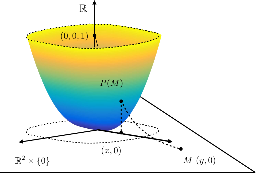
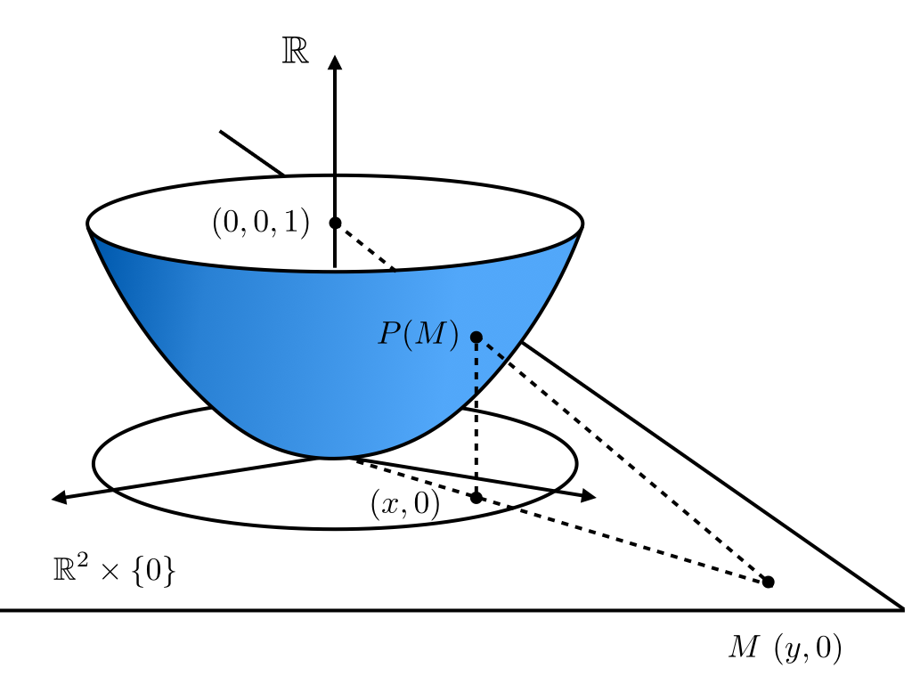
The name quasi-“parabolic” of Tparasubscript𝑇𝑝𝑎𝑟𝑎T_{para} comes from the homogeneous parabolic-type compactification; namely, Tparasubscript𝑇𝑝𝑎𝑟𝑎T_{para} with (α1,,αn)=(1,,1)subscript𝛼1subscript𝛼𝑛11(\alpha_{1},\cdots,\alpha_{n})=(1,\cdots,1) and c=1𝑐1c=1. In the homogeneous case, Tparasubscript𝑇𝑝𝑎𝑟𝑎T_{para} is the composite of the mapping from nsuperscript𝑛\mathbb{R}^{n} to a parabolic hypersurface {x12++xn2=xn+1}n+1superscriptsubscript𝑥12superscriptsubscript𝑥𝑛2subscript𝑥𝑛1superscript𝑛1\{x_{1}^{2}+\cdots+x_{n}^{2}=x_{n+1}\}\subset\mathbb{R}^{n+1} and the projection (x1,,xn,xn+1)(x1,,xn)maps-tosubscript𝑥1subscript𝑥𝑛subscript𝑥𝑛1subscript𝑥1subscript𝑥𝑛(x_{1},\cdots,x_{n},x_{n+1})\mapsto(x_{1},\cdots,x_{n}). In the homogeneous case α=(1,,1)𝛼11\alpha=(1,\cdots,1) and c=1𝑐1c=1, κ=κ(y)𝜅𝜅𝑦\kappa=\kappa(y) is explicitly given as κ(y)=12(1+1+4i=1nyi2)𝜅𝑦12114superscriptsubscript𝑖1𝑛superscriptsubscript𝑦𝑖2\kappa(y)=\frac{1}{2}\left(1+\sqrt{1+4\sum_{i=1}^{n}y_{i}^{2}}\right), which is also calculated from Fy(κ)=0subscript𝐹𝑦𝜅0F_{y}(\kappa)=0. See [4, 14] for details. Illustrations of parabolic and quasi-parabolic compactifications in two-dimensional situations are shown in Figure 1.

The quasi-parabolic compactification is an nontrivial example of admissible quasi-homogeneous compactifications. The biggest difference from quasi-Poincaré compactification is that the functional κ~α(x)subscript~𝜅𝛼𝑥\tilde{\kappa}_{\alpha}(x) does not contain any radicals. This property unconditionally guarantees the C1superscript𝐶1C^{1} smoothness of the desingularized vector field of good f𝑓f on 𝒟¯¯𝒟\overline{\mathcal{D}}. In particular, the stability analysis at infinity is available. Details are discussed in Section 3.
Refer to caption

(a)

Refer to caption

(b)

Figure 1: Parabolic and quasi-parabolic compactifications with type (2,1)21(2,1) for 2superscript2\mathbb{R}^{2}

Surfaces drawn here are (a) : ={(y1,y2,ζ)y12+y22=ζ}conditional-setsubscript𝑦1subscript𝑦2𝜁superscriptsubscript𝑦12superscriptsubscript𝑦22𝜁\mathcal{H}=\{(y_{1},y_{2},\zeta)\mid y_{1}^{2}+y_{2}^{2}=\zeta\} (parabolic compactification), and (b) : α={(y1,y2,ζ)y12+y24=ζ}subscript𝛼conditional-setsubscript𝑦1subscript𝑦2𝜁superscriptsubscript𝑦12superscriptsubscript𝑦24𝜁\mathcal{H}_{\alpha}=\{(y_{1},y_{2},\zeta)\mid y_{1}^{2}+y_{2}^{4}=\zeta\} (quasi-parabolic compactification with type (2,1)21(2,1)).

In both figures, the original phase space corresponds to 2×{0}2+1superscript20superscript21\mathbb{R}^{2}\times\{0\}\subset\mathbb{R}^{2+1} in the extended space. In the case of (a), the type α𝛼\alpha is chosen to be (1,1)11(1,1). The point P(M)𝑃𝑀P(M) show the intersection point between (0,0,1)001(0,0,1) and the given point M2𝑀superscript2M\in\mathbb{R}^{2} on \mathcal{H} and αsubscript𝛼\mathcal{H}_{\alpha} respectively, through the curve Cα(y)={((1ζ)α1y1,(1ζ)α2y2,ζ)}subscript𝐶𝛼𝑦superscript1𝜁subscript𝛼1subscript𝑦1superscript1𝜁subscript𝛼2subscript𝑦2𝜁C_{\alpha}(y)=\{((1-\zeta)^{\alpha_{1}}y_{1},(1-\zeta)^{\alpha_{2}}y_{2},\zeta)\}. Note that the curve Cαsubscript𝐶𝛼C_{\alpha} is just a straight line in the case of homogeneous compactification α=(1,1)𝛼11\alpha=(1,1). The projections of P(M)𝑃𝑀P(M) onto the original phase space; (x,0)𝑥0(x,0), are the images of (quasi-)parabolic compactifications, respectively. These observations can be easily generalized to nsuperscript𝑛\mathbb{R}^{n}.

2.4 Directional compactifications

There are several other compactifications reflecting (asymptotic) quasi-homogeneity of vector fields at infinity. For example, the transform y=(y1,,yn)(s,x)(s,x1,,xi1,xi+1,,xn)𝑦subscript𝑦1subscript𝑦𝑛maps-to𝑠𝑥𝑠subscript𝑥1subscript𝑥𝑖1subscript𝑥𝑖1subscript𝑥𝑛y=(y_{1},\cdots,y_{n})\mapsto(s,x)\equiv(s,x_{1},\cdots,x_{i-1},x_{i+1},\cdots,x_{n}) given by

yj=xjsαj(ji),yi=±1sαiformulae-sequencesubscript𝑦𝑗subscript𝑥𝑗superscript𝑠subscript𝛼𝑗𝑗𝑖subscript𝑦𝑖plus-or-minus1superscript𝑠subscript𝛼𝑖y_{j}=\frac{x_{j}}{s^{\alpha_{j}}}\quad(j\not=i),\quad y_{i}=\pm\frac{1}{s^{\alpha_{i}}} (2.4)

is a kind of compactifications, which corresponds the infinity to the subspace {s=0}𝑠0\{s=0\}\equiv\mathcal{E}. We shall call such a compactification a directional compactification with the type α=(α1,,αn)𝛼subscript𝛼1subscript𝛼𝑛\alpha=(\alpha_{1},\cdots,\alpha_{n}), according to [9]. The set ={s=0}𝑠0\mathcal{E}=\{s=0\} is called the horizon. This compactification is geometrically characterized as a local coordinate of quasi-Poincaré hemisphere of type α𝛼\alpha:

α:={(y1,,yn,s)n+11(1+p(y)2c)i=1nyi2βi+s2c=1},assignsubscript𝛼conditional-setsubscript𝑦1subscript𝑦𝑛𝑠superscript𝑛111𝑝superscript𝑦2𝑐superscriptsubscript𝑖1𝑛superscriptsubscript𝑦𝑖2subscript𝛽𝑖superscript𝑠2𝑐1\mathcal{H}_{\alpha}:=\left\{(y_{1},\cdots,y_{n},s)\in\mathbb{R}^{n+1}\mid\frac{1}{(1+p(y)^{2c})}\sum_{i=1}^{n}y_{i}^{2\beta_{i}}+s^{2c}=1\right\},

at (x1,,xn,s)=(0,,0,xi=±1,0,,0,0)(x_{1},\cdots,x_{n},s)=(0,\cdots,0,x_{i}=\pm 1,0,\cdots,0,0). See [9] for details. Note that, unlike admissible quasi-homogeneous compactifications in Definition 2.3, the coordinate representation (2.4) only makes sense in {±yi>0}plus-or-minussubscript𝑦𝑖0\{\pm y_{i}>0\}, in which sense directional compactifications are local ones. In particular, whenever we consider trajectories whose yisubscript𝑦𝑖y_{i}-component can change the sign, we have to take care of transformations among coordinate neighborhoods, which is quite tough for numerical integration of differential equations. Nevertheless, this compactification is still a very powerful tool if we consider solutions near infinity whose yisubscript𝑦𝑖y_{i}-component is known a priori to have identical sign.

3 Compactifications and dynamics at infinity

In this section, we calculate the vector field (2.1) under the admissible quasi-homogeneous compactification T𝑇T. Regard κ𝜅\kappa in the definition of T𝑇T as a function of y𝑦y. Integers {βi}i=1nsuperscriptsubscriptsubscript𝛽𝑖𝑖1𝑛\{\beta_{i}\}_{i=1}^{n} and c𝑐c in the definition of T𝑇T are assumed to satisfy (2.2). Differentiating x=T(y)𝑥𝑇𝑦x=T(y) with respect to t𝑡t, we have

xisuperscriptsubscript𝑥𝑖\displaystyle x_{i}^{\prime} =(yiκαi)=yiκαiαiyiκαi1κ2αiκabsentsuperscriptsubscript𝑦𝑖superscript𝜅subscript𝛼𝑖superscriptsubscript𝑦𝑖superscript𝜅subscript𝛼𝑖subscript𝛼𝑖subscript𝑦𝑖superscript𝜅subscript𝛼𝑖1superscript𝜅2subscript𝛼𝑖superscript𝜅\displaystyle=\left(\frac{y_{i}}{\kappa^{\alpha_{i}}}\right)^{\prime}=\frac{y_{i}^{\prime}}{\kappa^{\alpha_{i}}}-\frac{\alpha_{i}y_{i}\kappa^{\alpha_{i}-1}}{\kappa^{2\alpha_{i}}}\kappa^{\prime}
=yiκαiαiyiκαi+1κ,yabsentsuperscriptsubscript𝑦𝑖superscript𝜅subscript𝛼𝑖subscript𝛼𝑖subscript𝑦𝑖superscript𝜅subscript𝛼𝑖1𝜅superscript𝑦\displaystyle=\frac{y_{i}^{\prime}}{\kappa^{\alpha_{i}}}-\frac{\alpha_{i}y_{i}}{\kappa^{\alpha_{i}+1}}\langle\nabla\kappa,y^{\prime}\rangle
=fi(y)καiαiyiκαi+1κ,f(y).absentsubscript𝑓𝑖𝑦superscript𝜅subscript𝛼𝑖subscript𝛼𝑖subscript𝑦𝑖superscript𝜅subscript𝛼𝑖1𝜅𝑓𝑦\displaystyle=\frac{f_{i}(y)}{\kappa^{\alpha_{i}}}-\frac{\alpha_{i}y_{i}}{\kappa^{\alpha_{i}+1}}\langle\nabla\kappa,f(y)\rangle.

Namely,

x=Aα(fi(y)κ1f,κyα)superscript𝑥subscript𝐴𝛼subscript𝑓𝑖𝑦superscript𝜅1𝑓𝜅subscript𝑦𝛼x^{\prime}=A_{\alpha}\left(f_{i}(y)-\kappa^{-1}\langle f,\nabla\kappa\rangle y_{\alpha}\right) (3.1)

We have the one-to-one correspondence of bounded equilibria, which helps us with detecting dynamics at infinity.

Proposition 3.1.

The quasi-homogeneous compactification T𝑇T maps bounded equilibria of (2.1) in nsuperscript𝑛\mathbb{R}^{n} into equilibria of (3.1) in 𝒟𝒟\mathcal{D}, and vice versa.

Proof.

Suppose that ysubscript𝑦y_{\ast} is an equilibrium of (2.1), i.e., f(y)=0𝑓subscript𝑦0f(y_{\ast})=0. Then the right-hand side of (3.1) obviously vanishes at the corresponding xsubscript𝑥x_{\ast}.

Conversely, suppose that the right-hand side of (3.1) vanishes at a point x𝒟,p(x)<1formulae-sequence𝑥𝒟𝑝𝑥1x\in\mathcal{D},p(x)<1: namely,

f(κx)κ(y)1κ,f(κx)yα=0.𝑓𝜅𝑥𝜅superscript𝑦1𝜅𝑓𝜅𝑥subscript𝑦𝛼0f(\kappa x)-\kappa(y)^{-1}\langle\nabla\kappa,f(\kappa x)\rangle y_{\alpha}=0.

Multiplying κ𝜅\nabla\kappa, we have

κ,f(κx)(1κ(y)1κ,yα)=0.𝜅𝑓𝜅𝑥1𝜅superscript𝑦1𝜅subscript𝑦𝛼0\langle\nabla\kappa,f(\kappa x)\rangle\left(1-\kappa(y)^{-1}\langle\nabla\kappa,y_{\alpha}\rangle\right)=0.

Due to (A3), we have |κ(y)1κ,yα|<1𝜅superscript𝑦1𝜅subscript𝑦𝛼1|\kappa(y)^{-1}\langle\nabla\kappa,y_{\alpha}\rangle|<1 and hence κ,f(κx)=0𝜅𝑓𝜅𝑥0\langle\nabla\kappa,f(\kappa x)\rangle=0. Thus we have f(y)=f(κx)=0𝑓𝑦𝑓𝜅𝑥0f(y)=f(\kappa x)=0 by the assumption. ∎

Next we discuss the dynamics at infinity. Denoting

f~j(x1,,xn):=κ(k+αj)fj(κα1x1,,καnxn),j=1,,n,formulae-sequenceassignsubscript~𝑓𝑗subscript𝑥1subscript𝑥𝑛superscript𝜅𝑘subscript𝛼𝑗subscript𝑓𝑗superscript𝜅subscript𝛼1subscript𝑥1superscript𝜅subscript𝛼𝑛subscript𝑥𝑛𝑗1𝑛\tilde{f}_{j}(x_{1},\cdots,x_{n}):=\kappa^{-(k+\alpha_{j})}f_{j}(\kappa^{\alpha_{1}}x_{1},\cdots,\kappa^{\alpha_{n}}x_{n}),\quad j=1,\cdots,n, (3.2)

we have

xisuperscriptsubscript𝑥𝑖\displaystyle x_{i}^{\prime} =κk+αif~i(x)καiαiκαixiκαi+1j=1n(κ)jκk+αjf~j(x)absentsuperscript𝜅𝑘subscript𝛼𝑖subscript~𝑓𝑖𝑥superscript𝜅subscript𝛼𝑖subscript𝛼𝑖superscript𝜅subscript𝛼𝑖subscript𝑥𝑖superscript𝜅subscript𝛼𝑖1superscriptsubscript𝑗1𝑛subscript𝜅𝑗superscript𝜅𝑘subscript𝛼𝑗subscript~𝑓𝑗𝑥\displaystyle=\frac{\kappa^{k+\alpha_{i}}\tilde{f}_{i}(x)}{\kappa^{\alpha_{i}}}-\frac{\alpha_{i}\kappa^{\alpha_{i}}x_{i}}{\kappa^{\alpha_{i}+1}}\sum_{j=1}^{n}(\nabla\kappa)_{j}\kappa^{k+\alpha_{j}}\tilde{f}_{j}(x)
=κkf~i(x)αixij=1n(κ)jκk+αj1f~j(x).absentsuperscript𝜅𝑘subscript~𝑓𝑖𝑥subscript𝛼𝑖subscript𝑥𝑖superscriptsubscript𝑗1𝑛subscript𝜅𝑗superscript𝜅𝑘subscript𝛼𝑗1subscript~𝑓𝑗𝑥\displaystyle=\kappa^{k}\tilde{f}_{i}(x)-\alpha_{i}x_{i}\sum_{j=1}^{n}(\nabla\kappa)_{j}\kappa^{k+\alpha_{j}-1}\tilde{f}_{j}(x). (3.3)

Since κ𝜅\kappa\to\infty as p(x)1𝑝𝑥1p(x)\to 1, then the vector field has singularities at infinity, while f~j(x)subscript~𝑓𝑗𝑥\tilde{f}_{j}(x) themselves are continuous on 𝒟¯¯𝒟\overline{\mathcal{D}} because of the asymptotic quasi-homogeneity of f𝑓f. Nevertheless, admissibility of compactifications yields the following observation.

Lemma 3.2.

The right-hand side of (3) is O(κk)𝑂superscript𝜅𝑘O(\kappa^{k}) as κ𝜅\kappa\to\infty. In other words, the order with respect to κ𝜅\kappa is independent of i𝑖i.

Proof.

By admissibility (A1)-(A2), we have

(κ(y))i1αiyi2βi1κ(y)2c1=1αiκαi(2βi1)xi2βi1κ2c1=1αixi2βi1καi1 as p(y),formulae-sequencesimilar-tosubscript𝜅𝑦𝑖1subscript𝛼𝑖superscriptsubscript𝑦𝑖2subscript𝛽𝑖1𝜅superscript𝑦2𝑐11subscript𝛼𝑖superscript𝜅subscript𝛼𝑖2subscript𝛽𝑖1superscriptsubscript𝑥𝑖2subscript𝛽𝑖1superscript𝜅2𝑐11subscript𝛼𝑖superscriptsubscript𝑥𝑖2subscript𝛽𝑖1superscript𝜅subscript𝛼𝑖1 as 𝑝𝑦(\nabla\kappa(y))_{i}\sim\frac{1}{\alpha_{i}}\frac{y_{i}^{2\beta_{i}-1}}{\kappa(y)^{2c-1}}=\frac{1}{\alpha_{i}}\frac{\kappa^{\alpha_{i}(2\beta_{i}-1)}x_{i}^{2\beta_{i}-1}}{\kappa^{2c-1}}=\frac{1}{\alpha_{i}}\frac{x_{i}^{2\beta_{i}-1}}{\kappa^{\alpha_{i}-1}}\quad\text{ as }\quad p(y)\to\infty,

where we used the condition αjβjcsubscript𝛼𝑗subscript𝛽𝑗𝑐\alpha_{j}\beta_{j}\equiv c for all j𝑗j from (2.2). Therefore the vector field (3) near infinity becomes

xisuperscriptsubscript𝑥𝑖\displaystyle x_{i}^{\prime} κkf~i(x)αixij=1n1αjxj2βj1καj1κk+αj1f~j(x)similar-toabsentsuperscript𝜅𝑘subscript~𝑓𝑖𝑥subscript𝛼𝑖subscript𝑥𝑖superscriptsubscript𝑗1𝑛1subscript𝛼𝑗superscriptsubscript𝑥𝑗2subscript𝛽𝑗1superscript𝜅subscript𝛼𝑗1superscript𝜅𝑘subscript𝛼𝑗1subscript~𝑓𝑗𝑥\displaystyle\sim\kappa^{k}\tilde{f}_{i}(x)-\alpha_{i}x_{i}\sum_{j=1}^{n}\frac{1}{\alpha_{j}}\frac{x_{j}^{2\beta_{j}-1}}{\kappa^{\alpha_{j}-1}}\kappa^{k+\alpha_{j}-1}\tilde{f}_{j}(x)
=κk{f~i(x)αixij=1nxj2βj1αjf~j(x)} as κ.formulae-sequenceabsentsuperscript𝜅𝑘subscript~𝑓𝑖𝑥subscript𝛼𝑖subscript𝑥𝑖superscriptsubscript𝑗1𝑛superscriptsubscript𝑥𝑗2subscript𝛽𝑗1subscript𝛼𝑗subscript~𝑓𝑗𝑥 as 𝜅\displaystyle=\kappa^{k}\left\{\tilde{f}_{i}(x)-\alpha_{i}x_{i}\sum_{j=1}^{n}\frac{x_{j}^{2\beta_{j}-1}}{\alpha_{j}}\tilde{f}_{j}(x)\right\}\quad\text{ as }\quad\kappa\to\infty. (3.4)

Since f~isubscript~𝑓𝑖\tilde{f}_{i} is O(1)𝑂1O(1) as κ𝜅\kappa\to\infty, then right-hand side of (3.4) is O(κk)𝑂superscript𝜅𝑘O(\kappa^{k}) as κ𝜅\kappa\to\infty. ∎

Lemma 3.2 leads to introduce the following transformation of time variable.

Definition 3.3 (Time-variable desingularization).

Define the new time variable τ𝜏\tau depending on y𝑦y by

dτ=κ(y(t))kdt𝑑𝜏𝜅superscript𝑦𝑡𝑘𝑑𝑡d\tau=\kappa(y(t))^{k}dt (3.5)

namely,

tt0=τ0τdτκ(y(τ))k,𝑡subscript𝑡0superscriptsubscriptsubscript𝜏0𝜏𝑑𝜏𝜅superscript𝑦𝜏𝑘t-t_{0}=\int_{\tau_{0}}^{\tau}\frac{d\tau}{\kappa(y(\tau))^{k}},

where τ0subscript𝜏0\tau_{0} and t0subscript𝑡0t_{0} denote the correspondence of initial times, and y(τ)𝑦𝜏y(\tau) is the solution trajectory y(t)𝑦𝑡y(t) under the new time variable τ𝜏\tau. We shall call (3.5) the time-variable desingularization of (3) of order k+1𝑘1k+1.

x˙idxidτ=f~i(x)αixij=1n(κ)jκαj1f~j(x)gi(x).subscript˙𝑥𝑖𝑑subscript𝑥𝑖𝑑𝜏subscript~𝑓𝑖𝑥subscript𝛼𝑖subscript𝑥𝑖superscriptsubscript𝑗1𝑛subscript𝜅𝑗superscript𝜅subscript𝛼𝑗1subscript~𝑓𝑗𝑥subscript𝑔𝑖𝑥\dot{x}_{i}\equiv\frac{dx_{i}}{d\tau}=\tilde{f}_{i}(x)-\alpha_{i}x_{i}\sum_{j=1}^{n}(\nabla\kappa)_{j}\kappa^{\alpha_{j}-1}\tilde{f}_{j}(x)\equiv g_{i}(x). (3.6)

Summarizing the above observation, we have the extension of dynamics at infinity.

Proposition 3.4 (Extension of dynamics at infinity).

Let τ𝜏\tau be the new time variable given by (3.5). Then the dynamics (2.1) can be extended to the infinity in the sense that the vector field g𝑔g is continuous on 𝒟¯¯𝒟\overline{\mathcal{D}}.

Proof.

The component-wise desingularized vector field (3.6) is obviously continuous on 𝒟¯¯𝒟\overline{\mathcal{D}} since this consists of product and sum of continuous functions xisubscript𝑥𝑖x_{i}’s and f~isubscript~𝑓𝑖\tilde{f}_{i}’s on 𝒟¯¯𝒟\overline{\mathcal{D}}. ∎

Example 3.5 (Extension of vector fields via quasi-parabolic compactifications).

In the case of quasi-parabolic compactification, κ𝜅\nabla\kappa is given by

(yκ(y))j=2βjyj2βj12cκ2c1(12c12cκ1)=κ2cαjxj2βj1αjκ2c1(12c12cκ1)=xj2βj1αjκαj1(12c12cκ1).subscriptsubscript𝑦𝜅𝑦𝑗2subscript𝛽𝑗superscriptsubscript𝑦𝑗2subscript𝛽𝑗12𝑐superscript𝜅2𝑐112𝑐12𝑐superscript𝜅1superscript𝜅2𝑐subscript𝛼𝑗superscriptsubscript𝑥𝑗2subscript𝛽𝑗1subscript𝛼𝑗superscript𝜅2𝑐112𝑐12𝑐superscript𝜅1superscriptsubscript𝑥𝑗2subscript𝛽𝑗1subscript𝛼𝑗superscript𝜅subscript𝛼𝑗112𝑐12𝑐superscript𝜅1(\nabla_{y}\kappa(y))_{j}=\frac{2\beta_{j}y_{j}^{2\beta_{j}-1}}{2c\kappa^{2c-1}\left(1-\frac{2c-1}{2c}\kappa^{-1}\right)}=\frac{\kappa^{2c-\alpha_{j}}x_{j}^{2\beta_{j}-1}}{\alpha_{j}\kappa^{2c-1}\left(1-\frac{2c-1}{2c}\kappa^{-1}\right)}=\frac{x_{j}^{2\beta_{j}-1}}{\alpha_{j}\kappa^{\alpha_{j}-1}\left(1-\frac{2c-1}{2c}\kappa^{-1}\right)}.

We can see that g𝑔g in (3.6) can be extended to be C0superscript𝐶0C^{0} on 𝒟¯¯𝒟\overline{\mathcal{D}}.

Proposition 3.4 shows that the “dynamics and invariant sets at infinity” make sense. For example, “equilibria at infinity” defined below are well-defined.

Definition 3.6 (Equilibria at infinity).

We say that the vector field (2.1) has an equilibrium at infinity in the direction xsubscript𝑥x_{\ast} if xsubscript𝑥x_{\ast} is an equilibrium of (3.6) on 𝒟𝒟\partial{\mathcal{D}}.

Now divergent solutions are described in terms of trajectories asymptotic to equilibria on the horizon for desingularized vector fields.

Theorem 3.7 (Divergent solutions and asymptotic behavior).

Let y(t)𝑦𝑡y(t) be a solution of (2.1) with the interval of maximal existence time (a,b)𝑎𝑏(a,b), possibly a=𝑎a=-\infty and b=+𝑏b=+\infty. Assume that y𝑦y tends to infinity in the direction xsubscript𝑥x_{\ast} as tb0𝑡𝑏0t\to b-0 or ta+0𝑡𝑎0t\to a+0. Then xsubscript𝑥x_{\ast} is an equilibrium of (3.6) on \mathcal{E}.

Proof.

The property b=sup{ty(t) is a solution of (2.1)}𝑏supremumconditional-set𝑡𝑦𝑡 is a solution of (2.1)b=\sup\{t\mid y(t)\text{ is a solution of (\ref{ODE-original})}\} corresponds to the property that

sup{τx(τ)=T(y(t)) is a solution of (3.6) in the time variable τ}=.supremumconditional-set𝜏𝑥𝜏𝑇𝑦𝑡 is a solution of (3.6) in the time variable τ\sup\{\tau\mid x(\tau)=T(y(t))\text{ is a solution of (\ref{ODE-desing}) in the time variable $\tau$}\}=\infty.

Indeed, if not, then ττ0<𝜏subscript𝜏0\tau\to\tau_{0}<\infty and limττ00x(τ)=xsubscript𝜏subscript𝜏00𝑥𝜏subscript𝑥\lim_{\tau\to\tau_{0}-0}x(\tau)=x_{\ast} as tb0𝑡𝑏0t\to b-0. The condition x(τ)=x𝑥𝜏subscript𝑥x(\tau)=x_{\ast} is the regular initial condition of (3.6). The vector field (3.6) with the new initial point x(τ)=x𝑥𝜏subscript𝑥x(\tau)=x_{\ast} thus has a locally unique solution x(τ)𝑥𝜏x(\tau) in a neighborhood of τ0subscript𝜏0\tau_{0}, which contradicts the maximality of b𝑏b. Therefore we know that τ+𝜏\tau\to+\infty as tb0𝑡𝑏0t\to b-0. Since limτx(τ)=xsubscript𝜏𝑥𝜏subscript𝑥\lim_{\tau\to\infty}x(\tau)=x_{\ast}, then xsubscript𝑥x_{\ast} is an equilibrium of (3.6) on 𝒟𝒟\partial{\mathcal{D}}. The similar arguments show that ta+0𝑡𝑎0t\to a+0 corresponds to τ𝜏\tau\to-\infty and that the same consequence holds true. ∎

This theorem shows that divergent solutions in the direction xsubscript𝑥x_{\ast} correspond to trajectories of (3.6) on the stable manifold Ws(x)superscript𝑊𝑠subscript𝑥W^{s}(x_{\ast})333 The stable set Ws(p)superscript𝑊𝑠𝑝W^{s}(p) of a point p𝑝p is characterized as {x=x(0)d(x(τ),p)0 as τ}conditional-set𝑥𝑥0𝑑𝑥𝜏𝑝0 as 𝜏\{x=x(0)\mid d(x(\tau),p)\to 0\text{ as }\tau\to\infty\} with a metric d𝑑d on the phase space. If p𝑝p is an equilibrium, the (center-)stable manifold theorem indicates that the set Ws(p)superscript𝑊𝑠𝑝W^{s}(p) is, at least locally, has a smooth manifold structure, which is called a (local) stable manifold of p𝑝p. of the equilibrium xsubscript𝑥x_{\ast}. This correspondence opens the door to applications of various results in dynamical systems to divergent solutions. Before moving to the blow-up argument, we gather several properties of dynamics at infinity, which will be useful to concrete studies.

Theorem 3.8 (Dynamics at infinity, cf. [9]).
  1. 1.

    The horizon =𝒟𝒟\mathcal{E}=\partial{\mathcal{D}} is an invariant manifold of (3.6).

  2. 2.

    Dynamics of (3.6) on \mathcal{E} is dominated by

    x˙i=(f~α,k)i(j=1nβjx2βj1(f~α,k)j)xiβi.subscript˙𝑥𝑖subscriptsubscript~𝑓𝛼𝑘𝑖superscriptsubscript𝑗1𝑛subscript𝛽𝑗superscript𝑥2subscript𝛽𝑗1subscriptsubscript~𝑓𝛼𝑘𝑗subscript𝑥𝑖subscript𝛽𝑖\dot{x}_{i}=(\tilde{f}_{\alpha,k})_{i}-\left(\sum_{j=1}^{n}\beta_{j}x^{2\beta_{j}-1}(\tilde{f}_{\alpha,k})_{j}\right)\frac{x_{i}}{\beta_{i}}.
  3. 3.

    Time evolution of 1p(x)2c1𝑝superscript𝑥2𝑐1-p(x)^{2c} in τ𝜏\tau-time scale is dominated by

    ddτ(1p(x)2c)=(j=1nβjxj2βj1f~j)(1p(x)2c).𝑑𝑑𝜏1𝑝superscript𝑥2𝑐superscriptsubscript𝑗1𝑛subscript𝛽𝑗superscriptsubscript𝑥𝑗2subscript𝛽𝑗1subscript~𝑓𝑗1𝑝superscript𝑥2𝑐\frac{d}{d\tau}(1-p(x)^{2c})=-\left(\sum_{j=1}^{n}\beta_{j}x_{j}^{2\beta_{j}-1}\tilde{f}_{j}\right)(1-p(x)^{2c}).
  4. 4.

    Assume that the vector field f𝑓f in (2.1) is quasi-homogeneous of type (α1,,αn)subscript𝛼1subscript𝛼𝑛(\alpha_{1},\cdots,\alpha_{n}) and order k+1𝑘1k+1. Then the desingularized vector field g𝑔g given in (3.6) satisfies

    gi((1)α1x1,,(1)αnxn)=(1)k+αngi(x1,,xn).subscript𝑔𝑖superscript1subscript𝛼1subscript𝑥1superscript1subscript𝛼𝑛subscript𝑥𝑛superscript1𝑘subscript𝛼𝑛subscript𝑔𝑖subscript𝑥1subscript𝑥𝑛g_{i}((-1)^{\alpha_{1}}x_{1},\cdots,(-1)^{\alpha_{n}}x_{n})=(-1)^{k+\alpha_{n}}g_{i}(x_{1},\cdots,x_{n}). (3.7)

    In particular, for any asymptotically quasi-homogeneous vector field f𝑓f in (2.1) of type (α1,,αn)subscript𝛼1subscript𝛼𝑛(\alpha_{1},\cdots,\alpha_{n}) and order k+1𝑘1k+1, the desingularized vector field g𝑔g satisfies (3.7) on \mathcal{E}.

Proof.

See [9]. ∎

Remark 3.9.

Theorem 3.8-4 shows that the vector field at infinity is equivariant with respect to the symmetry ια(x)subscript𝜄𝛼𝑥\iota_{\alpha}(x) defined as

(x1,,xn)ια(x)((1)α1x1,,(1)αnxn).maps-tosubscript𝑥1subscript𝑥𝑛subscript𝜄𝛼𝑥superscript1subscript𝛼1subscript𝑥1superscript1subscript𝛼𝑛subscript𝑥𝑛(x_{1},\cdots,x_{n})\mapsto\iota_{\alpha}(x)\equiv((-1)^{\alpha_{1}}x_{1},\cdots,(-1)^{\alpha_{n}}x_{n}).

on \mathcal{E}. In particular, if x𝑥x\in\mathcal{E} is an equilibrium of (3.6), then so is ια(x)subscript𝜄𝛼𝑥\iota_{\alpha}(x). In the homogeneous case, the symmetry is just ια(x)=xsubscript𝜄𝛼𝑥𝑥\iota_{\alpha}(x)=-x, as stated in Proposition 2.6 of [4].

3.1 Desingularized vector field with quasi-parabolic compactifications

In the case of quasi-parabolic compactifications, there is an alternative time-variable desingularization given as follows.

Definition 3.10 (Time-variable desingularization for quasi-parabolic compactifications).

Let y(t)𝑦𝑡y(t) be a solution of (2.1) with an asymptotically quasi-homogeneous vector field f𝑓f of type α𝛼\alpha and order k+1𝑘1k+1. Let also x=Tpara(y)𝑥subscript𝑇𝑝𝑎𝑟𝑎𝑦x=T_{para}(y) be the image of y𝑦y via the quasi-parabolic compactification of type α𝛼\alpha. Define the new time variable τ𝜏\tau depending on y(t)𝑦𝑡y(t) by

dτ=κ(y(t))k(12c12cκ1)1dt=(1p(x)2c)k(12c12c(1p(x)2c))1dt.𝑑𝜏𝜅superscript𝑦𝑡𝑘superscript12𝑐12𝑐superscript𝜅11𝑑𝑡superscript1𝑝superscript𝑥2𝑐𝑘superscript12𝑐12𝑐1𝑝superscript𝑥2𝑐1𝑑𝑡d\tau=\kappa(y(t))^{k}\left(1-\frac{2c-1}{2c}\kappa^{-1}\right)^{-1}dt=(1-p(x)^{2c})^{-k}\left(1-\frac{2c-1}{2c}(1-p(x)^{2c})\right)^{-1}dt. (3.8)

We shall call (3.8) the quasi-parabolic time-variable desingularization of (3).

In the case of quasi-Poincaré compactifications, the desingularized vector field g𝑔g associated with the vector field f𝑓f is not always C1superscript𝐶1C^{1} even if f𝑓f is sufficiently smooth because of the presence of radicals in κ𝜅\kappa (see [9]). On the other hand, in the case of quasi-parabolic compactifications, if f𝑓f is smooth, the corresponding desingularized vector field can be always smooth on 𝒟¯¯𝒟\overline{\mathcal{D}} with the alternative time-variable desingularization. This big difference is one of the reasons why we introduce an alternative quasi-homogeneous compactifications, which is mentioned again in Section 4.

Proposition 3.11.

Let f𝑓f be an asymptotically quasi-homogeneous, C1superscript𝐶1C^{1} vector field f𝑓f of type α𝛼\alpha and order k+1𝑘1k+1. Let x=Tpara(y)𝑥subscript𝑇𝑝𝑎𝑟𝑎𝑦x=T_{para}(y) be a new variable through quasi-parabolic compactification. Then the vector field associated with (3) and τ𝜏\tau-timescale given in (3.8) is C1superscript𝐶1C^{1} on 𝒟¯¯𝒟\overline{\mathcal{D}}.

Proof.

The desingularized vector field in the time variable τ𝜏\tau given in (3.8) is

dxidτ=(12c12c(1p(x)2c))f~i(x)αixij=1nxj2βj1αjf~j(x).𝑑subscript𝑥𝑖𝑑𝜏12𝑐12𝑐1𝑝superscript𝑥2𝑐subscript~𝑓𝑖𝑥subscript𝛼𝑖subscript𝑥𝑖superscriptsubscript𝑗1𝑛superscriptsubscript𝑥𝑗2subscript𝛽𝑗1subscript𝛼𝑗subscript~𝑓𝑗𝑥\frac{dx_{i}}{d\tau}=\left(1-\frac{2c-1}{2c}(1-p(x)^{2c})\right)\tilde{f}_{i}(x)-\alpha_{i}x_{i}\sum_{j=1}^{n}\frac{x_{j}^{2\beta_{j}-1}}{\alpha_{j}}\tilde{f}_{j}(x). (3.9)

Note that each f~j(x)subscript~𝑓𝑗𝑥\tilde{f}_{j}(x) is C1superscript𝐶1C^{1} on 𝒟¯¯𝒟\overline{\mathcal{D}}, since all terms of f~jsubscript~𝑓𝑗\tilde{f}_{j} are multiples of powers of (1p(x)2c)1𝑝superscript𝑥2𝑐(1-p(x)^{2c}) and smooth asymptotically quasi-homogeneous terms in fj(y)subscript𝑓𝑗𝑦f_{j}(y). Consequently, we know that the right-hand side of (3.9) is C1superscript𝐶1C^{1} on 𝒟¯¯𝒟\overline{\mathcal{D}}. ∎

3.2 Desingularized vector field with directional compactifications

The desingularized vector field associated with f𝑓f is also considered with directional compactifications like (2.4). For simplicity, set i=n𝑖𝑛i=n in (2.4). The corresponding dynamics in t𝑡t-timescale is then calculated as follows:

(y1y2yn)=(α1s(α1+1)x1sα100α2s(α2+1)x20sα20αn1s(αn1+1)00sαn1αns(αn+1)000)(sx1x2xn1)Ds(sx1x2xn1).matrixsuperscriptsubscript𝑦1superscriptsubscript𝑦2superscriptsubscript𝑦𝑛matrixsubscript𝛼1superscript𝑠subscript𝛼11subscript𝑥1superscript𝑠subscript𝛼100subscript𝛼2superscript𝑠subscript𝛼21subscript𝑥20superscript𝑠subscript𝛼20subscript𝛼𝑛1superscript𝑠subscript𝛼𝑛1100superscript𝑠subscript𝛼𝑛1subscript𝛼𝑛superscript𝑠subscript𝛼𝑛1000matrixsuperscript𝑠superscriptsubscript𝑥1superscriptsubscript𝑥2superscriptsubscript𝑥𝑛1subscript𝐷𝑠matrixsuperscript𝑠superscriptsubscript𝑥1superscriptsubscript𝑥2superscriptsubscript𝑥𝑛1\begin{pmatrix}y_{1}^{\prime}\\ y_{2}^{\prime}\\ \vdots\\ y_{n}^{\prime}\end{pmatrix}=\begin{pmatrix}-\alpha_{1}s^{-(\alpha_{1}+1)}x_{1}&s^{-\alpha_{1}}&0&\cdots&0\\ -\alpha_{2}s^{-(\alpha_{2}+1)}x_{2}&0&s^{-\alpha_{2}}&\cdots&0\\ \vdots&\vdots&\vdots&\ddots&\vdots\\ -\alpha_{n-1}s^{-(\alpha_{n-1}+1)}&0&0&\cdots&s^{-\alpha_{n-1}}\\ -\alpha_{n}s^{-(\alpha_{n}+1)}&0&0&\cdots&0\end{pmatrix}\begin{pmatrix}s^{\prime}\\ x_{1}^{\prime}\\ x_{2}^{\prime}\\ \vdots\\ x_{n-1}^{\prime}\end{pmatrix}\equiv D_{s}\begin{pmatrix}s^{\prime}\\ x_{1}^{\prime}\\ x_{2}^{\prime}\\ \vdots\\ x_{n-1}^{\prime}\end{pmatrix}. (3.10)

It follows that the matrix Dssubscript𝐷𝑠D_{s} is written by the following product of matrices (see also [9]):

Ds=(sα1000sα2000sαn)(α1x1100α2x2010αn1xn1001αn000)(s100010001).subscript𝐷𝑠matrixsuperscript𝑠subscript𝛼1000superscript𝑠subscript𝛼2000superscript𝑠subscript𝛼𝑛matrixsubscript𝛼1subscript𝑥1100subscript𝛼2subscript𝑥2010subscript𝛼𝑛1subscript𝑥𝑛1001subscript𝛼𝑛000matrixsuperscript𝑠100010001D_{s}=\begin{pmatrix}s^{-\alpha_{1}}&0&\cdots&0\\ 0&s^{-\alpha_{2}}&\cdots&0\\ \vdots&\vdots&\ddots&\vdots\\ 0&0&\cdots&s^{-\alpha_{n}}\end{pmatrix}\begin{pmatrix}\alpha_{1}x_{1}&1&0&\cdots&0\\ \alpha_{2}x_{2}&0&1&\cdots&0\\ \vdots&\vdots&\vdots&\ddots&\vdots\\ \alpha_{n-1}x_{n-1}&0&0&\cdots&1\\ \alpha_{n}&0&0&\cdots&0\end{pmatrix}\begin{pmatrix}-s^{-1}&0&\cdots&0\\ 0&1&\cdots&0\\ \vdots&\vdots&\ddots&\vdots\\ 0&0&\cdots&1\end{pmatrix}.

Since αi>0subscript𝛼𝑖0\alpha_{i}>0 for all i𝑖i, then the matrix Dssubscript𝐷𝑠D_{s} is invertible on {s>0}×n𝑠0superscript𝑛\{s>0\}\times\mathbb{R}^{n} to obtain

Ds1=(s00010001)B(sα1000sα2000sαn),superscriptsubscript𝐷𝑠1matrix𝑠00010001𝐵matrixsuperscript𝑠subscript𝛼1000superscript𝑠subscript𝛼2000superscript𝑠subscript𝛼𝑛D_{s}^{-1}=\begin{pmatrix}-s&0&\cdots&0\\ 0&1&\cdots&0\\ \vdots&\vdots&\ddots&\vdots\\ 0&0&\cdots&1\end{pmatrix}B\begin{pmatrix}s^{\alpha_{1}}&0&\cdots&0\\ 0&s^{\alpha_{2}}&\cdots&0\\ \vdots&\vdots&\ddots&\vdots\\ 0&0&\cdots&s^{\alpha_{n}}\end{pmatrix},

where B𝐵B is the inverse444 The existence of B𝐵B immediately follows by cyclic permutations and the fact that αn>0subscript𝛼𝑛0\alpha_{n}>0. of the matrix

(α1x1100α2x2010αn1xn1001αn000).matrixsubscript𝛼1subscript𝑥1100subscript𝛼2subscript𝑥2010subscript𝛼𝑛1subscript𝑥𝑛1001subscript𝛼𝑛000\begin{pmatrix}\alpha_{1}x_{1}&1&0&\cdots&0\\ \alpha_{2}x_{2}&0&1&\cdots&0\\ \vdots&\vdots&\vdots&\ddots&\vdots\\ \alpha_{n-1}x_{n-1}&0&0&\cdots&1\\ \alpha_{n}&0&0&\cdots&0\end{pmatrix}.

Therefore (3.10) in {s>0}×n1𝑠0superscript𝑛1\{s>0\}\times\mathbb{R}^{n-1} is equivalent to

(sx1xn1)=(s00010001)B(sα1000sα2000sαn)(y1y2yn).matrixsuperscript𝑠superscriptsubscript𝑥1superscriptsubscript𝑥𝑛1matrix𝑠00010001𝐵matrixsuperscript𝑠subscript𝛼1000superscript𝑠subscript𝛼2000superscript𝑠subscript𝛼𝑛matrixsuperscriptsubscript𝑦1superscriptsubscript𝑦2superscriptsubscript𝑦𝑛\begin{pmatrix}s^{\prime}\\ x_{1}^{\prime}\\ \vdots\\ x_{n-1}^{\prime}\end{pmatrix}=\begin{pmatrix}-s&0&\cdots&0\\ 0&1&\cdots&0\\ \vdots&\vdots&\ddots&\vdots\\ 0&0&\cdots&1\end{pmatrix}B\begin{pmatrix}s^{\alpha_{1}}&0&\cdots&0\\ 0&s^{\alpha_{2}}&\cdots&0\\ \vdots&\vdots&\ddots&\vdots\\ 0&0&\cdots&s^{\alpha_{n}}\end{pmatrix}\begin{pmatrix}y_{1}^{\prime}\\ y_{2}^{\prime}\\ \vdots\\ y_{n}^{\prime}\end{pmatrix}. (3.11)

Similarly to (3.2), let

f^j(s,x1,,xn1):=sk+αjfj(sα1x1,,sαn1xn1,sαn),j=1,,n.formulae-sequenceassignsubscript^𝑓𝑗𝑠subscript𝑥1subscript𝑥𝑛1superscript𝑠𝑘subscript𝛼𝑗subscript𝑓𝑗superscript𝑠subscript𝛼1subscript𝑥1superscript𝑠subscript𝛼𝑛1subscript𝑥𝑛1superscript𝑠subscript𝛼𝑛𝑗1𝑛\hat{f}_{j}(s,x_{1},\cdots,x_{n-1}):=s^{k+\alpha_{j}}f_{j}(s^{-\alpha_{1}}x_{1},\cdots,s^{-\alpha_{n-1}}x_{n-1},s^{-\alpha_{n}}),\quad j=1,\cdots,n. (3.12)

Then (3.11) is rewritten as

(sx1xn1)=sk(s00010001)B(f^1f^2f^n).matrixsuperscript𝑠superscriptsubscript𝑥1superscriptsubscript𝑥𝑛1superscript𝑠𝑘matrix𝑠00010001𝐵matrixsubscript^𝑓1subscript^𝑓2subscript^𝑓𝑛\begin{pmatrix}s^{\prime}\\ x_{1}^{\prime}\\ \vdots\\ x_{n-1}^{\prime}\end{pmatrix}=s^{-k}\begin{pmatrix}-s&0&\cdots&0\\ 0&1&\cdots&0\\ \vdots&\vdots&\ddots&\vdots\\ 0&0&\cdots&1\end{pmatrix}B\begin{pmatrix}\hat{f}_{1}\\ \hat{f}_{2}\\ \vdots\\ \hat{f}_{n}\end{pmatrix}. (3.13)

The form of f^isubscript^𝑓𝑖\hat{f}_{i} in (3.12) and asymptotic quasi-homogeneity of fisubscript𝑓𝑖f_{i} and s𝑠s-independence of the matrix B𝐵B immediately yield the following consequence, which is the directional compactifications’ analogue of Lemma 3.2.

Lemma 3.12.

The right-hand side of (3.13) is O(sk)𝑂superscript𝑠𝑘O(s^{-k}) as s0𝑠0s\to 0. More precisely, the s𝑠s-component of (3.13) is O(sk+1)𝑂superscript𝑠𝑘1O(s^{-k+1}) as s0𝑠0s\to 0.

Lemma 3.12 leads to introduce the following transformation of time variable.

Definition 3.13 (Time-variable desingularization: directional compactification version).

Define the new time variable τdsubscript𝜏𝑑\tau_{d} by

dτd=s(t)kdt𝑑subscript𝜏𝑑𝑠superscript𝑡𝑘𝑑𝑡d\tau_{d}=s(t)^{-k}dt (3.14)

equivalently,

tt0=τ0τs(τd)k𝑑τd,𝑡subscript𝑡0superscriptsubscriptsubscript𝜏0𝜏𝑠superscriptsubscript𝜏𝑑𝑘differential-dsubscript𝜏𝑑t-t_{0}=\int_{\tau_{0}}^{\tau}s(\tau_{d})^{k}d\tau_{d},

where τ0subscript𝜏0\tau_{0} and t0subscript𝑡0t_{0} denote the correspondence of initial times, and s(τd)𝑠subscript𝜏𝑑s(\tau_{d}) is the solution trajectory s(t)𝑠𝑡s(t) under the parameter τ𝜏\tau. We shall call (3.14) the time-variable desingularization of (3.13) of order k+1𝑘1k+1.

The vector field (3.13) is then desingularized in τdsubscript𝜏𝑑\tau_{d}-time scale:

(dsdτddx1dτddxn1dτd)=(s00010001)B(f^1f^2f^n)gd(s,x1,,xn1).matrix𝑑𝑠𝑑subscript𝜏𝑑𝑑subscript𝑥1𝑑subscript𝜏𝑑𝑑subscript𝑥𝑛1𝑑subscript𝜏𝑑matrix𝑠00010001𝐵matrixsubscript^𝑓1subscript^𝑓2subscript^𝑓𝑛subscript𝑔𝑑𝑠subscript𝑥1subscript𝑥𝑛1\begin{pmatrix}\frac{ds}{d\tau_{d}}\\ \frac{dx_{1}}{d\tau_{d}}\\ \vdots\\ \frac{dx_{n-1}}{d\tau_{d}}\end{pmatrix}=\begin{pmatrix}-s&0&\cdots&0\\ 0&1&\cdots&0\\ \vdots&\vdots&\ddots&\vdots\\ 0&0&\cdots&1\end{pmatrix}B\begin{pmatrix}\hat{f}_{1}\\ \hat{f}_{2}\\ \vdots\\ \hat{f}_{n}\end{pmatrix}\equiv g_{d}(s,x_{1},\cdots,x_{n-1}). (3.15)

In particular, we have the following proposition.

Proposition 3.14.

Let τdsubscript𝜏𝑑\tau_{d} be the new time variable given by (3.14). Then the vector field gdsubscript𝑔𝑑g_{d} in (3.15) is continuous on {s0}×n1𝑠0superscript𝑛1\{s\geq 0\}\times\mathbb{R}^{n-1}.

Equilibria at infinity under directional compactifications are then characterized as equilibria for (3.15) on the horizon ={s=0}𝑠0\mathcal{E}=\{s=0\}. Note that gdsubscript𝑔𝑑g_{d} is smooth on {s0}×n1𝑠0superscript𝑛1\{s\geq 0\}\times\mathbb{R}^{n-1} if f𝑓f is smooth. In [9], the topological equivalence among desingularized vector fields with quasi-Poincaré compactifications and with directional compactifications including the horizon is discussed. In other words, dynamics of desingularized vector fields around the horizon is topologically identical among these compactifications. An essence of such a result is the admissibility in the sense of Definition 2.3 for the equivalence, which indicates that the equivalence result is also valid for quasi-parabolic compactifications.

4 Blow-up criteria and numerical validation procedure

Theorem 3.7 indicates that divergent solutions are described as trajectories on stable manifolds of equilibria on the horizon \mathcal{E} for (3.6). On the other hand, Theorem 3.7 itself does not distinguish blow-up solutions from divergent solutions. Under additional assumptions to equilibria on \mathcal{E}, we can characterize blow-up solutions from the viewpoint of dynamical systems. In this section, we firstly review a criterion of blow-ups discussed in [9]. Then we provide a methodology for explicit estimates of maximal existence time tmaxsubscript𝑡t_{\max}. Finally, we give an algorithm for validating blow-up solutions with computer assistance.

4.1 Blow-up criterion

Firstly we review an abstract result of blow-up criterion via quasi-homogeneous compactifications. For a squared matrix A𝐴A, Spec(A)Spec𝐴{\rm Spec}(A) denotes the set of eigenvalues of A𝐴A.

Proposition 4.1 (Stationary blow-up, [9]).

Assume that (2.1) has an equilibrium at infinity in the direction xsubscript𝑥x_{\ast}. Suppose that the desingularized vector field g𝑔g in (3.6) is C1superscript𝐶1C^{1} on 𝒟¯¯𝒟\overline{\mathcal{D}}, and that xsubscript𝑥x_{\ast} is hyperbolic for (3.6); namely all elements in Spec(Dg(x))Spec𝐷𝑔subscript𝑥{\rm Spec}(Dg(x_{\ast})) are away from the imaginary axis. Then the solution y(t)𝑦𝑡y(t) of (2.1) whose image x=T(y)𝑥𝑇𝑦x=T(y) is on Ws(x)superscript𝑊𝑠subscript𝑥W^{s}(x_{\ast}) in the desingularized vector field (3.6) satisfies tmax<subscript𝑡t_{\max}<\infty; namely, y(t)𝑦𝑡y(t) is a blow-up solution. Moreover,

p(y(t))c(tmaxt)1/k as ttmax,formulae-sequencesimilar-to𝑝𝑦𝑡𝑐superscriptsubscript𝑡𝑡1𝑘 as 𝑡subscript𝑡p(y(t))\sim c(t_{\max}-t)^{-1/k}\quad\text{ as }\quad t\to t_{\max},

where k+1𝑘1k+1 is the order of asymptotically quasi-homogeneous vector field f𝑓f. Finally, if the i𝑖i-th component (x)isubscriptsubscript𝑥𝑖(x_{\ast})_{i} of xsubscript𝑥x_{\ast} is not zero, then we also have

yi(t)c(tmaxt)αi/k as ttmax.formulae-sequencesimilar-tosubscript𝑦𝑖𝑡𝑐superscriptsubscript𝑡𝑡subscript𝛼𝑖𝑘 as 𝑡subscript𝑡y_{i}(t)\sim c(t_{\max}-t)^{-\alpha_{i}/k}\quad\text{ as }\quad t\to t_{\max}.

Proposition 4.1 gives us the slogan that hyperbolic equilibria at infinity induce blow-up solutions. In the above original version of blow-up criterion stated as above, the C1superscript𝐶1C^{1}-smoothness of the desingularized vector field g𝑔g in (3.6) is assumed, because such a smoothness is nontrivial for quasi-Poincaré compactifications even if f𝑓f is sufficiently smooth. On the other hand, Proposition 3.11 shows that stability analysis of equilibria at infinity always makes sense with quasi-parabolic compactifications, because in which case the desingularized vector field g𝑔g is always C1superscript𝐶1C^{1} on 𝒟¯¯𝒟\overline{\mathcal{D}} if f𝑓f is C1superscript𝐶1C^{1}.

Needless to say, the above proposition does not provide information of concrete blow-up time tmaxsubscript𝑡t_{\max} depending on initial data. In the successive subsections, we provide a validation procedure of blow-up solutions with explicit estimates of blow-up times.

4.2 Lyapunov functions around asymptotically stable equilibria

Our main tool for validating blow-up time is Lyapunov function, which describes the monotonous behavior of trajectories in terms of its value. As the general setting, consider the vector field

dxdt=f(x),f:nn: smooth.:𝑑𝑥𝑑𝑡𝑓𝑥𝑓superscript𝑛superscript𝑛: smooth\frac{dx}{dt}=f(x),\quad f:\mathbb{R}^{n}\to\mathbb{R}^{n}\text{: smooth}. (4.1)

For xn𝑥superscript𝑛x\in\mathbb{R}^{n}, Df(x)𝐷𝑓𝑥Df(x) denotes the Jacobian matrix of f𝑓f at x𝑥x.

Proposition 4.2 (Lyapunov function for stable equilibria, [10]).

Let xsubscript𝑥x_{\ast} be an equilibrium for (4.1) in a compact star-shaped set Nn𝑁superscript𝑛N\subset\mathbb{R}^{n}. Assume that there is a real symmetric matrix Y𝑌Y such that the matrix

A(x):=Df(x)TY+YDf(x)assign𝐴𝑥𝐷𝑓superscript𝑥𝑇𝑌𝑌𝐷𝑓𝑥A(x):=Df(x)^{T}Y+YDf(x) (4.2)

is strictly negative definite for all xN𝑥𝑁x\in N. Then the functional L:n:𝐿superscript𝑛L:\mathbb{R}^{n}\to\mathbb{R} given by

L(x):=(xx)TY(xx)assign𝐿𝑥superscript𝑥subscript𝑥𝑇𝑌𝑥subscript𝑥L(x):=(x-x_{\ast})^{T}Y(x-x_{\ast}) (4.3)

is a Lyapunov function on N𝑁N such that dL/dt𝑑𝐿𝑑𝑡dL/dt vanishes at xsubscript𝑥x_{\ast}. In particular, xsubscript𝑥x_{\ast} is the unique equilibrium in N𝑁N. If further the matrix Y𝑌Y is chosen to be positive definite, then the equilibrium xsubscript𝑥x_{\ast} is asymptotically stable.

We shall call the compact set N𝑁N satisfying the assumption in Proposition 4.2 a Lyapunov domain of xsubscript𝑥x_{\ast}.

Remark 4.3 (The present choice of L(x)𝐿𝑥L(x)).

Roughly speaking, the matrix Y𝑌Y contains information of sign of the real part of each Spec(Df(x))Spec𝐷𝑓𝑥{\rm Spec}(Df(x)) and a matrix representing change of coordinates. In the present case, we only treat asymptotically stable equilibria, which indicates that signs of ReλRe𝜆{\rm Re}\lambda for any λSpec(Df(x))𝜆Spec𝐷𝑓𝑥\lambda\in{\rm Spec}(Df(x)) should be identically negative. Before validating an equilibrium xsubscript𝑥x_{\ast}, it should be usually computed in a numerical (i.e., non-rigorous computation) sense with associated eigenvalues for finding candidates of validating equilibrium.

When we numerically compute eigenvalues of a Jacobian matrix, say Df(x)𝐷𝑓𝑥Df(x), we also compute eigenvectors to construct the eigenmatrix X𝑋X, which represents change of coordinates to an orthogonal one. In [10], the matrix Y𝑌Y in (4.3) is typically defined as Y=Re(XHX1)𝑌Resuperscript𝑋𝐻superscript𝑋1Y={\rm Re}(X^{-H}X^{-1}), where XH:=(X1)Hassignsuperscript𝑋𝐻superscriptsuperscript𝑋1𝐻X^{-H}:=(X^{-1})^{H} and Hsuperscript𝐻\ast^{H} denotes the Hermitian transpose of the object (vectors or matrices). Note that, in which case, the equilibrium xsubscript𝑥x_{\ast} is shown to be asymptotically stable in N𝑁N. However, there are cases that an eigenvalue has multiplicity larger than 111, in which cases the validation is failed because the computed eigenmatrix X𝑋X typically becomes singular. Indeed, our example below contains such a case.

One way to avoid such difficulty is to use the real Schur decomposition of the matrix Df(x)𝐷𝑓𝑥Df(x) instead of eigenpair computations. See Appendix A about a quick review of Schur decompositions of matrices. Let Q𝑄Q be a matrix such that QTDf(x)Qsuperscript𝑄𝑇𝐷𝑓𝑥𝑄Q^{T}Df(x)Q is a real upper triangle matrix for some point x𝑥x. Then we can check the sign of ReλRe𝜆{\rm Re}\lambda for all λSpec(Df(x))𝜆Spec𝐷𝑓𝑥\lambda\in{\rm Spec}(Df(x)). We then choose the matrix Q𝑄Q as a change of coordinates instead of the eigenmatrix X𝑋X. In such a case, the corresponding matrix Y𝑌Y is Y=Re(QHQ1)𝑌Resuperscript𝑄𝐻superscript𝑄1Y={\rm Re}(Q^{-H}Q^{-1}). When we use the real Schur decomposition, Q𝑄Q is an orthogonal real matrix. Then we take Y=I𝑌𝐼Y=I: the identity matrix, which shows that our Lyapunov function L𝐿L becomes L(x)=xx2𝐿𝑥superscriptnorm𝑥subscript𝑥2L(x)=\|x-x_{\ast}\|^{2}. This fact also shows that xsubscript𝑥x_{\ast} is asymptotically stable in N𝑁N.

Once we have validated a Lyapunov function L𝐿L as well as the Lyapunov domain N~~𝑁\tilde{N} of an asymptotically stable equilibrium xsubscript𝑥x_{\ast}, we can easily characterize global trajectory asymptotic to xsubscript𝑥x_{\ast}. For a positive number ϵ>0italic-ϵ0\epsilon>0, assume that N:={xnL(x)ϵ}N~assign𝑁conditional-set𝑥superscript𝑛𝐿𝑥italic-ϵ~𝑁N:=\{x\in\mathbb{R}^{n}\mid L(x)\leq\epsilon\}\subset\tilde{N}. Let {x(t)}t[0,tN]subscript𝑥𝑡𝑡0subscript𝑡𝑁\{x(t)\}_{t\in[0,t_{N}]} be a trajectory of vector field (4.1) for some tN>0subscript𝑡𝑁0t_{N}>0 and assume that x(tN)intN𝑥subscript𝑡𝑁int𝑁x(t_{N})\in{\rm int}\,N. Then the trajectory x(t)𝑥𝑡x(t) behaves so that it strictly decreases L𝐿L. Since N={xnL(x)ϵ}𝑁conditional-set𝑥superscript𝑛𝐿𝑥italic-ϵN=\{x\in\mathbb{R}^{n}\mid L(x)\leq\epsilon\}, then the trajectory can be continued until it tend to a point on {L=0}𝐿0\{L=0\}, in which case x=x𝑥subscript𝑥x=x_{\ast}. Therefore the trajectory {x(t)}t[0,tN]subscript𝑥𝑡𝑡0subscript𝑡𝑁\{x(t)\}_{t\in[0,t_{N}]} is extended to the global trajectory {x(t)}t[0,)subscript𝑥𝑡𝑡0\{x(t)\}_{t\in[0,\infty)} satisfying x(t)x𝑥𝑡subscript𝑥x(t)\to x_{\ast} as t𝑡t\to\infty, as desired.

4.3 Explicit estimate of blow-up time with computer assistance

Here we provide an explicit estimate methodology of blow-up times. The basic idea is Lyapunov tracing discussed in [10, 14]; namely, computation of the maximal existence time

tmax=0dτκ(T1(x(τ)))k, or tmax=0s(τ)k𝑑τ,formulae-sequencesubscript𝑡superscriptsubscript0𝑑𝜏𝜅superscriptsuperscript𝑇1𝑥𝜏𝑘 or subscript𝑡superscriptsubscript0𝑠superscript𝜏𝑘differential-d𝜏t_{\max}=\int_{0}^{\infty}\frac{d\tau}{\kappa(T^{-1}(x(\tau)))^{k}},\quad\text{ or }\quad t_{\max}=\int_{0}^{\infty}s(\tau)^{k}d\tau,

of trajectory {y(t)=T1(x(t))}𝑦𝑡superscript𝑇1𝑥𝑡\{y(t)=T^{-1}(x(t))\} in terms of Lyapunov functions around an equilibrium xsubscript𝑥x_{\ast} on the horizon \mathcal{E}. Theorem 4.1 shows that blow-up solutions correspond to trajectories on stable manifolds of hyperbolic equilibria on \mathcal{E}. According to this fact and preceding methodology in [14], we validate asymptotic behavior of blow-up solutions by the following steps. A quasi-homogeneous compactification T:n𝒟:𝑇superscript𝑛𝒟T:\mathbb{R}^{n}\to\mathcal{D} and time-variable desingularization are assumed to be given in advance.

  1. 1.

    Validate an equilibrium xsubscript𝑥x_{\ast}\in\mathcal{E}.

  2. 2.

    Validate a Lyapunov function of the form (4.3) around xsubscript𝑥x_{\ast} as well as its Lyapunov domain N~~𝑁\tilde{N}.

Now we are ready to validate blow-up times with computer assistance. Let T𝑇T be an admissible quasi-homogeneous compactification with type α𝛼\alpha. Assume that the desingularized vector field (3.6) is C1superscript𝐶1C^{1} on 𝒟¯¯𝒟\overline{\mathcal{D}}, which is always the case when T=Tpara𝑇subscript𝑇𝑝𝑎𝑟𝑎T=T_{para} and f𝑓f is C1superscript𝐶1C^{1}. Let xsubscript𝑥x_{\ast}\in\mathcal{E} be an equilibrium on the horizon for (3.6). Explicit estimates of maximal existence time tmaxsubscript𝑡t_{\max} actually depend on the choice of compactifications T𝑇T and time-variable desingularizations. In what follows we fix T𝑇T as the quasi-parabolic compactification Tparasubscript𝑇𝑝𝑎𝑟𝑎T_{para} (associated with type α𝛼\alpha) and quasi-parabolic time-variable desingularization (3.8).

Assume that we have computed the global trajectory {x(τ)}τ[0,)subscript𝑥𝜏𝜏0\{x(\tau)\}_{\tau\in[0,\infty)} for (3.9) such that x(τ)N={x𝒟L(x)ϵ}N~𝑥𝜏𝑁conditional-set𝑥𝒟𝐿𝑥italic-ϵ~𝑁x(\tau)\in N=\{x\in\mathcal{D}\mid L(x)\leq\epsilon\}\subset\tilde{N} for all τ[τN,)𝜏subscript𝜏𝑁\tau\in[\tau_{N},\infty) and some ϵ>0italic-ϵ0\epsilon>0, where τN>0subscript𝜏𝑁0\tau_{N}>0 and N~~𝑁\tilde{N} is a Lyapunov domain of an asymptotically stable equilibrium xsubscript𝑥x_{\ast}\in\mathcal{E}555 In this case, the set N𝑁N is contained in the stable manifold Ws(x)superscript𝑊𝑠subscript𝑥W^{s}(x_{\ast}) of xsubscript𝑥x_{\ast}. . The maximal existence time of x(τ)𝑥𝜏x(\tau) in t𝑡t-timescale is then

tmaxsubscript𝑡\displaystyle t_{\max} =tN+τN(12c12cκ1)dτκ(T1(x(τ)))kabsentsubscript𝑡𝑁superscriptsubscriptsubscript𝜏𝑁12𝑐12𝑐superscript𝜅1𝑑𝜏𝜅superscriptsuperscript𝑇1𝑥𝜏𝑘\displaystyle=t_{N}+\int_{\tau_{N}}^{\infty}\left(1-\frac{2c-1}{2c}\kappa^{-1}\right)\frac{d\tau}{\kappa(T^{-1}(x(\tau)))^{k}}
=tN+τN(12c12c(1p(x(τ))2c))(1p(x(τ))2c)k𝑑τ,absentsubscript𝑡𝑁superscriptsubscriptsubscript𝜏𝑁12𝑐12𝑐1𝑝superscript𝑥𝜏2𝑐superscript1𝑝superscript𝑥𝜏2𝑐𝑘differential-d𝜏\displaystyle=t_{N}+\int_{\tau_{N}}^{\infty}\left(1-\frac{2c-1}{2c}(1-p(x(\tau))^{2c})\right)(1-p(x(\tau))^{2c})^{k}d\tau,

where

tN=0τN(12c12c(1p(x(τ))2c))(1p(x(τ))2c)k𝑑τ.subscript𝑡𝑁superscriptsubscript0subscript𝜏𝑁12𝑐12𝑐1𝑝superscript𝑥𝜏2𝑐superscript1𝑝superscript𝑥𝜏2𝑐𝑘differential-d𝜏t_{N}=\int_{0}^{\tau_{N}}\left(1-\frac{2c-1}{2c}(1-p(x(\tau))^{2c})\right)(1-p(x(\tau))^{2c})^{k}d\tau. (4.4)

Then compute an upper bound of tmaxsubscript𝑡t_{\max} by

0<tmaxtN1cN~c10L(x(τN))Cn,α,N(L)kL𝑑L1cN~c10ϵCn,α,N(L)kL𝑑LCn,α,k,N¯(ϵ),0subscript𝑡subscript𝑡𝑁1subscript𝑐~𝑁subscript𝑐1superscriptsubscript0𝐿𝑥subscript𝜏𝑁subscript𝐶𝑛𝛼𝑁superscript𝐿𝑘𝐿differential-d𝐿1subscript𝑐~𝑁subscript𝑐1superscriptsubscript0italic-ϵsubscript𝐶𝑛𝛼𝑁superscript𝐿𝑘𝐿differential-d𝐿¯subscript𝐶𝑛𝛼𝑘𝑁italic-ϵ0<t_{\max}-t_{N}\leq\frac{1}{c_{\tilde{N}}c_{1}}\int_{0}^{L(x(\tau_{N}))}\frac{C_{n,\alpha,N}(L)^{k}}{L}dL\leq\frac{1}{c_{\tilde{N}}c_{1}}\int_{0}^{\epsilon}\frac{C_{n,\alpha,N}(L)^{k}}{L}dL\equiv\overline{C_{n,\alpha,k,N}}(\epsilon), (4.5)

where L=L(x)𝐿𝐿𝑥L=L(x) is the value of validated Lyapunov function at xN𝑥𝑁x\in N, c1subscript𝑐1c_{1} and cN~subscript𝑐~𝑁c_{\tilde{N}} are constants involving eigenvalues of Y𝑌Y and A(x)𝐴𝑥A(x) whose details are shown in [14]. This inequality comes from the property of Lyapunov function following the definition:

dLdτ(x(τ))τ=0c1cN~L(x(0)),𝑑𝐿𝑑𝜏subscript𝑥𝜏𝜏0subscript𝑐1subscript𝑐~𝑁𝐿𝑥0\frac{dL}{d\tau}(x(\tau))_{\tau=0}\leq-c_{1}c_{\tilde{N}}L(x(0)),

which is strictly negative as long as x(0)x𝑥0subscript𝑥x(0)\not=x_{\ast}. See [14] for the detail. A function Cn,α,N(L)subscript𝐶𝑛𝛼𝑁𝐿C_{n,\alpha,N}(L) depends on the value L𝐿L of Lyapunov function satisfying

|1p(x)2c|Cn,α,N(L) for xN~.formulae-sequence1𝑝superscript𝑥2𝑐subscript𝐶𝑛𝛼𝑁𝐿 for 𝑥~𝑁\left|1-p(x)^{2c}\right|\leq C_{n,\alpha,N}(L)\quad\text{ for }\quad x\in\tilde{N}.

Concrete estimates of the function Cn,α,N(L)subscript𝐶𝑛𝛼𝑁𝐿C_{n,\alpha,N}(L) we have used in practical validations are derived in Appendix B. Since L(x(τN))ϵ𝐿𝑥subscript𝜏𝑁italic-ϵL(x(\tau_{N}))\leq\epsilon, the rightmost side of (4.5) is an integral on a compact interval. If we can estimate the right-hand side of (4.5) being finite, we obtain a finite upper bound of tmaxsubscript𝑡t_{\max}, which shows that the trajectory {y(t)}t[0,tmax)={T1(x(τ))}τ[0,)subscript𝑦𝑡𝑡0subscript𝑡subscriptsuperscript𝑇1𝑥𝜏𝜏0\{y(t)\}_{t\in[0,t_{\max})}=\{T^{-1}(x(\tau))\}_{\tau\in[0,\infty)} is a blow-up solution of the original initial value problem (2.1) with blow-up time tmax[tN,tN+Cn,α,k,N¯(ϵ)]subscript𝑡subscript𝑡𝑁subscript𝑡𝑁¯subscript𝐶𝑛𝛼𝑘𝑁italic-ϵt_{\max}\in[t_{N},t_{N}+\overline{C_{n,\alpha,k,N}}(\epsilon)].


The similar estimate is derived in the case of directional compactifications. In such a case with the same setting as above, the maximal existence time tmaxsubscript𝑡t_{\max} is computed as

tmax=0s(τd)k𝑑τd=tN+τNs(τd)k𝑑τd,subscript𝑡superscriptsubscript0𝑠superscriptsubscript𝜏𝑑𝑘differential-dsubscript𝜏𝑑subscript𝑡𝑁superscriptsubscriptsubscript𝜏𝑁𝑠superscriptsubscript𝜏𝑑𝑘differential-dsubscript𝜏𝑑t_{\max}=\int_{0}^{\infty}s(\tau_{d})^{k}d\tau_{d}=t_{N}+\int_{\tau_{N}}^{\infty}s(\tau_{d})^{k}d\tau_{d},

where tN=0τNs(τd)k𝑑τdsubscript𝑡𝑁superscriptsubscript0subscript𝜏𝑁𝑠superscriptsubscript𝜏𝑑𝑘differential-dsubscript𝜏𝑑t_{N}=\int_{0}^{\tau_{N}}s(\tau_{d})^{k}d\tau_{d}. Assume that the trajectory {(s(τ),x(τ))}τ[0,τN]subscript𝑠𝜏𝑥𝜏𝜏0subscript𝜏𝑁\{(s(\tau),x(\tau))\}_{\tau\in[0,\tau_{N}]} enters inside intN:={L(s,x)<ϵ}N~assignint𝑁𝐿𝑠𝑥italic-ϵ~𝑁{\rm int}N:=\{L(s,x)<\epsilon\}\subset\tilde{N}, where N~~𝑁\tilde{N} is a Lyapunov domain of (0,x)0subscript𝑥(0,x_{\ast})\in\mathcal{E}. Then we have

τNs(τd)k𝑑τdsuperscriptsubscriptsubscript𝜏𝑁𝑠superscriptsubscript𝜏𝑑𝑘differential-dsubscript𝜏𝑑\displaystyle\int_{\tau_{N}}^{\infty}s(\tau_{d})^{k}d\tau_{d} τN(|s|2+xx2)k𝑑τdabsentsuperscriptsubscriptsubscript𝜏𝑁superscriptsuperscript𝑠2superscriptnorm𝑥subscript𝑥2𝑘differential-dsubscript𝜏𝑑\displaystyle\leq\int_{\tau_{N}}^{\infty}(|s|^{2}+\|x-x_{\ast}\|^{2})^{k}d\tau_{d}
τN{c1L(s(τ),x(τ))}k/2𝑑τdabsentsuperscriptsubscriptsubscript𝜏𝑁superscriptsubscript𝑐1𝐿𝑠𝜏𝑥𝜏𝑘2differential-dsubscript𝜏𝑑\displaystyle\leq\int_{\tau_{N}}^{\infty}\left\{c_{1}L(s(\tau),x(\tau))\right\}^{k/2}d\tau_{d}
L(s(τN),x(τN))0{c1L}k/2dLc~Nc1Labsentsuperscriptsubscript𝐿𝑠subscript𝜏𝑁𝑥subscript𝜏𝑁0superscriptsubscript𝑐1𝐿𝑘2𝑑𝐿subscript~𝑐𝑁subscript𝑐1𝐿\displaystyle\leq-\int_{L(s(\tau_{N}),x(\tau_{N}))}^{0}\left\{c_{1}L\right\}^{k/2}\frac{dL}{\tilde{c}_{N}c_{1}L}
=1c~Nc10L(s(τN),x(τN))Lk21𝑑Labsent1subscript~𝑐𝑁subscript𝑐1superscriptsubscript0𝐿𝑠subscript𝜏𝑁𝑥subscript𝜏𝑁superscript𝐿𝑘21differential-d𝐿\displaystyle=\frac{1}{\tilde{c}_{N}\sqrt{c_{1}}}\int_{0}^{L(s(\tau_{N}),x(\tau_{N}))}L^{\frac{k}{2}-1}dL
1c~Nc1[2Lk/2]0ϵ=2c~Nϵkc1Cn,k,N¯(ϵ).absent1subscript~𝑐𝑁subscript𝑐1superscriptsubscriptdelimited-[]2superscript𝐿𝑘20italic-ϵ2subscript~𝑐𝑁superscriptitalic-ϵ𝑘subscript𝑐1¯subscript𝐶𝑛𝑘𝑁italic-ϵ\displaystyle\leq\frac{1}{\tilde{c}_{N}\sqrt{c_{1}}}\left[2L^{k/2}\right]_{0}^{\epsilon}=\frac{2}{\tilde{c}_{N}}\sqrt{\frac{\epsilon^{k}}{c_{1}}}\equiv\overline{C_{n,k,N}}(\epsilon). (4.6)

The rightmost quantity gives an upper bound of tmaxsubscript𝑡t_{\max}. More precisely, the blow-up time tmaxsubscript𝑡t_{\max} is a value in [tN,tN+Cn,k,N¯(ϵ)]subscript𝑡𝑁subscript𝑡𝑁¯subscript𝐶𝑛𝑘𝑁italic-ϵ[t_{N},t_{N}+\overline{C_{n,k,N}}(\epsilon)].

4.4 Validation procedure of blow-up solutions

Now we have obtained an explicit estimate of blow-up times. Theorem 3.7 indicates that blow-up solutions correspond to trajectories on stable manifolds of (hyperbolic) equilibria at infinity, which can be validated by standard numerical validation techniques of dynamical systems (e.g., [7]).

Our algorithm for validating blow-up solutions is the following, which is essentially same as that in the preceding work [14].

Algorithm 1 (Validation of blow-up solutions with quasi-parabolic compactifications).

Let f:nn:𝑓superscript𝑛superscript𝑛f:\mathbb{R}^{n}\to\mathbb{R}^{n} be an asymptotically quasi-homogeneous, smooth vector field of type α=(α1,,αn)𝛼subscript𝛼1subscript𝛼𝑛\alpha=(\alpha_{1},\cdots,\alpha_{n}) and order k+1𝑘1k+1. Choose natural numbers β1,,βn,csubscript𝛽1subscript𝛽𝑛𝑐\beta_{1},\cdots,\beta_{n},c\in\mathbb{N} so that (2.2) holds. Let Tpara:n𝒟:subscript𝑇𝑝𝑎𝑟𝑎superscript𝑛𝒟T_{para}:\mathbb{R}^{n}\to\mathcal{D} be a quasi-parabolic compactification and dxdτ=g(x)𝑑𝑥𝑑𝜏𝑔𝑥\frac{dx}{d\tau}=g(x) be the associated desingularized vector field with time-variable desingularization (3.8).

  1. 1.

    Validate an equilibrium at infinity xsubscript𝑥x_{\ast}; namely, a zero of g𝑔g on =𝒟𝒟\mathcal{E}=\partial\mathcal{D}.

  2. 2.

    Construct a compact, star-shaped set N~𝒟¯~𝑁¯𝒟\tilde{N}\subset\overline{\mathcal{D}} containing xsubscript𝑥x_{\ast} so that the negative definiteness of (4.2) on N~~𝑁\tilde{N} with a positive definite, real symmetric matrix Y𝑌Y is validated as large as possible. If we cannot find such a set N~~𝑁\tilde{N}, return failed.

  3. 3.

    Let L(x)=(xx)TY(xx)𝐿𝑥superscript𝑥subscript𝑥𝑇𝑌𝑥subscript𝑥L(x)=(x-x_{\ast})^{T}Y(x-x_{\ast}) be the validated Lyapunov function on N~~𝑁\tilde{N}. Set ϵ>0italic-ϵ0\epsilon>0 as the maximal value so that N:={xnL(x)ϵ}N~assign𝑁conditional-set𝑥superscript𝑛𝐿𝑥italic-ϵ~𝑁N:=\{x\in\mathbb{R}^{n}\mid L(x)\leq\epsilon\}\subset\tilde{N}. Integrate the ODE (dx/dτ)=g(x)𝑑𝑥𝑑𝜏𝑔𝑥(dx/d\tau)=g(x) with initial data x0𝒟subscript𝑥0𝒟x_{0}\in\mathcal{D} until τ=τN𝜏subscript𝜏𝑁\tau=\tau_{N} so that x(τN)intN𝑥subscript𝜏𝑁int𝑁x(\tau_{N})\in{\rm int}N. If we cannot find such x(τN)𝑥subscript𝜏𝑁x(\tau_{N}), return failed.

  4. 4.

    Compute Cn,α,k,N¯(ϵ)¯subscript𝐶𝑛𝛼𝑘𝑁italic-ϵ\overline{C_{n,\alpha,k,N}}(\epsilon). Simultaneously, compute tNsubscript𝑡𝑁t_{N} following (4.4). If Cn,α,k,N¯(ϵ)¯subscript𝐶𝑛𝛼𝑘𝑁italic-ϵ\overline{C_{n,\alpha,k,N}}(\epsilon) can be validated to be finite, return succeeded.

The similar algorithm with directional compactifications is derived as follows.

Algorithm 2 (Validation of blow-up solutions with directional compactifications).

Let f:nn:𝑓superscript𝑛superscript𝑛f:\mathbb{R}^{n}\to\mathbb{R}^{n} be an asymptotically quasi-homogeneous, smooth vector field of type α=(α1,,αn)𝛼subscript𝛼1subscript𝛼𝑛\alpha=(\alpha_{1},\cdots,\alpha_{n}) and order k+1𝑘1k+1. Let T:n{s>0}×n1:𝑇superscript𝑛𝑠0superscript𝑛1T:\mathbb{R}^{n}\to\{s>0\}\times\mathbb{R}^{n-1} be a directional compactification determined by (2.4) and d(s,x)dτd=gd(s,x)𝑑𝑠𝑥𝑑subscript𝜏𝑑subscript𝑔𝑑𝑠𝑥\frac{d(s,x)}{d\tau_{d}}=g_{d}(s,x) be the associated desingularized vector field with time-variable desingularization (3.5).

  1. 1.

    Validate an equilibrium at infinity (0,x)0subscript𝑥(0,x_{\ast}); namely, a zero of gdsubscript𝑔𝑑g_{d} on ={s=0}𝑠0\mathcal{E}=\{s=0\}.

  2. 2.

    Construct a compact, star-shaped set N~{s0}×n1~𝑁𝑠0superscript𝑛1\tilde{N}\subset\{s\geq 0\}\times\mathbb{R}^{n-1} containing (0,x)0subscript𝑥(0,x_{\ast}) so that the negative definiteness of (4.2) on N~~𝑁\tilde{N} with a positive definite, real symmetric matrix Y𝑌Y is validated as large as possible. If we cannot find such a set N~~𝑁\tilde{N}, return failed.

  3. 3.

    Let L(s,x)=((s,x)(0,x))TY((s,x)(0,x))𝐿𝑠𝑥superscript𝑠𝑥0subscript𝑥𝑇𝑌𝑠𝑥0subscript𝑥L(s,x)=((s,x)-(0,x_{\ast}))^{T}Y((s,x)-(0,x_{\ast})) be the validated Lyapunov function on N~~𝑁\tilde{N}. Set ϵ>0italic-ϵ0\epsilon>0 as the maximal value so that N:={(s,x){s0}×n1L(s,x)ϵ}N~assign𝑁conditional-set𝑠𝑥𝑠0superscript𝑛1𝐿𝑠𝑥italic-ϵ~𝑁N:=\{(s,x)\in\{s\geq 0\}\times\mathbb{R}^{n-1}\mid L(s,x)\leq\epsilon\}\subset\tilde{N}. Integrate the ODE (d(s,x)/dτd)=gd(s,x)𝑑𝑠𝑥𝑑subscript𝜏𝑑subscript𝑔𝑑𝑠𝑥(d(s,x)/d\tau_{d})=g_{d}(s,x) with initial data (s0,x0){s>0}×n1subscript𝑠0subscript𝑥0𝑠0superscript𝑛1(s_{0},x_{0})\in\{s>0\}\times\mathbb{R}^{n-1} until τ=τN𝜏subscript𝜏𝑁\tau=\tau_{N} so that (s(τN),x(τN))intN𝑠subscript𝜏𝑁𝑥subscript𝜏𝑁int𝑁(s(\tau_{N}),x(\tau_{N}))\in{\rm int}N. If we cannot find such (s(τN),x(τN))𝑠subscript𝜏𝑁𝑥subscript𝜏𝑁(s(\tau_{N}),x(\tau_{N})), return failed.

  4. 4.

    Compute Cn,k,N¯(ϵ)¯subscript𝐶𝑛𝑘𝑁italic-ϵ\overline{C_{n,k,N}}(\epsilon). Simultaneously, compute tN=0τNs(τd)k𝑑τdsubscript𝑡𝑁superscriptsubscript0subscript𝜏𝑁𝑠superscriptsubscript𝜏𝑑𝑘differential-dsubscript𝜏𝑑t_{N}=\int_{0}^{\tau_{N}}s(\tau_{d})^{k}d\tau_{d}. If Cn,k,N¯(ϵ)¯subscript𝐶𝑛𝑘𝑁italic-ϵ\overline{C_{n,k,N}}(\epsilon) can be validated to be finite, return succeeded.

Under the successful operations of Algorithm 1 or 2, we have the following results, which show the validation of blow-up solutions. The proofs immediately follow from properties of compactifications and Lyapunov functions.

Theorem 4.4 (Validation of blow-up solutions with quasi-parabolic compactifications).

Let y0nsubscript𝑦0superscript𝑛y_{0}\in\mathbb{R}^{n}. Assume that Algorithm 1 returns succeded with x0=T(y0)subscript𝑥0𝑇subscript𝑦0x_{0}=T(y_{0}). Then the solution {y(t)=T1(x(t))}𝑦𝑡superscript𝑇1𝑥𝑡\{y(t)=T^{-1}(x(t))\} of (2.1) with y(0)=y0𝑦0subscript𝑦0y(0)=y_{0} such that

{x(τ)τ[0,),x(τ)x as τ}conditional-set𝑥𝜏formulae-sequence𝜏0𝑥𝜏subscript𝑥 as 𝜏\{x(\tau)\mid\tau\in[0,\infty),x(\tau)\to x_{\ast}\text{ as }\tau\to\infty\}

via a time-variable desingularization (3.5) and an asymptotically stable equilibrium xsubscript𝑥x_{\ast}\in\mathcal{E} is a blow-up solution with the blow-up time tmax[τN,τN+Cn,α,k,N¯(ϵ)]subscript𝑡subscript𝜏𝑁subscript𝜏𝑁¯subscript𝐶𝑛𝛼𝑘𝑁italic-ϵt_{\max}\in[\tau_{N},\tau_{N}+\overline{C_{n,\alpha,k,N}}(\epsilon)].

Theorem 4.5 (Validation of blow-up solutions with directional compactifications).

Let y0nsubscript𝑦0superscript𝑛y_{0}\in\mathbb{R}^{n}. Assume that Algorithm 2 returns succeded with (s0,x0)=T(y0)subscript𝑠0subscript𝑥0𝑇subscript𝑦0(s_{0},x_{0})=T(y_{0}). Then the solution {y(t)=T1(s(t),x(t))}𝑦𝑡superscript𝑇1𝑠𝑡𝑥𝑡\{y(t)=T^{-1}(s(t),x(t))\} of (2.1) with y(0)=y0𝑦0subscript𝑦0y(0)=y_{0} such that

{(s(τd),x(τd))τd[0,),s(τd)0,x(τd)x as τd}conditional-set𝑠subscript𝜏𝑑𝑥subscript𝜏𝑑formulae-sequencesubscript𝜏𝑑0formulae-sequence𝑠subscript𝜏𝑑0𝑥subscript𝜏𝑑subscript𝑥 as subscript𝜏𝑑\{(s(\tau_{d}),x(\tau_{d}))\mid\tau_{d}\in[0,\infty),s(\tau_{d})\to 0,\ x(\tau_{d})\to x_{\ast}\text{ as }\tau_{d}\to\infty\}

via a time-variable desingularization (3.14) and an asymptotically stable equilibrium (0,x)0subscript𝑥(0,x_{\ast})\in\mathcal{E} is a blow-up solution with the blow-up time tmax[τN,τN+Cn,k,N¯(ϵ)]subscript𝑡subscript𝜏𝑁subscript𝜏𝑁¯subscript𝐶𝑛𝑘𝑁italic-ϵt_{\max}\in[\tau_{N},\tau_{N}+\overline{C_{n,k,N}}(\epsilon)].

Finally we remark that our validations do not contain those of hyperbolicity for equilibria on \mathcal{E}. Indeed, we only verify negative definiteness of the symmetrization of Df(x)𝐷𝑓𝑥Df(x) or an associated matrix in (4.2). In particular, our validation does not directly provide rigorous blow-up rates of blow-up solutions mentioned in Proposition 4.1. Nevertheless, Proposition 4.1 provides a guideline for focusing on our targeting objects for validations, and Lyapunov function validations yield the asymptotic stability of equilibria and rigorous estimates of blow-up times, as mentioned.

5 Validation examples

In this section, we demonstrate our procedure with several test problems. All computations were carried out on macOS Sierra (ver. 10.12.5), Intel(R) Xeon(R) CPU E5-1680 v2 @ 3.00 GHz using the kv library [7] ver. 0.4.41 to rigorously compute the trajectories of ODEs.

5.1 Example 1

The first example is the following two-dimensional ODE:

{u=u2v,v=13u3.casessuperscript𝑢superscript𝑢2𝑣otherwisesuperscript𝑣13superscript𝑢3otherwise\begin{cases}u^{\prime}=u^{2}-v,&\\ v^{\prime}=\frac{1}{3}u^{3}.&\end{cases} (5.1)

This vector field is the special case of (5.3) discussed in the next example. It immediately holds that the vector field (5.1) is quasi-homogeneous of type (1,2)12(1,2) and order 222. The numerical study of complete dynamics including infinity is shown in [9]. Our purpose here is to validate a blow-up solution observed there. We introduce the quasi-parabolic compactification of type (1,2)12(1,2) given by

u=x11p(x)4,v=x2(1p(x)4)2,p(x)4=x14+x22.formulae-sequence𝑢subscript𝑥11𝑝superscript𝑥4formulae-sequence𝑣subscript𝑥2superscript1𝑝superscript𝑥42𝑝superscript𝑥4superscriptsubscript𝑥14superscriptsubscript𝑥22u=\frac{x_{1}}{1-p(x)^{4}},\quad v=\frac{x_{2}}{(1-p(x)^{4})^{2}},\quad p(x)^{4}=x_{1}^{4}+x_{2}^{2}.

Then the corresponding desingularized vector field (3.9) is given by the following:

{x˙1=(x12x2)F(x)x1G(x)x˙2=13x13F(x)2x2G(x),˙=ddτ,casessubscript˙𝑥1superscriptsubscript𝑥12subscript𝑥2𝐹𝑥subscript𝑥1𝐺𝑥otherwisesubscript˙𝑥213superscriptsubscript𝑥13𝐹𝑥2subscript𝑥2𝐺𝑥otherwise˙absent𝑑𝑑𝜏\begin{cases}\dot{x}_{1}=(x_{1}^{2}-x_{2})F(x)-x_{1}G(x)&\\ \dot{x}_{2}=\frac{1}{3}x_{1}^{3}F(x)-2x_{2}G(x)&\end{cases},\quad\dot{}=\frac{d}{d\tau}, (5.2)

where

F(x)=14{1+3(1p(x)4)},G(x)=x13(x12x2)+16x13x2.formulae-sequence𝐹𝑥14131𝑝superscript𝑥4𝐺𝑥superscriptsubscript𝑥13superscriptsubscript𝑥12subscript𝑥216superscriptsubscript𝑥13subscript𝑥2F(x)=\frac{1}{4}\left\{1+3(1-p(x)^{4})\right\},\quad G(x)=x_{1}^{3}(x_{1}^{2}-x_{2})+\frac{1}{6}x_{1}^{3}x_{2}.

We are then ready to validate blow-up solutions, following Algorithm 1. In the similar way to [9], it turns out that the system (5.2) admits exactly four equilibria at infinity, one of which is a sink666 An equilibrium p𝑝p with Spec(Dg(p)){λReλ<0}Spec𝐷𝑔𝑝conditional-set𝜆Re𝜆0{\rm Spec}(Dg(p))\subset\{\lambda\in\mathbb{C}\mid{\rm Re}\lambda<0\}. , the other one of which is a source777 An equilibrium p𝑝p with Spec(Dg(p)){λReλ>0}Spec𝐷𝑔𝑝conditional-set𝜆Re𝜆0{\rm Spec}(Dg(p))\subset\{\lambda\in\mathbb{C}\mid{\rm Re}\lambda>0\} and the rest of two are saddles888 Hyperbolic equilibria which are not neither sinks nor sources. . Here we compute the sink on the horizon satisfying

x([0.98913699589497727,0.98913699589497773][0.20675855700518036,0.2067585570051809]),subscript𝑥0.989136995894977270.989136995894977730.206758557005180360.2067585570051809x_{\ast}\in\left(\begin{array}[]{c}\left[0.98913699589497727,0.98913699589497773\right]\\ \left[0.20675855700518036,0.2067585570051809\right]\end{array}\right),

where [,][\cdot,\cdot] denotes a real interval. After that we validate a Lyapunov function as well as its Lyapunov domain including N={x𝒟¯L(x)ϵ}𝑁conditional-set𝑥¯𝒟𝐿𝑥italic-ϵN=\{x\in\overline{\mathcal{D}}\mid L(x)\leq\epsilon\} around the sink and a solution trajectory x(τ)𝑥𝜏x(\tau) which enters N𝑁N in a finite time τNsubscript𝜏𝑁\tau_{N}. The initial data are given by (x1(0),x2(0))=(0.1,0.0001)subscript𝑥10subscript𝑥200.10.0001(x_{1}(0),x_{2}(0))=(-0.1,0.0001) and (0.1,0.1)0.10.1(-0.1,-0.1). Table 1 shows validated results of blow-up solutions for (5.1). See also Figure 2.

Table 1: Validated results for (5.1): numerical validations prove x(τN)intN𝑥subscript𝜏𝑁int𝑁x(\tau_{N})\in{\rm int}\,N and (4.5) yields the inclusion of the blow-up time tmaxsubscript𝑡t_{\max}. Subscript and superscript numbers in the table denote lower and upper bounds of the interval, respectively.
Initial data ϵitalic-ϵ\epsilon τNsubscript𝜏𝑁\tau_{N} Inclusion of tmaxsubscript𝑡t_{\max} Exec. time
(0.1,0.0001)0.10.0001(-0.1,0.0001) 5.6700023252180213×1055.6700023252180213superscript1055.6700023252180213\times 10^{-5} 343.57935744230372343.57935744230372343.57935744230372 84.083706663650346853417007874superscriptsubscript84.08370666365034685341700787484.083_{706663650346}^{853417007874} 1.42 s
(0.1,0.1)0.10.1(-0.1,-0.1) 5.6700023252180213×1055.6700023252180213superscript1055.6700023252180213\times 10^{-5} 32.0559818825048132.0559818825048132.05598188250481 6.20107618352354432442938861261superscriptsubscript6.201076183523544324429388612616.201_{0761835235443}^{2442938861261} 1.11 s
Refer to caption

(a)

Refer to caption

(b)

Refer to caption

(c)

Refer to caption

(d)

Figure 2: A blow-up trajectory for (5.1)

A blow-up trajectory with the initial data (u(0),v(0))=Tpara1(x)𝑢0𝑣0superscriptsubscript𝑇𝑝𝑎𝑟𝑎1𝑥(u(0),v(0))=T_{para}^{-1}(x), (x1(0),x2(0))=(0.1,0.0001)subscript𝑥10subscript𝑥200.10.0001(x_{1}(0),x_{2}(0))=(-0.1,0.0001) are drawn. Horizontal axis is the original time variable t𝑡t, and vertical axis is the value of variables u𝑢u and v𝑣v. (a) : the u𝑢u-component of the blow-up trajectory. (b) : the u𝑢u-component of the blow-up trajectory in a vicinity of u=0𝑢0u=0. (c) : the v𝑣v-component of the blow-up trajectory. (d) : the v𝑣v-component of the blow-up trajectory in a vicinity of v=0𝑣0v=0.

Validated results in this example show the efficiency of quasi-parabolic compactifications compared with directional compactifications. As indicated in [9] and Figure 2, validated trajectories can change the sign. Numerical computations as well as rigorous validations of trajectories with directional compactifications require the assumption that (at least) one of components never change the sign and that, even if it is the case, one knows such a component in advance. If we deal with sign-changing trajectories, coordinate-change transformations have to be incorporated into the whole computations, which are not easy tasks for numerical integration of differential equations. On the other hand, there is no such worry with quasi-parabolic compactifications because they provide globally defined charts on embedding manifolds. Trajectories can be therefore validated without any assumptions about their signs.

5.2 Example 2

The second example is the following two-dimensional ODE:

{u=u2vsuc1,v=13u3usvc2,casessuperscript𝑢superscript𝑢2𝑣𝑠𝑢subscript𝑐1otherwisesuperscript𝑣13superscript𝑢3𝑢𝑠𝑣subscript𝑐2otherwise\begin{cases}u^{\prime}=u^{2}-v-su-c_{1},&\\ v^{\prime}=\frac{1}{3}u^{3}-u-sv-c_{2},&\end{cases} (5.3)

where (c1,c2)=(c1L,c2L)subscript𝑐1subscript𝑐2subscript𝑐1𝐿subscript𝑐2𝐿(c_{1},c_{2})=(c_{1L},c_{2L}) or (c1R,c2R)subscript𝑐1𝑅subscript𝑐2𝑅(c_{1R},c_{2R}) are constants with

{c1L=uL2vLsuL,c2L=13uL3uLsvL,{c1R=uR2suRvR,c2R=13uR3uRsvR.casessubscript𝑐1𝐿superscriptsubscript𝑢𝐿2subscript𝑣𝐿𝑠subscript𝑢𝐿otherwisesubscript𝑐2𝐿13superscriptsubscript𝑢𝐿3subscript𝑢𝐿𝑠subscript𝑣𝐿otherwisecasessubscript𝑐1𝑅superscriptsubscript𝑢𝑅2𝑠subscript𝑢𝑅subscript𝑣𝑅otherwisesubscript𝑐2𝑅13superscriptsubscript𝑢𝑅3subscript𝑢𝑅𝑠subscript𝑣𝑅otherwise\begin{cases}c_{1L}=u_{L}^{2}-v_{L}-su_{L},&\\ c_{2L}=\frac{1}{3}u_{L}^{3}-u_{L}-sv_{L},&\\ \end{cases}\quad\begin{cases}c_{1R}=u_{R}^{2}-su_{R}-v_{R},&\\ c_{2R}=\frac{1}{3}u_{R}^{3}-u_{R}-sv_{R}.&\\ \end{cases}

The system (5.3) is well-known as the traveling wave equation derived from the Keyfitz-Kranser model [8], which is the following initial value problem of the system of conversation laws:

{ut+x(u2v)=0,vt+x(13u3u)=0,(u(x,0),v(x,0))={(uL,vL)x<0,(uR,vR)x>0.cases𝑢𝑡𝑥superscript𝑢2𝑣0otherwise𝑣𝑡𝑥13superscript𝑢3𝑢0otherwise𝑢𝑥0𝑣𝑥0casessubscript𝑢𝐿subscript𝑣𝐿𝑥0subscript𝑢𝑅subscript𝑣𝑅𝑥0\begin{cases}\displaystyle{\frac{\partial u}{\partial t}+\frac{\partial}{\partial x}(u^{2}-v)=0,}&\\ \displaystyle{\frac{\partial v}{\partial t}+\frac{\partial}{\partial x}\left(\frac{1}{3}u^{3}-u\right)=0,}&\end{cases}\quad(u(x,0),v(x,0))=\begin{cases}(u_{L},v_{L})&x<0,\\ (u_{R},v_{R})&x>0.\end{cases} (5.4)

In particular, our attentions are restricted to solutions of the form

u(x,t)=u¯(ξ),v(x,t)=v¯(ξ),ξ=xstformulae-sequence𝑢𝑥𝑡¯𝑢𝜉formulae-sequence𝑣𝑥𝑡¯𝑣𝜉𝜉𝑥𝑠𝑡u(x,t)=\bar{u}(\xi),\quad v(x,t)=\bar{v}(\xi),\quad\xi=x-st (5.5)

satisfying the following boundary condition:

limξ(u¯(ξ)v¯(ξ))=(uLvL),limξ+(u¯(ξ)v¯(ξ))=(uRvR).formulae-sequencesubscript𝜉matrix¯𝑢𝜉¯𝑣𝜉matrixsubscript𝑢𝐿subscript𝑣𝐿subscript𝜉matrix¯𝑢𝜉¯𝑣𝜉matrixsubscript𝑢𝑅subscript𝑣𝑅\lim_{\xi\to-\infty}\begin{pmatrix}\bar{u}(\xi)\\ \bar{v}(\xi)\end{pmatrix}=\begin{pmatrix}u_{L}\\ v_{L}\end{pmatrix},\quad\lim_{\xi\to+\infty}\begin{pmatrix}\bar{u}(\xi)\\ \bar{v}(\xi)\end{pmatrix}=\begin{pmatrix}u_{R}\\ v_{R}\end{pmatrix}. (5.6)

The governing system with the ansatz (5.5)-(5.6) derives the system (5.3).

Remark 5.1.

The system (5.1) in the previous example actually extracts the quasi-homogeneous part of (5.3).

Solutions (5.5) of (5.3) satisfying (5.6) correspond to shock waves with speed s𝑠s for the Riemann (initial value) problem (5.4) satisfying viscosity profile criterion. The boundary condition (5.6) is known as the Rankine-Hugoniot condition which weak solutions of (5.4) admitting discontinuity must be satisfied.

On the other hand, it is well-known that the Riemann problem (5.4) admits shock wave solutions with Dirac-delta singularities called singular shock waves. Such solutions satisfy only a part of (5.6); called Rankine-Hugoniot deficit, and such structure corresponds to the presence of blow-up solutions for (5.3) with (c1,c2)=(c1L,c2L)subscript𝑐1subscript𝑐2subscript𝑐1𝐿subscript𝑐2𝐿(c_{1},c_{2})=(c_{1L},c_{2L}) or (c1R,c2R)subscript𝑐1𝑅subscript𝑐2𝑅(c_{1R},c_{2R}), which inspires our considerations herein. See e.g., [8, 13] for details about (5.4).

It immediately holds that, as in the previous example, the vector field (5.3) turns out to be asymptotically quasi-homogeneous at infinity with type α=(1,2)𝛼12\alpha=(1,2) and order 222. The desingularized vector field with quasi-parabolic compactifications is calculated as follows. Introduce the quasi-parabolic compactification of type (1,2)12(1,2) given by

u=x11p(x)4,v=x2(1p(x)4)2,p(x)4=x14+x22formulae-sequence𝑢subscript𝑥11𝑝superscript𝑥4formulae-sequence𝑣subscript𝑥2superscript1𝑝superscript𝑥42𝑝superscript𝑥4superscriptsubscript𝑥14superscriptsubscript𝑥22u=\frac{x_{1}}{1-p(x)^{4}},\quad v=\frac{x_{2}}{(1-p(x)^{4})^{2}},\quad p(x)^{4}=x_{1}^{4}+x_{2}^{2}

and nonlinear functions f~1(x),f~2(x)subscript~𝑓1𝑥subscript~𝑓2𝑥\tilde{f}_{1}(x),\tilde{f}_{2}(x) by

f~1(x):=x12x2sκ1x1κ2c1,f~2(x):=13x13κ2x1sκ1x2c2κ3,formulae-sequenceassignsubscript~𝑓1𝑥superscriptsubscript𝑥12subscript𝑥2𝑠superscript𝜅1subscript𝑥1superscript𝜅2subscript𝑐1assignsubscript~𝑓2𝑥13superscriptsubscript𝑥13superscript𝜅2subscript𝑥1𝑠superscript𝜅1subscript𝑥2subscript𝑐2superscript𝜅3\tilde{f}_{1}(x):=x_{1}^{2}-x_{2}-s\kappa^{-1}x_{1}-\kappa^{-2}c_{1},\quad\tilde{f}_{2}(x):=\frac{1}{3}x_{1}^{3}-\kappa^{-2}x_{1}-s\kappa^{-1}x_{2}-c_{2}\kappa^{-3},

where κ1=κ(x)1=(1p(x)4)1/4superscript𝜅1𝜅superscript𝑥1superscript1𝑝superscript𝑥414\kappa^{-1}=\kappa(x)^{-1}=(1-p(x)^{4})^{1/4}, the desingularized vector field associated with (5.3) becomes

{x˙1=(x12x2sκ1x1κ2c1)F(x)x1G~(x)x˙2=(13x13κ2x1sκ1x2c2κ3)F(x)2x2G~(x),˙=ddτ,casessubscript˙𝑥1superscriptsubscript𝑥12subscript𝑥2𝑠superscript𝜅1subscript𝑥1superscript𝜅2subscript𝑐1𝐹𝑥subscript𝑥1~𝐺𝑥otherwisesubscript˙𝑥213superscriptsubscript𝑥13superscript𝜅2subscript𝑥1𝑠superscript𝜅1subscript𝑥2subscript𝑐2superscript𝜅3𝐹𝑥2subscript𝑥2~𝐺𝑥otherwise˙absent𝑑𝑑𝜏\begin{cases}\dot{x}_{1}=(x_{1}^{2}-x_{2}-s\kappa^{-1}x_{1}-\kappa^{-2}c_{1})F(x)-x_{1}\tilde{G}(x)&\\ \dot{x}_{2}=\left(\frac{1}{3}x_{1}^{3}-\kappa^{-2}x_{1}-s\kappa^{-1}x_{2}-c_{2}\kappa^{-3}\right)F(x)-2x_{2}\tilde{G}(x)&\end{cases},\quad\dot{}=\frac{d}{d\tau},

where

F(x)𝐹𝑥\displaystyle F(x) =14{1+3(1p(x)4)},absent14131𝑝superscript𝑥4\displaystyle=\frac{1}{4}\left\{1+3(1-p(x)^{4})\right\},
G~(x)~𝐺𝑥\displaystyle\tilde{G}(x) =x13(x12x2sκ1x1κ2c1)+12x2(13x13κ2x1sκ1x2c2κ3).absentsuperscriptsubscript𝑥13superscriptsubscript𝑥12subscript𝑥2𝑠superscript𝜅1subscript𝑥1superscript𝜅2subscript𝑐112subscript𝑥213superscriptsubscript𝑥13superscript𝜅2subscript𝑥1𝑠superscript𝜅1subscript𝑥2subscript𝑐2superscript𝜅3\displaystyle=x_{1}^{3}(x_{1}^{2}-x_{2}-s\kappa^{-1}x_{1}-\kappa^{-2}c_{1})+\frac{1}{2}x_{2}\left(\frac{1}{3}x_{1}^{3}-\kappa^{-2}x_{1}-s\kappa^{-1}x_{2}-c_{2}\kappa^{-3}\right).

In the present validation, we applied (c1,c2)=(c1L,c2L)subscript𝑐1subscript𝑐2subscript𝑐1𝐿subscript𝑐2𝐿(c_{1},c_{2})=(c_{1L},c_{2L}) as well as the speed parameter s𝑠s are set as

uL=[1.46777062491],vL=[0.238709208571],s0.44819467507505461512,formulae-sequencesubscript𝑢𝐿delimited-[]1.46777062491formulae-sequencesubscript𝑣𝐿delimited-[]0.238709208571𝑠superscriptsubscript0.44819467507505461512\displaystyle u_{L}=[1.46777062491],\quad v_{L}=[0.238709208571],\quad s\in 0.44819467507505_{461}^{512},
c1L1.257794420461443551,c2L0.520727975341760755985formulae-sequencesubscript𝑐1𝐿superscriptsubscript1.257794420461443551subscript𝑐2𝐿superscriptsubscript0.520727975341760755985\displaystyle c_{1L}\in 1.25779442046144_{35}^{51},\quad c_{2L}\in-0.5207279753417_{6075}^{5985}

following the Rankine-Hugoniot relation (e.g., [8]), where [a]delimited-[]𝑎[a] denotes the point interval consisting of a value a𝑎a, and subscript and superscript numbers denote lower and upper bounds of the interval, respectively. We then compute an equilibrium on the horizon which satisfy

x([0.98913699589497727,0.98913699589497773][0.20675855700518036,0.2067585570051809]).subscript𝑥0.989136995894977270.989136995894977730.206758557005180360.2067585570051809x_{\ast}\in\left(\begin{array}[]{c}\left[0.98913699589497727,0.98913699589497773\right]\\ \left[0.20675855700518036,0.2067585570051809\right]\end{array}\right).

Finally, validate blow-up solutions in the same way as the previous example. Our validation result is listed in Table 2.

Table 2: Validated results for (5.3): numerical validations prove x(τN)intN𝑥subscript𝜏𝑁int𝑁x(\tau_{N})\in{\rm int}\,N and (4.5) yields the inclusion of the blow-up time tmaxsubscript𝑡t_{\max}.
(x1(0),x2(0))subscript𝑥10subscript𝑥20(x_{1}(0),x_{2}(0)) ϵitalic-ϵ\epsilon τNsubscript𝜏𝑁\tau_{N} tmaxsubscript𝑡t_{\max} Exec. time
(0.1,0.8)0.10.8(-0.1,-0.8) 0.000110492304881921280.000110492304881921280.00011049230488192128 11.5531251943472111.5531251943472111.55312519434721 0.94423951401062669739415956034superscriptsubscript0.944239514010626697394159560340.944_{239514010626}^{69739415956034} 0.86 s

Validated results in this example show the efficiency of quasi-parabolic compactifications for asymptotically quasi-homogeneous vector fields at infinity. As indicated in [9], quasi-Poincaré compactifications; namely, the case κ(y)=(1+p(y)2c)1/2c𝜅𝑦superscript1𝑝superscript𝑦2𝑐12𝑐\kappa(y)=(1+p(y)^{2c})^{1/2c}, require calculations of radicals because of the presence of κ1superscript𝜅1\kappa^{-1} in desingularized vector fields. Such terms cause the lack of smoothness of desingularized vector fields on the horizon, which indicates that the stability analysis of equilibria there in terms of Jacobian matrices makes no sense. In particular, blow-up arguments cannot be developed within the present theory. On the other hand, quasi-parabolic compactifications guarantees the smoothness of desingularized vector fields derived from original ones under their smoothness, including the horizon, by Proposition 3.11. Blow-up arguments including numerical validations with quasi-parabolic compactifications can be therefore applied to vector fields which are not necessarily quasi-homogeneous.

5.3 Example 3

The final example is a finite dimensional approximation of the following system of partial differential equations:

{ut=r1d(rd1(uruvr))r,r(0,L),t>0,vt=r1d(rd1vr)rv+ur(0,L),t>0,ur=vr=0,r=0,L,t>0,u(r,0)=u0(r),v(r,0)=v0(r),r(0,L)casessubscript𝑢𝑡superscript𝑟1𝑑subscriptsuperscript𝑟𝑑1subscript𝑢𝑟𝑢subscript𝑣𝑟𝑟formulae-sequence𝑟0𝐿𝑡0subscript𝑣𝑡superscript𝑟1𝑑subscriptsuperscript𝑟𝑑1subscript𝑣𝑟𝑟𝑣𝑢formulae-sequence𝑟0𝐿𝑡0subscript𝑢𝑟subscript𝑣𝑟0formulae-sequence𝑟0𝐿𝑡0formulae-sequence𝑢𝑟0subscript𝑢0𝑟𝑣𝑟0subscript𝑣0𝑟𝑟0𝐿\left\{\begin{array}[]{ll}u_{t}=r^{1-d}\left(r^{d-1}\left(u_{r}-uv_{r}\right)\right)_{r},&r\in(0,L),~{}t>0,\\ v_{t}=r^{1-d}\left(r^{d-1}v_{r}\right)_{r}-v+u&r\in(0,L),~{}t>0,\\ u_{r}=v_{r}=0,&r=0,L,~{}t>0,\\ u(r,0)=u_{0}(r),~{}v(r,0)=v_{0}(r),&r\in(0,L)\end{array}\right. (5.7)

for some L>0𝐿0L>0, which is the well-known Keller-Segel model on the d𝑑d-dimensional ball with homogeneous Neumann boundary condition and radially symmetric anzats:

{ut=Δu(uv),xΩ,t>0,vt=Δvv+u,xΩ,t>0,uν=vν=0,xΩ,t>0,u(x,0)=u0(x),v(x,0)=v0(x),xΩ,casessubscript𝑢𝑡Δ𝑢𝑢𝑣formulae-sequence𝑥Ω𝑡0subscript𝑣𝑡Δ𝑣𝑣𝑢formulae-sequence𝑥Ω𝑡0𝑢𝜈𝑣𝜈0formulae-sequence𝑥Ω𝑡0formulae-sequence𝑢𝑥0subscript𝑢0𝑥𝑣𝑥0subscript𝑣0𝑥𝑥Ω\left\{\begin{array}[]{ll}u_{t}=\Delta u-\nabla\cdot(u\nabla v),&x\in\Omega,~{}t>0,\\ v_{t}=\Delta v-v+u,&x\in\Omega,~{}t>0,\\ \frac{\partial u}{\partial\nu}=\frac{\partial v}{\partial\nu}=0,&x\in\partial\Omega,~{}t>0,\\ u(x,0)=u_{0}(x),~{}v(x,0)=v_{0}(x),&x\in\Omega,\end{array}\right. (5.8)

where Ω={xd|x|<L}Ωconditional-set𝑥superscript𝑑𝑥𝐿\Omega=\{x\in\mathbb{R}^{d}\mid|x|<L\}.

Zhou and Saito [17] has proposed a finite volume discretization scheme so that blow-up solutions for (5.7) of the parabolic-elliptic (namely, vt=0subscript𝑣𝑡0v_{t}=0) type can be computed999 It is known that solutions of the Keller-Segel system (5.8) with positive initial data u0(x)>0subscript𝑢0𝑥0u_{0}(x)>0, v0(x)>0subscript𝑣0𝑥0v_{0}(x)>0 must be positive. Moreover, the system (5.8) possesses an L1superscript𝐿1L^{1}-conservation law for u𝑢u; namely Ωu(x,t)𝑑x=Ωu0(x)𝑑xsubscriptΩ𝑢𝑥𝑡differential-d𝑥subscriptΩsubscript𝑢0𝑥differential-d𝑥\int_{\Omega}u(x,t)dx=\int_{\Omega}u_{0}(x)dx holds for all t0𝑡0t\geq 0. However, L1superscript𝐿1L^{1}-conservative discretization schemes for (5.8) are known to possess no numerical blow-up solutions typically. See [17] for details. . We consider a parabolic-parabolic alternative of the discretization defined below:

du1dt𝑑subscript𝑢1𝑑𝑡\displaystyle\frac{du_{1}}{dt} =r11dh(r1+12d1u2u1h)r11dh(r1+12d1v2v1hu1)absentsuperscriptsubscript𝑟11𝑑superscriptsubscript𝑟112𝑑1subscript𝑢2subscript𝑢1superscriptsubscript𝑟11𝑑superscriptsubscript𝑟112𝑑1subscript𝑣2subscript𝑣1subscript𝑢1\displaystyle=\frac{r_{1}^{1-d}}{h}\left(r_{1+\frac{1}{2}}^{d-1}\frac{u_{2}-u_{1}}{h}\right)-\frac{r_{1}^{1-d}}{h}\left(r_{1+\frac{1}{2}}^{d-1}\frac{v_{2}-v_{1}}{h}u_{1}\right)
du2dt𝑑subscript𝑢2𝑑𝑡\displaystyle\frac{du_{2}}{dt} =r21dh(r2+12d1u3u2hr212d1u2u1h)r21dh(r2+12d1v3v2hu2r212d1v2v1hu1)absentsuperscriptsubscript𝑟21𝑑superscriptsubscript𝑟212𝑑1subscript𝑢3subscript𝑢2superscriptsubscript𝑟212𝑑1subscript𝑢2subscript𝑢1superscriptsubscript𝑟21𝑑superscriptsubscript𝑟212𝑑1subscript𝑣3subscript𝑣2subscript𝑢2superscriptsubscript𝑟212𝑑1subscript𝑣2subscript𝑣1subscript𝑢1\displaystyle=\frac{r_{2}^{1-d}}{h}\left(r_{2+\frac{1}{2}}^{d-1}\frac{u_{3}-u_{2}}{h}-r_{2-\frac{1}{2}}^{d-1}\frac{u_{2}-u_{1}}{h}\right)-\frac{r_{2}^{1-d}}{h}\left(r_{2+\frac{1}{2}}^{d-1}\frac{v_{3}-v_{2}}{h}u_{2}-r_{2-\frac{1}{2}}^{d-1}\frac{v_{2}-v_{1}}{h}u_{1}\right)
\displaystyle\vdots
duidt𝑑subscript𝑢𝑖𝑑𝑡\displaystyle\frac{du_{i}}{dt} =ri1dh(ri+12d1ui+1uihri12d1uiui1h)ri1dh(ri+12d1vi+1vihuiri12d1vivi1hui1)absentsuperscriptsubscript𝑟𝑖1𝑑superscriptsubscript𝑟𝑖12𝑑1subscript𝑢𝑖1subscript𝑢𝑖superscriptsubscript𝑟𝑖12𝑑1subscript𝑢𝑖subscript𝑢𝑖1superscriptsubscript𝑟𝑖1𝑑superscriptsubscript𝑟𝑖12𝑑1subscript𝑣𝑖1subscript𝑣𝑖subscript𝑢𝑖superscriptsubscript𝑟𝑖12𝑑1subscript𝑣𝑖subscript𝑣𝑖1subscript𝑢𝑖1\displaystyle=\frac{r_{i}^{1-d}}{h}\left(r_{i+\frac{1}{2}}^{d-1}\frac{u_{i+1}-u_{i}}{h}-r_{i-\frac{1}{2}}^{d-1}\frac{u_{i}-u_{i-1}}{h}\right)-\frac{r_{i}^{1-d}}{h}\left(r_{i+\frac{1}{2}}^{d-1}\frac{v_{i+1}-v_{i}}{h}u_{i}-r_{i-\frac{1}{2}}^{d-1}\frac{v_{i}-v_{i-1}}{h}u_{i-1}\right)
\displaystyle\vdots
duNdt𝑑subscript𝑢𝑁𝑑𝑡\displaystyle\frac{du_{N}}{dt} =rN1dh(rN12d1uNuN1h)rN1dh(rN12d1vNvN1huN),absentsuperscriptsubscript𝑟𝑁1𝑑superscriptsubscript𝑟𝑁12𝑑1subscript𝑢𝑁subscript𝑢𝑁1superscriptsubscript𝑟𝑁1𝑑superscriptsubscript𝑟𝑁12𝑑1subscript𝑣𝑁subscript𝑣𝑁1subscript𝑢𝑁\displaystyle=\frac{r_{N}^{1-d}}{h}\left(-r_{N-\frac{1}{2}}^{d-1}\frac{u_{N}-u_{N-1}}{h}\right)-\frac{r_{N}^{1-d}}{h}\left(-r_{N-\frac{1}{2}}^{d-1}\frac{v_{N}-v_{N-1}}{h}u_{N}\right),

and

dv1dt𝑑subscript𝑣1𝑑𝑡\displaystyle\frac{dv_{1}}{dt} =r11dh(r1+12d1v2v1h)v1+u1absentsuperscriptsubscript𝑟11𝑑superscriptsubscript𝑟112𝑑1subscript𝑣2subscript𝑣1subscript𝑣1subscript𝑢1\displaystyle=\frac{r_{1}^{1-d}}{h}\left(r_{1+\frac{1}{2}}^{d-1}\frac{v_{2}-v_{1}}{h}\right)-v_{1}+u_{1}
dv2dt𝑑subscript𝑣2𝑑𝑡\displaystyle\frac{dv_{2}}{dt} =r21dh(r2+12d1v3v2hr212d1v2v1h)v2+u2absentsuperscriptsubscript𝑟21𝑑superscriptsubscript𝑟212𝑑1subscript𝑣3subscript𝑣2superscriptsubscript𝑟212𝑑1subscript𝑣2subscript𝑣1subscript𝑣2subscript𝑢2\displaystyle=\frac{r_{2}^{1-d}}{h}\left(r_{2+\frac{1}{2}}^{d-1}\frac{v_{3}-v_{2}}{h}-r_{2-\frac{1}{2}}^{d-1}\frac{v_{2}-v_{1}}{h}\right)-v_{2}+u_{2}
\displaystyle\vdots
dvidt𝑑subscript𝑣𝑖𝑑𝑡\displaystyle\frac{dv_{i}}{dt} =ri1dh(ri+12d1vi+1vihri12d1vivi1h)vi+uiabsentsuperscriptsubscript𝑟𝑖1𝑑superscriptsubscript𝑟𝑖12𝑑1subscript𝑣𝑖1subscript𝑣𝑖superscriptsubscript𝑟𝑖12𝑑1subscript𝑣𝑖subscript𝑣𝑖1subscript𝑣𝑖subscript𝑢𝑖\displaystyle=\frac{r_{i}^{1-d}}{h}\left(r_{i+\frac{1}{2}}^{d-1}\frac{v_{i+1}-v_{i}}{h}-r_{i-\frac{1}{2}}^{d-1}\frac{v_{i}-v_{i-1}}{h}\right)-v_{i}+u_{i}
\displaystyle\vdots
dvNdt𝑑subscript𝑣𝑁𝑑𝑡\displaystyle\frac{dv_{N}}{dt} =rN1dh(rN12d1vNvN1h)vN+uN.absentsuperscriptsubscript𝑟𝑁1𝑑superscriptsubscript𝑟𝑁12𝑑1subscript𝑣𝑁subscript𝑣𝑁1subscript𝑣𝑁subscript𝑢𝑁\displaystyle=\frac{r_{N}^{1-d}}{h}\left(-r_{N-\frac{1}{2}}^{d-1}\frac{v_{N}-v_{N-1}}{h}\right)-v_{N}+u_{N}.

We name the system (FvKS). The precise setting (FvKS) is as follows: letting N𝑁N\in\mathbb{N} and h=L/N𝐿𝑁h=L/N, the mesh of the interval (0,L)0𝐿(0,L)\subset\mathbb{R} is defined by

0=r12<r1+12<<rN1+12<rN+12=L,0subscript𝑟12subscript𝑟112subscript𝑟𝑁112subscript𝑟𝑁12𝐿0=r_{\frac{1}{2}}<r_{1+\frac{1}{2}}<\dots<r_{N-1+\frac{1}{2}}<r_{N+\frac{1}{2}}=L,

where ri+12=ihsubscript𝑟𝑖12𝑖r_{i+\frac{1}{2}}=ih (i=0,1,,N𝑖01𝑁i=0,1,\dots,N). In this example, we set L=1𝐿1L=1. Here, (ri+12,ri+1+12)subscript𝑟𝑖12subscript𝑟𝑖112(r_{i+\frac{1}{2}},r_{i+1+\frac{1}{2}}) (i=0,1,,N1𝑖01𝑁1i=0,1,\dots,N-1) is called the control volume with its control point ri+1=(i+12)hsubscript𝑟𝑖1𝑖12r_{i+1}=(i+\frac{1}{2})h. The semi-discretization of the space variable yields the approximation satisfying ui(t)u(ri,t)similar-to-or-equalssubscript𝑢𝑖𝑡𝑢subscript𝑟𝑖𝑡u_{i}(t)\simeq u(r_{i},t) and vi(t)v(ri,t)similar-to-or-equalssubscript𝑣𝑖𝑡𝑣subscript𝑟𝑖𝑡v_{i}(t)\simeq v(r_{i},t) (i=1,2,,N𝑖12𝑁i=1,2,\dots,N, t>0𝑡0t>0).

Remark 5.2.

We briefly gather several facts about blow-up behavior in the Keller-Segel systems of the parabolic-parabolic type (5.8). In [6], radially symmetric blow-up solutions for (5.7) with d2𝑑2d\geq 2 are constructed constitutively. In [12], the Keller-Segel system with d=1𝑑1d=1 is proved to admit no blow-up solutions. In [16], criteria for blow-ups of radial-symmetric solutions for (5.7) with d3𝑑3d\geq 3 are provided. In [11], radially symmetric blow-up solutions for (5.7) with d=2𝑑2d=2 is proved to be of so-called type II; namely, asymptotics near blow-up is not determined only by nonlinearity of vector fields. See references therein and others for more details.


First we observe that (FvKS) is asymptotically quasi-homogeneous in the following sense.

Lemma 5.3.

The system (FvKS) is an asymptotically quasi-homogeneous vector field at infinity of the following type and order 222:

α=(2,2N,1,1N).𝛼subscript22𝑁subscript11𝑁\alpha=(\underbrace{2\dots,2}_{N},\underbrace{1\dots,1}_{N}).

In other words, (FvKS) is asymptotically quasi-homogeneous under the scaling uis2uimaps-tosubscript𝑢𝑖superscript𝑠2subscript𝑢𝑖u_{i}\mapsto s^{2}u_{i} and visvimaps-tosubscript𝑣𝑖𝑠subscript𝑣𝑖v_{i}\mapsto sv_{i} for i=1,,N𝑖1𝑁i=1,\cdots,N.

Following Lemma 5.3, we consider two types of quasi-homogeneous compactifications. One is the directional compactification of type α𝛼\alpha:

u1=1s2,ui=xis2(i=2,,N),vj=yjs(j=1,,N),formulae-sequencesubscript𝑢11superscript𝑠2formulae-sequencesubscript𝑢𝑖subscript𝑥𝑖superscript𝑠2𝑖2𝑁subscript𝑣𝑗subscript𝑦𝑗𝑠𝑗1𝑁u_{1}=\frac{1}{s^{2}},\quad u_{i}=\frac{x_{i}}{s^{2}}\ (i=2,\cdots,N),\quad v_{j}=\frac{y_{j}}{s}\ (j=1,\cdots,N), (5.9)

and the other is the quasi-parabolic compactification of type α𝛼\alpha:

yj=xj(1p(x)4)αj(j=1,,2N),p(x)4=j=1Nu¯j2+v¯j4,κ1=1p(x)4,formulae-sequencesubscript𝑦𝑗subscript𝑥𝑗superscript1𝑝superscript𝑥4subscript𝛼𝑗𝑗12𝑁formulae-sequence𝑝superscript𝑥4superscriptsubscript𝑗1𝑁superscriptsubscript¯𝑢𝑗2superscriptsubscript¯𝑣𝑗4superscript𝜅11𝑝superscript𝑥4y_{j}=\frac{x_{j}}{(1-p(x)^{4})^{\alpha_{j}}}\ (j=1,\cdots,2N),\quad p(x)^{4}=\sum_{j=1}^{N}\bar{u}_{j}^{2}+\bar{v}_{j}^{4},\quad\kappa^{-1}=1-p(x)^{4}, (5.10)

where x=(x1,,x2N)(u¯1,,u¯N,v¯1,,v¯N)𝑥subscript𝑥1subscript𝑥2𝑁subscript¯𝑢1subscript¯𝑢𝑁subscript¯𝑣1subscript¯𝑣𝑁x=(x_{1},\cdots,x_{2N})\equiv(\bar{u}_{1},\cdots,\bar{u}_{N},\bar{v}_{1},\cdots,\bar{v}_{N}).

5.3.1 Directional compactification

Direct computations yield the following transformation of vector fields:

u1superscriptsubscript𝑢1\displaystyle u_{1}^{\prime} =2s3sabsent2superscript𝑠3superscript𝑠\displaystyle=-2s^{-3}s^{\prime}
=r11dh(r1+12d1s2x21h)r11dh(r1+12d1s3y2y1h),absentsuperscriptsubscript𝑟11𝑑superscriptsubscript𝑟112𝑑1superscript𝑠2subscript𝑥21superscriptsubscript𝑟11𝑑superscriptsubscript𝑟112𝑑1superscript𝑠3subscript𝑦2subscript𝑦1\displaystyle=\frac{r_{1}^{1-d}}{h}\left(r_{1+\frac{1}{2}}^{d-1}s^{-2}\frac{x_{2}-1}{h}\right)-\frac{r_{1}^{1-d}}{h}\left(r_{1+\frac{1}{2}}^{d-1}s^{-3}\frac{y_{2}-y_{1}}{h}\right),

namely,

s=r11d2h2r1+12d1{s(x21)(y2y1)}.superscript𝑠superscriptsubscript𝑟11𝑑2superscript2superscriptsubscript𝑟112𝑑1𝑠subscript𝑥21subscript𝑦2subscript𝑦1s^{\prime}=-\frac{r_{1}^{1-d}}{2h^{2}}r_{1+\frac{1}{2}}^{d-1}\left\{s(x_{2}-1)-(y_{2}-y_{1})\right\}.

Similarly,

u2superscriptsubscript𝑢2\displaystyle u_{2}^{\prime} =2s3x2s+s2x2absent2superscript𝑠3subscript𝑥2superscript𝑠superscript𝑠2superscriptsubscript𝑥2\displaystyle=-2s^{-3}x_{2}s^{\prime}+s^{-2}x_{2}^{\prime}
=r21dhs2(r2+12d1x3x2hr212d1x21h)r21dhs3(r2+12d1y3y2hx2r212d1y2y1h),absentsuperscriptsubscript𝑟21𝑑superscript𝑠2superscriptsubscript𝑟212𝑑1subscript𝑥3subscript𝑥2superscriptsubscript𝑟212𝑑1subscript𝑥21superscriptsubscript𝑟21𝑑superscript𝑠3superscriptsubscript𝑟212𝑑1subscript𝑦3subscript𝑦2subscript𝑥2superscriptsubscript𝑟212𝑑1subscript𝑦2subscript𝑦1\displaystyle=\frac{r_{2}^{1-d}}{h}s^{-2}\left(r_{2+\frac{1}{2}}^{d-1}\frac{x_{3}-x_{2}}{h}-r_{2-\frac{1}{2}}^{d-1}\frac{x_{2}-1}{h}\right)-\frac{r_{2}^{1-d}}{h}s^{-3}\left(r_{2+\frac{1}{2}}^{d-1}\frac{y_{3}-y_{2}}{h}x_{2}-r_{2-\frac{1}{2}}^{d-1}\frac{y_{2}-y_{1}}{h}\right),

to obtain

x2superscriptsubscript𝑥2\displaystyle x_{2}^{\prime} =2s1x2s+s2u2absent2superscript𝑠1subscript𝑥2superscript𝑠superscript𝑠2superscriptsubscript𝑢2\displaystyle=2s^{-1}x_{2}s^{\prime}+s^{2}u_{2}^{\prime}
=2s1x2[r11d2h2r1+12d1{s(x21)(y2y1)}]absent2superscript𝑠1subscript𝑥2delimited-[]superscriptsubscript𝑟11𝑑2superscript2superscriptsubscript𝑟112𝑑1𝑠subscript𝑥21subscript𝑦2subscript𝑦1\displaystyle=2s^{-1}x_{2}\left[-\frac{r_{1}^{1-d}}{2h^{2}}r_{1+\frac{1}{2}}^{d-1}\left\{s(x_{2}-1)-(y_{2}-y_{1})\right\}\right]
+r21dh(r2+12d1x3x2hr212d1x21h)r21dhs1(r2+12d1y3y2hx2r212d1y2y1h)superscriptsubscript𝑟21𝑑superscriptsubscript𝑟212𝑑1subscript𝑥3subscript𝑥2superscriptsubscript𝑟212𝑑1subscript𝑥21superscriptsubscript𝑟21𝑑superscript𝑠1superscriptsubscript𝑟212𝑑1subscript𝑦3subscript𝑦2subscript𝑥2superscriptsubscript𝑟212𝑑1subscript𝑦2subscript𝑦1\displaystyle\quad+\frac{r_{2}^{1-d}}{h}\left(r_{2+\frac{1}{2}}^{d-1}\frac{x_{3}-x_{2}}{h}-r_{2-\frac{1}{2}}^{d-1}\frac{x_{2}-1}{h}\right)-\frac{r_{2}^{1-d}}{h}s^{-1}\left(r_{2+\frac{1}{2}}^{d-1}\frac{y_{3}-y_{2}}{h}x_{2}-r_{2-\frac{1}{2}}^{d-1}\frac{y_{2}-y_{1}}{h}\right)
=s1x2[r11dh2r1+12d1{s(x21)(y2y1)}]absentsuperscript𝑠1subscript𝑥2delimited-[]superscriptsubscript𝑟11𝑑superscript2superscriptsubscript𝑟112𝑑1𝑠subscript𝑥21subscript𝑦2subscript𝑦1\displaystyle=-s^{-1}x_{2}\left[\frac{r_{1}^{1-d}}{h^{2}}r_{1+\frac{1}{2}}^{d-1}\left\{s(x_{2}-1)-(y_{2}-y_{1})\right\}\right]
+r21dh2[r2+12d1{(x3x2)s1(y3y2)x2}r212d1{(x21)s1(y2y1)}].superscriptsubscript𝑟21𝑑superscript2delimited-[]superscriptsubscript𝑟212𝑑1subscript𝑥3subscript𝑥2superscript𝑠1subscript𝑦3subscript𝑦2subscript𝑥2superscriptsubscript𝑟212𝑑1subscript𝑥21superscript𝑠1subscript𝑦2subscript𝑦1\displaystyle\quad+\frac{r_{2}^{1-d}}{h^{2}}\left[r_{2+\frac{1}{2}}^{d-1}\left\{(x_{3}-x_{2})-s^{-1}(y_{3}-y_{2})x_{2}\right\}-r_{2-\frac{1}{2}}^{d-1}\left\{(x_{2}-1)-s^{-1}(y_{2}-y_{1})\right\}\right].

For uisubscript𝑢𝑖u_{i} with i=3,,N=1formulae-sequence𝑖3𝑁1i=3,\cdots,N=1,

uisuperscriptsubscript𝑢𝑖\displaystyle u_{i}^{\prime} =2s3xis+s2xiabsent2superscript𝑠3subscript𝑥𝑖superscript𝑠superscript𝑠2superscriptsubscript𝑥𝑖\displaystyle=-2s^{-3}x_{i}s^{\prime}+s^{-2}x_{i}^{\prime}
=ri1dhs2(ri+12d1xi+1xihri12d1xixi1h)ri1dhs3(ri+12d1yi+1yihxiri12d1yiyi1hxi1),absentsuperscriptsubscript𝑟𝑖1𝑑superscript𝑠2superscriptsubscript𝑟𝑖12𝑑1subscript𝑥𝑖1subscript𝑥𝑖superscriptsubscript𝑟𝑖12𝑑1subscript𝑥𝑖subscript𝑥𝑖1superscriptsubscript𝑟𝑖1𝑑superscript𝑠3superscriptsubscript𝑟𝑖12𝑑1subscript𝑦𝑖1subscript𝑦𝑖subscript𝑥𝑖superscriptsubscript𝑟𝑖12𝑑1subscript𝑦𝑖subscript𝑦𝑖1subscript𝑥𝑖1\displaystyle=\frac{r_{i}^{1-d}}{h}s^{-2}\left(r_{i+\frac{1}{2}}^{d-1}\frac{x_{i+1}-x_{i}}{h}-r_{i-\frac{1}{2}}^{d-1}\frac{x_{i}-x_{i-1}}{h}\right)-\frac{r_{i}^{1-d}}{h}s^{-3}\left(r_{i+\frac{1}{2}}^{d-1}\frac{y_{i+1}-y_{i}}{h}x_{i}-r_{i-\frac{1}{2}}^{d-1}\frac{y_{i}-y_{i-1}}{h}x_{i-1}\right),

to obtain

xisuperscriptsubscript𝑥𝑖\displaystyle x_{i}^{\prime} =2s1xis+s2uiabsent2superscript𝑠1subscript𝑥𝑖superscript𝑠superscript𝑠2superscriptsubscript𝑢𝑖\displaystyle=-2s^{-1}x_{i}s^{\prime}+s^{2}u_{i}^{\prime}
=s1xi[r11dh2r1+12d1{s(x21)(y2y1)}]absentsuperscript𝑠1subscript𝑥𝑖delimited-[]superscriptsubscript𝑟11𝑑superscript2superscriptsubscript𝑟112𝑑1𝑠subscript𝑥21subscript𝑦2subscript𝑦1\displaystyle=-s^{-1}x_{i}\left[\frac{r_{1}^{1-d}}{h^{2}}r_{1+\frac{1}{2}}^{d-1}\left\{s(x_{2}-1)-(y_{2}-y_{1})\right\}\right]
+ri1dh2[ri+12d1{(xi+1xi)s1(yi+1yi)xi}ri12d1{(xixi1)s1(yiyi1)xi1}].superscriptsubscript𝑟𝑖1𝑑superscript2delimited-[]superscriptsubscript𝑟𝑖12𝑑1subscript𝑥𝑖1subscript𝑥𝑖superscript𝑠1subscript𝑦𝑖1subscript𝑦𝑖subscript𝑥𝑖superscriptsubscript𝑟𝑖12𝑑1subscript𝑥𝑖subscript𝑥𝑖1superscript𝑠1subscript𝑦𝑖subscript𝑦𝑖1subscript𝑥𝑖1\displaystyle\quad+\frac{r_{i}^{1-d}}{h^{2}}\left[r_{i+\frac{1}{2}}^{d-1}\left\{(x_{i+1}-x_{i})-s^{-1}(y_{i+1}-y_{i})x_{i}\right\}-r_{i-\frac{1}{2}}^{d-1}\left\{(x_{i}-x_{i-1})-s^{-1}(y_{i}-y_{i-1})x_{i-1}\right\}\right].

Finally,

uNsuperscriptsubscript𝑢𝑁\displaystyle u_{N}^{\prime} =2s3xNs+s2xNabsent2superscript𝑠3subscript𝑥𝑁superscript𝑠superscript𝑠2superscriptsubscript𝑥𝑁\displaystyle=-2s^{-3}x_{N}s^{\prime}+s^{-2}x_{N}^{\prime}
=rN1dhs2(rN12d1xNxN1h)rN1dhs2(rN12d1yNyN1hxN)absentsuperscriptsubscript𝑟𝑁1𝑑superscript𝑠2superscriptsubscript𝑟𝑁12𝑑1subscript𝑥𝑁subscript𝑥𝑁1superscriptsubscript𝑟𝑁1𝑑superscript𝑠2superscriptsubscript𝑟𝑁12𝑑1subscript𝑦𝑁subscript𝑦𝑁1subscript𝑥𝑁\displaystyle=\frac{r_{N}^{1-d}}{h}s^{-2}\left(-r_{N-\frac{1}{2}}^{d-1}\frac{x_{N}-x_{N-1}}{h}\right)-\frac{r_{N}^{1-d}}{h}s^{-2}\left(-r_{N-\frac{1}{2}}^{d-1}\frac{y_{N}-y_{N-1}}{h}x_{N}\right)

to obtain

xNsuperscriptsubscript𝑥𝑁\displaystyle x_{N}^{\prime} =2s1xNs+s2uNabsent2superscript𝑠1subscript𝑥𝑁superscript𝑠superscript𝑠2superscriptsubscript𝑢𝑁\displaystyle=-2s^{-1}x_{N}s^{\prime}+s^{2}u_{N}^{\prime}
=s1xN[r11dh2r1+12d1{s(x21)(y2y1)}]rN1dh2rN12d1{(xNxN1)s1(yNyN1)xN}.absentsuperscript𝑠1subscript𝑥𝑁delimited-[]superscriptsubscript𝑟11𝑑superscript2superscriptsubscript𝑟112𝑑1𝑠subscript𝑥21subscript𝑦2subscript𝑦1superscriptsubscript𝑟𝑁1𝑑superscript2superscriptsubscript𝑟𝑁12𝑑1subscript𝑥𝑁subscript𝑥𝑁1superscript𝑠1subscript𝑦𝑁subscript𝑦𝑁1subscript𝑥𝑁\displaystyle=-s^{-1}x_{N}\left[\frac{r_{1}^{1-d}}{h^{2}}r_{1+\frac{1}{2}}^{d-1}\left\{s(x_{2}-1)-(y_{2}-y_{1})\right\}\right]-\frac{r_{N}^{1-d}}{h^{2}}r_{N-\frac{1}{2}}^{d-1}\left\{(x_{N}-x_{N-1})-s^{-1}(y_{N}-y_{N-1})x_{N}\right\}.

Next compute yisuperscriptsubscript𝑦𝑖y_{i}^{\prime}.

v1superscriptsubscript𝑣1\displaystyle v_{1}^{\prime} =s2y1s+s1y1=r11dhs1(r1+12d1y2y1h)s1y1+s2absentsuperscript𝑠2subscript𝑦1superscript𝑠superscript𝑠1superscriptsubscript𝑦1superscriptsubscript𝑟11𝑑superscript𝑠1superscriptsubscript𝑟112𝑑1subscript𝑦2subscript𝑦1superscript𝑠1subscript𝑦1superscript𝑠2\displaystyle=-s^{-2}y_{1}s^{\prime}+s^{-1}y_{1}^{\prime}=\frac{r_{1}^{1-d}}{h}s^{-1}\left(r_{1+\frac{1}{2}}^{d-1}\frac{y_{2}-y_{1}}{h}\right)-s^{-1}y_{1}+s^{-2}

to obtain

y1superscriptsubscript𝑦1\displaystyle y_{1}^{\prime} =s1y1s+sv1absentsuperscript𝑠1subscript𝑦1superscript𝑠𝑠superscriptsubscript𝑣1\displaystyle=s^{-1}y_{1}s^{\prime}+sv_{1}^{\prime}
=s1y1[r11d2h2r1+12d1{s(x21)(y2y1)}]+r11dh2r1+12d1(y2y1)y1+s1.absentsuperscript𝑠1subscript𝑦1delimited-[]superscriptsubscript𝑟11𝑑2superscript2superscriptsubscript𝑟112𝑑1𝑠subscript𝑥21subscript𝑦2subscript𝑦1superscriptsubscript𝑟11𝑑superscript2superscriptsubscript𝑟112𝑑1subscript𝑦2subscript𝑦1subscript𝑦1superscript𝑠1\displaystyle=-s^{-1}y_{1}\left[\frac{r_{1}^{1-d}}{2h^{2}}r_{1+\frac{1}{2}}^{d-1}\left\{s(x_{2}-1)-(y_{2}-y_{1})\right\}\right]+\frac{r_{1}^{1-d}}{h^{2}}r_{1+\frac{1}{2}}^{d-1}(y_{2}-y_{1})-y_{1}+s^{-1}.

Similarly,

visuperscriptsubscript𝑣𝑖\displaystyle v_{i}^{\prime} =s2yis+s1yiabsentsuperscript𝑠2subscript𝑦𝑖superscript𝑠superscript𝑠1superscriptsubscript𝑦𝑖\displaystyle=-s^{-2}y_{i}s^{\prime}+s^{-1}y_{i}^{\prime}
=ri1dh2s1(ri+12d1(yi+1yi)ri12d1(yiyi1))s1yi+s2xiabsentsuperscriptsubscript𝑟𝑖1𝑑superscript2superscript𝑠1superscriptsubscript𝑟𝑖12𝑑1subscript𝑦𝑖1subscript𝑦𝑖superscriptsubscript𝑟𝑖12𝑑1subscript𝑦𝑖subscript𝑦𝑖1superscript𝑠1subscript𝑦𝑖superscript𝑠2subscript𝑥𝑖\displaystyle=\frac{r_{i}^{1-d}}{h^{2}}s^{-1}\left(r_{i+\frac{1}{2}}^{d-1}(y_{i+1}-y_{i})-r_{i-\frac{1}{2}}^{d-1}(y_{i}-y_{i-1})\right)-s^{-1}y_{i}+s^{-2}x_{i}

to obtain

yisuperscriptsubscript𝑦𝑖\displaystyle y_{i}^{\prime} =s1yis+sviabsentsuperscript𝑠1subscript𝑦𝑖superscript𝑠𝑠superscriptsubscript𝑣𝑖\displaystyle=s^{-1}y_{i}s^{\prime}+sv_{i}^{\prime}
=s1yi[r11d2h2r1+12d1{s(x21)(y2y1)}]absentsuperscript𝑠1subscript𝑦𝑖delimited-[]superscriptsubscript𝑟11𝑑2superscript2superscriptsubscript𝑟112𝑑1𝑠subscript𝑥21subscript𝑦2subscript𝑦1\displaystyle=-s^{-1}y_{i}\left[\frac{r_{1}^{1-d}}{2h^{2}}r_{1+\frac{1}{2}}^{d-1}\left\{s(x_{2}-1)-(y_{2}-y_{1})\right\}\right]
+ri1dh2(ri+12d1(yi+1yi)ri12d1(yiyi1))yi+s1xi,i=2,,N1,formulae-sequencesuperscriptsubscript𝑟𝑖1𝑑superscript2superscriptsubscript𝑟𝑖12𝑑1subscript𝑦𝑖1subscript𝑦𝑖superscriptsubscript𝑟𝑖12𝑑1subscript𝑦𝑖subscript𝑦𝑖1subscript𝑦𝑖superscript𝑠1subscript𝑥𝑖𝑖2𝑁1\displaystyle+\frac{r_{i}^{1-d}}{h^{2}}\left(r_{i+\frac{1}{2}}^{d-1}(y_{i+1}-y_{i})-r_{i-\frac{1}{2}}^{d-1}(y_{i}-y_{i-1})\right)-y_{i}+s^{-1}x_{i},\quad i=2,\cdots,N-1,

and

vNsuperscriptsubscript𝑣𝑁\displaystyle v_{N}^{\prime} =s2yNs+s1yNabsentsuperscript𝑠2subscript𝑦𝑁superscript𝑠superscript𝑠1superscriptsubscript𝑦𝑁\displaystyle=-s^{-2}y_{N}s^{\prime}+s^{-1}y_{N}^{\prime}
=rN1dh2s1(rN12d1(yNyN1))s1yN+s2xNabsentsuperscriptsubscript𝑟𝑁1𝑑superscript2superscript𝑠1superscriptsubscript𝑟𝑁12𝑑1subscript𝑦𝑁subscript𝑦𝑁1superscript𝑠1subscript𝑦𝑁superscript𝑠2subscript𝑥𝑁\displaystyle=\frac{r_{N}^{1-d}}{h^{2}}s^{-1}\left(-r_{N-\frac{1}{2}}^{d-1}(y_{N}-y_{N-1})\right)-s^{-1}y_{N}+s^{-2}x_{N}

to obtain

yNsuperscriptsubscript𝑦𝑁\displaystyle y_{N}^{\prime} =s1yNs+svNabsentsuperscript𝑠1subscript𝑦𝑁superscript𝑠𝑠superscriptsubscript𝑣𝑁\displaystyle=s^{-1}y_{N}s^{\prime}+sv_{N}^{\prime}
=s1yN[r11d2h2r1+12d1{s(x21)(y2y1)}]+rN1dh2rN12d1((yNyN1))yN+s1xN.absentsuperscript𝑠1subscript𝑦𝑁delimited-[]superscriptsubscript𝑟11𝑑2superscript2superscriptsubscript𝑟112𝑑1𝑠subscript𝑥21subscript𝑦2subscript𝑦1superscriptsubscript𝑟𝑁1𝑑superscript2superscriptsubscript𝑟𝑁12𝑑1subscript𝑦𝑁subscript𝑦𝑁1subscript𝑦𝑁superscript𝑠1subscript𝑥𝑁\displaystyle=-s^{-1}y_{N}\left[\frac{r_{1}^{1-d}}{2h^{2}}r_{1+\frac{1}{2}}^{d-1}\left\{s(x_{2}-1)-(y_{2}-y_{1})\right\}\right]+\frac{r_{N}^{1-d}}{h^{2}}r_{N-\frac{1}{2}}^{d-1}\left(-(y_{N}-y_{N-1})\right)-y_{N}+s^{-1}x_{N}.

Introducing the time-variable desingularization

dτdt=s1,𝑑𝜏𝑑𝑡superscript𝑠1\frac{d\tau}{dt}=s^{-1},

we have the following result.

Lemma 5.4.

The desingularized vector field of (FvKS) with respect to the directional compactification (5.9) is the following system:

s˙˙𝑠\displaystyle\dot{s} =sr11d2h2r1+12d1{s(x21)(y2y1)},absent𝑠superscriptsubscript𝑟11𝑑2superscript2superscriptsubscript𝑟112𝑑1𝑠subscript𝑥21subscript𝑦2subscript𝑦1\displaystyle=-s\frac{r_{1}^{1-d}}{2h^{2}}r_{1+\frac{1}{2}}^{d-1}\left\{s(x_{2}-1)-(y_{2}-y_{1})\right\},
x˙2subscript˙𝑥2\displaystyle\dot{x}_{2} =x2[r11dh2r1+12d1{s(x21)(y2y1)}]absentsubscript𝑥2delimited-[]superscriptsubscript𝑟11𝑑superscript2superscriptsubscript𝑟112𝑑1𝑠subscript𝑥21subscript𝑦2subscript𝑦1\displaystyle=-x_{2}\left[\frac{r_{1}^{1-d}}{h^{2}}r_{1+\frac{1}{2}}^{d-1}\left\{s(x_{2}-1)-(y_{2}-y_{1})\right\}\right]
+r21dh2[r2+12d1{s(x3x2)(y3y2)x2}r212d1{s(x21)(y2y1)}],superscriptsubscript𝑟21𝑑superscript2delimited-[]superscriptsubscript𝑟212𝑑1𝑠subscript𝑥3subscript𝑥2subscript𝑦3subscript𝑦2subscript𝑥2superscriptsubscript𝑟212𝑑1𝑠subscript𝑥21subscript𝑦2subscript𝑦1\displaystyle\quad+\frac{r_{2}^{1-d}}{h^{2}}\left[r_{2+\frac{1}{2}}^{d-1}\left\{s(x_{3}-x_{2})-(y_{3}-y_{2})x_{2}\right\}-r_{2-\frac{1}{2}}^{d-1}\left\{s(x_{2}-1)-(y_{2}-y_{1})\right\}\right],
x˙isubscript˙𝑥𝑖\displaystyle\dot{x}_{i} =xi[r11dh2r1+12d1{s(x21)(y2y1)}]absentsubscript𝑥𝑖delimited-[]superscriptsubscript𝑟11𝑑superscript2superscriptsubscript𝑟112𝑑1𝑠subscript𝑥21subscript𝑦2subscript𝑦1\displaystyle=-x_{i}\left[\frac{r_{1}^{1-d}}{h^{2}}r_{1+\frac{1}{2}}^{d-1}\left\{s(x_{2}-1)-(y_{2}-y_{1})\right\}\right]
+ri1dh2[ri+12d1{s(xi+1xi)(yi+1yi)xi}ri12d1{s(xixi1)(yiyi1)xi1}],superscriptsubscript𝑟𝑖1𝑑superscript2delimited-[]superscriptsubscript𝑟𝑖12𝑑1𝑠subscript𝑥𝑖1subscript𝑥𝑖subscript𝑦𝑖1subscript𝑦𝑖subscript𝑥𝑖superscriptsubscript𝑟𝑖12𝑑1𝑠subscript𝑥𝑖subscript𝑥𝑖1subscript𝑦𝑖subscript𝑦𝑖1subscript𝑥𝑖1\displaystyle\quad+\frac{r_{i}^{1-d}}{h^{2}}\left[r_{i+\frac{1}{2}}^{d-1}\left\{s(x_{i+1}-x_{i})-(y_{i+1}-y_{i})x_{i}\right\}-r_{i-\frac{1}{2}}^{d-1}\left\{s(x_{i}-x_{i-1})-(y_{i}-y_{i-1})x_{i-1}\right\}\right],
(i=3,,N1)𝑖3𝑁1\displaystyle\quad\quad(i=3,\cdots,N-1)
x˙Nsubscript˙𝑥𝑁\displaystyle\dot{x}_{N} =xN[r11dh2r1+12d1{s(x21)(y2y1)}]rN1dh2rN12d1{s(xNxN1)(yNyN1)xN1],\displaystyle=-x_{N}\left[\frac{r_{1}^{1-d}}{h^{2}}r_{1+\frac{1}{2}}^{d-1}\left\{s(x_{2}-1)-(y_{2}-y_{1})\right\}\right]-\frac{r_{N}^{1-d}}{h^{2}}r_{N-\frac{1}{2}}^{d-1}\left\{s(x_{N}-x_{N-1})-(y_{N}-y_{N-1})x_{N-1}\right],
y˙1subscript˙𝑦1\displaystyle\dot{y}_{1} =y1[r11d2h2r1+12d1{s(x21)(y2y1)}]+sr11dh2r1+12d1(y2y1)sy1+1,absentsubscript𝑦1delimited-[]superscriptsubscript𝑟11𝑑2superscript2superscriptsubscript𝑟112𝑑1𝑠subscript𝑥21subscript𝑦2subscript𝑦1𝑠superscriptsubscript𝑟11𝑑superscript2superscriptsubscript𝑟112𝑑1subscript𝑦2subscript𝑦1𝑠subscript𝑦11\displaystyle=-y_{1}\left[\frac{r_{1}^{1-d}}{2h^{2}}r_{1+\frac{1}{2}}^{d-1}\left\{s(x_{2}-1)-(y_{2}-y_{1})\right\}\right]+s\frac{r_{1}^{1-d}}{h^{2}}r_{1+\frac{1}{2}}^{d-1}(y_{2}-y_{1})-sy_{1}+1,
y˙isubscript˙𝑦𝑖\displaystyle\dot{y}_{i} =yi[r11d2h2r1+12d1{s(x21)(y2y1)}]absentsubscript𝑦𝑖delimited-[]superscriptsubscript𝑟11𝑑2superscript2superscriptsubscript𝑟112𝑑1𝑠subscript𝑥21subscript𝑦2subscript𝑦1\displaystyle=-y_{i}\left[\frac{r_{1}^{1-d}}{2h^{2}}r_{1+\frac{1}{2}}^{d-1}\left\{s(x_{2}-1)-(y_{2}-y_{1})\right\}\right]
+sri1dh2(ri+12d1(yi+1yi)ri12d1(yiyi1))syi+xi,(i=2,,N1)𝑠superscriptsubscript𝑟𝑖1𝑑superscript2superscriptsubscript𝑟𝑖12𝑑1subscript𝑦𝑖1subscript𝑦𝑖superscriptsubscript𝑟𝑖12𝑑1subscript𝑦𝑖subscript𝑦𝑖1𝑠subscript𝑦𝑖subscript𝑥𝑖𝑖2𝑁1\displaystyle+s\frac{r_{i}^{1-d}}{h^{2}}\left(r_{i+\frac{1}{2}}^{d-1}(y_{i+1}-y_{i})-r_{i-\frac{1}{2}}^{d-1}(y_{i}-y_{i-1})\right)-sy_{i}+x_{i},\quad(i=2,\cdots,N-1)
y˙Nsubscript˙𝑦𝑁\displaystyle\dot{y}_{N} =yN[r11d2h2r1+12d1{s(x21)(y2y1)}]+srN1dh2rN12d1((yNyN1))syN+xN.absentsubscript𝑦𝑁delimited-[]superscriptsubscript𝑟11𝑑2superscript2superscriptsubscript𝑟112𝑑1𝑠subscript𝑥21subscript𝑦2subscript𝑦1𝑠superscriptsubscript𝑟𝑁1𝑑superscript2superscriptsubscript𝑟𝑁12𝑑1subscript𝑦𝑁subscript𝑦𝑁1𝑠subscript𝑦𝑁subscript𝑥𝑁\displaystyle=-y_{N}\left[\frac{r_{1}^{1-d}}{2h^{2}}r_{1+\frac{1}{2}}^{d-1}\left\{s(x_{2}-1)-(y_{2}-y_{1})\right\}\right]+s\frac{r_{N}^{1-d}}{h^{2}}r_{N-\frac{1}{2}}^{d-1}\left(-(y_{N}-y_{N-1})\right)-sy_{N}+x_{N}.

Our concerning blow-up solution is a trajectory of the desingularized vector field asymptotic to an equilibrium on the horizon {s=0}𝑠0\{s=0\}. The initial data is given by

ui(0)=100(1+cos(πri)),vi(0)=0(i=1,2,,N).formulae-sequencesubscript𝑢𝑖01001𝜋subscript𝑟𝑖subscript𝑣𝑖00𝑖12𝑁u_{i}(0)=100(1+\cos(\pi r_{i})),~{}v_{i}(0)=0~{}(i=1,2,\dots,N). (5.11)

Then, we derive

s(0)=1u1(0),xi(0)=ui(0)u1(0)(i=2,3,,N),yj(0)=vj(0)u1(0)(j=1,2,,N).formulae-sequence𝑠01subscript𝑢10formulae-sequencesubscript𝑥𝑖0subscript𝑢𝑖0subscript𝑢10𝑖23𝑁subscript𝑦𝑗0subscript𝑣𝑗0subscript𝑢10𝑗12𝑁s(0)=\frac{1}{\sqrt{u_{1}(0)}},~{}x_{i}(0)=\frac{u_{i}(0)}{u_{1}(0)}~{}(i=2,3,\dots,N),~{}y_{j}(0)=\frac{v_{j}(0)}{\sqrt{u_{1}(0)}}~{}(j=1,2,\dots,N).

Following Algorithm 2, we validate global trajectories for the vector field in Lemma 5.4 asymptotic to ={s=0}𝑠0\mathcal{E}=\{s=0\} with various (d,N)𝑑𝑁(d,N). Validated equilibria are near

s=0,x1=0.036653902557231,x2=8.275562067652×10⁵,xj=0(j3),formulae-sequence𝑠0formulae-sequencesubscript𝑥10.036653902557231formulae-sequencesubscript𝑥28.275562067652superscript105subscript𝑥𝑗0𝑗3\displaystyle s=0,\quad x_{1}=-0.036653902557231,\quad x_{2}=-8.275562067652\times 10^{-5},\quad x_{j}=0\ (j\geq 3),
y1=0.04910809766161,y2=0.001800003426459655,yj=0(j3),etc.formulae-sequencesubscript𝑦10.04910809766161formulae-sequencesubscript𝑦20.001800003426459655subscript𝑦𝑗0𝑗3etc.\displaystyle y_{1}=0.04910809766161,\quad y_{2}=0.001800003426459655,\quad y_{j}=0\ (j\geq 3),\quad\text{etc.}

Validated results are collected in Table 3, which correspond to rigorous enclosures of a trajectory illustrated in Figure 3.

Table 3: Validated results for (FvKS) using the directional compactification: numerical validations prove x(τN)intN𝑥subscript𝜏𝑁int𝑁x(\tau_{N})\in{\rm int}\,N and (4.6) yields the inclusion of the blow-up time tmaxsubscript𝑡t_{\max}. Subscript and superscript numbers in the table denote lower and upper bounds of the interval, respectively.
(d,N)𝑑𝑁(d,N) ϵitalic-ϵ\epsilon τNsubscript𝜏𝑁\tau_{N} tmaxsubscript𝑡t_{\max} Exec. time
(4,4)44(4,4) 7.7787964060071189×1077.7787964060071189superscript1077.7787964060071189\times 10^{-7} 2.26600303043319252.26600303043319252.2660030304331925 0.0416349952989715155093439395401superscriptsubscript0.04163499529897151550934393954010.04163_{4995298971515}^{5093439395401} 4.58 s
(4,5)45(4,5) 3.9917525258063959×1073.9917525258063959superscript1073.9917525258063959\times 10^{-7} 2.07985640050332832.07985640050332832.0798564005033283 0.04146014741111141884989963539superscriptsubscript0.041460147411111418849899635390.0414601_{47411111418}^{84989963539} 11.33 s
(4,6)46(4,6) 2.2532402360440276×1072.2532402360440276superscript1072.2532402360440276\times 10^{-7} 1.91521975020028511.91521975020028511.9152197502002851 0.04068152473641445344554173229superscriptsubscript0.040681524736414453445541732290.0406815_{24736414453}^{44554173229} 26.17 s
(4,7)47(4,7) 4.5949729863572216×10104.5949729863572216superscript10104.5949729863572216\times 10^{-10} 2.17153680224118172.17153680224118172.1715368022411817 0.039930492160482736204807836superscriptsubscript0.0399304921604827362048078360.039930492_{160482736}^{204807836} 57.81 s
(4,8)48(4,8) 1.0×10101.0superscript10101.0\times 10^{-10} 2.08504774182745052.08504774182745052.0850477418274505 0.03940186336805271577681091superscriptsubscript0.039401863368052715776810910.0394018633_{68052715}^{77681091} 1 m 50.67 s
(4,9)49(4,9) 1.1000000000000001×10101.1000000000000001superscript10101.1000000000000001\times 10^{-10} 1.94319165221104961.94319165221104961.9431916522110496 0.03904101681264057721151034superscriptsubscript0.039041016812640577211510340.0390410168_{12640577}^{21151034} 2 m 56.85 s
(4,10)410(4,10) 1.4641000000000004×10101.4641000000000004superscript10101.4641000000000004\times 10^{-10} 1.81180577872242271.81180577872242271.8118057787224227 0.03878706647677804287772283superscriptsubscript0.038787066476778042877722830.0387870664_{76778042}^{87772283} 4 m 19.01 s
(4,11)411(4,11) 1.1000000000000001×10101.1000000000000001superscript10101.1000000000000001\times 10^{-10} 1.74220086107465251.74220086107465251.7422008610746525 0.03860488004628404752778686superscriptsubscript0.038604880046284047527786860.0386048800_{46284047}^{52778686} 6 m 21.54 s
(4,12)412(4,12) Failed - - -
(3,4)34(3,4) 1.2527829399838528×1061.2527829399838528superscript1061.2527829399838528\times 10^{-6} 2.81642627079854482.81642627079854482.8164262707985448 0.04401634379731982564692126309superscriptsubscript0.044016343797319825646921263090.044016_{34379731982}^{564692126309} 3.88 s
(3,5)35(3,5) 5.8443248730331463×1075.8443248730331463superscript1075.8443248730331463\times 10^{-7} 2.48890232111634822.48890232111634822.4889023211163482 0.042811321959989476448911760066superscriptsubscript0.0428113219599894764489117600660.042811_{321959989476}^{448911760066} 9.41 s
(3,6)36(3,6) 3.6288659325512687×1073.6288659325512687superscript1073.6288659325512687\times 10^{-7} 2.27114794880068212.27114794880068212.2711479488006821 0.042214039058911502116450095999superscriptsubscript0.0422140390589115021164500959990.042214_{039058911502}^{116450095999} 20.76 s
(3,7)37(3,7) 2.2532402360440276×1072.2532402360440276superscript1072.2532402360440276\times 10^{-7} 2.12010892814905332.12010892814905332.1201089281490533 0.04177315271546620199179381021superscriptsubscript0.041773152715466201991793810210.0417731_{52715466201}^{99179381021} 39.47 s
(3,8)38(3,8) 3.684227838451178×1083.684227838451178superscript1083.684227838451178\times 10^{-8} 2.13007293965085512.13007293965085512.1300729396508551 0.04140182839581490334983204045superscriptsubscript0.041401828395814903349832040450.0414018_{28395814903}^{34983204045} 1 m 22.44 s
(3,9)39(3,9) 1.3310000000000004×10101.3310000000000004superscript10101.3310000000000004\times 10^{-10} 2.40574925332837672.40574925332837672.4057492533283767 0.0411075733702929579831362superscriptsubscript0.04110757337029295798313620.0411075733_{70292957}^{9831362} 2 m 27.18 s
(3,10)310(3,10) 5.5599173134922393×10105.5599173134922393superscript10105.5599173134922393\times 10^{-10} 2.13865180331442642.13865180331442642.1386518033144264 0.04088891445496233652944385superscriptsubscript0.040888914454962336529443850.040888914_{45496233}^{652944385} 3 m 16.68 s
(3,11)311(3,11) 1.4641000000000004×10101.4641000000000004superscript10101.4641000000000004\times 10^{-10} 2.1025674519067972.1025674519067972.102567451906797 0.040731730763463577868847683superscriptsubscript0.0407317307634635778688476830.040731730_{763463577}^{868847683} 5 m 9.42 s
(3,12)312(3,12) Failed - - -
(2,4)24(2,4) 1.8341995024303595×1071.8341995024303595superscript1071.8341995024303595\times 10^{-7} 3.54004446232712773.54004446232712773.5400444623271277 0.0526371267367972339096803538601superscriptsubscript0.05263712673679723390968035386010.05263_{7126736797233}^{9096803538601} 3.65 s
(2,5)25(2,5) Failed - - -
Refer to caption

(a)

Refer to caption

(b)

Refer to caption

(c)

Refer to caption

(d)

Figure 3: A blow-up trajectory for (FvKS) with (d,N)=(3,11)𝑑𝑁311(d,N)=(3,11)

A blow-up trajectory with the initial data (5.11) are drawn. (a) : the (t,r,u)𝑡𝑟𝑢(t,r,u)-plot of the blow-up trajectory. (b) : the (r,u)𝑟𝑢(r,u)-plot of the blow-up trajectory near t=tmax0.04𝑡subscript𝑡0.04t=t_{\max}\approx 0.04. (a) : the (t,r,v)𝑡𝑟𝑣(t,r,v)-plot of the blow-up trajectory. (b) : the (r,v)𝑟𝑣(r,v)-plot of the blow-up trajectory near t=tmax0.04𝑡subscript𝑡0.04t=t_{\max}\approx 0.04.

Remark 5.5.

The statement “Failed” comes from the failure of Step 2 in Algorithm 2. That is, the matrix A(x)𝐴𝑥A(x) could not be validated to be negative definite, although corresponding equilibria admit only eigenvalues with negative real parts (at least in the numerical sense). This might be caused by the change of eigenvalue distributions of matrices Df(x)𝐷𝑓𝑥Df(x) via their symmetrizations.

On the other hand, several eigenvalues of Df(x)𝐷𝑓subscript𝑥Df(x_{\ast}) at equilibria xsubscript𝑥x_{\ast} are actually accumulated in the numerical sense, which implies that the computed eigenvectors may be linearly dependent. In such a case, we cannot apply the eigenmatrix diagonalizing Df(x)𝐷𝑓subscript𝑥Df(x_{\ast}) to determining the matrix Y𝑌Y in Proposition 4.2. Instead we apply the Schur decomposition of Df(x)𝐷𝑓subscript𝑥Df(x_{\ast}) to checking eigenvalues, and to determining Y𝑌Y; Y=I𝑌𝐼Y=I, as indicated in Remark 4.3.

The similar cases occur for the system (FvKS) with quasi-parabolic compactifications.

5.3.2 Quasi-parabolic compactification

Let

f~j(x1,,x2N):=κ(1+αj)f~j(κ2x1,,κ2xN,κxN+1,,κx2N).assignsubscript~𝑓𝑗subscript𝑥1subscript𝑥2𝑁superscript𝜅1subscript𝛼𝑗subscript~𝑓𝑗superscript𝜅2subscript𝑥1superscript𝜅2subscript𝑥𝑁𝜅subscript𝑥𝑁1𝜅subscript𝑥2𝑁\tilde{f}_{j}(x_{1},\cdots,x_{2N}):=\kappa^{-(1+\alpha_{j})}\tilde{f}_{j}(\kappa^{2}x_{1},\cdots,\kappa^{2}x_{N},\kappa x_{N+1},\cdots,\kappa x_{2N}).

Then we have

f~1subscript~𝑓1\displaystyle\tilde{f}_{1} =r11dh(r1+12d1u¯2u¯1h)κ1r11dh(r1+12d1v¯2v¯1hu¯1),absentsuperscriptsubscript𝑟11𝑑superscriptsubscript𝑟112𝑑1subscript¯𝑢2subscript¯𝑢1superscript𝜅1superscriptsubscript𝑟11𝑑superscriptsubscript𝑟112𝑑1subscript¯𝑣2subscript¯𝑣1subscript¯𝑢1\displaystyle=\frac{r_{1}^{1-d}}{h}\left(r_{1+\frac{1}{2}}^{d-1}\frac{\bar{u}_{2}-\bar{u}_{1}}{h}\right)\kappa^{-1}-\frac{r_{1}^{1-d}}{h}\left(r_{1+\frac{1}{2}}^{d-1}\frac{\bar{v}_{2}-\bar{v}_{1}}{h}\bar{u}_{1}\right),
f~jsubscript~𝑓𝑗\displaystyle\tilde{f}_{j} =rj1dh(rj+12d1u¯j+1u¯jhrj12d1u¯ju¯j1h)κ1rj1dh(rj+12d1v¯j+1v¯jhu¯jrj12d1v¯jv¯j1hu¯j1),absentsuperscriptsubscript𝑟𝑗1𝑑superscriptsubscript𝑟𝑗12𝑑1subscript¯𝑢𝑗1subscript¯𝑢𝑗superscriptsubscript𝑟𝑗12𝑑1subscript¯𝑢𝑗subscript¯𝑢𝑗1superscript𝜅1superscriptsubscript𝑟𝑗1𝑑superscriptsubscript𝑟𝑗12𝑑1subscript¯𝑣𝑗1subscript¯𝑣𝑗subscript¯𝑢𝑗superscriptsubscript𝑟𝑗12𝑑1subscript¯𝑣𝑗subscript¯𝑣𝑗1subscript¯𝑢𝑗1\displaystyle=\frac{r_{j}^{1-d}}{h}\left(r_{j+\frac{1}{2}}^{d-1}\frac{\bar{u}_{j+1}-\bar{u}_{j}}{h}-r_{j-\frac{1}{2}}^{d-1}\frac{\bar{u}_{j}-\bar{u}_{j-1}}{h}\right)\kappa^{-1}-\frac{r_{j}^{1-d}}{h}\left(r_{j+\frac{1}{2}}^{d-1}\frac{\bar{v}_{j+1}-\bar{v}_{j}}{h}\bar{u}_{j}-r_{j-\frac{1}{2}}^{d-1}\frac{\bar{v}_{j}-\bar{v}_{j-1}}{h}\bar{u}_{j-1}\right),
(j=2,,N1)𝑗2𝑁1\displaystyle\quad\quad(j=2,\cdots,N-1)
f~Nsubscript~𝑓𝑁\displaystyle\tilde{f}_{N} =rN1dh(rN12d1u¯Nu¯N1h)κ1rN1dh(rN12d1v¯Nv¯N1hu¯N),absentsuperscriptsubscript𝑟𝑁1𝑑superscriptsubscript𝑟𝑁12𝑑1subscript¯𝑢𝑁subscript¯𝑢𝑁1superscript𝜅1superscriptsubscript𝑟𝑁1𝑑superscriptsubscript𝑟𝑁12𝑑1subscript¯𝑣𝑁subscript¯𝑣𝑁1subscript¯𝑢𝑁\displaystyle=\frac{r_{N}^{1-d}}{h}\left(-r_{N-\frac{1}{2}}^{d-1}\frac{\bar{u}_{N}-\bar{u}_{N-1}}{h}\right)\kappa^{-1}-\frac{r_{N}^{1-d}}{h}\left(-r_{N-\frac{1}{2}}^{d-1}\frac{\bar{v}_{N}-\bar{v}_{N-1}}{h}\bar{u}_{N}\right),

and

f~N+1subscript~𝑓𝑁1\displaystyle\tilde{f}_{N+1} =r11dh(r1+12d1v¯2v¯1h)κ1v¯1κ1+u¯1,absentsuperscriptsubscript𝑟11𝑑superscriptsubscript𝑟112𝑑1subscript¯𝑣2subscript¯𝑣1superscript𝜅1subscript¯𝑣1superscript𝜅1subscript¯𝑢1\displaystyle=\frac{r_{1}^{1-d}}{h}\left(r_{1+\frac{1}{2}}^{d-1}\frac{\bar{v}_{2}-\bar{v}_{1}}{h}\right)\kappa^{-1}-\bar{v}_{1}\kappa^{-1}+\bar{u}_{1},
f~N+jsubscript~𝑓𝑁𝑗\displaystyle\tilde{f}_{N+j} =rj1dh(rj+12d1v¯j+1v¯jhrj12d1v¯jv¯j1h)κ1v¯jκ1+u¯j,absentsuperscriptsubscript𝑟𝑗1𝑑superscriptsubscript𝑟𝑗12𝑑1subscript¯𝑣𝑗1subscript¯𝑣𝑗superscriptsubscript𝑟𝑗12𝑑1subscript¯𝑣𝑗subscript¯𝑣𝑗1superscript𝜅1subscript¯𝑣𝑗superscript𝜅1subscript¯𝑢𝑗\displaystyle=\frac{r_{j}^{1-d}}{h}\left(r_{j+\frac{1}{2}}^{d-1}\frac{\bar{v}_{j+1}-\bar{v}_{j}}{h}-r_{j-\frac{1}{2}}^{d-1}\frac{\bar{v}_{j}-\bar{v}_{j-1}}{h}\right)\kappa^{-1}-\bar{v}_{j}\kappa^{-1}+\bar{u}_{j},
(j=2,,N1)𝑗2𝑁1\displaystyle\quad\quad(j=2,\cdots,N-1)
f~2Nsubscript~𝑓2𝑁\displaystyle\tilde{f}_{2N} =rN1dh(rN12d1v¯Nv¯N1h)κ1v¯Nκ1+u¯N.absentsuperscriptsubscript𝑟𝑁1𝑑superscriptsubscript𝑟𝑁12𝑑1subscript¯𝑣𝑁subscript¯𝑣𝑁1superscript𝜅1subscript¯𝑣𝑁superscript𝜅1subscript¯𝑢𝑁\displaystyle=\frac{r_{N}^{1-d}}{h}\left(-r_{N-\frac{1}{2}}^{d-1}\frac{\bar{v}_{N}-\bar{v}_{N-1}}{h}\right)\kappa^{-1}-\bar{v}_{N}\kappa^{-1}+\bar{u}_{N}.

Recall that the desingularized vector field associated with the vector field y=f(y)superscript𝑦𝑓𝑦y^{\prime}=f(y) on 2Nsuperscript2𝑁\mathbb{R}^{2N} with quasi-parabolic compactification of type α𝛼\alpha is (3.9). The sum G(x):=j=12Nxj2βj1αjf~j(x)assign𝐺𝑥superscriptsubscript𝑗12𝑁superscriptsubscript𝑥𝑗2subscript𝛽𝑗1subscript𝛼𝑗subscript~𝑓𝑗𝑥G(x):=\sum_{j=1}^{2N}\frac{x_{j}^{2\beta_{j}-1}}{\alpha_{j}}\tilde{f}_{j}(x) is necessary to be computed. Now we have

j=1Nxj2βj1αjf~j(x)superscriptsubscript𝑗1𝑁superscriptsubscript𝑥𝑗2subscript𝛽𝑗1subscript𝛼𝑗subscript~𝑓𝑗𝑥\displaystyle\sum_{j=1}^{N}\frac{x_{j}^{2\beta_{j}-1}}{\alpha_{j}}\tilde{f}_{j}(x) =j=1Nu¯j2f~j(x)absentsuperscriptsubscript𝑗1𝑁subscript¯𝑢𝑗2subscript~𝑓𝑗𝑥\displaystyle=\sum_{j=1}^{N}\frac{\bar{u}_{j}}{2}\tilde{f}_{j}(x)
=12h2j=1N1rj+12d1{rj+11du¯j+1+rj1du¯j}{κ1(u¯j+1u¯j)(v¯j+1v¯j)u¯j},absent12superscript2superscriptsubscript𝑗1𝑁1superscriptsubscript𝑟𝑗12𝑑1superscriptsubscript𝑟𝑗11𝑑subscript¯𝑢𝑗1superscriptsubscript𝑟𝑗1𝑑subscript¯𝑢𝑗superscript𝜅1subscript¯𝑢𝑗1subscript¯𝑢𝑗subscript¯𝑣𝑗1subscript¯𝑣𝑗subscript¯𝑢𝑗\displaystyle=\frac{1}{2h^{2}}\sum_{j=1}^{N-1}r_{j+\frac{1}{2}}^{d-1}\{-r_{j+1}^{1-d}\bar{u}_{j+1}+r_{j}^{1-d}\bar{u}_{j}\}\cdot\{\kappa^{-1}(\bar{u}_{j+1}-\bar{u}_{j})-(\bar{v}_{j+1}-\bar{v}_{j})\bar{u}_{j}\},
j=N+12Nxj2βj1αjf~j(x)superscriptsubscript𝑗𝑁12𝑁superscriptsubscript𝑥𝑗2subscript𝛽𝑗1subscript𝛼𝑗subscript~𝑓𝑗𝑥\displaystyle\sum_{j=N+1}^{2N}\frac{x_{j}^{2\beta_{j}-1}}{\alpha_{j}}\tilde{f}_{j}(x) =j=1Nv¯j3f~N+j(x)absentsuperscriptsubscript𝑗1𝑁superscriptsubscript¯𝑣𝑗3subscript~𝑓𝑁𝑗𝑥\displaystyle=\sum_{j=1}^{N}\bar{v}_{j}^{3}\tilde{f}_{N+j}(x)
=κ1h2j=1N1rj+12d1{rj+11dv¯j+13+rj1dv¯j3}(v¯j+1v¯j)κ1j=1Nv¯j4+j=1Nv¯j3u¯j.absentsuperscript𝜅1superscript2superscriptsubscript𝑗1𝑁1superscriptsubscript𝑟𝑗12𝑑1superscriptsubscript𝑟𝑗11𝑑superscriptsubscript¯𝑣𝑗13superscriptsubscript𝑟𝑗1𝑑superscriptsubscript¯𝑣𝑗3subscript¯𝑣𝑗1subscript¯𝑣𝑗superscript𝜅1superscriptsubscript𝑗1𝑁superscriptsubscript¯𝑣𝑗4superscriptsubscript𝑗1𝑁superscriptsubscript¯𝑣𝑗3subscript¯𝑢𝑗\displaystyle=\frac{\kappa^{-1}}{h^{2}}\sum_{j=1}^{N-1}r_{j+\frac{1}{2}}^{d-1}\{-r_{j+1}^{1-d}\bar{v}_{j+1}^{3}+r_{j}^{1-d}\bar{v}_{j}^{3}\}(\bar{v}_{j+1}-\bar{v}_{j})-\kappa^{-1}\sum_{j=1}^{N}\bar{v}_{j}^{4}+\sum_{j=1}^{N}\bar{v}_{j}^{3}\bar{u}_{j}.

Therefore we have

G(x)𝐺𝑥\displaystyle G(x) =12h2j=1N1rj+12d1{rj+11du¯j+1+rj1du¯j}{κ1(u¯j+1u¯j)(v¯j+1v¯j)u¯j}absent12superscript2superscriptsubscript𝑗1𝑁1superscriptsubscript𝑟𝑗12𝑑1superscriptsubscript𝑟𝑗11𝑑subscript¯𝑢𝑗1superscriptsubscript𝑟𝑗1𝑑subscript¯𝑢𝑗superscript𝜅1subscript¯𝑢𝑗1subscript¯𝑢𝑗subscript¯𝑣𝑗1subscript¯𝑣𝑗subscript¯𝑢𝑗\displaystyle=\frac{1}{2h^{2}}\sum_{j=1}^{N-1}r_{j+\frac{1}{2}}^{d-1}\{-r_{j+1}^{1-d}\bar{u}_{j+1}+r_{j}^{1-d}\bar{u}_{j}\}\cdot\{\kappa^{-1}(\bar{u}_{j+1}-\bar{u}_{j})-(\bar{v}_{j+1}-\bar{v}_{j})\bar{u}_{j}\}
+κ1h2j=1N1rj+12d1{rj+11dv¯j+13+rj1dv¯j3}(v¯j+1v¯j)κ1j=1Nv¯j4+j=1Nv¯j3u¯j.superscript𝜅1superscript2superscriptsubscript𝑗1𝑁1superscriptsubscript𝑟𝑗12𝑑1superscriptsubscript𝑟𝑗11𝑑superscriptsubscript¯𝑣𝑗13superscriptsubscript𝑟𝑗1𝑑superscriptsubscript¯𝑣𝑗3subscript¯𝑣𝑗1subscript¯𝑣𝑗superscript𝜅1superscriptsubscript𝑗1𝑁superscriptsubscript¯𝑣𝑗4superscriptsubscript𝑗1𝑁superscriptsubscript¯𝑣𝑗3subscript¯𝑢𝑗\displaystyle+\frac{\kappa^{-1}}{h^{2}}\sum_{j=1}^{N-1}r_{j+\frac{1}{2}}^{d-1}\{-r_{j+1}^{1-d}\bar{v}_{j+1}^{3}+r_{j}^{1-d}\bar{v}_{j}^{3}\}(\bar{v}_{j+1}-\bar{v}_{j})-\kappa^{-1}\sum_{j=1}^{N}\bar{v}_{j}^{4}+\sum_{j=1}^{N}\bar{v}_{j}^{3}\bar{u}_{j}. (5.12)

Summarizing these arguments, we have the concrete form of the desingularized vector field:

Lemma 5.6.

The desingularized vector field for (FvKS) with the quasi-parabolic compactification of type α𝛼\alpha is the following:

du¯idτ𝑑subscript¯𝑢𝑖𝑑𝜏\displaystyle\frac{d\bar{u}_{i}}{d\tau} =14(1+3j=1N(u¯j2+v¯j4))f~i(x)2u¯iG(x),i=1,,N,formulae-sequenceabsent1413superscriptsubscript𝑗1𝑁superscriptsubscript¯𝑢𝑗2superscriptsubscript¯𝑣𝑗4subscript~𝑓𝑖𝑥2subscript¯𝑢𝑖𝐺𝑥𝑖1𝑁\displaystyle=\frac{1}{4}\left(1+3\sum_{j=1}^{N}(\bar{u}_{j}^{2}+\bar{v}_{j}^{4})\right)\tilde{f}_{i}(x)-2\bar{u}_{i}G(x),\quad i=1,\cdots,N,
dv¯idτ𝑑subscript¯𝑣𝑖𝑑𝜏\displaystyle\frac{d\bar{v}_{i}}{d\tau} =14(1+3j=1N(u¯j2+v¯j4))f~N+i(x)v¯iG(x),i=1,,N,formulae-sequenceabsent1413superscriptsubscript𝑗1𝑁superscriptsubscript¯𝑢𝑗2superscriptsubscript¯𝑣𝑗4subscript~𝑓𝑁𝑖𝑥subscript¯𝑣𝑖𝐺𝑥𝑖1𝑁\displaystyle=\frac{1}{4}\left(1+3\sum_{j=1}^{N}(\bar{u}_{j}^{2}+\bar{v}_{j}^{4})\right)\tilde{f}_{N+i}(x)-\bar{v}_{i}G(x),\quad i=1,\cdots,N,

where x=(x1,,x2N)(u¯1,,u¯N,v¯1,,v¯N)𝑥subscript𝑥1subscript𝑥2𝑁subscript¯𝑢1subscript¯𝑢𝑁subscript¯𝑣1subscript¯𝑣𝑁x=(x_{1},\cdots,x_{2N})\equiv(\bar{u}_{1},\cdots,\bar{u}_{N},\bar{v}_{1},\cdots,\bar{v}_{N}) and G(x)𝐺𝑥G(x) is given in (5.12).

Our concerning blow-up solution is a trajectory of the desingularized vector field asymptotic to an equilibrium on the horizon {p(x)=1}𝑝𝑥1\{p(x)=1\}, which generally depends on (d,N)𝑑𝑁(d,N), while it corresponds to a point validated in Section 5.3.1. Following Algorithm 1, we validate global trajectories for the vector field in Lemma 5.6 asymptotic to =𝒟𝒟\mathcal{E}=\partial\mathcal{D}. The initial data are set as (5.11) with application of Tparasubscript𝑇𝑝𝑎𝑟𝑎T_{para}. As for computations of κ(y)𝜅𝑦\kappa(y), we have applied the Krawczyk method (e.g., [15]) to Fy(κ)=κ4κ3p(y)4=0subscript𝐹𝑦𝜅superscript𝜅4superscript𝜅3𝑝superscript𝑦40F_{y}(\kappa)=\kappa^{4}-\kappa^{3}-p(y)^{4}=0 appeared in Lemma 2.8. Final validated results are collected in Table 4.

Table 4: Validated results for (FvKS) using the quasi-parabolic compactification: numerical validations prove x(τN)intN𝑥subscript𝜏𝑁int𝑁x(\tau_{N})\in{\rm int}\,N and (4.5) yields the inclusion of the blow-up time tmaxsubscript𝑡t_{\max}.
(d,N)𝑑𝑁(d,N) ϵitalic-ϵ\epsilon τNsubscript𝜏𝑁\tau_{N} tmaxsubscript𝑡t_{\max} Exec. time
(4,4)44(4,4) 1.5389933993880384×1071.5389933993880384superscript1071.5389933993880384\times 10^{-7} 2.51040005130353192.51040005130353192.5104000513035319 0.041635002136609429154750508511superscriptsubscript0.0416350021366094291547505085110.041635_{002136609429}^{154750508511} 1 m 52.82 s
(4,5)45(4,5) 9.5559381772732721×1089.5559381772732721superscript1089.5559381772732721\times 10^{-8} 2.30182592533222162.30182592533222162.3018259253322216 0.041460149021090166225199701329superscriptsubscript0.0414601490210901662251997013290.041460_{149021090166}^{225199701329} 4 m 00.40 s
(4,6)46(4,6) 5.9334857761040084×1085.9334857761040084superscript1085.9334857761040084\times 10^{-8} 2.1516361396534392.1516361396534392.151636139653439 0.04068152542598468165088442458superscriptsubscript0.040681525425984681650884424580.0406815_{25425984681}^{65088442458} 8 m 32.33 s
(4,7)47(4,7) 1.1739085287969579×1081.1739085287969579superscript1081.1739085287969579\times 10^{-8} 2.11588720710256882.11588720710256882.1158872071025688 0.0399304920917540959115842435superscriptsubscript0.03993049209175409591158424350.03993049_{2091754095}^{9115842435} 15 m 39.75 s
(4,8)48(4,8) 1.6105100000000006×10101.6105100000000006superscript10101.6105100000000006\times 10^{-10} 2.25519218837856182.25519218837856182.2551921883785618 0.039401863359373755463992299superscriptsubscript0.0394018633593737554639922990.039401863_{359373755}^{463992299} 30 m 21.43 s
(4,9)49(4,9) 1.4641000000000004×10101.4641000000000004superscript10101.4641000000000004\times 10^{-10} 2.13892229242236372.13892229242236372.1389222924223637 0.03904101680169903199000650superscriptsubscript0.039041016801699031990006500.0390410168_{01699031}^{99000650} 52 m 56.17 s
(4,10)410(4,10) Failed - - -
(3,4)34(3,4) 2.2532402360440276×1072.2532402360440276superscript1072.2532402360440276\times 10^{-7} 3.13459692386009713.13459692386009713.1345969238600971 0.044016358467806576898408608799superscriptsubscript0.0440163584678065768984086087990.044016_{358467806576}^{898408608799} 1 m 21.04 s
(3,5)35(3,5) 1.2718953713950728×1071.2718953713950728superscript1071.2718953713950728\times 10^{-7} 2.81052060843040782.81052060843040782.8105206084304078 0.042811328397618989795404836206superscriptsubscript0.0428113283976189897954048362060.042811_{328397618989}^{795404836206} 2 m 49.74 s
(3,6)36(3,6) Failed - - -
(2,4)24(2,4) Failed - - -

5.3.3 Final remark: Scalings for (FvKS)

The scaling derived in Lemma 5.3 does not actually reflect the scaling in the original Keller-Segel system (5.8). Indeed, the system (5.8) replacing the second equation by vt=Δv+usubscript𝑣𝑡Δ𝑣𝑢v_{t}=\Delta v+u possesses the following scaling invariance:

uλ(x,t):=λ2u(λx,λ2t),vλ(x,t):=v(λx,λ2t),λ>0.formulae-sequenceassignsubscript𝑢𝜆𝑥𝑡superscript𝜆2𝑢𝜆𝑥superscript𝜆2𝑡formulae-sequenceassignsubscript𝑣𝜆𝑥𝑡𝑣𝜆𝑥superscript𝜆2𝑡𝜆0u_{\lambda}(x,t):=\lambda^{2}u(\lambda x,\lambda^{2}t),\quad v_{\lambda}(x,t):=v(\lambda x,\lambda^{2}t),\quad\lambda>0. (5.13)

In particular, the value of v𝑣v is not scaled, which is different from the type derived in Lemma 5.3. We can consider another scaling to (FvKS) regarding the grid size parameter hh as an independent variable. Actually, we have the following scaling law for (FvKS), which will reflect the scaling (5.13).

Lemma 5.7.

Regard hh as an independent variable with trivial time evolution dh/dt=0𝑑𝑑𝑡0dh/dt=0. Then the system (FvKS) is asymptotically quasi-homogeneous of the following type and order 333:

α=(2,2N,0,0N,1)𝛼subscript22𝑁subscript00𝑁1\alpha=(\underbrace{2\dots,2}_{N},\underbrace{0\dots,0}_{N},-1)

with natural extension of type for nonpositive integers. In other words, (FvKS) is asymptotically quasi-homogeneous under the scaling uis2uimaps-tosubscript𝑢𝑖superscript𝑠2subscript𝑢𝑖u_{i}\mapsto s^{2}u_{i}, vivimaps-tosubscript𝑣𝑖subscript𝑣𝑖v_{i}\mapsto v_{i} for i=1,,N𝑖1𝑁i=1,\cdots,N and hs1hmaps-tosuperscript𝑠1h\mapsto s^{-1}h.

The authors have tried computing trajectories asymptotic to the horizon (for directional compactifications) with the above scaling, but they could find no such trajectories. The scaling hs1hmaps-tosuperscript𝑠1h\mapsto s^{-1}h has a potential to link a rescaling algorithm for numerics of partial differential equations (e.g. [1]).

Conclusion

In the present paper, we have derived a numerical validation procedure of blow-up solutions for vector fields with asymptotic quasi-homogeneity at infinity. Our proposing numerical validation methodology is essentially the same as the previous study by authors and their collaborators [14] except the mathematical formulation of compactifications as well as time-variable desingularizations. We have applied quasi-homogeneous compactifications to describing the infinity so that the desingularized vector field for asymptotically quasi-homogeneous ones can appropriately describe dynamics at infinity.

In the present paper, we have also introduced a new quasi-homogeneous compactification called quasi-parabolic one, which is an alternative of the quasi-Poincaré compactification [9]. This compactification determines a global chart unlike directional compactifications, and overcomes the lack of smoothness of desingularized vector fields at infinity which arise in cases of Poincaré-type compactifications. The former property enables us to validate blow-up solutions through sign-changing trajectories (Section 5.1), and the latter enables us to apply our validation procedure to asymptotically quasi-homogeneous vector fields (Sections 5.2 and 5.3). Quasi-homogeneous compactifications such as directional and admissible quasi-homogeneous ones will open the door to numerical validations of blow-up solutions for various polynomial vector fields including finite dimensional approximations of systems of partial differential equations.

Acknowledgements

KM was partially supported by Program for Promoting the reform of national universities (Kyushu University), Ministry of Education, Culture, Sports, Science and Technology (MEXT), Japan, World Premier International Research Center Initiative (WPI), MEXT, Japan, and JSPS Grant-in-Aid for Young Scientists (B) (No. 17K14235). AT was partially supported by JSPS Grant-in-Aid for Young Scientists (B) (No. 15K17596).

Appendix A Schur decompositions

In this section we review Schur decompositions of squared matrices.

Proposition A.1 (Schur decomposition, e.g., [5]).

Let AMn()𝐴subscript𝑀𝑛A\in M_{n}(\mathbb{C}) : complex n×n𝑛𝑛n\times n matrix. Then there exists a unitary matrix QU(n)𝑄𝑈𝑛Q\in U(n) such that

QHAQ=TD+N,superscript𝑄𝐻𝐴𝑄𝑇𝐷𝑁Q^{H}AQ=T\equiv D+N,

where QHsuperscript𝑄𝐻Q^{H} is the Hermitian transpose of Q𝑄Q, D=diag(λ1,,λn)𝐷diagsubscript𝜆1subscript𝜆𝑛D={\rm diag}(\lambda_{1},\cdots,\lambda_{n}) and NMn()𝑁subscript𝑀𝑛N\in M_{n}(\mathbb{C}) is strictly upper triangular. Furthermore, Q𝑄Q can be chosen so that the eigenvalues λisubscript𝜆𝑖\lambda_{i} appear in any order along the diagonal. We shall call T𝑇T a Schur normal form of A𝐴A.

When we treat all computations in real floating number or interval arithmetic, the real version of Schur decompositions can be applied.

Proposition A.2 (Real Schur decomposition, e.g., [5]).

Let AMn()𝐴subscript𝑀𝑛A\in M_{n}(\mathbb{R}) : real n×n𝑛𝑛n\times n matrix. Then there exists an orthogonal matrix QO(n)𝑄𝑂𝑛Q\in O(n) such that

QTAQ=T(R11R12R1m0R22R2m00Rmm),superscript𝑄𝑇𝐴𝑄𝑇matrixsubscript𝑅11subscript𝑅12subscript𝑅1𝑚0subscript𝑅22subscript𝑅2𝑚00subscript𝑅𝑚𝑚Q^{T}AQ=T\equiv\begin{pmatrix}R_{11}&R_{12}&\cdots&R_{1m}\\ 0&R_{22}&\cdots&R_{2m}\\ \vdots&\vdots&\ddots&\vdots\\ 0&0&\cdots&R_{mm}\end{pmatrix},

where each Riisubscript𝑅𝑖𝑖R_{ii} is either a 1×1111\times 1 or a 2×2222\times 2 matrix having complex conjugate eigenvalues. We shall call T𝑇T a real Schur normal form of A𝐴A.

A merit of Schur decompositions is that we can apply it to arbitrary square matrices. In particular, change of coordinates via Schur decompositions can be realized no matter what the multiplicities of any eigenvalues are.

Appendix B Concrete calculations of an upper bound of tmaxsubscript𝑡t_{\max} with quasi-parabolic compactifications

In this section, we consider the rigorous validation of the maximal existence time

tmax=0κk(12c12cκ1)𝑑τsubscript𝑡superscriptsubscript0superscript𝜅𝑘12𝑐12𝑐superscript𝜅1differential-d𝜏t_{\max}=\int_{0}^{\infty}\kappa^{-k}\left(1-\frac{2c-1}{2c}\kappa^{-1}\right)d\tau

of solution trajectories with quasi-parabolic compactifications and computer assistance.

First of all, we compute the following integral representing the time of integration of computed trajectory for desingularized vector fields in t𝑡t-timescale in advance:

tN=0τN(1p(x(τ))2c)k(12c12c(1p(x(τ))2c))𝑑τ.subscript𝑡𝑁superscriptsubscript0subscript𝜏𝑁superscript1𝑝superscript𝑥𝜏2𝑐𝑘12𝑐12𝑐1𝑝superscript𝑥𝜏2𝑐differential-d𝜏t_{N}=\int_{0}^{\tau_{N}}\left(1-p(x(\tau))^{2c}\right)^{k}\left(1-\frac{2c-1}{2c}\left(1-p(x(\tau))^{2c}\right)\right)d\tau.

As mentioned in Section 4.3, the estimate of |1p(x)2c|1𝑝superscript𝑥2𝑐|1-p(x)^{2c}| is essential to computation of an upper bound Cn,α,N(L)subscript𝐶𝑛𝛼𝑁𝐿C_{n,\alpha,N}(L). At first, we derive the estimate with the type α=(1,2)𝛼12\alpha=(1,2) and c=2𝑐2c=2 as an example. Let x=(x1,x2)subscript𝑥subscriptsuperscript𝑥1subscriptsuperscript𝑥2x_{\ast}=(x^{\ast}_{1},x^{\ast}_{2})\in\mathcal{E} and assume that a Lyapunov function L(x)𝐿𝑥L(x) is validated in a vicinity of xsubscript𝑥x_{\ast}. Then

x14+x22=superscriptsubscript𝑥14superscriptsubscript𝑥22absent\displaystyle x_{1}^{4}+x_{2}^{2}= (x1x1+x1)4+(x2x2+x2)2superscriptsubscript𝑥1superscriptsubscript𝑥1superscriptsubscript𝑥14superscriptsubscript𝑥2superscriptsubscript𝑥2superscriptsubscript𝑥22\displaystyle(x_{1}-x_{1}^{\ast}+x_{1}^{\ast})^{4}+(x_{2}-x_{2}^{\ast}+x_{2}^{\ast})^{2}
=\displaystyle= (x1x1)4+4(x1x1)3x1+6(x1x1)2(x1)2+4(x1x1)(x1)3+(x1)4superscriptsubscript𝑥1superscriptsubscript𝑥144superscriptsubscript𝑥1superscriptsubscript𝑥13superscriptsubscript𝑥16superscriptsubscript𝑥1superscriptsubscript𝑥12superscriptsuperscriptsubscript𝑥124subscript𝑥1superscriptsubscript𝑥1superscriptsuperscriptsubscript𝑥13superscriptsuperscriptsubscript𝑥14\displaystyle(x_{1}-x_{1}^{\ast})^{4}+4(x_{1}-x_{1}^{\ast})^{3}x_{1}^{\ast}+6(x_{1}-x_{1}^{\ast})^{2}(x_{1}^{\ast})^{2}+4(x_{1}-x_{1}^{\ast})(x_{1}^{\ast})^{3}+(x_{1}^{\ast})^{4}
+(x2x2)2+2(x2x2)x2+(x2)2.superscriptsubscript𝑥2superscriptsubscript𝑥222subscript𝑥2superscriptsubscript𝑥2superscriptsubscript𝑥2superscriptsuperscriptsubscript𝑥22\displaystyle+(x_{2}-x_{2}^{\ast})^{2}+2(x_{2}-x_{2}^{\ast})x_{2}^{\ast}+(x_{2}^{\ast})^{2}.

Now p(x)=1𝑝subscript𝑥1p(x_{\ast})=1 holds since xsubscript𝑥x_{\ast}\in\mathcal{E}. Thus we have

|1p(x)2c|=1𝑝superscript𝑥2𝑐absent\displaystyle\left|1-p(x)^{2c}\right|= |(x1x1)4+4(x1x1)3x1+6(x1x1)2(x1)2+4(x1x1)(x1)3\displaystyle\Big{|}(x_{1}-x_{1}^{\ast})^{4}+4(x_{1}-x_{1}^{\ast})^{3}x_{1}^{\ast}+6(x_{1}-x_{1}^{\ast})^{2}(x_{1}^{\ast})^{2}+4(x_{1}-x_{1}^{\ast})(x_{1}^{\ast})^{3}
+(x2x2)2+2(x2x2)x2|\displaystyle+(x_{2}-x_{2}^{\ast})^{2}+2(x_{2}-x_{2}^{\ast})x_{2}^{\ast}\Big{|}
=\displaystyle= |[4(x1)32x2][x1x1x2x2]+[6(x1)21][(x1x1)2(x2x2)2]\displaystyle\left|\left[4(x_{1}^{\ast})^{3}~{}2x_{2}^{\ast}\right]\left[\begin{array}[]{l}x_{1}-x_{1}^{\ast}\\ x_{2}-x_{2}^{\ast}\end{array}\right]+\left[6(x_{1}^{\ast})^{2}~{}1\right]\left[\begin{array}[]{l}(x_{1}-x_{1}^{\ast})^{2}\\ (x_{2}-x_{2}^{\ast})^{2}\end{array}\right]\right.
+[4x10][(x1x1)3(x2x2)3]+[10][(x1x1)4(x2x2)4]|\displaystyle\left.+\left[4x_{1}^{\ast}~{}0\right]\left[\begin{array}[]{l}(x_{1}-x_{1}^{\ast})^{3}\\ (x_{2}-x_{2}^{\ast})^{3}\end{array}\right]+\left[1~{}0\right]\left[\begin{array}[]{l}(x_{1}-x_{1}^{\ast})^{4}\\ (x_{2}-x_{2}^{\ast})^{4}\end{array}\right]\right|
\displaystyle\leq [4(x1)32x2]xx+max{6(x1)2,1}xx2+|4x1|xx3+xx4.normdelimited-[]4superscriptsuperscriptsubscript𝑥132superscriptsubscript𝑥2norm𝑥subscript𝑥6superscriptsuperscriptsubscript𝑥121superscriptnorm𝑥subscript𝑥24superscriptsubscript𝑥1superscriptnorm𝑥subscript𝑥3superscriptnorm𝑥subscript𝑥4\displaystyle\left\|\left[\begin{array}[]{l}4(x_{1}^{\ast})^{3}\\ 2x_{2}^{\ast}\end{array}\right]\right\|\left\|x-x_{\ast}\right\|+\max\left\{6(x_{1}^{\ast})^{2},1\right\}\left\|x-x_{\ast}\right\|^{2}+\left|4x_{1}^{\ast}\right|\left\|x-x_{\ast}\right\|^{3}+\left\|x-x_{\ast}\right\|^{4}.

By xx(c1L)1/2norm𝑥subscript𝑥superscriptsubscript𝑐1𝐿12\|x-x_{\ast}\|\leq\left(c_{1}L\right)^{1/2} followed by the value of Lyapunov function L(x)𝐿𝑥L(x), we obtain

|1p(x)2c|1𝑝superscript𝑥2𝑐\displaystyle\left|1-p(x)^{2c}\right| {16(x1)6+4(x2)2}1/2(c1L)1/2+max{6(x1)2,1}c1L+|4x1|(c1L)3/2+(c1L)2absentsuperscript16superscriptsuperscriptsubscript𝑥164superscriptsuperscriptsubscript𝑥2212superscriptsubscript𝑐1𝐿126superscriptsuperscriptsubscript𝑥121subscript𝑐1𝐿4superscriptsubscript𝑥1superscriptsubscript𝑐1𝐿32superscriptsubscript𝑐1𝐿2\displaystyle\leq\left\{16(x_{1}^{\ast})^{6}+4(x_{2}^{\ast})^{2}\right\}^{1/2}\left(c_{1}L\right)^{1/2}+\max\left\{6(x_{1}^{\ast})^{2},1\right\}c_{1}L+\left|4x_{1}^{\ast}\right|\left(c_{1}L\right)^{3/2}+\left(c_{1}L\right)^{2}
=:Cn,α,N(L).\displaystyle=:C_{n,\alpha,N}(L).

Finally we obtain an upper bound of tmaxsubscript𝑡t_{\max} as follows:

tmaxsubscript𝑡\displaystyle t_{\max} =tN+τN(1p(x(τ))2c)k(12c12c(1p(x(τ))2c))𝑑τabsentsubscript𝑡𝑁superscriptsubscriptsubscript𝜏𝑁superscript1𝑝superscript𝑥𝜏2𝑐𝑘12𝑐12𝑐1𝑝superscript𝑥𝜏2𝑐differential-d𝜏\displaystyle=t_{N}+\int_{\tau_{N}}^{\infty}\left(1-p(x(\tau))^{2c}\right)^{k}\left(1-\frac{2c-1}{2c}\left(1-p(x(\tau))^{2c}\right)\right)d\tau
=tN+τN(1p(x(τ))2c)k(12c+2c12cp(x(τ))2c)𝑑τabsentsubscript𝑡𝑁superscriptsubscriptsubscript𝜏𝑁superscript1𝑝superscript𝑥𝜏2𝑐𝑘12𝑐2𝑐12𝑐𝑝superscript𝑥𝜏2𝑐differential-d𝜏\displaystyle=t_{N}+\int_{\tau_{N}}^{\infty}\left(1-p(x(\tau))^{2c}\right)^{k}\left(\frac{1}{2c}+\frac{2c-1}{2c}p(x(\tau))^{2c}\right)d\tau
tN+τN|1p(x(τ))2c|k𝑑τabsentsubscript𝑡𝑁superscriptsubscriptsubscript𝜏𝑁superscript1𝑝superscript𝑥𝜏2𝑐𝑘differential-d𝜏\displaystyle\leq t_{N}+\int_{\tau_{N}}^{\infty}\left|1-p(x(\tau))^{2c}\right|^{k}d\tau
tN+1cN~c10L(x(τN))Cn,α,N(L)kL𝑑L,absentsubscript𝑡𝑁1subscript𝑐~𝑁subscript𝑐1superscriptsubscript0𝐿𝑥subscript𝜏𝑁subscript𝐶𝑛𝛼𝑁superscript𝐿𝑘𝐿differential-d𝐿\displaystyle\leq t_{N}+\frac{1}{c_{\tilde{N}}c_{1}}\int_{0}^{L(x(\tau_{N}))}\frac{C_{n,\alpha,N}(L)^{k}}{L}dL,

where we have used the estimate dLdτcN~c1L𝑑𝐿𝑑𝜏subscript𝑐~𝑁subscript𝑐1𝐿\frac{dL}{d\tau}\leq-c_{\tilde{N}}c_{1}L along the trajectory {x(τ)}𝑥𝜏\{x(\tau)\}, which follows from the inequality of Lyapunov functions. The positive constants cN~,c1subscript𝑐~𝑁subscript𝑐1c_{\tilde{N}},c_{1} are shown in [14].


Next we show an estimate of |1p(x)2c|1𝑝superscript𝑥2𝑐|1-p(x)^{2c}| with compactifications of general type α=(α1,,αn)𝛼subscript𝛼1subscript𝛼𝑛\alpha=(\alpha_{1},\dots,\alpha_{n}). As in the previous case, let x=(x1,,xn)subscript𝑥subscriptsuperscript𝑥1subscriptsuperscript𝑥𝑛x_{\ast}=(x^{\ast}_{1},\cdots,x^{\ast}_{n})\in\mathcal{E} and assume that a Lyapunov function L(x)𝐿𝑥L(x) is validated in a vicinity of xsubscript𝑥x_{\ast}. Then

|1p(x)2c|1𝑝superscript𝑥2𝑐\displaystyle\left|1-p(x)^{2c}\right| =|1i=1nxi2βi|absent1superscriptsubscript𝑖1𝑛superscriptsubscript𝑥𝑖2subscript𝛽𝑖\displaystyle=\left|1-\sum_{i=1}^{n}x_{i}^{2\beta_{i}}\right|
=|i=1n(xi)2βii=1n(xixi+xi)2βi|absentsuperscriptsubscript𝑖1𝑛superscriptsuperscriptsubscript𝑥𝑖2subscript𝛽𝑖superscriptsubscript𝑖1𝑛superscriptsubscript𝑥𝑖superscriptsubscript𝑥𝑖superscriptsubscript𝑥𝑖2subscript𝛽𝑖\displaystyle=\left|\sum_{i=1}^{n}\left(x_{i}^{\ast}\right)^{2\beta_{i}}-\sum_{i=1}^{n}\left(x_{i}-x_{i}^{\ast}+x_{i}^{\ast}\right)^{2\beta_{i}}\right|
=|i=1nj=12βi(2βij)(xixi)j(xi)2βij|absentsuperscriptsubscript𝑖1𝑛superscriptsubscript𝑗12subscript𝛽𝑖binomial2subscript𝛽𝑖𝑗superscriptsubscript𝑥𝑖superscriptsubscript𝑥𝑖𝑗superscriptsuperscriptsubscript𝑥𝑖2subscript𝛽𝑖𝑗\displaystyle=\left|\sum_{i=1}^{n}\sum_{j=1}^{2\beta_{i}}\binom{2\beta_{i}}{j}\left(x_{i}-x_{i}^{\ast}\right)^{j}\left(x_{i}^{\ast}\right)^{2\beta_{i}-j}\right|
=|j=1max{2βi}vjT[(x1x1)j(x2x2)j(xnxn)j]|,absentsuperscriptsubscript𝑗12subscript𝛽𝑖superscriptsubscript𝑣𝑗𝑇delimited-[]superscriptsubscript𝑥1superscriptsubscript𝑥1𝑗superscriptsubscript𝑥2superscriptsubscript𝑥2𝑗superscriptsubscript𝑥𝑛superscriptsubscript𝑥𝑛𝑗\displaystyle=\left|\sum_{j=1}^{\max\left\{2\beta_{i}\right\}}v_{j}^{T}\left[\begin{array}[]{c}(x_{1}-x_{1}^{\ast})^{j}\\ (x_{2}-x_{2}^{\ast})^{j}\\ \vdots\\ (x_{n}-x_{n}^{\ast})^{j}\end{array}\right]\right|,

where vjnsubscript𝑣𝑗superscript𝑛v_{j}\in\mathbb{R}^{n} is the vector given by

(vj)i={(2βij)(xi)2βij(j2βi),0(j>2βi).subscriptsubscript𝑣𝑗𝑖casesbinomial2subscript𝛽𝑖𝑗superscriptsuperscriptsubscript𝑥𝑖2subscript𝛽𝑖𝑗𝑗2subscript𝛽𝑖0𝑗2subscript𝛽𝑖\left(v_{j}\right)_{i}=\left\{\begin{array}[]{ll}\binom{2\beta_{i}}{j}\left(x_{i}^{\ast}\right)^{2\beta_{i}-j}&(j\leq 2\beta_{i}),\\ 0&(j>2\beta_{i}).\end{array}\right.

Thus we have

|1p(x)2c|1𝑝superscript𝑥2𝑐\displaystyle\left|1-p(x)^{2c}\right| =|j=1max{2βi}vjT[(x1x1)j(x2x2)j(xnxn)j]|absentsuperscriptsubscript𝑗12subscript𝛽𝑖superscriptsubscript𝑣𝑗𝑇delimited-[]superscriptsubscript𝑥1superscriptsubscript𝑥1𝑗superscriptsubscript𝑥2superscriptsubscript𝑥2𝑗superscriptsubscript𝑥𝑛superscriptsubscript𝑥𝑛𝑗\displaystyle=\left|\sum_{j=1}^{\max\left\{2\beta_{i}\right\}}v_{j}^{T}\left[\begin{array}[]{c}(x_{1}-x_{1}^{\ast})^{j}\\ (x_{2}-x_{2}^{\ast})^{j}\\ \vdots\\ (x_{n}-x_{n}^{\ast})^{j}\end{array}\right]\right|
v1xx+j=2max{2βi}vjxxjabsentnormsubscript𝑣1norm𝑥subscript𝑥superscriptsubscript𝑗22subscript𝛽𝑖subscriptnormsubscript𝑣𝑗superscriptnorm𝑥subscript𝑥𝑗\displaystyle\leq\|v_{1}\|\|x-x_{\ast}\|+\sum_{j=2}^{\max\left\{2\beta_{i}\right\}}\|v_{j}\|_{\infty}\|x-x_{\ast}\|^{j}
v1(c1L)1/2+j=2max{2βi}vj(c1L)j/2=:Cn,α,N(L),\displaystyle\leq\|v_{1}\|\left(c_{1}L\right)^{1/2}+\sum_{j=2}^{\max\left\{2\beta_{i}\right\}}\|v_{j}\|_{\infty}\left(c_{1}L\right)^{j/2}=:C_{n,\alpha,N}(L),

where we have used xx(c1L)1/2norm𝑥subscript𝑥superscriptsubscript𝑐1𝐿12\|x-x_{\ast}\|\leq\left(c_{1}L\right)^{1/2}.


If k=1𝑘1k=1, which is the case shown in Section 5.3, then an upper bound estimate of tmaxsubscript𝑡t_{\max} is realized as follows, for example:

tmaxsubscript𝑡\displaystyle t_{\max} tN+1cN~c10L(x(τN))Cn,α,N(L)L𝑑Labsentsubscript𝑡𝑁1subscript𝑐~𝑁subscript𝑐1superscriptsubscript0𝐿𝑥subscript𝜏𝑁subscript𝐶𝑛𝛼𝑁𝐿𝐿differential-d𝐿\displaystyle\leq t_{N}+\frac{1}{c_{\tilde{N}}c_{1}}\int_{0}^{L(x(\tau_{N}))}\frac{C_{n,\alpha,N}(L)}{L}dL
=tN+1cN~0L(x(τN)){v1(c1L)1/2+j=2max{2βi}vj(c1L)j/21}𝑑Labsentsubscript𝑡𝑁1subscript𝑐~𝑁superscriptsubscript0𝐿𝑥subscript𝜏𝑁normsubscript𝑣1superscriptsubscript𝑐1𝐿12superscriptsubscript𝑗22subscript𝛽𝑖subscriptnormsubscript𝑣𝑗superscriptsubscript𝑐1𝐿𝑗21differential-d𝐿\displaystyle=t_{N}+\frac{1}{c_{\tilde{N}}}\int_{0}^{L(x(\tau_{N}))}\left\{\|v_{1}\|\left(c_{1}L\right)^{-1/2}+\sum_{j=2}^{\max\left\{2\beta_{i}\right\}}\|v_{j}\|_{\infty}\left(c_{1}L\right)^{j/2-1}\right\}dL
=tN+1cN~{2v1c11/2L(x(τN))1/2+j=2max{2βi}2jvjc1j/21L(x(τN))j/2}.absentsubscript𝑡𝑁1subscript𝑐~𝑁conditional-set2evaluated-atsubscript𝑣1normsuperscriptsubscript𝑐112𝐿superscript𝑥subscript𝜏𝑁12superscriptsubscript𝑗22subscript𝛽𝑖2𝑗subscript𝑣𝑗superscriptsubscript𝑐1𝑗21𝐿superscript𝑥subscript𝜏𝑁𝑗2\displaystyle=t_{N}+\frac{1}{c_{\tilde{N}}}\left\{2\|v_{1}\|c_{1}^{-1/2}L(x(\tau_{N}))^{1/2}+\sum_{j=2}^{\max\left\{2\beta_{i}\right\}}\frac{2}{j}\|v_{j}\|_{\infty}c_{1}^{j/2-1}L(x(\tau_{N}))^{j/2}\right\}.

References

  • [1] M. Berger and R.V. Kohn. A rescaling algorithm for the numerical calculation of blowing-up solutions. Communications on pure and applied mathematics, 41(6):841–863, 1988.
  • [2] F. Dumortier. Techniques in the theory of local bifurcations: Blow-up, normal forms, nilpotent bifurcations, singular perturbations. In Bifurcations and Periodic Orbits of Vector Fields, pages 19–73. Springer, 1993.
  • [3] F. Dumortier and C. Herssens. Polynomial Liénard equations near infinity. Journal of differential equations, 153(1):1–29, 1999.
  • [4] U. Elias and H. Gingold. Critical points at infinity and blow up of solutions of autonomous polynomial differential systems via compactification. Journal of mathematical analysis and applications, 318(1):305–322, 2006.
  • [5] G.H. Golub and C.F. Van Loan. Matrix Computations, 3rd Ed., 1996.
  • [6] M.A. Herrero and J.J.L. Velázquez. A blow-up mechanism for a chemotaxis model. Annali della Scuola Normale Superiore di Pisa-Classe di Scienze, 24(4):633–683, 1997.
  • [7] M. Kashiwagi. kv - C++ Numerical Verification Libraries. http://verifiedby.me/kv/.
  • [8] H.C. Kranzer and B.L. Keyfitz. A strictly hyperbolic system of conservation laws admitting singular shocks. In Nonlinear evolution equations that change type, pages 107–125. Springer, 1990.
  • [9] K. Matsue. On blow-up solutions of differential equations with Poincaré-type compactifications. arXiv preprint arXiv:1611.06346, 2016.
  • [10] K. Matsue, T. Hiwaki, and N. Yamamoto. On the construction of Lyapunov functions with computer assistance. Journal of Computational and Applied Mathematics, 319:385–412, 2017.
  • [11] N. Mizoguchi. Type II blowup in a doubly parabolic Keller-Segel system in two dimensions. Journal of Functional Analysis, 271(11):3323–3347, 2016.
  • [12] K. Osaki and A. Yagi. Finite dimensional attractor for one-dimensional Keller-Segel equations. FUNKCIALAJ EKVACIOJ SERIO INTERNACIA, 44(3):441–470, 2001.
  • [13] D.G. Schaeffer, S. Schecter, and M. Shearer. Nonstrictly hyperbolic conservation laws with a parabolic line. Journal of differential equations, 103(1):94–126, 1993.
  • [14] A. Takayasu, K. Matsue, T. Sasaki, K. Tanaka, M. Mizuguchi, and S. Oishi. Numerical validation of blow-up solutions for ordinary differential equations. Journal of Computational and Applied Mathematics, 314:10–29, 2017.
  • [15] W. Tucker. Validated numerics: a short introduction to rigorous computations. Princeton University Press, 2011.
  • [16] M. Winkler. Finite-time blow-up in the higher-dimensional parabolic-parabolic Keller-Segel system. Journal de Mathématiques Pures et Appliquées, 100(5):748–767, 2013.
  • [17] G. Zhou and N. Saito. Finite volume methods for a Keller-Segel system: discrete energy, error estimates and numerical blow-up analysis. Numerische Mathematik, 135(1):265–311, 2017.