Deep Active Learning for Named Entity Recognition

Abstract

Deep learning has yielded state-of-the-art performance on many natural language processing tasks including named entity recognition (NER). However, this typically requires large amounts of labeled data. In this work, we demonstrate that the amount of labeled training data can be drastically reduced when deep learning is combined with active learning. While active learning is sample-efficient, it can be computationally expensive since it requires iterative retraining. To speed this up, we introduce a lightweight architecture for NER, viz., the CNN-CNN-LSTM model consisting of convolutional character and word encoders and a long short term memory (LSTM) tag decoder. The model achieves nearly state-of-the-art performance on standard datasets for the task while being computationally much more efficient than best performing models. We carry out incremental active learning, during the training process, and are able to nearly match state-of-the-art performance with just 25% of the original training data.

1 Introduction

Over the past few years, papers applying deep neural networks (DNNs) to the task of named entity recognition (NER) have successively advanced the state-of-the-art (Collobert et al., 2011; Huang et al., 2015; Lample et al., 2016; Chiu & Nichols, 2016; Yang et al., 2016). However, under typical training procedures, the advantages of deep learning diminish when working with small datasets. For instance, on the OntoNotes-5.0 English dataset, whose training set contains 1,088,503 words, a DNN model outperforms the best shallow model by 2.24% as measured by F1 score (Chiu & Nichols, 2016). However, on the comparatively small CoNLL-2003 English dataset, whose training set contains 203,621 words, the best DNN model enjoys only a 0.4% advantage. To make deep learning more broadly useful, it is crucial to reduce its training data requirements.

Generally, the annotation budget for labeling is far less than the total number of available (unlabeled) samples. For NER, getting unlabeled data is practically free, owing to the large amount of content that can be efficiently scraped off the web. On the other hand, it is especially expensive to obtain annotated data for NER since it requires multi-stage pipelines with sufficiently well-trained annotators (Kilicoglu et al., 2016; Bontcheva et al., 2017). In such cases, active learning offers a promising approach to efficiently select the set of samples for labeling. Unlike the supervised learning setting, in which examples are drawn and labeled at random, in the active learning setting, the algorithm can choose which examples to label.

Active learning aims to select a more informative set of examples in contrast to supervised learning, which is trained on a set of randomly drawn examples. A central challenge in active learning is to determine what constitutes more informative and how the active learner can recognize this based on what it already knows. The most common approach is uncertainty sampling, in which the model preferentially selects examples for which it’s current prediction is least confident. Other approaches include representativeness-based sampling where the model selects a diverse set that represent the input space without adding too much redundancy.

In this work, we investigate practical active learning algorithms on lightweight deep neural network architectures for the NER task. Training with active learning proceeds in multiple rounds. Traditional active learning schemes are expensive for deep learning since they require complete retraining of the classifier with newly annotated samples after each round. In our experiments, for example, the model must be retrained 54 times. Because retraining from scratch is not practical, we instead carry out incremental training with each batch of new labels: we mix newly annotated samples with the older ones, and update our neural network weights for a small number of epochs, before querying for labels in a new round. This modification drastically reduces the computational requirements of active learning methods and makes it practical to deploy them.

We further reduce the computational complexity by selecting a lightweight architecture for NER. We propose a new CNN-CNN-LSTM architecture for NER consisting of a convolutional character-level encoder, convolutional word-level encoder, and long short term memory (LSTM) tag decoder. This model handles out-of-vocabulary words gracefully and, owing to the greater reliance on convolutions (vs recurrent layers), trains much faster than other deep models while performing competitively.

We introduce a simple uncertainty-based heuristic for active learning with sequence tagging. Our model selects those sentences for which the length-normalized log probability of the current prediction is the lowest. Our experiments with the Onto-Notes 5.0 English and Chinese datasets demonstrate results comparable to the Bayesian active learning by disagreement method (Gal et al., 2017). Moreover our heuristic is faster to compute since it does not require multiple forward passes. On the OntoNotes-5.0 English dataset, our approach matches $99$% of the F1 score achieved by the best deep models trained in a standard, supervised fashion despite using only a $24.9$% of the data. On the OntoNotes-5.0 Chinese dataset, we match $99$% performance with only $30.1$% of the data. Thus, we are able to achieve state of art performance with drastically lower number of samples.

2 Related work

Deep learning for named entity recognition   The use of DNNs for NER was pioneered by Collobert et al. (2011), who proposed an architecture based on temporal convolutional neural networks (CNNs) over the sequence of words. Since then, many papers have proposed improvements to this architecture. Huang et al. (2015) proposed to replace CNN encoder in Collobert et al. (2011) with bidirectional LSTM encoder, while Lample et al. (2016) and Chiu & Nichols (2016) introduced hierarchy in the architecture by replacing hand-engineered character-level features in prior works with additional bidirectional LSTM and CNN encoders respectively. In other related work, Mesnil et al. (2013) and Nguyen et al. (2016) pioneered the use of recurrent neural networks (RNNs) for decoding tags. However, most recent competitive approaches rely upon CRFs as decoder (Lample et al., 2016; Chiu & Nichols, 2016; Yang et al., 2016). In this work, we demonstrate that LSTM decoders outperform CRF decoders and are faster to train when the number of entity types is large.

Active learning   While learning-theoretic properties of active learning algorithms are well-studied (Dasgupta et al., 2005; Balcan et al., 2009; Awasthi et al., 2014; Yan & Zhang, 2017; Beygelzimer et al., 2009), classic algorithms and guarantees cannot be generalized to DNNs, which are currently are the state-of-the-art techniques for NER. Owing to the limitations of current theoretical analysis, more practical active learning applications employ a range of heuristic procedures for selecting examples to query. For example, Tong & Koller (2001) suggests a margin-based selection criteria, while Settles & Craven (2008) while Shen et al. (2004) combines multiple criteria for NLP tasks. Culotta & McCallum (2005) explores the application of least confidence criterion for linear CRF models on sequence prediction tasks. For a more comprehensive review of the literature, we refer to Settles (2010) and Olsson (2009).

Deep active learning   While DNNs have achieved impressive empirical results across diverse applications (Krizhevsky et al., 2012; Hinton et al., 2012; Manning, 2016), active learning approaches for these models have yet to be well studied, and most current work addresses image classification. Wang et al. (2016) claims to be the first to study active learning for image classification with CNNs and proposes methods based on uncertainty-based sampling, while Gal et al. (2017) and Kendall & Gal (2017) show that sampling based on a Bayesian uncertainty measure can be more advantageous. In one related paper, Zhang et al. (2017) investigate active learning for sentence classification with CNNs. However, to our knowledge, prior to this work, deep active learning for sequence tagging tasks, which often have structured output space and variable-length input, has not been studied.

3 NER Model Description

Most active learning methods require frequent retraining of the model as new labeled examples are acquired. Therefore, it is crucial that the model can be efficiently retrained. On the other hand, we would still like to reach the level of performance rivaling state-of-the-art DNNs.

To accomplish this, we first identify that many DNN architectures for NER can be decomposed into three components: 1) the character-level encoder, which extracts features for each word from characters, 2) the word-level encoder which extracts features from the surrounding sequence of words, and 3) the tag decoder, which induces a probability distribution over any sequences of tags. This conceptual framework allows us to view a variety of DNNs in a unified perspective; see Table 1.

Owing to the superior computational efficiency of CNNs over LSTMs, we propose a lightweight neural network architecture for NER, which we name CNN-CNN-LSTM and describe below.

Character-Level Encoder	Word-Level Encoder	Tag Decoder	Reference
None	CNN	CRF	Collobert et al. (2011)
None	RNN	RNN	Mesnil et al. (2013)
None	RNN	GRU	Nguyen et al. (2016)
None	LSTM	CRF	Huang et al. (2015)
LSTM	LSTM	CRF	Lample et al. (2016)
CNN	LSTM	CRF	Chiu & Nichols (2016)
CNN	LSTM	LSTM, Pointer Networks	Zhai et al. (2017)
GRU	GRU	CRF	Yang et al. (2016)
None	Dilated CNN	Independent Softmax, CRF	Strubell et al. (2017)
CNN	CNN	LSTM	Ours

Table 1: Prior works on neural architectures for sequence tagging, and their corresponding design choices.

Formatted Sentence [BOS] Kate lives on Mars [EOS] [PAD] Tag O S-PER O O S-LOC O O

Table 2: Example formatted sentence. To avoid clutter, [BOW] and [EOW] symbols are not shown.

Data Representation   We represent each input sentence as follows; First, special [BOS] and [EOS] tokens are added at the beginning and the end of the sentence, respectively. In order to batch the computation of multiple sentences, sentences with similar length are grouped together into buckets, and [PAD] tokens are added at the end of sentences to make their lengths uniform inside of the bucket. We follow an analogous procedure to represent the characters in each word. For example, the sentence ‘Kate lives on Mars’ is formatted as shown in Table 2. The formatted sentence is denoted as $\{\mathbf{x}_{ij}\}$, where $\mathbf{x}_{ij}$ is the one-hot encoding of the $j$-th character in the $i$-th word.

Character-Level Encoder   For each word $i$, we use CNNs (LeCun et al., 1995) to extract character-level features $\mathbf{w}_{i}^{\text{char}}$ (Figure 1). While LSTM recurrent neural network (Hochreiter & Schmidhuber, 1997) slightly outperforms CNN as a character-level encoder, the improvement is not statistically significant and the computational cost of LSTM encoders is much higher than CNNs (see Section 5, also Reimers & Gurevych (2017) for detailed analysis).

We apply ReLU nonlinearities (Nair & Hinton, 2010) and dropout (Srivastava et al., 2014) between CNN layers, and include a residual connection between input and output of each layer (He et al., 2016). So that our representation of the word is of fixed length, we apply max-pooling on the outputs of the topmost layer of the character-level encoder (Kim, 2014).

Figure 1: Example CNN architecture for Character-level Encoder with two layers.

Word-Level Encoder   To complete our representation of each word, we concatenate its character-level features with $\mathbf{w}_{i}^{\text{emb}}$, a latent word embedding corresponding to that word:

$$\mathbf{w}_{i}^{\text{full}}:=\left(\mathbf{w}_{i}^{\text{char}},\mathbf{w}_{i}^{\text{emb}}\right).$$

We initialize the latent word embeddings with with word2vec training Mikolov et al. (2013) and then update the embeddings over the course of training. In order to generalize to words unseen in the training data, we replace each word with a special [UNK] (unknown) token with 50% probability during training, an approach that resembles the word-drop method due to Lample et al. (2016).

Given the sequence of word-level input features $\mathbf{w}_{1}^{\text{full}},\mathbf{w}_{2}^{\text{full}},\ldots,\mathbf{w}_{n}^{\text{full}}$, we extract word-level representations $\mathbf{h}^{\text{Enc}}_{1},\mathbf{h}^{\text{Enc}}_{2},\ldots,\mathbf{h}^{\text{Enc}}_{n}$ for each word position in the sentence using a CNN. In Figure 2, we depict an instance of our architecture with two convolutional layers and kernels of width $3$. We concatenate the representation at the $l$-th convolutional layer $\mathbf{h}_{i}^{(l)}$, with the input features $\mathbf{w}_{i}^{\text{full}}$:

$$\mathbf{h}_{i}^{\text{Enc}}=\left(\mathbf{h}_{i}^{(l)},\mathbf{w}_{i}^{\text{full}}\right)$$

Figure 2: Example CNN architecture for Word-level Encoder with two layers.

LSTM RNNs can also perform word-level encoding Huang et al. (2015), and models with LSTM word-level encoding give a slight (but not significant) boost over CNN word-level encoders in terms of F1 score (see Section 5). However, CNN word-level encoders are considerably faster (Strubell et al., 2017), which is crucial for the iterative retraining in our active learning scheme.

Tag Decoder   The tag decoder induces a probability distribution over sequences of tags, conditioned on the word-level encoder features: $\mathbb{P}\left[y_{2},y_{3},\ldots,y_{n-1}\mid\left\{\mathbf{h}_{i}^{\text{Enc}}\right\}\right]$. Chain CRF (Lafferty et al., 2001) is a popular choice for tag decoder, adopted by most modern DNNs for NER:

$$\mathbb{P}\left[t_{2},t_{3},\ldots,t_{n-1}\mid\left\{\mathbf{h}_{i}^{\text{Enc}}\right\}\right]\propto\exp\left(\sum_{i=2}^{n-1}\left\{W\mathbf{h}_{i}^{\text{Enc}}+b\right\}_{t_{i}}+A_{t_{i-1},t_{i}}\right),$$ (1)

where $W$, $A$, $b$ are learnable parameters, and $\left\{\cdot\right\}_{t_{i}}$ refers to the $t_{i}$-th coordinate of the vector. To compute the partition function of (1), which is required for training, usually dynamic programming is employed, and its time complexity is $O(nT^{2})$ where $T$ is the number of entity types (Collobert et al., 2011).

Alternatively, we use an LSTM RNN for the tag decoder, as depicted in Figure 3. At the first time step, the [GO]-symbol is provided as $y_{1}$ to the decoder LSTM. At each time step $i$, the LSTM decoder computes $\mathbf{h}_{i+1}^{\text{Dec}}$, the hidden state for decoding word $i+1$, using the last tag $y_{i}$, the current decoder hidden state $\mathbf{h}^{\text{Dec}}_{i}$, and the learned representation of next word $\mathbf{h}_{i+1}^{\text{Enc}}$. Using a softmax loss function, $y_{i+1}$ is decoded; this is further fed as an input to the next time step.

Figure 3: LSTM architecture for Tag Decoder.

Since this is a locally normalized model (Andor et al., 2016), it does not require the costly computation of partition function, and it allows us to significantly speed up training compared to using CRFs. Also, we observed that while it is computationally intractable to find the best sequence of tags with an LSTM decoder, greedily decoding tags from left to right yields the performance comparable to chain CRF decoder (see Appendix A). While the use of RNNs tag decoders has been explored (Mesnil et al., 2013; Nguyen et al., 2016; Zhai et al., 2017), we demonstrate for the first time that models using RNNs instead of CRFs for tag decoder can achieve state-of-the-art performance. See Section 5.

4 Active Learning

Labeling data for NER usually requires manual annotations by human experts, which are costly to acquire at scale. Active learning seeks to ameliorate this problem by strategically choosing which examples to annotate, in the hope of getting greater performance with fewer annotations. To this end, we consider the following setup for interactively acquiring annotations. The learning process consists of multiple rounds: At the beginning of each round, the active learning algorithm chooses sentences to be annotated up to the predefined budget. After receiving annotations, we update the model parameters by training on the augmented dataset, and proceeds to the next round. We assume that the cost of annotating a sentence is proportional to the number of words in the sentence and that every word in the selected sentence must be annotated at once, i.e. we do not allow or account for partially annotated sentences.

While various existing active learning strategies suit this setup (Settles, 2010), we explore the uncertainty sampling strategy. With the uncertainty-based sampling strategy (Lewis & Gale, 1994), we rank the unlabeled examples according to the current model’s uncertainty in its prediction of the corresponding labels. We consider three ranking methods, each of which can be easily implemented in the CNN-CNN-LSTM model or most other deep neural approaches to NER.

Least Confidence (LC): Culotta & McCallum (2005) proposed to sort examples in ascending order according to the probability assigned by the model to the most likely sequence of tags:

$$1-\max_{y_{1},\ldots,y_{n}}\mathbb{P}\left[y_{1},\ldots,y_{n}\mid\left\{\mathbf{x}_{ij}\right\}\right].$$ (2)

Exactly computing (2) requires identifying the most likely sequence of tags according to the LSTM decoder. Because determining the most likely sequence is intractable, we approximate the score by using the probability assigned to the greedily decoded sequence.

Maximum Normalized Log-Probability (MNLP): Preliminary analysis revealed that the LC method disproportionately selects longer sentences. Note that sorting unlabeled examples in descending order by (2) is equivalent to sorting in ascending order by the following scores:

$$\max_{y_{1},\ldots,y_{n}}\mathbb{P}\left[y_{1},\ldots,y_{n}\mid\left\{\mathbf{x}_{ij}\right\}\right] \Leftrightarrow\!\max_{y_{1},\ldots,y_{n}}\prod_{i=1}^{n}\mathbb{P}\left[y_{i}\mid y_{1},\ldots,y_{n-1},\left\{\mathbf{x}_{ij}\right\}\right]$$

$$\Leftrightarrow\! \max_{y_{1},\ldots,y_{n}}\!\sum_{i=1}^{n}\log\mathbb{P}\left[y_{i}\!\mid\!y_{1},\ldots,y_{n-1},\left\{\mathbf{x}_{ij}\right\}\right].$$ (3)

Since (3) contains summation over words, LC method naturally favors longer sentences. Because longer sentences requires more labor for annotation, we find this undesirable, and propose to normalize (3) as follows, which we call Maximum Normalized Log-Probability method:

$$\max_{y_{1},\ldots,y_{n}}\frac{1}{n}\sum_{i=1}^{n}\log\mathbb{P}\left[y_{i}\mid y_{1},\ldots,y_{n-1},\left\{\mathbf{x}_{ij}\right\}\right].$$

Bayesian Active Learning by Disagreement (BALD): We also consider sampling according to the measure of uncertainty proposed by Gal et al. (2017). Observing a correspondence between dropout (Srivastava et al., 2014) and deep Gaussian processes (Damianou & Lawrence, 2013), they propose that the variability of the predictions over successive forward passes due to dropout can be interpreted as a measure of the model’s uncertainty (Gal & Ghahramani, 2016). Denote $\mathbb{P}^{1},\mathbb{P}^{2},\ldots\mathbb{P}^{M}$ as models resulting from applying $M$ independently sampled dropout masks. One measure of our uncertainty on the $i$th word is $f_{i}$, the fraction of models which disagreed with the most popular choice:

$$f_{i}=1-\frac{\max_{y}\left|\left\{m:\mathop{\mathrm{argmax}}_{y^{\prime}}\mathbb{P}^{m}\left[y_{i}=y^{\prime}\right]=y\right\}\right|}{M},$$

where $\left|\cdot\right|$ denotes cardinality of a set. We normalize this by the number of words as $\frac{1}{n}\sum_{j=1}^{n}f_{j}$, In this paper, we draw $M=100$ independent dropout masks.

Other Sampling Strategies.

Consider that the confidence of the model can help to distinguish between hard and easy samples. Thus, sampling examples where the model is uncertain might save us from sampling too heavily from regions where the model is already proficient. But intuitively, when we query a batch of examples in each round, we might want to guard against querying examples that are too similar to each other, thus collecting redundant information. We also might worry that a purely uncertainty-based approach would oversample outliers. Thus we explore techniques to guard against these problems by selecting a set of samples that is representative of the dataset. Following Wei et al. (2015), we express the problem of maximizing representativeness of a labeled set as a submodular optimization problem, and provide an efficient streaming algorithm adapted to use a constraint suitable to the NER task.

Our approach to representativeness-based sampling proceeds as follows: Denote $\mathbb{X}$ as the set of all samples, and $\mathbb{X}^{L},\mathbb{X}^{U}$ representing the set of labeled and unlabeled samples respectively. For an unlabeled set $\mathbb{S}\in\mathbb{X}^{U}$, the utility $f_{w}$ is defined as the summation of marginal utility gain over all unlabeled points, weighted by their uncertainty. More formally,

$$f_{w}(\mathbb{S})=\sum_{i\in\mathbb{X}^{U}}\mathtt{US}(i)\cdot\left[\max_{j\in\mathbb{S}\cup\mathbb{X}^{\texttt{L}}}w(i,j)-\max_{j\in\mathbb{X}^{\texttt{L}}}w(i,j)\right],$$ (4)

where $\mathtt{US}(i)$ is the uncertainty score on example $i$. In order to find a good set $\mathbb{S}$ with high $f_{w}$ value, we exploit the submodularity of the function, and use an online algorithm under knapsack constraint. More details of this method can be found in the supplementary material (Appendix C). In our experiments, this approach fails to match the uncertainty-based heuristics or to improve upon them when used in combination. Nevertheless, we describe the algorithm and include the negative results for their scientific value.

5 Experiments

5.1 Model efficiency and performance

In order to evaluate the efficiency and performance CNN-CNN-LSTM as well as other alternatives, we run the experiments on two widely used NER datasets: CoNLL-2003 English (Tjong Kim Sang & De Meulder, 2003) and OntoNotes-5.0 English (Pradhan et al., 2013). We use the standard split of training/validation/test sets, and use the validation set performance to determine hyperparameters such as the learning rate or the number of iterations for early stopping. Unlike Lample et al. (2016) and Chiu & Nichols (2016), we do not train on the validation dataset. We report the F1 score for each model, which is standard. We only consider neural models in this comparison, since they outperform non-neural models for this task. Since our goal here is to compare neural network architectures, we did not experiment with gazetteers.

For neural architectures previously explored by others, we simply cite reported metrics. For LSTM word-level encoder, we use single-layer model with 100 hidden units for CoNLL-2003 English (following Lample et al. (2016)) and two-layer model with 300 hidden units for OntoNotes 5.0 datasets (following Chiu & Nichols (2016)). For character-level LSTM encoder, we use single-layer LSTM with 25 hidden units (following Lample et al. (2016)). For CNN word-level encoder, we use two-layer CNNs with 800 filters and kernel width 5, and for CNN character-level encoder, we use single-layer CNNs with 50 filters and kernel width 3 (following Chiu & Nichols (2016)). Dropout probabilities are all set as 0.5. We use structured skip-gram model (Ling et al., 2015) trained on Gigawords-English corpus (Graff & Cieri, 2003), which showed a good boost over vanilla skip-gram model (Mikolov et al., 2013) we do not report here. We use vanilla stochastic gradient descent, since it is commonly reported in the named entity recognition literature that this outperforms more sophisticated methods at convergence (Lample et al., 2016; Chiu & Nichols, 2016). We uniformly set the step size as 0.001 and the batch size as 128. When using LSTMs for the tag decoder, for inference, we only use greedy decoding; beam search gave very marginal improvement in our initial experiments. We repeat each experiment four times, and report mean and standard deviation. In terms of measuring the training speed of our models, we compute the time spent for one iteration of training on the dataset, with eight K80 GPUs in p2.8xlarge on Amazon Web Services.

Table 3 and Table 4 show the comparison between our model and other best performing models. LSTM tag decoder shows performance comparable to CRF tag decoder, and it works better than the CRF decoder when used with CNN encoder; compare CNN-CNN-LSTM vs. CNN-CNN-CRF on both tables. On the CoNLL-2003 English dataset which has only four entity types, the training speed of CNN-CNN-LSTM and CNN-CNN-CRF are comparable. However, on the OntoNotes 5.0 English dataset which has 18 entity types, the training speed of CNN-CNN-LSTM is twice faster than CNN-CNN-CRF because the time complexity of computing the partition function for CRF is quadratic to the number of entity types. CNN-CNN-LSTM is also 44% faster than CNN-LSTM-LSTM on OntoNotes, showing the advantage of CNN over LSTM as word encoder; on CoNLL-2003, sentences tend to be shorter and this advantage was not clearly seen; its median number of words in sentences is 12 opposed 17 of OntoNotes. Compared to the CNN-LSTM-CRF model, which is considered as a state-of-the-art model in terms of performance (Chiu & Nichols, 2016; Strubell et al., 2017), CNN-CNN-LSTM provides four times speedup in terms of the training speed, and achieves comparatively high performance measured by F1 score.

Char	Word	Tag	Reference		F1	Sec/Epoch
None	CNN	CRF	Collobert et al. (2011)		88.67	-
None	LSTM	CRF	Huang et al. (2015)		90.10	-
LSTM	LSTM	CRF	Lample et al. (2016)		90.94	-
CNN	LSTM	CRF	Chiu & Nichols (2016)		90.91 $\pm$ 0.20	-
GRU	GRU	CRF	Yang et al. (2016)		90.94	-
None	Dilated CNN	CRF	Strubell et al. (2017)		90.54 $\pm$ 0.18	-
LSTM	LSTM	LSTM			90.89 $\pm$ 0.19	49
CNN	LSTM	LSTM			90.58 $\pm$ 0.28	11
CNN	CNN	LSTM			90.69 $\pm$ 0.19	11
CNN	CNN	CRF			90.35 $\pm$ 0.24	12

Table 3: Evaluations on the test set of CoNLL-2003 English

Char	Word	Tag	Reference		F1	Sec/Epoch
CNN	LSTM	CRF	Chiu & Nichols (2016)		86.28 $\pm$ 0.26	83∗
None	Dilated CNN	CRF	Strubell et al. (2017)		86.84 $\pm$ 0.19	-
CNN	LSTM	LSTM			86.40 $\pm$ 0.48	76
CNN	CNN	LSTM			86.52 $\pm$ 0.25	22
CNN	CNN	CRF			86.15 $\pm$ 0.08	44
LSTM	LSTM	LSTM			86.63 $\pm$ 0.49	206

Table 4: Evaluations on the test set of OntoNotes 5.0 English. (*) Training speed of CNN-LSTM-CRF model was measured with our own implementation of it.

5.2 Performance of deep active learning

We use OntoNotes-5.0 English and Chinese data (Pradhan et al., 2013) for our experiments. The training datasets contain 1,088,503 words and 756,063 words respectively. State-of-the-art models trained on the full training sets achieve F1 scores of 86.86 Strubell et al. (2017) and 75.63 (our CNN-CNN-LSTM) on the test sets.

(a) OntoNotes-5.0 English

(b) OntoNotes-5.0 Chinese

Figure 4: F1 score on the test dataset, in terms of the number of words labeled.

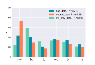
Figure 5: Genre distribution of top 1,000 sentences chosen by an active learning algorithm

Comparisons of selection algorithms   We empirically compare selection algorithms proposed in Section 4, as well as uniformly random baseline (RAND). All algorithms start with an identical 1% of original training data and a randomly initialized model. In each round, every algorithm chooses sentences from the rest of the training data until 20,000 words have been selected, adding this data to its training set. We then update each model by stochastic gradient descent on its augmented training dataset for 50 passes. We evaluate the performance of algorithm by its F1 score on the test dataset.

Figure 4 shows the results. All active learning algorithms perform significantly better than the random baseline. Among active learners, MNLP and BALD slightly outperformed traditional LC in early rounds. Note that MNLP is computationally more efficient than BALD, since it only requires a single forward pass on the unlabeled dataset to compute uncertainty scores, whereas BALD requires multiple forward passes. Impressively, active learning algorithms achieve 99% performance of the best deep model trained on full data using only 24.9% of the training data on the English dataset and 30.1% on Chinese. Also, 12.0% and 16.9% of training data were enough for deep active learning algorithms to surpass the performance of the shallow models from Pradhan et al. (2013) trained on the full training data. We repeated the experiment eight times and confirmed that the trend is replicated across multiple runs; see Appendix B for details.

Detection of under-explored genres   To better understand how active learning algorithms choose informative examples, we designed the following experiment. The OntoNotes datasets consist of six genres: broadcast conversation (bc), braodcast news (bn), magazine genre (mz), newswire (nw), telephone conversation (tc), weblogs (wb). We created three training datasets: half-data, which contains random 50% of the original training data, nw-data, which contains sentences only from newswire (51.5% of words in the original data), and no-nw-data, which is the complement of nw-data. Then, we trained CNN-CNN-LSTM model on each dataset. The model trained on half-data achieved 85.10 F1, significantly outperforming others trained on biased datasets (no-nw-data: 81.49, nw-only-data: 82.08). This showed the importance of good genre coverage in training data. Then, we analyzed the genre distribution of 1,000 sentences MNLP chose for each model (see Figure 5). For no-nw-data, the algorithm chose many more newswire (nw) sentences than it did for unbiased half-data (367 vs. 217). On the other hand, it undersampled newswire sentences for nw-only-data and increased the proportion of broadcast news and telephone conversation, which are genres distant from newswire. Impressively, although we did not provide the genre of sentences to the algorithm, it was able to automatically detect underexplored genres.

6 Conclusion

We proposed an efficient model for NER tasks which gives high performances on well-established datasets. Further, we use deep active learning algorithms for NER and empirically demonstrated that they achieve state-of-the-art performance with much less data than models trained in the standard supervised fashion.

Appendix A Effect of Beam Size on LSTM Decoder

One potential concern when decoding with an LSTM decoder as compared to using a CRF decoder is that finding the best sequence of labels that maximizes the probability $\mathbb{P}\left[t_{2},t_{3},\ldots,t_{n-1}\mid\left\{\mathbf{h}_{i}^{\text{Enc}}\right\}\right]$ is computationally intractable. In practice, however, we find that simple greedy decoding, i.e., beam search with beam size 1, works surprisingly well. Table 5 shows how changing the beam size of decoder affects the performance of the model. It can be seen that the performance of the model changes very little with respect to the beam size. Beam search with size 2 is marginally better than greedy decoding, and further increasing the beam size did not help at all. Moreover, we note that while it may be computationally efficient to pick the most likely tag sequence given a CRF encoder, the LSTM decoder may give more accurate predictions, owing to it’s greater representational power and ability to model long-range dependencies. Thus even if we do not always choose the most probable tag sequence from the LSTM, we can still outperform the CRF (as our experiments demonstrate).

Beam Size	F1
1	87.26
2	87.34
4	87.33
8	87.33
16	87.33

Table 5: Effect of beam size in LSTM decoder. We used a single LSTM-LSTM-LSTM model, and evaluated on OntoNotes 5.0 English dataset.

Appendix B Learning Curve in Active Learning Experiments across Multiple Runs

In order to understand the variability of learning curves in Figure 4(a) across experiments, we repeated the active learning experiment on OntoNotes-5.0 English eight times, each of which started with different initial dataset chosen randomly. Figure 6 shows the result in first nine rounds of labeled data acquisition. While MNLP, LC and BALD are all competitive against each other, there is a noticeable trend that MNLP and BALD outperforms LC in early rounds of data acquisition.

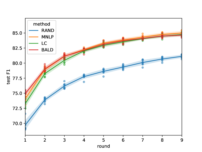
Figure 6: Test F1 score in first nine rounds of labeled data acquisition on OntoNotes-5.0 English dataset across multiple runs of the active learning experiment. The experiment was repeated eight times, with different initial dataset. Error bars indicates standard deviation, and dots indicate individual observation.

Appendix C Representativeness-based active learning

Consider that the confidence of the model can help to distinguish between hard and easy samples. Thus, sampling examples where the model is uncertain might save us from sampling too heavily from regions where the model is already proficient. But intuitively, when we query a batch of examples in each round, we might want to guard against querying examples that are too similar to each other, thus collecting redundant information. We also might worry that a purely uncertainty-based approach would oversample outliers. Thus we explore techniques to guard against these problems by selecting a set of samples that is representative of the dataset. Following Wei et al. (2015), we express the problem of maximizing representativeness of a labeled set as a submodular optimization problem, and provide an efficient streaming algorithm adapted to use a constraint suitable to the NER task. We also provide some with theoretical guarantees.

Submodular utility function

In order to reason about the similarity between samples, we first embed each sample $i$ into a fixed-dimensional euclidean space as a vector $\mathbf{x}_{i}$. We consider two embedding methods: 1) the average of pre-trained word embeddings, $\frac{1}{n}\sum_{t=1}^{n}\mathbf{w}_{t}^{\text{emb}}$, which can be efficiently computed without training of the NER model, and 2) the average of activation maps at the topmost layer of the encoder $\frac{1}{n}\sum_{t=1}^{n}\mathbf{h}_{t}^{\text{Enc}}$, an embedding which might be better suited to the context of the NER task. Then, we consider the following options for defining similarity scores $w(i,j)$ between each pair of samples $i$ and $j$: $w(i,j)=d-\|x^{i}-x^{j}\|_{p}$ where $d=\max_{i,j\in\mathbb{X}}\|x^{i}-x^{j}\|_{p}$ for $p=1,2$ which corresponds to closeness in $L_{1}$ and $L_{2}$ distance (Wei et al., 2015), and $w(i,j)=1+\frac{x_{i}\cdot x_{j}}{\|x_{i}\|\cdot\|x_{j}\|}$, which corresponds to cosine similarity.

Now, we formally define the utility function for labeling new samples. Denote $\mathbb{X}$ as the set of all samples which can be partitioned into two disjoint sets $\mathbb{X}^{\texttt{L}}$, $\mathbb{X}^{\texttt{U}}$ representing labeled and unlabeled samples, respectively. Let $\mathbb{S}\subseteq\mathbb{X}^{\texttt{U}}$ be a subset of unlabeled samples, then, the utility of labeling the set is defined as follows:

$$f(\mathbb{S})=\sum_{i\in\mathbb{X}^{\texttt{U}}}\left[\max_{j\in\mathbb{S}\cup\mathbb{X}^{\texttt{L}}}w(i,j)-\max_{j\in\mathbb{X}^{\texttt{L}}}w(i,j)\right],$$ (5)

where the function measures incremental gain of similarity between the labeled set and the rest. Given such utility function $f(\cdot)$, choosing a set $\mathbb{S}$ that maximizes the function within the budget can be seen as a monotone submodular maximization problem under a knapsack constraint (Krause & Golovin, 2012):

$$\max_{\mathbb{S}\subseteq\mathbb{X}^{\texttt{U}},\sum_{e\in\mathbb{S}}k(\{e\})\leq K}f(\mathbb{S})$$ (6)

where $k(\mathbb{S})$ is the budget for the sample set $\mathbb{S}$, and $K$ is the total budget within each round. Note that we need to consider the knapsack constraint instead of the cardinality constraint used in the prior work (Wei et al., 2015), because the entire sentence needs to be labeled once selected and sequences of length confer different labeling costs.

Combination with uncertainty sampling

Representation-based sampling can benefit from uncertainty-based sampling in the following two ways. First, we can re-weight each sample in the utility function (5) to reflect current model’s uncertainty on it:

$$f_{w}(\mathbb{S})=\sum_{i}\mathtt{US}(i)\cdot\left[\max_{j\in\mathbb{S}\cup\mathbb{X}^{\texttt{L}}}w(i,j)-\max_{j\in\mathbb{X}^{\texttt{L}}}w(i,j)\right],$$ (7)

where $\mathtt{US}(i)$ is the uncertainty score on example $i$. Second, even with the state-of-the-art submodular optimization algorithms, the optimization problem (6) can be computationally intractable. To improve the computational efficiency, we restrict the set of unlabeled examples to top samples from uncertainty sampling within budget $t\cdot K$, where $t$ is a multiplication factor we set as $4$ in our experiments.

Streaming algorithm for sample selection

Algorithm 1 Representativeness-based Sampling

1:  Input: Samples $\{\mathbb{X}^{\texttt{U}},\mathbb{X}^{\texttt{L}}\}$, budget $K$, pretrained model $\mathbb{M}$ using $\mathbb{X}^{\texttt{L}}$

2:  while Test score of $\mathbb{M}$ less than $th$ do

3:     Rank $\mathbb{X}^{\texttt{U}}$ according to Sec. 4, $\tilde{\mathbb{X}}^{\texttt{U}}=$ top samples $\mathbb{S}$ within budget $t\cdot K$.

4:     Set $f$ according to (5) or (7)

5:     $\mathbb{S}=\mathsf{StreamSubmodMax}(f,\tilde{\mathbb{X}}^{\texttt{U}})$.

6:     $\{\tilde{\mathbb{X}}^{\texttt{U}},\mathbb{X}^{\texttt{L}}\}=\{\mathbb{X}^{\texttt{U}}-\mathbb{S},\mathbb{X}^{\texttt{L}}\cup\mathbb{S}\}$

7:     Train $\mathbb{M}$ with $\mathbb{X}^{\texttt{L}}$.

8:  Output: $\mathbb{M}$

Algorithm 2 StreamSubmodMax

1:  Input: Submodular function $g$, set $\tilde{\mathbb{X}}^{\texttt{U}}$

2:  $m=\max_{e\in\tilde{\mathbb{X}}^{\texttt{U}}}g(\{e\})/k(\{e\})$

3:  $O=\{(1+\epsilon)^{i}|i\in\mathbb{Z},(1+\epsilon)^{i}\in[m,Km]\}$

4:   $\mathbb{S}_{v}:=\emptyset,\forall v\in O$

5:  for $e$ in $\tilde{\mathbb{X}}^{\texttt{U}}$  do

6:     for  $v\in O$ and $k(\mathbb{S}_{v}\cup\{e\})\leq K$  do

7:        if $\Delta_{g}(e|\mathbb{S}_{v})\geq\frac{k(\{e\})(v/2-g(\mathbb{S}_{v}))}{K-k(\mathbb{S}_{v})}$  then

8:            $\mathbb{S}_{v}:=\mathbb{S}_{v}\cup\{e\}$

9:  Output: $\arg\max_{v\in O}f(\mathbb{S}_{v})$

Even with the reduction of candidates with uncertainty sampling, (6) is still a computationally challenging problem and requires careful design of optimization algorithms. Suppose $l$ is the number of samples we need to consider. In the simplistic case in which all the samples have the same length and thus the knapsack constraint degenerates to the cardinality constraint, the greedy algorithm (Nemhauser et al., 1978) has an $(1-1/e)$-approximation guarantee. However, it requires calculating the utility function $O(l^{2}n)$ times, where $n$ is the number of unlabeled samples. In practice, both $l$ and $n$ are large. Alternatively, we can use lazy evaluation to decrease the computation complexity to $O(ln)$ (Leskovec et al., 2007), but it requires an additional hyperparameter to be chosen in advance. Instead of greedily selecting elements in an offline fashion, we adopt the two-pass streaming algorithm of Badanidiyuru et al. (2014), whose complexity is $\tilde{O}(ln)$, and generalize it to the knapsack constraint (shown in Alg. 2). In the first pass, we calculate the maximum function value of a single element normalized by its weight, which gives an estimate of the optimal value. In the second pass, we create $O(\frac{1}{\epsilon}\log K)$ buckets and greedily update each of the bucket according to:

$$\Delta_{g}(e|\mathbb{S}_{v})\geq\frac{k(\{e\})(v/2-g(\mathbb{S}_{v}))}{K-k(\mathbb{S}_{v})},$$ (8)

where each bucket has a different value $v$, and $\Delta_{g}(e|\mathbb{S}_{v}):=g(\{e\}\cup\mathbb{S}_{v})-g(\mathbb{S}_{v})$ is the marginal improvement of submodular function $g$ when adding element $e$ to set $\mathbb{S}_{v}$. The whole pipeline of the active learning algorithm is shown in Alg. 1. The algorithm gives the following guarantee, which is proven in Appendix.

Theorem 1.

Alg. 2 gives a $\frac{(1-\epsilon)(1-\delta)}{2}$-approximation guarantee for (6), where $\delta=\max_{e\in\mathbb{S}}k(\{e\})/K$.

Proof sketch: The criterion (8) we use guarantees that each update we make is reasonably good. The set $\mathbb{S}_{v}$ stops updating when either the current budget is almost $K$, or any sample in the stream after we reach $\mathbb{S}_{v}$ does not provide enough marginal improvement. While it is easy to give guarantees when the budget is exhausted, it is unlikely to happen; we use a difference expression between current set $\mathbb{S}_{v}$ and the optimal set, and prove the gap between the two is under control.

In a practical label acquisition process, the budget we set for each round is usually much larger than the length of the longest sentence in the unlabeled set, making $\delta$ negligible. In our experiments, $\delta$ was around $0.01$.

References

- Andor et al. (2016) Daniel Andor, Chris Alberti, David Weiss, Aliaksei Severyn, Alessandro Presta, Kuzman Ganchev, Slav Petrov, and Michael Collins. Globally normalized transition-based neural networks. arXiv preprint arXiv:1603.06042, 2016.
- Awasthi et al. (2014) Pranjal Awasthi, Maria Florina Balcan, and Philip M Long. The power of localization for efficiently learning linear separators with noise. In Proceedings of the 46th Annual ACM Symposium on Theory of Computing, pp. 449–458. ACM, 2014.
- Badanidiyuru et al. (2014) Ashwinkumar Badanidiyuru, Baharan Mirzasoleiman, Amin Karbasi, and Andreas Krause. Streaming submodular maximization: Massive data summarization on the fly. In Proceedings of the 20th ACM SIGKDD international conference on Knowledge discovery and data mining, pp. 671–680. ACM, 2014.
- Balcan et al. (2009) Maria-Florina Balcan, Alina Beygelzimer, and John Langford. Agnostic active learning. Journal of Computer and System Sciences, 75(1):78–89, 2009.
- Beygelzimer et al. (2009) Alina Beygelzimer, Sanjoy Dasgupta, and John Langford. Importance weighted active learning. In Proceedings of the 26th annual international conference on machine learning, pp. 49–56. ACM, 2009.
- Bontcheva et al. (2017) Kalina Bontcheva, Leon Derczynski, and Ian Roberts. Crowdsourcing named entity recognition and entity linking corpora. In Handbook of Linguistic Annotation, pp. 875–892. Springer, 2017.
- Chiu & Nichols (2016) Jason PC Chiu and Eric Nichols. Named entity recognition with bidirectional lstm-cnns. Transactions of the Association for Computational Linguistics, 4:357–370, 2016.
- Collobert et al. (2011) Ronan Collobert, Jason Weston, Léon Bottou, Michael Karlen, Koray Kavukcuoglu, and Pavel Kuksa. Natural language processing (almost) from scratch. Journal of Machine Learning Research, 12(Aug):2493–2537, 2011.
- Culotta & McCallum (2005) Aron Culotta and Andrew McCallum. Reducing labeling effort for structured prediction tasks. In AAAI, volume 5, pp. 746–51, 2005.
- Damianou & Lawrence (2013) Andreas Damianou and Neil Lawrence. Deep gaussian processes. In Artificial Intelligence and Statistics, pp. 207–215, 2013.
- Dasgupta et al. (2005) Sanjoy Dasgupta, Adam Tauman Kalai, and Claire Monteleoni. Analysis of perceptron-based active learning. In International Conference on Computational Learning Theory, pp. 249–263. Springer, 2005.
- Gal & Ghahramani (2016) Yarin Gal and Zoubin Ghahramani. A theoretically grounded application of dropout in recurrent neural networks. In Advances in Neural Information Processing Systems, pp. 1019–1027, 2016.
- Gal et al. (2017) Yarin Gal, Riashat Islam, and Zoubin Ghahramani. Deep bayesian active learning with image data. arXiv preprint arXiv:1703.02910, 2017.
- Graff & Cieri (2003) David Graff and Christopher Cieri. English gigaword, ldc catalog no. LDC2003T05. Linguistic Data Consortium, University of Pennsylvania, 2003.
- He et al. (2016) Kaiming He, Xiangyu Zhang, Shaoqing Ren, and Jian Sun. Deep residual learning for image recognition. In Proceedings of the IEEE Conference on Computer Vision and Pattern Recognition, pp. 770–778, 2016.
- Hinton et al. (2012) Geoffrey Hinton, Li Deng, Dong Yu, George E Dahl, Abdel-rahman Mohamed, Navdeep Jaitly, Andrew Senior, Vincent Vanhoucke, Patrick Nguyen, Tara N Sainath, et al. Deep neural networks for acoustic modeling in speech recognition: The shared views of four research groups. IEEE Signal Processing Magazine, 29(6):82–97, 2012.
- Hochreiter & Schmidhuber (1997) Sepp Hochreiter and Jürgen Schmidhuber. Long short-term memory. Neural computation, 9(8):1735–1780, 1997.
- Huang et al. (2015) Zhiheng Huang, Wei Xu, and Kai Yu. Bidirectional lstm-crf models for sequence tagging. arXiv preprint arXiv:1508.01991, 2015.
- Kendall & Gal (2017) Alex Kendall and Yarin Gal. What uncertainties do we need in bayesian deep learning for computer vision? arXiv preprint arXiv:1703.04977, 2017.
- Kilicoglu et al. (2016) Halil Kilicoglu, Asma Ben Abacha, Yassine Mrabet, Kirk Roberts, Laritza Rodriguez, Sonya E Shooshan, and Dina Demner-Fushman. Annotating named entities in consumer health questions. In LREC, 2016.
- Kim (2014) Yoon Kim. Convolutional neural networks for sentence classification. arXiv preprint arXiv:1408.5882, 2014.
- Krause & Golovin (2012) Andreas Krause and Daniel Golovin. Submodular function maximization. Tractability: Practical Approaches to Hard Problems, 3(19):8, 2012.
- Krizhevsky et al. (2012) Alex Krizhevsky, Ilya Sutskever, and Geoffrey E Hinton. Imagenet classification with deep convolutional neural networks. In Advances in neural information processing systems, pp. 1097–1105, 2012.
- Lafferty et al. (2001) John Lafferty, Andrew McCallum, Fernando Pereira, et al. Conditional random fields: Probabilistic models for segmenting and labeling sequence data. In Proceedings of the eighteenth international conference on machine learning, ICML, volume 1, pp. 282–289, 2001.
- Lample et al. (2016) Guillaume Lample, Miguel Ballesteros, Sandeep Subramanian, Kazuya Kawakami, and Chris Dyer. Neural architectures for named entity recognition. In Proceedings of NAACL-HLT, pp. 260–270, 2016.
- LeCun et al. (1995) Yann LeCun, Yoshua Bengio, et al. Convolutional networks for images, speech, and time series. The handbook of brain theory and neural networks, 3361(10):1995, 1995.
- Leskovec et al. (2007) Jure Leskovec, Andreas Krause, Carlos Guestrin, Christos Faloutsos, Jeanne VanBriesen, and Natalie Glance. Cost-effective outbreak detection in networks. In Proceedings of the 13th ACM SIGKDD international conference on Knowledge discovery and data mining, pp. 420–429. ACM, 2007.
- Lewis & Gale (1994) David D Lewis and William A Gale. A sequential algorithm for training text classifiers. In Proceedings of the 17th annual international ACM SIGIR conference on Research and development in information retrieval, pp. 3–12. Springer-Verlag New York, Inc., 1994.
- Ling et al. (2015) Wang Ling, Chris Dyer, Alan Black, and Isabel Trancoso. Two/too simple adaptations of word2vec for syntax problems. In Proceedings of the 2015 Conference of the North American Chapter of the Association for Computational Linguistics: Human Language Technologies. Association for Computational Linguistics, 2015.
- Manning (2016) Christopher D Manning. Computational linguistics and deep learning. Computational Linguistics, 2016.
- Mesnil et al. (2013) Grégoire Mesnil, Xiaodong He, Li Deng, and Yoshua Bengio. Investigation of recurrent-neural-network architectures and learning methods for spoken language understanding. In Interspeech, pp. 3771–3775, 2013.
- Mikolov et al. (2013) Tomas Mikolov, Ilya Sutskever, Kai Chen, Greg S Corrado, and Jeff Dean. Distributed representations of words and phrases and their compositionality. In Advances in neural information processing systems, pp. 3111–3119, 2013.
- Nair & Hinton (2010) Vinod Nair and Geoffrey E Hinton. Rectified linear units improve restricted boltzmann machines. In Proceedings of the 27th international conference on machine learning (ICML-10), pp. 807–814, 2010.
- Nemhauser et al. (1978) George L Nemhauser, Laurence A Wolsey, and Marshall L Fisher. An analysis of approximations for maximizing submodular set functions—i. Mathematical Programming, 14(1):265–294, 1978.
- Nguyen et al. (2016) Thien Huu Nguyen, Avirup Sil, Georgiana Dinu, and Radu Florian. Toward mention detection robustness with recurrent neural networks. arXiv preprint arXiv:1602.07749, 2016.
- Olsson (2009) Fredrik Olsson. A literature survey of active machine learning in the context of natural language processing. 2009.
- Pradhan et al. (2013) Sameer Pradhan, Alessandro Moschitti, Nianwen Xue, Hwee Tou Ng, Anders Björkelund, Olga Uryupina, Yuchen Zhang, and Zhi Zhong. Towards robust linguistic analysis using ontonotes. In CoNLL, pp. 143–152, 2013.
- Reimers & Gurevych (2017) Nils Reimers and Iryna Gurevych. Reporting score distributions makes a difference: Performance study of lstm-networks for sequence tagging. In Proceedings of the 2017 Conference on Empirical Methods in Natural Language Processing, pp. 338–348, 2017.
- Settles (2010) Burr Settles. Active learning literature survey. University of Wisconsin, Madison, 52(55-66):11, 2010.
- Settles & Craven (2008) Burr Settles and Mark Craven. An analysis of active learning strategies for sequence labeling tasks. In Proceedings of the conference on empirical methods in natural language processing, pp. 1070–1079. Association for Computational Linguistics, 2008.
- Shen et al. (2004) Dan Shen, Jie Zhang, Jian Su, Guodong Zhou, and Chew-Lim Tan. Multi-criteria-based active learning for named entity recognition. In Proceedings of the 42nd Annual Meeting on Association for Computational Linguistics, pp. 589. Association for Computational Linguistics, 2004.
- Srivastava et al. (2014) Nitish Srivastava, Geoffrey E Hinton, Alex Krizhevsky, Ilya Sutskever, and Ruslan Salakhutdinov. Dropout a simple way to prevent neural networks from overfitting. Journal of Machine Learning Research, 15(1):1929–1958, 2014.
- Strubell et al. (2017) Emma Strubell, Patrick Verga, David Belanger, and Andrew McCallum. Fast and accurate entity recognition with iterated dilated convolutions. In Proceedings of the 2017 Conference on Empirical Methods in Natural Language Processing, pp. 2660–2670, 2017.
- Tjong Kim Sang & De Meulder (2003) Erik F Tjong Kim Sang and Fien De Meulder. Introduction to the conll-2003 shared task: Language-independent named entity recognition. In Proceedings of the seventh conference on Natural language learning at HLT-NAACL 2003-Volume 4, pp. 142–147. Association for Computational Linguistics, 2003.
- Tong & Koller (2001) Simon Tong and Daphne Koller. Support vector machine active learning with applications to text classification. Journal of machine learning research, 2(Nov):45–66, 2001.
- Wang et al. (2016) Keze Wang, Dongyu Zhang, Ya Li, Ruimao Zhang, and Liang Lin. Cost-effective active learning for deep image classification. IEEE Transactions on Circuits and Systems for Video Technology, 2016.
- Wei et al. (2015) Kai Wei, Rishabh Iyer, and Jeff Bilmes. Submodularity in data subset selection and active learning. In Proceedings of the 32nd International Conference on Machine Learning (ICML-15), pp. 1954–1963, 2015.
- Yan & Zhang (2017) Songbai Yan and Chicheng Zhang. Revisiting perceptron: Efficient and label-optimal active learning of halfspaces. arXiv preprint arXiv:1702.05581, 2017.
- Yang et al. (2016) Zhilin Yang, Ruslan Salakhutdinov, and William Cohen. Multi-task cross-lingual sequence tagging from scratch. arXiv preprint arXiv:1603.06270, 2016.
- Zhai et al. (2017) Feifei Zhai, Saloni Potdar, Bing Xiang, and Bowen Zhou. Neural models for sequence chunking. In AAAI, pp. 3365–3371, 2017.
- Zhang et al. (2017) Ye Zhang, Matthew Lease, and Byron C Wallace. Active discriminative text representation learning. In AAAI, pp. 3386–3392, 2017.