Scaling of Lyapunov Exponents in Homogeneous Isotropic Turbulence

Abstract

Lyapunov exponents measure the average exponential growth rate of typical linear perturbations in a chaotic system, and the inverse of the largest exponent is a measure of the time horizon over which the evolution of the system can be predicted. Here, Lyapunov exponents are determined in forced homogeneous isotropic turbulence for a range of Reynolds numbers. Results show that the maximum exponent increases with Reynolds number faster than the inverse Kolmogorov time scale, suggesting that the instability processes may be acting on length and time scales smaller than Kolmogorov scales. Analysis of the linear disturbance used to compute the Lyapunov exponent, and its instantaneous growth, show that the instabilities do, as expected, act on the smallest eddies, and that at any time, there are many sites of local instabilities.

I Introduction

One of the defining characteristics of turbulence is that it is unstable, with small perturbations to the velocity growing rapidly. Indeed, turbulent flows in closed domains appear to be chaotic dynamical systems Keefe et al. (1992). The result is that the evolution of the detailed turbulent fluctuations can only be predicted for a finite time into the future, due to the exponential growth of errors. In a chaotic system, this prediction horizon is inversely proportional to the largest Lyapunov exponent of the system, which is the average exponential growth rate of typical linear perturbations. The maximum Lyapunov exponent $\bar{\gamma}$ is commonly used to characterize the chaotic nature of a dynamical system Eckmann and Ruelle (1985). In a turbulent flow, the maximum Lyapunov exponent is thus a measure of the strength of the instabilities that underlie the turbulence, and its inverse defines the time scale over which the turbulence fluctuations can be meaningfully predicted.

Lyapunov exponents in chaotic fluid flows have been estimated experimentally since the work of Swinney Wolf et al. (1985), using indirect methods. In numerical simulations, however, Lyapunov exponents can be determined directly by computing the evolution of linear perturbations. This has been done for weakly turbulent Taylor Couette flow Vastano and Moser (1991) and very low Reynolds number planar Poiseuille flow Keefe et al. (1992). Remarkably, to the authors’ knowledge, Lyapunov exponents have not been determined for isotropic turbulence, a shortcoming corrected in this paper.

Homogeneous isotropic turbulence is an idealized turbulent flow that has been extensively studied both experimentally Mydlarski and Warhaft (1996); Comte-Bellot and Corrsin (1971, 1966) and using numerical simulations Rogallo (1981); Vincent and Meneguzzi (1991); Jiménez et al. (1993); Chen and Shan (1992). It is valuable as a model for the small scales of high Reynolds number turbulence away from walls Durbin and Reif (2011). It has been speculated that in isotropic turbulence, the maximum Lyapunov exponent scales with the inverse Kolmogorov time scale Crisanti et al. (1993), suggesting that the dominant instabilities occur at Kolmogorov length scales as well. If true, then a study of the maximum Lyapunov exponent and the associated instabilities in homogeneous isotropic turbulence will be applicable to a wide range of flows.

This paper focuses on how the maximum Lyapunov exponent and hence the predictability time horizon scale with Reynolds number and computational domain size of a numerically simulated homogeneous isotropic turbulence. The speculation that $\bar{\gamma}$ should scale as the inverse Kolmogorov time scale $\tau_{\eta}$ Crisanti et al. (1993) is in agreement with an estimate from a shell model Aurell et al. (1996). However, this scaling has not been directly tested in direct numerical simulations.

In addition, in the process of computing the maximum Lyapunov exponent in a direct numerical simulation, one necessarily computes the linear disturbance that is most unstable (on average). This can be used in the short-time Lyapunov exponent analysis, as introduced in Vastano and Moser (1991), to characterize the nature of the instabilities. This will be pursued here for isotropic turbulence.

The remainder of this paper includes a brief review of Lyapunov exponents and how they are computed in numerical simulations (section II) followed by a description of the direct numerical simulations studied here (section III). The results of a scaling study of the Lyapunov exponents are given in section IV, and a short-time Lyapunov exponent analysis is presented in section V, followed by concluding remarks in section VI.

II Lyapunov Exponent Analysis

Two important characteristics of chaotic dynamical systems for the purposes of the current study are that 1) solutions evolve toward a stable attractor, and 2) solution trajectories on the attractor are unstable so that near-by trajectories diverge exponentially. The rate of this exponential divergence is characterized by the Lyapunov exponents, whose characteristics are recalled briefly here. Further details can be found in Vastano and Moser (1991). In addition, the use of Lyapunov exponents in the analysis presented in the paper is described.

II.1 Evolution of Linear Perturbations

Consider a solution trajectory $u(t)$ of a chaotic system. The solution will evolve toward an attracting set in phase space (the attractor); in turbulence this corresponds to the solution evolving to a statistically stationary state. Let $u(t_{0})$ at some arbitrary starting time $t_{0}$ be on the attractor, and consider an infinitesimal perturbation $\delta u(t_{0})$ of the solution at time $t_{0}$, and its evolution in time. The Lyapunov exponents describe the growth or decay of the magnitude of $\delta u$. In particular, the multiplicative ergodic theorem Oseledec (1968) implies that the limit

$$\bar{\gamma}=\lim_{t\rightarrow\infty}\frac{1}{t}\log\left(\frac{\|\delta u(t)\|}{\|\delta u(t_{0})\|}\right)$$ (1)

exists and $\bar{\gamma}$ is called a Lyapunov exponent. There is a spectrum of possible Lyapunov exponents, depending on the solution $u(t_{0})$ and the perturbation $\delta u(t_{0})$ at the starting time. However, for almost all $\delta u(t_{0})$, $\bar{\gamma}=\gamma_{1}$ the largest Lyapunov exponent, and, due to round-off error and other sources of noise, in practical computations, $\bar{\gamma}=\gamma_{1}$ for all $\delta u(t_{0})$. Furthermore, the Lyapunov spectrum ($\gamma_{1}>\gamma_{2}>\gamma_{2}>\cdots$) does not depend on $u(t_{0})$; it is instead a property of the dynamical system. See the review by Eckmann et al. Eckmann and Ruelle (1985) for an introduction to the theory.

In addition, in practical computations as discussed above, we expect that in the limit $t\rightarrow\infty$

$$\frac{\delta u(t)}{\|\delta u(t)\|}\rightarrow\overline{\delta u}(u(t))\qquad\mbox{and}\qquad\frac{1}{\|\delta u(t)\|}\frac{d\|\delta u(t)\|}{dt}\rightarrow\gamma^{\prime}(u(t))$$ (2)

where $\overline{\delta u}$ and $\gamma^{\prime}$ depend only on the solution at $t$, and not on the starting conditions $u(t_{0})$ and $\delta u(t_{0})$. The perturbation $\overline{\delta u}$ is the disturbance that grows most rapidly in the long run, growing at the average exponential rate $\bar{\gamma}$. It is defined by the fact that it’s long-time average growth rate forward in time is $\bar{\gamma}$ and when the evolution is backward in time the long-time average growth rate is $-\bar{\gamma}$. The short-time Lyapunov exponent $\gamma^{\prime}$ is simply the instantaneous exponential growth rate of $\overline{\delta u}$.

Because $\gamma^{\prime}$ and $\overline{\delta u}$ depend only on the solution at the current time, they can be used as diagnostics for the instabilities responsible for a system being chaotic. In particular, when $\gamma^{\prime}$ is large, the underlying system is particularly unstable, and at that time the Lyapunov disturbance $\overline{\delta u}$ is rapidly growing. Thus by seeking out times when $\gamma^{\prime}$ is large, and by analyzing the solution $u$ and the Lyapunov disturbance $\overline{\delta u}$ at that time, we can characterize the important instabilities. This is the short-time Lyapunov exponent analysis described by Vastano & Moser Vastano and Moser (1991).

In this paper we will be concerned with the scaling of $\bar{\gamma}$ with Reynolds number and with the chaotic instabilities revealed by short-time Lyapunov exponent analysis.

III Simulations

To simulate the base field, we solve the three-dimensional incompressible Navier-Stokes equations on a cube of dimension $L=2\pi$, with periodic boundary conditions, to obtain a computational approximation of homogeneous isotropic turbulence. Turbulence is maintained by introducing a forcing term to the Navier-Stokes equations which only acts at large scales. The forcing formulation is described in section III.1. The Navier-Stokes equations are solved using a Fourier-Galerkin spatial discretization with $N$ modes in each direction, and the vorticity formulation of Kim et al. Kim et al. (1987). This formulation has the advantage of exactly satisfying the continuity constraint while eliminating the pressure term. A low-storage explicit third-order Runge-Kutta scheme Spalart et al. (1991) is used for time evolution. The simulations are performed using a modified version of the channel flow code PoongBack Lee et al. (2013, 2014).

To compute the Lyapunov exponents, we compute the growth rate of a linear perturbation added to the base field. This perturbation satisfies the linearized Navier-Stokes equations:

$$\frac{\partial\delta u_{i}}{\partial t}+\frac{\partial}{\partial x_{j}}(u_{j}\delta u_{i}+\delta u_{j}u_{i})=-\frac{\partial\delta p}{\partial x_{i}}+\frac{1}{Re}\nabla^{2}\delta u_{i}$$ (3)

$$\partial_{i}\delta u_{i}=0,$$ (4)

where $u_{i}$ is the base field and $\delta u_{i}$ is the disturbance field. The disturbance equations are solved using the same numerical scheme as the Navier-Stokes equations. Note that the forcing is applied only to the base field and not the perturbation. The implementation of both the base and disturbance field solvers were verified using the method of manufactured solutions.

III.1 Forcing

The goal of the forcing is to inject energy into the large-scale turbulence so that the isotropic turbulence will be stationary. Forcing is applied to Fourier modes with wavenumber magnitudes in a specified range, and is designed to produce a specified rate of energy injection (forcing power), which, when the system is stationary, will be the dissipation rate. By specifying the wavenumber range being forced, forcing power and viscosity, the integral scale, turbulent kinetic energy and Reynolds number can be controlled.

The energy injection is accomplished by the introduction of a forcing term $f_{i}$ to the Navier Stokes equations:

$$\frac{\partial u_{i}}{\partial t}+\frac{\partial u_{i}u_{j}}{\partial x_{j}}=-\frac{\partial p}{\partial x_{i}}+\frac{1}{Re}\nabla^{2}u_{i}+f_{i}$$ (5)

$$\partial_{i}u_{i}=0.$$ (6)

Following Spalart et al. (1991), in the Fourier spectral method used here, the Fourier transform of the forcing $\hat{f}_{i}$ is specified in terms of the velocity Fourier transform $\hat{u}_{i}$ as

$$\hat{f}_{i}(\mathbf{k})=\alpha|\mathbf{k}|^{2}\hat{u}_{i}(\mathbf{k}).$$ (7)

Given that $u_{i}$ is a Navier-Stokes solution, $f_{i}$ is guaranteed to be divergence-free. The coefficient $\alpha$ in the above is determined as a function of time so that the forcing power is the target dissipation rate $\epsilon_{T}$. Since the forcing is applied only to a range of wavenumbers, this yields

$$\alpha=\epsilon_{T}\begin{cases}{\displaystyle\epsilon_{T}\left(\sum_{k_{f_{\text{min}}}\leq|\mathbf{k}|\leq k_{f_{\text{max}}}}|\mathbf{k}|^{2}\hat{u}^{*}_{i}(\mathbf{k})\hat{u}_{i}(\mathbf{k})\right)^{-1}}&k_{f_{\text{min}}}\leq|\mathbf{k}|\leq k_{f_{\text{max}}}\\ 0&\text{otherwise}\end{cases}$$ (8)

where $\cdot^{*}$ denotes the complex conjugate, and $k_{f_{\text{min}}}$ and $k_{f_{\text{max}}}$ are the bounds on the range of wavenumbers being forced. In the Fourier transform of the Navier-Stokes equations, the viscous term has the same structure as $f_{i}$, so this forcing can be interpreted as a negative viscosity acting in the specified wavenumber range. The combined forcing and viscous term is then $-(\nu-\alpha)|\mathbf{k}|^{2}\hat{u}_{i}(\mathbf{k})$. In the numerical solution of the Navier-Stokes equations, this combined term is treated in the same way as the viscous term would be. Note that $f_{i}$ is just a nonlinear function of $u_{i}$, so there is no externally imposed stochasticity.

Case	$k_{f_{\text{min}}}$	$k_{f_{\text{max}}}$	$\nu$	$N$	$\mathcal{L}$	$Re_{\lambda}$	$T_{\rm avg}q/\cal{L}$
1	0	2	0.0235	64	1.43	37.92	455.2
2	0	2	0.0113	96	1.58	58.34	123.8
3	0	2	0.0056	128	1.67	85.68	118.0
4	0	2	0.0038	192	1.70	106.33	51.2
5	0	2	0.0026	256	1.77	130.43	51.3
6	0	2	0.0010	512	1.82	211.76	69.5
7	2	4	0.0093	128	0.71	37.74	277.1
8	4	8	0.0037	256	0.35	37.31	72.1

Table 1: Parameters defining the eight direct numerical simulations performed to study Lyapunov exponent scaling. Values of $\mathcal{L}$ are quoted in units in which the domain size is $2\pi$, and averaging times are normalized by eddy turnover time.

III.2 Simulation Cases

To investigate the scaling of the maximum Lyapunov exponent $\bar{\gamma}$ with both Reynolds number and the ratio of the computational domain size $L$ to the integral scale $\mathcal{L}$, eight simulations were performed. These are summarized in table 1. To study the scaling of $\bar{\gamma}$ with Reynolds number, six cases where simulated with the same forcing wavenumber range and $\epsilon_{T}$. This resulted in approximately the same integral scale in each case. The Reynolds number was manipulated by changing the viscosity. To study the potential variation of $\bar{\gamma}$ with domain size normalized by integral scale, the domain size was kept fixed at $2\pi$ and the integral scale was changed by adjusting the forced wavenumber range, while keeping the Reynolds number approximately fixed. In all cases $k_{\text{max}}\eta>1$, where $k_{\text{max}}$ is the maximum resolved wavenumber, and $\eta$ is the Kolmogorov scale. In a refinement study, this was found to be sufficient to obtain resolution independent values of $\bar{\gamma}$.

For each case, the simulations were run until the base solution became statistically steady and then the statistics were gathered by time averaging over a period $T_{\rm avg}$ as reported in table 1. The simulation was confirmed to be stationary by verifying the convergence of the viscous dissipation to $\epsilon_{T}$ and the statistical convergence rates of $q^{2}$ and $\bar{\gamma}$.

IV Scaling of Lyapunov Exponents

Of primary concern here is the dependence of the maximum Lyapunov exponent on the Reynolds number and on the domain size. To address this, the maximum Lyapunov exponent $\bar{\gamma}$, the integral scale ($\mathcal{L}$) and Reynolds number based on the Taylor micro-scale ($Re_{\lambda}$) are needed, along with their uncertainties. Based on the assumption of isotropy, the latter two were determined to be $\mathcal{L}=0.15q^{3}/\epsilon$ and $Re_{\lambda}=q^{2}\sqrt{5/(3\epsilon\nu)}$ Pope (2001). Thus the two statistical quantities that need to be computed from the DNS are $\bar{\gamma}$ and $q^{2}$. Both are determined as a time average over averaging time $T_{\rm avg}$ (see table 1), and the standard deviations $\sigma$ of the uncertainty due to finite averaging time were determined using the technique described by Oliver et al. (2014). The values of $\bar{\gamma}$, $q^{2}$ and their standard deviations are given in table 2. The standard deviations of the derived quantities $\mathcal{L}$ and $Re_{\lambda}$ are determined simply as $\sigma_{\mathcal{L}}=(0.225q/\epsilon)\sigma_{q^{2}}$ and $\sigma_{Re_{\lambda}}=\sqrt{5/(3\epsilon\nu)}\sigma_{q^{2}}$, where for $\sigma_{\mathcal{L}}$ it is assumed that $\sigma_{q^{2}}/q^{2}\ll 1$. Note that since for each simulation $\epsilon$ and $\nu$ are specified, there is no uncertainty in their values.

case	$q^{2}$	$\sigma_{q^{2}}$	$\bar{\gamma}\tau_{\eta}$	$\sigma_{\bar{\gamma}}\tau_{\eta}$
1	4.51	0.107	0.0922	0.0038
2	4.80	0.160	0.1075	0.0046
3	4.99	0.075	0.1177	0.0032
4	5.05	0.044	0.1231	0.0040
5	5.19	0.046	0.1304	0.0034
6	5.28	0.084	0.1599	0.0048
7	2.82	0.008	0.0941	0.0019
8	1.76	0.001	0.0945	0.0021

Table 2: Values of $q^{2}$ and the maximum Lyapunov exponent $\bar{\gamma}$, along with the standard deviation ($\sigma$) of the sampling uncertainty. Values of $q^{2}$ are quoted in units in which the domain size is $2\pi$ and $\epsilon=1$, and $\bar{\gamma}$ is normalized by the Kolmogorov time scale $\tau_{\eta}$.

Figure 1: Dependence of the Lyapunov exponent scaled in Kolmogorov units ($\bar{\gamma}\tau_{\eta}$) on (a) the Taylor scale Reynolds number $Re_{\lambda}$ and (b) the ratio of the integral scale to the domain size $\mathcal{L}/L$, from the data in table 2. The error bars on the data (in blue) represent one standard deviation. Also shown are the outputs of the models (9) (in red) calibrated with Bayesian inference, with the dark and light gray shading representing variations of one and two standard deviations respectively.

The dependence of the maximum Lyapunov exponent in Kolmogorov units on Reynolds number is shown in figure 1, including uncertainties expressed as the standard deviation. If the hypothesized scaling of the Lyapunov exponent on Kolmogorov time scale were correct, these data would, within their uncertainty, fall along a horizontal line. However, this does not appear to be the case. Indeed, $\bar{\gamma}\tau_{\eta}$ appears to be growing with $Re_{\lambda}$. Also, shown in figure 1 is the dependence of scaled Lyapunov exponent on domain size at constant Reynolds number. These data do appear to be consistent with the hypothesis that the Lyapunov exponent does not depend on the domain size.

To make these scaling observations quantitative, Bayesian inference is used to infer the coefficients $\alpha$ and $\beta$ in a scaling relationships of the form

$$\bar{\gamma}\tau_{\eta}=\alpha_{1}Re_{\lambda}^{\beta_{1}}\quad\mbox{and}\quad\bar{\gamma}\tau_{\eta}=\alpha_{2}(\mathcal{L}/L)^{\beta_{2}},$$ (9)

given the data and its uncertainties. These scaling relationships serve as the “model” for the inference. In Bayesian inference for this problem, the joint probability distribution $\pi(\alpha,\beta|{\bf d})$ of the parameters $\alpha$ and $\beta$ conditioned on data ${\bf d}$ (shown in table 1) is sought. Bayes’ theorem gives this conditional probability as:

$$\pi(\alpha,\beta|{\bf d})\propto\pi({\bf d}|\alpha,\beta)\pi(\alpha,\beta)$$ (10)

where $\pi({\bf d}|\alpha,\beta)$ is the likelihood and $\pi(\alpha,\beta)$ is the prior. The likelihood is the joint probability density for the observed quantities evaluated for the observed values of these quantities, as determined by the model with parameters $\alpha$ and $\beta$, and given the uncertainties in the data. The prior represents our prior knowledge about the parameters, independent of the data.

The data are statistical averages obtained from direct numerical simulations. The primary source of uncertainty in such data is statistical sampling error. The central limit theorem implies that in the limit of large samples, the uncertainty associated with sampling error is normally distributed with zero mean. Therefore, to formulate the likelihood, the data are assumed to have Gaussian uncertainty with standard deviations as reported in table 2. The probability distribution for the $i$th observation of the value of $\bar{\gamma}$ as predicted by the models is thus given by

$$\pi(\bar{\gamma}|\alpha,\beta,x_{i})=\frac{1}{\sigma_{\gamma_{i}}\sqrt{2\pi}}\exp\left[-\frac{(\bar{\gamma}-\alpha_{1}x_{i}^{\beta_{1}})^{2}}{2\sigma_{\gamma_{i}}^{2}}\right]$$ (11)

where $x_{i}$ is the independent variable ($Re_{\lambda i}$ or $\mathcal{L}_{i}/L$, depending on which scaling relation is being inferred) of the $i$th observation and $\sigma_{\gamma_{i}}$ is the standard deviation in $\bar{\gamma}$ associated with the $i$th observation. However, there are also uncertainties in the values of the independent variables $x$, as determined from the DNS, again with a Gaussian distribution and standard deviation for the $i$th observation of $\sigma_{x_{i}}$. In this case, the probability distribution of the independent variable $x$ given the observation $x_{i}$ is

$$\pi(x|x_{i})=\frac{1}{\sigma_{x_{i}}\sqrt{2\pi}}\exp\left[-\frac{(x-x_{i})^{2}}{2\sigma_{x_{i}}^{2}}\right].$$ (12)

The conditional distribution of $\bar{\gamma}$ given the parameters and the observed independent variable is then given by

$$\pi(\bar{\gamma}|\alpha,\beta,x_{i})=\int_{x}\pi(\gamma|\alpha,\beta,x)\pi(x|x_{i})\,dx.$$ (13)

Finally, to obtain the likelihood, (13) is evaluated at $\bar{\gamma}=\gamma_{i}$ and the uncertainties in each observation are assumed to be independent (an excellent assumption), yielding:

$$\pi({\bf d}|\alpha,\beta)=\prod_{i}\pi(\bar{\gamma}=\gamma_{i}|\alpha,\beta,x_{i}).$$ (14)

To inform the prior, we consider the range of time scales in the turbulence. The largest is the eddy turn-over time, which is proportional to $q^{2}/\epsilon$, and the smallest is the Kolmogorov time scale $\sqrt{\nu/\epsilon}$. The ratio of the turnover to the Kolmogorov times scales as $Re_{\lambda}$. Therefore, the Lyapunov exponent $\bar{\gamma}\tau_{\eta}$ scaling with the turn-over time would imply $\beta=-1$ and scaling with the Kolmogorov scale would imply $\beta=0$. However, theoretical arguments suggest that the Lyapunov exponent scales with the Kolmogorov time scale Crisanti et al. (1993) ($\beta=0$), and we need to allow for the possibility that this assessment may be in error in either direction. The bounds on the range of plausible values of $\beta$ were therefore extended to $-1\leq\beta\leq 1$, and a uniform distribution over this range was used as a prior for $\beta$. Somewhat arbitrarily, the same range was used for the $\beta$ prior in the domain size scaling relationship. The parameter $\alpha$ is a positive definite scaling parameter, and so following Jaynes Jaynes (2003), a Jeffries distribution $\pi(\alpha)\sim 1/\alpha$ is used as an (improper) prior. Finally, the priors for $\alpha$ and $\beta$ are independent so $\pi(\alpha,\beta)=\pi(\alpha)\pi(\beta)$.

Figure 2: Posterior PDFs for $\alpha_{1}$ and $\beta_{1}$ in the Reynolds number scaling model (9). Shown are the marginal distributions of both parameters along with contours of their joint distribution.

Figure 3: Posterior PDFs for $\alpha_{2}$ and $\beta_{2}$ in the domain size scaling model (9). Shown are the marginal distributions of both parameters along with contours of their joint distribution.

Given the likelihood and prior described above, and the data in Table 2, samples of the posterior distribution were obtained using a Markov-chain Monte Carlo (MCMC) algorithm Haario et al. (2006) as implemented in the QUESO library Prudencio and Schulz (2012); McDougall et al. (2015). The resulting samples were used to characterize the joint posterior distribution of $\alpha$ and $\beta$ for both the Reynolds number and domain size scaling model, as shown in figures 2 and 3. Notice in these figures that the joint distribution has probability mass concentrated in thin diagonally oriented regions, showing that uncertainty in $\alpha$ and $\beta$ are highly correlated. Indeed, the uncertainty in the $\beta$’s is as large as it is because changes in $\beta$ can be compensated for by changes in $\alpha$ so that the model still fits the data. The MCMC samples were also used to determine the uncertainty in the model predictions for the Lyapunov exponent as a function of Reynolds number and domain size, with the results plotted in figure 1, along with the data. From this, it is clear that the scaling models as calibrated are consistent with the data and their uncertainty.

The marginal posterior distribution for $\beta$ in the Reynolds number scaling relation shows that the most likely values of $\beta$ are between about $1/4$ and $1/3$, with the possibility that the value is zero essentially precluded. This is remarkable since it suggests instability time scales that will become increasingly faster than Kolmogorov with increasing Reynolds number. The origin of this fast time scale is currently unclear. One possibility to consider is that this fast instability time scale arises as an artifact of the time discretization of the DNS. However the DNS time step in Kolmogorov units $\Delta t/\tau_{\eta}\sim Re_{\lambda}^{-1/2}$, so if the Lyapunov exponent were scaling with the DNS time step, $\beta$ would be 1/2, which is also essentially precluded by the posterior distribution. The time discretization thus appears to be an unlikely origin of the observed Reynolds number scaling. This was also verified by running a time refinement study where $\bar{\gamma}$ was found to be invariant to changing $\Delta t$.

As with the time step, interest in the computational domain size arises because of concern that computational artifacts not impact our Lyapunov exponent analysis. The posterior distribution of $\beta$ in the domain size scaling relationship (figure 3) shows that $\beta=0$ is highly likely, with the most probable values of $\beta$ ranging from -0.05 to 0.05. If there is an effect of the domain size, the data indicates that it is extremely weak. It therefore appears that the Lyapunov exponent Reynolds number scaling discussed above and the short-time Lyapunov exponent analysis presented in section V are unaffected by finite domain size effects.

V Short-Time Lyapunov Exponent Analysis

As discussed in section II, both the disturbance field ($\delta u$) used to compute the Lyapunov exponent and its instantaneous exponential growth rate ($\gamma^{\prime}$) depend only on the instantaneous Navier-Stokes velocity $u$, not on the initial disturbance. In short-time Lyapunov exponent analysis, we study $\gamma^{\prime}$ and $\delta u$ to learn about the instabilities responsible for the chaotic nature of turbulence.

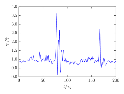
First, consider the time evolution of the exponential growth rate $\gamma^{\prime}$, which is shown in figure 4 for $Re_{\lambda}=37$ and 210 (cases 1 and 6 respectively), normalized by $\bar{\gamma}$. Note that in both cases $\gamma^{\prime}$ takes large excursions from the mean, of order 3 times the mean value. However, the variations in $\gamma^{\prime}$ occur on a much shorter time scale and the large excursions seem to occur more often in the high Reynolds number case. The time scale on which $\gamma^{\prime}$ varies appears to decrease somewhat faster than the Kolmogorov time scale with increasing Reynolds number, as when plotted against $t/\tau_{\eta}$, $\gamma^{\prime}$ still varies faster for case 6 (figure 5). At the same Reynolds number (cases 1 and case 8), the variability of $\gamma^{\prime}$ decreases sharply with increasing relative computational domain size $L/\mathcal{L}$. The fact that the time scale of the instability, as measured by the Lyapunov exponent, decreases faster than the Kolmogorov time scale suggests that the instability processes are acting at spatial scales near the Kolmogorov scale. In this case, a simulation with a larger domain size relative to intrinsic turbulence length scales would include a larger sample of local unstable turbulent flow features, resulting in smaller variability in $\gamma^{\prime}$. In comparing case 8 with case 1, the relative volume increases by a factor 64, suggesting that the variability of $\gamma^{\prime}$ should be about a factor of 8 smaller in case 8 than in case 1, which is indeed consistent with the data.

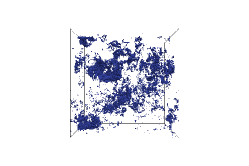
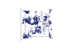
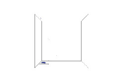
At the peaks in $\gamma^{\prime}$, the growth of the disturbance energy is particularly rapid, and the question naturally arises as to what is special about these times. To investigate this, the spatial distribution of the magnitude of the disturbance energy density is visualized in figure 6 at three times, just before the beginning of a peak in $\gamma^{\prime}$, a time half way up that peak and at the peak ($tq/\mathcal{L}=9.58$, 9.85 and 9.89 in figure 4). Notice that before the rapid growth of $\gamma^{\prime}$ into the peak, the energy in the disturbance field is broadly distributed across the spatial domain. Half way up the peak, the distribution is much more spotty, and finally at the peak, the disturbance energy is primarily focused in a small region, appearing in the lower left corner of figure 6(c). The contour levels in these images were chosen so that the contours enclose 60% of the disturbance energy, implying that 60% of the disturbance energy is concentrated in the small feature in the lower left of figure 6(c). Another indication of the dominance of the disturbance feature in figure 6(c) is that the contour level needed to enclose 60% of the energy is about 2500 times the mean disturbance energy density, while in figure 6(a) the contour is only about 15 times the mean. Clearly the growth of the disturbance field in this concentrated area is responsible for the peak in $\gamma^{\prime}$. However, the spatially local exponential growth rate of the disturbance energy $|\delta u|^{-2}\,\partial|\delta u|^{2}/\partial t$ is not particularly large there, large values of this quantity are distributed broadly across the spatial domain. It seems, then, that the large peak in $\gamma^{\prime}$ is due to a local disturbance that is able to grow over an extended time until it dominates the disturbance energy, so that the disturbance is localized in a region of relatively large growth rate. This is presumably unusual because it requires that the local unstable flow structure responsible for the disturbance growth persists for a long time.

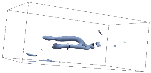
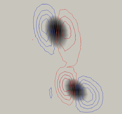
It is of interest to investigate the turbulent flow structures responsible for the large localized disturbance energy at the peak in $\gamma^{\prime}$. In the region where $\delta u$ is localized, the base field exhibits a pair of co-rotating vortex tubes (figure 7). As shown in figure 8, the disturbance vorticity is localized on the vortex tubes, with regions of opposite signed disturbance vorticity to one side or the other of each vortex tube. This disturbance, when added to the base field would have the effect of displacing each vortex tube along the line between the positive and negative peaks in the disturbance vorticity associated with each tube. The instability then appears to be one associated with slowing (speeding up) the co-rotation of the vortex tubes while they move away from (toward) each other. Note that the disturbance equations, being linear and homogeneous, are invariant to a sign change, and so the sign of the vortex displacement is indeterminate. Such an instability of co-rotating vortices is reminiscent of the pairing instability in two-dimensional mixing layers.

(a) Case 1, $Re_{\lambda}=37$

(b) Case 8, $Re_{\lambda}=37$, large $L/\mathcal{L}$

(c) Case 6, $Re_{\lambda}=210$

(d) Case 6, $Re_{\lambda}=210$ (zoomed in)

Figure 4: Short-time Lyapunov exponent scaled by $\bar{\gamma}$. In (d), the time axis is expanded to zoom in on the peak indicated in (c), and symbols show the times at which the images in figure 6 were obtained.

(a) Case 1, $Re_{\lambda}=37$

(b) Case 6, $Re_{\lambda}=210$

Figure 5: Short-time Lyapunov exponent $\gamma^{\prime}/\bar{\gamma}$ with time scaled by $\tau_{\eta}$.

(a) $tq/\mathcal{L}=9.58$

(b) $tq/\mathcal{L}=9.85$

(c) $tq/\mathcal{L}=9.89$

Figure 6: Contour of the magnitude of $\delta u$ at three times leading up to the peak as indicated in figure 4 for $Re_{\lambda}=210$ (case 6). The contour shown is that at which 60% of the disturbance energy is enclosed by the contour. To achieve this, the contour levels are (a) 15, (b) 25, and (c) 2500 times the mean disturbance energy density.

Figure 7: Contour of the magnitude of the vorticity of the base field for $Re_{\lambda}=210$ (case 6) at the peak of $\gamma^{\prime}$ in the region where the disturbance field is localized (box highlighted in figure 6c) . The contour level is 9.2 times the square root of the mean enstrophy. The vortex tubes are co-rotating, with the direction of rotation indicated by the black arrow.

Figure 8: The magnitude of the vorticity (grayscale) and the disturbance vorticity component normal to the plane (contour lines) in a plane perpendicular to and in the middle of the vortex tubes shown in figure 7. For the disturbance vorticity, the red and blue contours are of opposite signs.

VI Conclusions

The results of the scaling study (section IV) show definitively that, at least over the Reynolds number range studied, the Lyapunov exponent does not scale like the inverse Kolmogorov time scale, as had been previously suggested Aurell et al. (1996). Instead, $\bar{\gamma}\tau_{\eta}$ increases with Reynolds number like $Re_{\lambda}^{\beta}$ for $\beta$ in the range from 1/4 to 1/3. Further note that the analysis of Aurell et al. Aurell et al. (1996) indicated that a correction for the intermittance of dissipation would yield $\beta<0$, also inconsistent with the current results. If positive $\beta$ scaling holds to much higher Reynolds numbers, it would be remarkable, as it would mean that there are instability processes that act on time scales shorter than Kolmogorov. However, in the highest Reynolds number ($Re_{\lambda}=210$) simulation performed here, $\bar{\gamma}\tau_{\eta}$ is still only 0.16. It is certainly possible that this Reynolds number dependence of $\bar{\gamma}\tau_{\eta}$ is a low Reynolds number effect, caused by insufficient scale separation between the large scales and the scales at which the instabilities act, and that the value will reach a plateau at some much higher Reynolds number. Clearly, this scaling behavior of the maximum Lyapunov exponent is worthy of further study. The current results suggest that the generally accepted and most obvious scaling is not correct, and that, unfortunately, turbulent fluctuations are even less predictable than previously thought.

The short-time analysis described in section V confirmed that the dominant instabilities in turbulence act on the smallest eddies. Further, at $Re_{\lambda}=210$, when the instantaneous disturbance growth rate was the largest (about 3 times the mean), the disturbance energy was highly localized, suggesting that it was a particular local instability that was responsible for the rapid growth at that time. However, this was not due to a particularly large local growth rate, as the logarithmic time derivative of the spatially local disturbance energy was equally large in regions spread throughout the domain. It may be that the localized instability we observed is not of particular importance, except that the underlying structure in the turbulent field was especially long-lived. None-the-less, studying it showed that one of the possible instability mechanisms acting in turbulence is reminiscent of pairing instabilities of co-rotating vortices, as in a mixing layer. In this, the short-time Lyapunov analysis pursued here appears to be a valuable tool for the study of the instabilities underlying turbulence.

References

- Aurell et al. [1996] E. Aurell, G. Boffetta, A. Crisanti, G. Paladin, and A. Vulpiani. Growth of noninfinitesimal perturbations in turbulence. Physical review letters, 77(7):1262, 1996.
- Chen and Shan [1992] S. Chen and X. Shan. High-resolution turbulent simulations using the connection machine-2. Computers in Physics, 6(6):643–646, 1992.
- Comte-Bellot and Corrsin [1966] G. Comte-Bellot and S. Corrsin. The use of a contraction to improve the isotropy of grid-generated turbulence. Journal of fluid mechanics, 25(4):657–682, 1966.
- Comte-Bellot and Corrsin [1971] G. Comte-Bellot and S. Corrsin. Simple eulerian time correlation of full-and narrow-band velocity signals in grid-generated,‘isotropic’turbulence. Journal of Fluid Mechanics, 48(2):273–337, 1971.
- Crisanti et al. [1993] A. Crisanti, M. Jensen, A. Vulpiani, and G. Paladin. Intermittency and predictability in turbulence. Physical review letters, 70(2):166, 1993.
- Durbin and Reif [2011] P. A. Durbin and B. P. Reif. Statistical theory and modeling for turbulent flows. John Wiley & Sons, 2011.
- Eckmann and Ruelle [1985] J.-P. Eckmann and D. Ruelle. Ergodic theory of chaos and strange attractors. Reviews of modern physics, 57(3):617, 1985.
- Haario et al. [2006] H. Haario, M. Laine, A. Mira, and E. Saksman. Dram: efficient adaptive mcmc. Statistics and Computing, 16(4):339–354, 2006.
- Jaynes [2003] E. T. Jaynes. Probability Theory: The Logic of Science. Cambridge University Press, 2003.
- Jiménez et al. [1993] J. Jiménez, A. A. Wray, P. G. Saffman, and R. S. Rogallo. The structure of intense vorticity in isotropic turbulence. Journal of Fluid Mechanics, 255:65–90, 1993.
- Keefe et al. [1992] L. Keefe, P. Moin, and J. Kim. The dimension of attractors underlying periodic turbulent poiseuille flow. Journal of Fluid Mechanics, 242:1–29, 1992.
- Kim et al. [1987] J. Kim, P. Moin, and R. Moser. Turbulence statistics in fully developed channel flow at low reynolds number. Journal of fluid mechanics, 177:133–166, 1987.
- Lee et al. [2013] M. Lee, N. Malaya, and R. D. Moser. Petascale direct numerical simulation of turbulent channel flow on up to 786k cores. In Proceedings of the International Conference on High Performance Computing, Networking, Storage and Analysis, page 61. ACM, 2013.
- Lee et al. [2014] M. Lee, R. Ulerich, N. Malaya, and R. D. Moser. Experiences from leadership computing in simulations of turbulent fluid flows. Computing in Science & Engineering, 16(5):24–31, 2014.
- McDougall et al. [2015] D. McDougall, N. Malaya, and R. D. Moser. The parallel c++ statistical library for bayesian inference: Queso. arXiv preprint arXiv:1507.00398, 2015.
- Mydlarski and Warhaft [1996] L. Mydlarski and Z. Warhaft. On the onset of high-reynolds-number grid-generated wind tunnel turbulence. Journal of Fluid Mechanics, 320:331–368, 1996.
- Oliver et al. [2014] T. A. Oliver, N. Malaya, R. Ulerich, and R. D. Moser. Estimating uncertainties in statistics computed from direct numerical simulation. Physics of Fluids, 26(3):035101, Mar. 2014. ISSN 1070-6631. doi: 10.1063/1.4866813. URL http://scitation.aip.org/content/aip/journal/pof2/26/3/10.1063/1.4866813.
- Oseledec [1968] V. I. Oseledec. Multiple ergodic theorem. lyapunov characteristic numbers for dynamical systems. Trudy Mosk. Mat. Obsc 1, 19:197, 1968.
- Pope [2001] S. B. Pope. Turbulent flows. IOP Publishing, 2001.
- Prudencio and Schulz [2012] E. E. Prudencio and K. W. Schulz. The parallel C++ statistical library ‘QUESO’: Quantification of Uncertainty for Estimation, Simulation and Optimization. In Euro-Par 2011: Parallel Processing Workshops, pages 398–407. Springer, 2012. URL http://dx.doi.org/10.1007/978-3-642-29737-3_44.
- Rogallo [1981] R. S. Rogallo. Numerical experiments in homogeneous turbulence. 1981.
- Spalart et al. [1991] P. R. Spalart, R. D. Moser, and M. M. Rogers. Spectral methods for the navier-stokes equations with one infinite and two periodic directions. Journal of Computational Physics, 96(2):297–324, 1991.
- Vastano and Moser [1991] J. A. Vastano and R. D. Moser. Short-time lyapunov exponent analysis and the transition to chaos in taylor–couette flow. Journal of Fluid Mechanics, 233:83–118, 1991.
- Vincent and Meneguzzi [1991] A. Vincent and M. Meneguzzi. The satial structure and statistical properties of homogeneous turbulence. Journal of Fluid Mechanics, 225:1–20, 1991.
- Wolf et al. [1985] A. Wolf, J. B. Swift, H. L. Swinney, and J. A. Vastano. Determining lyapunov exponents from a time series. Physica D: Nonlinear Phenomena, 16(3):285–317, 1985.