Nonlocal quasinormal modes for arbitrarily shaped three-dimensional plasmonic resonators

Abstract

Nonlocal effects have been shown to be responsible for a variety of non-trivial optical effects in small-size plasmonic nanoparticles, beyond classical electrodynamics. However, it is not clear whether optical mode descriptions can be applied to such extreme confinement regimes. Here, we present a powerful and intuitive quasinormal mode description of the nonlocal optical response for three-dimensional plasmonic nanoresonators. The nonlocal hydrodynamical model and a generalized nonlocal optical response model for plasmonic nanoresonators are used to construct an intuitive modal theory and to compare to the local Drude model response theory. Using the example of a gold nanorod, we show how an efficient quasinormal mode picture is able to accurately capture the blueshift of the resonances, the higher damping rates in plasmonic nanoresonators, and the modified spatial profile of the plasmon quasinormal modes, even at the single mode level. We exemplify the use of this theory by calculating the Purcell factors of single quantum emitters, the electron energy-loss spectroscopy spatial maps, as well as the Mollow triplet spectra of field-driven quantum dots with and without nonlocal effects for different size nanoresonators. Our nonlocal quasinormal mode theory offers a reliable and efficient technique to study both classical and quantum optical problems in nanoplasmonics.

I Introduction

Fundamental studies of light-matter interactions using plasmonic devices continue to make considerable progress and offering up a wide range of applications Ciracì et al. (2012); Savage et al. (2012); Esteban et al. (2012); Pelton (2015); Barbry et al. (2015); Hoang et al. (2016); Bozhevolnyi and Mortensen (2017). For spatial positions very close to metal resonators, the local Drude model is known to fail, which challenges many of the usual modeling techniques that use the classical Maxwell equations. In particular, charge density oscillations become relevant, causing frequency shifts of the localized surface plasmon (LSP) resonance as well as the appearance of additional resonances above the plasmon frequency Ruppin (1973); Fuchs and Claro (1987); Leung (1990); García de Abajo (2008); McMahon et al. (2009); Raza et al. (2011). Such investigations have been performed using both density functional theory (DFT) at the atomistic level Teperik et al. (2013), and using macroscopic nonlocal Maxwell’s equations in the form of the hydrodynamical model (HDM) Raza et al. (2011) and a generalized nonlocal optical response (GNOR) model Mortensen et al. (2014). However, so far, with the exception of the simple cases of spherical or cylindrical nanoparticles, nonlocal investigations have been primarily done using purely numerical simulations Wiener et al. (2012); Stella et al. (2013); Filter et al. (2014), which is not only computationally very extensive for arbitrary shaped plasmonic systems, but also can lack important physical insight; most of these calculations are also restricted to 2D geometries or simple particle shapes. Thus there is now need for more intuitive and efficient formalisms with nonlocal effects included, for arbitrarily shaped metal resonators in a numerically feasible way.

In optics and nanophotonics, one of the most successful analytical approaches to most resonator problems is to adopt a modal picture of the optical cavity (e.g., in cavity-QED and coupled mode theory). Recently, it has been also shown how quasinormal modes (QNMs) can quantitatively describe the dissipative modes of both dielectric cavities and LSP resonances Kristensen and Hughes (2014), and even hybrid structures of metals and photonic crystals Kamandar Dezfouli et al. (2017). In contrast to “normal modes,” which are solutions to Maxwell’s equations subjected to (usually) fixed or periodic boundary conditions, QNMs are obtained with open boundary conditions Leung et al. (1994), and they are associated with complex frequencies whose imaginary parts quantify the system losses. These QNMs require a more generalized normalization Leung et al. (1994); Kristensen et al. (2012); Sauvan et al. (2013); Kristensen et al. (2015); Bai et al. (2013); Muljarov and Langbein (2016), allowing for accurate mode quantities to be obtained such as the effective mode volume or Purcell factor Purcell et al. (1946), i.e., the enhanced spontaneous emission (SE) factor of a dipole emitter. These QNMs are typically computed numerically from the Helmholtz equation with open boundary conditions, e.g., with perfectly matched layers (PMLs), whose solution can then be used to construct the full photon Green function (GF) of the medium—a function that is well known to connect to many useful quantities in classical and quantum optics Ford and Weber (1984); Sipe (1987); Agarwal (2000); Wubs et al. (2004); Anger et al. (2006); Hughes and Kamada (2004); Manga Rao and Hughes (2007); Van Vlack et al. (2012); Yan et al. (2013); Ge et al. (2014); Kamandar Dezfouli and Hughes (2017). The GF can also be used (and indeed is required) to compute electron energy loss spectroscopy (EELS) maps for plasmonic nanostructures García De Abajo and Kociak (2008); Rossouw et al. (2011); Nicoletti et al. (2011); Mohammadi et al. (2012); Boudarham and Kociak (2012); Husnik et al. (2013); Christensen et al. (2014); Raza et al. (2015); Hörl et al. (2015); Ge and Hughes (2016); Hobbs et al. (2016); Shekhar et al. (2017), which is a notoriously difficult problem in computational electrodynamics, especially for nanoparticles or arbitrary shape. Despite these successes with QNMs, in the presence of nonlocal effects, it is not known if such a mode description even applies.

In this work, we show that, somewhat surprisingly, QNMs can indeed be obtained and used to construct the full system GF for complex 3D plasmonic nanoresonators with nonlocal effects, and even a single mode description is accurate over a wide range of frequencies and spatial positions. We start by redefining the Helmholtz equation that is usually solved to obtain the local QNMs Ge et al. (2014), and then extend this approach to the case of nonlocal systems using a generalized Helmholtz equation, which is applicable to both HDM and GNOR models. A semi-analytical modal GF is then used to perform Purcell factor calculations of dipole emitters positioned nearby plasmonic gold nanorods (a structure for which there is no known analytical GF). We then show the accuracy of the modal Purcell factors against fully vectorial dipole calculations, also computed in the presence of the nonlocal corrections. The calculated QNMs are also used to accurately quantify the effective mode volume associated with coupling to quantum emitters, that can be used, e.g., for quantifying single photon source figures of merit Hoang et al. (2016); Aharonovich et al. (2016). Additionally, we examine the size dependence of the nonlocal behavior by investigating nanorods of different sizes, verifying the anticipated LSP blueshifts García de Abajo (2008) and damping with decreasing nanoparticle size Mortensen et al. (2014). Next we use our QNM technique to efficiently calculate the EELS maps for different sizes of nanoparticles Rossouw et al. (2011); Hörl et al. (2015); Ge and Hughes (2016). Finally, to more rigorously show the benefit of our nonlocal modal picture for use in quantum theory of light-matter interaction, we study the behavior of the Mollow triplets of field-driven quantum dots (QDs) coupled to plasmonic resonators Ge et al. (2013), under the influence of nonlocal effects.

II Cavity Mode approach to nonlocal plasmonics

Without nonlocal corrections to the metal, the QNMs, $\tilde{\mathbf{f}}_{\mu}\left(\mathbf{r}\right)$, can be defined as the solution to the Helmholtz equation with open boundary conditions (such as PMLs),

$$\bm{\nabla}\times\bm{\nabla}\times\tilde{\mathbf{f}}_{\mu}\left(\mathbf{r}\right)-\left(\dfrac{\tilde{\omega}_{\mu}}{c}\right)^{2}\varepsilon\left(\mathbf{r},\omega\right)\,\tilde{\mathbf{f}}_{\mu}\left(\mathbf{r}\right)=0,$$ (1)

where $\varepsilon\left(\mathbf{r},\omega\right)$ is the relative dielectric function of the system, and $\tilde{\omega}_{\mu}=\omega_{\mu}-i\gamma_{\mu}$ is the complex resonance frequency that can also be used to quantify the QNM quality factor, $Q_{\mu}=\omega_{\mu}/2\gamma_{\mu}$. For metallic regions, the dielectric function can be described using the local Drude model, $\varepsilon_{{\rm MNP}}\left(\mathbf{r},\omega\right)=1-\omega_{p}^{2}/\omega\left(\omega+i\gamma_{p}\right),$ with $\hbar\omega_{p}=8.29\,{\rm eV}$ and $\hbar\gamma_{p}=0.09\,{\rm eV}$ for the plasmon frequency and collision rate of gold Ge and Hughes (2014), respectively. However, when considering the nonlocal nature of the plasmonic system, the electric field displacement relates to the electric field through an integral equation rather than a simple proportionality McMahon et al. (2009, 2010). In this nonlocal case, a modified set of equations Raza et al. (2011); Mortensen et al. (2014) can be used to define nonlocal QNMs, $\tilde{\mathbf{f}}_{\mu}^{{\rm nl}}\left(\mathbf{r}\right)$, from

$$\bm{\nabla}\times\bm{\nabla}\times\tilde{\mathbf{f}}_{\mu}^{{\rm nl}}\left(\mathbf{r}\right)-\left(\dfrac{\tilde{\omega}_{\mu}^{{\rm nl}}}{c}\right)^{2}\tilde{\mathbf{f}}_{\mu}^{{\rm nl}}\left(\mathbf{r}\right) =i\tilde{\omega}_{\mu}^{\rm nl}\mu_{0}\mathbf{J}_{\mu},$$ (2)

$$\xi^{2}\bm{\nabla}\left[\bm{\nabla}\cdot\mathbf{J}_{\mu}\right]+\tilde{\omega}_{\mu}^{{\rm nl}}\left(\tilde{\omega}_{\mu}^{{\rm nl}}+i\gamma_{p}\right)\mathbf{J}_{\mu} =i\tilde{\omega}_{\mu}^{{\rm nl}}\omega_{p}^{2}\varepsilon_{0}\tilde{\mathbf{f}}_{\mu}^{{\rm nl}}\left(\mathbf{r}\right),$$ (3)

where $\mathbf{J}_{\mu}$ is the induced current density and $\xi$ is a phenomenological length scale associated with the nonlocal corrections Mortensen et al. (2014). Indeed, $\xi^{2}=\beta^{2}+D\left(\gamma_{p}-i\omega\right)$, where $\beta$ is the hydrodynamic parameter proportional to the electron Fermi velocity, $v_{{\rm F}}=1.39\times 10^{6}\,{\rm m/s}$, and $D=2.9\times 10^{-4}\,{\rm m^{2}/s}$ Tserkezis et al. (2016a) is the diffusion constant associated with the short-range nonlocal response. While $\xi$ in its full form represents the GNOR model, we can simply switch to the HDM by neglecting the diffusion.

Traditionally in cavity physics, the concept of effective mode volume, $V_{{\rm eff}}$, plays a key role in characterizing the mode properties; historically, $V_{{\rm eff}}$ quantifies the degree of light confinement in optical cavities, and is normally defined at the modal antinode where, e.g., a quantum emitter is typically placed. Even though for plasmonic dimers one can reasonably choose the gap center as the place to calculate the mode volume, for plasmonic resonators in general, this simple picture of mode volume is ambiguous. However, one can still quantify an effective modal volume, $V_{{\rm eff}}^{{\rm nl}}\left(\mathbf{r}\right)={\rm Re}\left\{1/n_{b}^{2}\left[\mathbf{\tilde{f}}_{\mu}^{{\rm nl}}\left(\mathbf{r}\right)\right]^{2}\right\}$ (same definition holds for the local QNM, only one uses $\mathbf{\tilde{f}}_{\mu}$) Kristensen and Hughes (2014), for rigorous use in Purcell’s formula, which is associated with coupling to emitters at different locations outside (but typically near) the metal nanoparticle within a background medium of refractive index $n_{b}$. Such a position-dependent mode volume can then be used in a generalized Purcell factor,

$$F_{{\rm P}}\left(\mathbf{r}\right)=\frac{3}{4\pi^{2}}\left(\frac{\lambda_{c}}{n_{b}}\right)^{3}\frac{Q}{V_{{\rm eff}}\left(\mathbf{r}\right)},$$ (4)

to obtain the SE enhancement rate of a dipole emitter placed at $\mathbf{r}$ around a cavity with the resonance wavelength of $\lambda_{c}$ and quality factor of $Q$. The quantum emitter is assumed to be on resonance and aligned in polarization with the LSP mode.

Recent work has shown that QNMs, when obtained in normalized form (as done in this work), accurately describe lossy plasmonic resonators using the local Drude model Ge et al. (2014); Kamandar Dezfouli et al. (2017); Axelrod et al. (2017). Here, we extend such an approach to include the nonlocal effects by considering the ansatz,

$$\mathbf{G}^{{\rm nl}}_{\rm sc}\left(\mathbf{r}_{1},\mathbf{r}_{2};\omega\right)=\sum_{\mu}\dfrac{\omega^{2}}{2\tilde{\omega}_{\mu}^{{\rm nl}}\left(\tilde{\omega}_{\mu}^{{\rm nl}}-\omega\right)}\,\mathbf{\tilde{f}}_{\mu}^{{\rm nl}}\left(\mathbf{r}_{1}\right)\mathbf{\tilde{f}}_{\mu}^{{\rm nl}}\left(\mathbf{r}_{2}\right),$$ (5)

for the scattered GF, which is extremely useful as it can be immediately used to obtain the full position and frequency dependence of the generalized Purcell factor (SE enhancement factor) for a dipole emitter polarized along ${\bf n}$: Anger et al. (2006)

$$F({\bf r};\omega)=1+\frac{6\pi c^{3}}{\omega^{3}n_{b}}\,\mathbf{n}\cdot{\rm Im}\{\mathbf{G}^{\rm nl}_{\rm sc}\left(\mathbf{r},\mathbf{r};\omega\right)\}\cdot\mathbf{n}.$$ (6)

Note that in a single mode regime, if at the peak of the resonance frequency, $\omega=2\pi c/\lambda_{c}$, then (6) reduces to (4).

III Results and example applications

In this section, a range of applications are presented to demonstrate the power and reliability of the QNM theory for optical and quantum optical investigations of plasmonic resonators, down to the nonlocal regime. We emphasize that, once the QNMs are calculated, as discussed in subsection III.1, all the example studies are performed in matters of seconds owing to the analytical power of the technique.

III.1 Local versus nonlocal quasinormal modes

To obtain the system QNMs for the nonlocal HDM/GNOR model defined via (2) and (3), we employ the frequency domain technique discussed in Ref. Bai et al. (2013) (used for the local Drude model), where an inverse GF approach is used to return the QNM in normalized form without having to carry out any spatial integral. We extend this method by incorporating nonlocal corrections, both for the HDM method  Toscano et al. (2012) as well as the more complete GNOR model Mortensen et al. (2014); Tserkezis et al. (2016b). While the system GF using the notation of Bai et al. (2013) finds a different form, for consistency, we follow the ansatz of (5) to briefly explain the technique.

The basic idea is to use a dipole excitation at the location of interest, $\mathbf{r}_{0}$, having a dipole moment of $\mathbf{d}$, to numerically obtain the scattered Green function (as explained in more detailed later), $\mathbf{G}_{\rm sc}\left(\mathbf{r}_{0},\mathbf{r}_{0};\omega\right)$, and then reverse (5) to arrive at

$$\tilde{\mathbf{f}}_{c}\left(\mathbf{r}_{0}\right)\cdot\mathbf{d}=\sqrt{\frac{\mathbf{d}\cdot\mathbf{G}_{\rm sc}\left(\mathbf{r}_{0},\mathbf{r}_{0};\tilde{\omega}_{c}\right)\cdot\mathbf{d}}{A\left(\tilde{\omega}_{c}\right)}},$$ (7)

where a single QNM, $\tilde{\mathbf{f}}_{c}\left(\mathbf{r}\right)$, with the complex frequency $\tilde{\omega}_{c}$ is considered, and we have defined $A(\omega)={\omega^{2}}/{2\tilde{\omega}_{c}\left(\tilde{\omega}_{c}-\omega\right)}$ for simplicity. The above quantity is in fact all one needs to perform an integration-free normalization for the QNM, and in practice it is calculated at frequencies very close to the QNM frequency (so is the QNM of (8)) to avoid divergent behavior. When inserted back into (5), one arrives at

$$\tilde{\mathbf{f}}_{c}\left(\mathbf{r}\right)=\frac{\mathbf{G}_{\rm sc}\left(\mathbf{r},\mathbf{r}_{0};\tilde{\omega}_{c}\right)\cdot\mathbf{d}}{\sqrt{A\left(\tilde{\omega}_{c}\right)\left[\mathbf{d}\cdot\mathbf{G}_{\rm sc}\left(\mathbf{r}_{0},\mathbf{r}_{0};\tilde{\omega}_{c}\right)\cdot\mathbf{d}\right]}},$$ (8)

which provides the full spatial profile of the QNM, given that one also keeps track of the system response at all other locations, $\mathbf{G}_{\rm sc}\left(\mathbf{r},\mathbf{r}_{0};\omega\right)$, within the same simulation.

The numerical implementation is done using the frequency domain finite-element solver COMSOL com , where an electric current dipole source is used to excite the system and iteratively search for the QNM frequencies by monitoring the strength of the system response Bai et al. (2013). To obtain the QNM, one obtains the scattered GF as the difference between two dipole simulation GFs at frequencies very close to the QNM frequency, with and without the metal nanoparticles Bai et al. (2013), either in local or nonlocal case. The computed QNM can then provide the full spectral and spatial shape of the resonances involved. In our calculations, a computational domain of $0.5\,\mu{\rm m}^{3}$ was used for all simulations with the maximum element size of $0.2\,{\rm nm}$ on the nanoparticle surface and $0.6\,{\rm nm}$ inside. The maximum element size elsewhere is set to $33\,{\rm nm}$ to ensure convergent results over a wide range of frequencies, and 10 layers of PML were used. We have checked that these parameters provide accurate numerical convergence for both local and nonlocal simulations done in this work.

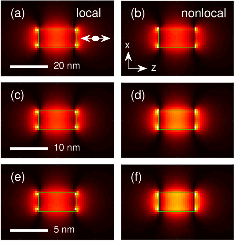
Figure 1: Comparison between the local QNM (a,c,e), $\left|\mathbf{\tilde{f}}(x,z,y_{0})\right|^{2}$, and the nonlocal GNOR QNM (b,d,f), $\left|\mathbf{\tilde{f}}^{{\rm nl}}(x,z,y_{0})\right|^{2}$ for nanorods of different heights, $h=20\,{\rm nm}$, $h=10\,{\rm nm}$ and $h=5\,{\rm nm}$, where $y_{0}=0$ is at the center of the nanorods. The same geometrical aspect ratio of 2 is used corresponding to a radius of $r=5\,{\rm nm}$ for the largest resonator. The double arrow in (a) shows the location of the dipole emitter at $10\,{\rm nm}$ away from the metallic surface, that is kept the same for all QNM calculations, and the green box represents the metallic border.

Depicted in Fig. 1 are the computed QNMs for three different gold cylindrical nanorods with the same aspect ratio, varying from $20\,{\rm nm}$ to $5\,{\rm nm}$ in length (see figure caption for details). The left panels represent the local Drude model QNMs while the right panels show the QNMs using the nonlocal GNOR model. As seen, the main QNM shapes are similar but a redistribution of the localized field clearly occurs due to the inclusion of the nonlocal corrections. While the local Drude model predicts a similar mode shape for the different nanoparticle sizes, the nonlocal corrections introduce a pronounced degree of modal reshaping for smaller nanoparticles. Indeed, even for the largest nanoparticle shown in Figs. 1(a,b), higher field values are seen both inside as well as outside (but near) the metallic region.

III.2 Purcell factors from coupled dipole emitters

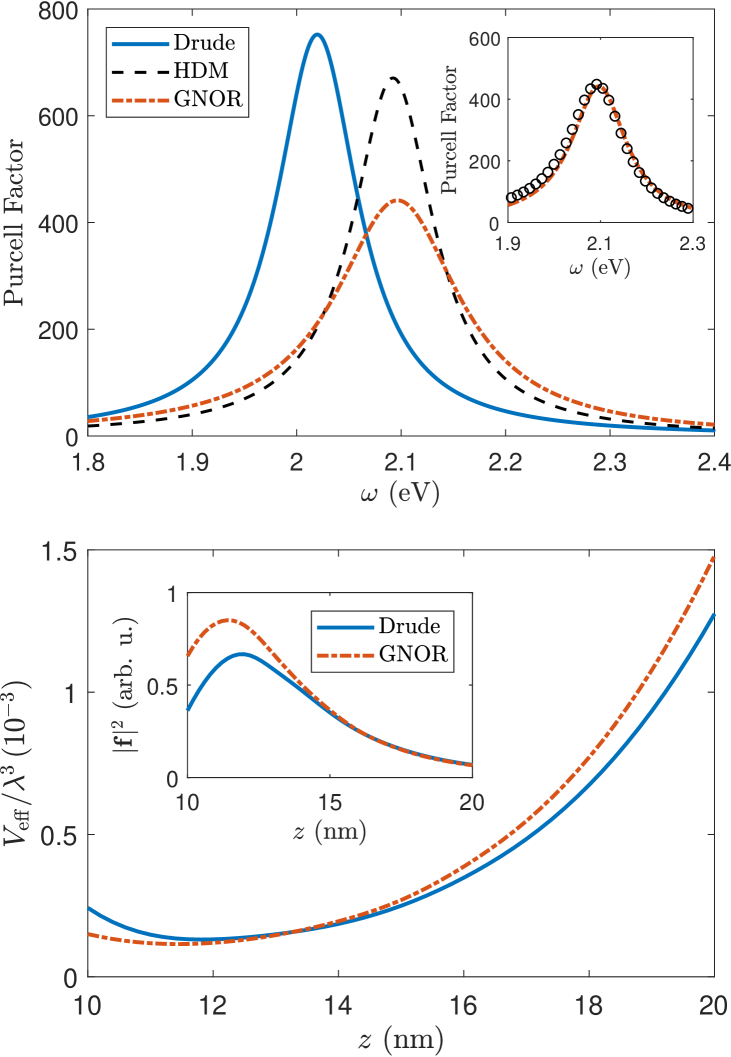
Figure 2: Top: Generalized Purcell factor for a dipole emitter placed $10\,{\rm nm}$ away form a gold nanorod of height $h=20\,{\rm nm}$ and radius of $r=5\,{\rm nm}$, using Drude QNM, nonlocal HDM QNM and nonlocal GNOR QNM. The inset shows the agreement between full dipole calculations (with no approximations) and GNOR QNM results. Bottom: The corresponding QNM effective mode volume, ${\rm V}_{{\rm eff}}$, is shown for a range of locations above the nanorod. Note that $z=10\,{\rm nm}$ is at the surface of the metallic nanoparticle. The inset shows the modal absolute magnitude for completeness.

Figure 2 shows the computed QNM Purcell factors using the local Drude model as well as the two different nonlocal models for the $h=20\,{\rm nm}$ nanorod. As can be seen, both HDM and GNOR models predict the known blueshift of the plasmonic resonance McMahon et al. (2009); Raza et al. (2011); Teperik et al. (2013). However, the nonlocal prediction of the peak enhancement strongly depends on the model chosen. The GNOR model in particular predicts a considerably lower Purcell factor due to the inclusion of diffusion, which accounts for surface-enhanced Landau damping Mortensen et al. (2014). Indeed, as will be discussed shortly, including the nonlocal effects modifies both the quality factor and the mode volume associated with QNMs. The inset also shows the validity of our Purcell factor calculations against full-dipole numerical calculations, only shown for the nonlocal GNOR response. However, a similar degree of agreement is observed for all other calculations both in Fig. 2 and what follows.

In Fig. 2, bottom panel, we additionally plot the corresponding effective mode volume for a range of dipole locations, from the nanorod surface (at $z=10$ nm) up to $10\,{\rm nm}$ away. A comparison between the local Drude model (solid-blue) and the nonlocal GNOR (dashed-red) is shown where a nontrivial difference is observed. Closer to the metallic surface, smaller effective mode volumes are predicted by the nonlocal corrections while further away the opposite takes place. The difference at larger distances however, is mainly due to nonlocal corrected resonant wavelengths that are used to normalize the mode volumes.

We also consider enhanced SE from the three different gold nanoparticles discussed in Fig. 1. Plotted in Fig. 3 are the QNM calculations of the Purcell factors for dipole emitters located $10\,{\rm nm}$ away from nanorods, on the $z$-axis. In each case, the local Drude results are compared with the nonlocal GNOR results. Clearly, nonlocal corrections result in both larger resonance blueshifts and larger damping rates (lower quality factors).

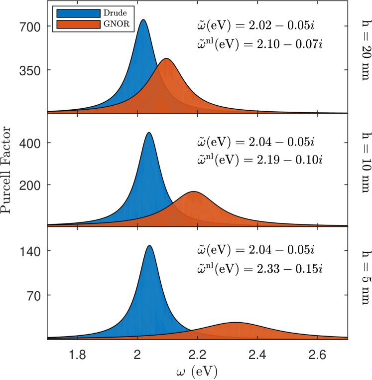
Figure 3: Size-dependent discrepancy in Purcell factor between the local Drude model and the nonlocal GNOR model. Results are derived form analytical QNM calculations when the dipole emitter is kept $10\,{\rm nm}$ away along the z-axis. The complex resonance frequencies for both models are also shown in each case.

III.3 Computing EELS spatial maps

For our next application of the nonlocal QNM theory, we calculate the spatial maps associated with EELS experiments that are obtained by nanometer-scale resolution in microscopy of LSP resonances Rossouw et al. (2011); Nicoletti et al. (2011); Husnik et al. (2013); Hobbs et al. (2016); Shekhar et al. (2017). Since the GF is available at all locations through QNM expansion of (5), the EELS spectra in the $xz$ plane subjected to an electron beam propagating along the $y$ axis can be easily obtained from Rossouw et al. (2011); Ge and Hughes (2016),

$$\Gamma\left(x,z;\omega\right)=$$ (9)

$$\quad-\frac{4e^{2}v^{2}}{\hbar}\int dtdt^{\prime}{\rm Im}\left\{e^{i\omega\left(t^{\prime}-t\right)}G_{yy}\left(\mathbf{r}_{e}\left(t\right),\mathbf{r}_{e}\left(t^{\prime}\right);\omega\right)\right\},$$

where $v$ is the speed of electrons, and the single mode expansion for our Green function—that is already confirmed to be very accurate—is used. The EELS calculations for all three nanoparticles (of Fig. 1) are shown in Fig. 4, all computed at the corresponding plasmonic peaks frequencies. Note that there are some noticeable numerical problems around the sharp corners of the metallic nanorod when using the conventional Drude model theory on the left (which is a known problem Sukhorukov et al. (2006); Wallén et al. (2008)). Using the same meshing scheme, however, the nonlocal description evidently helps to avoid such nonphysical predictions. More importantly, as the nanoparticle size decreases the EELS map becomes brighter at its maximum location which originates from the higher modal amplitudes of the QNMs discussed in Fig. 1. We stress that with the computed QNMs, such EELS maps are calculated instantaneously, which is a far cry from the usual brute force numerical solvers.

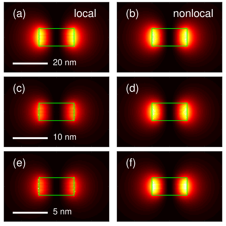
Figure 4: Comparison between the EELS map of the plasmonic nanorod using the local Drude model, (a,c,e), and the nonlocal GNOR model, (b,d,f), where each map is calculated at the corresponding plasmonic peak frequency. Same geometries as in Fig. 1 are used and the green box represents the metallic border.

III.4 Field-driven Mollow triplets and quantum optics regime

Finally, in addition to the previous discussions on Purcell factor and mode volume that are essential for building quantum optical models of light-matter interaction Bozhevolnyi and Khurgin (2017), we discuss the quantum regime of field-driven Mollow triplets for QDs coupled to plasmonic nanoparticles. In the dipole and rotating wave approximations, the total Hamiltonian of the coupled system can be written as Scheel et al. (1999); Ge et al. (2013)

$$H=\hbar\int d{\bf r}\int_{0}^{\infty}d\omega\,\omega\,{\bf\hat{f}}^{\dagger}({\bf r},\omega){\bf\hat{f}}({\bf r},\omega)+\hbar\omega_{x}\sigma^{+}\sigma^{-}$$ (10)

$$-\left[\sigma^{+}\int_{0}^{\infty}\!d\omega\,{\bf d}\cdot{\bf\hat{E}}({\bf r}_{d},\omega)+{\rm H.c.}\right]+\frac{\hbar\Omega}{2}\left(\sigma^{+}e^{-i\omega_{L}}+\sigma^{-}e^{i\omega_{L}}\right),$$

where $\Omega=\braket{{\bf\hat{E}}_{\rm pump}({\bf r}_{d})}\cdot{\bf d}/\hbar$ is the effective Rabi field, $\sigma^{+},\sigma^{-}$ are the Pauli operators of the two-level atom (or exciton), $\omega_{x}$ is the resonance of the exciton, ${\bf d}$ is the dipole of the exciton, and ${\bf\hat{f}},{\bf\hat{f}}^{\dagger}$ are the boson field operators. Following the approach in Ref. Ge et al. (2013), and using the interaction picture at the laser frequency $\omega_{L}$, one can derive a self-consistent generalized master equation in the 2nd-order Born-Markov approximation:

$$\frac{\partial{\rho}}{\partial t} =\frac{1}{i\hbar}[H_{S},\rho]+\int_{0}^{t}d\tau\left\{{\tilde{J}_{\rm ph}(\tau)}[-\sigma^{+}\sigma^{-}(-\tau)\rho\,+\right.$$

$$\left.\phantom{\tilde{J}_{\rm ph}}+\sigma^{-}(-\tau)\rho\sigma^{+}]+{\rm H.c.}\right\},$$ (11)

where $\tilde{J}_{\rm ph}(\tau)=\int_{0}^{\infty}d\omega J_{\rm ph}(\omega)e^{i(\omega_{L}-\omega)\tau}$, with the photon-reservoir spectral function given by $J_{\rm ph}(\omega)\equiv\frac{{\bf d}\cdot{\rm Im}[{\bf G}({\bf r}_{d},{\bf r}_{d};\omega)]{\bf\cdot d}}{\pi\hbar\varepsilon_{0}}$, and the time-dependent operators are defined through $\sigma^{\pm}(-\tau)=e^{-iH_{S}\tau/\hbar}\sigma^{\pm}e^{iH_{S}\tau/\hbar}$, with $H_{S}=\hbar(\omega_{x}-\omega_{L})\sigma^{+}\sigma^{-}+\hbar\Omega/2(\sigma^{+}+\sigma^{-})$, which results in a complex interplay between the values of the local density of states at the field-driven dressed states. Solving the master equation, and exploiting the quantum regression theorem, one can compute the incoherent spectrum of the QD emission from Ge et al. (2013)

$$S_{0}\left(\omega\right) =\lim_{t\rightarrow\infty}\textrm{Re}\left[\int_{0}^{\infty}d\tau\left(\left\langle\sigma^{+}(t-\tau)\sigma^{-}(t)\right\rangle\right.\right.$$ (12)

$$-\left.\left.\left\langle\sigma^{+}(t)\rangle\langle\sigma^{-}(t)\right\rangle\right)e^{i(\omega_{L}-\omega)\tau}\right],$$

as well as the detected spectrum, which includes quenching and propagation from QD at $\mathbf{r}_{0}$ to a point detector at $\mathbf{r}_{D}$, from Ge et al. (2013)

$$S\left(\mathbf{r}_{D};\omega\right)=\frac{2}{\varepsilon_{0}}\,|\mathbf{G}(\mathbf{r}_{D},\mathbf{r}_{0};\omega)\cdot\mathbf{d}|^{2}\,S_{0}(\omega).$$ (13)

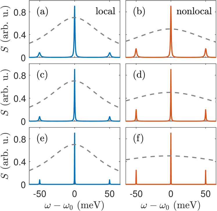
Figure 5: Detected spectra ($S$ evaluated at ${\bf r}_{D}=200\,\textrm{nm}$) of a field-driven QD coupled to plasmonic nanoparticles, where the same ordering of the particle size and QD location as in Fig. 1 is followed, and we use an effective Rabi field of $\Omega=50\,\mbox{meV}$. The plasmonic enhancement is also shown in dashed-gray in background. Nonlocal investigations on the right predict relatively stronger side peaks for the Mollow triplet with narrower linewidths.

For example calculations, we assume a QD with the dipole moment of $|\mathbf{d}|=50\,\mbox{Debye}$ at $10\,\textrm{nm}$ away from the nanoparticle surface, at $x$=$0$. In particular, as with the calculations above, we compare the local Drude model versus nonlocal GNOR model as shown in Fig. 5. As can be recognized, including the nonlocal effects, in general, predicts narrower linewidths for the Mollow triplets (see e.g. Table 1) where the relative strength of the side peaks are also increased. This is attributed to the modified plasmonic enhancment in the nonlocal description as confirmed in Fig. 3, which can be also rigorously confirmed using analytical equations for the linewdiths derived in Ge et al. (2013). It should be noted that, in general, the detected spectrum $S$ for the Mollow triplet problem can be different than the emitted $S_{0}$ as discussed in Ge et al. (2013), however in our particular case, under the resonant excitation, we find that they have the same qualitative shape (and differ only quantitatively). We also stress that, these spectral calculations, at any detector position, can be trivially performed using a standard desktop through use of semi-analytical GF of (5), demonstrating the power of our approach for carrying out complex problems in quantum optics.

$h$ (nm)	Drude FWHM (meV)	GNOR FWHM (meV)
20	1.28	1.21
10	0.74	0.61
5	0.45	0.42

Table 1: Linewidth of the central Mollow peak for the three nanoparticles, using both Drude model and GNOR model. Same trend holds for the side peaks.

IV Conclusions

We have presented an efficient and accurate modal description of the nonlocal response of arbitrarily shaped metallic nanoparticles, using a fully 3D model. We have shown how analytical nonlocal QNMs can be used to accurately construct the system GF from which modal quantities of interest such as Purcell factor and effective mode volume can be derived. As anticipated, we first observe the blueshift as well as the larger damping rate for the LSP as a consequence of nonlocal effects. We further confirmed the validity of our approach for different nanoparticle sizes with full dipole solutions of the modified Maxwell equations, and we were able to successfully predict the size-dependent nonlocal modifications with ease. As example applications of the theory, we described how our nonlocal QNMs can be used to efficiently model Purcell factors of dipole emitters, EELS spatial maps as well as Mollow triplet spectra of field-driven QD. The presented model has many applications in both classical and quantum nanoplasmonics, offers considerable analytical insight into complex nonlocal problems, and could help pave the way for a quantum description of both light and matter.

Funding Information

We acknowledge funding from Queen’s University, the Natural Sciences and Engineering Research Council of Canada, the People Programme (Marie Curie Actions) of the European Union’s Seventh Framework Programme (FP7/2007-2013) under REA grant agreement number 609405 (COFUNDPostdocDTU), Villum Fonden (VILLUM Investigator grant no. 16498) and the Danish National Research Council (DNRF103).

References

- Ciracì et al. (2012) C. Ciracì, R. T. Hill, J. J. Mock, Y. Urzhumov, A. I. Fernández-Domínguez, S. A. Maier, J. B. Pendry, A. Chilkoti, and D. R. Smith, Science 337, 1072 (2012).
- Savage et al. (2012) K. J. Savage, M. M. Hawkeye, R. Esteban, A. G. Borisov, J. Aizpurua, and J. J. Baumberg, Nature 491, 574 (2012).
- Esteban et al. (2012) R. Esteban, A. G. Borisov, P. Nordlander, and J. Aizpurua, Nat. Commun. 3, 825 (2012).
- Pelton (2015) M. Pelton, Nat Photon 9, 427 (2015).
- Barbry et al. (2015) M. Barbry, P. Koval, F. Marchesin, R. Esteban, A. G. Borisov, J. Aizpurua, and D. Sánchez-Portal, Nano Lett. 15, 3410 (2015).
- Hoang et al. (2016) T. B. Hoang, G. M. Akselrod, and M. H. Mikkelsen, Nano Lett. 16, 270 (2016).
- Bozhevolnyi and Mortensen (2017) S. I. Bozhevolnyi and N. A. Mortensen, Nanophotonics 6, 1185 (2017).
- Ruppin (1973) R. Ruppin, Phys. Rev. Lett. 31, 1434 (1973).
- Fuchs and Claro (1987) R. Fuchs and F. Claro, Phys. Rev. B 35, 3722 (1987).
- Leung (1990) P. T. Leung, Phys. Rev. B 42, 7622 (1990).
- García de Abajo (2008) F. J. García de Abajo, J. Phys. Chem. C 112, 17983 (2008).
- McMahon et al. (2009) J. M. McMahon, S. K. Gray, and G. C. Schatz, Phys. Rev. Lett. 103, 097405 (2009).
- Raza et al. (2011) S. Raza, G. Toscano, A.-P. Jauho, M. Wubs, and N. A. Mortensen, Phys. Rev. B 84, 121412 (2011).
- Teperik et al. (2013) T. V. Teperik, P. Nordlander, J. Aizpurua, and A. G. Borisov, Phys. Rev. Lett. 110, 1 (2013).
- Mortensen et al. (2014) N. A. Mortensen, S. Raza, M. Wubs, T. Søndergaard, and S. I. Bozhevolnyi, Nat. Commun. 5, 1 (2014).
- Wiener et al. (2012) A. Wiener, A. I. Fernández-Domínguez, A. P. Horsfield, J. B. Pendry, and S. A. Maier, Nano Lett. 12, 3308 (2012).
- Stella et al. (2013) L. Stella, P. Zhang, F. J. GarciÂa-Vidal, A. Rubio, and P. GarciÂa-Gonzalez, The Journal of Physical Chemistry C 117, 8941 (2013).
- Filter et al. (2014) R. Filter, C. Bösel, G. Toscano, F. Lederer, and C. Rockstuhl, Opt. Lett. 39, 6118 (2014).
- Kristensen and Hughes (2014) P. T. Kristensen and S. Hughes, ACS Photonics 1, 2 (2014).
- Kamandar Dezfouli et al. (2017) M. Kamandar Dezfouli, R. Gordon, and S. Hughes, Phys. Rev. A 95, 013846 (2017).
- Leung et al. (1994) P. T. Leung, S. Y. Liu, S. S. Tong, and K. Young, Phys. Rev. A 49, 3068 (1994).
- Kristensen et al. (2012) P. T. Kristensen, C. P. Van Vlack, and S. Hughes, Opt. Lett. 37, 1649 (2012).
- Sauvan et al. (2013) C. Sauvan, J. P. Hugonin, I. S. Maksymov, and P. Lalanne, Phys. Rev. Lett. 110, 237401 (2013).
- Kristensen et al. (2015) P. T. Kristensen, R. C. Ge, and S. Hughes, Phys. Rev. A 92, 053810 (2015).
- Bai et al. (2013) Q. Bai, M. Perrin, C. Sauvan, J.-P. Hugonin, and P. Lalanne, Opt. Exp. 21, 27371 (2013).
- Muljarov and Langbein (2016) E. A. Muljarov and W. Langbein, Phys. Rev. B 94, 235438 (2016).
- Purcell et al. (1946) E. M. Purcell, H. C. Torrey, and R. V. Pound, Phys. Rev. 69, 37 (1946).
- Ford and Weber (1984) G. Ford and W. Weber, Physics Reports 113, 195 (1984).
- Sipe (1987) J. E. Sipe, J. Opt. Soc. Am. B 4, 481 (1987).
- Agarwal (2000) G. S. Agarwal, Phys. Rev. Lett. 84, 5500 (2000).
- Wubs et al. (2004) M. Wubs, L. G. Suttorp, and A. Lagendijk, Phys. Rev. A 70, 053823 (2004).
- Anger et al. (2006) P. Anger, P. Bharadwaj, and L. Novotny, Phys. Rev. Lett. 96, 3 (2006).
- Hughes and Kamada (2004) S. Hughes and H. Kamada, Phys. Rev. B 70, 195313 (2004).
- Manga Rao and Hughes (2007) V. S. C. Manga Rao and S. Hughes, Phys. Rev. Lett. 99, 193901 (2007).
- Van Vlack et al. (2012) C. Van Vlack, P. T. Kristensen, and S. Hughes, Phys. Rev. B 85, 075303 (2012).
- Yan et al. (2013) W. Yan, N. A. Mortensen, and M. Wubs, Phys. Rev. B 88, 155414 (2013).
- Ge et al. (2014) R. C. Ge, P. T. Kristensen, J. F. Young, and S. Hughes, New J. Phys. 16, 113048 (2014).
- Kamandar Dezfouli and Hughes (2017) M. Kamandar Dezfouli and S. Hughes, ACS Photonics 4, 1245 (2017).
- García De Abajo and Kociak (2008) F. J. García De Abajo and M. Kociak, Phys. Rev. Lett. 100, 106804 (2008).
- Rossouw et al. (2011) D. Rossouw, M. Couillard, J. Vickery, E. Kumacheva, and G. A. Botton, Nano Lett. 11, 1499 (2011).
- Nicoletti et al. (2011) O. Nicoletti, M. Wubs, N. A. Mortensen, W. Sigle, P. A. van Aken, and P. A. Midgley, Opt. Exp. 19, 15371 (2011).
- Mohammadi et al. (2012) Z. Mohammadi, C. P. Van Vlack, S. Hughes, J. Bornemann, and R. Gordon, Opt. Exp. 20, 15024 (2012).
- Boudarham and Kociak (2012) G. Boudarham and M. Kociak, Phys. Rev. B 85, 245447 (2012).
- Husnik et al. (2013) M. Husnik, F. Von Cube, S. Irsen, S. Linden, J. Niegemann, K. Busch, and M. Wegener, Nanophotonics 2, 241 (2013).
- Christensen et al. (2014) T. Christensen, W. Yan, S. Raza, A. P. Jauho, N. A. Mortensen, and M. Wubs, ACS Nano 8, 1745 (2014).
- Raza et al. (2015) S. Raza, S. Kadkhodazadeh, T. Christensen, M. Di Vece, M. Wubs, N. A. Mortensen, and N. Stenger, Nat. Commun. 6, 8788 (2015).
- Hörl et al. (2015) A. Hörl, A. Trügler, and U. Hohenester, ACS Photonics 2, 1429 (2015).
- Ge and Hughes (2016) R.-C. Ge and S. Hughes, J. Opt. 18, 054002 (2016).
- Hobbs et al. (2016) R. G. Hobbs, V. R. Manfrinato, Y. Yang, S. A. Goodman, L. Zhang, E. A. Stach, and K. K. Berggren, Nano Lett. 16, 4149 (2016).
- Shekhar et al. (2017) P. Shekhar, M. Malac, V. Gaind, N. Dalili, A. Meldrum, and Z. Jacob, ACS Photonics 4, 1009 (2017).
- Aharonovich et al. (2016) I. Aharonovich, D. Englund, and M. Toth, Nat. Photon. 10, 631 (2016).
- Ge et al. (2013) R.-C. Ge, C. Van Vlack, P. Yao, J. F. Young, and S. Hughes, Phys. Rev. B 87, 205425 (2013).
- Ge and Hughes (2014) R.-C. Ge and S. Hughes, Opt. Lett. 39, 4235 (2014).
- McMahon et al. (2010) J. M. McMahon, S. K. Gray, and G. C. Schatz, Phys. Rev. B 82, 035423 (2010).
- Tserkezis et al. (2016a) C. Tserkezis, J. R. Maack, Z. Liu, M. Wubs, and N. A. Mortensen, Sci. Rep. 6, 28441 (2016a).
- Axelrod et al. (2017) S. Axelrod, M. Kamandar Dezfouli, H. M. K. Wong, A. S. Helmy, and S. Hughes, Phys. Rev. B 95, 155424 (2017).
- Toscano et al. (2012) G. Toscano, S. Raza, A.-P. Jauho, N. A. Mortensen, and M. Wubs, Opt. Exp. 20, 4176 (2012).
- Tserkezis et al. (2016b) C. Tserkezis, N. Stefanou, M. Wubs, and N. A. Mortensen, Nanoscale 8, 17532 (2016b).
- (59) COMSOL Multiphysics: www.comsol.com.
- Sukhorukov et al. (2006) A. A. Sukhorukov, I. V. Shadrivov, and Y. S. Kivshar, International Journal of Numerical Modelling: Electronic Networks, Devices and Fields 19, 105 (2006).
- Wallén et al. (2008) H. Wallén, H. Kettunen, and A. Sihvola, Metamaterials 2, 113 (2008).
- Bozhevolnyi and Khurgin (2017) S. I. Bozhevolnyi and J. B. Khurgin, Nat. Photon. 11, 398 (2017).
- Scheel et al. (1999) S. Scheel, L. Knöll, and D.-G. Welsch, Phys. Rev. A 60, 4094 (1999).