Solitary potentials in a three component space plasma

Abstract

The heavy ion acoustic solitary waves (HIASWs) in a magnetized, collisionless, three component space plasma system in the presence of dynamical heavy particles and bi-kappa distributed two distinct temperature of electrons has been carried out. The Korteweg-de Vries (K-dV), the modified K-dV (mK-dV), and the further mK-dV (fmK-dV) equations are derived by employing the well known reductive perturbation method. The basic features of HIASWs (speed, amplitude, width etc.) are found to be significantly modified by the effects of number density of plasma species, superthermal electrons with two distinct temperatures and the magnetic field (obliqueness). The K-dV and fm-KdV solitons exhibit both compressive and rarefactive structures, whereas the mK-dV solitons support only compressive structures. In order to trace the vicinity of the critical heavy ion density, neither the magnetized KdV nor magnetized mKdV equation is suitable for describing the HIASWs. Therefore, we have considered a higher order nonlinearity to describe the solitary profiles by deriving fmK-dV equation. The implication of our results in some space and laboratory plasma situations are concisely discussed.

I Introduction

Recently, propagation of linear and nonlinear waves in electron-ion (EI) plasma has generated a lot of interest among the researchers Chen1984 ; Durrani1979 ; Davidson1972 ; Chawla2013 ; Mamun1997 . Since many nonlinear fascinating structures like solitary waves, solitons, shocks, double layers and so on are observed in space, astrophysical, and laboratory plasmas, so a large number of investigations are going on it Hossen2014a ; Hossen2014b ; Hossen2014c ; Hossen2014d ; Hosen2016 . The existence of ions in astrophysical plasmas has been affirmed experimentally by detecting of a noble gas molecular ion in the crab nebula Barlow2013 . EI plasmas exists in Milky way galaxy Burns1983 , polar region of neutron stars Michel1991 , active galactic nuclei Miller1987 , pulsar magnetosphere Goldreich1969 and the early universe Rees1983 etc. Ion acoustic waves play a vital role to study the nonlinear features of localized electrostatic disturbances in laboratory plasmas Lonngren1983 ; Nakamura1985 ; Koga1993 as well as in space plasmas Witt1983 ; Qian1988 ; Marchenko1995 .

Generally, the particle distribution near equilibrium in a plasma system is often considered to be Maxwellian, for modeling purposes. But from the space plasma observations, it has been proven that the presence of the ion and electron populations as astrophysical plasma contexts are far off from their thermal equilibrium state. Due to the effect of external forces or to wave particle interaction in numerous space plasma observations Vocks2003 ; Gloeckler2006 and laboratory experiments Yagi1997 ; Preische1996 indicate the appearance of highly energetic (superthermal) particles. The existence of accelerated, energetic (superthermal) particles in the measurement of electron distribution in near-Earth space environments suggest a (often strong) deviation from Maxwellian equilibrium Maksimovic1997 ; Gloeckler2006 ; Chaston1997 . So Maxwellian Boltzmann distribution is possibly imperfect for explicating the interaction of superthermal particles. However, the plasma system containing higher energetic (Superthermal) particle with energies greater than the energies of the particles exist in thermal equilibrium can be fitted more appropriately via the $\kappa$ (kappa) type of Lorentzian distribution function (df) Vasyliunas1968 ; Summers1991 ; Hellberg2009 than via the thermal Maxwellian df where the real parameter $\kappa$ measures the deviation from a Maxwellian distribution (the smaller the value, the larger the deviation from a Maxwellian, in fact attained for infinite $\kappa$). Hence we focus on a plasma system with superthermal particles modelled by a $\kappa$- distribution Hellberg2009 .

The isotropic three-dimensional (3D) kappa velocity distribution of particles of mass m is of the form

$$F_{k}(v)=\frac{\Gamma(k+1)}{(\pi k\omega)^{(3/2)}\Gamma(k-1/2)}(1+\frac{v^{2}}{k\omega^{2}})^{-(k+1)},$$ (1)

where, $F_{k}$ symbolizes the kappa distribution function, $\Gamma$ is the gamma function, $\omega$ shows the most probable speed of the energetic particles, given by $\omega=[(2k-3/k)^{1/2}(k_{B}T/m)^{1/2}]$, with $T$ being the characteristic kinetic temperature and $\omega$ is related to the thermal speed $V_{t}=(k_{B}T/m)^{1/2}$ and, the parameter $k$ represents the spectral index Cattaert2007 which defines the strength of the superthermality. The range of this parameter is $3/2<k<\infty$ Alam2013 . In the limit $k\rightarrow\infty$ Basu2008 ; Baluku2012 the kappa distribution function reduces to the well-known Maxwellian Boltzmann distribution.

Recently, a numerous investigations have been made by many authors on ion-acoustic solitary waves (IASWs) with single-temperature superthermal (kappa distributed) electrons Hussain2012 ; Shahmansouri2013 ; Sultana2011 . Schippers et al. Schippers2008 have combined a hot and a cold electron component, while both electrons are kappa distributed and found a best fit for the electron velocity distribution. Baluku et al. Baluku2011 used this model as base of a kinetic theory study for electron-acoustic waves in Saturn s magnetosphere and then they have studied IA solitons in a plasma with two-temperature kappa distributed electrons. Pakzad Pakzad2011 studied a dissipative plasma system with superthermal electrons and positrons and, found the effects of ion kinematic viscosity and the superthermal parameter on the IA waves. Tasnim et al. Tasnim2013a ; Tasnim2013b also considered two-temperature nonthermal ions and discussed the properties of shock waves. Masud et al. Masud2013 have studied the characteristic of DIA shock waves in an unmagnetized dusty plasma consisting of negatively charged static dust, inertial ions, positively charged positrons following Maxwellian distribution, and superthermal electrons with two distinct temperatures. Lu et al. Lu2005 studied the EA solitary structures with positive charged potentials in a three-component plasma system containing cold, hot, and beam electrons. By using the small-k expansion perturbation method, the three-dimensional stability of dust-ion acoustic solitary waves in a magnetized multicomponent dusty plasma containing negative heavy ions and stationary variable-charge dust particles was analyzed by El-Taibany et al. El-Taibany2011 . Shahmansouri Shahmansouri2012 investigated the basic properties of IA waves in an unmagnetized plasma including cool ions and hot ions with kappa distributed electrons using small amplitude techniques and observed that the suprathermality effects play a pivotal role as the properties of IA solitons significantly affect through the ion and the electron superthermal index. Since, dynamical heavy particles and higher order nonlinearity play a vital role to describe the different nonlinear structures of astrophysical objects. Therefore, our main intention to carry the higher order nonlinearity by deriving extention of mK-dV equation, namely further mK-dV (fmK-dV) and also considering the dynamics of heavy particles to describe HIASWs in such plasma system under consideration. Recently, Ema et al. Ema2015a ; Ema2015b studied the effect of adiabacity on the heavy ion acoustic (HIA) solitary and shock waves in a strongly coupled nonextensive plasma. They observed that the roles of the adiabatic positively charged heavy ions, and nonextensivity of electrons have significantly modified the basic features (viz., polarity, amplitude, width, etc.) of the HIA solitary/shock waves. Hossen et al. Hossen2014m ; Hossen2014n ; Hossen2015o considered positively charged static heavy ions in a relativistic degenerate plasma and rigorously investigated the basic features of solitary and shock structures. By considering superthermal electrons and adiabatic heavy ions Shah et al. Shah2015a ; Shah2016 investigated the basic features of HIA solitary and shock waves by considering both planar and nonplanar geometry.

Up to the best of our knowledge, no theoretical investigations have been worked out to study of HIASWs with two temperature superthermal (kappa distributed) electrons in EI plasma. Therefore, in our present work, we attempt to study the basic features of HIA waves by deriving the magnetized Korteweg-de Vries (K-dV) and magnetized modified K-dV (mK-dV) equations in EI plasma containing superthermal electrons and Heavy ion.

II Theoretical model and basic equations

We consider a three component magnetized plasma system containing positively charged heavy ions and kappa distributed electrons with two distinct temperatures. Therefore, at equilibrium condition, $n_{hi0}=n_{ce0}+n_{he0}$, where $n_{hi0}$ is the unperturbed heavy ion number density, $n_{ce0}$ and $n_{he0}$ are the density of unperturbed lower and higher temperature electron respectively. The dynamics of the heavy ion acoustic waves are described by the following (normalized) equations:

$$\frac{\partial n_{h}}{\partial t}+\nabla.({n_{h}}{\textbf{u}_{h}})=0,$$ (2)

$$\frac{\partial\textbf{u}_{h}}{\partial t}+({\textbf{u}_{h}}.\nabla)u_{h}=-\nabla\phi+\alpha({\textbf{u}_{h}}\times{\hat{z}}).$$ (3)

The Poisson s equation can be written as

$$\nabla^{2}\phi=\mu_{ce}\left(1-\frac{\sigma_{1}\phi}{k_{ce}-\frac{3}{2}}\right)^{-k_{ce}+\frac{1}{2}}-n_{h}$$

$$+\mu_{he}\left(1-\frac{\sigma_{2}\phi}{k_{he}-\frac{3}{2}}\right)^{-k_{he}+\frac{1}{2}},$$ (4)

where, $n_{h}$ is the heavy ion particle number density normalized by its equilibrium value $n_{hi0}$, $\textbf{u}_{h}$ is the heavy ion fluid speed normalized by $C_{h}=(k_{B}T_{ef}/m_{h})^{1/2}$, $\phi$ is the electrostatic wave potential normalized by $k_{B}T_{ef}/e,\sigma_{1}=T_{ef}/T_{ce},\sigma_{2}=T_{ef}/T_{he},\mu_{ce}=n_{ce0}/n_{hi0},\mu_{he}=n_{he0}/n_{hi0},\alpha=\omega_{hc}/\omega_{ph}$, where $T_{ef}=n_{e0}T_{ce}T_{he}/(n_{ce0}T_{he}+n_{he0}T_{ce})$. It should be noted that $n_{e0}$ is the total electron number density at equilibrium and $T_{ce}(T_{he})$ is the lower (higher) electron temperature, $T_{ef}$ is the effective temperature of two electrons, $k_{ce}$ and $k_{he}$ are spectral index, $\omega_{hc}$ is the heavy ion cyclotron frequency, $\omega_{p}$ is the plasma frequency, $k_{B}$ is the Boltzmann constant and e is the magnitude of the electron charge. The time variable ($t$) is normalized by ${\omega_{ph}}=(4\pi n_{hi0}e^{2}/m_{h})^{1/2}$, and the space variable ($x$) is normalized by $\lambda_{h}=(m_{e}c^{2}/4\pi n_{hi0}e^{2})^{1/2}$.

III Nonlinear Equations

III.1 Derivation of the Magnetized K-dV Equation

At first we use reductive perturbation method to derive the well known K-dV equation. We apply the reductive perturbation technique in which independent variables are stretched as

$$\xi=\epsilon^{1/2}(L_{x}\hat{x}+L_{y}\hat{y}+L_{z}\hat{z}-V_{p}t),$$ (5)

$$\tau={\epsilon}^{3/2}t,$$ (6)

where, $V_{p}$ is the phase velocity of HIA wave and $\epsilon$ is a smallness parameter measuring the weakness of the dispersion $(0<\epsilon<1)$ and $L_{x}$, $L_{y}$, and $L_{z}$ are the directional cosines of the wave vector k along the x, y, and z axes respectively, so that $L_{x}^{2}+L_{y}^{2}+L_{z}^{2}=1$. For a dynamical equation, we also expand the perturbed quantities $n_{h}$, $u_{h}$ and $\phi$ in power series of $\epsilon$. We may expand $n_{h}$, $u_{h}$, and $\phi$ in power series of $\epsilon$ as

$$n_{h}=1+\epsilon n_{h}^{(1)}+\epsilon^{2}n_{h}^{(2)}+\cdot\cdot\cdot,$$ (7)

$$u_{hx,y}=0+\epsilon^{3/2}u_{hx,y}^{(1)}+\epsilon^{2}u_{hx,y}^{(2)}+\cdot\cdot\cdot,$$ (8)

$$u_{hz}=0+\epsilon u_{hz}^{(1)}+\epsilon^{2}u_{hz}^{(2)}+\cdot\cdot\cdot,$$ (9)

$$\phi=0+\epsilon\phi^{(1)}+\epsilon^{2}\phi^{(2)}+\cdot\cdot\cdot.$$ (10)

Now, applying Eqs. (5)-(10) into Eqs. (2) - (4) and taking the lowest order coefficient of $\epsilon$, we obtain, $u_{hz}^{(1)}={L_{z}\phi^{(1)}}/{V_{p}}$, $n_{h}^{(1)}={L_{z}^{2}\phi^{(1)}}/{V_{p}^{2}}$ and $V_{p}=L_{z}/\sqrt{\mu_{ce}c_{1}+\mu_{he}d_{1}}$ represents the dispersion relation for the HIA waves that move along the propagation vector $k$. To the next higher order of $\epsilon$, we obtain a set of equations after using the value of $u_{hz}^{(1)}$, $n_{hz}^{(1)}$, $V_{p}$ and taking the z-component of momentum equation as

$$\frac{\partial n_{h}^{(1)}}{\partial\tau}-v_{p}\frac{\partial n_{h}^{(2)}}{\partial\xi}+L_{x}\frac{\partial u_{hx}^{(2)}}{\partial\xi}$$

$$+L_{y}\frac{\partial u_{hy}^{(2)}}{\partial\xi}+L_{z}\frac{\partial u_{hz}^{(2)}}{\partial\xi}+L_{z}\frac{\partial{(n_{h}^{(1)}u_{hz}^{(1)})}}{\partial\xi}=0,$$ (11)

$$\frac{\partial u_{hz}^{(1)}}{\partial\tau}-v_{p}\frac{\partial u_{hz}^{(2)}}{\partial\xi}+L_{z}u_{hz}^{(1)}\frac{\partial u_{hz}^{(1)}}{\partial\xi}+L_{z}\frac{\partial{\phi^{(2)}}}{\partial\xi}=0,$$ (12)

$$\frac{\partial^{2}\phi^{(1)}}{\partial\xi^{2}}=\mu_{ce}c_{1}\phi^{(2)}+\mu_{ce}c_{2}\phi{{}^{(1)}}^{2}$$

$$-n_{h}^{(2)}+\mu_{he}d_{1}\phi^{(2)}+\mu_{he}d_{2}\phi{{}^{(1)}}^{2}.\$$ (13)

Again taking the co-efficient of $\epsilon^{2}$ for x-and y- component from momentum equation we get

$$u_{hy}^{(2)}=\frac{L_{y}V_{P}}{\alpha^{2}}\frac{\partial^{2}\phi^{(1)}}{\partial\xi^{2}},$$ (14)

$$u_{hx}^{(2)}=\frac{L_{x}V_{P}}{\alpha^{2}}\frac{\partial^{2}\phi^{(1)}}{\partial\xi^{2}}.$$ (15)

Now combining the equation (11) - (15), we have a equation of the form

$$\frac{\partial\phi^{(1)}}{\partial\tau}+\lambda\phi^{(1)}\frac{\partial\phi^{(1)}}{\partial\xi}+\beta\frac{\partial^{3}\phi^{(1)}}{\partial\xi^{3}}=0.$$ (16)

This is well-known K-dV equation that describes the obliquely propagating HIA waves in a magnetized plasma. Where

$$\lambda=\frac{3L_{z}^{2}}{2V_{p}}-V_{p},$$ (17)

$$\beta=\frac{V_{p}^{3}}{2L_{z}^{2}}\left[1+\frac{(1-L_{z}^{2})}{\alpha^{2}}\right].\$$ (18)

Equation (15) which is known as K-dV (Korteweg-de Vries) equation and the stationary localized solution of Eq. (15) is given by

$${\rm\phi^{(1)}}=\rm\phi_{m}{\rm[sech^{2}}(\frac{\xi}{\Delta})],$$ (19)

where the amplitude, $\phi_{m}=3u_{0}/\lambda$, and the width, $\Delta=(4\beta/u_{0})^{1/2}$

$$c_{1}=\frac{(2k_{ce}-1)\sigma_{1}}{2k_{ce}-3},$$ (20)

$$d_{1}=\frac{(2k_{he}-1)\sigma_{2}}{2k_{he}-3},$$ (21)

$$c_{2}=\frac{(2k_{ce}-1)(2k_{ce}+1)\sigma_{1}^{2}}{2(k_{ce}-3)^{2}},$$ (22)

$$d_{2}=\frac{(2k_{he}-1)(2k_{he}+1)\sigma_{2}^{2}}{2(k_{he}-3)^{2}}.$$ (23)

III.2 Derivation of the Magnetized mK-dV Equation

Same stretched co-ordinates is applied to obtain the mK-dV equation as we used in K-dV equation in section IV (i.e., Eqs.(5) and (6)) and also used the depended variables which is expanded as

$$n_{h}=1+\epsilon^{1/2}n_{h}^{(1)}+\epsilon n_{h}^{(2)}+\epsilon^{3/2}n_{h}^{(3)}+\cdot\cdot\cdot,$$ (24)

$$u_{hx,y}=0+\epsilon u_{hx,y}^{(1)}+\epsilon^{3/2}u_{hx,y}^{(2)}+\epsilon^{2}u_{hx,y}^{(3)}+\cdot\cdot\cdot,$$ (25)

$$u_{hz}=0+\epsilon^{1/2}u_{hz}^{(1)}+\epsilon u_{hz}^{(2)}+\epsilon^{3/2}u_{hz}^{(3)}+\cdot\cdot\cdot,$$ (26)

$$\phi=0+\epsilon^{1/2}\phi^{(1)}+\epsilon\phi^{(2)}+\epsilon^{3/2}\phi^{(3)}\cdot\cdot\cdot.$$ (27)

We find the same expressions of $n_{h}^{(1)}$, $u_{hz}^{(1)}$, $u_{hx,y}^{(1)}$, $u_{hx,y}^{(2)}$ and $V_{p}$ as like as that of K-dV equation. To the next higher order of $\epsilon$, by using the values of $n_{h}^{(1)}$, $u_{hz}^{(1)}$, $u_{hx,y}^{(1)}$, $u_{hx,y}^{(2)}$ and $V_{p}$ we obtain a set of equations which can be simplified as

$$u_{hz}^{(2)}=\frac{L_{z}^{3}{\phi^{(1)}}^{2}}{2{V_{p}}^{3}}+\frac{L_{z}{\phi^{(2)}}}{V_{p}},$$ (29)

$$n_{h}^{(2)}=\frac{3L_{z}^{4}{\phi^{(1)}}^{2}}{2V_{p}^{4}}+\frac{L_{z}^{2}{\phi^{(2)}}}{V_{p}^{2}},$$

$$\rho^{(2)}=-\frac{1}{2}A{\phi^{(1)}}^{2}=0,\$$ (30)

where,

$$A=\left[\frac{3L_{z}^{4}}{2V_{p}^{4}}-(\mu_{ce}c_{2}+\mu_{he}d_{2})\right].$$

To the next higher order of $\epsilon$, we obtain a set of equations

$$\frac{\partial n_{h}^{(1)}}{\partial\tau}-V_{p}\frac{\partial n_{h}^{(3)}}{\partial\xi}+L_{x}\frac{\partial u_{hx}^{(2)}}{\partial\xi}+L_{x}\frac{\partial}{\partial\xi}(n_{h}^{(1)}u_{hx}^{(1)})$$

$$+L_{y}\frac{\partial u_{hy}^{(2)}}{\partial\xi}+L_{y}\frac{\partial}{\partial\xi}(n_{h}^{(1)}u_{hy}^{(1)})+L_{z}\frac{\partial u_{hz}^{(3)}}{\partial\xi}$$

$$+L_{z}\frac{\partial}{\partial\xi}(n_{h}^{(1)}u_{hz}^{(2)})+L_{z}\frac{\partial}{\partial\xi}(n_{h}^{(2)}u_{hz}^{(1)})=0,$$ (31)

$$\frac{\partial u_{hz}^{(1)}}{\partial\tau}-V_{p}\frac{\partial u_{hz}^{(3)}}{\partial\xi}+L_{z}\frac{\partial}{\partial\xi}(u_{hz}^{(1)}u_{hz}^{(2)})+L_{z}\frac{\partial\phi^{(3)}}{\partial\xi}=0,$$ (32)

$$\frac{\partial^{2}\phi^{(1)}}{\partial\xi^{2}}=(\mu_{ce}c_{1}+\mu_{he}d_{1})\phi_{3}+2(\mu_{ce}c_{2}$$

$$+\mu_{he}d_{2})\phi^{(1)}\phi^{(2)}-n_{h}^{(3)}.$$ (33)

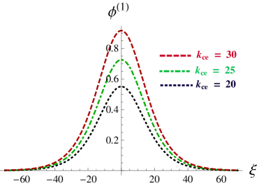
Figure 1: (Color online) Showing the variation of the positive potential of magnetized K-dV solitons $\phi^{(1)}$ with $k_{ce}$ for $\mu_{ce}>\mu_{c}$, $u_{0}=0.01$, $\sigma_{1}=2.5$, $\sigma_{2}=0.1$, $\mu_{he}=0.04$, $k_{he}=2$, $\delta=5$ and $\alpha=0.5$ .

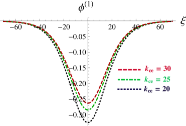
Figure 2: (Color online) Showing the variation of the negative potential of magnetized K-dV solitons $\phi^{(1)}$ with $k_{ce}$ for $\mu_{ce}<\mu_{c}$. The other plasma parameters are kept fixed.

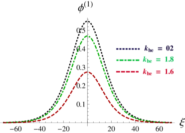
Figure 3: (Color online) Showing the variation of the positive potential of magnetized K-dV solitons $\phi^{(1)}$ with $k_{he}$ for $\mu_{ce}>\mu_{c}$ and $k_{ce}=20$. The other plasma parameters are kept fixed.

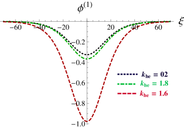
Figure 4: (Color online) Showing the variation of negative potential of magnetized K-dV solitons $\phi^{(1)}$ with $k_{he}$ for $\mu_{ce}<\mu_{c}$. The other plasma parameters are kept fixed.

Now, combining Eqs. (31) - (33) we obtain a equation of the form

$$\frac{\partial\phi^{(1)}}{\partial\tau}+\alpha_{1}\alpha_{3}\phi^{(1)2}\frac{\partial\phi^{(1)}}{\partial\xi}+\alpha_{2}\alpha_{3}\frac{\partial^{3}\phi^{(1)}}{\partial\xi^{3}}=0.$$ (34)

This is well-known mK-dV equation that describes the obliquely propagating HIA waves in a magnetized plasma. where $\alpha_{1}$, $\alpha_{2}$ and $\alpha_{3}$ are given by

$$\alpha_{1}=\frac{15L_{z}^{6}}{2V_{p}^{6}},$$ (35)

$$\alpha_{2}=1+\frac{(1-L_{z}^{2})}{\alpha^{2}},$$ (36)

$$\alpha_{3}=\frac{V_{p}^{3}}{2L_{z}^{2}}.$$ (37)

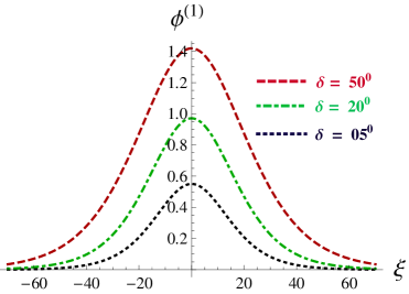
Figure 5: (Color online) Showing the variation of the positive potential of magnetized K-dV solitons $\phi^{(1)}$ with obliqueness $\delta$. The other plasma parameters are kept fixed.

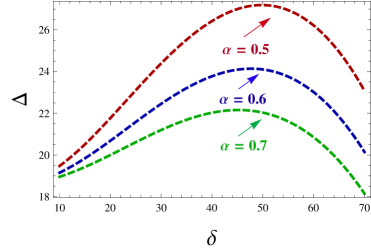
Figure 6: (Color online) Showing the variation of the width of magnetized K-dV solitons $\phi^{(1)}$ with $\alpha$. The other plasma parameters are kept fixed.

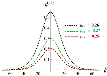
Figure 7: (Color online) Showing the variation of the amplitude of magnetized K-dV solitons with different values of $\mu_{ce}$. The other plasma parameters are kept fixed.

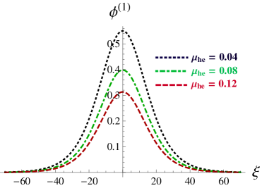
Figure 8: (Color online) Showing the variation of positive potential K-dV solitons with different values of $\mu_{he}$. The other plasma parameters are kept fixed.

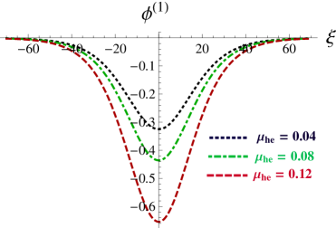
Figure 9: (Color online) Showing the variation of negative potential K-dV solitons with different values of $\mu_{he}$. The other plasma parameters are kept fixed except.

The stationary solitary wave solution of standard mK-dV equation is obtained by considering a frame $\xi=\eta-u_{0}T$ (moving with speed $u_{0}$) and the solution is,

$${\rm\phi^{(1)}}=\rm\phi_{m}{\rm[sech}(\frac{\xi}{\varpi})],$$ (38)

where the amplitude, $\phi_{m}=\sqrt{(6u_{0}/\alpha_{1}\alpha_{3})}$ and the width $\varpi=\phi_{m}{\sqrt{(\alpha_{1}/6)}}$.

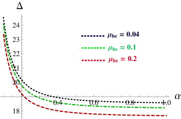
Figure 10: (Color online) Showing the variation of width (delta) of magnetized K-dV solitons with $\mu_{he}$ . The other plasma parameters are kept fixed.

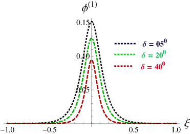
Figure 11: (Color online) Showing the variation of the amplitude of magnetized mK-dV solitons with with obliqueness $\delta$. The other plasma parameters are kept fixed.

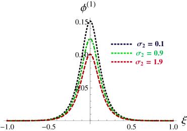
Figure 12: (Color online) Showing the variation of the amplitude of magnetized mK-dV solitons with $\sigma_{2}$ keeping other plasma parameters fixed.

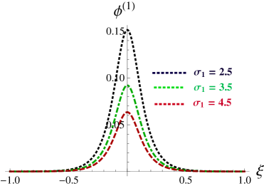
Figure 13: (Color online) Showing the variation of the amplitude of magnetized mK-dV solitons with $\sigma_{1}$ keeping other plasma parameters fixed.

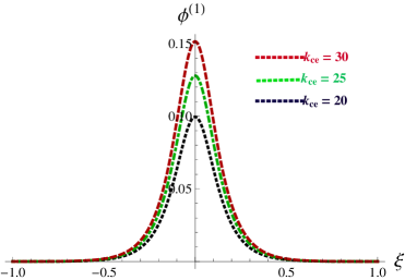
Figure 14: (Color online) Showing the variation of the amplitude of magnetized mK-dV solitons with $k_{ce}$ keeping other plasma parameters fixed.

Figure 15: (Color online) Showing the variation of the amplitude of magnetized fmK-dV compressive solitons with $k_{ce}$ keeping other plasma parameters fixed.

III.3 Derivation of the Magnetized further mK-dV Equation

In order to trace the vicinity of the critical heavy ion density, neither the magnetized KdV nor magnetized mKdV equation is suitable for describing the HIASWs. To examine the propagation of HIASWs in the vicinity of critical heavy ion density region, we assume a nonzero value for the ${\phi^{(1)}}^{2}$ of the Poisson’s equation and finally one can derive the following nonlinear equation

$$\frac{\partial\phi^{(1)}}{\partial\tau}+[\lambda\alpha_{3}\phi^{(1)}+\alpha_{1}{\alpha_{3}}^{2}\{\phi^{(1)}\}^{2}]\frac{\partial\phi^{(1)}}{\partial\xi}$$

$$\hskip 51.21495pt+\alpha_{3}\frac{\partial^{3}\phi^{(1)}}{\partial\xi^{3}}=0.$$ (39)

Eq. (39) is known as magnetized further mK-dV (fmK-dV) equation and the values of the constants are already mentioned in the previous. The compressive soliton solution (El-Shewy2011 ; Shah2015 ) of Eq. (39) is

$${\rm\phi^{(1)}_{+}}=\frac{6u_{0}/\lambda\alpha_{1}\alpha_{3}}{\phi^{(1)}sinh^{2}(\sqrt{u_{0}/2\lambda}\xi)-\phi^{(2)}cosh^{2}(\sqrt{u_{0}/2\lambda}\xi)},$$ (40)

and the rarefactive soliton solution (El-Shewy2011 ; Shah2015 )

$${\rm\phi^{(1)}_{-}}=\frac{6u_{0}/\lambda\alpha_{1}\alpha_{3}}{\phi^{(2)}sinh^{2}(\sqrt{u_{0}/2\lambda}\xi)-\phi^{(1)}cosh^{2}(\sqrt{u_{0}/2\lambda}\xi)}.$$ (41)

IV Discussion and Results

We have considered a magnetized plasma system consisting of inertial heavy ions and kappa distributed electrons of two distinct temperatures. We have derived the magnetized K-dV, mK-dV and fmK-dV-type partial differential equations by using the reductive perturbation method to investigate the basic features (i.e., amplitude, width and polarity etc.) of such a plasma system. The magnetized K-dV, mK-dV and fmK-dV equations are solved to set out the fascinating features of HIASWs. Then these solutions are analyzed by taking the effect of different plasma parameters like relative temperature-ratio of electrons (i.e., $\sigma_{1}$ and $\sigma_{2}$ ), superthermal parameter $k$ (i.e., $k_{ce}$ and $k_{he}$), relative electron number density ratio to heavy ion $\mu$ (i.e., $\mu_{ce}$ and $\mu_{he}$ ) etc. The results, which have been obtained from this theoretical investigation, can be pin-pointed as follows:

1. The magnetized K-dV and fmK-dV equations support HIA solitary waves with either compressive (positive) or rarefactive (negative) which depends on the critical value $\mu_{c}$, but for magnetized mK-dV equation only compressive SWs are formed.

2. We have numerically obtained here that for $\lambda=0$, the amplitude of the K-dV solitons become infinitely large, and the K-dV solution is no longer valid at $\lambda\simeq 0$. In our present investigation, we have found that for $\mu_{c}=\mu_{ce}=0.24$, the amplitude of the SWs breaks down due to the vanishing of the nonlinear coefficient $\lambda$. We have observed that at $\mu_{c}>0.24$, positive (compressive) potential SWs exist, whereas at $\mu_{c}<0.24$, negative (rarefactive) SWs exist (shown in Figs. 1-9).

3. It is observed that, the amplitude and width of both positive and negative potential magnetized K-dV SWs are totally depend on superthermal parameter of cold electron $k_{ce}$ and hot electron $k_{he}$. It is found that the amplitude and width of the positive and negative potential magnetized K-dV SWs increases with the increasing values of $k_{ce}$, as well as increasing the values of $k_{he}$ (shown in Figs. 1-4).

4. It is noticed that the amplitude and width of the positive potential of the magnetized K-dV soliton increases with the increase in obliqueness of the wave propagation $\delta$ (see Fig. 5).

5. It is observed that as the value of $\delta$ increases, the amplitude of the solitary waves increases, while their width increases for the lower range of $\delta$ (from $0^{\circ}$ to about $50^{\circ}$), and decreases for its higher range (from $50^{\circ}$ to about $90^{\circ}$). As $\delta\rightarrow 90^{\circ}$, the width goes to $0$, and the amplitude goes to $\infty$. It is likely that for large angles, the assumption that the waves are electrostatic is no longer valid, and we should look for fully electromagnetic structures. Our present investigation is only valid for small value of $\delta$ but invalid for arbitrary large value of $\delta$. In case of larger values of $\delta$, the wave amplitude becomes large enough to break the validity of the reductive perturbation method.

6. From the Fig. 6, it is seen that the amplitude and width of the solitary profile decreases with increasing values of number density ratio of cold electron to heavy ion $\mu_{ce}$.

7. It is found from Figs. 7 and 8, that the amplitude and width of both positive and negative potential magnetized K-dV SWs depend on the values of number density ratio of hot electron to heavy ion $\mu_{he}$. It is seen that the amplitude and width of the positive and negative potential magnetized K-dV SWs increases with the decreasing values of $\mu_{he}$.

8. Variation of the width of magnetized K-dV SWs for different values of $\mu_{he}$ with $\alpha$ is depicted in fig. 10. It is obtained that the width of magnetized K-dV SWs decreases with the increasing values of $\mu_{he}$.

9. In our present investigation, we have observed only positive potential magnetized mK-dV SWs. It is found that the amplitude and width of magnetized mK-dV SWs decreases with the increasing value of obliqueness $\delta$ (see Fig.11).

10. We have analyzed and found that the basic features of HIASWs depend on the relative temperature ratio of electrons(i.e., $\sigma_{1}$ and $\sigma_{2}$). It is found that the amplitude and width of magnetized mK-dV SWs decreases with the increasing value of $\sigma_{1}$ and $\sigma_{2}$ (see Figs. 12 and 13).

11. The variation of amplitude and width of magnetized mK-dV SWs which depends on superthermal parameter of cold electron $k_{ce}$ is depicted in Fig. 14. It is observed that the amplitude and width of magnetized mK-dV SWs decreases with the increasing value of $\sigma_{1}$ and $\sigma_{2}$.

12. The comparison among the K-dV, mK-dV and fmK-dV solitary amplitude is also important. It is observed that the amplitude of solitary waves decreases with the increasing of nonlinearities (see Figs. 1, 14, and 15).

In compressed, HIASWs have been studied in a magnetized space plasma. Since astrophysical objects are consists of heavy ions, the results of our present assessment can be applicable to the investigation on the HIASWs in such magnetized astrophysical objects including neutron stars, pulsar magnetosphere Kundu2011 , Saturn s magnetosphere Baluku2012 , peculiar velocities of galaxy clusters etc. where the effect of two temperature superthermal electrons play a crucial role.

V Acknowledgments

M. Sarker, B. Hosen and M. R. Hossen are profoundly grateful to the Ministry of Science and technology (Bangladesh) for awarding the National Science and Technology (NST) fellowship.

References

- (1) F. F. Chen, Introduction to Plasma Physics and Controlled Fusion, 2nd ed., Plenum Press, New York, p. 297 (1984).
- (2) I. R. Durrani, G. Murtaza, and H. U. Rahman, Can. J. Phys. 57, 642 (1979).
- (3) R. C. Davidson, Methods in Nonlinear Plasma Theory, Academic Press, New York, p. 15 (1972).
- (4) J. K. Chawla, M.K. Mishra, and R.S. Tiwary, Astrophys. Space Sci. 347, 283 (2013).
- (5) A. A. Mamun, Phys. Rev. E 55, 1852 (1997).
- (6) M. R. Hossen, L. Nahar, S. Sultana, and A. A. Mamun, Astrophys. Space Sci. 353, 123 (2014).
- (7) M. R. Hossen and A. A. Mamun, Braz. J. Phys. 44, 673 (2014).
- (8) M. R. Hossen, L. Nahar, and A. A. Mamun, J. Korean Phys. Soc. 65, 1863 (2014).
- (9) M. R. Hossen, L. Nahar, and A. A. Mamun, J. Astrophys. 2014, 653065 (2014).
- (10) B. Hosen, M. G. Shah, M. R. Hossen, and A. A. Mamun, Euro. Phys. J. Plus 131, 81 (2016).
- (11) M. J. Barlow, B. M. Swinyard, P. J. Owen, J. Cernicharo, H. L. Gomez, R. J. Ivison, O. Krause, T. L. Lim, M. Matsuura, S. Miller, G. Olofsson, and E. T. Polehampton, Science 342, 1343 (2013).
- (12) M. L. Burns, A. K. Harding, and R. Ramaty, Positron-electron Pairs in Astrophysics, American Institute of Physics, New York (1983).
- (13) F. C. Michel, Theory of Neutron Star Magnetosphere, Chicago University Press, Chicago (1991).
- (14) H. R. Miller and P. J. Witta, Active Galactic Nuclei, Springer, Berlin (1987).
- (15) P. Goldreich and W. H. Julian, Astrophys. J. 157, 869 (1969) .
- (16) M. J. Rees, In The Very Early Universe, eds. by G. W. Gibbons, S. W. Hawking, and S. Siklas, Cambridge University Press, Cambridge (1983).
- (17) K. E. Lonngren, Plasma Phys. 25, 943 (1983).
- (18) Y. Nakamura, J. L. Ferreira, and G. O. Ludwig, J. Plasma Phys. 33, 237 (1985).
- (19) Y. Nakamura, T. Ito, and K. Koga, J. Plasma Phys. 49, 331 (1993).
- (20) E. Witt and W. Lotko, Phys. Fluids 26, 2176 (1983).
- (21) S. Qian, W. Lotko, and M. K. Hudson, Phys. Fluids 31, 2190 (1988).
- (22) V. A. Marchenko and M. K. Hudson, J. Geophys. Res. 100, 19791 (1995).
- (23) C. Vocks and G. Mann, Astrophys. J. 593, 1134 (2003).
- (24) G. Gloeckler and L. A. Fisk, Astrophys. J. 648, L63 6 (2006).
- (25) Y. Yagi, V. Antoni, M. Bagatin, D. Desideri, E. Martines, G. Serianni, and F. Vallone, Plasma Phys. Cont. Fusion 39, 1915 (1997).
- (26) S. Preische, P. C. Efthimion and S. M. Kaye, Phys. Plasmas 3, 4065 (1996).
- (27) C. C. Chaston, Y. D. Hu, and B. J. Fraser, Geophys. Res. Lett. 24, 2913 (1997).
- (28) M. Maksimovic, V. Pierrard, and J. F. Lemaire, Astron. Astrophys. 324, 725 (1997).
- (29) V. M. Vasyliunas, J. Geophys. Res. 73, 2839 (1968).
- (30) D. Summers and R. M. Thorne, Phys. Fluids B 3, 1835 (1991).
- (31) M. A. Hellberg, R. L. Mace, T. K. Baluku, I. Kourakis, and N. S. Saini, Phys. Plasmas 16, 094701 (2009).
- (32) T. Cattaert, M. A. Helberg, and R. L. Mace, Phys. Plasmas 14, 082111 (2007).
- (33) M. S. Alam, M. M. Masud, and A. A. Mamun, Plasma Phys. Rep. 39, 1011 (2013).
- (34) B. Basu, Phys. Plasmas 15, 042108 (2008).
- (35) T. K. Baluku and M. A. Hellberg, Phys. Plasmas 19, 012106 (2012).
- (36) S. Hussain, Chin. Phys. Lett. 29, 065202 (2012).
- (37) M. Shahmansouri, B. Shahmansouri, and D. Darabi, Indian J. Phys. 87, 711 (2013).
- (38) S. Sultana and I. Kourakis, Plasma Phys. Control. Fusion 53, 045003 (2011).
- (39) P. Schippers et al., J. Geophys. Res. 113, A07208 (2008).
- (40) T. K. Baluku, M. A. Hellberg, and R. L. Mace, J. Geophys. Res. 116, A04227 (2011).
- (41) H. R. Pakzad, Astrophys. Space Sci. 331, 169 (2011).
- (42) I. Tasnim, M. M. Masud, M. Asaduzzaman, and A. A. Mamun, Chaos 23, 013147 (2013).
- (43) I. Tasnim, M. M. Masud, and A. A. Mamun, Astrophys. Space Sci. 343, 647 (2013).
- (44) M. M. Masud, S. Sultana, and A. A. Mamun, Astrophys. Space. Sci. 348, 99 (2013).
- (45) Q. M. Masud, S. Wang, and X. K. Dou, Astrophys. Space Sci. 12, 072903 (2005).
- (46) W. F. El-Taibany, N. A. El-Bedwehy, and E. F. El-Shamy, Phys. Plasmas 18, 033703 (2011).
- (47) M. Shahmansouri, Astrophys. Space Sci. 29, 105201 (2012).
- (48) S. A. Ema, M. R. Hossen, and A. A. Mamun, Phys. Plasmas 22, 092108 (2015).
- (49) S. A. Ema, M. R. Hossen, and A. A. Mamun, Contrib. Plasma Phys. 55, 596 (2015).
- (50) M. R. Hossen, L. Nahar, S. Sultana, and A. A. Mamun, High Energy Density Phys. 13, 13 (2014).
- (51) M. R. Hossen, L. Nahar, and A. A. Mamun, Phys. Scr. 89, 105603 (2014).
- (52) M. R. Hossen and A. A. Mamun, Plasma Sci. Technol. 17, 177 (2015).
- (53) M. G. Shah, M. M. Rahman, M. R. Hossen, and A. A. Mamun, Commun. Theor. Phys. 64, 208 (2015).
- (54) M. G. Shah, M. M. Rahman, M. R. Hossen, and A. A. Mamun, Plasma Phys. Rep. 42, 168 (2016).
- (55) S. A. Elwakil, E. M. Abulwafa, E. K. El-Shewy, and H. M. Abd-El-Hamid, Adv. Space Res. 48, 1578 (2011).
- (56) M. G. Shah, M. R. Hossen, and A. A. Mamun, J. Plasma Phys. 81, 905810517 (2015).
- (57) S. K. Kundu, D. K. Ghosh, P. Chatterjee, and B. Das Bulg. J. Phys. 38, 409 (2011).