Cell growth, division and death in cohesive tissues:
a thermodynamic approach

Abstract

Cell growth, division and death are defining features of biological tissues that contribute to morphogenesis. In hydrodynamic descriptions of cohesive tissues, their occurrence implies a non-zero rate of variation of cell density. We show how linear nonequilibrium thermodynamics allows to express this rate as a combination of relevant thermodynamic forces: chemical potential, velocity divergence, and activity. We illustrate the resulting effects of the non-conservation of cell density on simple examples inspired by recent experiments on cell monolayers, considering first the velocity of a spreading front, and second an instability leading to mechanical waves.

I Introduction

Biological tissues are assemblies of cells in mutual interaction Alberts et al. (2008). When cell-cell adhesion is strong and stable, cohesive tissues form continuous materials. Smooth mechanical fields can then be read from experimental data, among which the velocity Petitjean et al. (2010); Vig et al. (2016) and the stress field Ishihara and Sugimura (2012); Nier et al. (2016). Upon suitable coarse-graining over domains comprising several cells Bosveld et al. (2012), space-time maps of specific mesoscopic quantifiers can also be estimated in tissues, seen either as a cellular material (maps of cell area and anisotropy) or as a biomaterial (maps of cell division, death, and planar cell polarity).

Tissues differ from inert materials by the occurrence of cell division and death Alberts et al. (2008) and by the spontaneous generation of internal forces due to the activity of molecular motors and to nucleotide-dependent polymerization of cytoskeletal filaments Howard (2005). Since they contribute to morphogenesis Wolpert et al. (2006); Castanon and González-Gaitán (2011); Suzanne and Steller (2013); LeGoff and Lecuit (2015), cell growth, cell division and cell death must be included in hydrodynamic descriptions of tissues, in particular when the time scale considered is larger than a typical cell cycle.

Although the reaction of hydrolysis of adenosine triphosphate (ATP) is far from equilibrium ($\Delta\mu\simeq 25\,\mathrm{k}_{\mathrm{B}}T$ in usual conditions), linear non-equilibrium thermodynamics Chaikin and Lubensky (2000) has been shown to describe cytoskeletal mechanics with considerable success Kruse et al. (2005); Marchetti et al. (2013). In the same spirit, we apply linear non-equilibrium thermodynamics to a continuous material subject to cell growth, division and death, for which cell number density is not conserved (Sec. II). For illustrative purposes, we consider a viscoelastic cell monolayer in one spatial dimension Vedula et al. (2012); Yevick et al. (2015); Serra-Picamal et al. (2012); Tlili (2015); Peyret (2016). In Sec. III, we first investigate how cross-coefficients may modify the velocity of a moving free boundary during tissue expansion, before discussing in Sec. IV an example involving a polar order parameter, and examining the impact of cell division on the emergence of mechanical waves. Concerning terminology, cell “growth” refers to volumetric increase (or decrease) at fixed total cell number, and cell “death” includes non-lethal cell delamination from planar tissues. We do not consider the possible effects of cell division and death on tissue rheology, which may become relevant on time scales much larger than a typical cell cycle Ranft et al. (2010).

II Linear nonequilibrium thermodynamics

For simplicity, we consider a finite one-dimensional system of fixed size $L$, with spatial coordinate $x\in[0\;L]$ and time $t$. The cell number density field $\rho(x,t)$ obeys a balance equation with a source term due to cell growth, division and death, proportional to $\rho$:

$$\partial_{t}\rho+\partial_{x}\left(v\rho\right)=\kappa\,\rho\,.$$ (1)

This equation defines the rate of variation of the cell density $\kappa$, which we shall determine within the framework of linear nonequilibrium thermodynamics. We denote the tissue velocity and stress fields $v(x,t)$ and $\sigma(x,t)$, respectively. In the presence of an external force field $f_{\mathrm{ext}}$, the conservation of linear momentum reduces to the force balance equation:

$$\partial_{x}\sigma=-f_{\mathrm{ext}}\,,$$ (2)

since inertia is negligible at the length and velocity scales characteristic of tissue mechanics. We consider isothermal transformations at a constant, uniform temperature $T$. Given $f(\rho)$ the free energy density per unit length, we deduce the chemical potential $\mu=\left(\frac{\partial{f}}{\partial{\rho}}\right)_{T}$, and the pressure field $\pi=-f+\mu\rho$.

Eqs. (1-2) are supplemented by balance equations for the energy density $u$ and entropy density $s$:

$$\frac{\mathrm{d}{u}}{\mathrm{d}{t}} = -u\partial_{x}v-\partial_{x}j^{u}+f_{\mathrm{ext}}v\,,$$ (3)

$$\frac{\mathrm{d}{s}}{\mathrm{d}{t}} = -s\partial_{x}v-\partial_{x}j^{s}+\Sigma\,,$$ (4)

including density, energy and entropy currents $j^{\rho}$, $j^{u}$ and $j^{s}$ and the entropy production rate $\Sigma$. In 1D the total derivative is $\frac{\mathrm{d}{}}{\mathrm{d}{t}}=\frac{\partial{}}{\partial{t}}+v\frac{\partial{}}{\partial{x}}$. From the thermodynamic equality $\mathrm{d}u=T\mathrm{d}s+\mu\mathrm{d}\rho$, and identifying the pressure $\pi=-u+\mu\rho+Ts$, we obtain

$$T\,\Sigma = \frac{\mathrm{d}{u}}{\mathrm{d}{t}}-\mu\frac{\mathrm{d}{\rho}}{\mathrm{d}{t}}+Ts\partial_{x}v+T\partial_{x}j^{s}\,,$$ (5)

$$= \partial_{x}J-\mu\kappa\rho+\partial_{x}v\left(\sigma+\pi\right)-j^{\rho}\,\partial_{x}\mu\,,$$ (6)

using (1-4) and integrations by parts. The current $J=-j^{u}+Tj^{s}+\mu j^{\rho}-v\sigma$ contributes through a boundary term, and may thus be ignored in bulk. Among possible fluxes and forces, only $j^{\rho}$ and $\partial_{x}\mu$ change sign under the transformation $x\to-x$. At linear order, this forbids possible cross-couplings between $j^{\rho}$, $\partial_{x}\mu$ and other forces and fluxes. The diagonal term leads to Fickian diffusion Kruse et al. (2005), $j^{\rho}=-D\,\partial_{x}\rho$, irrelevant in the case of cohesive tissues. We therefore neglect the flux-force pair $(j^{\rho},-\partial_{x}\mu)$ from now on.

The hydrolysis of ATP is schematically represented as ATP $\to$ ADP $+\mathrm{P}_{\mathrm{i}}$. It proceeds at rate $r$, for a variation of chemical potential $\Delta\mu=\mu_{\mathrm{ATP}}-\mu_{\mathrm{ADP}}-\mu_{\mathrm{P}_{\mathrm{i}}}$, assumed to be constant. Taking into account ATP hydrolysis, we obtain the dissipation rate as the sum of thermodynamic flux-force products:

$$T\Sigma=\kappa\left(-\rho\mu\right)+\left(\sigma+\pi\right)\partial_{x}v+r\Delta\mu\,.$$ (7)

Despite its relevance for models of a dynamic, polymerizing and depolymerizing cytoskeleton, the term $\kappa\left(-\rho\mu\right)$ has not been studied explicitly in models of active matter Kruse et al. (2005); Doostmohammadi et al. (2015). Since $\left(-\rho\mu\right)$ can be computed from the free energy density, we treat it as a thermodynamic force and define the following flux-force pairs:

$$\begin{array}[]{ccc}\mathrm{Flux}&\leftrightarrow&\mathrm{Force}\\ \kappa&\leftrightarrow&-\rho\mu\\ \left(\sigma+\pi\right)&\leftrightarrow&\partial_{x}v\\ r&\leftrightarrow&\Delta\mu\end{array}$$

As discussed in Appendix A, choice of fluxes and forces has some arbitrariness in linear non-equilibrium thermodynamics, but this does not lead to essential differences in the resulting hydrodynamic equations.

To linear order, the constitutive equations read

$$\kappa = l_{11}\,\left(-\rho\mu\right)+l_{12}\,\partial_{x}v+\kappa_{\textrm{a}}$$ (8)

$$\sigma+\pi = -l_{12}\,\left(-\rho\mu\right)+\eta\,\partial_{x}v+\sigma_{\textrm{a}}\,,$$ (9)

where the diagonal coefficients $l_{11}$ and $l_{22}$ are non-negative, and Onsager relations have been applied. Since $r$ is not easily measurable, we ignore the analogous equation relating $r$ to the same forces. We recognize $\eta=l_{22}$ as the tissue viscosity, and $\sigma_{\textrm{a}}=l_{23}\,\Delta\mu$ as the active stress Kruse et al. (2005). The subscript $\mathrm{a}$ indicates that a parameter is active. We define an active rate $\kappa_{\textrm{a}}=l_{13}\,\Delta\mu$, which may be understood as a “swelling” rate Tlili et al. (2015), negative (respectively positive) when cell volume increases (respectively decreases). In the presence of cell growth, we define the homeostatic density $\rho_{\mathrm{h}}$ as the density at which cell growth, division and death balance each other in the absence of flow, i.e. $\kappa(\rho_{\mathrm{h}})=0$ with $v=\partial_{x}v=0$. Just as the active stress shifts the reference density at which the stress vanishes in the absence of viscous dissipation, the active rate shifts the homeostatic density (see Eqs. (13-14) for an example). Another approach Tlili et al. (2015) posits $\kappa$ as the sum of three rates, of cell growth, cell division, and cell death respectively. Since each process may be regulated by cell density and/or velocity divergence, and requires ATP hydrolysis for its completion, we expect the three rates to be functions of $\rho$, $\partial_{x}v$ and $\Delta\mu$. Only their sum $\kappa$ can be specified unambiguously by thermodynamics, Eq. (8).

The division rate has been observed experimentally to decrease with $\rho$ Folkman and Moscona (1978); Puliafito et al. (2012); Streichan et al. (2014). When divisions dominate $\kappa$, the positivity of $l_{11}$ implies that the chemical potential is negative and increases monotonically with $\rho$ (see examples below). For large values of the density (“overcrowding”), the chemical potential may become positive, whereby $\kappa$ becomes negative, indicating that cell delaminations dominate Eisenhoffer et al. (2012); Marinari et al. (2012). Through $-\rho\mu(\rho)$, $\kappa$ depends implicitly on the pressure $\pi(\rho)$, as proposed and investigated in the non-linear regime in Shraiman (2005). We expect $\kappa$ to be a decreasing function of pressure, as found experimentally to be caused either by an enhanced apoptotic rate Helmlinger et al. (1997) or by a reduced division rate Delarue et al. (2014), or by both Cheng et al. (2009). The rate of cell division also correlates with tissue contractility, while inhibitors of contractility alter spatial patterns of proliferation Nelson et al. (2005).

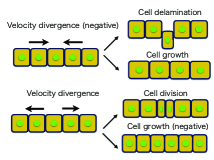
Figure 1: Schematic representation of the effect of the dimensionless cross-coefficient $l_{12}$ that couples cell growth, cell division and cell death to the velocity divergence ($l_{12}>0$).

Next, we explain the significance of the newly introduced dimensionless cross-coefficient $l_{12}$. Firstly, it couples the divergence of the tissue velocity to $\kappa$ as illustrated in Fig. 1. Observations of a positive correlation between a negative velocity divergence (“tissue convergence”) and cell delaminations (negative $\kappa$) Levayer et al. (2016) suggest that $l_{12}\geq 0$. Neglecting the influence of growth, divisions, and cell density variation, we roughly estimate $l_{12}\approx 10^{1}$ from the measurements of the cell delamination rate and tissue convergence in the fruitfly pupal midline Levayer et al. (2016). Secondly, substituting the expression of $-\rho\mu$ obtained from (8) into (9) allows to rewrite the stress field as:

$$\sigma=-\pi-\frac{l_{12}}{l_{11}}\kappa+\left(\eta+\frac{l_{12}^{2}}{l_{11}}\right)\,\partial_{x}v+\sigma_{\textrm{a}}+\frac{l_{12}}{l_{11}}\kappa_{\textrm{a}}\,,$$ (10)

implying that, through the cross-coefficient $l_{12}$, cell growth, division and death may modify the tissue mechanical behaviour, by changing its pressure, its viscosity and its active stress. In particular, we predict that $l_{12}$ increases the effective viscosity $\eta_{\mathrm{eff}}=\eta+\frac{l_{12}^{2}}{l_{11}}$ in general, and the effective pressure $\pi_{\mathrm{eff}}=\pi+\frac{l_{12}}{l_{11}}\kappa$ when $\kappa\geq 0$. A similar (shear) stress contribution due to cell divisions in 2D has been introduced phenomenologically to explain anisotropic growth in the fruitfly wing disk Bittig et al. (2009).

III First example: front velocity of an expanding cell monolayer

To illustrate the thermodynamic approach by a first concrete, yet simple example, let us consider the spreading of a cell monolayer in a quasi one-dimensional geometry, either within a channel Vedula et al. (2012), or along a linear fiber Yevick et al. (2015), and denote $L(t)$ its spatial extension at time $t$. Since it involves a free, moving boundary, this calculation is relevant to wound healing assays performed over long enough durations Murray (2002). The monolayer is compressible since the cell density decreases monotonically along $x$, and goes to zero at the free boundary, $x=L(t)$. Following Recho et al. (2016), we introduce the free energy density,

$$f\left(\rho\right)=E\left(\log\left(\frac{\rho_{\mathrm{e}}}{\rho}\right)+\frac{\rho}{\rho_{\mathrm{d}}}-1\right)$$ (11)

associated with two distinct reference cell densities $\rho_{\mathrm{e}}$ and $\rho_{\mathrm{d}}$. We deduce the chemical potential $\mu(\rho)=\frac{E}{\rho}\left(\frac{\rho}{\rho_{\mathrm{d}}}-1\right)$, the pressure field $\pi(\rho)=E\,\log\left(\frac{\rho}{\rho_{\mathrm{e}}}\right)$, and interpret in 1D the coefficient $E$ as an elastic modulus and $\rho_{\mathrm{e}}$ as a reference elastic density. The product $l_{11}E$ has the dimension of inverse time. Since $E\approx 10^{3}\,\mathrm{Pa}$ Harris et al. (2012) and $\tau_{\mathrm{h}}^{0}\approx 10^{4}\,\mathrm{s}$ Puliafito et al. (2012) we expect an order of magnitude for $l_{11}\approx 10^{-7}\,\mathrm{Pa^{-1}s^{-1}}$.

The external force $f_{\mathrm{ext}}=-\xi v$ is dissipative, with a positive friction coefficient $\xi$. An additional ingredient is the active boundary stress $\sigma_{\mathrm{p}}=\sigma\left(x=L(t),t\right)$, generated by the lamellipodial activity of leading cells, and assumed to be constant for simplicity. In the absence of cross-couplings ($l_{12}=\kappa_{\textrm{a}}=\sigma_{\textrm{a}}=0$), the “bare” homeostatic stress $\sigma_{h}^{0}=-E\log\left(\frac{\rho_{\mathrm{d}}}{\rho_{\mathrm{e}}}\right)$ is observed in bulk, where the tissue is under tension when $\rho_{\mathrm{d}}<\rho_{\mathrm{e}}$. Altogether, the free front may be pushed or pulled depending on the sign of the dimensionless control parameter

$$\alpha_{0}=\frac{\sigma_{\mathrm{p}}-\sigma_{h}^{0}}{E}=\frac{\sigma_{\mathrm{p}}}{E}+\log\left(\frac{\rho_{\mathrm{d}}}{\rho_{\mathrm{e}}}\right)\,,$$ (12)

leading to front motion at constant velocity $V$ Recho et al. (2016).

From (8-9-11), the constitutive equations read:

$$\kappa = l_{11}E\,\left(1-\frac{\rho}{\rho_{\mathrm{d}}}\right)+l_{12}\,\partial_{x}v+\kappa_{\textrm{a}}$$ (13)

$$\sigma = -E\log\left(\frac{\rho}{\rho_{\mathrm{e}}}\right)+l_{12}E\,\left(\frac{\rho}{\rho_{\mathrm{d}}}-1\right)+\eta\partial_{x}v+\sigma_{\textrm{a}}$$ (14)

The product $l_{11}E$ has the dimension of inverse time. We define the dimensionless active rate $\tilde{\kappa}_{\mathrm{a}}={\kappa_{\textrm{a}}}/{l_{11}E}$. A non-zero active rate $\kappa_{\textrm{a}}$ shifts the homeostatic density $\rho_{\mathrm{h}}$ from its “bare” value $\rho_{\mathrm{h}}^{0}=\rho_{\mathrm{d}}$ to $\rho_{\mathrm{h}}=\rho_{\mathrm{d}}\,\left(1+\tilde{\kappa}_{\mathrm{a}}\right)$, and the associated characteristic time $\tau_{\mathrm{h}}$ from $\tau_{\mathrm{h}}^{0}=\left(l_{11}E\right)^{-1}$ to $\tau_{\mathrm{h}}=\left(l_{11}E\right)^{-1}\left(1+\tilde{\kappa}_{\mathrm{a}}\right)^{-1}$. In the general case, the control parameter reads (see below)

$$\alpha=\frac{\sigma_{\mathrm{p}}-\sigma_{\textrm{a}}}{E}+\log\left(\frac{\rho_{\mathrm{d}}}{\rho_{\mathrm{e}}}\left(1+\tilde{\kappa}_{\mathrm{a}}\right)\right)-\tilde{\kappa}_{\mathrm{a}}l_{12}\,.$$ (15)

Although a detailed study of the influence of the parameters $l_{12}$ and $\kappa_{\textrm{a}}$ on front propagation at arbitrary driving is beyond the scope of this work, we extend a perturbative calculation of the front velocity $V$ done in Recho et al. (2016) for $l_{12}=\kappa_{\textrm{a}}=0$. For convenience, we introduce the following dimensionless quantities: $\hat{\rho}=\frac{\rho}{\rho_{\mathrm{h}}}$, $\hat{t}=\frac{t}{\tau_{\mathrm{h}}}$ $\hat{x}=x\sqrt{\frac{\xi}{E\tau_{\mathrm{h}}}}$ and $\hat{\sigma}=(\sigma-\sigma_{\mathrm{p}})/E$. The continuity and force balance equation now read

$$\partial_{t}\hat{\rho}+\partial_{\hat{x}}\left(\hat{v}\hat{\rho}\right)=\hat{\rho}\left(1-\hat{\rho}\right)+l_{12}\,\partial_{\hat{x}}\hat{v}$$ (16)

$$\partial_{\hat{x}}\hat{\sigma}=\hat{v}$$ (17)

with $\hat{\sigma}=-\log(\hat{\rho})+\tilde{l}_{12}\left(\hat{\rho}-1\right)+\tilde{\eta}\,\partial_{\hat{x}}\hat{v}-\alpha$, and the definitions $\tilde{\eta}=\frac{\eta}{E\tau_{\mathrm{h}}}$, $\tilde{l}_{12}=l_{12}\frac{\rho_{\mathrm{h}}}{\rho_{\mathrm{d}}}$, and where $\alpha$ is given by (15). Hereafter we shall omit the hats on dimensionless quantities (but not the tildes on dimensionless parameters). The boundary conditions for the scaled stress field are given by $\sigma\left(x=L\left(t\right),t\right)=0$, $\partial_{x}\sigma\left(x=L(t),t\right)=\dot{L}(t)$, $\partial_{x}\sigma\left(x=0,t\right)=0$.

We shall solve for the front velocity $V$ in steady front propagation for small $|\alpha|$. We denote the front position by $z=0$, where $z$ is defined as $z=x-Vt$. The conservation equations are

$$-V\rho^{\prime}+\left(\rho\sigma^{\prime}\right)^{\prime} = \rho\left(1-\rho\right)+l_{12}\,\sigma^{\prime\prime}$$

$$\tilde{\eta}\,\sigma^{\prime\prime}-\sigma = \log\rho+\tilde{l}_{12}\left(1-\rho\right)+\alpha\,,$$

where a ^′ denotes the derivative with respect to $z$, and the boundary conditions become $\sigma\left(z=0\right)=0$, $\sigma^{\prime}\left(z=0\right)=V$, $\lim_{z\to-\infty}\sigma^{\prime}\left(z\right)=0$.

We expand all variables and fields around the steady state obtained when $\alpha=0$: $\alpha=0+\epsilon\alpha_{1}$, $V=0+\epsilon V_{1}$, $\sigma(z)=0+\epsilon\sigma_{1}(z)$, $\rho(z)=1+\epsilon\rho_{1}(z)$. At order $\epsilon^{1}$, we find:

$$\sigma_{1}^{\prime\prime} = -\rho_{1}+l_{12}\,\sigma_{1}^{\prime\prime}$$

$$\tilde{\eta}\sigma_{1}^{\prime\prime}-\sigma_{1} = \rho_{1}(1-\tilde{l}_{12})+\alpha_{1}$$

and deduce the following differential equation for $\sigma_{1}$:

$$\left(\tilde{\eta}+(1-l_{12})(1-\tilde{l}_{12})\right)\,\sigma_{1}^{\prime\prime}-\sigma_{1}=\alpha_{1}\,.$$ (18)

As shown below, the quantity $\tilde{\eta}+(1-l_{12})(1-\tilde{l}_{12})$ must be positive for linear stability of the uniform bulk state $\rho=\rho_{\mathrm{h}},V=0$. A perturbation of small amplitude with wave number $q$ reads

$$\left(\rho(x,t),\sigma(x,t)\right)=\left(1,0\right)+\left(\delta\rho,\delta\sigma\right)\,e^{st-iqx}$$

with a growth rate $s$. Using Eqs. (16-17), we find at linear order,

$$s\delta\rho-q^{2}\delta\sigma = -\delta\rho-q^{2}l_{12}\,\delta\sigma\,,$$

$$-q^{2}\tilde{\eta}\,\delta\sigma-\delta\sigma = (1-\tilde{l}_{12})\delta\rho\,,$$

and determine the growth rate as

$$s(q)=-\frac{\tilde{\eta}+(1-l_{12})(1-\tilde{l}_{12})+1/q^{2}}{\tilde{\eta}+1/q^{2}}\,.$$

Linear stability ($s(q)<0,\forall q$) indeed requires the positivity of $\tilde{\eta}+(1-l_{12})(1-\tilde{l}_{12})$.

Solving (18), we obtain the expression of the stress profile

$$\sigma_{1}(z)=\alpha_{1}\left(e^{z/\sqrt{\tilde{\eta}+(1-l_{12})(1-\tilde{l}_{12})}}-1\right)\,,$$ (19)

from which we deduce the velocity and cell density profiles:

$$v_{1}(z) = \frac{\alpha_{1}}{\sqrt{\tilde{\eta}+(1-l_{12})(1-\tilde{l}_{12})}}e^{z/\sqrt{\tilde{\eta}+(1-l_{12})(1-\tilde{l}_{12})}}\qquad$$ (20)

$$\rho_{1}(z) = \frac{\alpha_{1}\,(l_{12}-1)}{\tilde{\eta}+(1-l_{12})(1-\tilde{l}_{12})}e^{z/\sqrt{\tilde{\eta}+(1-l_{12})(1-\tilde{l}_{12})}}\,.$$ (21)

The front velocity is calculated from the boundary condition $V_{1}=v_{1}\left(z=0\right)$. We find that in the limit of small driving $|\alpha|\ll 1$ and when $l_{12}\neq 0$, $\kappa_{\textrm{a}}\neq 0$, the dimensionless front velocity reads

$$\mathcal{V}=\frac{V}{\sqrt{\frac{E}{\xi\,\tau_{\mathrm{h}}^{0}}}}=\alpha\,\,\sqrt{\frac{1+\tilde{\kappa}_{\mathrm{a}}}{\tilde{\eta}+\left(1-l_{12}\right)\left(1-l_{12}\left(1+\tilde{\kappa}_{\mathrm{a}}\right)\right)}}\,,$$ (22)

as a function of $\alpha$, $l_{12}$, $\tilde{\kappa}_{\mathrm{a}}$, and $\tilde{\eta}=\frac{\eta}{E\tau_{\mathrm{h}}}$ the dimensionless viscosity. Since a finite homeostatic density requires $1+\tilde{\kappa}_{\mathrm{a}}>0$ (Eq. (13)), the argument of the square root in (22) is positive.

When $\kappa_{\textrm{a}}=0$, the driving $\alpha$ does not depend on $l_{12}$, which can adopt arbitrary large values while $|\alpha|\ll 1$. Since $\tilde{\eta}\approx 10^{-2}$ Recho et al. (2016), the front velocity is reduced by a factor close to $|l_{12}|$ when $|l_{12}|\gg 1$ and $\kappa_{\textrm{a}}=0$. When $\kappa_{\textrm{a}}\neq 0$, the driving $\alpha$ may remain small provided that $\kappa_{\textrm{a}}l_{12}$ is also small. Fig. 2 shows how $\mathcal{V}$ depends on the active rate $\kappa_{\textrm{a}}$ at fixed, small $\kappa_{\textrm{a}}l_{12}$, when $l_{12}\geq 0$ and $\alpha_{0}=0.2$ (reference velocity $\mathcal{V}_{0}\simeq\alpha_{0}=0.2$ when $l_{12}=\kappa_{\textrm{a}}=0$). A large enough, positive $\kappa_{\textrm{a}}$ increases $\mathcal{V}$ above $\mathcal{V}_{0}$, with a maximal value $\mathcal{V}_{\mathrm{max}}\gg\mathcal{V}_{0}$ reached close to $l_{12}=1$. A large, positive maximal velocity is also obtained for negative $\kappa_{\textrm{a}}$ close to $l_{12}=1$. Remarkably, a negative $\kappa_{\textrm{a}}$ may change the sign of the velocity as $\alpha$ becomes negative. We conclude that the sign and numerical value of the front velocity are sensitive to the cross-coefficients $l_{12}$ and $\kappa_{\textrm{a}}$, while $l_{11}$ determines the velocity scale.

The above expression of the front velocity (22), together with the profiles of stress, velocity and cell density, Eqs. (19-21) can be tested experimentally. Comparison with spreading assays where either cell division, cell apoptosis, and/or contractility are inhibited may lead to quantitative estimates of $l_{12}$ and $\tilde{\kappa}_{\mathrm{a}}$.

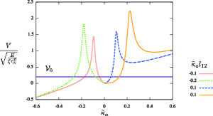
Figure 2: Dimensionless front velocity $\mathcal{V}=V/\sqrt{\frac{E}{\xi\,\tau_{\mathrm{h}}^{0}}}$ as a function of $\tilde{\kappa}_{\mathrm{a}}$ at fixed $\tilde{\kappa}_{\mathrm{a}}l_{12}=-0.2,-0.1,0.1,0.2$, assuming $l_{12}\geq 0$, with $\alpha_{0}=0.2$ and $\tilde{\eta}=10^{-2}$. The solid line indicates the reference velocity $\mathcal{V}_{0}=0.2$ when $l_{12}=\kappa_{\textrm{a}}=0$. Using $E\approx 10^{3}\,{\mathrm{P}a}$ Harris et al. (2012), $\xi\approx 10^{16}\,\mathrm{Pa}\,\mathrm{m}^{-2}$ s Cochet-Escartin et al. (2014) and $\tau_{\mathrm{h}}^{0}\approx 10^{4}$ s Puliafito et al. (2012), the velocity scale is $\sqrt{\frac{E}{\xi\,\tau_{\mathrm{h}}^{0}}}\approx 10\,\mu\mathrm{m}\,\mathrm{h}^{-1}$ Recho et al. (2016). See also Fig. 7 for the case $l_{12}<0$.

IV Second example: mechanical waves in a polar tissue

As a second example, we ask how pattern formation in a polar tissue is modified by cell growth, division and death, or more precisely how the location of bifurcation thresholds leading to wave patterns depends on $l_{11}$ and $l_{12}$. Active gel models are prone to instabilities driven by their active coefficients Kruse et al. (2005); Marchetti et al. (2013). Experimentally, propagating mechanical waves have been observed close to the moving boundary of expanding epithelial monolayers Serra-Picamal et al. (2012); Tlili (2015), as well as in the bulk of confined systems Peyret (2016), over time scales similar to or larger than the typical cell cycle. Whereas other models of an instability leading to mechanical waves consider an incompressible material Blanch Mercader (2014); Banerjee et al. (2015); Notbohm et al. (2016), we note that epithelial cell monolayers are compressible in 1D or 2D, with large fluctuations of cell sizes Serra-Picamal et al. (2012); Zehnder et al. (2015a, b). This observation justifies Eq. (1).

In motile cells, cell polarity arises from the distinct morphology of front and rear, from the inhomogeneous profiles of signaling molecules such as Rho and Rac, or from the respective positions of the cell centrosome and nucleus Mao and Lecuit (2016). Coarse-graining cell polarity at the tissue scale, we take into account a smooth polarity field $p(x,t)$ to describe the collective motion of a cohesive cell assembly. The constitutive equations of a polar material involve an additional flux-force pair $\dot{p}\leftrightarrow h$ Kruse et al. (2005), where $h$ is the field conjugate to $p$ and $\dot{p}=\partial_{t}+v\partial_{x}p$, see Eq. (34). Given the polar invariance of the tissue under $p\to-p$, $x\to-x$, Eqs. (8-9) generalize to

$$\kappa = l_{11}\,\left(-\rho\mu\right)+l_{12}\,\partial_{x}v+\kappa_{\textrm{a}}+\gamma_{\mathrm{a}}\partial_{x}p$$ (23)

$$\sigma+\pi = -l_{12}\,\left(-\rho\mu\right)+\eta\,\partial_{x}v+\sigma_{\textrm{a}}+\beta_{\mathrm{a}}\partial_{x}p$$ (24)

$$\dot{p} = \Gamma_{\mathrm{p}}h$$ (25)

where $\Gamma_{\mathrm{p}}\geq 0$. The active parameters $\beta_{\mathrm{a}}$ and $\gamma_{\mathrm{a}}$ couple thermodynamic fluxes to the polarity divergence.

To study quantitatively the mechanical waves observed in expanding tissues Serra-Picamal et al. (2012); Tlili (2015), one would need to combine both examples, e.g. associating the stress boundary condition at $x=L(t)$ to this analysis. Here, we focus on the question of how the emergence of waves is influenced by cell growth, division and death in bulk, and consider a system of fixed length $L$ with periodic boundary conditions, as may be realised in an annular geometry Nier et al. (2016). A minimal expression for the free energy density reads

$$f=\psi_{\rho}\left(\rho\right)+\psi_{\mathrm{p}}\left(p\right)+w\rho\,\partial_{x}p+\frac{\nu_{4}}{2}\left(\partial_{x}^{2}p\right)^{2}$$ (26)

including a quadratic function of the density

$$\psi_{\rho}\left(\rho\right)=\frac{1}{2K}\left(\frac{\rho-\rho_{\mathrm{e}}}{\rho_{\mathrm{e}}}\right)^{2}$$ (27)

that sets the reference elastic density $\rho_{\mathrm{e}}$, with a compressibility coefficient $K$; and a polarity-dependent term

$$\psi_{\mathrm{p}}\left(p\right)=-\frac{a_{2}}{2}p^{2}+\frac{a_{4}}{4}p^{4}$$ (28)

with $a_{2},a_{4}\geq 0$, that sets the reference polarity $p_{0}=\sqrt{a_{2}/a_{4}}$. As allowed by symmetry, the term $w\rho\,\partial_{x}p$ in (26) couples cell density and polarity divergence with a coefficient $w$ of unspecified sign Marcq (2014). The last term in (26) suppresses the instability at large wave numbers ($\nu_{4}\geq 0$) Chaikin and Lubensky (2000). Following Tlili (2015); Blanch Mercader (2014); Banerjee et al. (2015); Notbohm et al. (2016), we include an active motility term in the external force $f_{\mathrm{ext}}=-\xi v+f_{\mathrm{a}}p$ with a positive coefficient $f_{\mathrm{a}}$.

In the homogeneous state $p(x,t)=p_{0}$, $v(x,t)=v_{0}=f_{\mathrm{a}}p_{0}/\xi$, the density $\rho_{0}$ is determined by solving $\kappa(\rho_{0})=0$ or $\rho_{0}\,\mu(\rho_{0})=\kappa_{\textrm{a}}/l_{11}$. For simplicity, we set $\kappa_{\textrm{a}}=0$, so that $\rho_{0}=\rho_{\mathrm{e}}$, and consider small perturbations around $(\rho_{\mathrm{e}},p_{0},v_{0})$, see Eq. (35) in Appendix C. The growth rate of the instability is determined numerically from Eqs. (36-38). We find that the primary instability is a Hopf bifurcation, leading to traveling waves.

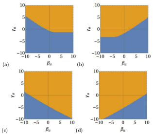
Figure 3: Stability diagram in the plane $(\beta_{\mathrm{a}},\gamma_{\mathrm{a}})$ of active control parameters for (a) $l_{11}=l_{12}=0$; (b) $l_{11}=0$, $l_{12}=2$; (c) $l_{11}=2$, $l_{12}=0$; (d) $l_{11}=l_{12}=2$. Orange (respectively blue) corresponds to a stable (respectively unstable) uniform state. Parameter values are: $\kappa_{\textrm{a}}=0$, $\eta=\sigma_{\textrm{a}}=\Gamma_{p}=w=\nu_{4}=K=\rho_{\mathrm{e}}=a_{2}=\xi=f_{\mathrm{a}}=1$ and $p_{0}=0.5$. See also Fig. 8 for the case $l_{12}=-2$.

With respect to the active control parameters $\beta_{\mathrm{a}}$ and $\gamma_{\mathrm{a}}$, bifurcation thresholds are sensitive to the coefficients $l_{11}$ and $l_{12}$ (see Fig. 3). In particular, we find that the instability is suppressed due to $l_{11}$. In the vanishing wavenumber limit, density perturbations obey $\left(s+\frac{l_{11}}{K}\right)\delta\rho=0$ (see Eq. (36)), and decouple from pressure and velocity perturbations. One solution for the growth rate is $s=-\frac{l_{11}}{K}<0$, suggesting that the source term in (1) stabilizes the uniform state through the coefficient $l_{11}$. Experimentally, pharmacological inhibition of cell division enhances waves in expanding monolayers Tlili (2015), in accord with our model. Since division and death are treated through the same field $\kappa$, this further suggests that inhibiting cell death would also enhance waves.

When $l_{11}=l_{12}=0$, Fig. 3a gives the bifurcation line in the $(\beta_{\mathrm{a}},\gamma_{\mathrm{a}})$ plane. Setting $l_{11}=0$, $l_{12}=2$ (Fig. 3b), the instability now occurs above a threshold value of $\beta_{\mathrm{a}}$ at fixed $\gamma_{\mathrm{a}}$, instead of below a threshold when $l_{11}=l_{12}=0$ (compare also Figs. 3c and 3d). An analytical calculation performed in the simpler case $\eta=l_{11}=f_{\mathrm{a}}=\gamma_{\mathrm{a}}=0$ (Appendix C.2) predicts that the bifurcation diagram depends on the sign of $w(1-l_{12})$, and thus on whether $l_{12}>1$ or $l_{12}<1$ (see Eq. (39)). In the general case, we observed numerically that smaller (respectively larger) $\beta_{\mathrm{a}}$ is favorable for the instability when $w(1-l_{12})>0$ (respectively $w(1-l_{12})<0$).

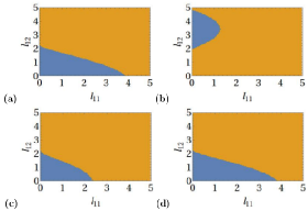
Figure 4: Stability diagrams in the plane $(l_{11},l_{12})$: (a) $\beta_{\mathrm{a}}=\gamma_{\mathrm{a}}=-5$; (b) $\beta_{\mathrm{a}}=10$, $\gamma_{\mathrm{a}}=5$. The color code and other parameter values are as in Fig. 3. See also Fig. 9 for the case $l_{12}<0$. Parameters in (c,d) are the same as in (a), with additional terms (c) $\alpha_{\mathrm{a}}=0,\nu_{2}=1$; (d) $\alpha_{\mathrm{a}}=1,\nu_{2}=0$.

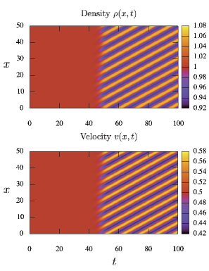
Figure 5: Numerical simulation Density and velocity fields obtained by numerical resolution of Eqs. (1-2, 23-25). Initial parameters $(l_{11},l_{12})=(1,3)$ are switched to $(l_{11},l_{12})=(1,1)$ when $t=10$ to induce an instability of the uniform state to a traveling wave. Other parameters are the same as in Fig. 4a.

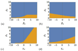
Figure 6: Stability diagrams in the $(\beta_{\mathrm{a}},\rho_{\mathrm{e}})$ plane, with (a) $l_{11}=0,l_{12}=0,\gamma_{\mathrm{a}}=0$; (b) $l_{11}=2,l_{12}=2,\gamma_{\mathrm{a}}=0$, and in the $(\gamma_{\mathrm{a}},\rho_{\mathrm{e}})$ plane, with (c) $l_{11}=0,l_{12}=0,\beta_{\mathrm{a}}=0$; (d) $l_{11}=2,l_{12}=2,\beta_{\mathrm{a}}=0$. The color code and other parameter values are as in Fig. 3.

At fixed values of the active parameters $\beta_{\mathrm{a}}$ and $\gamma_{\mathrm{a}},$ Fig. 4a indicates that $l_{12}$ also suppresses the instability. However, this is not general: reentrant behaviour as a function of $l_{12}$ is possible for other parameter values, see Fig. 4b. We briefly examined the cases including additional terms allowed by symmetry, such as an active transport term $\alpha_{\mathrm{a}}p\partial_{x}p$ in Eq. (25) or a lower-order gradient term $\frac{\nu_{2}}{2}\left(\partial_{x}p\right)^{2}$ in Eq. (26) (see Fig. 4cd). We present in Figs. 4cd the stability diagrams in the $(l_{11},l_{12})$ plane when either $\nu_{2}$ or $\alpha_{\mathrm{a}}$ is non-zero. As expected, the behavior is qualitatively the same as in Fig. 4a. Note however that $\nu_{2}$ suppresses somewhat the instability (Fig. 4c).

The validity of linear stability analysis was confirmed by numerical simulations. As an example, we present in Fig. 5 a numerical resolution of Eqs. (1-2, 23-25), supplemented with Eqs. (26-28), where we added to $\psi_{\rho}$ the fourth-order term $\frac{1}{4K_{4}}\left(\frac{\rho-\rho_{\mathrm{e}}}{\rho_{\mathrm{e}}}\right)^{4}$ with $K_{4}=1/400$ in order to saturate the instability. Starting the simulation with parameters for which the uniform state is linearly stable, we induce the formation of a traveling wave by changing the value of $l_{12}$, in agreement with linear stability analysis, see Fig. 4a.

Finally, we examined the cell density dependence of the stability threshold. We give the stability diagrams in Fig. 6. They indicate that a higher cell density is favorable for the instability in our model. In agreement with the general tendency found in Sec. C.2, the instability occurs for smaller $\beta_{\mathrm{a}}$ when $w(1-l_{12})>0$ and for larger $\beta_{\mathrm{a}}$ when $w(1-l_{12})<0$.

V Conclusion

To conclude, linear nonequilibrium thermodynamics specifies the rate of change of the cell density $\kappa$ as a linear combination of chemical potential, velocity divergence, activity, as well as polarity divergence when appropriate. In particular, the new cross-coefficient $l_{12}$ that couples $\kappa$ to the velocity divergence modifies cell monolayer mechanics, influencing the velocity of advancing fronts and altering pattern-forming instabilities. The decomposition (8) agrees qualitatively with a large body of experiments. Our results call for a careful quantitative comparison with experimental data, which will necessitate the simultaneous measurement in space and time and at tissue scale of several fields: the cell density, the velocity, the myosin distribution, and if possible the polarity.

In the case of elastic solids, growth has been studied with a careful treatment of thermodynamics, up to the regime of large deformations Ambrosi et al. (2011). As an advantage, our approach is easily generalizable to more complex rheologies including, e.g., orientational order parameters. Another advantage is that all the possible couplings are determined from symmetry without any ambiguity, at least in the regime of linear nonequilibrium. Extensions to 2 and 3 spatial dimensions are straightforward, where similar constitutive equations would apply to the isotropic parts of the relevant tensor fields, while, for instance, the couplings between mechanical fields and the orientation of cell division Castanon and González-Gaitán (2011) would pertain to their deviators. Our approach is applicable in vivo, where epithelial tissues such as the Drosophila pupal notum and wings are compressible in the plane Bosveld et al. (2012); Guirao et al. (2015).

Appendix A Choice of fluxes and forces

In linear nonequilibrium thermodynamics, the choice of force vs. flux is arbitrary, and can be modified at will thanks to a change of basis by standard linear algebra (see an example below). The choice made here:

$$\begin{array}[]{ccc}\mathrm{Flux}&\leftrightarrow&\mathrm{Force}\\ \kappa&\leftrightarrow&-\rho\mu\\ \left(\sigma+\pi\right)&\leftrightarrow&\partial_{x}v\\ r&\leftrightarrow&\Delta\mu\end{array}$$

is one of convenience, in order to express a poorly known quantity $\kappa$ as a function of quantities that are either measurable ($\partial_{x}v$) or computable once the free energy is given ($-\rho\mu$). We followed standard practice concerning the other flux-force pairs, with fluxes defined as $\sigma+\pi$ and $r$, see e.g. Kruse et al. (2005); Marchetti et al. (2013). Another approach Tlili et al. (2015) posits $\kappa$ as the sum of three rates, of cell growth, cell division, and cell death respectively. Since each process may be regulated by cell density and/or velocity divergence, and requires ATP hydrolysis for its completion, we expect the three rates to be functions of $\rho$, $\partial_{x}v$ and $\Delta\mu$. Only their sum $\kappa$ can be specified unambiguously by thermodynamics, Eq. (8).

Since the choice of fluxes and forces is arbitrary at linear order, it is for instance possible to rewrite our constitutive equation (see Eq. (10)) so that the cell density variation rate is expressed in terms of the stress, pressure and velocity divergence as

$$\kappa-\kappa_{\mathrm{a}}=-\frac{l_{11}}{l_{12}}\left(\sigma+\pi-\sigma_{\mathrm{a}}\right)+\left(l_{12}+\eta\frac{l_{11}}{l_{12}}\right)\partial_{x}v.$$ (29)

including also the active variables $\kappa_{\mathrm{a}}$ and $\sigma_{\mathrm{a}}$.

However, such transformations into another set of forces and fluxes become practically complicated when the Onsager coefficients depend on the hydrodynamic variables. Here, the only nonconstant Onsager coefficients that we include are related to activity/contractility (see the active terms in Eqs. (23-24)): the choice of $\Delta\mu$ as a force is non-trivial, but standard in the context of active gel models Kruse et al. (2005); Marchetti et al. (2013).

Finally, it would be possible to choose $-\mu$ as a force instead of $-\rho\mu$. Then the corresponding flux becomes $\kappa\rho$, and the hydrodynamic equations would be slightly modified. We may then rewrite Eqs. (8-9) as

$$\kappa\rho = l_{11}\,\left(-\mu\right)+l_{12}\partial_{x}v+\kappa_{\textrm{a}}$$ (30)

$$\sigma+\pi = -l_{12}\,\left(-\mu\right)+\eta\,\partial_{x}v+\sigma_{\textrm{a}}\,,$$ (31)

taking $\mu$ as a force. Since Onsager coefficients can have an arbitrary dependence on the hydrodynamic variable as far as positivity of the entropy production is guaranteed, if $l_{11}$, $l_{12}$ and $\kappa_{\textrm{a}}$ are functions of the cell density, we may obtain

$$\kappa\rho = l_{11}^{\prime}{\rho}^{2}\,\left(-\mu\right)+l_{12}^{\prime}\rho\,\partial_{x}v+\kappa_{\textrm{a}}^{\prime}\rho$$ (32)

$$\sigma+\pi = -l_{12}^{\prime}\rho\,\left(-\mu\right)+\eta\,\partial_{x}v+\sigma_{\textrm{a}}\,.$$ (33)

A different choice of force-flux pair may thus lead to the same hydrodynamic equations at the price of introducing density-dependent Onsager coefficients.

Appendix B Constitutive equations for a proliferating, compressible, active, and polar material

We consider in this section a system of constant size $L$ with periodic boundary conditions. Since the free energy of a polar material also depends on the polarity field and its spatial derivatives, $f=f(\rho,p,\partial_{x}p,\partial_{x}^{2}p)$, the calculation of the pressure and conjugate fields must be adapted. This is perhaps most easily seen by considering the free energy functional

$$F=\int_{0}^{L}\mathrm{d}x\,f(\rho,p,\partial_{x}p,\partial_{x}^{2}p)\,,$$

and computing its rate of variation:

$$\dot{F} = \frac{d}{dt}\int_{0}^{L}\mathrm{d}x\,f=\int_{0}^{L}\mathrm{d}x\,\partial_{t}f$$

$$= \int_{0}^{L}\mathrm{d}x\,\left(\frac{\mathrm{d}{f}}{\mathrm{d}{t}}-v\partial_{x}f\right)$$

$$= \int_{0}^{L}\mathrm{d}x\,\left(\frac{\mathrm{d}{f}}{\mathrm{d}{t}}+f\partial_{x}v\right)$$

$$= \int_{0}^{L}\mathrm{d}x\ \left(f\partial_{x}v+\frac{\partial{f}}{\partial{\rho}}\frac{\mathrm{d}{\rho}}{\mathrm{d}{t}}+\frac{\partial{f}}{\partial{p}}\frac{\mathrm{d}{p}}{\mathrm{d}{t}}+\right.$$

$$\left.\frac{\partial{f}}{\partial{(\partial_{x}p)}}\frac{\mathrm{d}{}}{\mathrm{d}{t}}\left(\partial_{x}p\right)+\frac{\partial{f}}{\partial{(\partial^{2}_{x}p)}}\frac{\mathrm{d}{}}{\mathrm{d}{t}}\left(\partial^{2}_{x}p\right)\right)$$

Since

$$\frac{\mathrm{d}{}}{\mathrm{d}{t}}\left(\partial_{x}p\right) =\partial_{x}\frac{\mathrm{d}{p}}{\mathrm{d}{t}}-(\partial_{x}p)(\partial_{x}v)$$

$$\frac{\mathrm{d}{}}{\mathrm{d}{t}}\left(\partial^{2}_{x}p\right) =\partial^{2}_{x}\frac{\mathrm{d}{p}}{\mathrm{d}{t}}-(\partial_{x}p)(\partial^{2}_{x}v)-2(\partial^{2}_{x}p)(\partial_{x}v)\,,$$

integrations by parts yield

$$\dot{F}=\int_{0}^{L}\mathrm{d}x\, \left\{\kappa\rho\frac{\partial{f}}{\partial{\rho}}\right.$$

$$+\dot{p}\left(\frac{\partial f}{\partial p}-\partial_{x}\left(\frac{\partial f}{\partial\left(\partial_{x}p\right)}\right)+\partial_{x}^{2}\left(\frac{\partial f}{\partial\left(\partial_{x}^{2}p\right)}\right)\right)$$

$$+\partial_{x}v\left(f-\rho\frac{\partial f}{\partial\rho}-\frac{\partial f}{\partial\left(\partial_{x}p\right)}\partial_{x}p-\frac{\partial f}{\partial\left(\partial_{x}^{2}p\right)}\partial_{x}^{2}p\right.$$

$$\left.\left.\vspace*{1cm}+\partial_{x}p\,\,\partial_{x}\left(\frac{\partial f}{\partial\left(\partial_{x}^{2}p\right)}\right)\right)\right\}$$

The power of the external force on the monolayer is

$$\Pi=\int_{0}^{L}\mathrm{d}x\,f_{\mathrm{ext}}v=-\int_{0}^{L}\mathrm{d}x\,v\partial_{x}\sigma=\int_{0}^{L}\mathrm{d}x\,\sigma\partial_{x}v\,.$$

Taking into account ATP hydrolysis, the dissipation rate $R$ reads

$$R = \Pi-\dot{F}+\int_{0}^{L}\mathrm{d}x\,r\Delta\mu$$ (34)

$$= \int_{0}^{L}\mathrm{d}x\left(-\rho\mu\kappa+\left(\sigma+\pi\right)\partial_{x}v+h\dot{p}+r\Delta\mu\right).$$

with

$$\mu = \frac{\partial f}{\partial\rho}\,,$$

$$\pi = -f+\rho\frac{\partial f}{\partial\rho}+\left(\frac{\partial f}{\partial\left(\partial_{x}p\right)}\right)\partial_{x}p-\partial_{x}\left(\frac{\partial f}{\partial\left(\partial_{x}^{2}p\right)}\right)\partial_{x}p$$

$$+\frac{\partial f}{\partial\left(\partial_{x}^{2}p\right)}\partial_{x}^{2}p\,,$$

$$h = -\frac{\partial f}{\partial p}+\partial_{x}\left(\frac{\partial f}{\partial\left(\partial_{x}p\right)}\right)-\partial_{x}^{2}\left(\frac{\partial f}{\partial\left(\partial_{x}^{2}p\right)}\right)\,.$$

Using (26) as the free energy density, we find

$$\mu = \psi^{\prime}_{\rho}(\rho)+w\partial_{x}p\,,$$

$$\pi = -f+\rho\psi^{\prime}_{\rho}{+2w\rho\partial_{x}p}+\nu_{4}\left[\left(\partial_{x}^{2}p\right)^{2}-\left(\partial_{x}p\right)\left(\partial_{x}^{3}p\right)\right]\,,$$

$$h = -\psi^{\prime}_{\mathrm{p}}\left(p\right)+w\partial_{x}\rho-\nu_{4}\partial_{x}^{4}p\,.$$

Appendix C Linear stability analysis

C.1 General case

Setting for simplicity $\kappa_{\textrm{a}}=0$, we study the linear stability of the uniform state $(\rho_{0},p_{0},v_{0})$ with $\rho_{0}=\rho_{\mathrm{e}}$ and $v_{0}=f_{\mathrm{a}}p_{0}/\xi$. A perturbation of small amplitude with wave number $q$ reads

$$\left(\rho,p,v\right)=\left(\rho_{\mathrm{e}},p_{0},v_{0}\right)+\left(\delta\rho,\delta p,\delta v\right)\,e^{st-iqx}$$ (35)

with a growth rate $s(q)$. Taking into account Eqs. (23-24) and (26-28), we find at linear order and with similar notations:

$$\delta(\rho\mu) = \frac{1}{K\rho_{\mathrm{e}}}\,\delta\rho-iqw\rho_{\mathrm{e}}\,\delta p$$

$$\delta\kappa = -\frac{l_{11}}{K\rho_{\mathrm{e}}}\delta\rho+iq\,(wl_{11}\rho_{\mathrm{e}}-\gamma_{\mathrm{a}})\delta p-iql_{12}\delta v$$

$$\hskip 14.22636pt\delta\pi = \frac{1}{K\rho_{\mathrm{e}}}\,\delta\rho-iqw{\rho_{\mathrm{e}}}\,\delta p$$

$$\delta\sigma = -\frac{L_{12}}{K\rho_{\mathrm{e}}}\,\delta\rho-iq\left(\beta_{\mathrm{a}}-L_{12}w{\rho_{\mathrm{e}}}\right)\,\delta p-iq\eta\delta v$$

$$\delta h = -iqw\,\delta\rho-\left(2a_{2}+\nu_{4}q^{4}\right)\,\delta p\,,$$

where $L_{12}=1-l_{12}$. Substituting into Eqs. (1-2-25), the amplitudes of perturbations obey at linear order:

$$\left(s+\frac{l_{11}}{K}-iqv_{0}\right)\,\delta\rho-iq{\rho_{\mathrm{e}}}\left(l_{11}w\rho_{\mathrm{e}}-\gamma_{\mathrm{a}}\right)\,\delta p-iq\rho_{\mathrm{e}}L_{12}\,\delta v = 0$$ (36)

$$\frac{iq}{K\rho_{\mathrm{e}}}L_{12}\,\delta\rho+\left(f_{\mathrm{a}}+q^{2}\left(L_{12}w\rho_{\mathrm{e}}-\beta_{\mathrm{a}}\right)\right)\,\delta p-\left(\xi+\eta q^{2}\right)\,\delta v = 0$$ (37)

$$iq\Gamma_{\mathrm{p}}w\,\delta\rho+\left(s+\Gamma_{\mathrm{p}}\left(2a_{2}+\nu_{4}q^{4}\right)-iqv_{0}\right)\,\delta p = 0$$ (38)

When $\mathrm{Re}(s)<0$ (respectively $\mathrm{Re}(s)>0$), the uniform state $\rho(x)=\rho_{0}$, $p(x)=p_{0}$, $v(x)=v_{0}$, is stable (respectively unstable). By evaluating numerically the largest real part of $s$, we obtain the stability diagrams plotted in figures.

C.2 Analytical calculation in a simple case

Setting $\eta=0$, $l_{11}=0$, $\gamma_{\mathrm{a}}=0$ and $f_{\mathrm{a}}=0$, an analytical expression of the stability threshold can be obtained. Contrary to the general case, the instability is here stationary, but this calculation is useful to understand the bifurcation diagrams in Fig. 3. The growth rate $s$ is a solution of the polynomial equation

$$\xi s^{2}+B\left(q^{2}\right)s+C\left(q^{2}\right)=0$$

with:

$$B\left(q^{2}\right) = \Gamma_{\mathrm{p}}\xi\nu_{4}\,q^{4}+\frac{(L_{12})^{2}}{K}\,q^{2}+2a_{2}\Gamma_{\mathrm{p}}\xi$$

$$C\left(q^{2}\right) = \frac{\Gamma_{\mathrm{p}}}{K}(L_{12})^{2}\nu_{4}\,q^{2}\,\times$$

$$\left[q^{4}-\frac{K\rho_{\mathrm{e}}}{\nu_{4}}w\left(w\rho_{\mathrm{e}}-\frac{\beta_{\mathrm{a}}}{L_{12}}\right)\,q^{2}+\frac{2a_{2}}{\nu_{4}}\right]$$

Since $B(q^{2})\geq 0$, the instability occurs when the minimum of $C\left(q^{2}\right)$ with respect to $q^{2}$ becomes negative, provided that

$$w\left(w\rho_{\mathrm{e}}-\frac{\beta_{\mathrm{a}}}{L_{12}}\right)>0.$$

Since the minimum of $C\left(q^{2}\right)$ is, up to a positive factor, proportional to

$$-\frac{1}{4}\left(\frac{K\rho_{\mathrm{e}}w}{\nu_{4}}\right)^{2}\left(w\rho_{\mathrm{e}}-\frac{\beta_{\mathrm{a}}}{L_{12}}\right)^{2}+2\frac{a_{2}}{\nu_{4}}\,,$$

the conditions for an instability are equivalent to

$$w\left(w\rho_{\mathrm{e}}-\frac{\beta_{\mathrm{a}}}{L_{12}}\right)>\frac{2}{\rho_{\mathrm{e}}K}\sqrt{2a_{2}\nu_{4}}\,.$$ (39)

Eq. (39) allows to define a threshold value $\beta_{\mathrm{a}}^{c}$ of the active parameter $\beta_{\mathrm{a}}$:

$$\beta_{\mathrm{a}}^{c}=L_{12}\left(w\rho_{\mathrm{e}}-\frac{2}{w\rho_{\mathrm{e}}K}\sqrt{2a_{2}\nu_{4}}\right)\,,$$

with two cases depending on the sign of the product $L_{12}w=(1-l_{12})w$.

If $(1-l_{12})w>0$ (respectively $(1-l_{12})w<0$ ), the instability takes place when $\beta_{\mathrm{a}}<\beta_{\mathrm{a}}^{c}$ (respectively $\beta_{\mathrm{a}}>\beta_{\mathrm{a}}^{c}$). This result agrees with the general tendency found numerically, and which holds in the general case $l_{11}\neq 0$, $f_{\mathrm{a}}\neq 0$, $\gamma_{\mathrm{a}}\neq 0$, that smaller (respectively larger) $\beta_{\mathrm{a}}$ is favorable for the instability when $(1-l_{12})w>0$ (respectively $(1-l_{12})w<0$).

The limit case $L_{12}=0$, $l_{12}=1$ leads to marginal stability (assuming as above that $\eta=l_{11}=\gamma_{\mathrm{a}}=f_{\mathrm{a}}=0$), with the growth rates $s=0$, $s=-\Gamma_{\mathrm{p}}\left(2a_{2}+\nu_{4}q^{4}\right)$, and may require a non-linear analysis.

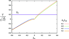
Figure 7: Dimensionless front velocity $\mathcal{V}=V/\sqrt{\frac{E}{\xi\,\tau_{\mathrm{h}}^{0}}}$ as a function of $\tilde{\kappa}_{\mathrm{a}}$ at fixed $\tilde{\kappa}_{\mathrm{a}}l_{12}=-0.2,-0.1,0.1,0.2$, assuming $l_{12}\leq 0$, with $\alpha_{0}=0.2$, $\tilde{\eta}=10^{-2}$. The solid line indicates the reference velocity at $l_{12}=\kappa_{\textrm{a}}=0$, $\mathcal{V}_{0}=\alpha_{0}/\sqrt{1+\tilde{\eta}}\simeq\alpha_{0}=0.2$.

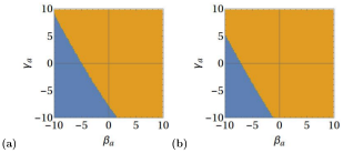
Figure 8: Stability diagrams in the plane $(\beta_{\mathrm{a}},\gamma_{\mathrm{a}})$ of active control parameters for (a) $l_{11}=0$, $l_{12}=-2$; (b) $l_{11}=2$, $l_{12}=-2$. The color code and other parameter values are as in Fig. 4.

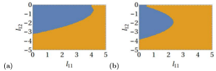
Figure 9: Stability diagrams in the plane $(l_{11},l_{12})$, with (a) $\beta_{\mathrm{a}}=-5$, $\gamma_{\mathrm{a}}=-5$; (b) $\beta_{\mathrm{a}}=-10$, $\gamma_{\mathrm{a}}=5$. The color code and other parameter values are as in Fig. 4.

Appendix D Cases with $l_{12}$ negative

As mentioned in the main text, experiments suggest that the cross-coupling $l_{12}$ is positive. Since linear nonequilibrium thermodynamics cannot exclude a negative sign for $l_{12}$, we briefly examine in this section, for each example, cases with a negative $l_{12}$

D.1 Front velocity for $l_{12}<0$

Fig. 7 shows how the dimensionless front velocity $\mathcal{V}$ depends on the active rate $\tilde{\kappa}_{\mathrm{a}}$ at fixed, small $\kappa_{\textrm{a}}l_{12}$, when $l_{12}<0$ and $\alpha_{0}=0.2$. $\mathcal{V}$ is a monotonically increasing function of $\tilde{\kappa}_{\mathrm{a}}$ except for $\tilde{\kappa}_{\mathrm{a}}$ close to $0$ and negative. A difference with the case $l_{12}\geq 0$ examined in the main text is the absence of a sharp peak, observed near $l_{12}=1$ in Fig. 2. Note that $\mathcal{V}$ rapidly changes sign to become negative fo $\tilde{\kappa}_{\mathrm{a}}<0$, $l_{12}<0$.

D.2 Stability analysis for $l_{12}<0$

We give the stability diagrams in the plane $(\beta_{\mathrm{a}},\gamma_{\mathrm{a}})$ for $l_{11}=0$, $l_{12}=-2$ (Fig. 8a) and $l_{11}=2$, $l_{12}=-2$ (Fig. 8b). A smaller $\beta_{a}$ is favorable for the instability in both cases with $l_{12}<0$, in accord with the general tendency for $w(1-l_{12})>0$ explained above. By comparing Fig. 8a and Fig. 8b, we see that the instability is suppressed due to $l_{11}$, as has also been observed in the main text in several cases with $l_{12}\geq 0$. Finally, we also observe reentrant behavior as a function of $l_{12}$ in the region $l_{12}<0$, see Fig. 9.