Runtime Verification of Temporal Properties over Out-of-order Data Streams

Abstract

We present a monitoring approach for verifying systems at runtime. Our approach targets systems whose components communicate with the monitors over unreliable channels, where messages can be delayed or lost. In contrast to prior works, whose property specification languages are limited to propositional temporal logics, our approach handles an extension of the real-time logic MTL with freeze quantifiers for reasoning about data values. We present its underlying theory based on a new three-valued semantics that is well suited to soundly and completely reason online about event streams in the presence of message delay or loss. We also evaluate our approach experimentally. Our prototype implementation processes hundreds of events per second in settings where messages are received out of order.

1 Introduction

Verifying systems at runtime can be accomplished by instrumenting system components so that they inform monitors about the actions they perform. The monitors update their states according to the information received and check whether the properties they are monitoring are fulfilled or violated. Various runtime-verification approaches exist for different kind of systems and property specification languages, see for example [2, 10, 18, 5, 21, 17, 7].

Many of these specifications languages are based on temporal logics or finite-state machines, which describe the correct system behavior in terms of infinite streams of system actions. However, at any point in time, a monitor has only partial knowledge about the system’s behavior. In particular, a monitor can at best only be aware of the previously performed actions, which correspond to a finite prefix of the infinite action stream. When communication channels are unreliable, a monitor’s knowledge about the previously performed actions may even be incomplete since messages can be lost or delayed and thus received out of order. Nevertheless, a monitor should output a verdict promptly when the monitored property is fulfilled or violated. Moreover, the verdict should remain correct when some of the monitor’s knowledge gaps are subsequently closed.

Many runtime-verification approaches rely on an extension of the standard Boolean semantics of the linear-time temporal logic LTL with a third truth value, proposed by Bauer et al. [9]. Namely, a formula evaluates to the Boolean truth value $b$ on a finite stream of performed actions $\sigma$ if the formula evaluates to $b$ on all infinite streams that extend $\sigma$; otherwise, the formula’s truth value is unknown on $\sigma$. This semantics, however, only accounts for settings where monitors are always aware of all previously performed actions. It is insufficient to reason soundly and completely about system behavior at runtime when, for example, unreliable channels are used to inform the monitors about the performed actions.

In this paper, we present an extension of the propositional real-time logic MTL [16, 1], which we name MTL^↓. First, MTL^↓ comprises a freeze quantifier [15] for reasoning about data values in action streams. The freeze quantifier $\downarrow$ can be seen as a restricted version of the first-order quantifiers $\exists$ and $\forall$. More concretely, at a position of the action stream, the formula $\mathop{\downarrow^{\!}}{\!x}\mathbin{\!.}\varphi$ uniquely binds a data value of the action at that position to the logical variable $x$.

Second, we equip MTL^↓ with a new three-value semantics that is well suited for settings where system components communicate with the monitors over unreliable channels. Specifically, we define the semantics of MTL^↓’s connectives over the three truth values $\mathsf{t}$, $\mathsf{f}$, and $\bot$. We interpret these truth values as in Kleene logic and conservatively extend the logic’s standard Boolean semantics, where $\mathsf{t}$ and $\mathsf{f}$ stand for “true” and “false” respectively, and the third truth value $\bot$ stands for “unknown” and accounts for the monitor’s knowledge gaps. The models of MTL^↓ are finite words where knowledge gaps are explicitly represented. Intuitively, a finite word corresponds to a monitor’s knowledge about the system behavior at a given time and the knowledge gaps may result from message delays, losses, crashed components, and the like. Critically in our setting, reasoning is monotonic with respect to the partial order on truth values, where $\bot$ is less than $\mathsf{t}$ and $\mathsf{f}$, and $\mathsf{t}$ and $\mathsf{f}$ are incomparable. This monotonicity property guarantees that closing knowledge gaps does not invalidate previously obtained Boolean truth values.

Third, we present an online algorithm for verifying systems at runtime with respect to MTL^↓ specifications. Our algorithm is based on, and extends, the algorithm for MTL by Basin et al. [6] to additionally handle the freeze quantifier. The algorithm’s output is sound and complete for MTL^↓’s three-valued semantics and with respect to the monitor’s partial knowledge about the performed actions at each point in time.

Our algorithm works roughly as follows. It receives messages from the system components describing the actions they perform. As with the algorithm in [6], no assumptions are made on the order in which messages are received. The algorithm updates its state for each received message. This state comprises a graph structure for reasoning about the system behavior, i.e., computing verdicts about the monitored property’s fulfillment. The graph’s nodes store the truth values of the subformulas at the different times for the data values to which quantified variables are frozen. In each update, the algorithm propagates data values down to the graph’s leaves and propagates Boolean truth values for subformulas up along the graph’s edges. When a Boolean truth value is propagated to a root node of the graph, the algorithm outputs a verdict.

Our main contribution is a runtime-verification approach that makes no assumptions about message delivery. It handles a significantly richer specification language than previous approaches, namely, an extension of the real-time logic MTL with a quantifier for reasoning about the data processed by the monitored system. Furthermore, our approach guarantees sound and complete reasoning with partial knowledge about system behavior. Finally, we experimentally evaluate the performance of a prototype implementation of our approach, illuminating its current capabilities, tradeoffs, and performance limitations.

The remainder of this paper is structured as follows. In Section 2, we introduce relevant notation and terminology. In Section 3, we extend MTL with the freeze quantifier and give the logic’s semantics. In Section 4, we describe our monitoring approach, including its algorithmic details. In Section 5, we report on our experimental evaluation. Finally, in Sections 6 and 7, we discuss related work and draw conclusions. Further details are given in the appendixes.

2 Preliminaries

In this section, we introduce relevant notation and terminology.

Intervals.

An interval $I$ is a nonempty subset of $\mathbb{Q}_{\geq 0}$ such that if $a,b\in I$ then $c\in I$, for any $c\in\mathbb{Q}_{\geq 0}$ with $a\leq c\leq b$. We use standard notation and terminology for intervals. For example, $(a,b]$ denotes the interval that is left-open with bound $a$ and right-closed with bound $b$. Note that an interval $I$ with cardinality $|I|=1$ is a singleton $\{\tau\}=[\tau,\tau]$, for some $\tau\in\mathbb{Q}_{\geq 0}$. An interval $I$ is unbounded if its right bound is $\infty$, and bounded otherwise. Let $I-J:=\{\tau-\tau^{\prime}\mathbin{\,|\,}\tau\in I\text{ and }\tau^{\prime}\in J\}\cap\mathbb{Q}_{\geq 0}$.

Partial Functions.

For a partial function $f:A\nrightarrow B$, let $\operatorname{def}(f):=\{a\in A\mathbin{\,|\,}f(a)\text{ is defined}\}$. If $\operatorname{def}(f)=\{a_{1},\dots,a_{n}\}$, for some $n\in\mathbb{N}$, we also write $[a_{1}\mapsto f(a_{1}),\dots,a_{n}\mapsto f(a_{n})]$ for $f$, when $f$’s domain $A$ and its codomain $B$ are irrelevant or clear from the context. Note that $[\,]$ denotes the partial function that is undefined everywhere. Furthermore, for partial functions $f,g:A\nrightarrow B$, we write $f\sqsubseteq g$ if $\operatorname{def}(f)\subseteq\operatorname{def}(g)$ and $f(a)=g(a)$, for all $a\in\operatorname{def}(f)$. We write $f[a\mapsto b]$ to denote the update of a partial function $f:A\nrightarrow B$ at $a\in A$, i.e., $f[a\mapsto b]$ equals $f$, except that $a$ is mapped to $b$ if $b\in B$, and $a\not\in\operatorname{def}(f[a\mapsto b])$ if $b\notin B$.

Truth Values.

Let $\mathsf{3}$ be the set $\{\mathsf{t},\mathsf{f},\bot\}$, where $\mathsf{t}$ (true) and $\mathsf{f}$ (false) denote the standard Boolean values, and $\bot$ denotes the truth value “unknown.” Table 1 shows the truth tables of some standard logical operators over $\mathsf{3}$. Observe that these operators coincide with their Boolean counterparts when restricted to the set $\mathsf{2}:=\{\mathsf{t},\mathsf{f}\}$.

Table 1: Truth tables for three-valued logical operators (strong Kleene logic).

$\neg$
$\mathsf{t}$	$\mathsf{f}$
$\mathsf{f}$	$\mathsf{t}$
$\bot$	$\bot$

$\vee$	$\mathsf{t}$	$\mathsf{f}$	$\bot$
$\mathsf{t}$	$\mathsf{t}$	$\mathsf{t}$	$\mathsf{t}$
$\mathsf{f}$	$\mathsf{t}$	$\mathsf{f}$	$\bot$
$\bot$	$\mathsf{t}$	$\bot$	$\bot$

$\wedge$	$\mathsf{t}$	$\mathsf{f}$	$\bot$
$\mathsf{t}$	$\mathsf{t}$	$\mathsf{f}$	$\bot$
$\mathsf{f}$	$\mathsf{f}$	$\mathsf{f}$	$\mathsf{f}$
$\bot$	$\bot$	$\mathsf{f}$	$\bot$

$\rightarrow$	$\mathsf{t}$	$\mathsf{f}$	$\bot$
$\mathsf{t}$	$\mathsf{t}$	$\mathsf{f}$	$\bot$
$\mathsf{f}$	$\mathsf{t}$	$\mathsf{t}$	$\mathsf{t}$
$\bot$	$\mathsf{t}$	$\bot$	$\bot$

We partially order the elements in $\mathsf{3}$ by their knowledge: $\bot\prec\mathsf{t}$ and $\bot\prec\mathsf{f}$, and $\mathsf{t}$ and $\mathsf{f}$ are incomparable as they carry the same amount of knowledge. Note that $(\mathsf{3},\prec)$ is a lower semilattice where $\curlywedge$ denotes the meet. We remark that the operators in Table 1 are monotonic. This ensures that reasoning is monotonic in knowledge. Intuitively, when closing a knowledge gap, represented by $\bot$, with $\mathsf{t}$ or $\mathsf{f}$, we never obtain a truth value that disagrees with the previous one.

Timed Words.

Let $\Sigma$ be an alphabet. A timed word over $\Sigma$ is an infinite word $(\tau_{0},a_{0})(\tau_{1},a_{1})\ldots\in(\mathbb{Q}_{\geq 0}\times\Sigma)^{\omega}$, where the sequence of $\tau_{i}$s is strictly monotonic and nonzeno, that is, $\tau_{i}<\tau_{i+1}$, for every $i\in\mathbb{N}$, and for every $t\in\mathbb{Q}_{\geq 0}$, there is some $i\in\mathbb{N}$ such that $\tau_{i}>t$.

3 Metric Temporal Logic Extensions

In this section, we extend the propositional real-time logic MTL [16, 1] with a freeze quantifier [15]. The logic’s three-valued semantics conservatively extends the standard Boolean semantics and accounts for knowledge gaps during monitoring.

3.1 Syntax

Let $P$ be a finite set of predicate symbols, where $\iota(p)$ denotes the arity of $p\in P$. Furthermore, let $V$ be a set of variables and $R$ a finite set of registers. The syntax of the real-time logic MTL^↓ is given by the grammar:

$$\varphi\mathbin{\ ::=\ }\mathsf{t}\mathbin{\,\big{|}\,}p(x_{1},\dots,x_{\iota(p)})\mathbin{\,\big{|}\,}\mathop{\downarrow^{\!r}}{\!x}\mathbin{\!.}\varphi\mathbin{\,\big{|}\,}\neg\varphi\mathbin{\,\big{|}\,}\varphi\vee\varphi\mathbin{\,\big{|}\,}\varphi\mathbin{\mathsf{U}}_{I}\varphi\,,$$

where $p\in P$, $x,x_{1},x_{2}\dots,x_{\iota(p)}\in V$, $r\in R$, and $I$ is an interval. For the sake of brevity, we limit ourselves to the future fragment and omit the temporal connective for “next.” A formula is closed if each variable occurrence is bound by a freeze quantifier. A formula is temporal if the connective at the root of the formula’s syntax tree is $\mathbin{\mathsf{U}}_{I}$. We denote by $\mathit{Sub}(\varphi)$ the set of $\varphi$’s subformulas.

We employ standard syntactic sugar. For example, $\varphi\rightarrow\psi$ abbreviates $(\neg\varphi)\vee\psi$, and $\operatorname{\text{\raisebox{-1.1pt}{\begin{turn}{45.0}\scalebox{0.9}{$\square$}\end{turn}}}}_{I}\varphi$ (“eventually”) and $\operatorname{\square}_{I}\varphi$ (“always”) abbreviate $\mathsf{t}\mathbin{\mathsf{U}}_{I}\varphi$ and $\neg\operatorname{\text{\raisebox{-1.1pt}{\begin{turn}{45.0}\scalebox{0.9}{$\square$}\end{turn}}}}_{I}\neg\varphi$, respectively. The nonmetric variants of the temporal connectives are also easily defined, e.g., $\operatorname{\square}\varphi:=\operatorname{\square}_{[0,\infty)}\varphi$. Finally, we use standard conventions concerning the connectives’ binding strength to omit parentheses. For example, $\neg$ binds stronger than $\wedge$, which binds stronger than $\vee$, and the connectives $\neg$, $\vee$, etc. bind stronger than the temporal connectives, which bind stronger than the freeze quantifier. To simplify notation, we omit the superscript $r$ in formulas like $\mathop{\downarrow^{\!r}}{\!x}\mathbin{\!.}\varphi$ whenever $r\in R$ is irrelevant or clear from the context.

Example 1

Before defining the logic’s semantics, we provide some intuition. The following formula formalizes the policy that whenever a customer executes a transaction that exceeds some threshold (e.g. $2,000) then this customer must not execute any other transaction for a certain period of time (e.g. 3 days).

$$\operatorname{\square}\mathop{\downarrow^{\!\mathit{cid}}}{\!c}\mathbin{\!.}\mathop{\downarrow^{\!\mathit{tid}}}{\!t}\mathbin{\!.}\mathop{\downarrow^{\!\mathit{sum}}}{\!a}\mathbin{\!.}\mathit{trans}(c,t,a)\wedge a\geq 2000\to\operatorname{\square}_{(0,3]}\mathop{\downarrow^{\!\mathit{tid}}}{\!t^{\prime}}\mathbin{\!.}\mathop{\downarrow^{\!\mathit{sum}}}{\!a^{\prime}}\mathbin{\!.}\neg\mathit{trans}(c,t^{\prime},a^{\prime})$$

We assume that the predicate symbol $\mathit{trans}$ is interpreted as a singleton relation or the empty set at any point in time. For instance, the interpretation $\{(\mathit{Alice},42,99)\}$ of $\mathit{trans}$ at time $\tau$ describes the action of $\mathit{Alice}$ executing a transaction with identifier $42$ with the amount $99 at time $\tau$. When the interpretation is the empty set, no transaction is executed. We further assume that when the interpretation of the predicate symbol $\mathit{trans}$ is nonempty, the registers $\mathit{cid}$, $\mathit{tid}$, and $\mathit{sum}$ store (a) the transaction’s customer, (b) the transaction identifier, and (c) the transferred amount, respectively. If the interpretation is the empty set, the registers store a dummy value, representing undefinedness.

The variables $c$, $t$, $a$, $t^{\prime}$, and $a^{\prime}$ are frozen to the respective register values. For example, $c$ is frozen to the value stored in the register $\mathit{cid}$ at each point in time and is used to identify later transactions from this customer. Furthermore, note that, e.g., the variables $t$ and $t^{\prime}$ are frozen to values stored in the registers $\mathit{tid}$ at different times. The freeze quantifier can be seen as a weak form of the standard first-order quantifiers [15]. Since a register stores exactly one value at any time, it is irrelevant whether we quantify existentially or universally over a register’s value. ∎

3.2 Semantics

MTL^↓’s models under the three-valued semantics are finite words (see Definition 1 below). Such a model represents a monitor’s partial knowledge about the system behavior at a given point in time. This is in contrast to the models for the standard Boolean semantics for MTL, which are infinite timed words and capture the complete system behavior in the limit.

Definition 1

Let $D$ be the data domain, a nonempty set of values with $\bot\not\in D$. Observations are finite words with letters of the form $(I,\sigma,\varrho)$, where $I$ is an interval, $\sigma:P\nrightarrow 2^{\bigcup_{\iota\in\mathbb{N}}D^{\iota}}$, and $\varrho:R\nrightarrow D$. We define observations inductively.

• The word $\big{(}[0,\infty),[\,],[\,]\big{)}$ of length $1$ is an observation.

• If $w$ is an observation, then the word obtained by applying one of the following transformations to $w$ is an observation.

  1. Some letter $(I,\sigma,\varrho)$ of $w$, where $|I|>1$, is replaced by the three-letter word ${\big{(}I\cap[0,\tau),\sigma,\varrho\big{)}}{\big{(}\{\tau\},\sigma,\varrho\big{)}}{\big{(}I\cap(\tau,\infty),\sigma,\varrho\big{)}}$, where $\tau\in I$ and $\tau>0$. If $\tau=0$, then $(I,\sigma,\varrho)$ is replaced by $\big{(}\{\tau\},\sigma,\varrho\big{)}\big{(}I\cap(\tau,\infty),\sigma,\varrho\big{)}$.

  2. Some letter $(I,\sigma,\varrho)$ of $w$, where $|I|>1$ and $I$ is bounded, is removed.

  3. Some letter $(I,\sigma,\varrho)$ of $w$, where $|I|=1$, is replaced by $(I,\sigma^{\prime},\varrho^{\prime})$, where $\sigma\sqsubseteq\sigma^{\prime}$ and $\varrho\sqsubseteq\varrho^{\prime}$, and $\sigma\neq\sigma^{\prime}$ or $\varrho\neq\varrho^{\prime}$.

For an observation $w$ of length $n\in\mathbb{N}$, let $\mathit{pos}(w):=\{0,\dots,n-1\}$. We call $i\in\mathit{pos}(w)$ a time point in $w$ if the interval $I_{i}$ of the letter at position $i$ in $w$ is a singleton. In this case, the element of $I_{i}$ is the timestamp of the time point $i$, denoted by $\operatorname{ts}_{w}(i)$. We note that for any letter $(I,\sigma,\varrho)$ of an observation, if $|I|>1$ then $\sigma=\varrho=[\,]$.

Example 2

A monitor’s initial knowledge is represented by the observation $w_{0}=\big{(}[0,\infty),[\,],[\,]\big{)}$. Suppose a transaction of $\$99$ with identifier $42$ from $\mathit{Alice}$ is executed at time $3.0$. The monitor’s initial knowledge $w_{0}$ is then updated by (T1) and (T3) to $w_{1}=\big{(}[0,3.0),[\,],[\,]\big{)}\big{(}\{3.0\},\sigma,\varrho\big{)}\big{(}(3.0,\infty),[\,],[\,]\big{)}$, where $\sigma(\mathit{trans})=\{(\mathit{Alice},42,99)\}$ and $\varrho=[\mathit{cid}\mapsto\mathit{Alice},\mathit{tid}\mapsto 42,\mathit{sum}\mapsto 99]$. If the monitor also receives the information that no action has occurred in the interval $[0,3.0)$, then its updated knowledge is represented by $\big{(}\{3.0\},\sigma,\varrho\big{)}\big{(}(3.0,\infty),[\,],[\,]\big{)}$, obtained from $w_{1}$ by (T2). The information that no action has occurred in an interval can be communicated explicitly or implicitly by the monitored system to the monitor, for instance, by attaching a sequence number to each action. See [6] for details. Finally, note that the interval of the last letter of any observation is always unbounded. This reflects that a monitor is unaware of what it will observe in the future. ∎

Definition 2

The observation $w^{\prime}$ refines the observation $w$, written $w{}_{1}w^{\prime}$, iff $w^{\prime}$ is obtained from $w$ by one of the transformations (T1), (T2), or (T3). The reflexive-transitive closure of ₁ is .

MTL^↓’s three-valued semantics is defined by a function $\varphi\mapsto\llbracket{w,i,\nu}\mathrel{|}\joinrel\approx{\varphi}\rrbracket\in\mathsf{3}$, for a given observation $w$, time point $i\in\mathbb{N}$, and partial valuation $\nu:V\nrightarrow D$. We define this function inductively over the formula structure. For a predicate symbol $p\in P$, we write in the following $p(\bar{x})$ instead of $p(x_{1},\dots,x_{\iota(p)})$. Furthermore, we abuse notation by abbreviating, e.g., $\nu(x_{1}),\dots,\nu(x_{n})$ as $\nu(\bar{x})$, for a partial valuation $\nu:V\nrightarrow D$ and variables $x_{1},\dots,x_{n}$. Also, the notation $\bar{x}\in\operatorname{def}(\nu)$ means that $x\in\operatorname{def}(\nu)$, for each $x$ occurring in $\bar{x}$. Finally, we identify the logic’s constant symbol $\mathsf{t}$ with the Boolean value $\mathsf{t}\in\mathsf{3}$, and the connectives $\neg$ and $\vee$ with the corresponding three-valued logical operators in Table 1.

$$\llbracket{w,i,\nu}\mathrel{|}\joinrel\approx{\mathsf{t}}\rrbracket:=\ \mathsf{t}$$

$$\llbracket{w,i,\nu}\mathrel{|}\joinrel\approx{p(\bar{x})}\rrbracket:=\ \begin{cases}\mathsf{t}&\text{if $\bar{x}\in\operatorname{def}(\nu)$, $p\in\operatorname{def}(\sigma_{i})$, and $\nu(\bar{x})\in\sigma_{i}(p)$}\\ \mathsf{f}&\text{if $\bar{x}\in\operatorname{def}(\nu)$, $p\in\operatorname{def}(\sigma_{i})$, and $\nu(\bar{x})\not\in\sigma_{i}(p)$}\\ \bot&\text{otherwise}\end{cases}$$

$$\llbracket{w,i,\nu}\mathrel{|}\joinrel\approx{\mathop{\downarrow^{\!r}}{\!x}\mathbin{\!.}\varphi}\rrbracket:=\ \llbracket{w,i,\nu[x\mapsto\varrho_{i}(r)]}\mathrel{|}\joinrel\approx{\varphi}\rrbracket$$

$$\llbracket{w,i,\nu}\mathrel{|}\joinrel\approx{\neg\varphi}\rrbracket:=\ \neg\llbracket{w,i,\nu}\mathrel{|}\joinrel\approx{\varphi}\rrbracket$$

$$\llbracket{w,i,\nu}\mathrel{|}\joinrel\approx{\varphi\vee\psi}\rrbracket:=\ \llbracket{w,i,\nu}\mathrel{|}\joinrel\approx{\varphi}\rrbracket\vee\llbracket{w,i,\nu}\mathrel{|}\joinrel\approx{\psi}\rrbracket$$

$$\llbracket{w,i,\nu}\mathrel{|}\joinrel\approx{\varphi\mathbin{\mathsf{U}}_{I}\psi}\rrbracket:=\ \textstyle\bigvee_{j\in\mathit{pos}(w),j\geq i}\Big{(}\mathrm{tp}_{w}(j)\wedge\mathrm{tc}_{w,I}(j,i)\wedge\llbracket{w,j,\nu}\mathrel{|}\joinrel\approx{\psi}\rrbracket\,\wedge$$

$$\qquad\qquad\qquad\qquad\qquad\textstyle\bigwedge_{i\leq k<j}\big{(}\mathrm{tp}_{w}(k)\rightarrow\llbracket{w,k,\nu}\mathrel{|}\joinrel\approx{\varphi}\rrbracket\big{)}\Big{)}$$

The auxiliary functions $\mathrm{tp}_{w}:\mathit{pos}(w)\rightarrow\mathsf{3}$ and $\mathrm{tc}_{w,I}:\mathit{pos}(w)\times\mathit{pos}(w)\rightarrow\mathsf{3}$, are defined as follows, where $I_{k}$ denotes the interval at position $k\in\mathit{pos}(w)$ in $w$.

$$\mathrm{tp}_{w}(j) :=\begin{cases}\mathsf{t}&\text{if $j$ is a time point in $w$}\\ \bot&\text{otherwise}\end{cases}$$

$$\mathrm{tc}_{w,I}(i,j) :=\begin{cases}\mathsf{t}&\text{if $\tau-\tau^{\prime}\in I$, for all $\tau\in I_{i}$ and $\tau^{\prime}\in I_{j}$}\\ \mathsf{f}&\text{if $\tau-\tau^{\prime}\notin I$, for all $\tau\in I_{i}$ and $\tau^{\prime}\in I_{j}$}\\ \bot&\text{otherwise}\end{cases}$$

We comment on the semantics of $\varphi\mathbin{\mathsf{U}}_{I}\psi$. The auxiliary functions account for the positions in $w$ that are not time points. For example, at position $i$, for a position $j\leq i$ to be a “valid anchor” for the formula, $j$ must be a time point (in this case $\mathrm{tp}_{w}(j)=\mathsf{t}$). Otherwise, the truth value $\bot$ is used to express that it is not yet known whether the interval at position $j$ in $w$ will contain a time point. Note that using the truth value $\mathsf{f}$ would be incorrect since a refinement of $w$ might contain a time point with a timestamp in $I_{j}$. Furthermore, $\mathrm{tc}_{w,I}(i,j)$ is used to account for the metric constraint of the temporal connective. In particular, $\mathrm{tc}_{w,I}(i,j)$ is $\bot$ if it is unknown in $w$ whether the formula’s metric constraint is always satisfied or never satisfied for the positions $i$ and $j$. Finally, suppose that $\varphi$’s truth value is $\mathsf{f}$ at a position $k$ between $j$ and $i$. If the interval $I_{k}$ at position $k$ is not a singleton, the function $\mathrm{tp}_{w}(k)$ “downgrades” this value to $\bot$, since it will be irrelevant in refinements of $w$ that do not contain any time points with timestamps in $I_{k}$.

Note that it may be the case that $\llbracket{w,i,\nu}\mathrel{|}\joinrel\approx{\varphi}\rrbracket\in\mathsf{2}$ when $i$ is not a time point in $w$ (i.e., $I_{i}$ is not a singleton). A trivial example is when $\varphi=\mathsf{t}$. In a refinement of $w$, it might turn out that there are no time points with timestamps in $I_{i}$, and hence a monitor should not output a verdict for the specification $\varphi$ at position $i$ in $w$. We address this artifact by downgrading (with respect to the partial order $\prec$) a Boolean truth value $\llbracket{w,i,\nu}\mathrel{|}\joinrel\approx{\varphi}\rrbracket$ to $\bot$ when $i$ is not a time point. To this end, we introduce the following variant of the semantics.

Definition 3

For a formula $\varphi$, an observation $w$, $\tau\in\mathbb{Q}_{\geq 0}$, and $\nu$ a partial valuation, we define $[{w,\tau,\nu}\mathrel{|}\joinrel\approx{\varphi}]:=\llbracket{w,i,\nu}\mathrel{|}\joinrel\approx{\varphi}\rrbracket$, provided that $\tau$ is the timestamp of some time point $i\in\mathit{pos}(w)$ in $w$, and $[{w,\tau,\nu}\mathrel{|}\joinrel\approx{\varphi}]:=\bot$, otherwise.

3.3 Properties

The following theorem states that MTL^↓’s three-valued semantics is monotonic in (on observations and partial valuations) and $\preceq$ (on truth values). This property is crucial for monitoring since it guarantees that a verdict output for an observation stays valid for refined observations.

Theorem 3.1

Let $\varphi$ be a formula, $\mu$ and $\nu$ partial valuations, $u$ and $v$ observations, and $\tau\in\mathbb{Q}_{\geq 0}$. If $u\sqsubseteq v$ and $\mu\sqsubseteq\nu$ then $[{u,\tau,\mu}\mathrel{|}\joinrel\approx{\varphi}]\preceq[{v,\tau,\nu}\mathrel{|}\joinrel\approx{\varphi}]$.

A similar theorem shows that MTL^↓’s three-valued semantics conservatively extends the standard Boolean semantics (see Appendix 0.A for details). Intuitively speaking, if a formula $\varphi$ evaluates to a Boolean value for an observation at time $\tau\in\mathbb{Q}_{\geq 0}$, then $\varphi$ has the same Boolean value at time $\tau$ for any timed word that refines the observation. Formally, a timed word $w^{\prime}$ refines an observation $w$, $w\sqsubseteq w^{\prime}$ for short, if for every $j\in\mathbb{N}$, there is some $i\in\mathit{pos}(w)$, such that $\tau_{j}\in I_{i}$, $\sigma_{i}\sqsubseteq\sigma^{\prime}_{j}$, and $\varrho_{i}\sqsubseteq\varrho^{\prime}_{j}$, where $(I_{\ell},\sigma_{\ell},\varrho_{\ell})$ and $(\tau_{k},\sigma^{\prime}_{k},\varrho^{\prime}_{k})$, for $\ell\in\mathit{pos}(w)$ and $k\in\mathbb{N}$, are the letters of $w$ and $w^{\prime}$, respectively.

We investigate next the decision problem that underlies monitoring.

Theorem 3.2

For an arbitrary formula $\varphi$, observation $w$, partial valuation $\nu$, time $\tau\in\mathbb{Q}_{\geq 0}$, and truth value $b\in\mathsf{2}$, the question of whether $[{w,\tau,\nu}\mathrel{|}\joinrel\approx{\varphi}]$ equals $b$ is $\mathrm{PSPACE}$-complete.

In a propositional setting, the corresponding decision problem can be solved in polynomial time using dynamic programming, where the truth values at the positions of an observation are propagated up the formula structure. Note that the truth value of a proposition at a position is given by the observation’s letter at that position. This is in contrast to MTL^↓, where atomic formulas can have free variables and their truth values at the positions in an observation $w$ may depend on the data values stored in the registers and frozen to these variables at different time points of $w$. Before truth values are propagated up, the bindings of variables to data values must be propagated down.

4 Monitoring Algorithm

In this section, we present an online algorithm that computes verdicts for MTL^↓ specifications. To support scalable monitoring, the computation is incremental in that, when refining an observation according to the transformations (T1)–(T3), the results from previous computations are reused, including the propagated data values and Boolean values. We also define correctness requirements for monitoring and establish the algorithm’s correctness.

4.1 Correctness Requirements

We define when a sequence of observations is valid for representing a monitor’s knowledge over time. We assume that the monitor receives in the limit infinitely many messages containing information about the system behavior. This assumption is invalid if the system ever terminates. Nevertheless, we make this assumption to simplify matters and it is easy to adapt the definitions and results to the general case.

Definition 4

The infinite sequence $\bar{w}=(w_{i})_{i\in\mathbb{N}}$ of observations is valid if $w_{0}=([0,\infty),[\,],[\,])$ and $w_{i}\sqsubsetneq w_{i+1}$, for all $i\in\mathbb{N}$.

Let $M$ be a monitor and $\bar{w}$ a valid sequence of observations. In the following, we view $w_{i}$ as the input to $M$ at iteration $i$. For the input $w_{i}$, $M$ outputs a set of verdicts, which is a finite set of pairs $(\tau,b)$ with $\tau\in\mathbb{Q}_{\geq 0}$ and $b\in\mathsf{2}$. We denote this set by $M(w_{i})$. Note that in practice, $M$ would receive at iteration $i>0$ a message that describes just the differences between $w_{i-1}$ and $w_{i}$. Furthermore, the $w_{i}$s can be understood as abstract descriptions of $M$’s states over time, representing $M$’s knowledge about the system behavior, where $w_{0}$ represents $M$’s initial knowledge. Also note that if the timed word $v$ is the system behavior in the limit, then $w_{i}\sqsubseteq v$, for all $i\in\mathbb{N}$, assuming that components do not send bogus messages. However, for every $i\in\mathbb{N}$, there are infinitely many timed words $u$ with $w_{i}\sqsubseteq u$. Since messages sent to the monitor can be lost, it can even be the case that there are timed words $u$ with $u\not=v$ and $w_{i}\sqsubseteq u$, for all $i\in\mathbb{N}$.

Definition 5

Let $M$ be a monitor, $\varphi$ a formula, and $\bar{w}$ a valid observation sequence.

• $M$ is observationally sound for $\bar{w}$ and $\varphi$ if for all partial valuations $\nu$ and $i\in\mathbb{N}$, if $(\tau,b)\in M(w_{i})$ then $[{w_{i},\tau,\nu}\mathrel{|}\joinrel\approx{\varphi}]=b$.

• $M$ is observationally complete for $\bar{w}$ and $\varphi$ if for all partial valuations $\nu$, $i\in\mathbb{N}$, and $\tau\in\mathbb{Q}_{\geq 0}$, if $[{w_{i},\tau,\nu}\mathrel{|}\joinrel\approx{\varphi}]\in\mathsf{2}$ then $(\tau,b)\in\bigcup_{j\leq i}M(w_{j})$, for some $b\in\mathsf{2}$.

We say that $M$ is observationally sound if $M$ is observational sound for all valid observation sequences and formulas $\varphi$. The definition of $M$ being observationally complete is analogous.

It follows from Theorem 3.2 that there exist monitors for MTL^↓ that are both observationally sound and complete. This is in contrast to correctness requirements that demand that a monitor outputs a verdict as soon as the specification has the same Boolean value on every extension of the monitor’s current knowledge. It is easy to see that, for a given specification language, such monitoring is at least as hard as checking satisfiability for the language. The propositional fragment of MTL^↓ is already undecidable [20]. Thus monitors satisfying such strong requirements do not exist for MTL^↓. For LTL, such stronger requirements are standardly formalized using a three-valued “runtime-verification” semantics, as introduced by Bauer et al. [10], and adopted by other runtime-verification approaches, e.g. [8]. See Appendix 0.A.2 for a formal definition of these requirements in our setting.

Example 3

Consider the formula $\varphi=\operatorname{\square}(p\wedge\operatorname{\text{\raisebox{-1.1pt}{\begin{turn}{45.0}\scalebox{0.9}{$\square$}\end{turn}}}}\neg p)$. Under the classical Boolean semantics, $\varphi$ is logically equivalent to $\mathsf{f}$, however not under our semantics. For example, $\llbracket{w,0,\nu}\mathrel{|}\joinrel\approx{\varphi}\rrbracket=\bot$, for $w=\big{(}[0,\infty),[\,],[\,]\big{)}$ and any valuation $\nu$. Given a valid observation sequence $\bar{w}$, an observationally sound and complete monitor for $\bar{w}$ and $\varphi$ will first output the verdict $(0,\mathsf{f})$ for the minimal $i$ such that $w_{i}$ contains a letter that assigns $p$ to false. ∎

4.2 Monitoring Algorithm

We sketch the algorithm’s state, its main procedure, and its main data structure. We provide further algorithmic details in Appendix 0.B.

4.2.1 Monitor State.

Before explaining the algorithm, we first rephrase the MTL^↓’s semantics such that it is closer to the representation used by the monitor. Given an $i\in\mathbb{N}$, a position $j\in\mathit{pos}(w_{i})$, and a subformula $\gamma$ of $\varphi$, we denote by $\Phi_{i}^{\gamma,J_{j}}$, where $J_{k}$ is the interval of the $k$th letter of $w_{i}$, the propositional formula:

$$\Phi_{i}^{\gamma,J_{j}}:=\left\{\begin{array}[]{l@{\quad}l}\gamma^{J_{j}}&\text{if $\gamma$ is atomic}\\ \neg\alpha^{J_{j}}&\text{if $\gamma=\neg\alpha$}\\ \alpha^{J_{j}}\lor\beta^{J_{j}}&\text{if $\gamma=\alpha\lor\beta$}\\ \alpha^{J_{j}}&\text{if $\gamma=\mathop{\downarrow^{\!r}}{\!x}\mathbin{\!.}{\alpha}$}\\ \bigvee_{k\geq j}\big{(}\mathit{tp}^{J_{k}}\land\mathit{tc}^{J_{k},J_{j}}_{\gamma}\land\beta^{J_{k}}\land\bigwedge_{j\leq h<k}(\mathit{tp}^{J_{h}}\to\alpha^{J_{h}})\big{)}&\text{if $\gamma=\alpha\mathbin{\mathsf{U}}_{I}\beta$},\end{array}\right.$$

where $\alpha^{K}$, $\mathit{tp}^{K}$, and $\mathit{tc}^{H,K}_{\psi}$ denote atomic propositions, for each proper subformula $\alpha$ of $\varphi$, each temporal subformula $\psi$ of $\varphi$, and all intervals $H,K$ of letters in $w_{i}$. Next, we define, for any partial valuation $\nu$, the substitution $\theta_{i}^{\nu}$ of Boolean values for these atomic propositions as follows:

$$\begin{array}[]{rl@{\quad}l}\theta_{i}^{\nu}(\alpha^{J_{j}}):=&\llbracket{w_{i},j,\nu}\mathrel{|}\joinrel\approx{\alpha}\rrbracket&\text{if $\llbracket{w_{i},j,\nu}\mathrel{|}\joinrel\approx{\alpha}\rrbracket\in\mathsf{2}$},\\ \theta_{i}^{\nu}(\mathit{tp}^{J_{j}}):=&\mathrm{tp}_{w_{i}}(j)&\text{if $\mathrm{tp}_{w_{i}}(j)\in\mathsf{2}$},\\ \theta_{i}^{\nu}(\mathit{tc}_{\alpha\mathbin{\mathsf{U}}_{I}\beta}^{J_{j},J_{k}}):=&\mathrm{tc}_{w_{i},I}(j,k)&\text{if $\mathrm{tc}_{w_{i},I}(j,k)\in\mathsf{2}$},\end{array}$$

and $\theta_{i}^{\nu}$ is undefined otherwise. In what follows, the symbol $\equiv$ denotes semantic equivalence between propositional formulas. It is easy to see that

$$\theta_{i}^{\mu}(\Phi_{i}^{\gamma,J_{j}})\equiv\llbracket{w_{i},j,\nu}\mathrel{|}\joinrel\approx{\gamma}\rrbracket\quad\text{iff}\quad\llbracket{w_{i},j,\nu}\mathrel{|}\joinrel\approx{\gamma}\rrbracket\in\mathsf{2},$$

where $\mu=\nu[x\mapsto\varrho_{j}(r)]$ if $\gamma=\mathop{\downarrow^{\!r}}{\!x}\mathbin{\!.}{\alpha}$ and $\mu=\nu$ otherwise, with $\varrho_{j}$ being the third component of the $j$th letter of $w_{i}$. Note that the formula $\theta_{i}^{\mu}(\Phi_{i}^{\gamma,J_{j}})$ tells us more than the truth value $\llbracket{w_{i},j,\nu}\mathrel{|}\joinrel\approx{\gamma}\rrbracket$. Indeed, when $\theta_{i}^{\mu}(\Phi_{i}^{\gamma,J_{j}})\not\equiv b$, for each $b\in\mathsf{2}$, then we know not only that $\llbracket{w_{i},j,\nu}\mathrel{|}\joinrel\approx{\gamma}\rrbracket=\bot$, but we also know what the causes of uncertainty are, namely the direct subformulas $\alpha$ of $\gamma$ and indexes $k$ with $\llbracket{w_{i},k,\mu}\mathrel{|}\joinrel\approx{\alpha}\rrbracket=\bot$.

The monitor maintains as state between its iterations a variant of the propositional formulas $\theta_{i}^{\mu}(\Phi_{i}^{\gamma,J_{j}})$. The reason for using variants is that it is not algorithmically convenient to transform $\theta_{i}^{\mu}(\Phi_{i}^{\gamma,J})$ into $\theta_{i+1}^{\mu}(\Phi_{i+1}^{\gamma,K})$, where $K$ is an interval (of a letter) in $w_{i+1}$ that originates from the interval $J$ in $w_{i}$. Such a transformation is needed for obtaining an incremental monitoring algorithm that reuses information already computed at previous iterations.

The formulas that the monitors maintains, denoted $\Psi_{i}^{\gamma,J_{j},\nu}$, can be obtained from the formulas $\theta_{i}^{\mu}(\Phi_{i}^{\gamma,J_{j}})$ as follows. When $\gamma$ is a nontemporal formula, then $\Psi_{i}^{\gamma,J_{j},\nu}$ equals $\theta_{i}^{\mu}(\Phi_{i}^{\gamma,J_{j}})$. When $\gamma$ is a temporal formula $\alpha\mathbin{\mathsf{U}}_{I}\beta$, then, to each disjunct for index $k$ in $\Phi_{i}^{\gamma,J_{j}}$, we add the subformula $(\mathit{tp}^{J_{k}}\lor\alpha^{J_{k}})$ as a conjunct. This is sound, based on the equivalence $\mathit{tp}^{J_{k}}\equiv\mathit{tp}^{J_{k}}\land(\mathit{tp}^{J_{k}}\lor\alpha^{J_{k}})$. Furthermore, the monitor treats the subformulas $(\mathit{tp}^{J_{k}}\land\beta^{J_{k}})$, $(\mathit{tp}^{J_{h}}\to\alpha^{J_{h}})$, and $(\mathit{tp}^{J_{k}}\lor\alpha^{J_{k}})$ in a special way: they are not simplified in $\Psi_{i}^{\gamma,J,\nu}$ when they are still needed to obtain $\Psi_{i+1}^{\gamma,K,\nu}$. That is, even if one the atomic propositions $q$ of these subformulas could be instantiated (i.e. $q\in\operatorname{def}(\theta_{i}^{\mu})$) this is not always done, as explained in the next section. Instead, these three types of subformulas are represented in $\Psi_{i}^{\gamma,J_{j},\nu}$ by the atomic propositions $\bar{\beta}^{J_{k}}$, $\bar{\alpha}^{J_{h}}$, and $\bar{\bar{\alpha}}^{J_{k}}$, respectively.

Example 4

We illustrate here the definitions of the propositional formulas $\Phi_{i}^{\gamma,J,\nu}$ and $\Psi_{i}^{\gamma,J,\nu}$ for temporal formulas $\gamma$. We also suggest why variants of the formulas $\theta_{i}^{\mu}(\Phi_{i}^{\gamma,J_{j}})$ are needed.

Let $\gamma=p\mathbin{\mathsf{U}}q$, where $p$ and $q$ are $0$-ary predicates. Assume that in $w_{1}$ we have the intervals $L=[0,\tau_{1})$, $N=\{\tau_{1}\}$, and $R=(\tau_{1},\infty)$, and in $w_{2}$ we have the intervals $L_{1}=[0,\tau_{0})$, $L_{2}=\{\tau_{0}\}$, $L_{3}=(\tau_{0},\tau_{1})$, $N$, and $R$, with $\tau_{0}\in L$. Assume also that neither $p$ nor $q$ holds at $\tau_{1}$. Then

$$\begin{array}[]{rl@{\qquad}rl}\theta_{1}^{[\,]}(\Phi_{1}^{\gamma,L})&\equiv\mathit{tp}^{L}\land q^{L}&\theta_{2}^{[\,]}(\Phi_{2}^{\gamma,L_{2}})&\equiv q^{L_{2}}\lor(\mathit{tp}^{L_{3}}\land q^{L_{3}}\land p^{L_{2}})\\[2.15277pt] \Psi_{1}^{\gamma,L,[\,]}&=\bar{q}^{L}\land\bar{\bar{p}}^{L}&\Psi_{2}^{\gamma,{L_{2}},[\,]}&=\bar{q}^{L_{2}}\lor(\bar{q}^{L_{3}}\land\bar{\bar{p}}^{L_{3}}\land\bar{p}^{L_{2}})\end{array}$$

Note that $p^{L}$ is not an atomic proposition of $\Phi_{1}^{\gamma,L}$, while $\bar{\bar{p}}^{L}$ is an atomic proposition of $\Psi_{1}^{\gamma,L,[\,]}$. This last fact allows the monitoring algorithm to obtain $\Psi_{2}^{\gamma,{L_{2}},[\,]}$ from $\Psi_{1}^{\gamma,{L},[\,]}$, by introducing the needed new propositions $\bar{p}^{L_{2}}$, $\bar{p}^{L_{3}}$, and $\bar{\bar{p}}^{L_{2}}$. ∎

To recapitulate, the monitor’s state at iteration $i$ consists of propositional formulas $\Psi_{i}^{\gamma,J,\nu}$, one for each subformula $\gamma$ of $\varphi$, interval $J$ occurring in a letter of $w_{i}$, where $i$ is the current iteration, and partial valuation $\nu$ that is relevant for the current subformula and position corresponding to $J$ in $w_{i}$. Intuitively, a valuation $\nu$ is relevant for $\psi$ and a position $j\in\mathit{pos}(w_{i})$, if $\llbracket{w_{i},j,\nu}\mathrel{|}\joinrel\approx{\psi}\rrbracket$ is reached when unfolding the formula that defines $\llbracket{w_{i},k,[\,]}\mathrel{|}\joinrel\approx{\varphi}\rrbracket$, for some $k\in\mathit{pos}(w_{i})$. For instance, $[\,]$ is relevant for $\varphi$ and any $j\in\mathit{pos}(w_{i})$. Furthermore, if $\nu$ is relevant for $\mathop{\downarrow^{\!r}}{\!x}\mathbin{\!.}\psi$ and $j$, then $\nu[x\mapsto\varrho_{j}(r)]$ is relevant for $\psi$ and $j$.

Example 5

Let $\varphi:=\mathop{\downarrow^{\!r}}{\!x}\mathbin{\!.}\operatorname{\text{\raisebox{-1.1pt}{\begin{turn}{45.0}\scalebox{0.9}{$\square$}\end{turn}}}}_{(0,1]}p(x)$. For brevity, we treat the temporal connective $\operatorname{\text{\raisebox{-1.1pt}{\begin{turn}{45.0}\scalebox{0.9}{$\square$}\end{turn}}}}_{(0,1]}$ as a primitive. Also, for readability, we let $\alpha:=\operatorname{\text{\raisebox{-1.1pt}{\begin{turn}{45.0}\scalebox{0.9}{$\square$}\end{turn}}}}_{(0,1]}p(x)$ and $\beta:=p(x)$. Consider an observation $w_{1}$ that has the same interval structure as in the previous example and the second letter is $(\tau_{1},\sigma,\varrho)$ with $\varrho(r)=d$ for some data value $d$ and $p\notin\operatorname{def}(\sigma)$. The monitor’s state for $w_{1}$ consists of the formulas:

$$\begin{array}[]{rl@{\qquad\ }rlr}\Psi_{1}^{\varphi,K,[\,]}&=\alpha^{K},\ \text{for any $K\in\{L,N,R\}$},&\Psi_{1}^{\alpha,L,[\,]}&=\bar{\beta}^{L}\lor\bar{\beta}^{N}\lor\bar{\beta}^{R},&\\ \Psi_{1}^{\beta,K,[\,]}&=\beta^{K},\ \text{for any $K\in\{L,N,R\}$},&\Psi_{1}^{\alpha,N,[x\mapsto d]}&=\bar{\beta}^{R},&\\ \Psi_{1}^{\beta,R,[x\mapsto d]}&=\beta^{R},&\Psi_{1}^{\alpha,R,[\,]}&=\bar{\beta}^{R}.&\end{array}$$

Note that there are two relevant valuations for $\beta$ and position 2 (which is the position of the interval $R$ in $w_{1}$), namely $[\,]$ and $[x\mapsto d]$. This follows from the definition and it corresponds to the fact that $\bar{\beta}^{R}$ is an atomic proposition of a formula both of the form $\Psi_{1}^{\alpha,K,[\,]}$ (namely, when $K\in\{L,R\}$) and of the form $\Psi_{1}^{\alpha,K,[x\mapsto d]}$ (namely, when $K=N$). ∎

4.2.2 Main Procedure.

The monitor’s pseudocode is shown in Listing 1. After initializing the monitor’s state, the monitor loops. In each loop iteration, the monitor receives a message, updates its state according to the information extracted from the message, and outputs the computed verdicts.

We assume that each received message describes a new time point in an observation, i.e., a letter of the form $(\{\tau\},\sigma,\varrho)$. Furthermore, we assume that each received message $m$ contains information that identifies the component that has sent the message to the monitor and a sequence number, i.e., the number of messages, including $m$, that the component has sent to the monitor so far. Using this information, the monitor can detect complete intervals, i.e., the nonsingleton intervals that do not contain the timestamp of any message that the monitor processes in later iterations. Thus, the received messages describe the “deltas” of a valid observation sequence (cf. Section 4.1), where the next observation is obtained from the previous one by applying transformation (T1), followed by (T3), possibly followed by several applications of (T2).

List of listings 1

⬇

procedure Monitor($\varphi$)

Init($\varphi$)

loop

$m$ $\leftarrow$ NewMessage()

$\tau$, $\sigma$, $\varrho$, comp, seq_num := Parse($m$)

$J$, new := Split($\tau$, comp, seq_num)

NewTimePoint($\varphi$, $J$, new)

foreach $\mathop{\downarrow^{\!r}}{\!x}\mathbin{\!.}{\psi}$ in $\mathit{Sub}(\varphi)$ with $r\in\operatorname{def}(\varrho)$ do

PropagateDown($\psi$, $\{\tau\}$, $x$, $\varrho(r)$)

foreach $\Psi^{p(\bar{x}),\{\tau\},\nu}$ $\neq$ nil with $\bar{x}\in\operatorname{def}(\varphi),p\in\operatorname{def}(\sigma)$ do

$b$ := ($\nu(\bar{x})\in\sigma(p)$)

$\Psi^{p(\bar{x}),\{\tau\},\nu}$ := $b$

PropagateUp($p(\bar{x})$, $\{\tau\}$, $b$)

NewVerdicts()

With the procedure NewMessage, the monitor receives a new message, for instance over a channel or a log file. Next, the monitor parses the message to recover the corresponding letter $(\{\tau\},\sigma,\varrho)$, the component, and the sequence number. Afterwards, using the procedure Split, the monitor determines the interval $J$ that is split (namely, the one where $\tau\in J$) and the resulting new, incomplete intervals, stored in the sequence new. Concretely, the intervals in new consist of those intervals among $J\cap[0,\tau)$, $\{\tau\}$, and $J\cap(\tau,\infty)$ that are not complete. Note that new contains at least the singleton $\{\tau\}$. The detection of complete intervals by the Split procedure is done in the same manner as in [6].

The remaining pseudocode updates the monitor’s state to reflect the new observation. It first transforms formulas $\Psi^{\gamma,K,\nu}$ so that they reflect the interval structure of the new observation, with NewTimePoint. Afterwards, the monitor propagates the new data values down (the formula $\varphi$’s syntax tree) with PropagateDown, and propagates newly obtained Boolean values up with PropagateUp. The procedures NewTimePoint and PropagateUp are conceptually similar to analogous procedures given in [6], although the formulas $\Psi^{\gamma,K,\nu}$ were implicit in [6]. We outline next these three procedures and give their pseudocode in Appendix 0.B. Finally, the monitor reports the verdicts computed during the current iteration by calling the procedure NewVerdicts.

In the rest of the section, we use the convention that whenever $\gamma$ or $\nu$ are not specified in a formula $\Psi^{\gamma,J_{j},\nu}$ then we assume they are an arbitrary subformula of $\varphi$ and respectively an arbitrary partial valuation that is relevant for $\gamma$ and $j$.

Adding a New Time Point.

The procedure NewTimePoint builds new formulas $\Psi^{\gamma,K,\nu}$ with $K\in\mathsf{new}$ from the corresponding formulas $\Psi^{\gamma,J,\nu}$. It also updates all formulas $\Psi^{\gamma,J,\nu}$ such that they use atomic propositions $\alpha^{K}$ with $K\in\mathsf{new}$ instead of $\alpha^{J}$. For nontemporal formulas $\gamma$, the update is straightforward. For instance, if $\gamma=\alpha\lor\beta$ and $\Psi^{\gamma,J,\nu}=\beta^{J}$, then $\Psi^{\gamma,K,\nu}=\beta^{K}$, for each $K\in\mathsf{new}$. For temporal formulas $\gamma$, the update is more involved, although it can be performed easily by applying well-suited substitutions. To illustrate the kind of updates that are needed, suppose for example that $\gamma=\alpha\mathbin{\mathsf{U}}_{I}\beta$ and that $\Psi^{\gamma,J^{\prime},\nu}$, for some $J^{\prime}<J$, contains the atomic proposition $\bar{\alpha}^{J}$. Then $\Psi^{\gamma,J^{\prime},\nu}$ is updated by replacing $\bar{\alpha}^{J}$ with the conjunct $\bigwedge_{K\in\mathsf{new}}\bar{\alpha}^{K}$. Finally, we note that formulas $\Psi^{\gamma,K,\nu}$ with $K\neq J$ and without atomic propositions $\alpha^{J}$ need not be updated.

Downward Propagation.

Whenever a variable $x$ is frozen to a data value at time $\tau$, the procedure PropagateDown updates the monitor’s state to account for this fact. Concretely, this value is propagated according to the semantics through partial valuations to atomic formulas $p(\bar{y})$. The propagation is performed by starting from formulas $\Psi^{\mathop{\downarrow^{\!r}}{\!x}\mathbin{\!.}{\psi},\{\tau\},\mu}$ and recursively visiting formulas $\Psi^{\alpha,K,\nu}$ with $\alpha$ a subformula of $\psi$. For each visited formula, a new formula $\Psi^{\alpha,K,\nu[x\mapsto\varrho(r)]}$ is created, where the new formula is simply a copy of $\Psi^{\alpha,K,\nu}$. Note that the old formula $\Psi^{\alpha,K,\nu}$ may still be relevant in the future. For instance, suppose a value $d$ is propagated from $\Psi^{\operatorname{\text{\raisebox{-0.77pt}{\begin{turn}{45.0}\scalebox{0.9}{$\square$}\end{turn}}}}_{I}\beta,\{\tau\},\nu}$ to $\Psi^{\beta,K,\nu}$, copying it to $\Psi^{\beta,K,\nu[x\mapsto d]}$, and suppose also that $\bar{\beta}^{K}$ is an atomic proposition in $\Psi^{\operatorname{\text{\raisebox{-0.77pt}{\begin{turn}{45.0}\scalebox{0.9}{$\square$}\end{turn}}}}_{I}\beta,J^{\prime},\nu}$. Then $\Psi^{\beta,K,\nu}$ might be used again later when another data value $d^{\prime}$ is propagated downwards from $\Psi^{\operatorname{\text{\raisebox{-0.77pt}{\begin{turn}{45.0}\scalebox{0.9}{$\square$}\end{turn}}}}_{I}\beta,\{\tau^{\prime}\},\nu}$ with $\tau^{\prime}\in J^{\prime}$, to copy it to $\Psi^{\beta,K,\nu[x\mapsto d^{\prime}]}$.

Upward Propagation.

The procedure PropagateUp performs the following update of the monitor’s state. When a formula $\Psi^{\alpha,K,\mu}$ simplifies to a Boolean value $b$, then this Boolean value is propagated up the syntax tree of $\varphi$ as follows: $\alpha^{K}$ is instantiated to $b$ in every formula $\Psi^{\gamma,J^{\prime},\nu}$ that has $\alpha^{K}$ as an atomic proposition, except when $\gamma$ is itself an atom of $\varphi$. The formula is then simplified (using rules like $z\lor\mathsf{t}\equiv\mathsf{t}$) and if it simplifies to a Boolean value then propagation continues recursively. Note that $\gamma$ is a parent of $\alpha$. When $\Psi^{\varphi,\{\tau^{\prime}\},[\,]}$ is simplified to a Boolean value $b^{\prime}$, then $(\tau^{\prime},b^{\prime})$ is marked as a new verdict. Propagation starts from the atoms of $\varphi$. The Boolean value $\mathsf{t}$ is propagated from the atom $\mathsf{t}$ only once, in the Init procedure. For an atom $\alpha=p(\bar{x})$, the monitor sets $\Psi^{p(\bar{x}),\{\tau\},\mu}$ to a Boolean value, if possible, according to the semantics, for all relevant valuations $\mu$.

Recall that for temporal formulas $\gamma=\alpha\mathbin{\mathsf{U}}_{I}\beta$, the formula $\Psi^{\gamma,J^{\prime},\nu}$ contains atomic propositions of the form $\bar{\alpha}^{K}$, $\bar{\bar{\alpha}}^{K}$, and $\bar{\beta}^{K}$ instead of $\alpha^{K}$ and $\beta^{K}$. These atomic propositions are treated specially: they are not instantiated when $K$ is not a singleton and the value $b$ to be propagated is $\mathsf{t}$ for $\beta$ formulas and $\mathsf{f}$ for $\alpha$ formulas (otherwise they are instantiated). This behavior corresponds to the meaning of these atomic proposition given in Section 4.2.1. For instance, $\bar{\beta}^{K}$ stands for $\mathit{tp}^{K}\lor\beta^{K}$ and thus it is not instantiated to $\mathsf{t}$ in $\Psi^{\gamma,J^{\prime},\nu}$ when $K$ is not a singleton even when $\Psi^{\gamma,K,\nu}=\mathsf{t}$, because the existence of a time point in $K$ is not guaranteed: it might turn out that $K$ is a complete interval. The propagation will be done later for singletons $\{\tau^{\prime}\}$ with $\tau^{\prime}\in K$, if and when a message with timestamp $\tau^{\prime}$ arrives.

4.2.3 Data Structure.

We have not yet described the data structure used in our pseudocode, which is needed for an efficient implementation. The data structure that we use is similar to that described in [6]. Namely, it is a directed acyclic graph. The graph’s nodes are tuples of the form $(\psi,J,\nu)$, where $\psi$ is a subformula of $\varphi$, $J$ an interval, and $\nu$ a partial valuation. Each node $(\gamma,J,\nu)$ stores the associated propositional formula $\Psi^{\gamma,J,\nu}$. Nodes are linked via triggers: a trigger of a node $(\alpha,K,\mu)$ points to a node $(\gamma,J,\nu)$ if and only if $\alpha^{K}$, $\bar{\alpha}^{K}$, or $\bar{\bar{\alpha}}^{K}$ is an atomic proposition of $\Psi^{\gamma,J,\nu}$, $\gamma$ is a nonatomic formula, and $\mu=\nu[x\mapsto\varrho^{i}_{j}(r)]$ if $\gamma=\mathop{\downarrow^{\!r}}{\!x}\mathbin{\!.}{\alpha}$ and $\mu=\nu$ otherwise. Triggers are actually bidirectional: for any (outgoing) trigger there is a corresponding ingoing trigger.

This data structure allows us to directly access, given a formula $\Psi^{\alpha,K,\mu}$, all the formulas $\Psi^{\gamma,J,\nu}$ that have $\alpha^{K}$ as an atomic proposition. Also, conversely, for any formula $\Psi^{\gamma,J,\nu}$ the data structure allows us to directly access the formula $\Psi^{\alpha,K,\mu}$ for any atomic proposition $\alpha^{K}$ of $\Psi^{\gamma,J,\nu}$. These two operations are used for upward and downward propagation respectively. We note also that a node for which the associated propositional formula has simplified to a Boolean value that has been propagated can be deleted.

Figure 1: Graph structures.

Figure 1 illustrates the data structure at the end of iterations 0 and 1, that is, corresponding to the observations $w_{0}$ and $w_{1}$, for the setting in Example 5. A box in the figure corresponds to a node of the graph structure, where the node’s formula is given by the row, the interval by the column of the box, and the valuation by the content of the box. The valuation of the hidden box in the lower right corner is $\nu=[x\mapsto d]$, the same as the box in the middle of Figure 1(b). Arrows correspond to triggers.

4.2.4 Correctness.

The following theorem establishes the monitor’s correctness. We refer to Appendix 0.C for its proof.

Theorem 4.1

Let $\bar{w}$ be the valid observation sequence derived from the messages received by Monitor. Furthermore, let $\varphi$ be a closed MTL^↓ formula. Monitor($\varphi$) is observationally complete and sound for $\bar{w}$ and $\varphi$.

An important property class in monitoring are safety properties. We note that our monitor is not limited to formulas of this class, and the monitor is sound and observationally complete for any formula. For instance, for the formula $\varphi=\operatorname{\square}\operatorname{\text{\raisebox{-1.1pt}{\begin{turn}{45.0}\scalebox{0.9}{$\square$}\end{turn}}}}p$, which states that $p$ is true infinitely often, the monitor will never output a verdict, as expected. It is nevertheless observationally complete for any valid observation sequence $\bar{w}$, since $[{w_{i},\tau,\nu}\mathrel{|}\joinrel\approx{\varphi}]=\bot$, for any $i\in\mathbb{N}$, $\tau\in\mathbb{Q}_{\geq 0}$, and partial valuation $\nu$.

Besides correctness requirements, time and space requirements are also important. Concerning time requirements, recall that the underlying decision problem is PSPACE-complete, see Theorem 3.2. Concerning space requirements, note that space cannot be bounded even in the setting without message loss and with in-order delivery. Indeed, consider the formula $\operatorname{\square}\mathop{\downarrow}{\!x}\mathbin{\!.}p(x)\to\operatorname{\square}_{(0,\infty)}\neg p(x)$ stating that the parameter of $p$ events are fresh at each time point. Any monitor must store the parameters seen. Further investigation of the time and space complexity of the monitoring procedure is left for future work.

5 Experiments

We have implemented our monitor in a prototype tool, written in the programming language Go. Our tool either reads messages from a log file or over a UDP socket. Our experimental evaluation focuses on the prototype’s performance in settings with different message orderings.

Setup.

We monitor the formulas in Figure 2, which vary in their temporal requirements and the data involved. They express compliance policies from the banking domain and are variants of policies that have been used in previous case studies [5].

$$\operatorname{\square}\mathop{\downarrow^{\!cid}}{\!c}\mathbin{\!.}\mathop{\downarrow^{\!tid}}{\!t}\mathbin{\!.}\mathop{\downarrow^{\!sum}}{\!a}\mathbin{\!.}\mathit{trans}(c,t,a)\wedge a>2000\rightarrow\operatorname{\text{\raisebox{-0.88pt}{\begin{turn}{45.0}\scalebox{0.9}{$\square$}\end{turn}}}}_{[0,3]}\mathit{report}(t)$$ (P1)

$$\operatorname{\square}\mathop{\downarrow^{\!cid}}{\!c}\mathbin{\!.}\mathop{\downarrow^{\!tid}}{\!t}\mathbin{\!.}\mathop{\downarrow^{\!sum}}{\!a}\mathbin{\!.}{}\mathit{trans}(c,t,a)\land a>2000\to\operatorname{\square}_{(0,3]}\mathop{\downarrow^{\!tid}}{\!t^{\prime}}\mathbin{\!.}\mathop{\downarrow^{\!sum}}{\!a^{\prime}}\mathbin{\!.}\mathit{trans}(c,t^{\prime},a^{\prime})\rightarrow a^{\prime}\leq 2000$$ (P2)

$$\operatorname{\square}\mathop{\downarrow^{\!cid}}{\!c}\mathbin{\!.}{}\mathop{\downarrow^{\!tid}}{\!t}\mathbin{\!.}\mathop{\downarrow^{\!sum}}{\!a}\mathbin{\!.}{}\mathit{trans}(c,t,a)\land a>2000\to\big{(}(\mathop{\downarrow^{\!tid}}{\!t^{\prime}}\mathbin{\!.}\mathop{\downarrow^{\!sum}}{\!a^{\prime}}\mathbin{\!.}\mathit{trans}(c,t^{\prime},a^{\prime})\rightarrow t=t^{\prime})\mathbin{\mathsf{W}}\mathit{report}(t)\big{)}$$ (P3)

$$\operatorname{\square}\mathop{\downarrow^{\!cid}}{\!c}\mathbin{\!.}{}\mathop{\downarrow^{\!tid}}{\!t}\mathbin{\!.}\mathop{\downarrow^{\!sum}}{\!a}\mathbin{\!.}{}\mathit{trans}(c,t,a)\land a>2000\to\operatorname{\square}_{[0,6]}\mathop{\downarrow^{\!tid}}{\!t^{\prime}}\mathbin{\!.}\mathop{\downarrow^{\!sum}}{\!a^{\prime}}\mathbin{\!.}\mathit{trans}(c,t^{\prime},a^{\prime})\to\operatorname{\text{\raisebox{-0.88pt}{\begin{turn}{45.0}\scalebox{0.9}{$\square$}\end{turn}}}}_{[0,3]}\mathit{report}(t^{\prime})$$ (P4)

Figure 2: MTL^↓ formulas used in the experimental evaluation.

Furthermore, we synthetically generate log files. Each log spans over 60 time units (i.e., a minute) and contains one event per time point. The number of events in a log is determined by the event rate, which is the approximate number of events per time unit (i.e., a second). For each time point $i$, with $0\leq i<60$, the number of events with a timestamp in the time interval $[i,i+1)$ is randomly chosen within ±10% of the event rate. The events and their parameters are randomly chosen such that the number of violations is in a provided range. For instance, a log with event rate 100 comprises approximately 6000 events. Finally, we use a standard desktop computer with a 2.8Ghz Intel Core i7 CPU, 8GB of RAM, and the Linux operating system.

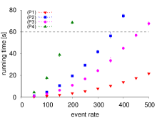
(a) in-order

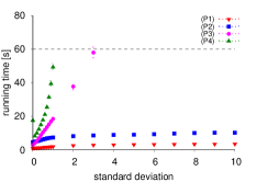
(b) out-of-order

Figure 3: Running times (where each data point shows the mean over five logs together with the minimum and maximum, which are very close to the mean).

In-order Delivery.

In our first setting, messages are received ordered by their timestamps and are never lost. Namely, all events of the log are processed in the order of their timestamps. Figure 3(a) shows the running times of our prototype tool for different event rates. Note that each log spans 60 seconds and a running time below 60 seconds essentially means that the events in the log could have been processed online. The dashed horizontal lines mark this border.

Out-of-order Delivery.

In our second setting, messages can arrive out of order but they are not lost. We control the degree of message arrival disruption as follows. For the events in a generated log file, we choose their arrival times, which provide the order in which the monitor processes them. The arrival time of an event is derived from the event’s timestamp by offsetting it by a random delay with respect to the normal distribution with a mean of 10 time units and a chosen standard deviation. In particular, for an event’s timestamp $\tau$ and for a standard deviation $\sigma>0$, it holds that an arrival time $\tau^{\prime}$ is in the interval $[\tau+10-\sigma,\tau+10+\sigma]$ with probability $0.68$ and in $[\tau+10-2\sigma,\tau+10+2\sigma]$ with probability $0.95$. For the degenerate case $\sigma=0$, the reordered log is identical to the original log. We remark that the mean value does not impact the event reordering because it does not influence the difference between arrival times.

Figure 3(b) shows the prototype’s running times on logs with the fixed event rate 100 for different deviations. For instance, for (P1), the logs are processed in around $1$ second when $\sigma=0$ and in $3.5$ seconds when $\sigma=10$.

Interpretation.

The running times are nonlinear in the event rate for all four formulas. This is expected from Theorem 3.2. The growth is caused by the data values occurring in the events. A log with a higher event rate contains more different data values and the monitor’s state must account for those. As expected, (P1) is the easiest to monitor. It has only one block of freeze quantifiers. Note that (P1)–(P3) have two temporal connectives, where one is the outermost connective $\operatorname{\square}$, which is common to all formulas, whereas (P4) has an additional nesting of temporal connectives. The time window is also larger than in (P1) and (P2).

Also expected, the running times increase when messages are received out of order. Again, (P4) is worst. For (P1) and (P2), however, the growth rate decreases for larger standard deviations. This is because, as the standard deviation increases, all the events within the relevant time window for a given time point arrive at the monitor in an order that is increasingly close to the uniformly random one. The running times thus stabilize. Due to the larger time window, this effect does not take place for (P4). The running times for (P3) increase more rapidly than for (P1) and (P2) because of the data values and the “continuation formula” of the derived unbounded temporal connective $\mathbin{\mathsf{W}}$.

To put the experimental results in perspective, we carried out two additional experiments. First, we conducted similar experiments on formulas with their freeze quantifiers removed and further transformed into propositional formulas, as described in Appendix 0.D.2. We make similar observations in the propositional setting. However, in the propositional setting the running times increase linearly with respect to the event rate and logs are processed several orders of magnitude faster. Overall, one pays a price at runtime for the expressivity gain given by the freeze quantifier. Second, we compared our prototype with the MONPOLY tool [3]. MONPOLY’s specification language is, like MTL^↓, a point-based real-time logic. It is richer than MTL^↓ in that it admits existential and universal quantification over domain elements. However, MONPOLY specifications are syntactically restricted in that temporal future connectives must be bounded (except for the outermost connective $\operatorname{\square}$). Thus, (P3) does not have a counterpart in MONPOLY’s specification language. MONPOLY handles the counterparts of (P1), (P2), and (P4) significantly faster, up to three orders of magnitude. Comparing the performance of both tools should, however, be taken with a grain of salt. First, MONPOLY only handles the restrictive setting where messages must be received in-order. Second, MONPOLY outputs violations for specifications with (bounded) future only after all events in the relevant time window are available, whereas our prototype outputs verdicts promptly. Finally, while MONPOLY is optimized, our prototype is not.

In summary, our experimental evaluation shows that one pays a high price to handle an expressive specification language together with message delays. Nevertheless, our prototype’s performance is sufficient to monitor systems that generate hundreds of events per second, and the prototype can be used as a starting point for a more efficient implementation.

6 Related Work

Runtime verification is a well-established approach for checking at runtime whether a system’s execution fulfills a given specification. Various monitoring algorithms exist, e.g., [2, 10, 18, 5]. They differ in the specifications they can handle (some of the specification languages account for data values) and they make different assumptions on the monitored systems. A commonly made assumption is that a monitor has always complete knowledge about the system behavior up to the current time. Only a few runtime-verification approaches exist that relax this assumption. Note that this assumption is, for instance, not met in distributed systems whose components communicate over unreliable channels.

Closest to our work is the runtime-verification approach by Basin et al. [6]. We use the same system model and our monitoring algorithm extends their monitoring algorithm for the propositional real-time logic MTL. Namely, our algorithm handles the more expressive specification language MTL^↓ and handles data values. Furthermore, we present a semantics for MTL^↓ that is based on three truth values and uses observations instead of timed words. This enables us to cleanly state correctness requirements and establish stronger correctness guarantees for the monitoring algorithm. Basin et al.’s completeness result [6] is limited in that it assumes that all messages are eventually received. Finally, Basin et al. [6] do not evaluate their monitoring algorithm experimentally.

Colombo and Falcone [11] propose a runtime-verification approach, based on formula rewriting, that also allows the monitor to receive messages out of order. Their approach only handles the propositional temporal logic LTL with the three-valued semantics proposed by Bauer et al. [9]. In a nutshell, their approach unfolds temporal connectives as time progresses and special propositions act as placeholders for subformulas. The subsequent assignment of these placeholders to Boolean truth values triggers the reevaluation and simplification of the formula. Their approach only guarantees soundness but not completeness, since the simplification rules used for formula rewriting are incomplete. Finally, its performance with respect to out-of-order messages is not evaluated.

The monitoring approaches by Garg et al. [13] and Basin et al. [4], both targeting the auditing of policies on system logs, also account for knowledge gaps, i.e., logs that may not contain all the actions performed by a system. Both approaches handle rich policy specification languages with first-order quantification and a three-valued semantics. Garg et al.’s approach [13], which is based on formula rewriting, is however, not suited for online use since it does not process logs incrementally. It also only accounts for knowledge gaps in a limited way, namely, the interpretation of a predicate symbol cannot be partially unknown, e.g., for certain time periods. Furthermore, their approach is not complete. Basin et al.’s approach [4], which is based on their prior work [5], can be used online. However, the problem of how to incrementally output verdicts as prior knowledge gaps are resolved is not addressed, and thus it does not deal with out-of-order events. Moreover, the semantics of the specification language handled does not reflect a monitor’s partial view about the system behavior. Instead, it is given for infinite data streams that represent system behavior in the limit.

Several dedicated monitoring approaches for distributed systems have been developed [21, 19, 7]. These approaches only handle less expressive specification languages, namely, the propositional temporal logic LTL or variants thereof. Furthermore, none of them handles message loss or out-of-order delivery of messages, problems that are inherent to such systems because of crashing components and nonuniform delays in message delivery.

A similar extension of MTL with the freeze quantifier is defined by Feng et al. [12]. Their analysis focuses on the computational complexity of the path-checking problem. However, they use a finite trace semantics, which is less suitable for runtime verification. Out-of-order messages are also not considered.

Temporal logics with additional truth values have also been considered in model checking finite-state systems. Closest to our three-valued semantics is the three-valued semantics for LTL by Goidefroid and Piterman [14], which is based on infinite words, not observations (Definition 1). Similar to (T3) of Definition 1, a proposition with the truth value $\bot$ at a position can be refined by $\mathsf{t}$ or $\mathsf{f}$. In contrast, their semantics does not support refinements that add and delete letters, cf. (T1) and (T2) of Definition 1.

7 Conclusion

We have presented a runtime-verification approach to checking real-time specifications given as MTL^↓ formulas. Our approach handles the practically-relevant setting where messages sent to the monitors can be delayed or lost, and it provides soundness and completeness guarantees. Although our experimental evaluation is promising, our approach does not yet scale to monitor systems that generate thousands or even millions of events per second. This requires additional research, including algorithmic optimizations. We plan to do this in future work, as well as to deploy and evaluate our approach in realistic, large-scale case studies.

Acknowledgments.

This work was partly performed within the 5G-ENSURE project (www.5gensure.eu) and received funding from the EU Framework Programme for Research and Innovation Horizon 2020 under grant agreement no. 671562. David Basin acknowledges support from the Swiss National Science Foundation grant Big Data Monitoring (167162).

Appendix 0.A Additional MTL^↓ Details

0.A.1 Standard Boolean Semantics

MTL^↓ with a Boolean semantics has the same syntax as MTL^↓ with a three-valued semantics as defined in Section 3. We use the same syntactic sugar and conventions from Section 3. The Boolean semantics for MTL^↓ is defined over timed words.

To define MTL^↓’s Boolean semantics, we introduce the following notation and terminology. Recall that $D$—the data domain—is a nonempty set of values. Furthermore, let $\Sigma$ be the set of the pairs $(\sigma,\varrho)$, where $\sigma$ is a total function over $P$ with $\sigma(p)\subseteq D^{\iota(p)}$ for $p\in P$ and $\varrho$ is a total function over $R$ with $\varrho(r)\in D$ for $r\in R$. In the following, timed words are always over the alphabet $\Sigma$. Note that the letter at position $i\in\mathbb{N}$ of a timed word (over $\Sigma$) is of the form $(\tau_{i},\sigma_{i},\varrho_{i})$, where $\sigma_{i}$ interprets the predicate symbols at time $\tau_{i}$ and $\varrho_{i}$ determines the values stored in the registers in $R$ at time $\tau_{i}$. As for observations, we call the positions $i\in\mathbb{N}$ of a timed word $w$ the time points of $w$. Furthermore, we call $\tau_{i}$ the timestamp of the time point $i\in\mathbb{N}$.

Remark 1

Observations generalize the notion of a finite prefix of a timed word. Let $w=(\tau_{1},\sigma_{1},\varrho_{1})(\tau_{2},\sigma_{2},\varrho_{2})\dots$ be a timed word. For the prefix of length $n\in\mathbb{N}$ of $w$, we define the word $w_{n}$ as $(\{\tau_{1}\},\sigma_{1},\varrho_{1})\dots(\{\tau_{n}\},\sigma_{n},\varrho_{n})(I,[\,],[\,])$, with $I=\mathbb{Q}_{\geq 0}\setminus\big{(}\bigcup_{1\leq i\leq n}[0,\tau_{i}]\big{)}$. That is, we transform the timestamps of the prefix into singletons and attach a last letter, which can be seen as a placeholder for the remaining letters in $w$. The words $w_{n}$ for $n\in\mathbb{N}$ are observations. Obviously, $w_{0}=([0,\infty),[\,],[\,])$ is an observation. For $n>0$, we obtain $w_{n}$ from $w_{n-1}$ by applying the transformation (T1) with the timestamp $\tau_{n}$ on $w_{n-1}$’s last letter, then applying (T2) to delete the letter with the interval $(\tau_{n-1},\tau_{n})$, and finally applying (T3) on the letter with interval $\{\tau_{n}\}$ to populate it with $\sigma_{n}$ and $\varrho_{n}$.

MTL^↓’s Boolean semantics is defined inductively over the formula structure. In particular, similar to the function $\varphi\mapsto\llbracket{w,i,\nu}\mathrel{|}\joinrel\approx{\varphi}\rrbracket$ defined in Section 3, we define a function $\varphi\mapsto\llbracket{w,i,\nu}\models{p(\bar{x})}\rrbracket\in\mathsf{2}$, for a given timed word $w$, a time point $i\in\mathbb{N}$, and a valuation $\nu:V\nrightarrow D$. Let $w=(\tau_{0},\sigma_{0},\varrho_{0})(\tau_{1},\sigma_{1},\varrho_{1})\dots$.

$$\begin{array}[]{@{}rcl@{}}\llbracket{w,i,\nu}\models{\mathsf{t}}\rrbracket&:=&\mathsf{t}\\[2.84544pt] \llbracket{w,i,\nu}\models{p(\bar{x})}\rrbracket&:=&\begin{cases}\mathsf{t}&\text{if $\nu(\bar{x})\in\sigma_{i}(p)$}\\ \mathsf{f}&\text{otherwise}\end{cases}\\[11.38092pt] \llbracket{w,i,\nu}\models{\mathop{\downarrow^{\!r}}{\!x}\mathbin{\!.}\varphi}\rrbracket&:=&\llbracket{w,i,\nu[x\mapsto\varrho_{i}(r)]}\models{\varphi}\rrbracket\\[2.84544pt] \llbracket{w,i,\nu}\models{\neg\varphi}\rrbracket&:=&\neg\llbracket{w,i,\nu}\models{\varphi}\rrbracket\\[2.84544pt] \llbracket{w,i,\nu}\models{\varphi\vee\psi}\rrbracket&:=&\llbracket{w,i,\nu}\models{\varphi}\rrbracket\vee\llbracket{w,i,\nu}\models{\psi}\rrbracket\\[2.84544pt] \llbracket{w,i,\nu}\models{\varphi\mathbin{\mathsf{U}}_{I}\psi}\rrbracket&:=&\bigvee_{j\in\{\ell\in\mathbb{N}\mathbin{\,|\,}\tau_{\ell}-\tau_{i}\in I\}}\big{(}\llbracket{w,j,\nu}\models{\psi}\rrbracket\wedge\bigwedge_{i\leq k<j}\llbracket{w,k,\nu}\models{\varphi}\rrbracket\big{)}\end{array}$$

Note that we abuse notation here and identify the logic’s constant symbol $\mathsf{t}$ with the Boolean value $\mathsf{t}$, and the connectives $\neg$ and $\vee$ with the corresponding logical operators.

Definition 6

For $\tau\in\mathbb{Q}_{\geq 0}$, a timed word $w$, a valuation $\nu$, and a formula $\varphi$, we define $[{w,\tau,\nu}\models{\varphi}]:=\llbracket{w,j,\nu}\models{\varphi}\rrbracket$, provided that there is some time point $j$ in $w$ with timestamp $\tau$, and $[{w,\tau,\nu}\models{\varphi}]:=\bot$, otherwise.

The following theorem shows that the semantics of MTL^↓ on observations conservatively extends the logic’s semantics on timed words. In particular, if a formula evaluates to a Boolean value for an observation for a given time $\tau\in\mathbb{Q}_{\geq 0}$, it has the same Boolean value on any timed word that refines the observation.

Theorem 0.A.1

Let $\varphi$ be a formula, $\mu$ a partial valuation, $\nu$ a total valuation, $u$ an observation, $v$ a timed word, and $\tau\in\mathbb{Q}_{\geq 0}$. If $u\sqsubseteq v$ and $\mu\sqsubseteq\nu$ then $[{u,\tau,\mu}\mathrel{|}\joinrel\approx{\varphi}]\preceq[{v,\tau,\nu}\models{\varphi}]$.

Proof

Let $(I_{i},\sigma_{i},\varrho_{i})$ and $(\tau_{j},\sigma^{\prime}_{j},\varrho^{\prime}_{j})$, for $i\in\mathit{pos}(u)$ and $j\in\mathbb{N}$ be the letters of $u$ and $v$, respectively. As $u\sqsubseteq v$, we have that there is a function $\pi:\mathbb{N}\to\mathit{pos}(u)$ such that (R1) $\tau_{j}\in I_{\pi(j)}$, (R2) $\sigma_{\pi(j)}\sqsubseteq\sigma^{\prime}_{j}$, and (R3) $\varrho_{\pi(j)}\sqsubseteq\varrho^{\prime}_{j}$, for every $j\in\mathbb{N}$. It is easy to see that $\pi$ is monotonic.

We prove by structural induction on $\varphi$ that for any time point $i^{\prime}\in\mathbb{N}$ and partial valuations $\mu$ and $\nu$ with $\mu\sqsubseteq\nu$, it holds that $\llbracket{u,\pi(i^{\prime}),\mu}\mathrel{|}\joinrel\approx{\varphi}\rrbracket\preceq\llbracket{v,i^{\prime},\nu}\models{\varphi}\rrbracket$. The theorem’s statement easily follows from this property. For the reminder of the proof, we fix an arbitrary time point $i^{\prime}\in\mathbb{N}$ and arbitrary partial valuations $\mu$ and $\nu$ with $\mu\sqsubseteq\nu$. Let $i=\pi(i^{\prime})$.

When $\llbracket{u,i,\mu}\mathrel{|}\joinrel\approx{\varphi}\rrbracket=\bot$ the statement clearly holds. Hence, it suffices to show that $\llbracket{u,i,\mu}\mathrel{|}\joinrel\approx{\varphi}\rrbracket=\llbracket{v,i^{\prime},\nu}\models{\varphi}\rrbracket$, provided that $\llbracket{u,i,\mu}\mathrel{|}\joinrel\approx{\varphi}\rrbracket\in\mathsf{2}$.

Base cases. The case $\varphi=\mathsf{t}$ is trivial. Consider the case $\varphi=p(\bar{x})$, for some $p\in P$. As $\llbracket{u,i,\nu}\mathrel{|}\joinrel\approx{p(\bar{x})}\rrbracket\in\mathsf{2}$, it holds that $\bar{x}\in\operatorname{def}(\nu)$ and $p\in\operatorname{def}(\sigma_{i})$. It follows from the theorem’s premise that $\mu(\bar{x})=\nu(\bar{x})$, and from (R2) that $\sigma_{i}(p)=\sigma^{\prime}_{i^{\prime}}(p)$. Thus $\llbracket{u,i,\nu}\mathrel{|}\joinrel\approx{p(\bar{x})}\rrbracket=\llbracket{v,i^{\prime},\nu}\models{p(\bar{x})}\rrbracket$.

Inductive cases. The cases where $\varphi$ is of the form $\neg\alpha$ or $\alpha\vee\beta$ are straightforward and omitted. The remaining cases are as follows.

First, assume that $\varphi$ is of the form $\mathop{\downarrow^{\!r}}{\!x}\mathbin{\!.}\psi$. Let $\eta=\mu[x\mapsto\varrho_{i}(r)]$ and $\eta^{\prime}=\nu[x\mapsto\varrho^{\prime}_{i^{\prime}}(r)]$. By (R3), we have that if $r\in\operatorname{def}(\varrho_{i})$ then $r\in\operatorname{def}(\varrho^{\prime}_{i^{\prime}})$ and $\varrho_{i}(r)=\varrho^{\prime}_{i^{\prime}}(r)$, and thus $\eta(x)=\eta^{\prime}(x)$. Furthermore, if $r\not\in\operatorname{def}(\varrho_{i})$, then $x\not\in\operatorname{def}(\eta)$. This shows that $\eta\sqsubseteq\eta^{\prime}$. It follows from the induction hypothesis that $\llbracket{u,i,\eta}\mathrel{|}\joinrel\approx{\psi}\rrbracket\preceq\llbracket{v,i^{\prime},\eta^{\prime}}\models{\psi}\rrbracket$. We conclude that $\llbracket{u,i,\mu}\mathrel{|}\joinrel\approx{\varphi}\rrbracket=\llbracket{v,i^{\prime},\nu}\models{\varphi}\rrbracket$.

Finally, assume that $\varphi$ is of the form $\alpha\mathbin{\mathsf{U}}_{I}\beta$. We consider first the case $\llbracket{u,i,\mu}\mathrel{|}\joinrel\approx{\alpha\mathbin{\mathsf{U}}_{I}\beta}\rrbracket=\mathsf{t}$. By definition, there is a $j\geq i$ such that $\mathrm{tp}_{u}(j)=\mathsf{t}$, $\mathrm{tc}_{u,I}(i,j)=\mathsf{t}$, $\llbracket{u,j,\mu}\mathrel{|}\joinrel\approx{\beta}\rrbracket=\mathsf{t}$, and $\mathrm{tp}_{u}(k)\to\llbracket{u,k,\mu}\mathrel{|}\joinrel\approx{\alpha}\rrbracket=\mathsf{t}$, for all $k$ with $i\leq k<j$. As $j$ is a time point in $u$, there is a time point $j^{\prime}$ in $v$ such that $\pi(j^{\prime})=j$. From (R1) we have that $\tau_{j^{\prime}}=\operatorname{ts}_{u}(j)$. As $\mathrm{tc}_{u,I}(i,j)=\mathsf{t}$ and $I_{j}=\{\tau_{j^{\prime}}\}$, we have that $\tau_{j^{\prime}}-\tau\in I$, for all $\tau\in I_{i}$. From (R1), we have that $\tau_{i^{\prime}}\in I_{i}$. Thus $\tau_{j^{\prime}}-\tau_{i^{\prime}}\in I$ (I1). From the induction hypothesis, we have that $\llbracket{u,j,\mu}\mathrel{|}\joinrel\approx{\beta}\rrbracket\preceq\llbracket{v,j^{\prime},\nu}\models{\beta}\rrbracket$. Hence $\llbracket{v,j^{\prime},\nu}\models{\beta}\rrbracket=\mathsf{t}$ (I2). From the induction hypothesis, we also have that $\llbracket{u,\pi(k^{\prime}),\mu}\mathrel{|}\joinrel\approx{\alpha}\rrbracket\preceq\llbracket{v,k^{\prime},\nu}\models{\alpha}\rrbracket$, for any $k^{\prime}\in\mathbb{N}$. Let $k^{\prime}\in\mathbb{N}$ such that $i^{\prime}\leq k^{\prime}<j^{\prime}$, and let $k=\pi(k^{\prime})$. From the monotonicity of $\pi$ we have that $i\leq k\leq j$. Since $j$ is a time point in $u$ we also have that $k<j$. As $\mathrm{tp}_{u}(k)\to\llbracket{u,k,\mu}\mathrel{|}\joinrel\approx{\alpha}\rrbracket=\mathsf{t}$ and $\mathrm{tp}$ is never $\mathsf{f}$ by definition, we have that $\llbracket{u,k,\mu}\mathrel{|}\joinrel\approx{\alpha}\rrbracket=\mathsf{t}$. Then $\llbracket{v,k^{\prime},\mu}\models{\alpha}\rrbracket=\mathsf{t}$ (I3). Summing up, from (I1), (I2), (I3), and as $k^{\prime}$ was chosen arbitrarily, we obtain that $\llbracket{v,i^{\prime},\nu}\models{\alpha\mathbin{\mathsf{U}}_{I}\beta}\rrbracket=\mathsf{t}$.

The case $\llbracket{u,i,\mu}\mathrel{|}\joinrel\approx{\alpha\mathbin{\mathsf{U}}_{I}\beta}\rrbracket=\mathsf{f}$ is as follows. Note that each disjunct in the definition of $\llbracket{u,i,\mu}\mathrel{|}\joinrel\approx{\alpha\mathbin{\mathsf{U}}_{I}\beta}\rrbracket$ is $\mathsf{f}$. We fix an arbitrary $j^{\prime}\geq i^{\prime}$ and let $j=\pi(j^{\prime})$. It holds that $\mathrm{tp}_{u}(j)\wedge\mathrm{tc}_{u,I}(i,j)\wedge\llbracket{u,j,\mu}\mathrel{|}\joinrel\approx{\beta}\rrbracket\wedge\bigwedge_{i\leq k<j}(\mathrm{tp}_{u}(k)\rightarrow\llbracket{u,k,\mu}\mathrel{|}\joinrel\approx{\alpha}\rrbracket)=\mathsf{f}$. Since $\mathrm{tp}_{u}(j)\not=\mathsf{f}$, one of the remaining conjuncts must be $\mathsf{f}$.

1. If $\mathrm{tc}_{u,I}(i,j)=\mathsf{f}$, then $\tau^{\prime}-\tau^{\prime\prime}\not\in I$, for all $\tau^{\prime\prime}\in I_{i}$ and $\tau^{\prime}\in I_{j}$. From (R1), $\tau_{i^{\prime}}\in I_{i}$ and $\tau_{j^{\prime}}\in I_{j}$. It follows that $\tau_{j^{\prime}}-\tau_{i^{\prime}}\not\in I$.

2. If $\llbracket{u,j,\mu}\mathrel{|}\joinrel\approx{\beta}\rrbracket=\mathsf{f}$, then $\llbracket{v,j^{\prime},\nu}\models{\beta}\rrbracket=\mathsf{f}$, by induction hypothesis.

3. If $\mathrm{tp}_{u}(k)\to\llbracket{u,k,\mu}\mathrel{|}\joinrel\approx{\alpha}\rrbracket=\mathsf{f}$, for some $k$ with $i\leq k<j$, then $\mathrm{tp}_{u}(k)=\mathsf{t}$ and $\llbracket{u,k,\mu}\mathrel{|}\joinrel\approx{\alpha}\rrbracket=\mathsf{f}$. It follows as before that there is a $k^{\prime}$ with $i^{\prime}\leq k^{\prime}<j^{\prime}$ such that $\llbracket{v,k^{\prime},\nu}\models{\alpha}\rrbracket=\mathsf{f}$.

We have thus obtained that either $\tau_{i^{\prime}}-\tau_{j^{\prime}}\not\in I$ or one of the conjuncts of $\llbracket{v,j^{\prime},\nu}\models{\beta}\rrbracket\wedge\bigwedge_{i^{\prime}\leq k^{\prime}<j^{\prime}}\llbracket{v,k^{\prime},\nu}\models{\alpha}\rrbracket$ is $\mathsf{f}$. In other words, if $j^{\prime}$ is such that $\tau_{j^{\prime}}-\tau_{i^{\prime}}\in I$, then $\llbracket{v,j^{\prime},\nu}\models{\beta}\rrbracket\wedge\bigwedge_{i^{\prime}\leq k^{\prime}<j^{\prime}}\llbracket{v,k^{\prime},\nu}\models{\alpha}\rrbracket=\mathsf{f}$. As $j^{\prime}$ was chosen arbitrarily, we conclude that $\llbracket{v,i^{\prime},\nu}\models{\alpha\mathbin{\mathsf{U}}_{I}\beta}\rrbracket=\mathsf{f}$. ∎

0.A.2 Correctness Requirements

In this section, we formulate similar monitoring requirements as in Section 4.1, formulating them this time with respect to the Boolean MTL^↓ semantics. We then argue that these requirements are too strong.

For an observation $w$, we define $U_{w}:=\{v\mathbin{\,|\,}v\text{ a timed word with }w\sqsubseteq v\}$. Intuitively, $U_{w}$ contains all the timed words that are compatible with the reported system behavior that a monitor received so far, represented by $w$.

Definition 7

Let $M$ be a monitor, $\varphi$ a formula, and $\bar{w}$ a valid observation sequence.

• $M$ is sound for $\bar{w}$ and $\varphi$ if for all valuations $\nu$ and $i\in\mathbb{N}$, whenever $(\tau,b)\in M(w_{i})$ then $\bigcurlywedge_{v\in U_{w_{i}}}[{v,\tau,\nu}\models{\varphi}]=b$.

• $M$ is complete for $\bar{w}$ and $\varphi$ if for all valuations $\nu$, $i\in\mathbb{N}$, and $\tau\in\mathbb{Q}_{\geq 0}$, whenever $\bigcurlywedge_{v\in U_{w_{i}}}[{v,\tau,\nu}\models{\varphi}]\in\mathsf{2}$ then $(\tau,b)\in\bigcup_{j\leq i}M(w_{j})$, for some $b\in\mathsf{2}$.

We say that $M$ is sound if $M$ is sound for all valid observation sequences $\bar{w}$ and formulas $\varphi$. The definition of $M$ being complete is analogous.

The correctness requirements in Definition 7 are related to the use of a three-valued “runtime-verification” semantics for a specification language, as introduced by Bauer et al. [10] for LTL and adopted by other runtime-verification approaches (e.g. [8]). Intuitively speaking, both a sound and complete monitor and a monitor implementing a three-valued “runtime-verification” semantics output a verdict as soon as the specification has the same Boolean value on every extension of the monitor’s current knowledge. However, Bauer et al. [10] make no distinction between a monitor’s soundness and its completeness. Distinguishing these two requirements separates concerns and this is important, as explained next. Ideally, a monitor is both sound and complete. However, achieving both of these properties can be hard or even impossible for non-trivial specification languages, as we now explain, when relying on the standard Boolean semantics.

Remark 2

For a specification language, having a sound and complete monitor $M$ for a specification language is at least as hard as checking satisfiability for this language. For MTL^↓, a closed formula $\varphi$ is satisfiable iff $(0,\mathsf{f})\not\in M(w_{1})$, assuming that $0$ is always the timestamp of the first time point of a timed word and the observation $w_{1}$ is obtained from the monitor’s initial knowledge $w_{0}$ by (T1) for the timestamp $0$. Note that $w_{0}=([0,\infty),[\,],[\,])$, $U_{w_{0}}$ is the set of all timed words, and $U_{w_{1}}=U_{w_{0}}$. The propositional fragment of MTL^↓ is already undecidable [20]. There are fragments that are decidable but the complexity is usually high. Recall that for LTL, checking satisfiability is already PSPACE-complete.

Some monitoring approaches try to compensate for this complexity burden with a pre-processing step. For instance, the monitoring approach of Bauer et al. [10] translates an LTL formula into an automaton prior to monitoring. The resulting automaton can be directly used for sound and complete monitoring in environments where messages are neither delayed nor lost. However, there are no obvious extensions for handling out-of-order message delivery. Furthermore, not every specification language has such a corresponding automaton model and, for the ones where translations are known, the automaton construction can be very costly. For LTL, the size of the automaton is already in the worst case doubly exponential in the size of the formula [10].

In contrast the correctness requirements from Definition 5 are weaker and achievable. This is due to the three-valued semantics, based on Kleene logic, for MTL^↓ over observations. Furthermore, note that the three-valued semantics for MTL^↓ conservatively extends the standard Boolean semantics, as shown by Theorem 0.A.1.

Theorem 0.A.1 allows us to prove that the completeness requirement from Definition 5 is indeed a weaker notion than completeness requirement from Definition 7, while the soundness requirement from Definition 7 offers the same correctness guarantees as the one from Definition 5.

Theorem 0.A.2

Let $M$ be a monitor. If $M$ is observationally sound, then $M$ is sound. If $M$ is complete, then $M$ is observationally complete.

Proof

First, let $M$ be an observationally sound monitor. Let $\varphi$ be a formula and $\bar{w}$ a valid observation sequence. Furthermore, let $\nu$ be a total valuation, $i\in\mathbb{N}$, $\tau\in\mathbb{Q}_{\geq 0}$, and $b\in\mathsf{2}$ such that $(\tau,b)\in M(i)$. Then, by definition, $[{w_{i},\tau,\nu}\mathrel{|}\joinrel\approx{\varphi}]=b$. Now, let $v\in U_{w_{i}}$. We have that $w_{i}\sqsubseteq v$. Then from Theorem 0.A.1 we have that $[{v,\tau,\nu}\models{\varphi}]=b$. As $v$ was chosen arbitrarily, we get $\bigcurlywedge_{v\in U_{w_{i}}}[{v,\tau,\nu}\models{\varphi}]=b$. Thus $M$ is a sound monitor.

Now, let $M$ be a complete monitor. Let $\varphi$ be a formula and $\bar{w}$ a valid observation sequence. Furthermore, let $\nu$ be a partial valuation, $i\in\mathbb{N}$, $\tau\in\mathbb{Q}_{\geq 0}$ such that $[{w_{i},\tau,\nu}\models{\varphi}]=b^{\prime}$ for some $b^{\prime}\in\mathsf{2}$. Let $\nu^{\prime}$ be a total valuation with $\nu\sqsubseteq\nu^{\prime}$. Also, let $v\in U_{w_{i}}$. Then, as $w_{i}\sqsubseteq v$, from Theorem 0.A.1 we obtain that $[{v,\tau^{\prime},\nu}\models{\varphi}]=b^{\prime}$. As $v$ was chosen arbitrarily, we get $\bigcurlywedge_{v\in U_{w_{i}}}[{v,\tau,\nu^{\prime}}\models{\varphi}]=b^{\prime}$. As $M$ is complete, it follows, by definition, that there is $b\in\mathsf{2}$ and $j\leq i$ such that $(\tau,b)\in M(w_{j})$. Thus $M$ is an observationally complete monitor. ∎

0.A.3 Proof of Theorem 3.1

The following lemma characterizes the relation on observations.

Lemma 1

Let $w$ and $w^{\prime}$ be observations with letters $(I_{i},\sigma_{i},\varrho_{i})$ and respectively $(I^{\prime}_{j},\sigma^{\prime}_{j},\varrho^{\prime}_{j})$, for $i\in\mathit{pos}(w)$ and $j\in\mathit{pos}(w^{\prime})$. If $w\sqsubseteq w^{\prime}$ then there is a monotonic function $\pi:\mathit{pos}(w^{\prime})\rightarrow\mathit{pos}(w)$ with the following properties.

1. $I_{j}^{\prime}\subseteq I_{\pi(j)}$, for all $j\in\mathit{pos}(w^{\prime})$.

2. $\sigma_{\pi(j)}\sqsubseteq\sigma_{j}^{\prime}(p)$, for all $j\in\mathit{pos}(w^{\prime})$ and $p\in P$.

3. $\varrho_{\pi(j)}\sqsubseteq\varrho^{\prime}_{j}$, for all $j\in\mathit{pos}(w^{\prime})$ and $r\in R$.

Proof (sketch)

If $w=w^{\prime}$ then take $\pi$ to be the identity. If $w^{\prime}$ is obtained from $w$ using one of the transformations, that is, if $w\sqsubset w^{\prime}$, then, for each transformation it is easy to construct a function $\pi$ satisfying the stated properties. If $w\sqsubsetneq w^{\prime}$, then there is a sequence $(w_{i})_{0\leq i\leq n}$ of observations, with $n\geq 1$, such that $w=w_{0}\sqsubset w_{1}\sqsubset\dots\sqsubset w_{n}=w^{\prime}$. From the previous observation there is a sequence of functions $\pi_{i}:\mathit{pos}(w_{i})\to\mathit{pos}(w_{i-1})$, with $1\leq i\leq n$, each satisfying the stated properties. Then it is easy to see that their composition $\pi=\pi_{1}\circ\dots\circ\pi_{n}$ also satisfies these properties. ∎

The proof of Theorem 3.1 is similar to that of Theorem 0.A.1 and is thus omitted. We just note that the omitted proof uses properties (R1) to (R3) from Lemma 1, which correspond to the ones given in the proof of Theorem 0.A.1.

0.A.4 Proof of Theorem 3.2

We first show that the problem is PSPACE-hard by reducing the satisfiability problem for quantified Boolean logic (QBL) to it. For simplicity, we assume that MTL^↓ comprises the temporal past-time connectives $\operatorname{\text{\raisebox{-1.1pt}{\begin{turn}{45.0}\scalebox{0.9}{$\blacksquare$}\end{turn}}}}$ (“once”) and $\operatorname{\blacksquare}$ (“historically”), which are the counterparts of $\operatorname{\text{\raisebox{-1.1pt}{\begin{turn}{45.0}\scalebox{0.9}{$\square$}\end{turn}}}}$ and $\operatorname{\square}$. Their semantics is as expected. A slightly more involved reduction without these temporal connectives is possible.

Let $\alpha$ be a closed QBL formula over propositions $p_{1},\dots,p_{n}$. We define the set $P$ of predicate symbols as $\{P_{1},\dots,P_{n}\}$, where each predicate symbol has arity $1$. Moreover, let $R:=\{r\}$ and $D:=\{0,1\}$, and let $w$ be the observation $(\{0\},\sigma,\varrho_{0})(\{1\},\sigma,\varrho_{1})(\{3\},[\,],[\,])((3,\infty),[\,]\,[\,])$, with $\sigma(P_{i})=\{1\}$, for each $i\in\{1,\dots,n\}$, and $\varrho_{i}(r)=i$, for $i\in\{0,1\}$. Finally, we translate the QBL formula $\alpha$ to an MTL^↓ formula $\alpha^{*}$ as follows.

$$\begin{array}[]{@{}r@{\ }lcr@{\ }lcl@{}}p_{i}^{*}&:=P_{i}(x_{i})&&(\neg\beta)^{*}&:=\neg\beta^{*}&&(\beta\vee\gamma)^{*}:=\beta^{*}\vee\gamma^{*}\\ (\exists p_{i}.\,\beta)^{*}&:=\operatorname{\text{\raisebox{-1.1pt}{\begin{turn}{45.0}\scalebox{0.9}{$\blacksquare$}\end{turn}}}}\operatorname{\text{\raisebox{-1.1pt}{\begin{turn}{45.0}\scalebox{0.9}{$\square$}\end{turn}}}}_{[0,1]}\mathop{\downarrow^{\!}}{\!x_{i}}\mathbin{\!.}{\beta^{*}}&&(\forall p_{i}.\,\beta)^{*}&:=\operatorname{\blacksquare}\,\operatorname{\square}_{[0,1]}\mathop{\downarrow^{\!}}{\!x_{i}}\mathbin{\!.}{\beta^{*}}\end{array}$$

It is easy to see that $\alpha$ is satisfiable iff $[{w,0,[\,]}\mathrel{|}\joinrel\approx{\alpha^{*}}]=\mathsf{t}$.

We only sketch the problem’s membership in PSPACE. Note that $w$ is finite. If there is no time point in $w$ with timestamp $\tau$, then $[{w,\tau,\nu}\mathrel{|}\joinrel\approx{\varphi}]=\bot$. Suppose that $i\in\mathit{pos}(w)$ is a time point in $w$ with timestamp $\tau$. A computation of $\varphi$’s truth value at position $i$ can be easily obtained from the inductive definition of the satisfaction relation $\mathrel{|}\joinrel\approx$. This computation can be done in polynomial space when traversing the formula structure depth-first. Note that for a position, a subformula of $\varphi$ might be visited multiple times with possibly different partial valuations.

Appendix 0.B Additional Algorithmic Details

We present in this section the procedures Init, NewTimePoint, PropagateDown, and PropagateUp, which are called from the main procedure. Their pseudo-code is given in the Listings 2 to 5, respectively.

List of listings 2

⬇

procedure Init($\varphi$)

verdicts := $\emptyset$

$J$ := $[0,\infty)$

foreach $\psi\in\mathit{Sub}(\varphi)$ # in a bottom-up manner

case $\psi=p(\bar{x})$: $\Psi^{\psi,J,[\,]}$ := $\psi^{J}$

case $\psi=\neg\alpha$: $\Psi^{\psi,J,[\,]}$ := $\neg\alpha^{J}$

case $\psi=\alpha\lor\beta$: $\Psi^{\psi,J,[\,]}$ := $\alpha^{J}\lor\beta^{J}$

case $\psi=\mathop{\downarrow^{\!}}{\!x}\mathbin{\!.}{\alpha}$: $\Psi^{\psi,J,[\,]}$ := $\alpha^{J}$

case $\psi=\alpha\mathbin{\mathsf{U}}_{I}\beta$:

if $I=[0,\infty)$ then tc := $\mathsf{t}$ else tc := $\mathit{tc}^{J,J}$

$\Psi^{\psi,J,[\,]}$ := tc $\land$ $\bar{\beta}^{J}\land\bar{\bar{\alpha}}^{J}$

foreach $\alpha$ in Atoms($\varphi$) with $\alpha=\mathsf{t}$ do

PropagateUp($\alpha$, $J$, $\mathsf{t}$)

The procedure Init initializes the state of the monitor, which consists of the formulas $\Psi^{\gamma,[0,\infty),[\,]}$, for each subformula $\gamma$ of the monitored formula $\varphi$. These formulas are as defined in Section 4.2.1. The procedure also propagates the Boolean value $\mathsf{t}$ from the atoms $\mathsf{t}$ of $\varphi$.

List of listings 3

⬇

procedure NewTimePoint($\varphi$, $J$, new)

foreach $\psi\in\mathit{Sub}(\varphi)$ # in a top-down manner

foreach $\nu$ with $\Psi^{\psi,J,\nu}$ $\neq$ nil do

foreach $K$ in new do

case $\psi=p(\bar{x})$:

$\Psi^{\psi,K,\nu}$ := Apply($\Psi^{\psi,J,\nu}$, $[\psi^{J}\mapsto\psi^{K}]$)

case $\psi=\neg\alpha$:

$\Psi^{\psi,K,\nu}$ := Apply($\Psi^{\psi,J,\nu}$, $[\alpha^{J}\mapsto\alpha^{K}]$)

case $\psi=\alpha\lor\beta$:

$\Psi^{\psi,K,\nu}$ := Apply($\Psi^{\psi,J,\nu}$, $[\alpha^{J}\mapsto\alpha^{K},\beta^{J}\mapsto\beta^{K}]$)

case $\psi=\mathop{\downarrow^{\!}}{\!x}\mathbin{\!.}\alpha$:

$\Psi^{\psi,K,\nu}$ := Apply($\Psi^{\psi,J,\nu}$, $[\alpha^{J}\mapsto\alpha^{K}]$)

case $\psi=\alpha\mathbin{\mathsf{U}}_{I}\beta$:

$\Psi^{\psi,K,\nu}$ := Apply($\Psi^{\psi,J,\nu}$, $[\mathit{tc}^{H,J}\mapsto\mathit{tc}^{H,K}]_{\mathit{tc}^{H,J}\in\mathit{AP}(\Psi^{\psi,J,\nu})}$)

foreach $\gamma,H,\mu$ with $\psi^{J}\in\mathit{AP}(\Psi^{\gamma,H,\mu})$ and ($\gamma=\psi\mathbin{\mathsf{U}}_{I}\_$ or $\gamma=\psi\mathbin{\mathsf{U}}_{I}\_$)

$\theta$ := RefinementUntil($\gamma$, $H$, $J$, new)

$\Psi^{\gamma,H,\mu}$ := Apply($\Psi^{\gamma,H,\mu}$, $\theta$)

procedure RefinementUntil($\alpha\mathbin{\mathsf{U}}_{I}\beta$, $H$, $J$, new)

anchor, continuation := $\mathsf{f}$, $\mathsf{t}$

for $K$ in new with $K\geq H$ do

if Singleton(K) then cont := $\mathsf{t}$ else $\bar{\bar{\alpha}}^{K}$

anchor := anchor $\lor$ $\bar{\beta}^{K}\land\mathit{tc}^{K,H}\land\mathsf{cont}\land\mathsf{continuation}$

continuation := continuation $\land$ $\bar{\alpha}^{K}$

return $[\mathit{tc}^{J,K}\mapsto\mathsf{t},\bar{\beta}^{J}\mapsto\mathsf{anchor},\bar{\alpha}^{J}\mapsto\mathsf{continuation},\bar{\bar{\alpha}}^{J}\mapsto\mathsf{t}]$

The procedure NewTimePoint transforms formulas $\Psi^{\gamma,K,\nu}$ so that they reflect the interval structure of the new observation, the one obtained after receiving the current message. Recall that, in the pseudo-code, $J$ is the interval that is split at the current iteration and the sequence new consists of those intervals among $J\cap[0,\tau)$, $\{\tau\}$, and $J\cap(\tau,\infty)$ that are not complete. NewTimePoint creates a new formula $\Psi^{\gamma,K,\nu}$ for each $K\in\mathsf{new}$ and each each $\nu$ such that the variable $\Psi^{\gamma,J,\nu}$ is defined. The new formula is obtained by applying a substitution which translates atomic propositions $\alpha^{J}$ into propositional formulas over atomic propositions $\alpha^{K^{\prime}}$ with $K^{\prime}\in\mathsf{new}$. For non-temporal formulas this propositional formula is simply $\alpha^{K}$. That is the substitution is $[\alpha^{J}\mapsto\alpha^{K}]$. For temporal formulas the substitution is obtained in two steps: a first substitution replaces atomic propositions of the form $\mathit{tc}^{H,J}$ with atomic substitutions of the form $\mathit{tc}^{H,K}$, and a second substitution, obtained by calling the procedure RefinementUntil, deals with atomic propositions of the form $\alpha^{J}$.

NewTimePoint also transforms some formulas $\Psi^{\gamma,K,\nu}$ with $K\not\in\mathsf{new}$, that is for intervals $K$ that occur in the letters of the old observation, that is, the one from the previous iteration. It does that for those formulas that have atomic propositions of the form $\alpha^{J}$. Note that then it is necessarily the case that $\gamma$ is a temporal formula. The required substitution is also computed by the RefinementUntil procedure.

The RefinementUntil procedure produces the necessary substitution to update the atomic propositions $\bar{\alpha}^{J}$, $\bar{\bar{\alpha}}^{J}$, and $\bar{\beta}^{J}$ that may occur in formulas $\Psi^{\gamma,H,\nu}$ for some interval $H$ of the new observation, where $\gamma=\alpha\mathbin{\mathsf{U}}_{I}\beta$. (Note that before calling RefinementUntil the new formulas $\Psi^{\gamma,K,\nu}$ with $K\in\mathsf{new}$ have already been created.) The substitution of the proposition $\bar{\alpha}^{J}$ is straightforward. Namely, we replace $\bar{\alpha}^{J}$ by the conjunction $\bigwedge_{K\in\mathsf{new},K\geq H}\bar{\alpha}^{K}$. Next, the atomic propositions $\mathit{tc}^{J,K}$ and $\bar{\bar{\alpha}}^{J}$ are discarded: they appeared in $\Psi^{\gamma,H,\nu}$ as conjuncts and thus replacing them by $\mathsf{t}$ effectively discards them. The substitution of $\bar{\beta}^{J}$ is more involved. We illustrate it with an example. Suppose that $\mathsf{new}=(K_{1},K_{2},K_{3})$ and that $H\leq K_{1}$. Note that $K_{2}$ is a singleton. In this case, $\bar{\beta}^{J}$ is substituted by the following formula.

$$\bar{\beta}^{K_{1}}\land\mathit{tc}^{K_{1},H}\land\bar{\bar{\alpha}}^{K_{1}}\ \lor$$

$$\bar{\beta}^{K_{2}}\land\mathit{tc}^{K_{2},H}\land\bar{\alpha}^{K_{1}}\ \lor$$

$$\bar{\beta}^{K_{3}}\land\mathit{tc}^{K_{3},H}\land\bar{\bar{\alpha}}^{K_{3}}\land\bar{\alpha}^{K_{2}}\land\bar{\alpha}^{K_{1}}$$

The application of the computed substitution is performed by the procedure Apply given in Listing 5. Apply actually does more than just applying the substitution given as an argument. First, it also simplifies the resulting formula. The actual application and the simplification are performed by procedure Substitute, which is as expected and thus not detailed further. Second, Apply checks whether the resulting formula is a Boolean constant. If this is the case, then propagation is initiated by calling the PropagateUp procedure.

Note that if $\Psi^{\gamma,J,\nu}$ is already a Boolean constant that has not yet been propagated, because for instance the $\gamma=\bar{\beta}$ and the constant is $\mathsf{t}$, then, since Apply tries again to propagate it, this Boolean value will actually be propagated for the new interval $\{\tau\}$, as it is a singleton and thus corresponds to a time point.

List of listings 4

⬇

procedure PropagateDown($\psi$, $J$, $x$, $d$)

foreach $\nu$ with $\Psi^{\psi,J,\nu}$ $\neq$ nil

$\Psi^{\psi,J,\nu[x\mapsto d]}$ := $\Psi^{\psi,J,\nu}$

if $\psi$ $\not\in$ Atoms($\varphi$) then

foreach $\alpha^{K}\in\mathit{AP}(\Psi^{\psi,J,\nu})$

PropagateDown($\alpha$, $K$, $x$, $d$)

The pseudo-code of the procedures PropagateDown and PropagateUp is straightforward in that it implements downward and upward propagation exactly as described in Section 4.2.2.

List of listings 5

⬇

procedure Apply($\Psi^{\psi,J,\nu}$, $\theta$)

$f$ := Substitute($\Psi^{\psi,J,\nu}$, $\theta$)

if $f\in\mathsf{2}$ then PropagateUp($\psi$, $J$, $\nu$, $f$)

return $f$

procedure PropagateUp($\psi$, $J$, $b$)

$\gamma$ := Parent($\psi$)

if $\gamma$ = nil then

if Singleton($J$) then verdicts := verdicts $\cup$ $\{(\mathsf{Timestamp}(J),b)\}$

else if CanPropagateUp($\psi$, $J$, $b$)

$\theta$ := [$\psi^{J}\mapsto b$]

foreach $K,\mu$ with $\psi^{J}\in\mathit{AP}(\Psi^{\gamma,K,\mu})$

$\Psi^{\gamma,K,\mu}$ := Apply($\Psi^{\gamma,K,\mu}$, $\theta$)

procedure CanPropagateUp($\psi$, $J$, $b$)

$\gamma$ := Parent($\psi$)

case $\gamma$ = nil or $\gamma\neq\_\mathbin{\mathsf{U}}_{I}\_$: return $\mathsf{t}$

case $\gamma$ = $\_\mathbin{\mathsf{U}}_{I}\psi$: return (Singleton($J$) or not $b$)

case $\gamma$ = $\psi\mathbin{\mathsf{U}}_{I}\_$: return (Singleton($J$) or $b$)

Appendix 0.C Soundness and Completeness Proof

In this section, we will consider many substitutions from atomic propositions to propositional formulas. Given such a substitution $\theta$ and a propositional formula $\psi$, we denote by $\theta(\psi)$ and $\psi\theta$ the formula obtained by replacing in $\psi$ the atomic propositions $p$ that occur in both $\psi$ and in $\operatorname{def}(\theta_{i})$ by $\theta_{i}(p)$.

0.C.1 Overview

Let $\bar{w}$ be valid observation sequence and let $\varphi$ be the monitored formula. We assume that $\varphi$ is not an atomic formula. We let $(J^{i}_{j},\sigma^{i}_{j},\varrho^{i}_{j})$ be the $j$th letter of $w_{i}$. We drop the superscript $i$ if it is clear from the context. Also, given an interval $J$ in $w_{i}$, we denote by $\hat{J}$ the index $j\in\mathit{pos}(w_{i})$ such that $J_{j}=J$, assuming that the iteration $i$ is clear from the context.

We first state a lemma from which correctness follows, and only later prove the lemma. We recall that $\Psi_{i}^{\psi,J,\nu}$ denotes the the value of the variable $\Psi^{\psi,J,\nu}$ from the pseudo-code at the end of iteration $i$.

Lemma 2

For any $i\in\mathbb{N}$, $j\in\mathit{pos}(w_{i})$, and $b\in\mathsf{2}$, we have that

$$\theta_{i}^{[\,]}(\Phi_{i}^{\varphi,J})=b\quad\text{iff}\quad\Psi_{i}^{\varphi,J,[\,]}=b,$$

where $J$ is the interval of the $j$th letter of $w_{i}$.

We show next how observational soundness and completeness follow from this lemma. We first note that for any iteration $i\in\mathbb{N}$, the variable $\Psi^{\psi,J,\nu}$ is defined at the end of iteration $i$ for some $\nu$ if and only if $\psi$ is a subformula of $\varphi$ and $J$ is an interval in $w_{i}$. Next, we note that the global variable verdicts is only updated in the execution of PropagateUp($\psi$, $J$, $b$) when $\psi=\varphi$ and $J$ is a singleton. Furthermore, by analyzing where it is called from, we see that all calls are preceded by setting $\Psi^{\psi,J,\nu}$ to $b$. Moreover, $\nu$ has to be $[\,]$ because for any defined variable $\Psi^{\psi,J,\nu}$ with $\nu\neq[\,]$ we have that $\psi\neq\varphi$. Indeed, $\Psi^{\psi,J,\nu}$ is only used with a “new” $\nu$ in PropagateDown and this procedure is never called for $\psi=\varphi$. We thus obtain that if some tuple $(\tau,b)$ is added to verdicts then $\Psi^{\varphi,\{\tau\},[\,]}=b$.

Observational soundness follows directly from the lemma, the above stated properties of $\theta_{i}^{\nu}$ and $\Phi_{i}$, and the observations made in the previous paragraph. Note that, since $\varphi$ is closed, then $\llbracket{w_{i},j,\nu}\mathrel{|}\joinrel\approx{\varphi}\rrbracket=\llbracket{w_{i},j,[\,]}\mathrel{|}\joinrel\approx{\varphi}\rrbracket$, for any partial valuation $\nu$.

Consider now completeness. Say that $\llbracket{w_{i},j,\nu}\mathrel{|}\joinrel\approx{\varphi}\rrbracket=b\in\mathsf{2}$ and $j$ is a time point with timestamp $\tau$. Let $J=\{\tau\}$. Then $\llbracket{w_{i},j,[\,]}\mathrel{|}\joinrel\approx{\varphi}\rrbracket=b$ and thus $\theta_{i}^{[\,]}(\Phi_{i}^{\varphi,J})=b$. By the lemma, we have that $\Psi_{i}^{\varphi,J,[\,]}=b$. Then there is an iteration $i^{\prime}\leq i$ when $\Psi_{i^{\prime}}^{\varphi,J^{\prime},[\,]}$ has been set to $b$, where $J^{\prime}$ is the interval in $w_{i^{\prime}}$ from which $J$ originates. Let $i^{\prime\prime}$ be the first iteration when $J$ is a letter of $w_{k}$ for some $k$. At this iteration $\Psi_{i^{\prime\prime}}^{\varphi,J,[\,]}$ is set to $\Psi_{i^{\prime}}^{\varphi,J^{\prime},[\,]}$ (see the NewTimePoint procedure). Clearly $i^{\prime}\leq i^{\prime\prime}\leq i$. The setting of $\Psi_{i^{\prime\prime}}^{\psi,J,[\,]}$ to a new value is preceded by a call to Apply, and since this new value is a Boolean value, Apply calls PropagateUp which adds $(\tau,b)$ to verdicts.

0.C.2 The Key Lemma

We state next the key lemma of the proof, from which Lemma 2 follows. In order to state this more general lemma, we first introduce some additional notation.

0.C.2.1 Additional Notation.

Given an $i\in\mathbb{N}$, a subformula $\psi$ of $\varphi$, and a $j\in\mathit{pos}(w_{i})$, we define inductively the set $\mathit{Val}_{i}(\psi,j)$ of relevant valuations for $\psi$ at iteration $i$ and position $j$. For $i=0$, we set $\mathit{Val}_{i}(\psi,0):=\{[\,]\}$, for any subformula $\psi$ of $\varphi$, and for $i>0$ we let

$$\mathit{Val}^{\prime}_{i}(\psi,j) :=\left\{\begin{array}[]{l@{\quad}l}\{[\,]\}&\text{if $\psi=\varphi$},\\ \mathit{Val}_{i}(\gamma,j)&\text{if $\gamma=\neg\psi$, $\gamma=\psi\lor\psi^{\prime}$, or $\gamma=\psi^{\prime}\lor\psi$},\\ \{\nu[x\mapsto\varrho^{i}_{j}(r)]\mathbin{\,|\,}\nu\in\mathit{Val}_{i}(\gamma,j)\}&\text{if $\gamma=\mathop{\downarrow^{\!x}}{\!r}\mathbin{\!.}{\psi}$}\\ \cup_{h\in A}\mathit{Val}_{i}(\gamma,h)&\text{if $\gamma=\psi\mathbin{\mathsf{U}}_{I}\psi^{\prime}$}\\ \cup_{k\in B}\mathit{Val}_{i}(\gamma,k)&\text{if $\gamma=\psi^{\prime}\mathbin{\mathsf{U}}_{I}\psi$}\end{array}\right.$$

and

$$\mathit{Val}_{i}(\psi,j) :=\{\nu\in\mathit{Val}^{\prime}_{i}(\psi,j)\mathbin{\,|\,}\llbracket{w_{i},j,\nu}\mathrel{|}\joinrel\approx{\psi}\rrbracket\not\in\mathsf{2}\},$$

where $\gamma$ is the “parent” of $\psi$ (i.e. the subformula of $\varphi$ that has $\psi$ as a direct subformula) and

$$A:= \;\{h\in\mathbb{N}\mathbin{\,|\,}k<h\leq j\text{ where $k\in\mathbb{N}$ is such that $k\leq j$ and $\mathrm{tc}_{w_{i},I}(j,k)\neq\mathsf{f}$}\},$$

$$B:= \;\{k\in\mathbb{N}\mathbin{\,|\,}k\leq j\text{ and $\mathrm{tc}_{w_{i},I}(j,k)\neq\mathsf{f}$}\}.$$

We denote by $\mathit{AP}_{i}$ the set of the atomic propositions used by the formulas $\Phi_{i}^{\gamma,J}$. We let $\mkern 1.5mu\overline{\mkern-4.5mu\mathit{AP}\mkern-1.5mu}\mkern 1.5mu_{i}$ be the set of atomic propositions obtained from $\mathit{AP}_{i}$ be removing the atomic propositions of the form $\mathit{tp}^{J}$ and replacing atomic propositions of the form $\beta^{J}$ and $\alpha^{J}$ where $\alpha\mathbin{\mathsf{U}}_{I}\beta$ is an subformula of $\varphi$ for some $I$, by the atomic propositions $\bar{\beta}^{J}$ and respectively $\bar{\alpha}^{J}$ and $\bar{\bar{\alpha}}^{J}$. Note that $\mkern 1.5mu\overline{\mkern-4.5mu\mathit{AP}\mkern-1.5mu}\mkern 1.5mu_{i}$ represents the set of atomic propositions of the formulas $\Psi_{i}^{\gamma,J,\nu}$ from the pseudo-code.

We also let $\hat{\delta}_{i}^{\nu}$ be the following substitution:

$$\hat{\delta}_{i}^{\nu}(\bar{\beta}^{J}):= \left\{\begin{array}[]{l@{\quad}l}\mathit{tp}^{J}\land\beta^{J}&\text{if $J$ not a singleton and $\Psi_{i}^{\beta,J,\nu}\notin\mathsf{2}$}\\ \mathit{tp}^{J}&\text{if $J$ not a singleton and $\Psi_{i}^{\beta,J,\nu}=\mathsf{t}$}\\ \beta^{J}&\text{if $J$ is a singleton and $\Psi_{i}^{\beta,J,\nu}\notin\mathsf{2}$}\\ \text{undefined}&\text{otherwise}\end{array}\right.$$

$$\hat{\delta}_{i}^{\nu}(\bar{\alpha}^{J}):= \left\{\begin{array}[]{l@{\quad}l}\mathit{tp}^{J}\to\alpha^{J}&\text{if $J$ not a singleton and $\Psi_{i}^{\alpha,J,\nu}\notin\mathsf{2}$}\\ \neg\mathit{tp}^{J}&\text{if $J$ not a singleton and $\Psi_{i}^{\alpha,J,\nu}=\mathsf{f}$}\\ \alpha^{J}&\text{if $J$ is a singleton and $\Psi_{i}^{\alpha,J,\nu}\notin\mathsf{2}$}\\ \text{undefined}&\text{otherwise}\end{array}\right.$$

$$\hat{\delta}_{i}^{\nu}(\bar{\bar{\alpha}}^{J}):= \left\{\begin{array}[]{l@{\quad}l}\mathit{tp}^{J}\lor\alpha^{J}&\text{if $J$ not a singleton and $\Psi_{i}^{\alpha,J,\nu}\notin\mathsf{2}$}\\ \mathit{tp}^{J}&\text{if $J$ not a singleton and $\Psi_{i}^{\alpha,J,\nu}=\mathsf{f}$}\\ \alpha^{J}&\text{if $J$ is a singleton and $\Psi_{i}^{\alpha,J,\nu}\notin\mathsf{2}$}\\ \text{undefined}&\text{otherwise}\end{array}\right.$$

Note that, for instance when $J$ is a singleton and $\Psi_{i}^{\alpha,J,\nu}=\mathsf{t}$, there is no need to define $\hat{\delta}_{i}^{\nu}(\bar{\alpha}^{J})$, because in this case $\bar{\alpha}^{J}$ is not an atomic proposition of $\Psi_{i}^{\alpha\mathbin{\mathsf{U}}_{I}\beta,K,\nu}$: that atomic proposition has already been instantiated.

0.C.2.2 The Lemma and its Proof.

The following key lemma states the main invariant of the monitoring algorithm.

Lemma 3

For any non-atomic subformula $\psi$ of $\varphi$, $i\in\mathbb{N}$, $j\in\mathit{pos}(w_{i})$, partial valuation $\nu\in\mathit{Val}_{i}(\psi,j)$, we have that

$$\theta_{i}^{\mu}(\Phi_{i}^{\psi,J})\equiv\hat{\delta}_{i}^{\mu}(\Psi_{i}^{\psi,J,\nu}),$$

where $J$ is the interval of the $j$th letter of $w_{i}$ and $\mu=\nu[x\mapsto\varrho^{i}_{j}(r)]$ if $\psi=\mathop{\downarrow^{\!r}}{\!x}\mathbin{\!.}{\alpha}$ and $\mu=\nu$ otherwise.

We first note that Lemma 2 follows easily from Lemma 3. Indeed, we just need to show that, $\hat{\delta}_{i}^{\mu}(\Psi_{i}^{\varphi,J,[\,]})=b$ iff $\Psi_{i}^{\varphi,J,[\,]}=b$, for any $b\in\mathsf{2}$ where $\mu$ is an in the lemma statement. The right to left direction is trivial, while the left to right direction also follows easily: if $\Psi_{i}^{\varphi,J,[\,]}\notin\mathsf{2}$ then it contains at least an atomic proposition, and then $\hat{\delta}_{i}^{[\,]}(\Psi_{i}^{\varphi,J,[\,]})$ also contains an atomic proposition, by the definition of $\hat{\delta}_{i}^{\mu}$, and thus $\hat{\delta}_{i}^{\mu}(\Psi_{i}^{\varphi,J,[\,]})\notin\mathsf{2}$ too.

We devote the rest of this section to the proof of Lemma 3. We start with an assumption and continue with a series of definitions.

We assume in the pseudo-code that formula rewriting (that is, applying substitutions) and propagations are separated into two distinct phases. Note that this can be easily achieved by postponing propagations, that is, by storing all tuples $(\varphi,J,f)$ with $f\in\mathsf{2}$ that occur during the execution of Apply, and by performing the corresponding propagations at the end of the NewTimePoint procedure. We choose not to present this two-phase version of the pseudo-code in order to keep the pseudo-code more compact.

Let $\mathsf{new}_{i}$ be the value of new at iteration $i>0$. Given an interval $J\in\mathsf{new}_{i}$, we let $\zeta^{J}_{i}$ be the substitution computed by the pseudo-code at some iteration $i>0$ during the formula rewriting phase. Note that there is no formula rewriting phase at iteration $i=0$. For $i>0$, for instance when $\alpha$ is such that its parent is $\psi=\neg\alpha$, we have that $\zeta^{J}_{i}(\alpha^{J^{\prime}})=\alpha^{J}$ when $J$ is a new interval in $w_{i}$ obtained by splitting the interval $J^{\prime}$ in $w_{i-1}$.

We let $\bar{\xi}_{i}^{\nu}$ be the substitution computed by the pseudo-code at iteration $i$ during the propagation phase for the partial valuation $\nu$. Formally, $\bar{\xi}_{i}^{\nu}$ is a partial valuation over $\mkern 1.5mu\overline{\mkern-4.5mu\mathit{AP}\mkern-1.5mu}\mkern 1.5mu_{i}$ defined as follows:

$$\xi_{i}^{\nu}(p(\bar{x})^{J}) :=\hskip 8.00003pt\mathsf{t}\qquad\text{if $\bar{x}\in\operatorname{def}(\varphi)$, $p\in\operatorname{def}(\sigma)$, and $\nu(\bar{x})\in\sigma(p)$},$$

$$\xi_{i}^{\nu}(p(\bar{x})^{J}) :=\hskip 8.00003pt\mathsf{f}\qquad\text{if $\bar{x}\in\operatorname{def}(\varphi)$, $p\in\operatorname{def}(\sigma)$, and $\nu(\bar{x})\not\in\sigma(p)$},$$

$$\bar{\xi}_{i}^{\nu}(\gamma^{J}) :=\hskip 8.00003ptb\qquad\text{if $\gamma$ is non-atomic and $\Psi_{i}^{\gamma,J,\nu}=b\in\mathsf{2}$},$$

$$\bar{\xi}_{i}^{\nu}(\bar{\beta}^{J}) :=\left\{\begin{array}[]{l@{\qquad}l}\mathsf{t}&\text{if $J$ is a singleton and $\Psi_{i}^{\beta,J,\nu}=\mathsf{t}$},\\ \mathsf{f}&\text{if $\Psi_{i}^{\beta,J,\nu}=\mathsf{f}$},\end{array}\right.$$

$$\bar{\xi}_{i}^{\nu}(\bar{\alpha}^{J}):=\bar{\xi}_{i}^{\nu}(\bar{\bar{\alpha}}^{J}) :=\left\{\begin{array}[]{l@{\qquad}l}\mathsf{t}&\text{if $\Psi_{i}^{\alpha,J,\nu}=\mathsf{t}$},\\ \mathsf{f}&\text{if $J$ is a singleton and $\Psi_{i}^{\alpha,J,\nu}=\mathsf{f}$},\end{array}\right.$$

$$\bar{\xi}_{i}^{\nu}(\mathit{tc}_{\alpha\mathbin{\mathsf{U}}_{I}\beta}^{K,J}) :=\left\{\begin{array}[]{l@{\qquad}l}\mathsf{t}&\text{if $(K-J)\subseteq I$},\\ \mathsf{f}&\text{if $(K-J)\cap I=\emptyset$}.\end{array}\right.$$

For any $i>0$, subformula $\psi$ of $\varphi$, and interval $J$ in $w_{i}$, we have

$$\Psi_{i}^{\psi,J,\nu}:=\bar{\xi}_{i}^{\mu}(\zeta^{J}_{i}(\Psi_{i-1}^{\psi,J^{\prime},\nu})),$$ (1)

where $J^{\prime}$ is the interval in $w_{i-1}$ from which $J$ originates and $\mu=\nu[x\mapsto\varrho^{i}_{j}(r)]$ if $\psi=\mathop{\downarrow^{\!r}}{\!x}\mathbin{\!.}{\alpha}$ and $\mu=\nu$ otherwise.

We define next the substitution $\xi_{i}^{\nu}$ over $\mathit{AP}_{i}$ and which is a variant of $\bar{\xi}_{i}^{\nu}$:

$$\xi_{i}^{\nu}(\gamma^{J}) :=\bar{\xi}_{i}^{\nu}(\gamma^{J})\quad\text{if $\gamma\in\mathit{Sub}(\varphi)$},$$

$$\xi_{i}^{\nu}(\mathit{tp}^{J}) :=\mathsf{t}\hskip 35.00005pt\text{if $J$ is a singleton},$$

$$\xi_{i}^{\nu}(\mathit{tc}_{\psi}^{K,J}) :=\bar{\xi}_{i}^{\nu}(\mathit{tc}_{\psi}^{K,J}).$$

We also let $\bar{\delta}_{i}$ be the following substitution:

$$\bar{\delta}_{i}(\bar{\beta}^{J}) :=\mathit{tp}^{J}\land\beta^{J},$$

$$\bar{\delta}_{i}(\bar{\alpha}^{J}) :=\mathit{tp}^{J}\to\alpha^{J},$$

$$\bar{\delta}_{i}(\bar{\bar{\alpha}}^{J}) :=\mathit{tp}^{J}\lor\alpha^{J}.$$

Note that we do not have that $\hat{\delta}_{i}^{\nu}=\xi_{i}^{\nu}\circ\bar{\delta}_{i}$. Indeed, if $\Psi_{i}^{\beta,J,\nu}=\mathsf{f}$ then $\bar{\beta}^{J}\,\hat{\delta}_{i}^{\nu}=\bar{\beta}^{J}$, while $\bar{\beta}^{J}\,\bar{\delta}_{i}\,\xi_{i}^{\nu}=\mathsf{f}$. However, as we will prove later, we have that $\hat{\delta}_{i}^{\nu}\circ\bar{\xi}_{i}^{\nu}=\xi_{i}^{\nu}\circ\bar{\delta}_{i}$.

For $i>0$ and partial valuation $\nu$, we define the substitution $\theta_{i-1,i}^{\nu}$ such that it behaves as $\theta_{i-1}^{\nu}$, but it acts however on the atomic propositions of formulas $\Phi_{i}^{\gamma,J,\nu}$. In other words, in contrast to $\theta_{i}^{\nu}$, it does not take into account the new interpretations received at iteration $i$. Formally, $\theta_{i-1,i}^{\nu}$ is a partial function over $\mathit{AP}_{i}$ defined by

$$\theta_{i-1,i}^{\nu}(\alpha^{J}):= \ \theta_{i-1}^{\nu}(\alpha^{J^{\prime}})$$

$$\theta_{i-1,i}^{\nu}(\mathit{tp}^{J}):= \ \theta_{i-1}^{\nu}(\mathit{tp}^{J^{\prime}})$$

$$\theta_{i-1,i}^{\nu}(\mathit{tc}^{H,K}):= \ \theta_{i-1}^{\nu}(\mathit{tc}^{H^{\prime},K^{\prime}}),$$

where $J^{\prime}$, $H^{\prime}$, and $K^{\prime}$ are the intervals in $w_{i-1}$ from which the intervals $J$, $H$, and respectively $K$ originate.

Finally, we let $\theta_{i,\Delta}$ be the substitution defined over $\mathit{AP}_{i}$ by

$$\begin{array}[]{rl@{\quad}l}\theta_{i,\Delta}^{\nu}(\alpha^{J}):=&\theta_{i}^{\nu}(\alpha^{J})&\text{if $i=0$ or $\theta_{i-1}^{\nu}$ is undefined on $\alpha^{J^{\prime}}$,}\\ \theta_{i,\Delta}^{\nu}(\mathit{tp}^{J}):=&\theta_{i}^{\nu}(\mathit{tp}^{J})&\text{if $i=0$ or $\theta_{i-1}^{\nu}$ is undefined on $\mathit{tp}^{J^{\prime}}$,}\\ \theta_{i,\Delta}^{\nu}(\mathit{tc}^{H,K}):=&\theta_{i}^{\nu}(\mathit{tc}^{H,K})&\text{if $i=0$ or $\theta_{i-1}^{\nu}$ is undefined on $\mathit{tc}^{H^{\prime},K^{\prime}}$,}\end{array}$$

where, when $i>0$, $J^{\prime}$, $H^{\prime}$, and $K^{\prime}$ are the intervals in $w_{i-1}$ from which the intervals $J$, $H$, and respectively $K$ originate.

Clearly, we have that

$$\theta_{i}^{\nu} =\theta_{i-1,i}^{\nu}\,\theta_{i,\Delta}^{\nu},\quad\text{for $i>0$},$$ (2)

$$\theta_{0}^{\nu} =\theta_{0,\Delta}^{\nu}.$$ (3)

The following easy to prove equivalence will also be useful:

$$\Phi_{i}^{\psi,J}\theta_{i}^{\mu}=b\quad\text{iff}\quad\psi^{J}\theta_{i}^{\nu}=b,$$ (4)

for any formula $\psi$ that is a subformula of $\varphi$ and any $b\in\mathsf{2}$, and where $\mu=\nu[x\mapsto\varrho^{i}_{j}(r)]$ if $\psi=\mathop{\downarrow^{\!r}}{\!x}\mathbin{\!.}{\alpha}$ and $\mu=\nu$ otherwise.

We summarize in Table 2 all substitutions used in the proof together with their informal meaning.

Table 2: Summary of substitutions used in the proof.

notation	domain	intuition
$\theta_{i}^{\nu}$	$\mathit{AP}_{i}$	$\gamma^{J}\mapsto\llbracket{w_{i},\hat{J},\nu}\mathrel{|}\joinrel\approx{\gamma}\rrbracket$ if in $\mathsf{2}$
$\theta_{i-1,i}^{\nu}$	$\mathit{AP}_{i}$	”extension” of $\theta_{i-1}^{\nu}$ from $A_{i-1}$ to $\mathit{AP}_{i}$
$\theta_{i,\Delta}^{\nu}$	$\mathit{AP}_{i}$	a substitution such that $\theta_{i}^{\nu}=\theta_{i-1,i}^{\nu}\,\theta_{i,\Delta}^{\nu}$
$\bar{\zeta}_{i}^{J}$	$\mkern 1.5mu\overline{\mkern-4.5mu\mathit{AP}\mkern-1.5mu}\mkern 1.5mu_{i-1}$	the substitution of the rewriting phase
$\zeta_{i}^{J}$	$\mathit{AP}_{i-1}$	variant of $\bar{\zeta}_{i}^{J}$ over $\mathit{AP}_{i-1}$ such that $\bar{\zeta}^{J}_{i}\,\bar{\delta}_{i}\equiv\bar{\delta}_{i-1}\,\zeta^{J}_{i}$
$\bar{\xi}_{i}^{\nu}$	$\mkern 1.5mu\overline{\mkern-4.5mu\mathit{AP}\mkern-1.5mu}\mkern 1.5mu_{i}$	the substitution of the propagation phase
$\xi_{i}^{\nu}$	$\mathit{AP}_{i}$	$\gamma^{J}\mapsto\Psi_{i}^{\gamma,J,\nu}$ if in $\mathsf{2}$
$\bar{\delta}_{i}$	$\mkern 1.5mu\overline{\mkern-4.5mu\mathit{AP}\mkern-1.5mu}\mkern 1.5mu_{i}$	e.g. $\bar{\beta}^{J}\mapsto\mathit{tp}^{J}\land\beta^{J}$
$\hat{\delta}_{i}^{\nu}$	$\mkern 1.5mu\overline{\mkern-4.5mu\mathit{AP}\mkern-1.5mu}\mkern 1.5mu_{i}$	variant of $\bar{\delta}_{i}$, taking propagations into account

In the remaining proof, we will use equivalences between substitutions, with the following meaning. Given two substitutions $\theta$ and $\theta^{\prime}$ from atomic propositions to propositional formulas, we write that $\theta\equiv\theta^{\prime}$ iff $\operatorname{def}(\theta)=\operatorname{def}(\theta^{\prime})$ and $p\theta\equiv p\theta^{\prime}$, for any $p\in\operatorname{def}(\theta)$.

Next, we prove Lemma 3 by nested induction, the outer induction being on the iteration $i$ and the inner induction being a structural induction on $\psi$.

Outer base case: $i=0$. We have a single letter in $w_{0}$ with the interval $J=[0,\infty)$. Let $\bar{\Psi}_{0}^{\psi,J,[\,]}$ be the value of $\Psi^{\psi,J,[\,]}$ at the point of execution of the Init procedure (thus at iteration $0$) between the two foreach loops, that is, before propagation of the $\mathsf{t}$ atoms. We thus have that

$$\Psi_{0}^{\gamma,J,[\,]}=\bar{\Psi}_{0}^{\gamma,J,[\,]}\,\bar{\xi}_{0}^{[\,]}.$$ (5)

We also have that

$$\bar{\Psi}_{0}^{\gamma,J,[\,]}\bar{\delta}_{0}\equiv\Phi_{0}^{\gamma,J}.$$ (6)

This is easy to check by inspecting the Init procedure. For instance, for formulas $\gamma=\alpha\mathbin{\mathsf{U}}_{I}\beta$, we have that $\bar{\Psi}_{0}^{\gamma,J}=\mathit{tc}^{J,J}\land\bar{\beta}^{J}\land\bar{\bar{\alpha}}^{J}$ and thus

$$\bar{\Psi}_{0}^{\gamma,J}\bar{\delta}_{0}=\mathit{tc}^{J,J}\land(\mathit{tp}^{J}\land\beta^{J})\land(\mathit{tp}^{J}\lor\alpha^{J})\equiv\mathit{tp}^{J}\land\mathit{tc}^{J,J}\land\beta^{J}=\Phi_{0}^{\gamma,J}.$$

This case then follows from the following sequence of equivalences:

$$\begin{array}[]{r@{\quad}l}{\color[rgb]{0,0,1}\Psi_{0}^{\gamma,J,[\,]}}\,\hat{\delta}_{0}^{[\,]}\equiv&\text{\small[by (\ref{eq:Psi0}): $\Psi_{0}^{\gamma,J,[\,]}=\bar{\Psi}_{0}^{\gamma,J,[\,]}\,\bar{\xi}_{0}$]}\\[2.15277pt] \bar{\Psi}_{0}^{\gamma,J}\,{\color[rgb]{0,0,1}\bar{\xi}_{0}^{[\,]}\,\hat{\delta}_{0}}\equiv&\text{\small[by (\ref{eq:xi-delta}): $\bar{\xi}_{i}^{\nu}\,\hat{\delta}_{i}^{\nu}\equiv\bar{\delta}_{i}\,\xi_{i}^{\nu}$]}\\[2.15277pt] {\color[rgb]{0,0,1}\bar{\Psi}_{0}^{\gamma,J,[\,]}\,\bar{\delta}_{0}}\,\xi_{0}^{[\,]}\equiv&\text{\small[by (\ref{eq:Psi0-Phi0}): $\bar{\Psi}_{0}^{\gamma,J,[\,]}\,\bar{\delta}_{0}\equiv\Phi_{0}^{\gamma,J}$]}\\[2.15277pt] \Phi_{0}^{\gamma,J}\,{\color[rgb]{0,0,1}\xi_{0}^{[\,]}}\equiv&\text{\small[by (\ref{eq:theta0}) and (\ref{eq:IHp}): $\xi_{0}^{[\,]}\equiv\theta_{0}^{[\,]}$]}\\[2.15277pt] \Phi_{i}^{\gamma,J}\,\theta_{0}^{[\,]}\ \phantom{\equiv}\end{array}$$

We postpone the proof of the not yet justified equivalences (namely the 2nd and 4th), as similar ones are also used in the inductive case, and are proved together.

Outer inductive case: $i>0$. We assume that the equivalence from the lemma statement holds for $i-1$:

$$\Psi_{i-1}^{\gamma,J^{\prime},\nu}\,\hat{\delta}_{i-1}^{\nu}\equiv\Phi_{i-1}^{\gamma,J^{\prime}}\,\theta_{i-1}^{\nu},$$ (IH)

where $J^{\prime}$ is the intervals in $w_{i-1}$ from which $J$ originates. The inductive case follows from the following sequence of equivalences:

$$\begin{array}[]{r@{\quad}l}{\color[rgb]{0,0,1}\Psi_{i}^{\gamma,J,\nu}}\,\hat{\delta}_{i}^{\mu}\equiv&\text{\small[by (\ref{eq:Psi}): $\Psi_{i}^{\gamma,J,\nu}=\Psi_{i-1}^{\gamma,J^{\prime},\nu}\,\bar{\zeta}^{J}_{i}\,\bar{\xi}_{i}^{\mu}$]}\\[2.15277pt] \Psi_{i-1}^{\gamma,J^{\prime},\nu}\,\bar{\zeta}^{J}_{i}\,{\color[rgb]{0,0,1}\bar{\xi}_{i}^{\mu}\,\hat{\delta}_{i}^{\mu}}\equiv&\text{\small[by (\ref{eq:xi-delta}): $\bar{\xi}_{i}^{\mu}\,\hat{\delta}_{i}^{\mu}\equiv\bar{\delta}_{i}\,\xi_{i}^{\mu}$]}\\[2.15277pt] \Psi_{i-1}^{\gamma,J^{\prime},\nu}\,\bar{\zeta}^{J}_{i}\,\bar{\delta}_{i}\,{\color[rgb]{0,0,1}\xi_{i}^{\mu}}\equiv&\text{\small[by (\ref{eq:xi-idem}): $\xi_{i}^{\mu}\equiv\xi_{i}^{\mu}\,\xi_{i}^{\mu}$]}\\[2.15277pt] \Psi_{i-1}^{\gamma,J^{\prime},\nu}\,{\color[rgb]{0,0,1}\bar{\zeta}^{J}_{i}\,\bar{\delta}_{i}}\,\xi_{i}^{\mu}\,\xi_{i}^{\mu}\equiv&\text{\small[by (\ref{eq:zeta-delta}): $\bar{\zeta}^{J}_{i}\,\bar{\delta}_{i}\equiv\bar{\delta}_{i-1}\,\zeta^{J}_{i}$]}\\[2.15277pt] \Psi_{i-1}^{\gamma,J^{\prime},\nu}\,\bar{\delta}_{i-1}\,{\color[rgb]{0,0,1}\zeta^{J}_{i}\,\xi_{i}^{\mu}}\,\xi_{i}^{\mu}\equiv&\text{\small[by (\ref{eq:xi-zeta}): $\zeta^{J}_{i}\,\xi_{i}^{\mu}\equiv\xi_{i-1}\,\zeta^{J}_{i}$]}\\[2.15277pt] {\color[rgb]{0,0,1}\Psi_{i-1}^{\gamma,J^{\prime},\nu}\,\bar{\delta}_{i-1}\,\xi_{i-1}}\,\zeta^{J}_{i}\,\xi_{i}^{\mu}\equiv&\text{\small[by (\ref{eq:Psi-xi}): $\Psi_{i-1}^{\gamma,J^{\prime},\nu}\bar{\delta}_{i-1}\,\xi_{i-1}\equiv\Psi_{i-1}^{\gamma,J^{\prime},\nu}\hat{\delta}_{i-1}$]}\\[2.15277pt] {\color[rgb]{0,0,1}\Psi_{i-1}^{\gamma,J^{\prime},\nu}\,\hat{\delta}_{i-1}}\,\zeta^{J}_{i}\,\xi_{i}^{\mu}\equiv&\text{\small[by (\ref{eq:IH}): $\Psi_{i-1}^{\gamma,J^{\prime},\nu}\,\hat{\delta}_{i-1}\equiv\Phi_{i-1}^{\gamma,J^{\prime}}\,\theta_{i-1}^{\mu}$]}\\[2.15277pt] \Phi_{i-1}^{\gamma,J^{\prime}}\,\theta_{i-1}^{\mu}\,\zeta^{J}_{i}\,{\color[rgb]{0,0,1}\xi_{i}^{\mu}}\equiv&\text{\small[by (\ref{eq:IHp}): $x\,\xi_{i}^{\mu}\equiv x\,\theta_{i,\Delta}^{\mu},\text{for any $q\in\mathit{AP}(\Phi_{i-1}^{\gamma,J^{\prime}}\,\theta_{i-1}^{\mu}\,\zeta^{J}_{i})$}$]}\\[2.15277pt] \Phi_{i-1}^{\gamma,J^{\prime}}\,{\color[rgb]{0,0,1}\theta_{i-1}^{\mu}\,\zeta^{J}_{i}}\,\theta_{i,\Delta}^{\mu}\equiv&\text{\small[by (\ref{eq:zeta-theta}): $\theta_{i-1}^{\mu}\,\zeta^{J}_{i}\equiv\zeta^{J}_{i}\,\theta_{i-1,i}^{\mu}$]}\\[2.15277pt] {\color[rgb]{0,0,1}\Phi_{i-1}^{\gamma,J^{\prime}}\,\zeta^{J}_{i}}\,\theta_{i-1,i}^{\mu}\,\theta_{i,\Delta}^{\mu}\equiv&\text{\small[by (\ref{eq:Phi-zeta}): $\Phi_{i-1}^{\gamma,J^{\prime}}\,\zeta^{J}_{i}\equiv\Phi_{i}^{\gamma,J}$]}\\[2.15277pt] \Phi_{i}^{\gamma,J}\,{\color[rgb]{0,0,1}\theta_{i-1,i}^{\mu}\,\theta_{i,\Delta}^{\mu}}\equiv&\text{\small[by (\ref{eq:theta}): $\theta_{i-1,i}^{\mu}\,\theta_{i,\Delta}^{\mu}\equiv\theta_{i}^{\mu}$]}\\[2.15277pt] \Phi_{i}^{\gamma,J}\,\theta_{i}^{\mu}\ \phantom{\equiv}\end{array}$$

where $\mu=\nu[x\mapsto\varrho^{i}_{j}(r)]$ if $\psi=\mathop{\downarrow^{\!r}}{\!x}\mathbin{\!.}{\alpha}$ and $\mu=\nu$ otherwise, and $\zeta^{J}_{i}$ is a substitution depending on $\bar{\zeta}^{J}_{i}$.

We now complete the proof by proving the not yet justified equivalences occurring in the above two sequences of equivalences. We start with the following statement. For any $q\in\mathit{AP}_{i}$ such that $q=\mathit{tp}^{K}$ or $q=\mathit{tc}^{H,K}$, or $q=\psi^{K}$ with $\psi$ a direct subformula of $\gamma$, the following holds:

$$q\,\xi_{i}^{\mu}\equiv q\,\theta_{i,\Delta}^{\mu}.$$ (IH’)

The case when $q$ is one of the atomic propositions $p(\bar{x})^{J}$ with $p(\bar{x})$, $\mathit{tp}^{J}$, and $\mathit{tc}^{H,K}$, follows directly from the definitions of $\xi_{i}^{\mu}$ and $\theta_{i,\Delta}^{\mu}$. So let $q=\psi^{K}$. We have that $\psi^{K}\,\xi_{i}^{\mu}$ equals $\Psi_{i}^{\psi,K,\mu}$ if $\Psi_{i}^{\psi,K,\mu}\in\mathsf{2}$ and equals $\psi^{K}$ otherwise.

Suppose first that $\Psi_{i}^{\psi,K,\mu}=b$, for some $b\in\mathsf{2}$. Then, by the inner induction hypothesis, we have that $\Phi_{i}^{\psi,K}\theta_{i}^{\eta}\equiv\Psi_{i}^{\psi,K,\mu}\hat{\delta}_{i}^{\eta}=b$, where $\eta=\mu[x\mapsto\varrho^{i}_{j}(r)]$ if $\psi=\mathop{\downarrow^{\!r}}{\!x}\mathbin{\!.}{\alpha}$ and $\eta=\nu$ otherwise. From (4), we know that $\Phi_{i}^{\psi,K}\theta_{i}^{\eta}\equiv\psi^{K}\theta_{i}^{\mu}$, and thus we obtain that $\psi^{K}\theta_{i}^{\mu}=b$.

Suppose now that $\Psi_{i}^{\psi,K,\mu}\not\in\mathsf{2}$. Then, reasoning similarly to the previous case, we obtain that $\psi^{K}\theta_{i}^{\mu}\notin\mathsf{2}$. Thus $\psi^{K}\theta_{i}^{\mu}=\psi^{K}$ and hence also $\psi^{K}\theta_{i,\Delta}^{\mu}=\psi^{K}$.

0.C.2.3 Remaining Details.

The following two equivalences follow directly from the definitions of the four involved substitutions.

$$\xi_{i}^{\nu} \equiv\xi_{i}^{\nu}\,\xi_{i}^{\nu}$$ (7)

$$\bar{\xi}_{i}^{\nu}\,\hat{\delta}_{i}^{\nu} \equiv\bar{\delta}_{i}\,\xi_{i}^{\nu}$$ (8)

Furthermore, for any $i\in\mathbb{N}$, $J$ interval in $w_{i}$, partial evaluations $\nu$ and subformula $\gamma$ of $\varphi$, the following equivalence holds:

$$\Psi_{i}^{\gamma,J,\nu}\,\hat{\delta}_{i}^{\mu} \equiv\Psi_{i}^{\gamma,J,\nu}\bar{\delta}_{i}\,\xi_{i}^{\mu}.$$ (9)

Indeed, let $\bar{\Psi}_{i}^{\gamma,J,\nu}:=\Psi_{i-1}^{\gamma,J^{\prime},\nu}\bar{\zeta}^{J}$, for $i>0$. From (1) and (5), we get that, for any $i\geq 0$, we need to prove that $\bar{\Psi}_{i}^{\gamma,J,\nu}\,\bar{\xi}_{i}^{\nu}\,\hat{\delta}_{i}^{\nu}\equiv\bar{\Psi}_{i}^{\gamma,J,\nu}\,\bar{\xi}_{i}^{\nu}\,\bar{\delta}_{i}\,\xi_{i}^{\nu}$. This follows directly from equivalence (8) and the equivalence $\bar{\xi}_{i}^{\nu}\equiv\bar{\xi}_{i}^{\nu}\,\bar{\xi}_{i}^{\nu}$.

Lemma 4

For any $i>0$ and $J$ in $\mathsf{new}_{i}$, there is a substitution $\zeta^{J}_{i}$ such that, for any formula $\gamma$ and partial valuation $\nu$, the following equivalences hold:

$$\zeta^{J}_{i}\,\xi_{i}^{\nu} \equiv\xi_{i-1}^{\nu}\,\zeta^{J}_{i}$$ (10)

$$\zeta^{J}_{i}\,\theta_{i-1,i}^{\nu} \equiv\theta_{i-1}^{\nu}\,\zeta^{J}_{i}$$ (11)

$$\bar{\zeta}^{J}_{i}\,\bar{\delta}_{i} \equiv\bar{\delta}_{i-1}\,\zeta^{J}_{i}$$ (12)

$$\Phi_{i}^{\gamma,J} \equiv\Phi_{i-1}^{\gamma,J^{\prime}}\,\zeta^{J}_{i},$$ (13)

where $J^{\prime}$ is the interval in $w_{i-1}$ from which $J$ originates.

Proof

Let $\psi$ be a proper subformula of $\varphi$ and $\gamma$ its parent. For readability, in this proof we drop the index $i$ from $\bar{\zeta}_{i}^{J}$ and $\zeta_{i}^{J}$. If $\psi$ is a direct subformula of a non-temporal subformula of $\varphi$, then $\bar{\zeta}^{J}(\psi^{J^{\prime}})=\psi^{J}$. In this case we let $\zeta^{J}(\psi^{J^{\prime}}):=\psi^{J}$. It is easy to check that the four equivalences hold in this case.

We consider now the case when $\gamma$ is a temporal formula, with $\gamma=\alpha\mathbin{\mathsf{U}}_{I}\beta$. We first note that for atomic propositions $\bar{\beta}^{J^{\prime}}$, $\bar{\alpha}^{J^{\prime}}$, and $\bar{\bar{\alpha}}^{J^{\prime}}$, the substitution $\bar{\zeta}^{J}_{i}$ depends on whether $J$ is $L$, $N$, or $R$, where $(L,N,R)$ are the intervals obtained by splitting $J$. Thus, we make a case distinction based on the value of $J$. We only consider one case, namely when $J=N$, the other ones being treated similarly. In this case we have the following equalities:

$$\bar{\zeta}^{N}(\bar{\beta}^{J^{\prime}}) =(\bar{\beta}^{N}\land\mathit{tc}^{N,N})\lor(\bar{\beta}^{R}\land\mathit{tc}^{R,N}\land\bar{\bar{\alpha}}^{R}\land\bar{\alpha}^{N}),$$

$$\bar{\zeta}^{N}(\bar{\alpha}^{J^{\prime}}) =\bar{\alpha}^{N}\land\bar{\alpha}^{R},$$

$$\bar{\zeta}^{N}(\bar{\bar{\alpha}}^{J^{\prime}}) =\mathsf{t},$$

$$\bar{\zeta}^{N}(\mathit{tc}^{{J^{\prime}},{J^{\prime}}}) =\mathsf{t},$$

$$\bar{\zeta}^{N}(\mathit{tc}^{H,{J^{\prime}}}) =\mathit{tc}^{H,N},\ \text{for $H>{J^{\prime}}$},$$

and the substitution $\zeta^{N}$ is defined as follows

$$\zeta^{N}(\beta^{J^{\prime}}) :=(\beta^{N}\land\mathit{tp}^{N}\land\mathit{tc}^{N,N})\ \lor$$

$$\phantom{:=}(\beta^{R}\land\mathit{tp}^{R}\land\mathit{tc}^{R,N}\land(\mathit{tp}^{R}\lor\alpha^{R})\land(\mathit{tp}^{N}\to\alpha^{N})),$$

$$\zeta^{N}(\alpha^{J^{\prime}}) :=(\mathit{tp}^{N}\to\alpha^{N})\land(\mathit{tp}^{R}\to\alpha^{R}),$$

$$\zeta^{N}(\mathit{tp}^{{J^{\prime}}}) :=\mathsf{t},$$

$$\zeta^{N}(\mathit{tc}^{J^{\prime},J^{\prime}}) :=\mathsf{t},$$

$$\bar{\zeta}^{N}(\mathit{tc}^{H,{J^{\prime}}}) :=\mathit{tc}^{H,N},\ \text{for $H>{J^{\prime}}$}.$$

By just using the definitions, it is easy to check that the equivalences (10), (11), and (12) hold. For instance, we check next that $\bar{\beta}^{J^{\prime}}\,\bar{\zeta}^{J}\,\bar{\delta}_{i}\equiv\bar{\beta}^{J^{\prime}}\,\bar{\delta}_{i-1}\,\zeta^{J}$:

$$\bar{\delta}_{i}(\bar{\zeta}^{N}(\bar{\beta}^{J^{\prime}})) =\bar{\delta}_{i}\big{(}(\bar{\beta}^{N}\land\mathit{tc}^{N,N})\lor(\bar{\beta}^{R}\land\mathit{tc}^{R,N}\land\bar{\bar{\alpha}}^{R}\land\bar{\alpha}^{N})\big{)}$$

$$=((\mathit{tp}^{N}\land\beta^{N})\land\mathit{tc}^{N,N})\ \lor$$

$$\qquad((\mathit{tp}^{R}\land\beta^{R})\land\mathit{tc}^{R,N}\land(\mathit{tp}^{R}\lor\alpha^{R})\land(\mathit{tp}^{N}\to\alpha^{N}))$$

$$=\zeta^{N}(\beta^{J^{\prime}})=\zeta^{N}(\mathit{tp}^{J^{\prime}}\land\beta^{J^{\prime}})=\zeta^{N}(\bar{\delta}_{i-1}(\bar{\beta}^{J^{\prime}})).$$

For (13), we check next that $\Phi_{i}^{\gamma,N}\equiv\Phi_{i-1}^{\gamma,J^{\prime}}\zeta^{N}$:

$$\Phi_{i}^{\gamma,N}\equiv\ \bigvee_{K\geq N}\big{(}\mathit{tp}^{K}\land\mathit{tc}^{K,N}\land\beta^{K}\land\bigwedge_{N\leq H<K}(\mathit{tp}^{H}\to\alpha^{H})\big{)}$$

$$\equiv\ \big{(}\mathit{tp}^{N}\land\mathit{tc}^{N,N}\land\beta^{N}\big{)}\lor$$

$$\big{(}\mathit{tp}^{R}\land\mathit{tc}^{R,N}\land\beta^{R}\land(\mathit{tp}^{R}\lor\alpha^{R})\land(\mathit{tp}^{N}\to\alpha^{N})\big{)}\lor$$

$$\bigvee_{K>R}\big{(}\mathit{tp}^{K}\land\mathit{tc}^{K,N}\land\beta^{K}\land$$

$$\hskip 50.00008pt\land(\mathit{tp}^{N}\to\alpha^{N})\land(\mathit{tp}^{R}\to\alpha^{R})\land\bigwedge_{R<H<K}(\mathit{tp}^{H}\to\alpha^{H})\big{)}$$

$$\equiv\ \zeta^{N}\Big{(}\big{(}\mathit{tp}^{J}\land\mathit{tc}^{J,J}\land\beta^{J}\big{)}\lor$$

$$\quad\bigvee_{K>J}\big{(}\mathit{tp}^{K}\land\mathit{tc}^{K,J}\land\beta^{K}\land(\mathit{tp}^{J}\to\alpha^{J})\land\bigwedge_{J<H<K}(\mathit{tp}^{H}\to\alpha^{H})\big{)}\Big{)}$$

$$\equiv\ \zeta^{N}(\Phi_{i-1}^{\gamma,J}).$$

∎

Appendix 0.D Additional Evaluation Details

0.D.1 Compliance Policy Description

We start by explaining the predicate symbols that model the events that the banking system is assumed to log or transmit to the monitor. The predicate $\mathit{trans}(c,t,a)$ represents the execution of the transaction $t$ of the customer $c$ transferring the amount $a$ of money. The predicate $\mathit{report}(t)$ classifies the transaction $t$ as suspicious. Note that a message sent to the monitor describes an event and the register values. For instance, when executing a transaction, the registers $\mathit{tid}$ and $\mathit{cid}$ store the identifiers of the transaction and the customer; the amount of the transaction is stored in the register $\mathit{sum}$. For a $\mathit{report}$ event, the register $\mathit{tid}$ stores the identifier of the transaction whereas the other registers for the customer and the amount store the default value $0$.

The formula (P1) requires that a transaction $t$ of a customer $c$ must be reported within at most three time units if the transferred amount $a$ exceeds the threshold of $2,000. The formulas (P2) to (P4) are variants of (P1). (P2) requires that whenever a customer $c$ makes a transaction that exceeds the threshold, then any of $c$’s future transactions (within a specified period of time) must eventually be reported (within a specified time bound). (P3) requires that whenever a customer $c$ makes a transaction $t$ that exceeds the threshold, then $c$ is not allowed to make further transactions until the transaction $t$ is reported. Note that the syntactic sugar $\mathbin{\mathsf{W}}$ (“weak until”) is used here instead of the primitive temporal connective $\mathbin{\mathsf{U}}$. We not require that the transaction must eventually be reported. Finally, (P4) requires that whenever a customer $c$ makes a transaction that exceeds the threshold, then any of $c$’s transactions in a given time period must be reported.

0.D.2 Evaluation in a Propositional Setting

We consider the formulas in Figure 4 for comparing our experimental results in Section 5 with the simpler settings where no data values are involved. These formulas are propositional versions of the MTL^↓ formula in Figure 2, except (P3^′), which has an additional temporal connective and accounts for the additional event $\mathit{unflag}$.

$$\operatorname{\square}\mathit{transaction}\wedge\mathit{suspicious}\to\operatorname{\text{\raisebox{-1.1pt}{\begin{turn}{45.0}\scalebox{0.9}{$\square$}\end{turn}}}}_{[0,3]}\mathit{report}$$ (P1^′)

$$\operatorname{\square}\mathit{transaction}\wedge\mathit{suspicious}\to\operatorname{\square}_{(0,3]}\mathit{transaction}\to\neg\mathit{suspicious}$$ (P2^′)

$$\operatorname{\square}\mathit{transaction}\wedge\mathit{suspicious}\to\big{(}(\mathit{transaction}\rightarrow\operatorname{\text{\raisebox{-1.1pt}{\begin{turn}{45.0}\scalebox{0.9}{$\square$}\end{turn}}}}_{[0,3]}\mathit{report})\mathbin{\mathsf{W}}\mathit{unflag}\big{)}$$ (P3^′)

$$\operatorname{\square}\mathit{transaction}\wedge\mathit{suspicious}\to\operatorname{\square}_{[0,6]}\mathit{transaction}\to\operatorname{\text{\raisebox{-1.1pt}{\begin{turn}{45.0}\scalebox{0.9}{$\square$}\end{turn}}}}_{[0,3]}\mathit{report}$$ (P4^′)

Figure 4: MTL formulas.

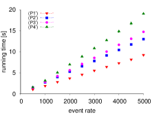
(a) in-order

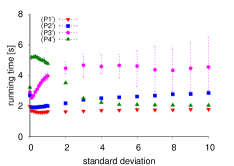
(b) out-of-order

Figure 5: Running times in a propositional setting (where each data point shows the mean of five logs together with the minimum and maximum).

Figure 5(a) shows the running times on logs with different event rates for the formulas (P1^′) to (P4^′). Figure 5(b) shows the impact when messages are received out of order for logs with an event rate 1000. We remark that some care must be taken when comparing these figures with the Figures 3(a) and (b). First, the formulas express different policies. For instance, in (P2^′) a report might discharge multiple transactions. Second, the logs for the propositional settings differ from the logs for the formulas (P1) to (P4). In particular, the events in the log files generated for the propositional settings do not account for different customers. Furthermore, we have chosen event rates that are 10 times higher. However, the running times in the propositional setting are significantly faster. In the propositional setting, our prototype usually processes an event in a fraction of a millisecond.

References

- [1] R. Alur and T. A. Henzinger. Logics and models of real time: A survey. In Proceedings of the 1991 REX Workshop on Real Time: Theory in Practice, volume 600 of Lect. Notes Comput. Sci., pages 74–106. Springer, 1992.
- [2] H. Barringer, A. Goldberg, K. Havelund, and K. Sen. Rule-based runtime verification. In Proceedings of the 5th International Conference on Verification, Model Checking and Abstract Interpretation (VMCAI), volume 2937 of Lect. Notes Comput. Sci., pages 44–57. Springer, 2004.
- [3] D. Basin, M. Harvan, F. Klaedtke, and E. Zălinescu. MONPOLY: Monitoring usage-control policies. In Proceedings of the 2nd International Conference on Runtime Verification (RV), volume 7186 of Lect. Notes Comput. Sci., pages 360–364. Springer, 2012.
- [4] D. Basin, F. Klaedtke, S. Marinovic, and E. Zălinescu. Monitoring compliance policies over incomplete and disagreeing logs. In Proceedings of the 3rd International Conference on Runtime Verification (RV), volume 7687 of Lect. Notes Comput. Sci., pages 151–167. Springer, 2013.
- [5] D. Basin, F. Klaedtke, S. Müller, and E. Zălinescu. Monitoring metric first-order temporal properties. J. ACM, 62(2), 2015.
- [6] D. Basin, F. Klaedtke, and E. Zălinescu. Failure-aware runtime verification of distributed systems. In Proceedings of the 35th International Conference on Foundations of Software Technology and Theoretical Computer Science (FSTTCS), volume 45 of Leibniz International Proceedings in Informatics (LIPIcs), pages 590–603. Schloss Dagstuhl – Leibniz Center for Informatics, 2015.
- [7] A. Bauer and Y. Falcone. Decentralised LTL monitoring. In Proceedings of the 18th International Symposium on Formal Methods (FM), volume 7436 of Lect. Notes Comput. Sci., pages 85–100. Springer, 2012.
- [8] A. Bauer, J. Küster, and G. Vegliach. The ins and outs of first-order runtime verification. Form. Methods Syst. Des., 46(3):286–316, 2015.
- [9] A. Bauer, M. Leucker, and C. Schallhart. Comparing LTL semantics for runtime verification. J. Logic Comput., 20(3):651–674, 2010.
- [10] A. Bauer, M. Leucker, and C. Schallhart. Runtime verification for LTL and TLTL. ACM Trans. Softw. Eng. Meth., 20(4), 2011.
- [11] C. Colombo and Y. Falcone. Organising LTL monitors over distributed systems with a global clock. Form. Methods Syst. Des., 49(1):109–158, 2016.
- [12] S. Feng, M. Lohrey, and K. Quaas. Path checking for MTL and TPTL over data words. In Proceedings of the 19th International Conference on Development in Language Theory (DLT), volume 9168 of Lect. Notes Comput. Sci., pages 326–339. Springer, 2015.
- [13] D. Garg, L. Jia, and A. Datta. Policy auditing over incomplete logs: Theory, implementation and applications. In Proceedings of the 18th ACM Conference on Computer and Communications Security (CCS), pages 151–162. ACM Press, 2011.
- [14] P. Goidefroid and N. Piterman. LTL generalized model checking revisited. Int. J. Softw. Tools Technol. Trans., 13(6):571–584, 2011.
- [15] T. A. Henzinger. Half-order modal logic: how to prove real-time properties. In Proceedings of the 9th Annual ACM Symposium on Principles of Distributed Computing (PODC), pages 281–296. ACM Press, 1990.
- [16] R. Koymans. Specifying real-time properties with metric temporal logic. Real-Time Syst., 2(4):255–299, 1990.
- [17] O. Maler and D. Nickovic. Monitoring temporal properties of continuous signals. In Proceedings of the Joint International Conferences on Formal Modelling and Analysis of Timed Systems (FORMATS) and on Formal Techniques in Real-Time and Fault-Tolerant Systems (FTRTFT), volume 3253 of Lect. Notes Comput. Sci., pages 152–166. Springer, 2004.
- [18] P. O. Meredith, D. Jin, D. Griffith, F. Chen, and G. Ro\cbsu. An overview of the MOP runtime verification framework. Int. J. Softw. Tools Technol. Trans., 14(3):249–289, 2012.
- [19] M. Mostafa and B. Bonakdarbour. Decentralized runtime verification of LTL specifications in distributed systems. In Proceedings of the 29th IEEE International Parallel and Distributed Processing Symposium (IPDPS). IEEE Computer Society, 2015.
- [20] J. Ouaknine and J. Worrell. On metric temporal logic and faulty turing machines. In Proceedings of the 9th International Conference on Foundations of Software Science and Computation Structures (FOSSACS), volume 3921 of Lect. Notes Comput. Sci., pages 217–230. Springer, 2006.
- [21] K. Sen, A. Vardhan, G. Agha, and G. Ro\cbsu. Efficient decentralized monitoring of safety in distributed systems. In Proceedings of the 26th International Conference on Software Engineering (ICSE), pages 418–427. IEEE Computer Society, 2004.