The First Ionization Potential Effect from the Ponderomotive Force: On the Polarization and Coronal Origin of the Alfvén Waves

Abstract

We investigate in more detail the origin of chromospheric Alfvén waves that give rise to the separation of ions and neutrals, the First Ionization Potential Effect (FIP), through the action of the ponderomotive force. In open field regions, we model the dependence of fractionation on the plasma upflow velocity through the chromosphere for both shear (or planar) and torsional Alfvén waves of photospheric origin. These differ mainly through their parametric coupling to slow mode waves. Shear Alfvén waves appear to reproduce observed fractionations for a wider range of model parameters, and present less of a “fine-tuning” problem than do torsional waves. In closed field regions, we study the fractionations produced by Alfvén waves with photospheric and coronal origins. Waves with a coronal origin, at or close to resonance with the coronal loop, offer a significantly better match to observed abundances than do photospheric waves, with shear and torsional waves in such a case giving essentially indistinguishable fractionations. Such coronal waves are likely the result of a nanoflare coronal heating mechanism, that as well as heating coronal plasmas releases Alfvén waves that can travel down to loop footpoints and cause FIP fractionation through the ponderomotive force as they reflect from the chromosphere back into the corona.

1. Introduction

The First Ionization Potential (FIP) Effect is the by now well known abundance anomaly in the solar corona and slow speed solar wind, whereby elements such as Fe, Si, and Mg with FIP less than about 10 eV, i.e. those elements that are predominantly ionized in the solar chromosphere, are enhanced in abundance in the solar corona with respect to solar photospheric values by a factor of about three. High FIP elements are generally unchanged, although He and Ne can also show abundance depletions. First discovered by Pottasch (1963), a compelling explanation in terms of the ponderomotive force arising as Alfvén waves propagate through or reflect from the chromosphere has been advanced (Laming, 2004, 2009, 2012, 2015).

The ponderomotive force, discussed in more detail in section 2 and in the Appendix, arises from the combined effects of the reflection and refraction of Alfvén waves on the plasma ions. Plasma neutrals are not affected, since the waves are fundamentally oscillations of the magnetic field. The time averaged ponderomotive force is generally directed upwards in the solar chromosphere, giving rise to an enhancement of ions over neutrals. In special conditions, a downwards pointing force can arise instead, depleting the ions to give rise to an “Inverse FIP Effect”, as seen recently near a sunspot (Doschek et al., 2015), and in the coronae of stars of later spectral type than the Sun (Wood et al., 2012).

The time varying part of the same ponderomotive force is also responsible for the excitation of acoustic waves by a parametric instability (e.g. Hollweg, 1971), and these acoustic waves can inhibit the FIP fractionation. Consequently while the explanation of the FIP Effect in terms of the ponderomotive force may be considered “compelling”, much scope remains for subtle details of the fractionation to be influenced by details of wave-wave interactions in the chromosphere, and by the precise origin of the Alfvén waves. Such topics will be a great interest for the forthcoming solar missions Solar Orbiter (Müller et al., 2013) and the Parker Solar Probe (Fox et al., 2016).

The traditional view is that Alfvén waves, presumably resulting ultimately from the mode conversion of p-modes (see e.g. Cally, 2017), or from other interactions of photospheric acoustic energy with magnetic flux tubes (see discussion in Cranmer & van Ballegooijen, 2005) are injected into a coronal loop through the chromospheric footpoints from below. Unless a coincidental match between the wave frequency and the loop resonance exists, significant reflection of waves back down to the photosphere occurs (Hollweg, 1984; van Ballegooijen et al., 2011). Alternatively, waves generated in the corona will naturally be on resonance (e.g. Ruderman & Roberts, 2002; Dahlburg et al., 2016), at least until chromospheric evaporation or other activity changes the coronal Alfvén speed or loop length. Such waves reflect from the top of the chromosphere back into the corona. One of the conclusions of this paper will be that the observed FIP Effect strongly favors these resonant waves, and hence a coronal origin for the Alfvén waves.

Further, differences may also occur between shear (or planar) and torsional Alfvén waves. Historically shear Alfvén waves, appropriate to an unstructured solar atmosphere, have received most attention, though recent observations have indicated the presence of torsional waves in spicules (De Pontieu et al., 2012; Sekse et al., 2013) and in other regions of the chromosphere and transition region (Jess et al., 2009; De Pontieu et al., 2014). Cally (2017; see also Mathioudakis et al. 2013; Jess et al. 2013) give a thorough review of solar observations and interpretations in terms of the various manifestations of planar or torsional Alfvén(ic) waves. While these different waves obey the same Alfvén wave transport equations (see e.g. Heinemann & Olbert, 1980; Khabibrakhmanov & Summers, 1997; Cranmer & van Ballegooijen, 2005), they have different parametric couplings to acoustic waves, and potentially different FIP fractionation may result.

In this paper we investigate the effect of differing origins and polarizations of Alfvén waves on the FIP fractionation pattern. Section 2 treats the coupling of torsional and shear Alfvén waves to slow mode waves, including the effects of an upward plasma flow. The fractionation is also subtly changed by this upward flow. Section 3 gives fractionation results for the open magnetic field of a coronal hole, while section 4 gives the corresponding results for a closed coronal loop. Section 5 concludes, with some technical details concerning derivations of the expression for the ponderomotive force and equations governing the torsional Alfvén waves given in Appendices.

2. Coupling to Slow Mode Waves

2.1. Torsional Alfvén Waves

Torsional Alfvén waves are rotational oscillations of a cylindrical plasma structure, of higher density than its surroundings. To keep the gas pressure perturbation zero as in an Alfvén wave, an incompressible displacement must be directed perpendicularly to the pressure gradient. Thus in a cylindrical plasma column with untwisted magnetic field, the incompressible waves are torsional oscillations (Vasheghani Farahani et al., 2010). Vasheghani Farahani et al. (2010, 2011) treat an ideal case with a discontinuity in gas pressure and density at the periphery of the (assumed circular) flux tube, whereas the possibly more familiar planar Alfvén wave applies in the case of infinite and uniform plasma. Obviously a continuum of cases will exist between these two idealizations, depending on the density or pressure gradients in the background plasma. However in what follows, we will restrict ourselves to comparing between these two limits.

The coupling of torsional Alfvén waves to slow mode waves is treated by Vasheghani Farahani et al. (2011), for the axisymmetric ($m=0$) case, extending as far as linear terms in compressible variables. We follow their treatment and extend to arbitrary $m$, where the azimuthal variation of the perturbation is given by $\exp im\phi$, and include a background density gradient as seen in the simulations of Del Zanna et al. (2005) and included in the treatment of shear Alfvén waves in Laming (2012), given by the usual hydrostatic stratification of the chromosphere. The corona is expected and observed to exhibit a filamentary structure (e.g. Dahlburg et al., 2012; Testa et al., 2013), where the transverse filament dimension is comparable to the longitudinal density scale height in the chromosphere, both of which are much smaller than the Alfvén wave wavelength. Consequently the thin flux tube approximation is valid. The linearized equation of motion is

$$\rho{\partial\delta{\bf v}\over\partial t}+\rho\left(\delta{\bf v}\cdot\nabla\delta{\bf v}\right)={\bf J}\times{\bf B}-\nabla\delta P-{\bf g}\delta\rho$$ (1)

for perturbed velocity, pressure and density $\delta{\bf v}$, $\delta P$, and $\delta\rho$ respectively, with other symbols having their usual meanings. In the $z$-direction (in cylindrical coordinates, and neglecting the displacement current, with B and g along z)

$$\rho{\partial\delta v_{z}\over\partial t}=-{1\over 4\pi}\left(\delta B_{r}{\partial\delta B_{r}\over\partial z}+\delta B_{\phi}{\partial\delta B_{\phi}\over\partial z}\right)-{\partial\delta P\over\partial z}-g\delta\rho$$ (2)

We recognize the first term in brackets $\left(\cdots\right)$ on the right hand side as the ponderomotive force. For standing waves, such as in coronal loops, it can be rewritten as

$$-{\partial\left(\delta B_{r}^{2}+\delta B_{\phi}^{2}\right)\over 8\pi\partial z}={\partial\left(\epsilon-1\right)\left(\delta E_{r}^{2}+\delta E_{\phi}^{2}\right)\over 8\pi\partial z}$$ (3)

$$= \Sigma_{j}{m_{j}c^{2}\over 2}{\partial\left(\delta E_{r}^{2}+\delta E_{\phi}^{2}\right)/B^{2}\over\partial z},$$

where $\epsilon-1=\Sigma_{k}\omega_{pk}^{2}/\Omega_{k}^{2}=c^{2}/V_{A}^{2}=\Sigma_{j}4\pi m_{j}c^{2}/B^{2}$ with $\Sigma_{k}$ being a sum over over particle species $k$ with plasma frequency $\omega_{pk}$ and cyclotron frequency $\Omega_{k}$, and $\Sigma_{j}$ being a sum over over particles $j$ each with mass $m_{j}$ in the volume in which the density is measured. This leads to an instantaneous ponderomotive force on each particle of $m_{j}c^{2}{\partial\left(\delta E_{r}^{2}/B^{2}+\delta E_{\phi}^{2}/B^{2}\right)/\partial z}/2$. In fact as shown in the Appendix A, this last form for the ponderomotive force is more general than the negative gradient of the magnetic energy, which only holds in the WKB approximation, and can be derived from the more general form within this approximation. Note the change of sign between the initial and final expressions in equation 3, due to the relative phases of $\delta B$ and $\delta E$ in the standing wave. This sign change was omitted in equation 14 of Laming (2012). To lowest order this sign change makes no difference, but when higher order terms are included, it reduces slightly the resulting slow mode wave amplitudes given in that paper.

In the $r$-direction Vasheghani Farahani et al. (2011) give (their equation 4)

$$\left[P+{B\delta B_{z}\over 4\pi}\right]_{r=0} - {A\over 2\pi}\rho{\partial\over\partial t}\left(\delta v_{r}\over r\right)-{AB\over 16\pi^{2}}{\partial^{2}\delta B_{z}\over\partial z^{2}}$$ (4)

$$= P_{ext}+{AJ^{2}\over 8\pi^{2}}-{A\Omega^{2}\over 2\pi^{2}},$$

where $J=\delta B_{\phi}/r$, $\Omega=\delta v_{\phi}/r$ and $A$ is the area of the flux tube cross section. While $J$ and $\Omega$ should be generalized for $m>0$ for our purposes, in fact ultimately these terms tend to zero in the thin flux tube approximation, leaving

$${\partial\delta P\over\partial t}=-{B\over 4\pi}{\partial\delta B_{z}\over\partial t}={B^{2}\over 4\pi}\left({\delta v_{r}\over r}+{m\delta v_{\phi}\over r}\right)\cos m\phi,$$ (5)

where we have substituted for $\partial\delta B_{z}/\partial t$ from the induction equation;

$${\partial\delta{\bf B}\over\partial t}=\nabla\times\left(\delta{\bf v}\times{\bf B}\right),$$ (6)

expanded following equation B1 in Appendix B below. Substituting for $\left(\delta v_{r}+m\delta v_{\phi}\right)/r$ from the continuity equation;

$${\partial\delta\rho\over\partial t}+\rho\nabla\cdot{\bf v}={\partial\delta\rho\over\partial t}+\rho{\partial\delta v_{z}\over\partial z}+\rho\left({\delta v_{r}\over r}+{m\delta v_{\phi}\over r}\right)\cos m\phi=0,$$ (7)

into equation 5 yields

$${\partial\delta P\over\partial t}={-B_{z}^{2}\over 4\pi\rho}\left(i\omega\delta\rho+\rho{\partial\delta v_{z}\over\partial z}\right)$$ (8)

with $\delta\rho\propto\exp\left(i\omega_{s}t\right)$. Differentiating equation 8 again with respect to $t$, and substituting from equation 2, where $c_{s}$ is the sound speed, $\delta P=\delta\rho c_{s}^{2}$, and $V_{A}=B_{z}/\sqrt{4\pi\rho}$ is the Alfvén speed, gives

$${c_{s}^{2}\over V_{A}^{2}}{\partial^{2}\delta\rho\over\partial t^{2}} = \omega_{s}^{2}\delta\rho+{\partial^{2}\delta P\over\partial z^{2}}+g{\partial\delta\rho\over\partial z}$$

$$- {\partial\over\partial z}\left\{{\rho c^{2}\over 2}{\partial\over\partial z}\left(\delta E_{r}^{2}+\delta E_{\phi}^{2}\over B_{z}^{2}\right)\right\}+{\partial\rho\over\partial z}{\partial\delta v_{z}\over\partial t}.$$

which with $\partial\rho/\partial z=\rho/L$, $i\omega_{s}\delta\rho=-\left(ik_{s}+1/L\right)\rho\delta v_{z}$, $\partial\delta\rho/\partial z=\left(ik_{s}+1/L\right)\delta\rho$ and $\partial\delta v_{z}/\partial z=ik_{s}\delta v_{z}$ (Laming, 2012) becomes

$$\delta\rho \left\{\omega_{s}^{2}\left(c_{s}^{2}+V_{A}^{2}\right)+c_{s}^{2}V_{A}^{2}\left(ik_{s}+1/L\right)^{2}+V_{A}^{2}g\left(ik_{s}+1/L\right)\right\}$$

$$= V_{A}^{2}{\partial\over\partial z}\left\{{\rho c^{2}\over 2}{\partial\over\partial z}\left(\delta E_{r}^{2}+\delta E_{\phi}^{2}\over B_{z}^{2}\right)\right\}-{i\omega\rho V_{A}^{2}\over L}\delta v_{z}.$$ (10)

The first term in curly brackets on the left hand side, $\omega_{s}^{2}c_{s}^{2}$, is new and does not appear in the treatment of shear Alfvén waves (see below, subsection 2.4), and leads to different properties of the coupling of torsional Alfvén waves to slow modes (e.g. Vasheghani Farahani et al., 2011). Identifying

$$\omega_{s} = 2\omega_{A}/n$$

$$\Re k_{s} = \sqrt{\left(2\Re k_{A}/n\right)^{2}-g^{2}/4c_{s}^{4}}$$

$$\Im k_{s} = -g/2c_{s}^{2}$$

$$L = -c_{s}^{2}/g$$ (11)

where $n$ is an integer, (see e.g. Landau & Lifshitz, 1976), we find

$$\omega_{s}^{2}\delta\rho={\partial\over\partial z}\left\{{\rho c^{2}\over 2}{\partial\over\partial z}\left(\delta E_{r}^{2}+\delta E_{\phi}^{2}\over B_{z}^{2}\right)\right\}-{i\omega\rho\over L}\delta v_{z},$$ (12)

where the new term $\omega_{s}^{2}c_{s}^{2}=4\omega_{A}^{2}c_{s}^{2}/n^{2}$ cancels exactly with the term in $4k_{A}^{2}V_{A}^{2}c_{s}^{2}/n^{2}$. Thus unlike the case of shear Alfvén waves, resonant generation of sound waves when $V_{A}=c_{s}$ does not occur with torsional Alfvén waves, as in Vasheghani Farahani et al. (2011). Integrating by parts, equation 12 can be rewritten as

$$\delta v_{z} = -{ic^{2}\over 2\omega_{s}}\left(1+ik_{s}L\over 2+ik_{s}L\right){\partial\over\partial z}\left(\delta E_{r}^{2}+\delta E_{\phi}^{2}\over B_{z}^{2}\right)$$ (13)

$$= -{i\over 2\omega_{s}}\left(1+ik_{s}L\over 2+ik_{s}L\right){\partial\over\partial z}\left(\delta v_{r}^{2}+\delta v_{\phi}^{2}\right)$$

since $\delta{\bf E}=\delta{\bf v}\times{\bf B}/c$. The parametric generation of sound waves by torsional Alfvén waves is lower than for shear Alfvén waves because the possibility of a resonance does not exist.

2.2. Inclusion of Plasma Flow

We introduce a steady plasma flow velocity ${\bf U}=U{\bf\hat{z}}$, where ${\bf\hat{z}}$ is a unit vector in the z-direction and $\partial U/\partial t=0$ into equations 1 and 7. We assume $U<<c_{s}$ for the time being, so that the background chromospheric density profile is not changed. Equation 12 becomes

$$\left(\omega_{s}^{2}+{i\omega_{s}U\over L}\right)\delta\rho={\partial\over\partial z}{\rho c^{2}\over 2}{\partial\over\partial z}\left(\delta E_{r}^{2}+\delta E_{\phi}^{2}\over B_{z}^{2}\right)$$

$$- {\partial\over\partial z}\left\{\rho U\delta v_{z}\left(ik_{s}-{1\over L}\right)-{\delta\rho U^{2}\over L}\right\}-{i\omega_{s}\rho\over L}\delta v_{z},$$

which after substituting $i\omega_{s}\delta\rho=-\left(ik_{s}+1/L\right)\rho\delta v_{z}$ and integrating by parts gives

$$\left\{\left(\omega_{s}+{iU\over L}\right)^{2}+{\omega_{s}\over k_{s}}{U\over L^{2}}\left(1+k_{s}^{2}L^{2}\right)-{ik_{s}U^{2}\over L}+{\omega_{s}^{2}\over 1+ik_{s}L}\right\}\delta v_{z}$$

$$=-i{\omega_{s}c^{2}\over 2}{\partial\over\partial z}\left(\delta E_{r}^{2}+\delta E_{\phi}^{2}\over B_{z}^{2}\right).$$ (15)

In steep density gradients, $k_{s}L<<1$ and the second term in brackets $\left[...\right]$ on the left hand side can dominate if $U>0$, reducing $\delta v_{z}$.

2.3. Back Reaction of Slow Modes on Alfvén Waves

The term on the right hand side of equation 15 is unpacked as follows

$$-i{\omega_{s}c^{2}\over 2}{\partial\over\partial z}\left(\delta E^{2}\over B_{z}^{2}\right) = -i{\omega_{s}\over 2}{\partial\over\partial z}\left(\delta B^{2}\over 4\pi\left(\rho+\delta\rho\right)\right)$$

$$\simeq -i{\omega_{s}\over 2}{\partial\over\partial z}\left({\delta B^{2}\over 4\pi\rho}\left[1-{\delta\rho\over\rho}+...\right]\right)$$

$$\simeq\omega_{s}k_{A}\delta V_{A}^{2} + \delta v_{z}\delta V_{A}^{2}\left(k_{A}k_{s}-{k_{s}^{2}\over 2}-i{k_{A}\over L}+i{k_{s}\over 2L}\right),$$

where $\delta V_{A}^{2}=\delta B^{2}/4\pi\rho$ and $\partial\delta V_{A}^{2}/\partial z=2ik_{A}\delta V_{A}^{2}$, and $i\omega_{s}\delta\rho=-\left(ik_{s}+1/L\right)\rho\delta v_{z}$ as before. The extra terms in $\delta v_{z}$ have the effect of reducing the slow mode wave amplitude in the regions of steep density gradient, where the Alfvén wave becomes evanescent (see e.g. Rakowski & Laming, 2012). Ignoring for the time being the flow velocity,

$$\delta v_{z} = {\omega_{s}k_{A}\delta V_{A}^{2}\over\omega_{s}^{2}-\delta V_{A}^{2}\left(k_{A}k_{s}-{k_{s}^{2}/2}-i{k_{A}/L}+i{k_{s}/2L}\right)}$$

$$\rightarrow {k_{A}\delta V_{A}^{2}\over\omega_{s}}\quad{\rm where}~{}\Re k_{A}\rightarrow 0,~{}\Re k_{s}\rightarrow 0$$

$$\rightarrow {\omega_{s}k_{A}\delta V_{A}^{2}\over\omega_{s}^{2}-\left(1-i/2\Re k_{A}L+1/4\Re k_{A}L\right)\delta V_{A}^{2}g^{2}/16c_{s}^{4}}$$

otherwise, after putting $\Im k_{A}=1/4L$, $\Im k_{s}=1/2L$, and $\left(\Re k_{s}\right)^{2}=4\left(\Re k_{A}\right)^{2}-g^{2}/4c_{s}^{2}$. Equations 17 indeed give lower $\delta v_{z}$ when $\Re k_{A}=0$.

2.4. Shear Alfvén Waves Revisited

We give here the corresponding equation for shear Alfvén waves,

$$\biggl{\{}\left(\omega_{s}+{iU\over L}\right)^{2}+\omega_{s}k_{s}U-{i\omega_{s}U\over L}-{ik_{s}U^{2}\over L}$$

$$-k_{s}^{2}c_{s}^{2}-ik_{s}g-\delta V_{A}^{2}\left(k_{A}k_{s}-{k_{s}^{2}\over 2}-i{k_{A}\over L}+i{k_{s}\over 2L}\right)\biggr{\}}\delta v_{z}$$

$$=-i{\omega_{s}c^{2}\over 2}{\partial\over\partial z}\left(\delta E_{r}^{2}+\delta E_{\phi}^{2}\over B_{z}^{2}\right).$$ (18)

This is slightly different to equation 14 from Laming (2012) to the same order in $\delta v_{z}$ for an assumed isothermal chromosphere ($\gamma=1)$, (and with the sign of the ponderomotive force corrected), although numerical results are very similar. The reason for the difference is that we have taken a linear relation between $\delta\rho$ and $\delta v_{z}$, $i\omega_{s}\delta\rho=-\left(ik_{s}+1/L\right)\rho\delta v_{z}$, whereas Laming (2012) took higher orders into account.

2.5. Slow Mode Waves from Convection

The different couplings of shear and torsional Alfvén waves to slow mode waves are the features that give rise to the subtly different fractionation patterns the waves produce, as will be shown below. Another source of slow mode wave derives from convection below the photosphere. Heggland et al. (2011) model this process, resulting in upgoing acoustic waves in the chromosphere, with an amplitude approximately constant with altitude of order 7.0 km s^-1 (see also Figure 3ab in Vieytes et al., 2005; Carlsson et al., 2015; Kato et al., 2011) in the region where strong wave transmission upwards from the photosphere occurs. The amplitude growth that would be expected as the wave travels upwards in progressively decreasing density of the chromosphere is presumably balanced by energy losses to radiation and thermal conduction. This wave amplitude is added in quadrature to the amplitude of parametrically generated slow mode waves for use in model calculations. If the resulting amplitude is greater than the local sound speed, such that a shock would develop, all fractionation is switched off. The rationale for this is that the discontinuity associated with a shock front will cause cause reflection of upgoing sound waves once overtaken by the shock. Downgoing and upgoing waves can interact and cause a cascade to microscopic scales. The mixing connected with this cascade will inhibit all further fractionation.

2.6. Model Calculations

We model Alfvén wave propagation on a model loop anchored in the chromosphere at each end, largely following the extensive description given in Laming (2015). The chromospheric model is taken from Avrett & Loeser (2008), which gives the plasma density, electron temperature, and ionization fraction of hydrogen as a function of altitude above the photosphere. Ionization fractions for other elements are calculated using atomic collisional data tabulated in Mazzotta et al. (1998), Bryans et al. (2009), Nikolić et al. (2013) and Kingdon & Ferland (1996). Photoionization rates are evaluated using coronal spectra incident from above based on Vernazza & Reeves (1978) or more modern calculations Huba et al. (e.g. 2005), with photoionization cross sections from Verner et al. (1996).

Alfvén wave propagation is treated in a chromospheric magnetic field model given by Athay (1981), typically with an expansion of a factor of 5 between the photosphere and corona, where the field is straight and uniform (the coronal loop is taken to be straightened out with a chromosphere at each end). The Alfvén wave transport equations are given by Cranmer & van Ballegooijen (2005) and Laming (2015), and are

$${\partial I_{\pm}\over\partial t}+\left(u\mp V_{A}\right){\partial I_{\pm}\over\partial z}=\left(u\pm V_{A}\right)\left({I_{\pm}\over 4L}+{I_{\mp}\over 2L_{A}}\right)$$ (19)

where ${\bf I}_{\pm}=\delta{\bf v}\pm\delta{\bf B}/\sqrt{4\pi\rho}$ are the Elsässer variables representing waves propagating in the $\mp$ z-directions.

Given the Alfvén wave profile, the ponderomotive force is calculated from equations A2 or A7, divided by a further factor of two to account for the average force in terms of the peak electric field fluctuation $\delta E$. The chromospheric model employed here is not specifically a loop footpoint chromosphere, and so any effect of the coronal Alfvén waves on the chromospheric structure must be accounted for. This is treated by Laming (2015), who rewrites the equation for a gravitationally stratified hydrostatic equilibrium, including the ponderomotive force, which in turn depends on the resulting density gradient. This modification begins to set in at ponderomotive accelerations around $10^{6}$ cm s^-2 and ultimately leads to saturation. It makes a small difference to the fractionations calculated here, but is included because it also allows fractionations relative to hydrogen to be computed (instead of just oxygen as was done until now, e.g. Laming, 2015). This modified expression for the ponderomotive acceleration is

$$a={a_{0}\over 1+\left(\xi_{h}/4\right)\left(\nu_{eff}/\nu_{hi}\right)\left(\delta v^{2}/v_{h}^{2}\right)}$$ (20)

where $\nu_{eff}=\nu_{hi}\nu_{hn}/\left(\xi_{h}\nu_{hn}+\left(1-\xi_{h}\right)\nu_{hi}\right)$ is the effective collision frequency of element $h$ (in this case hydrogen) in terms of its collision frequencies when ionized $\nu_{hi}$, and when neutral $\nu_{hn}$, and $v_{h}^{2}=k_{\rm B}T/m_{h}+v_{sm}^{2}+v_{\mu turb}^{2}$ is the square of the hydrogen speed, in terms of its thermal speed, the amplitude of slow mode waves propagating through the chromosphere, and the amplitude of microturbulence in the chromospheric model. Since the ponderomotive force separates ions from neutrals, its effect on the background plasma to smooth out density gradients depends on the coupling between ionized and neutral hydrogen, and is strongest in regions where hydrogen is fully ionized ($\xi=1$). This modification to the density scale length is also applied to $L$ in equation 11.

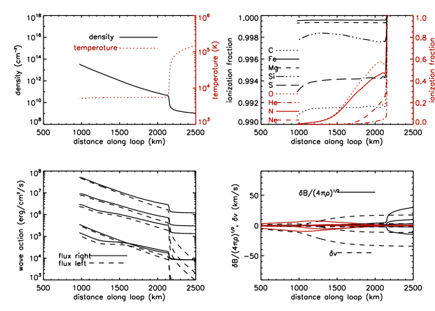
Figure 1.— The chromospheric portion of the open field model. Top left shows the density and temperature structure of the chromosphere. Top right shows chromospheric ionization fractions for selected elements, low FIPs in black to be read on the left hand axis, and high FIPs in red to be read on the right. Bottom right show the variation of the components of the Elsässer variables for the five wave frequencies considered, real parts in black and imaginary parts in red, and bottom left shows the corresponding wave energy fluxes.

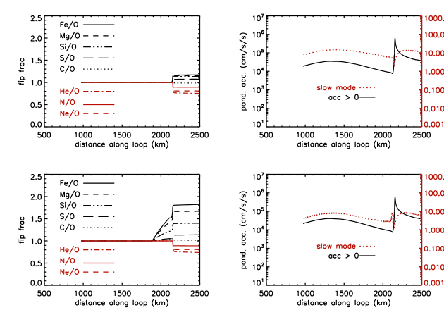
Figure 2.— FIP fractionation for selected elements (left) and ponderomotive acceleration and associated slow mode wave amplitude, in red, and to be read on the right hand axis (right). The top panels show results for shear Alfvén waves, the lower ones for $m=0$ torsional Alfvén waves. The flow velocity is taken to be 0.1 km s^-1 at a chromospheric density of $10^{10}$ cm^-3, and is insignificantly different from the case with zero flow velocity.

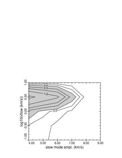
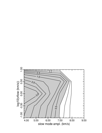
Figure 3.— Sensitivity of the Fe/O fractionation presented as logarithmic contours in the upflow velocity - slow mode amplitude plane. Left hand panel shows shear Alfvén waves, right hand panel shows torsional Alfvén waves. Fractionations greater than 2 that violate observational values are shaded gray.

With these definitions, the fractionation by the ponderomotive acceleration for element $k$ (with ions and neutrals of element $k$ denoted by $ki$ and $kn$ respectively) is given by solving the momentum equations

$$\rho_{ki}u_{ki}{\partial u_{ki}\over\partial z}+{\partial P_{ki}\over\partial z} = -\rho_{ki}g-\rho_{ki}\nu_{ki}\left(u_{ki}-u\right)+\rho_{ki}a$$

$$\rho_{kn}u_{kn}{\partial u_{kn}\over\partial z}+{\partial P_{kn}\over\partial z} = -\rho_{kn}g-\rho_{kn}\nu_{kn}\left(u_{kn}-u\right).$$ (21)

These are the same momentum equations as given elsewhere (e.g. Laming, 2015), but with inertial terms added on the left hand side to account for the plasma flow. Following Schwadron et al. (1999) we form $\nu_{kn}\partial P_{ki}/\partial z+\nu_{ki}\partial P_{kn}/\partial z$ to find

$${\partial\over\partial z}\left(P_{k}+\rho_{k}u_{k}^{2}\right)={\nu_{eff}\xi_{k}a\rho_{k}\over\nu_{ki}}$$ (22)

where $P_{ki}=\xi P_{k}$, $P_{kn}=\left(1-\xi\right)P_{k}$, $\rho_{ki}=\xi\rho_{k}$, $\rho_{kn}=\left(1-\xi\right)\rho_{k}$, and we have approximated

$$\rho_{k}\nu_{eff}\left({\xi_{k}\over\nu_{ki}}u_{ki}{\partial u_{ki}\over\partial z}+{1-\xi_{k}\over\nu_{kn}}u_{kn}{\partial u_{kn}\over\partial z}\right) \simeq \rho_{k}u_{k}{\partial u_{k}\over\partial z}$$ (23)

$$= {\partial\rho u_{k}^{2}\over\partial z}$$

since $\rho_{k}u_{k}=$ constant in the final step. We put $P_{k}=\rho_{k}\left(kT/m_{k}+\Sigma v_{||}^{2}/2\right)$ where the terms in brackets are the ion thermal speed and a quadrature sum over all nonthermal longitudinal velocity oscillations, slow mode waves, microturbulence, etc. The fractionation is evaluated from equation 22 by splitting the integration up into pieces where $kT/m_{k}+\Sigma v_{||}^{2}/2+u_{k}^{2}$ is approximately constant and calculating

$${\rho_{k}\left(z_{u}\right)\over\rho_{k}\left(z_{l}\right)}=\exp\left\{\int_{z_{l}}^{z_{u}}{2\xi_{k}a\nu_{eff}\over\nu_{ki}\left(2kT/m_{k}+\Sigma v_{||}^{2}+2u_{k}^{2}\right)}dz\right\}.$$ (24)

in each piece, where $u_{k}$ is specified to give zero fractionation in the absence of $a$, and where the constant of integration also as been chosen to keep $\rho_{k}\left(z_{u}\right)=\rho_{k}\left(z_{l}\right)$ when $a=0$. The total fractionation is then the product of all the individual pieces.

3. Open Magnetic Field

We first demonstrate the effects of shear and torsional Alfvén waves in open magnetic field. The basic chromospheric model and Alfvén wave propagation are illustrated in Fig. 1, and follow very closely the set up in Laming (2012, 2015). The magnetic field is taken from Banaszkiewicz et al. (1998) and matched to the chromospheric magnetic field taken from Athay (1981). The density profile is specified to match that in equation 3 of Cranmer & van Ballegooijen (2005). One departure from previous work is that we now include an outward flow velocity. This does not affect the Alfvén wave propagation much, since everywhere the flow is significantly sub-Alfvénic, but as will be seen below does have an effect on the generation of slow mode waves in the regions of strong density gradient.

Equations 19 are integrated starting from 500,000 km altitude back to the chromosphere. At the coronal start point, the outgoing Alfvén waves dominate (Cranmer & van Ballegooijen, 2005). Five waves are simulated, with frequencies and amplitudes chosen to match Fig. 3 in Cranmer et al. (2007) and for example Figs. 9 or 15 in Cranmer & van Ballegooijen (2005). The four panels of Fig. 1 show the chromospheric portion of the solution, with the density and temperature structure of the model chromosphere (top left), and ionization balance profiles for various important elements (top right; low FIP elements in black to be read on the left hand $y$-axis, high FIP elements in red to be read on the right hand $y$-axis), the left and right going wave energy fluxes (bottom left) and the profiles of the components of the Elsässer variables (bottom right).

Figure 2 shows the elemental fractionations (left panels) and the profiles of ponderomotive acceleration and slow mode wave amplitude (right panels). The top half shows the results for a shear Alfvén wave, the bottom for the torsional Alfvén wave. The difference in fractionation arises from the different coupling to the slow mode waves. We have assumed an upward flow speed of 0.1 km s^-1 where the chromospheric density is $10^{10}$ cm^-3 (see below for discussion and justification), which gives essentially the same results for velocity put equal to zero. At an altitude of 1200 km, the slow mode wave energy density is about 1 erg cm^-3, which if the wave is moving in one direction only corresponds to a flux of about $5\times 10^{5}$ ergs cm^-2s^-1. Cranmer & Woolsey (2015) consider acoustic waves fluxes of this magnitude (and larger) as a result of ponderomotive driving by chromospheric Alfvén waves, although they do not compute the coupling explicitly. Arber et al. (2016) and Brady & Arber (2016) do compute this coupling, and also find ponderomotive accelerations and slow mode wave amplitudes broadly consistent with Fig. 2. These authors however do not see the reduction in slow mode wave amplitude in the region of steep density gradient according to equation 17 above, presumably because they model propagating slow mode waves generated deeper in the chromosphere.

Table 1Open Field Fractionations.

Ratio	shear			torsional			ACE			Ulysses		UVCS
	0	0.1	1.0 km s-1	0	0.1	1.0 km s-1	Solar Max.	Genesis	Solar Min	PCH	CH
He/O	0.75	0.75	0.74	0.74	0.74	0.71	0.51	0.48	0.45			0.45-0.55
C/O	0.97	0.99	0.98	1.00	1.02	1.04	1.11	1.15	1.16	1.22	1.23	0.9-1.1
N/O	0.88	0.89	0.88	0.88	0.89	0.87				1.11	1.11
Ne/O	0.80	0.81	0.79	0.80	0.81	0.79	0.57	0.60	0.67	0.63	0.63	0.3-0.4
Mg/O	1.13	1.15	1.18	1.57	1.67	2.40	1.89	1.61	1.37	1.55	1.54	0.95-2.45
Si/O	1.11	1.14	1.16	1.34	1.40	1.79	2.60	2.40	1.99	1.74	1.80	0.9-1.8
S/O	1.06	1.07	1.08	1.11	1.14	1.22				2.19	2.35
Fe/O	1.14	1.17	1.21	1.70	1.82	2.79	2.08	1.90	1.56	1.41	1.43	0.65-1.35

With the upflow speed increased to 1.0 km s^-1 at a chromospheric density of $10^{10}$ cm^-3, the slow mode wave amplitudes in the region of strong fractionation are decreased by the addition of the terms in $U$ and $U^{2}$ in equations 15 and 18, and the fractionation is increased. Interestingly there is now a stronger difference between shear and torsional Alfvén waves, with the latter producing stronger fractionation. These results are summarized in Table 1, and compared to various observations. The “ACE” observations come from analysis of reprocessed data from the Advanced Composition Explorer (ACE) by Pilleri et al. (2015), where we quote the coronal hole measurements for solar maximum (1999-2001), solar minimum (2006-2009), and for measurements during 2001-2004, the period of operation of the Genesis mission. The Ulysses results for polar coronal holes (PCH) and low latitude coronal holes (CH) come from a similar reprocessing of the Ulysses archive given in von Steiger & Zurbuchen (2016), while the UVCS results come from remotely sensed spectroscopic measurements with the UltraViolet Corona-Spectrograph (UVCS) on SOHO reported by Ko et al. (2006). Taking a proton flux in the fast wind at 1 AU of $\sim 2\times 10^{8}$ cm^-2s^-1 translates to a flux at the solar surface of $\sim 10^{13}$ cm^-2s^-1. At a density of $10^{10}$ cm^-3, the upward flow velocity implied is $10^{3}/f$ cm s^-1, where $f$ is the area filling factor of the flow in the coronal hole, and the speeds taken above correspond to $f=0.1$ and $f=0.01$.

The differences between shear and torsional Alfvén waves are explored further in Fig 3. Contours of the Fe/O ratio are plotted in the parameter space defined by the upward flow speed and the chromospheric slow mode wave amplitude resulting from convection. Hitherto we have assumed an amplitude of 7 km s^-1, but here we consider values between 4 and 9 km s^-1. We also consider a wider range of upflow speeds than above, tacitly assuming that the upflow is driven by the ${\bf J}\times{\bf B}$ term in the momentum equation, as would be the case for a Type II spicule, leaving the chromospheric density profile unchanged. Contours for shear Alfvén waves are plotted in Fig. 3a, and for torsional Alfvén waves in Fig. 3b. The shaded regions correspond to Fe/O $>2$, and is the region that would violate most observations of fractionation in the fast wind. We can see that for shear waves, observational constraints can be satisfied for a much wider range of upflow speeds and slow mode wave amplitudes than is the case for torsional waves, because shear wave driver generates more parametric slow modes that stabilize the fractionation than does the torsional wave driver. Since the slow mode wave amplitude in the chromosphere is inevitably variable, (e.g. Heggland et al., 2011) we argue that shear Alfvén waves are more plausible.

Such an inference is of some interest. Cranmer & van Ballegooijen (2005) describe how photospheric sound waves can initiate kink oscillations in flux tubes that travel up to the corona. Upon reaching the corona where the initially isolated photospheric flux tubes merge, the kink oscillation becomes Alfvénic, either Alfvén or fast mode (depending on magnetic geometry) and parallel propagating. In a homogenous corona, these would be shear Alfvén waves, whereas inhomogeneity in the coronal plasma, or vortical photospheric motions might result in torsional coronal Alfvén waves. Verth & Jess (2016), following Goossens et al. (2014), illustrate how a kink mode may mode convert to a $m=1$ torsional Alfvén wave. The difference between shear and torsional waves is not necessarily negligible. Vasheghani Farahani et al. (2012) argue that torsional Alfvén wave undergo a slower parallel nonlinear cascade than do shear Alfvén waves, which could have implications for coronal heating and solar wind acceleration, although the effect is largest when sound and Alfvén speeds are equal.

Requerey et al. (2015) observe the dynamics of quiet sun magnetic structures. In such cases, torsional oscillations act to stabilize multi-threaded magnetic filaments, whereas planar perturbations corresponding to the forcing by granular motions tend to shred the structure. The observed lifetimes and morphological changes of magnetic flux concentrations strongly suggest perturbation by granular convection, and not the characteristic torsional oscillations of a thin flux tube, again consistent with our inference above. On the other hand Stangalini et al. (2017) see elliptically polarized kink oscillations of chromospheric small-scale magnetic elements (SSMEs), which would reduce slow mode wave excitation (circularly polarization would suppress it completely).

Lastly, several authors (e.g. De Pontieu et al., 2011) have in recent years suggested that a significant fraction of the solar corona and wind could be the result of chromspheric spicules, more specifically “Type II Spicules”, that accelerate material straight out of the chromosphere at speeds up to 100 km s^-1 (Martínez-Sykora et al., 2013). Evidence exists for both transverse and torsional oscillations (Sekse et al., 2013), though Raouafi et al. (2016) suggest that the torsional motion might be due to the unwinding of a flux rope rather than an actual torsional wave. Observed amplitudes are comparable to those in the open field model above. Figure 3 shows the fractionations expected for shear and torsional waves, assuming the same wave spectrum as for the coronal hole considered above. FIP fractionation essentially disappears at upflow speeds comparable to the sound speed ($\sim 8$ km s^-1) and above, as seen for example in polar jets by Lee et al. (2015). We follow Klimchuk & Bradshaw (2014) and Lionello et al. (2016) and argue therefore that Type II spicules cannot be a significant source of plasma to supply the solar corona or slow speed solar wind, because no means exists within such a model to provide the FIP fractionation. All fractionated plasma must move up to the corona in a more gradual fashion.

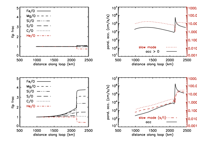
Figure 4.— Fractionations (left) and ponderomotive acceleration/slow mode wave amplitude (right) for a closed loop. The top panels show the case with similar waves (assumed shear) injected upwards from one footpoint as in the open field case. The bottom panels show the case with one wave resonant with the loop, developing higher ponderomotive acceleration and fractionation. Slow mode amplitudes are indicated for both shear (dotted) and torsional (dashed) resonant waves.

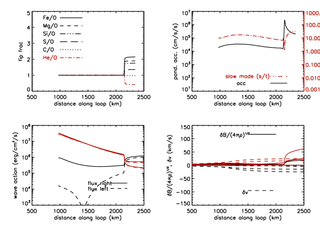
Figure 5.— Top panels show fractionations (left) and ponderomotive acceleration/slow mode wave amplitude (right) for a closed loop with both a resonant wave and three and five minute waves injected from the footpoint. Bottom panels show the wave energy fluxes (left), with the resonant wave in black and the three and five minute photospheric waves in red, and components of the Elsässer variables (right), with real parts in black, imaginary parts in red.

4. Closed Magnetic Loop

We now consider a closed magnetic loop, and demonstrate the effect of a resonance in the coronal magnetic structure. The loop is taken to be 75,000 km long, with a coronal magnetic field of 10 G. The chromospheric upflow speed at a density of $10^{10}$ cm^-3 is 0.1 km s^-1. Although we do not consider the coronal consequence of this flow, we presume it to be associated with evaporation, one of the processes by which mass is supplied to the corona. Figure 4 shows the fractionations (left) and ponderomotive acceleration/slow mode wave amplitudes (right) for this case. The top panels show a case with three minute and five minute (see e.g. Heggland et al., 2011) Alfvén waves injected at the footpoint, here assumed to be shear Alfvén waves, and with similar amplitudes to those in the open field case. The fractionation is in all respects very similar to that in the open field case with the same flow velocity of 0.1 km s^-1 (see Fig. 2, and note the different vertical scale). He/O is depleted by the same amount, $0.75$, and a similarly weak FIP fractionation is produced. The bottom panels show a case with one resonant wave (taken to be a shear or torsional Alfvén wave) with a frequency $\omega=V_{A}/L=0.0435$ rad s^-1 (the fundamental, period = 2.4 minutes), presumed to have a coronal origin. The amplitude of the coronal wave in this model is about 90 km s^-1, at a density of about $7\times 10^{8}$ cm^-3 at the loop apex. Much stronger FIP fractionation results, with a depletion of He/O by about 0.5.

Figure 5 shows in the top panel the fractionations and ponderomotive acceleration/slow mode wave amplitudes for a model where both sets of waves are present, i.e. the three and five minute Alfvén waves propagating up from the footpoint and the coronal resonant wave. Here the depletion of He/O is even stronger, at 0.4, but the FIP fraction is now intermediate between the two cases above. This arises because the extra slow mode waves produced by the upcoming Alfvén waves inhibit fractionation low in the chromosphere, while the He depletion which occurs only at the top of the chromosphere near the strong density gradient is relatively unaffected. The lower two panels of Fig. 5 show the wave energy fluxes (left) and the wave amplitudes $\delta v$ and $\delta B/\sqrt{4\pi\rho}$ (right). In each case the resonant coronal wave is shown as a black line, while the nonresonant waves from the footpoint are shown as red lines.

The results from Figs. 4 and 5 are summarized in Table 2, and compared with various observations (Zurbuchen et al., 2002; von Steiger et al., 2000; Bryans et al., 2009). The model chromosphere used here (Avrett & Loeser, 2008) connects with a fairly low density corona (few $\times 10^{8}$ cm^-3), resulting in high predicted coronal Alfvén wave amplitudes. Higher coronal densities require lower coronal Alfvén wave amplitudes to produce the necessary FIP fractionation, with wave amplitude going approximately as $1/\sqrt{\rho}$ for a standing wave.

Table 2FIP Fractionations in Closed Magnetic Field

	models 75,000km			100,000 km	observations
Ratio	bkgd	cor	bkgd+cor	bkgd	a	b	c
He/O	0.75	0.46/0.44	0.41/0.40	0.21	0.68-0.60	0.29-0.75
C/O	0.95	1.07/1.07	0.98/0.97	0.99	1.36-1.41	1.06-1.37
N/O	0.87	0.74/0.74	0.72/0.72	0.55	0.72-1.32	0.22-0.89
Ne/O	0.79	0.60/0.60	0.56/0.56	0.36	0.58	0.38-0.75
Na/O	1.10	3.68/3.77	2.07/2.08	5.48			7.8${+13\atop-5}$
Mg/O	1.08	3.11/3.31	1.90/1.91	4.38	2.58-2.61	1.08-2.36	2.8${+2.3\atop-1.3}$
Al/O	1.08	2.91/3.08	1.93/1.94	4.45			3.6${+1.7\atop-1.2}$
Si/O	1.07	2.40/2.51	1.77/1.79	3.55	2.49-3.11	1.36-3.24	4.9${+2.9\atop-1.8}$
S/O	1.02	1.51/1.54	1.37/1.38	1.88	1.62-1.92	1.23-2.68	2.2$\pm 0.2$
K/O	1.10	3.94/4.30	2.17/2.20	6.11			1.8${+0.4\atop-0.6}$
Ca/O	1.10	3.90/4.26	2.17/2.19	6.13			3.5${+4.3\atop-1.9}$
Fe/O	1.09	3.79/4.13	2.17/2.20	6.00	2.28-2.90	0.96-2.46	7.0${+1.4\atop-1.2}$

Figure 6.— Left: Fractionations of Fe/O (dashed lines) and He/O (solid line) as a function of coronal wave frequency for the model $10^{5}$ km loop. At the fundamental and first harmonic the Fe/O maximizes and the He/O minimizes, coming closest to observations at these points. Right: Same fractionations as a function of loop length for 3 and 5 minute footpoint waves. The resonance at $10^{5}$ km corresponds to 3 minute waves entering the loop.

5. Discussion and Conclusions

In order to reproduce FIP fractionation, or depletions of He/O beyond about 0.7, the presence of a resonant Alfvén wave appears necessary. Kasper et al. (2012) and more recently Kepko et al. (2016) have identified slow speed solar wind regimes where the He abundance (usually relative to H) can be as low as 1% - 2%. Rakowski & Laming (2012) found that resonant waves on longer loops with weaker magnetic fields produced the most significant He depletions. While FIP fractionation can come from coronal or photospheric waves, the He depletion requires the ponderomotive acceleration to be concentrated at the top of the chromosphere, where He is neutral but where O and H are becoming ionized. This only happens if waves are impinging on the chromosphere from the top, and being reflected back upwards again. This probable necessity of resonant waves implies a coronal origin for the waves, presumably as a result of nanoflares (e.g. Dahlburg et al., 2016).

The importance of resonant waves is emphasized further in Fig. 6. The left panel shows the fractionations of Fe/O and He/O as a function of wave frequency for the model loop introduced above. The calculations are normalized so the same total wave energy is present in the chromosphere-loop-chromosphere structure, just distributed differently as the resonant properties change. At the loop fundamental, (0.0435 rad s^-1) and the first harmonic, the Fe/O fractionation increases to about 4-8, and the He/O ratio decreases to about 0.5. In between these resonances, He/O is close to being unfractionated, while a mild FIP effect appears in Fe/O, comparable to open field values (see Table 1). Notice also that the resonances in the fractionation are not sharp. They have a finite width of order 0.01 rad s^-1, a significant fraction of the wave angular frequencies themselves, since the waves reflect from a range of chromospheric heights and not from a sharp boundary. These resonances would be even broader if we allowed for coronal wave damping, by introducing an imaginary part in the wave frequency. The important point about the width of these resonances is that while resonance is required, such that a coronal wave origin is most likely, it need not be precise. Changes in the loop resonant frequency due to changes in magnetic field by reconnection, or changes in loop plasma density due to chromospheric evaporation are unlikely to destroy the fractionation, except arguably in flares.

The right panel of Fig. 6 shows a similar calculation but this time with just the 3 and 5 minutes waves, with fractionation shown as a function of loop length. An “accidental” resonance occurs at a loop length of 100,000 km, where the three minute waves can become trapped in the loop. At this location, the Fe/O fractionation increases and the He/O ratio decreases, similarly to the resonances above. The fractionation pattern at 100,000 km is given in the fifth column of Table 2. Since a large fraction of the wave travel time from one footpoint to the other occurs inside the chromosphere at each end, the corresponding resonance for the five minutes wave occurs not at 5/3 times 100,000 km but at a loop length longer than 200,000 km. The coronal magnetic field in these examples is rather weak, at 10 G, and the loop lengths required for resonance are rather long, so it appears unlikely than an “accidental” resonance with photospheric three or five minute wave will happen frequently in a realistic coronal loop. Instead, an explanation of loop resonance in terms of waves generated within the coronal loop appears more plausible.

Candidate processes for production of Alfvén waves in the solar corona are Alfvén resonance (e.g. Ruderman & Roberts, 2002) or nanoflares (e.g. Dahlburg et al., 2016). In the former case torsional $m=1$ Alfvén waves result from the mode conversion of a kink oscillation at the plasma layer within a loop where the Alfvén wave transit time from one loop footpoint to the other matches the kink oscillation period (e.g. Jess & Verth, 2016). In the latter case the shear Alfvén waves could also be produced. The different FIP fractionations produced by shear and torsional Alfvén waves appear to be too subtle for a reliable diagnosis of the Alfvén wave polarization. More promising seems to be the observations of strong non-thermal line broadening spatially coincident with regions of strong FIP fractionation in an active region observed by Baker et al. (2013). The line broadening is presumably due to longitudinal waves, being observed just above loop footpoints on the solar disk. With this interpretation, shear Alfvén waves are favored by the wave amplitudes required. Torsional Alfvén waves do not produce strong enough slow modes to match the observations.

The preference for shear Alfvén waves generated in the corona suggests a nanoflare heating model. Based partly on the simulations in Dahlburg et al. (2016; see also Kigure et al. 2010), we argue that coronal nanoflares release Alfvén waves and heat. The Alfvén waves cause FIP fractionation at loop footpoints magnetic connected to the nanoflare site, followed by evaporation as the electrons conduct the heat down to the chromosphere. In such a scenario, the waves are likely to be in resonance with the coronal loop, reproducing the fractionation as shown in Fig. 6. The reconnection of a closed loop filled with plasma in such a manner with open field is most likely the source of the slow speed solar wind (e.g. Lynch et al., 2014; Raouafi et al., 2016). Also such a scenario will require a coronal Alfvén speed greater than the speed of electron thermal conduction. It is possible that this requirement is easier to meet in longer loops, where the thermal conduction front has to travel further to the loop footpoints and can become more degraded with distance.

Much more work remains to be done on coronal abundance anomalies and the associated wave physics responsible for them. This paper makes an attempt to show how the physics of the fractionation places constraints on the mechanism of coronal heating and mass supply in completely complementary ways to traditional methods of observation and inference. The focus on the Alfvén waves and their polarizations and resonance probes different properties of the coronal heating mechanism, and in connection with in situ observations may also be hoped to yield insight into the origin of the solar wind in the forthcoming era of the Parker Solar Probe and Solar Orbiter.

Appendix A Alternative Routes to the Ponderomotive Force

Laming (2009, 2015) give derivations by writing down the Lagrangian for a system of particles and waves, and using the known result for the partitioning of energy between kinetic, magnetic and electric in an Alfvén wave. In subsection 2.2 above, it is derived from the MHD momentum equation. Curiously, the more fundamental form of the expression does not come directly from the MHD equation, but requires further manipulation.

First, consider the force per unit volume, $f_{z}$ on the polarization and magnetization induced by turbulence in the plasma

$$f_{z}=\delta{\bf P}\cdot{\partial\delta{\bf E}\over\partial z}+\delta{\bf M}\cdot{\partial{\bf B}\over\partial z}.$$ (A1)

We put $\delta{\bf P}=\left(\epsilon-1\right)\delta{\bf E}/4\pi$ and $\delta{\bf M}=-\partial F/\partial{\bf B}$ where $F=-\epsilon\delta{\bf E}\cdot\delta{\bf E}/8\pi$ is the magnetic Helmholtz Free Energy of the plasma in the presence of the wave (see equation 14.1 in Landau et al., 1984). Substituting,

$$f_{z}={\epsilon-1\over 4\pi}\delta{\bf E}\cdot{\partial\delta{\bf E}\over\partial z}+{\partial\epsilon\over\partial{\bf B}}{\delta{\bf E}\cdot\delta{\bf E}\over 8\pi}{\partial{\bf B}\over\partial z}={\rho c^{2}\over 2B^{2}}{\partial\delta E^{2}\over\partial z}-{\rho c^{2}\delta E^{2}\over B^{3}}{\partial{\bf B}\over\partial z}={\rho c^{2}\over 2}{\partial\over\partial z}\left(\delta E^{2}\over B^{2}\right)$$ (A2)

where we have put $\epsilon=1+\omega_{pi}^{2}/\Omega_{i}^{2}=1+c^{2}/V_{A}^{2}=1+4\pi\rho c^{2}/B^{2}$, the only wave property required in this approach.

Lundin & Guglielmi (2006) give a similar treatment, but based on single particle dynamics in the external magnetic field $\left(0,0,B_{z}\right)$ and the electric field of the Alfvén wave $\left(\delta E_{x}\exp i\omega t,0,0\right)$. With

$$i\omega mv_{x} = e\delta E_{x}+ev_{y}B_{z}/c$$ (A3)

$$i\omega mv_{y} = -ev_{x}B_{z}/c,$$ (A4)

the Lorentz force on a particle of mass $m$ and charge $e$, we solve to find

$$v_{x} = -{i\omega e\delta E_{x}/m\over\omega^{2}-\Omega^{2}}$$ (A5)

$$v_{y} = {\Omega e\delta E_{x}/m\over\omega^{2}-\Omega^{2}}.$$ (A6)

The electric field in the $z$-direction which produces the ponderomotive force is $\delta E_{z}=-v_{x}\delta B_{y}/c$, where $\delta B_{y}$ is the internal magnetic field of the wave, so the total ponderomotive force on a single particle $\tilde{f}_{z}$ is given by

$$\tilde{f}_{z}=-ev_{x}\delta B_{y}/c+M{\partial B\over\partial z}$$ (A7)

where $\delta B_{y}=\left(ic/\omega\right)\partial\delta E/\partial z$ and $M=exv_{y}/c=ev_{x}v_{y}/i\omega c$ is the magnetic moment of the particle. Substituting

$$\tilde{f}_{z}=-{e^{2}\delta E_{x}/m\over\omega^{2}-\Omega^{2}}{\partial\delta E\over\partial z}-{e^{3}\over m^{2}c}{\delta E_{x}^{2}\Omega\over\left(\omega^{2}-\Omega^{2}\right)^{2}}{\partial B\over\partial z}$$ (A8)

which for $\omega<<\Omega$ reduces to

$$\tilde{f}_{z}={mc^{2}\over 2}{\partial\over\partial z}\left(\delta E_{x}^{2}\over B^{2}\right).$$ (A9)

Alternatively, and more generally, Pitaevskiĭ (1961) and Washimi & Karpman (1976) consider the change induced in $\epsilon$, and hence $F$, the total free energy, by the passage of a wave. With $F_{0}$ taken to be the the total plasma free energy in the absence of wave fields,

$$\delta\epsilon = -\left(\delta{\bf r}\cdot\nabla\right)\epsilon-{\partial\epsilon\over\partial\rho}\delta\rho\nabla\cdot\delta{\bf r}+{\partial\epsilon\over\partial{\bf B}}\left(\delta{\bf r}\cdot\nabla\right){\bf B}$$ (A10)

$$\delta F_{0} = -\left(\delta{\bf r}\cdot\nabla\right)F_{0}-{\partial F_{0}\over\partial\rho}\delta\rho\nabla\cdot\delta{\bf r}$$ (A11)

where a term in $\partial F_{0}/\partial{\bf B}=0$ in the absence of waves and plasma magnetization. Then the perturbed plasma free energy with waves present, $\delta F$, is

$$\delta F=\int\delta F_{0}-{\delta E^{2}\over 8\pi}\delta\epsilon dV=\int\left(\delta{\bf r}\cdot\nabla\right)\left[-F_{0}+{\partial F_{0}\over\partial\rho}\delta\rho-{\delta E^{2}\over 8\pi}{\partial\epsilon\over\partial\rho}\delta\rho\right]-{\delta E^{2}\over 8\pi}\left[-\left(\delta{\bf r}\cdot\nabla\right)\epsilon+{\partial\epsilon\over\partial{\bf B}}\left(\delta{\bf r}\cdot\nabla\right){\bf B}\right]dV,$$ (A12)

where terms involving $A\nabla\cdot\delta{\bf r}$ where $A$ is a scalar have been integrated by parts to give $-\delta{\bf r}\cdot\nabla A$. Equating $\delta F=-\int{\bf f}\cdot\delta{\bf r}dV$ yields

$${\bf f} = -\nabla\left[{\partial F_{0}\over\partial\rho}\delta\rho-F_{0}\right]+{1\over 8\pi}\nabla\left(\delta E^{2}\rho{\partial\epsilon\over\partial\rho}\right)-{\delta E^{2}\over 8\pi}\left[\nabla\epsilon-{\partial\epsilon\over\partial{\bf B}}\nabla{\bf B}\right]$$ (A13)

$$= -\nabla\delta P+{1\over 8\pi}\nabla\left(\left(\epsilon-1\right)\delta E^{2}\right)-{\delta E^{2}\over 8\pi}\left[\nabla\epsilon-{\partial\epsilon\over\partial{\bf B}}\nabla{\bf B}\right].$$ (A14)

For an Alfvén wave, $\delta P=0$, $\epsilon=1+4\pi\rho c^{2}/B^{2}$ (again, the only wave property required, like the first derivation above) and

$${\bf f}={\epsilon-1\over 8\pi}\nabla\delta E^{2}-{\rho c^{2}\over B^{3}}\nabla{\bf B}\delta E^{2}={\rho c^{2}\over 2}\nabla{\delta E^{2}\over B^{2}}.$$ (A15)

Appendix B Torsional Alfvén Waves

We summarize the magnetic field and velocity perturbations in a torsional Alfvén wave in cylindrical symmetry. The perturbed magnetic field, $\delta{\bf B}$ is

$$\delta{\bf B}=\nabla\times\left({\bf\xi}\times{\bf B}_{z}\right)={B_{z}\over i\omega}{\partial\delta v_{r}\over\partial z}\cos m\phi\hat{\bf r}+{B_{z}\over i\omega}{\partial\delta v_{\phi}\over\partial z}\sin m\phi\hat{\bf\phi}-{mB_{z}\delta v_{\phi}\over i\omega r}\cos m\phi\hat{\bf z}-{B_{z}\over i\omega r}{\partial\over\partial r}\left(r\delta v_{r}\right)\cos m\phi\hat{\bf z}={B_{z}\over v_{A}}\left(\delta v_{r}\hat{\bf r}+\delta v_{\phi}\hat{\bf\phi}\right)$$ (B1)

where we take $\nabla\cdot\delta{\rm v}=0$, and $\delta v_{r}$ independent of $r$. Hence $\delta v_{r}=-m\delta v_{\phi}$ and the fluid displacement $\xi=\delta{\bf v}/i\omega=\left(\delta v_{0}/i\omega\right)\left(-m\cos m\phi\hat{\bf r}++\sin m\phi\hat{\bf\phi}\right)\exp\left(i\omega t+ikz\right)$.

References

- Arber et al. (2016) Arber, T. D., Brady. C. S., & Shelyag, S. 2016, ApJ, 817, 94
- Athay (1981) Athay, R. G. 1981, ApJ, 249, 340
- Avrett & Loeser (2008) Avrett, E. H., & Loeser, R. 2008, ApJS, 175, 229
- Baker et al. (2013) Baker, D., Brooks, D. H., Demoulin, P., van Driel-Gesztelyi, L., Green, L. M., Steed, K., & Carlyle, J. 2013, ApJ, 778, 69
- Banaszkiewicz et al. (1998) Banaszkiewicz, M., Axford, W. I., & McKenzie, J. F. 1998, A&A, 337, 940
- Brady & Arber (2016) Brady, C. S., & Arber, T. D. 2016, ApJ, 829, 80
- Bryans et al. (2009) Bryans, P., Landi, E., & Savin, D. W. 2009, ApJ, 691, 1540
- Cally (2017) Cally, P. S. 2017, MNRAS, 466, 413
- Carlsson et al. (2015) Carlsson, M., Leenaarts, J., & De Pontieu, B. 2015, ApJ, 809, L30
- Cranmer & van Ballegooijen (2005) Cranmer, S. R., & van Ballegooijen, A. A. 2005, ApJS, 156, 265
- Cranmer et al. (2007) Cranmer, S. R., van Ballegooijen, A. A., & Edgar, R. J. 2007, ApJS, 171, 520
- Cranmer & Woolsey (2015) Cranmer, S. R., & Woolsey, L. N. 2015, ApJ, 811, 136
- Dahlburg et al. (2012) Dahlburg, R. B., Einaudi, G., Rappazzo, A. F., & Velli, M. 2012, A&A, 544, L20
- Dahlburg et al. (2016) Dahlburg, R. B., Laming, J. M., Taylor, B. D., & Obenschain, K. 2016, ApJ, 831, 160
- Del Zanna et al. (2005) Del Zanna, L., Schaekens, E., & Velli, M. 2005, A&A, 431, 1095
- De Pontieu et al. (2011) De Pontieu, B., McIntosh, S. W., Carlsson, M., et al. 2011, Science, 331, 55
- De Pontieu et al. (2012) De Pontieu, B., Carlsson, M., Rouppe van der Voort, L. H. M., Rutten, R. J., Hansteen, V. H., & Watanabe, H. 2012, ApJ, 752, L12
- De Pontieu et al. (2014) De Pontieu, B., Rouppe van der Voort, L., McIntosh, S. W. et al. 2014, Science, 346, 315
- Doschek et al. (2015) Doschek, G. A., Warren, H. P., & Feldman, U. 2015, ApJ, 808, L7
- Fox et al. (2016) Fox, N. J., Velli, M. C., Bale, S. D., et al. 2016, Space Science Reviews, 204, 7
- Goossens et al. (2014) Goossens, M., Soler, R., Terradas, J., Van Doorsselaere, T., & Verth, G. 2014, ApJ, 788, 9
- Heggland et al. (2011) Heggland, L., Hansteen, V. H., De Pontieu, B., & Carlsson, M. 2011,ApJ, 743, 142
- Heinemann & Olbert (1980) Heinemann, M., & Olbert, S. 1980, J. Geophys. Res., 85, 1311
- Hollweg (1971) Hollweg, J. V. 1971, Phys. Rev. Lett., 76, 5155
- Hollweg (1984) Hollweg, J. V. 1984, ApJ, 277, 392
- Huba et al. (2005) Huba, J. D., Warren, H. P., Joyce, G., et al. 2005, Geophys. Res. Lett., 32, L15103
- Jess et al. (2009) Jess, D. B., Mathioudakis, M., Erdélyi, R., Crockett, P. J., Keenan, F. P., & Christian, D. J. 2009, Science, 323, 1582
- Jess et al. (2015) Jess, D. B., Morton, R. J., Verth, G., Fedun, V., Grant, S. D. T., & Giagkiozis, I. 2015, Space Science Reviews, 190, 103
- Jess & Verth (2016) Jess, D. B., & Verth, G. 2016, Geophys. Monograph Ser. 216, 449
- Kasper et al. (2012) Kasper, J. C., Stevens, M. L., Korreck, K. E., Maruca, B. A., Kiefer, K. K., Schwadron, N. A., & Lepri, S. T. 2012, ApJ, 745, 162
- Kato et al. (2011) Kato, Y., Steiner, O., Steffen, M., & Suematsu, Y. 2011, ApJ, 730, L24
- Kepko et al. (2016) Kepko, L., Viall, N. M., Antiochos, S. K., Lepri, S. T., Kasper, J. C., & Weberg, M. 2016, Geophys. Res. Lett., 43, 4089
- Khabibrakhmanov & Summers (1997) Khabibrakhmanov. I. K., & Summers, D. 1997, ApJ, 488, 473
- Kigure et al. (2010) Kigure, H., Takahashi, K., Shibata, K., Yokoyama, T., & Nozawa,S. 2010, PASJ, 62, 993
- Kingdon & Ferland (1996) Kingdon, J. B., & Ferland, G. J. 1996, ApJS, 106, 205
- Klimchuk & Bradshaw (2014) Klimchuk, J. A., & Bradshaw, S. J. 2014, ApJ, 791, 60
- Ko et al. (2006) Ko, Y.-K., Raymond, J. C., Zurbuchen, T. H., et al. 2006, ApJ, 646, 1275
- Laming (2004) Laming, J. M. 2004, ApJ, 614, 1063
- Laming (2009) Laming, J. M. 2009, ApJ, 695, 954
- Laming (2012) Laming, J. M. 2012, ApJ, 744, 115
- Laming (2015) Laming, J. M. 2015, LRSP, 12, 2
- Landau & Lifshitz (1976) Landau, L. D. & Lifshitz, E. M. 1976, Mechanics, (Pergamon: Oxford)
- Landau et al. (1984) Landau, L. D., Lifshitz, E. M., & Pitaevskiĭ 1984, Electrodynamics of Continuous Media, (Pergamon: Oxford)
- Lee et al. (2015) Lee, K.-S., Brooks, D. H., & Imada, S. 2015, ApJ, 809, 114
- Lionello et al. (2016) Lionello, R., Török, T., Titov, V. S.., Leake, J. E., Mikić, Z., Linker, J. A., & Linton, M. G. 2016, ApJ, 831, 2
- Lundin & Guglielmi (2006) Lundin, R., & Guglielmi, A. 2006, Space Sci. Rev.,127, 1
- Lynch et al. (2014) Lynch, B. J., Edmondson, J. K., & Li, Y. 2014, Solar Physics, 289, 3043
- Martínez-Sykora et al. (2013) Martínez-Sykora, J., De Pontieu, B., Leenaarts, J., et al. 2013, ApJ, 771, 66
- Mathioudakis et al. (2013) Mathioudakis, M., Jess, D. B., & Erdélyi, R. 2013, Space Science Reviews, 175, 1
- Mazzotta et al. (1998) Mazzotta, P., Mazzitelli, G., Colafrancesco, S., & Vittorio, N. 1998, A&AS, 133, 403
- Müller et al. (2013) Müller, D., Marsden, R. G., St. Cyr, O. C., & Gilbert, H. R. 2013, Solar Physics, 285, 25
- Nikolić et al. (2013) Nikolić, D., Gorczyca, T. W., Korista, K. T., Ferland, G. J., & Badnell, N. R. 2013, ApJ, 768, 82
- Pilleri et al. (2015) Pilleri, P., Reisenfeld, D., B., Zurbuchen, T. H., Lepri, S. T., Shearer, P., Gilbert, J. A., von Steiger, R., & Wiens, R. C. 2015, ApJ, 812, 1
- Pitaevskiĭ (1961) Pitaevskiĭ, L. P. 1961, Soviet Physics JETP, 12, 1008
- Pottasch (1963) Pottasch, S. R. 1963, ApJ, 137, 945
- Rakowski & Laming (2012) Rakowski, C. E., & Laming, J. M., 2012, ApJ, 754, 65
- Raouafi et al. (2016) Raouafi, N. E., Patsourakos, S., Pariat, E., et al. 2016, Space Science Reviews, 201, 1
- Requerey et al. (2015) Requerey, I. S., del Toro Iniesta, J. C., Bellot Rubio, L. R., Martínez Pillet, V., Solanki, S. K., & Schmidt, W. 2015, ApJ, 810, 79
- Ruderman & Roberts (2002) Ruderman, M. S., & Roberts, B. 2002, ApJ, 577, 475
- Schwadron et al. (1999) Schwadron, N. A., Fisk, L. A., & Zurbuchen, T. H. 1999, ApJ, 521, 859
- Sekse et al. (2013) Sekse, D. H., Rouppe van der Voort, L., De Pontieu, B., & Scullion, E. 2013, ApJ, 769, 44
- Stangalini et al. (2017) Stangalini, M., Giannattasio, F., Erdélyi, R., Jafarzadeh, S., Consolini, G., Criscuoli, S., Ermolli, I., Guglielmino, S. L., & Zuccarello, F. 2017, ApJ, 840, 19
- Testa et al. (2013) Testa, P., De Pontieu, B., Martinez-Sykora, J. et al. 2013, ApJ, 770, L1
- van Ballegooijen et al. (2011) van Ballegooijen, A. A., Asgari-Targhi, M., Cranmer, S. R., & DeLuca, E. E. 2011, ApJ, 736, 3
- Vasheghani Farahani et al. (2010) Vasheghani Farahani, S., Nakariakov, V. M., & Van Doorsselaere, T. 2010, A&A, 517, A29
- Vasheghani Farahani et al. (2011) Vasheghani Farahani, S., Nakariakov, V. M., Van Doorsselaere, T. & Verwichte, E. 2011, A&A, 526, A80
- Vasheghani Farahani et al. (2012) Vasheghani Farahani, S., Nakariakov, V. M., Verwichte, E. & Van Doorsselaere, T. 2012, A&A, 544, A127
- Vernazza & Reeves (1978) Vernazza, J., & Reeves, E. M. 1978, ApJS, 37, 485
- Verner et al. (1996) Verner, D. A., Ferland, G. J., Korista, K. T., & Yakovlev, D. G. 1996, ApJ, 465, 487
- Verth & Jess (2016) Verth, G., & Jess, D. B. 2016, Geophysical Monograph Series, 216, 431
- Vieytes et al. (2005) Vieytes, M., Mauas, P., & Cincunegui, C. 2005, A&A, 441, 701
- von Steiger et al. (2000) von Steiger, R., Schwadron, N. A., Fisk, L. A. et al. 2000, J. Geophys. Res. 105, 27217
- von Steiger & Zurbuchen (2016) von Steiger, R., & Zurbuchen, T. H. 2016, ApJ, 816, 13
- Washimi & Karpman (1976) Washimi, H., & Karpman, V. I. 1976, Soviet Physics JETP, 44, 528
- Wood et al. (2012) Wood, B. E., Laming, J. M., & Karovska, M. 2012, ApJ, 753, 76
- Zurbuchen et al. (2002) Zurbuchen, T. H., Fisk, L. A., Gloeckler, G., & von Steiger, R. 2002, Geophys. Res. Lett., 29, 1352