Approximate Analytical Solution for the Dynamic Model of Large Amplitude Non-Linear Oscillations Arising in Structural Engineering

Abstract

In this work we obtain an approximate solution of the strongly nonlinear second order differential equation $\frac{d^{2}u}{dt^{2}}+\omega^{2}u+\alpha u^{2}\frac{d^{2}u}{dt^{2}}+\alpha u\left(\frac{du}{dt}\right)^{2}+\beta\omega^{2}u^{3}=0$, describing the large amplitude free vibrations of a uniform cantilever beam, by using a method based on the Laplace transform, and the convolution theorem. By reformulating the initial differential equation as an integral equation, with the use of an iterative procedure, an approximate solution of the nonlinear vibration equation can be obtained in any order of approximation. The iterative approximate solutions are compared with the exact numerical solution of the vibration equation.

Keywords: nonlinear differential equations: Laplace transform: iterative solutions: nonlinear oscillations

MSC classification codes: 74Hxx, 41Axx, 65D99

I Introduction

Structural engineering is an important field dealing with the analysis and design of structures that support or resist loads. It is commonly known that the history of structural engineering contains many collapses and failures. In order to avoid this kind of tragedy, structural engineers, and researchers have attempted to develop various methodologies for handling different kind of structures, for instance, building and bridge structures according to physical laws and empirical knowledge of the structural performance of various geometries and materials.

It is worth to note that many engineering structures can be modelled as a slender, flexible cantilever beam, carrying a lumped mass with rotary inertia at an intermediate point along its span Ham ; a4 . The simplest theoretical approach to these kind of systems is represented by the linear analysis of vibration, where one introduces the approximation that the frequency of free vibration of beam systems is independent of the amplitude of the oscillation. The linear approximation is valid only when the amplitude is relatively small. Since realistic beam systems are slender and flexible, in solving practical engineering problems one should take into account that they undergo relatively large amplitude flexural vibrations. Due to their mathematical complexity, resulting from the highly nonlinear structure, and the complicate character of the large amplitude oscillations, usually this kind of nonlinear mathematical problems do not allow an exact treatment, and therefore approximate techniques and perturbation methods must be used for their study. In Ham the single-term harmonic balance method and two terms harmonic balance method was used, to obtain the approximate solution to the period of oscillation. The model introduced in Ham has attracted considerable attention, and several approximate or semi-analytical mathematical methods have been introduced for the study of the free large amplitude nonlinear oscillations of a slender, inextensible cantilever beam. Such methods are the homotopy perturbation method p1 , modified Lindstedt-Poincare methods p2 ; p3 , and the optimal homotopy asymptotic method p4 . In p5 six different analytical methods are applied to solve the dynamic model of the large amplitude non-linear oscillation equation. The study of the systems experiencing large amplitude vibrations is an important field of study in both mathematics and engineering a1 ; a3 ; a6 ; a7 ; a8 . Furthermore, different mathematical techniques and/or numerical procedures for handling the nonlinear oscillation problems and, more generally, of the strongly nonlinear differential equations, have been tremendously developed in 10 ; 11 ; 12 ; 13 ; 14 ; 15 ; 16 ; 17 ; 18 . In many situations the nonlinear oscillation equation can be reduced to a Liénard type equation, which allows obtaining exact analytical representations of the solutions of nonlinear oscillators 21 . For a study of anharmonic oscillations see 22 .

The Laplace transform method is a very powerful approach for solving linear differential equations, as well as systems of linear differential equations. However, it can be also used to obtain approximate iterative solutions of nonlinear differential equations. By using the Laplace transform and the convolution theorem the nonlinear ordinary differential equation can be transformed into an integral equation, whose solution can be obtained by the method of successive approximations. Note that the Laplace transformation method has been intensively applied to the study of the time evolution of relativistic dissipative universe and the vacuum solutions of the gravitational field equations in the brane world model 01 ; 02 ; 03 ; 04 .

The purpose of the present paper is to study the nonlinear differential equation describing the free vibration of a uniform cantilever beam by using its equivalent formulation as an integral equation obtained via the Laplace transform. The iterative solutions of the vibration equation are explicitly obtained in the first two orders of approximation, and they are compared with the exact numerical solution.

The present paper is organized as follows. In Section II we briefly present the derivation of the equation describing the free vibrations of the cantilever beams. The exact solution of the vibrations equation is obtained in Section III. The Laplace transform method for nonlinear ordinary differential equations is introduced in Section IV. The iterative procedure and the first two approximations of the solution of the nonlinear vibrations equation are presented in Section V. We discuss and conclude or results in Section VI.

II Large amplitude free vibrations of a uniform cantilever beam

In the following we adopt the non-linear oscillation model introduced in Ham , which we briefly describe in the following. The basic physical model consists of a clamped beam at the base, and free at the tip. The beam caries a lumped mass $M$ and rotary inertia $J$ located at an arbitrary intermediate point $s=d$ along its span. Following (Ham ) we introduce the simplifying assumption of a uniform beam, and denote the constant length by $l$, with $m$ representing the mass per unit length. The thickness of this conservative simple beam is assumed to be very small as compared to its length, and therefore we can safely ignore the effects of the rotary inertia and of the shearing deformation. Moreover, as argued in Ham , the beam can be taken as inextensible, and this assumption implies that the length of the beam neutral axis remains constant during the motion. Then, the elastic potential $V$, due to the bending of the beam, can be written as Ham

$$V=\frac{EIl}{2}\int_{0}^{1}{R^{2}\left(\xi,t\right)d\xi},$$ (1)

where $EI$ is the modulus of flexural rigidity, $\xi=s/l$ is the dimensionless arc length, and $R(\xi,t)$ is the radius of curvature of the beam neutral axis. The kinetic energy $T$ of the beam can be represented as

$$T=\frac{ml}{2}\int_{0}^{1}{\left(\dot{x}^{2}+\dot{y}^{2}\right)d\xi}+\frac{1}{2}M\left.\left(\dot{x}^{2}+\dot{y}^{2}\right)\right|_{\eta l}+\frac{1}{2}J\left.\dot{\theta}^{2}\right|_{\eta l},$$ (2)

where the overdot denotes the derivative of time, $\eta=d/l$ is the dimensionless relative position parameter of the attached inertia element, and $\theta$ is the slope of the elastica, which can be obtained as $\sin\theta=dy/ds$. In order to obtain the discrete single mode, single coordinate beam Lagrangian one expands the kinetic and potential energies into power series, retaining nonlinear terms up to fourth order, and looking for an approximate single mode solution of the form $y(\xi,t)=\Phi(\xi)u(t)$.

Hence one obtains in this approximation the beam Lagrangian as Ham

$$L=\frac{ml}{2}\left(\alpha_{1}\dot{u}^{2}+\alpha_{3}\lambda^{2}u^{2}\dot{u}^{2}-\alpha_{2}\beta^{2}u^{2}-\alpha_{4}\beta^{2}\lambda^{2}u^{4}\right),$$ (3)

where $\lambda$, $\beta$ and $\alpha_{i}$, for $i=1,2,3,4$ are constants. After a rescaling of the time coordinate and of the constants we obtain the equation of motion corresponding to the Lagrangian (3) in the form Ham , p1 ; p2 ; p3 ; p4 ; p5

$$\ddot{u}+\frac{\alpha u}{1+\alpha u^{2}}\dot{u}^{2}+\omega^{2}\left(\frac{u}{1+\alpha u^{2}}+\frac{\beta u^{3}}{1+\alpha u^{2}}\right)=0,$$ (4)

where $\omega$ is a constant. Eq. (4), describing the dynamic model of large amplitude nonlinear oscillations arising in the structural engineering can be written in the equivalent form of the following second order ordinary differential equation

$$\frac{d^{2}u}{dt^{2}}+\omega^{2}u+\alpha u^{2}\frac{d^{2}u}{dt^{2}}+\alpha u\left(\frac{du}{dt}\right)^{2}+\beta\omega^{2}u^{3}=0,$$ (5)

with the initial conditions given by

$$u\left(0\right)=A,\frac{du}{dt}\left(0\right)=0,$$ (6)

where $A$ is the arbitrary constant.

From a physical point of view, the third and fourth terms in Eq. (5) represent inertia-type cubic non-linearity, arising from the assumption of the beam inextensibility. The last term in Eq. (5) is a static-type cubic non-linearity, associated with the potential energy stored in bending. There are two model constants, $\alpha$ and $\beta$, resulting from the discretization procedure. The numerical values of these constants must be determined from physical considerations.

III The exact solution of the nonlinear beam oscillation equation

Now in order to solve Eq. (5) exactly, we introduce the arbitrary function $y\left(u\right)$, defined as

$$y\left(u\right)=\left(\frac{du}{dt}\right)^{2},\frac{dy(u)}{du}=2\frac{d^{2}u}{dt^{2}}.$$ (7)

Thus, we rewrite Eq. (5) as

$$\frac{dy}{du}+\frac{2\alpha u}{1+\alpha u^{2}}y=-\frac{2\omega^{2}u\left(1+\beta u^{2}\right)}{1+\alpha u^{2}},$$ (8)

with the general solution given by

$$y\left(u\right)=\frac{C_{0}-\omega^{2}u^{2}\left(1+\frac{\beta}{2}u^{2}\right)}{1+\alpha u^{2}},$$ (9)

where $C_{0}$ is the arbitrary constant of integration. With the help of the relation $y\left(u\right)=\left(du/dt\right)^{2}$, Eq. (9) can be integrated to give

$$t_{\pm}\left(x\right)-t_{0\pm}=\pm\int\sqrt{\frac{1+\alpha u^{2}}{C_{0}-\omega^{2}u^{2}\left(1+\frac{\beta}{2}u^{2}\right)}}du,$$ (10)

where $t_{0\pm}$ are the arbitrary constants of integration. With the help the initial conditions $u\left(0\right)=A,\frac{du}{dt}\left(0\right)=0$, we get the relation

$$C_{0}=\omega^{2}A^{2}\left(1+\frac{\beta}{2}A^{2}\right).$$ (11)

Thus we have obtained the exact solution for this specific nonlinear oscillation problem, important in engineering applications. However, from a practical point of view the integral representation of the solution as given in Eq. (10) is not particularly useful. Therefore in the following we will look for some approximate solutions of the nonlinear high amplitude beam vibrations.

Obviously, the differential Eq.  (5) contains two linear terms $\frac{d^{2}u}{dt^{2}}$ and $\omega^{2}u$, describing a simple harmonic oscillation. By neglecting the other terms in Eq. (5), and by integrating the corresponding linear differential equation, yields the zero order approximate solution of Eq. (5). Starting from the linear approximation we shall be able to present the approximate analytical solution of Eq. (5) by using the Laplace transformation method in the next Section.

IV The Laplace transform method for nonlinear differential equations

Even that the Laplace transform method is especially useful in solving the Cauchy problem for linear differential equations, or systems of linear differential equations, the method can sometimes be applied to find the solution of the Cauchy problem for nonlinear differential equations. The formal scheme for the application of the Laplace transform method is as follows Teo . Let’s consider a non-linear differential equation of the form

$$a_{n}y^{(n)}+a_{n-1}y^{(n-1)}+...+a_{1}y^{\prime}+a_{0}y+g\left[t,y,y^{\prime(m)}\right]=f(t),$$ (12)

where $m\leq n$, $a_{j}\in\mathbb{C}$, $f:\Re_{+}\rightarrow\mathbb{C}$, $g:\Re_{+}\times\Re^{m+1}\rightarrow\mathbb{C}$. The initial conditions for Eq. (12) are

$$y(0)=y_{0},y^{\prime}(0)=y_{1},...,y^{(n-1)}(0)=y_{n-1}.$$ (13)

By applying the Laplace transform operator $L$ to Eq. (12) we obtain an equality of the form

$$P_{1}(p)\cdot L(y)(p)-P_{2}\left(p,y_{0},y_{1},...,y_{n-1}\right)+L\left[g\left(t,y,y^{\prime(m)}\right)\right](p)=L(f)(p),$$ (14)

where

$$P_{1}(p)=a_{n}p^{n}+a_{n-1}p^{n-1}+...+a_{1}p+a_{0},$$ (15)

and $P_{2}$ is a polynomial of the maximum degree $n-1$. Hence from Eq. (14) we obtain the relation

$$L(y)(p)=G_{1}(p)H(p)-G_{1}(p)\cdot L\left[g\left(t,y,y^{\prime(m)}\right)\right](p),$$ (16)

where we have denoted

$$G_{1}=\frac{1}{P_{1}},H=L(f)+P_{2}.$$ (17)

With the use of the inverse Laplace transform we obtain

$$y(t) = g_{1}(t)*h(t)-g_{1}(t)*g\left[t,y,y^{\prime(m)}\right]=\left(g_{1}*h\right)(t)-$$ (18)

$$\int_{0}^{t}{g_{1}(t-x)g\left[x,y(x),y^{\prime(m)}(x)\right]dx},$$

where

$$g_{1}=L^{-1}\left(G_{1}\right),h=L^{-1}(H).$$ (19)

Eq. (18) is a nonlinear integral equation for the unknown function $y$. If Eq. (12) does admit a solution, the solution can be obtained by using the method of successive approximations. We take

$$y_{0}(t)=\left(g_{1}\ast h\right)(t),$$ (20)

and then the successive steps of the iterative solution can be constructed with the help of the equations

$$y_{k+1}(t)=\left(g_{1}\ast h\right)(t)-\int_{0}^{t}{g_{1}(t-x)g\left[x,y_{k}(x),y_{k}^{\prime}(x),...,y_{k}^{(m)}(x)\right]dx},k\in\mathbb{N}.$$ (21)

The iterative procedure can be also applied to Eq. (14) itself, which may be more advantageous in some cases. Thus, by taking

$$Y_{0}(p)=\left(G_{1}\cdot H\right)(p),$$ (22)

from Eq. (14) we obtain

$$Y_{k+1}(p)=\left(G_{1}\cdot H\right)(p)-G_{1}(p)\cdot L\left\{g\left[t,y_{k}(t),y_{k}^{\prime}(t),...,y_{k}^{(m)}(t)\right]\right\}(p),$$ (23)

where $y_{k}=L^{-1}\left(Y_{k}\right)$, $k\in\mathbb{N}$. If $Y_{0}$ is known, we obtain immediately $y_{0}=L^{-1}\left(Y_{0}\right)$, which allows us to determine

$$Y_{1}(p)=\left(G_{1}\cdot H\right)(p)-G_{1}(p)L\left[g(t),y_{0},y_{0}^{\prime},...,y_{0}^{(m)}\right](p),$$ (24)

leading to $y_{1}=L^{-1}\left(Y_{1}\right)$ etc.

V The Laplace transform method for the equation of the free vibrations of the cantilever beam

Due to the highly non-linear structure of the differential Eq. (5), it is difficult to find the exact solution of it, given by $u=u\left(t\right)$, in a form practical for explicit computations. In order to solve Eq. (5) directly, we apply the Laplace transformation and the convolution theorem. After taking the Laplace transform of Eq. (5), we obtain

$$U(p)=\frac{Ap}{p^{2}+\omega^{2}}-\frac{1}{p^{2}+\omega^{2}}L[\alpha u^{2}\ddot{u}+\alpha u\dot{u}^{2}+\beta\omega^{2}u^{3}](p),$$ (25)

where $U(p)=(L\cdot u)(p)$. With the use of the inverse Laplace transform and of the convolution theorem, we obtain the formal representation of the solution of Eq. (5) as

$$u(t)=A\cos(\omega t)-\frac{1}{\omega}\int_{0}^{t}\sin{\left[\omega(t-x)\right]u(x)}\left[\alpha u(x)u^{\prime\prime}(x)+\alpha u^{\prime 2}(x)+\beta\omega^{2}u^{2}(x)\right]{dx}.$$ (26)

The approximate solutions of the above integral equation can be obtained iteratively as

$$u_{n}(t) = A\cos(\omega t)-$$ (27)

$$\frac{1}{\omega}\int_{0}^{t}\sin{\left[\omega(t-x)\right]u_{n-1}(x)}\left[\alpha u_{n-1}(x)u_{n-1}^{\prime\prime}(x)+\alpha u_{n-1}^{\prime 2}(x)+\beta\omega^{2}u_{n-1}^{2}(x)\right]{dx},n\in\mathbb{N}.$$

Thus $u_{n}(t)$ gives the $n^{th}$ order approximate solution of Eq. (5). Hence, through the method of successive approximations, we have obtained the complete approximate analytical solution of Eq. (5) describing the dynamic model of large amplitude non-linear oscillations arising in the structural engineering, given by

$$u(t)=\lim_{n\rightarrow\infty}u_{n}(t).$$ (28)

In the first order of approximation, by taking $u_{0}(t)=A\cos(\omega t)$ we obtain

$$u_{1}(t)\approx A\cos(\omega t)+\frac{1}{16}A^{3}\sin(\omega t)\left[2\omega t(2\alpha-3\beta)+(2\alpha-\beta)\sin(2\omega t)\right].$$ (29)

In the second order of approximation we find

$$u_{2}(t) \approx A\cos(\omega t)+$$ (30)

$$\frac{A^{3}}{188743680}\Bigg{\{}18(2\alpha-\beta)^{3}(18\alpha-\beta)\cos(9t\omega)A^{6}-120t(2\alpha-3\beta)(34\alpha-3\beta)(\beta-2\alpha)^{2}\omega\times$$

$$\sin(7t\omega)A^{6}-5(\beta-2\alpha)^{2}\left[500A^{2}\alpha^{2}+\left(6528-420A^{2}\beta\right)\alpha+9\beta\left(9A^{2}\beta-64\right)\right]\cos(7t\omega)\times$$

$$A^{4}+240t\left[4\alpha^{2}-8\beta\alpha+3\beta^{2}\right]\left[39A^{2}\beta^{2}-12\left(11\alpha A^{2}+16\right)\beta+4\alpha\left(35\alpha A^{2}+288\right)\right]\omega\times$$

$$\sin(5t\omega)A^{4}-20(2\alpha-\beta)\Bigg{[}-488\alpha^{3}A^{4}+477\beta^{3}A^{4}-1422\alpha\beta^{2}A^{4}+144t^{2}(2\alpha-3\beta)^{2}\times$$

$$(6\alpha-\beta)\omega^{2}A^{4}+1500\alpha^{2}\beta A^{4}-4992\alpha^{2}A^{2}-3168\beta^{2}A^{2}+7296\alpha\beta A^{2}-55296\alpha+9216\beta\Bigg{]}\times$$

$$\cos(5t\omega)A^{2}+720t(2\alpha-3\beta)\omega\Bigg{[}-344\alpha^{3}A^{4}+543\beta^{3}A^{4}-1218\alpha\beta^{2}A^{4}+16t^{2}(2\alpha-3\beta)^{2}\times$$

$$(2\alpha-\beta)\omega^{2}A^{4}+1076\alpha^{2}\beta A^{4}-1024\alpha^{2}A^{2}-1920\beta^{2}A^{2}+2304\alpha\beta A^{2}-6144\alpha+3072\beta\Bigg{]}\times$$

$$\sin(3t\omega)A^{2}+\Bigg{[}215408\alpha^{4}A^{6}+635787\beta^{4}A^{6}-11520t^{4}(2\alpha-3\beta)^{4}\omega^{4}A^{6}-1826328\alpha\beta^{3}A^{6}+$$

$$2131000\alpha^{2}\beta^{2}A^{6}-1136928\alpha^{3}\beta A^{6}-299520\alpha^{3}A^{4}-2376000\beta^{3}A^{4}+3653760\alpha\beta^{2}A^{4}-$$

$$1340160\alpha^{2}\beta A^{4}-6635520\alpha^{2}A^{2}+4239360\beta^{2}A^{2}+1440t^{2}(2\alpha-3\beta)\times$$

$$\Bigg{(}-705\beta^{3}A^{4}+2\left(673\alpha A^{2}+384\right)\beta^{2}A^{2}+8\alpha\left(A^{2}\alpha\left(15A^{2}\alpha-64\right)-256\right)-$$

$$4\left(9A^{2}\alpha-16\right)\left(23\alpha A^{2}+48\right)\beta\Bigg{)}\omega^{2}A^{2}+737280\alpha\beta A^{2}+11796480\alpha-5898240\beta\Bigg{]}\cos(t\omega)+$$

$$180\Bigg{[}-1264\alpha^{4}A^{6}-3583\beta^{4}A^{6}+10392\alpha\beta^{3}A^{6}-12264\alpha^{2}\beta^{2}A^{6}+6624\alpha^{3}\beta A^{6}+1280\alpha^{3}A^{4}+$$

$$13536\beta^{3}A^{4}-21568\alpha\beta^{2}A^{4}+64t^{2}(2\alpha-3\beta)^{2}\Bigg{(}A^{2}\alpha^{2}+\left(48-17A^{2}\beta\right)\alpha+3\beta\left(3A^{2}\beta-8\right)\Bigg{)}$$

$$\omega^{2}A^{4}+8832\alpha^{2}\beta A^{4}+24576\alpha^{2}A^{2}-24576\beta^{2}A^{2}+4096\alpha\beta A^{2}-65536\alpha+32768\beta\Bigg{]}\times$$

$$\cos(3t\omega)+960t\omega\Bigg{[}16t^{2}(2\alpha-3\beta)^{2}\left(2A^{2}\alpha^{2}+\left(16-11A^{2}\beta\right)\alpha+3\beta\left(5A^{2}\beta-8\right)\right)\omega^{2}A^{4}+$$

$$3\Bigg{(}-1056\beta^{4}A^{6}+\left(2807\alpha A^{2}+1080\right)\beta^{3}A^{4}-2\left(A^{2}\alpha\left(1449\alpha A^{2}+1336\right)-3072\right)\beta^{2}A^{2}-$$

$$8\alpha\left(3A^{2}\alpha\left(3\alpha\left(3\alpha A^{2}+8\right)A^{2}+256\right)-2048\right)+4\Bigg{(}A^{2}\alpha\left(\alpha\left(333\alpha A^{2}+584\right)A^{2}+768\right)-$$

$$6144\Bigg{)}\beta\Bigg{)}\Bigg{]}\sin(t\omega)\Bigg{\}}.$$

In Fig. 1 we present the time variation of $u$, obtained by solving numerically Eq. (5), in the first order approximation, with the use of Eq. (29), and in the second order approximation, given by Eq. (30).

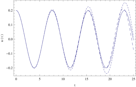
Figure 1: Time variation of $u$ for $\alpha=1.2$, $\beta=3.7$, $\omega=\pi/4$ and $A=0.20$. The solid curve represents the exact numerical solution, the dotted curve depicts the first order Laplace transform approximation, while the dashed curve gives the solution in the second Laplace transform approximation.

VI Conclusions

In the present paper we have considered the possibility of using the Laplace transform and the convolution theorem for solving some nonlinear differential equations. With the use of the Laplace transform nonlinear differential equations can be easily reformulated as integral equations, thus opening the way towards obtaining iterative solutions. As an application of this method we have considered the case of the equation describing the free non-linear vibrations of a uniform cantilever beam. We have reformulated this equation as an integral equation, by using the Laplace transform method, and we have explicitly obtained the first two terms in the iterative expansion of the solution. The comparison with three exact numerical solutions shows that the obtained expressions give a good approximation of the exact solution, at least for small numerical values of $A$. Already the first order approximation, which has a very simple form, can provide a high precision approximation.

Therefore the Laplace transform method of solution of non-linear differential equations may provide a powerful tool for the investigation of the properties of the highly non-linear ordinary differential equations.

References

- (1) M. N. Hamdan and M. H. F. Dado, Large amplitude free vibrations of a uniform cantilever beam carrying an intermediate lumped mass and rotary inertia, Journal of Sound and Vibration, 206 151 (1997).
- (2) M. N. Hamdan, N. H. Shabaneh, On the large amplitude free vibrations of a restrained uniform beam carrying an intermediate lumped mass, Journal of Sound and Vibration, 199 711 (1997).
- (3) J. H. He, Homotopy perturbation method for bifurcation of nonlinear problems, International Journal of Nonlinear Science and Numerical Simulations, 6 207 (2005).
- (4) A. Yildirim, Determination of periodic solutions for nonlinear oscillators with fractional powers by He’s modified Lindstedt-Poincaré method, Meccanica, 45 1 (2010).
- (5) J. I. Ramos, An artificial parameter Linstedt-Poincaré method for oscillators with smooth odd nonlinearities, Chaos, Solitons and Fractals, 41 380 (2009).
- (6) N. Herisanu and V. Marinca, Explicit analytical approximation to large-amplitude non-linear oscillations of a uniform cantilever beam carrying an intermediate lumped mass and rotary inertia, Meccanica, 45 847 (2010).
- (7) M. Akbarzade Y. Khanb, Dynamic model of large amplitude non-linear oscillations arising in the structural engineering: Analytical solutions, Mathematical and Computer Modelling, 55 480 (2012).
- (8) B. S. Wu, C. W. Lim, Y. F. Ma, Analytical approximation to large-amplitude oscillation of a non-linear conservative system, International Journal Nonlinear Mechanics, 38 1037 (2003).
- (9) L. Cveticanin, I. Kovacic, Parametrically excited vibrations of an oscillator with strong cubic negative nonlinearity,Journal of Sound and Vibration, 304 201 (2007).
- (10) A. H. Nayfeh, D. T. Mook, Nonlinear oscillations, Wiley, New York, (1979).
- (11) P. Hagedorn, Nonlinear oscillations, Clarendon, Oxford, (1988).
- (12) A. H. Nayfeh, Introduction to Perturbation Techniques, Wiley, New York, (1993).
- (13) W. P. Wu, P. S. Li, A method for obtaining approximate analytical periods for a class of nonlinear oscillators, Meccanica, 36 167 (2001).
- (14) V. Marinca, N. Herisanu, C. Bota, Application of the variational iteration method to some nonlinear one-dimensional oscillations Meccanica, 43 75 (2008).
- (15) N. Herisanu, V. Marinca, A modified variational iteration method for strongly nonlinear problems, Nonlinear Sci. Lett. A, 1 183 (2010).
- (16) J. H. He, G. C. Wu, F. Austin, The variational iteration method which should be followed, Nonlinear Sci. Lett. A, 1 1 (2010).
- (17) N. Herisanu, V. Marinca, An iterative procedure with application to Van der Pol oscillator, Int. J. Nonlinear Sci. Numer. Simul., 10 353 (2009).
- (18) A. Belendez, et al, An equivalent linearization method for conservative nonlinear oscillators, Int. J. Nonlinear Sci. Numer. Simul., 9 9 (2008).
- (19) J. I. Ramos, Linearized Galerkin and artificial parameter techniques for the determination of periodic solutions of nonlinear oscillators, Appl. Math. Comput., 196 483 (2008).
- (20) A. Belendez, et al, Application of He’s homotopy perturbation method to the Duffing-harmonic oscillator, Int. J. Nonlinear Sci. Numer. Simul., 8 79 (2007).
- (21) J. H. He, Homotopy perturbation method for bifurcation of nonlinear problems, Int. J. Nonlinear Sci. Numer. Simul., 6 207 (2005).
- (22) M. K. Mak, T. Harko, P. C. W. Fung, Viscous fluid cosmological models in Bianchi type I universe, Astrophysics and Space Sci., 249 43 (1997).
- (23) T. Harko, M. K. Mak, Iterative solutions for relativistic dissipative cosmologies, Canadian J. of Physics, 80 591 (2002).
- (24) C. S. J. Pun, et al, Viscous dissipative Chaplygin gas dominated homogenous and isotropic cosmological models, Phys. Rev. D 77, 063528 (2008).
- (25) T. Harko, M. K. Mak, Vacuum solutions of the gravitational field equations in the brane world model, Phys. Rev. D 69 064020 (2004).
- (26) T. Harko, F. S. N. Lobo, and M. K. Mak, A class of exact solutions of the Liénard type ordinary non-linear differential equation, Journal of Engineering Mathematics 89, 193 (2014).
- (27) T. Harko, F. S. N. Lobo, and M. K. Mak, Integrability cases for the anharmonic oscillator equation, Journal of Pure and Applied Mathematics: Advances and Applications 10, 115 (2013).
- (28) N. Teodorescu and V. Olariu, Ordinary and partial differential equations, Vol. I, Editura Tehnica, Bucharest (1978).