Nonclassical States for Non-Hermitian Hamiltonians with the Oscillator Spectrum
Abstract
We show that the standard techniques that are utilized to study the classical like properties of the pure states for Hermitian systems can be adjusted to investigate the classicality of pure states for non-Hermitian systems. The method is applied to the states of complex-valued potentials that are generated by Darboux transformations and can model both non--symmetric and -symmetric oscillators exhibiting real spectra.
1 Introduction
In quantum mechanics one finds two important classes of states of the radiation field: Fock and coherent states. The former, introduced by Fock at the dawn of quantum theory, contain a precise number of photons and produce average fields equal to zero. With exception of the vacuum, the Wigner distribution [1] exhibits negative values in some regions of the phase-space when it is evaluated with the Fock states. Thus, the properties of the quantum states of radiation fields that are occupied by a finite number of photons are far from the Maxwell theory. On the other hand, the coherent states were formally introduced in quantum optics by Glauber [2], although the first antecedents can be traced back to the Schrödinger papers on quantization, see e.g. [3]. They produce average fields different from zero as well as nonnegative symmetrical Wigner distributions. Although the coherent states are constructed as superpositions of Fock states, it is remarkable that their properties are very close to the Maxwell theory. This is because such states satisfy the notion of full coherence introduced by Glauber, while the Fock states (for ) lack second (and higher) order coherence, and thus they are nonclassical. The set of nonclassical states includes also squeezed states [4], even and odd coherent states (also called Schrödinger cats) [5], binomial states [6, 7], photon-added coherent states [8], etc. The difference between the classical and nonclassical properties of a given quantum state is strongly linked to the notion of entanglement [9], which is a fundamental concept required in the development of quantum computation and quantum information [10]. Noticeably, while investigating the quantum properties of a beam splitter, it has been found that the “entanglement of the output states is strongly related to the nonclassicality of the input fields” [11]. That is, the nonclassicality of an arbitrary (input) state can be tested by detecting entanglement in the output of a quantum beam splitter [11, 12].
In the present work we study the nonclassical properties of the states of non-Hermitian Hamiltonians with real spectrum that are generated by Darboux transformations [13, 14]. In general, the systems associated with non-Hermitian Hamiltonians are subject of investigation in many branches of contemporary physics [15]. The applications include the study of unstable (decaying) systems [16], light propagating in materials with complex refractive index [17], -symmetric [18, 19] and -symmetric [20] interactions, multi-photon transition processes [21], diverse measurement techniques [22], and coherent states [3, 23, 24], among others. In the case of the Darboux deformed non-Hermitian systems, the eigenfunctions obey a series of oscillation theorems [25] that permit their study as if they were associated to Hermitian systems. Indeed, the representation space of such non-Hermitian systems can be equipped with a bi-orthogonal structure that provides complete sets of orthonormal states [13]. We shall focus on non-Hermitian oscillators since their bases of eigenfunctions can be used to construct optimized binomial states [26] and generalized coherent states [24], which in turn give rise to a wide diversity of pure states as particular cases. One of the main results reported in this paper is to show that the techniques used to study classical like properties for Hermitian systems can be adjusted to investigate the classicality of the states of Darboux deformed non-Hermitian systems.
The outline of the paper is as follows: In Section 2 we revisit the main properties of the non-Hermitian oscillators we are interested in. The main differences between the conventional orthogonality and the bi-orthogonality are discussed in detail. In Section 3 we introduce the different bi-orthogonal superpositions of states that are to be analyzed, these include the optimized binomial states and diverse forms of generalized coherent states. Section 4 deals with the nonclassicality of the states defined in Section 3. Final comments are given in Section 5. We have added three appendices with relevant information that is used throughout the manuscript concerning operator algebras (Appendix A), and criteria of nonclassicality (Appendix A-2).
2 Non-Hermitian oscillators
The solution to the eigenvalue problem of the dimensionless (mathematical) oscillator is given by the discrete eigenvalues and normalized eigenfunctions
| (1) |
where stands for the Hermite polynomials [27]. Using the linearly independent solutions of the eigenvalue equation and a set of real numbers fulfilling , it can be shown that
| (2) |
is a real-valued function which is free of zeros in , and defines the dimensionless potential
| (3) |
as a Darboux transformation of [13]. Here Erf defines the error function. If , the Hamiltonian is not self-adjoint since is a complex-valued function. Nevertheless, it may be shown that the imaginary part of such potential is continuous in and satisfies the condition of zero total area [25]:
| (4) |
The condition (4) implies a balanced interplay between gain and loss of probability that does not depend on any other symmetry of either or . For instance, besides fulfilling (4), the profile of the real and imaginary parts of the oscillator depicted in Fig. 1(a) is not particularly special (this has been obtained from (3) with , , and ). Looking for concrete symmetries we can take to get even and odd forms of and respectively. The result is a non-Hermitian oscillator which is invariant under -transformations [18]. This case is illustrated in Fig. 1(b) for , and . On the other hand, for , with and positive numbers, the parameter is equal to zero and the expression (3) decouples into the pair of real-valued functions
| (5) |
where the condition must be satisfied to avoid singularities. Fig. 1(c) shows with and . The concomitant corresponds to the specular reflection of . The Hermitian oscillators (5) were first found by Abraham and Moses through the systematic use of the Gelfand-Levitan equation [28], and then recovered by Mielnik as an application of his generalized factorization method [29].
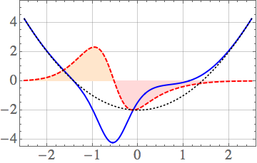
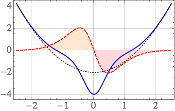
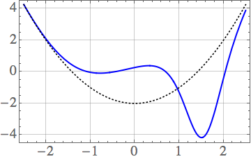
Additionally, the expressions (5) represent a family of systems that converge to the conventional oscillator in the limit . Indeed, it may be verified that
| (6) |
The oscillator is thus a member of the family of complex-valued potentials introduced in (3). This is depicted in the plots of Fig. 1 as a reference.
Fundamental solutions. Another remarkable profile of the complex-valued oscillators (3) is that the functions
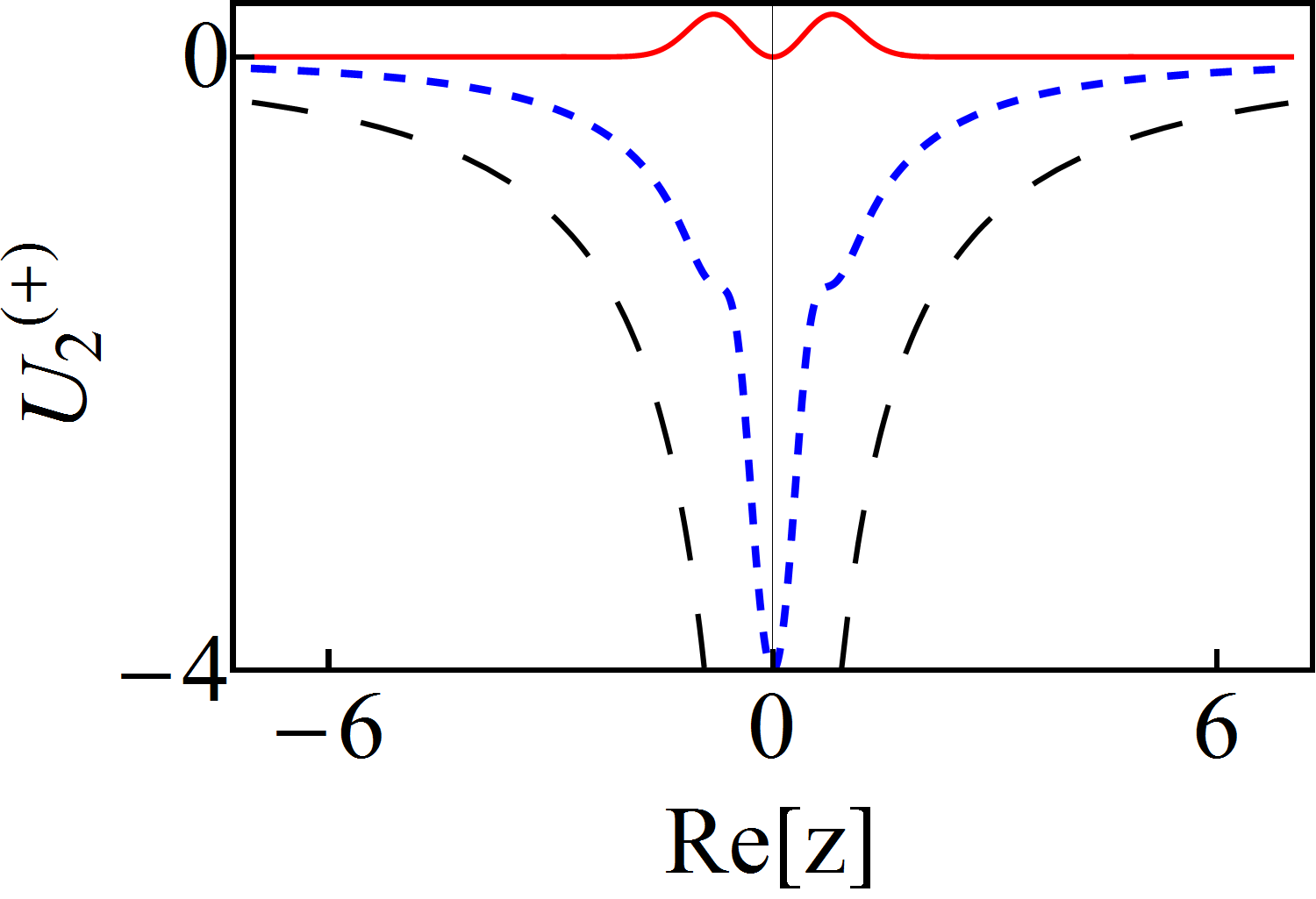
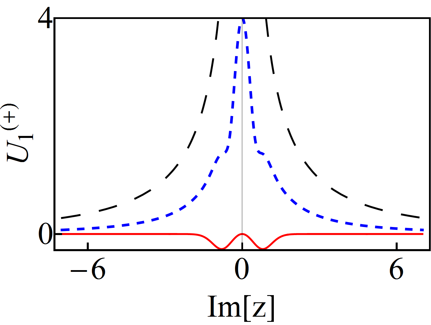
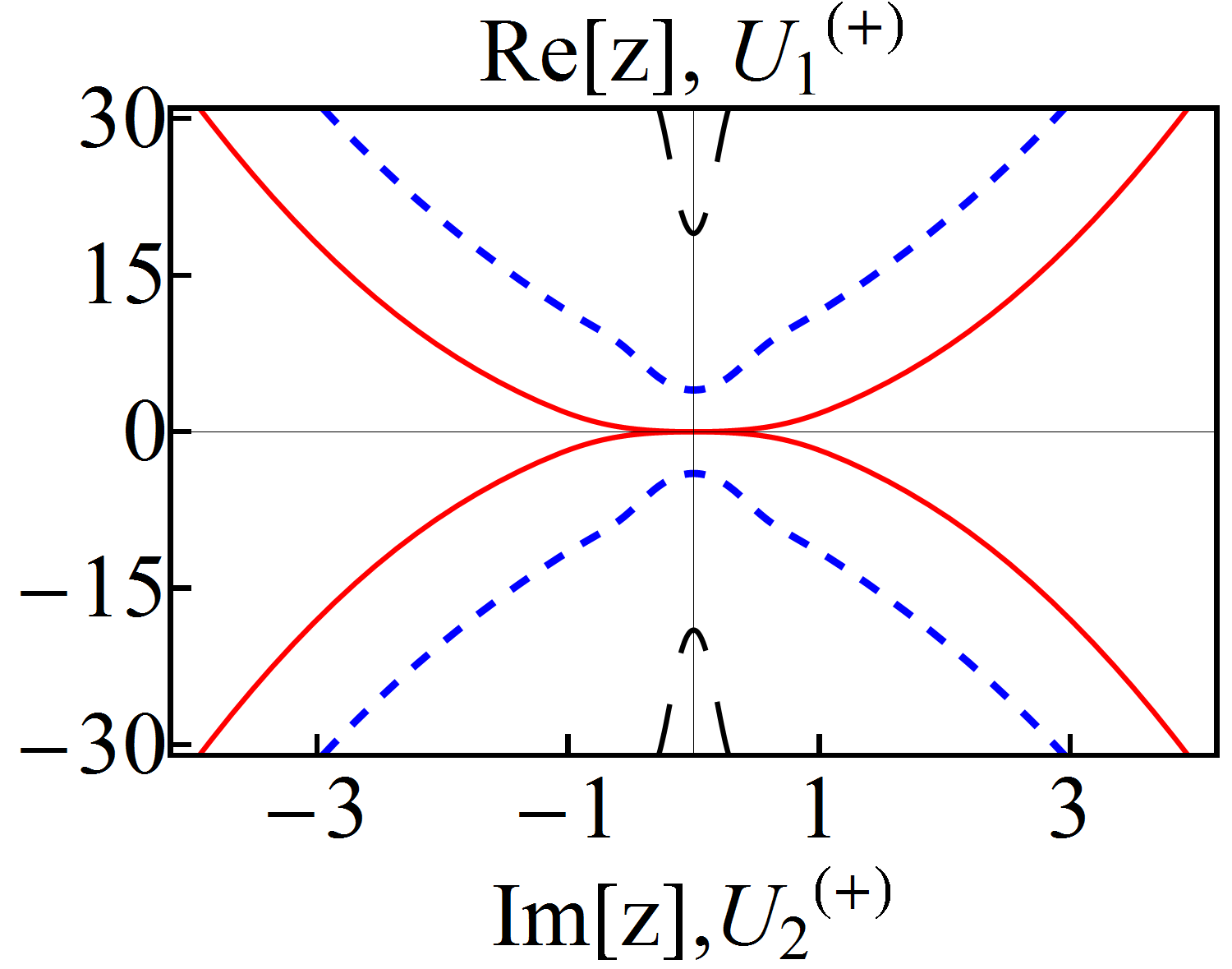
| (7) |
are normalizable solutions of the related eigenvalue equation for . The additional normalizable function
| (8) |
also solves the eigenvalue equation defined by , but it is not derivable from the set and belongs to the energy . The spectrum of the potential is therefore composed of the equidistant energies , .
Bi-orthogonality. Although the functions are normalizable, they form a peculiar set since is orthogonal to all the while the latter are not mutually orthogonal. As a result, in contrast with the Hermitian case, the norm of any superposition of states depends not only on the modulus of the related coefficients but also on the phase shift between them. For instance, the norm of
| (9) |
satisfies
| (10) |
where is the complex-conjugate of . The numbers and are respectively the modulus and argument of the product between and . Thus, depending on the phase-shift , the non-orthogonality of the set produces the oscillations of . The complexity of such a dependence increases with the number of elements in the superposition.
One can face the above difficulties by introducing a bi-orthogonal system (see relevant information in Ref. [24]), formed by the eigenfunctions of and those of its Hermitian-conjugate , written as . The main point is that the bi-product is equal to zero if , and serves to define the bi-norm if .
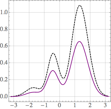
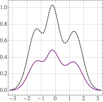
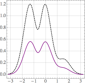
Therefore, besides the conventional normalization , we have at hand the bi-normalization , with for . The bi-norm of the ground state depends on the set [24]. The real and imaginary parts of , as well as the probability density , behave qualitatively equal in both normalizations but their bi-normalized values are usually larger than those obtained with the conventional normalization. Such a difference is reduced as increases. This property is illustrated in Fig. 2 for the first three eigenfunctions , and the corresponding probability densities , of the complex-valued oscillator depicted in Fig. 1(a).
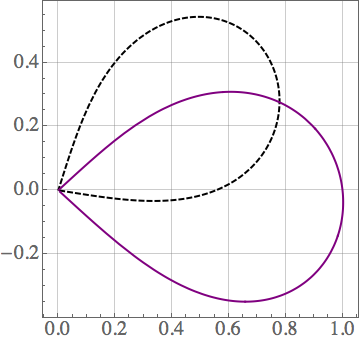
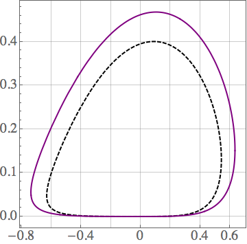
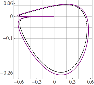
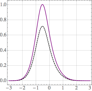
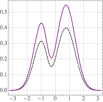
The bi-orthogonal approach avoids the interference produced by the non-orthogonality. For instance, if the sates in (9) are substituted by their bi-normalized versions, we obtain the bi-orthogonal superposition
| (11) |
The bi-norm of the latter state does not depend on the phase-shift
| (12) |
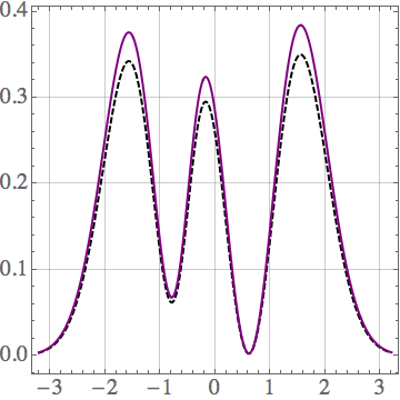
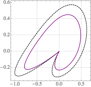
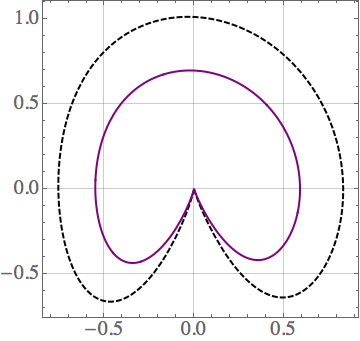
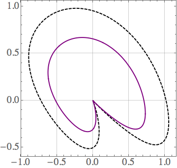
so that is uniquely bi-normalized to 1 by the constant . An additional property of the bi-orthogonal superpositions is that the values of their real and imaginary parts, as well as the values of the corresponding probability densities, are shorter than those obtained from the conventional approach. We show this property in Fig. 3 for the superpositions (9) and (11) with , , , and three different values of the phase-shift . Formally, one may say that and represent two different superpositions of the states and . In the sequel we shall take full advantage of the mathematical simplifications offered by the bi-orthogonal approach.
Operator algebras. It can be shown that there exist at least two different algebras of operators associated with the eigenstates of the complex-valued oscillator [30]. They are generated by two different pairs of ladder operators (see Appendix A for details). The first pair, and , together with the Hamiltonian , satisfy the quadratic polynomial (Heisenberg) algebra
| (13) |
The second pair of ladder operators, denoted by and , together with the Hamiltonian , and an additional operator , satisfy the distorted (Heisenberg) algebra
| (14) |
where is a non-negative parameter that defines the ‘distortion’ suffered by the oscillator algebra when one substitutes the operators , , and for the conventional boson operators, , , and , respectively. The algebras (13) and (14) will serve to the analysis of classicality of the states associated with the complex-valued oscillators (3).
3 Bi-orthogonal superpositions
We shall study the properties of diverse superpositions of states by using
-
(i)
Bi-normalization to obtain regular probability densities.
-
(ii)
Bi-orthogonality to avoid the interference associated with non-orthogonality.
The space of states of , denoted , consists of all the bi-orthogonal superpositions
| (15) |
such that
| (16) |
In turn, denotes the space spanned by the states . The series decomposition of , which is concomitant to in (16), is obtained from (15) by changing . To simplify the notation, hereafter we use no label to denote the bi-orthogonal properties of the system .
The approach we are going to use identifies a threefold partnership between , , and the conventional oscillator , where the eigenvalues play a main role. That is, the triad represents a system for which the energies are threefold degenerate while the energy is only twofold degenerate. In this sense, our model is a generalization of the supersymmetric approach [31] since and are treated as two different faces of the same system, which can be studied in much the same way as in the Hermitian approaches [24].
We are interested in two different classes of superpositions. The optimized superpositions are such that their nonclassicality can be manipulated by tuning the number of elements as well as the state of lowest energy in the sum. The generalized coherent states are constructed in terms of the algebras underlying the complex-valued oscillators (3) and form an over-complete set in . Next, we analyze these classes in detail.
3.1 Optimized binomial states
Let us consider a superposition of adjacent states
| (17) |
where the non-negative integer determines the state of the lowest energy that is included in the packet, and the coefficients give rise to the binomial distribution
| (18) |
That is, the sum (17) is bi-normalized and includes only the eigenstates belonging to the energies . The distribution (18) means that the probability of finding the system in the state is weighted by the probability of having success times in trials. The superpositions (17) are called optimized binomial states [26] since (for ) they converge to the conventional binomial superposition at the oscillator limit.
To investigate the properties of let us take . The modulus of the first coefficient in the expansion is close to 1 and the other coefficients are almost zero. Then, the state is very influential in the behavior of the entire packet since it is weighted by in the superposition. The situation changes if since in this case the modulus of the last coefficient in the sum is close to 1, while the moduli of the other coefficients are almost zero. In such case, is the state of major influence in the packet.
Another important feature of the optimized binomial states is that their mean energy depends on the number which labels the lowest of the involved energies
| (19) |
Considering , we have
| (20) |
That is, is bounded from below by , and from above by and . Fixing and in (19) we can write
| (21) |
Then, from (18) we arrive at the Poisson distribution:
| (22) |
In this form, as a limit version of the optimized binomial state , we introduce the optimized Poisson state
| (23) |
In the quantum oscillator limit (6), the superposition (23) acquires the form
| (24) |
which coincides with the conventional coherent state for , see Eq. (B-25) of Appendix A-2.
3.2 Generalized coherent states
The ground state is annihilated by both pairs of ladder operators , , and , , see Appendix A. In any case we can construct coherent states as eigenstates of the respective annihilator operator. We write
| (25) |
The super-index stands for natural (), distorted (), natural displaced (), and distorted displaced (). Such nomenclature refers to the form in which the coefficients have been selected, as it is explained below. For simplicity, we use Dirac notation.
If the superposition (25) is an eigenvector of the natural annihilation operator with complex eigenvalue , then it is a natural coherent state [24]. We write111A factor of the complex eigenvalue reported in [24] has been absorbed in .
| (26) |
Notice that also the ground state is eigenvector of , but its complex eigenvalue is equal to zero. Moreover, as , we see that the eigenvalue is twice degenerate. The straightforward calculation shows that the vectors and minimize the uncertainty relation (A-9). In this sense and represent two different types of minimal uncertainty states.
Similarly, the distorted coherent states [24] are defined as eigenvectors of the distorted annihilation operator with complex eigenvalue . In this case we write
| (27) |
with being the Pochhammer symbol [27]. The eigenvalue is also twice degenerate because and are annihilated by . As and minimize the uncertainty relation (A-16), they represent two different types of minimal uncertainty states.
Another interesting superposition (25) is obtained by demanding that the vector be the displaced version of a fiducial state. The states and are invariant under the action of the operator exponentiations and , because they are annihilated by both operators and . The latter means that and can be used as fiducial states. Considering the operators
| (28) |
one has the ‘displaced’ states and . Remark that the ground state is invariant under the action of and , so it is also a displaced state.
In the rest of this work we shall omit the description of the states since their properties are qualitatively similar to those of the (distorted) displaced coherent states:
| (29) |
In contrast to the previous superpositions, the states do not minimize the uncertainty relation (A-16) for arbitrary values of , but only for . The latter means that and are the only displaced coherent states of minimal uncertainty.
4 Nonclassical states for non-Hermitian oscillators
The -representation introduced by Glauber [32] and Sudarshan [33] defines a limit for the classical description of radiation fields. If the -function is not accurately interpretable as a probability distribution then the field “will have no classical analog” [2]. This notion of nonclassicality applies immediately to the Fock states for because their -functions are as singular as the derivatives of the delta function , and are negative in some regions of the complex -plane. The latter means that the light beams represented by any of the Fock states cannot be described in terms of the electrodynamics introduced by Maxwell. In turn, the Glauber states [2], usually denoted , are classical because their -function is precisely . The vacuum is also classical as it is a coherent state with complex eigenvalue equal to zero. In general, the states for which the quadrature variances obey the inequalities
| (30) |
admit a non-negative -function [2]. Here, stands for the variance of the operator . If either of the inequalities (30) is not satisfied, the -function is ill-defined and the state is called squeezed [34, 35, 4]. In these cases it is better to represent the state using the Wigner distribution [1], which is regular and always exists. Nonclassical states have Wigner functions which either are negative in some regions of the phase-space or are squeezed in one of the variables of the phase-space.
In modern days, the nonclassicality of a state can be tested by another excellent method, which follows from the use of the quantum beam splitter. It creates entangled states at its output ports while at least one of its inputs are fed with a nonclassical state. The device is used frequently both in theory and experiment, since it not only tests the nonclassicality of the state, but also quantifies the degree of nonclassicality in an efficient way [12, 11]. There are some well-known nonclassical states in the literature, which include squeezed states [4], even and odd coherent states (also called Schrödinger cats) [5], binomial states [6, 7], photon-added coherent states [8], etc. Apart from the nonclassical states that arise from the harmonic oscillator, there exist many other such states emerging from different generalizations of coherent states; see, for instance [36]. Other interesting nonclassical states have also been shown to originate from some mathematical frameworks, in particular, from the noncommutative systems reported in [37, 38, 39]. The striking feature of such systems is that they give rise to well-defined nonclassical states although the corresponding models are non-Hermitian.
Quite recently it has been shown that the appropriate generalizations of the oscillator algebra permit the construction of nonlinear coherent states that satisfy a closure relation which is expressed uniquely in terms of the Meijer -function [40]. This property automatically defines the delta distribution as the corresponding -representation. However, in the same work, it is also shown that does not exist a classical analog for such states since they lack second-order coherence and exhibit antibunching. Thus, although their -representation is a delta function, the nonlinear coherent states studied in [40] are not classical since they are not fully coherent in the sense established by Glauber [2]. Similar results have been obtained for the para-Bose oscillator [41, 42]. The algebras (13) and (14) that we have used to construct the coherent states of Section 3.2 satisfy the requirements established in [40]. Considering also that the bi-orthogonality permits to operate the non-Hermitian oscillators as in the conventional Hermitian case, it may be shown that the corresponding -representation is proportional to the delta distribution. Nevertheless, the latter means the existence of a classical analog only if the states of Section 3.2 are fully coherent.
Instead of investigating whether our coherent states lack second (or higher) order coherence, we shall use some of the techniques described in Appendix A-2 to study their classicalness. Namely, we are going to study the corresponding variances, Mandel parameter, Wigner distribution and purity.
4.1 Nonclassical optimized binomial states
Let us investigate the properties of the distorted quadratures (A-15) in terms of the optimized binomial states (17)-(18). The variances and may be expressed in the form (B-17) of Appendix A-2:
| (31) |
where we have used (A-16) and . The straightforward calculation gives and , with
| (32) | |||
| (33) |
In the above expressions , and . Hereafter we make in .
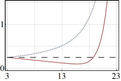
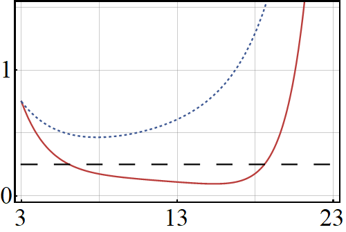
It may be shown that there is always a subset of the mean energies (19)-(20) for which . Thus, it is always possible to find a mean energy producing the squeezing of the distorted quadrature . The latter is illustrated in Fig. 4 for , and two different values of . In turn, the squeezing of occurs for only, and it is not as strong as the one suffered by since is just slightly larger than . In general, the optimized binomial states (17) are of minimal uncertainty (i.e., they are classical states) only at the lowest mean energy for either (i) and any value of , or (ii) and .
In the quantum oscillator limit (6) one has
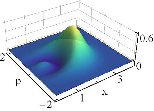
| (34) |
Clearly, we recover the conventional binomial state for . This state is squeezed in the quadrature , for and , as shown in the Wigner distribution of Fig. 5(a). If , besides the squeezing of , the Wigner distribution exhibits negative values in different zones of the phase-space, see Figs. 5(b) and 5(c). The latter results confirm that the optimized binomial states (34) are stronger nonclassical than the conventional ones.
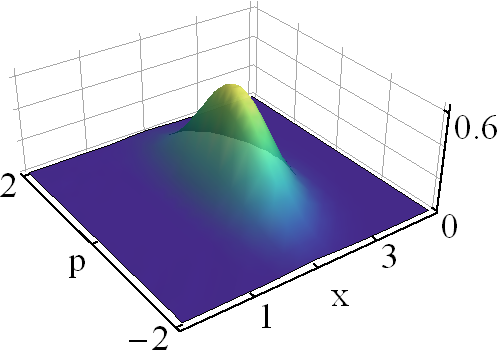
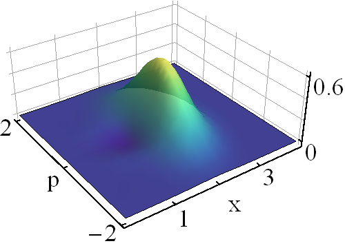
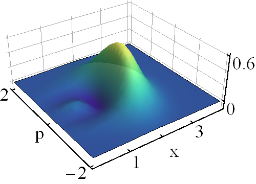
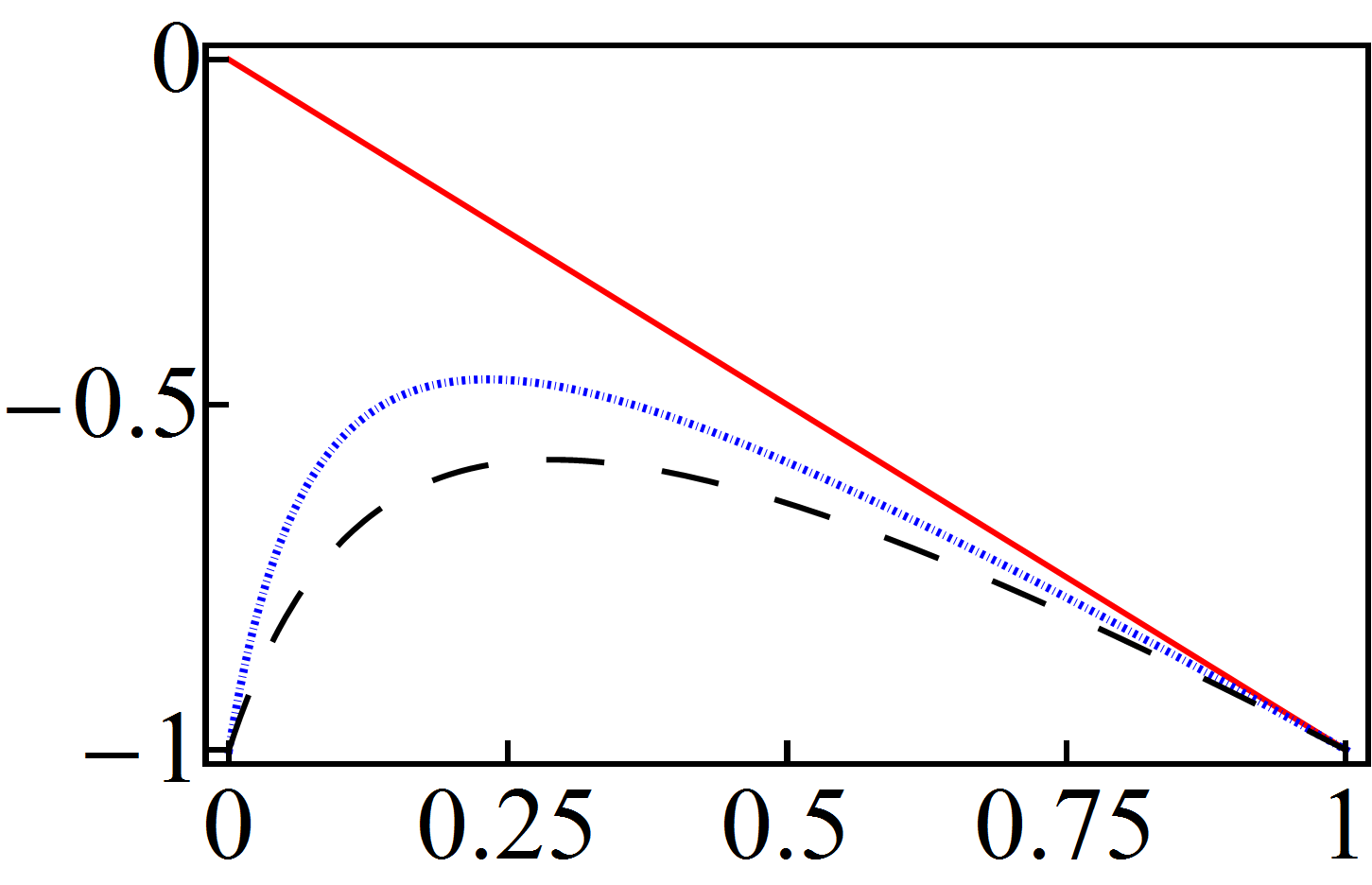
To get more insights about the optimized binomial states (34) we have depicted the related Mandel parameter , as a function of , in Fig. 6. For the superposition (17) is reduced to the state , so that all the curves shown in Fig. 6 converge to as . In turn, for , all the curves take the value at since only the Fock state is included in the sum. Thus, for and any , the Mandel parameter in this case is always negative. Then, the optimized binomial states (34) are sub-Poissonian for , and thus do not admit any classical description.
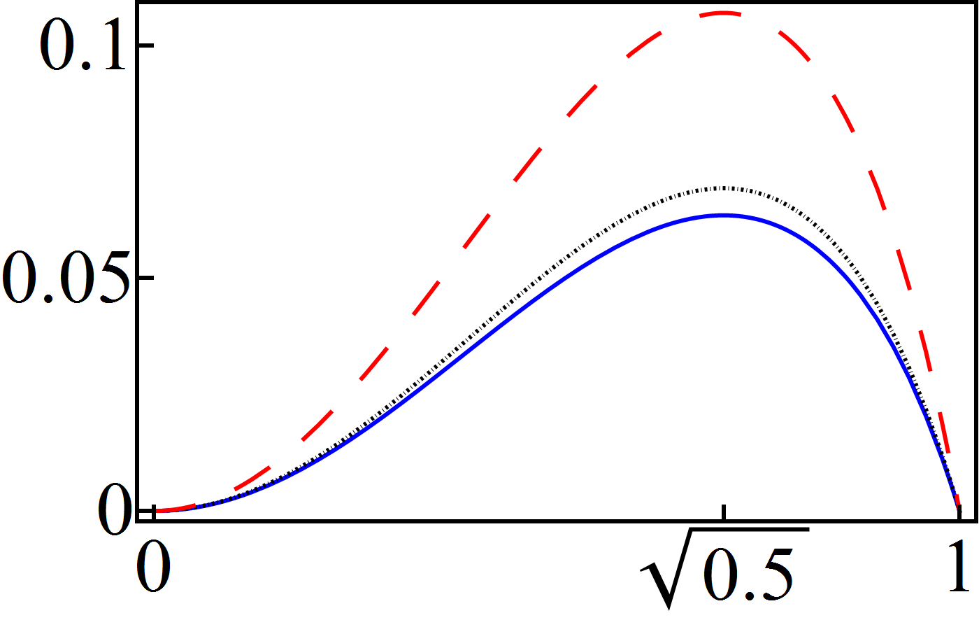
Let us apply also the beam-splitter technique (see Appendix A-2) to the states we are dealing with. We may study the purity (linear entropy) in terms of either the transmission coefficient of the beam-splitter or the probability that defines the superposition (34). In the former case it is convenient to fix and to parameterize the purity with and . Then one finds that the purity is equal to zero for and , see Fig. 7. However, it is important to remark that such results give no special information since they correspond to complete reflectance (i.e., the beam-splitter is indeed a perfect mirror) and complete transparency (no beam-splitter), so the output is respectively the vacuum and the state which was injected in input. In general, for other values of , the purity reaches its maximum at , i.e., when the testing beam-splitter is .
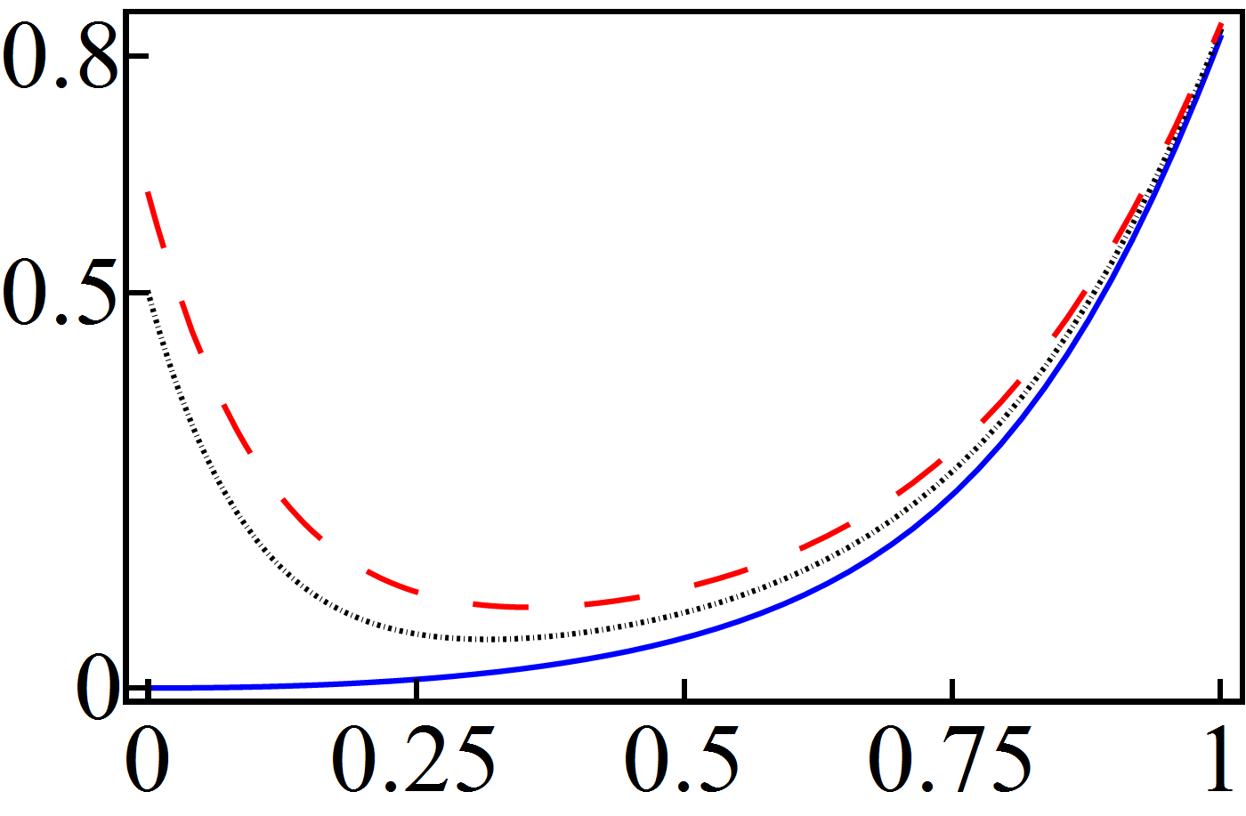
To analyze in terms of the probability we must fix and . Then, with exception of the purity for , we find for any value of (see Fig. 8). The latter confirms, once again, that the optimized binomial states are nonclassical. Concerning the case , the purity is equal to zero at only. Thus, the superposition (34) only includes the vacuum state , which is clearly classical.
4.1.1 Nonclassical optimized Poisson states
It may be shown that the optimized Poisson states (23) are minimum uncertainty states for concrete values of the parameters like either , or . In any case, they become states of minimum uncertainty as . For other values of the parameters either or is squeezed, see Fig. 9.
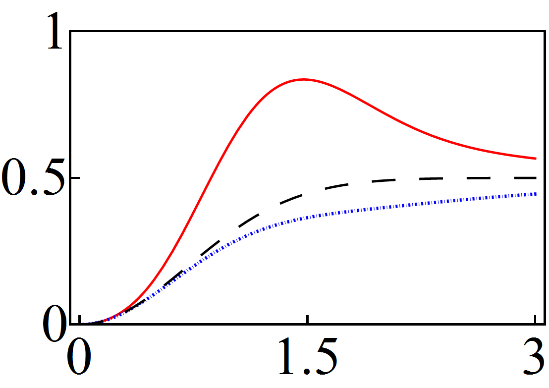
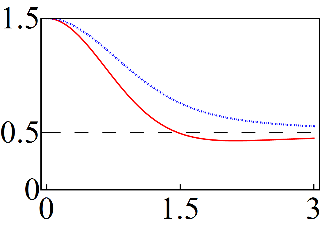
In the quantum oscillator limit (6), the superposition (23) acquires the form of Eq. (24). As indicated above, for this state is reduced to the conventional coherent state, so that the Mandel parameter is equal to zero, as expected. For other values of , the optimized Poisson states (24) are sub-Poissonian. In fact, in Fig. 10 we see that the Mandel parameter becomes zero as , and it is equal to for at (i.e. at the lowest mean energy ). In other words, for and finite values of , the optimized Poisson states are nonclassical.
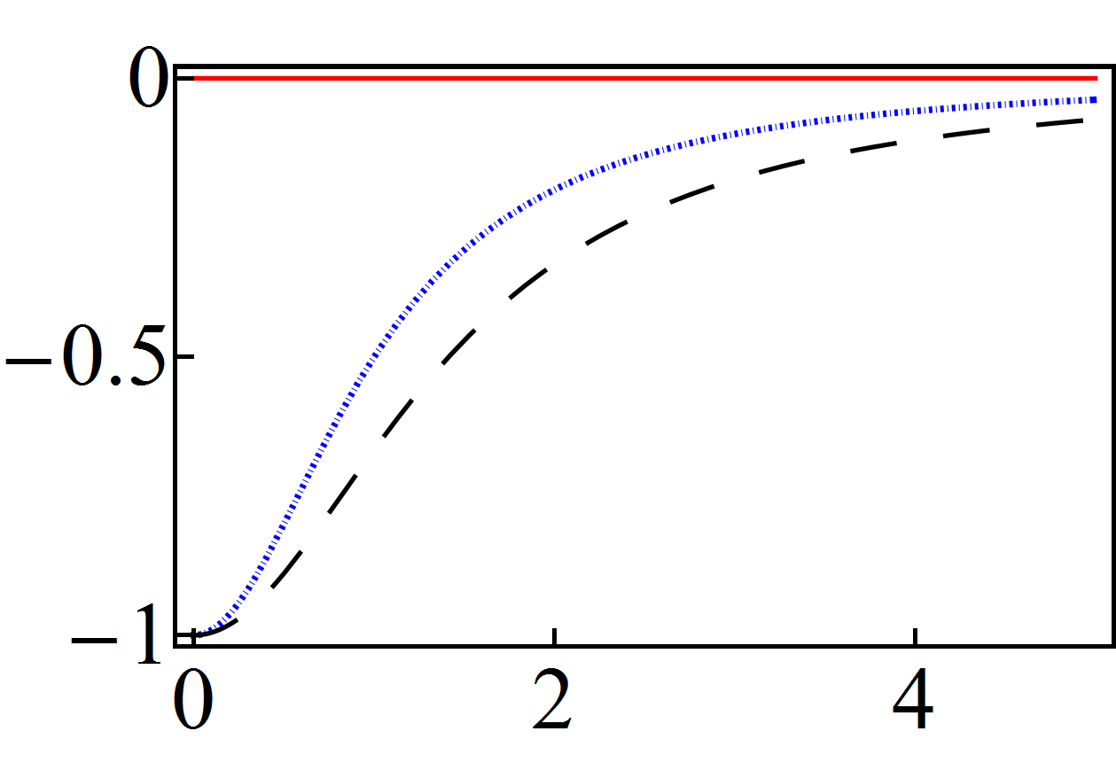
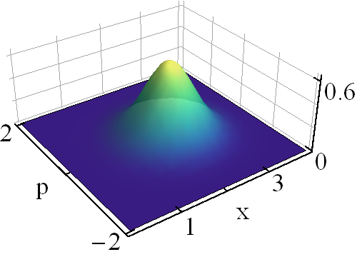
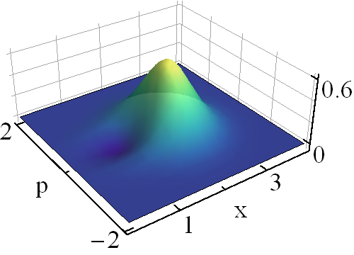
For completeness, we show the Wigner function of in Fig. 11. Clearly, for one has a conventional (classical) coherent state. Other values of give rise to both, the squeezing of and the negativity of the Wigner function in some regions of the phase-space.
Photon added coherent states. The expression (24) resembles the structure of the photon-added coherent states for the conventional harmonic oscillator [8], written in Dirac notation as
| (35) |
In both cases the superpositions are infinite and start with the eigenstate . The main difference lies on the coefficients, for if we make , then
| (36) |
If we see that, up to the normalization constant , the coefficients are the same. For other values of the superpositions (24) and (35) are different in general.
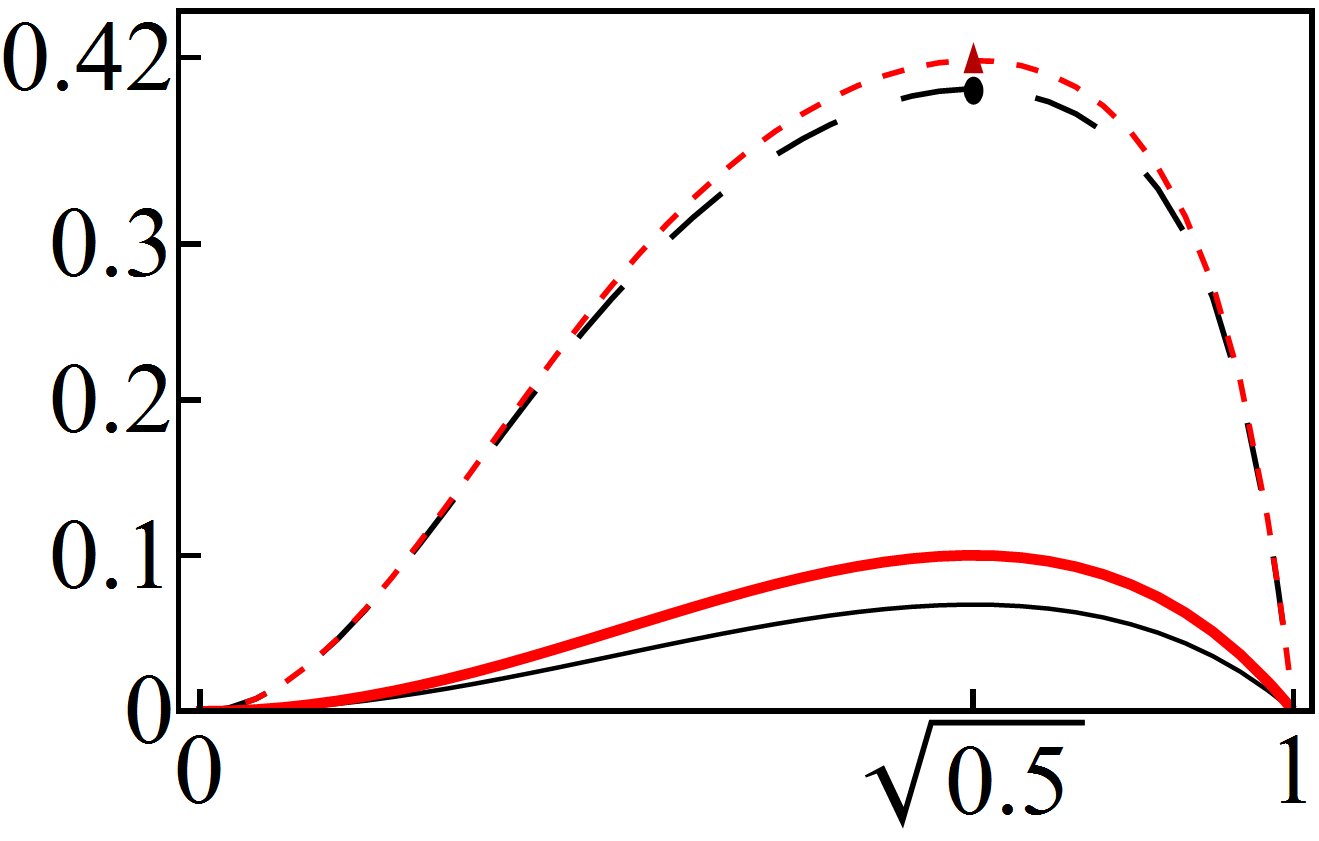
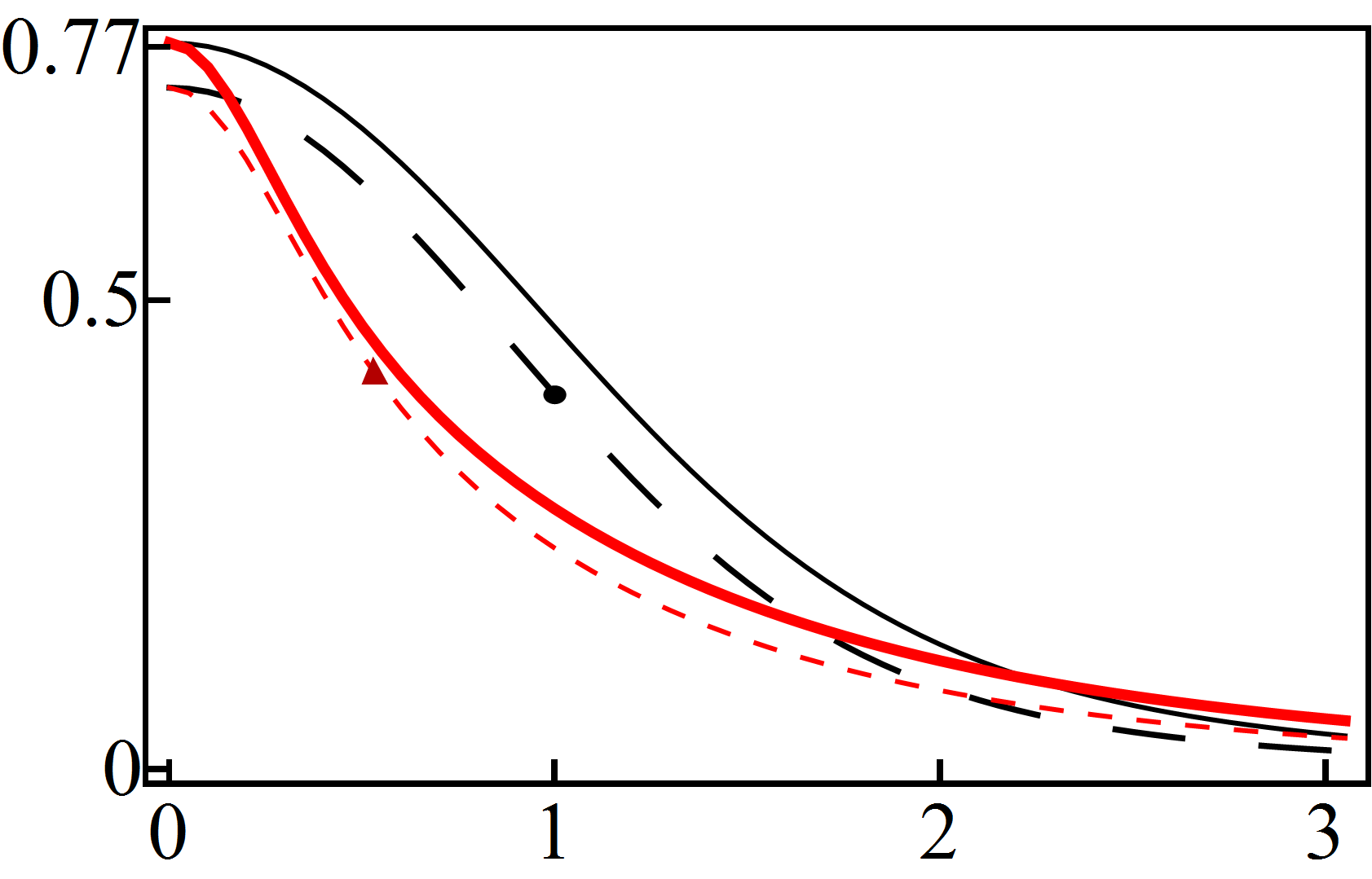
Let us compare with in order to identify which one is stronger nonclassical. Using the beam-splitter technique, we find that the nonclassicality of these states depends on different parameters. For instance, in Fig. 12(a) we have fixed the value of the mean energy as and, after adjusting the parameters , , and , the purities and have been depicted in terms of the transmission coefficient . As a global property, we see that the purity is maximum at in all the cases. Besides, we can appreciate that . Thus, for the parameters used in the figure the state is stronger nonclassical than . The situation changes if we fix , and adjust the other parameters to plot the purity in terms of . Then holds for small values of and , and is valid for large values of such parameters. The latter is illustrated in Fig. 12(b) for and .
4.2 Nonclassical natural coherent states
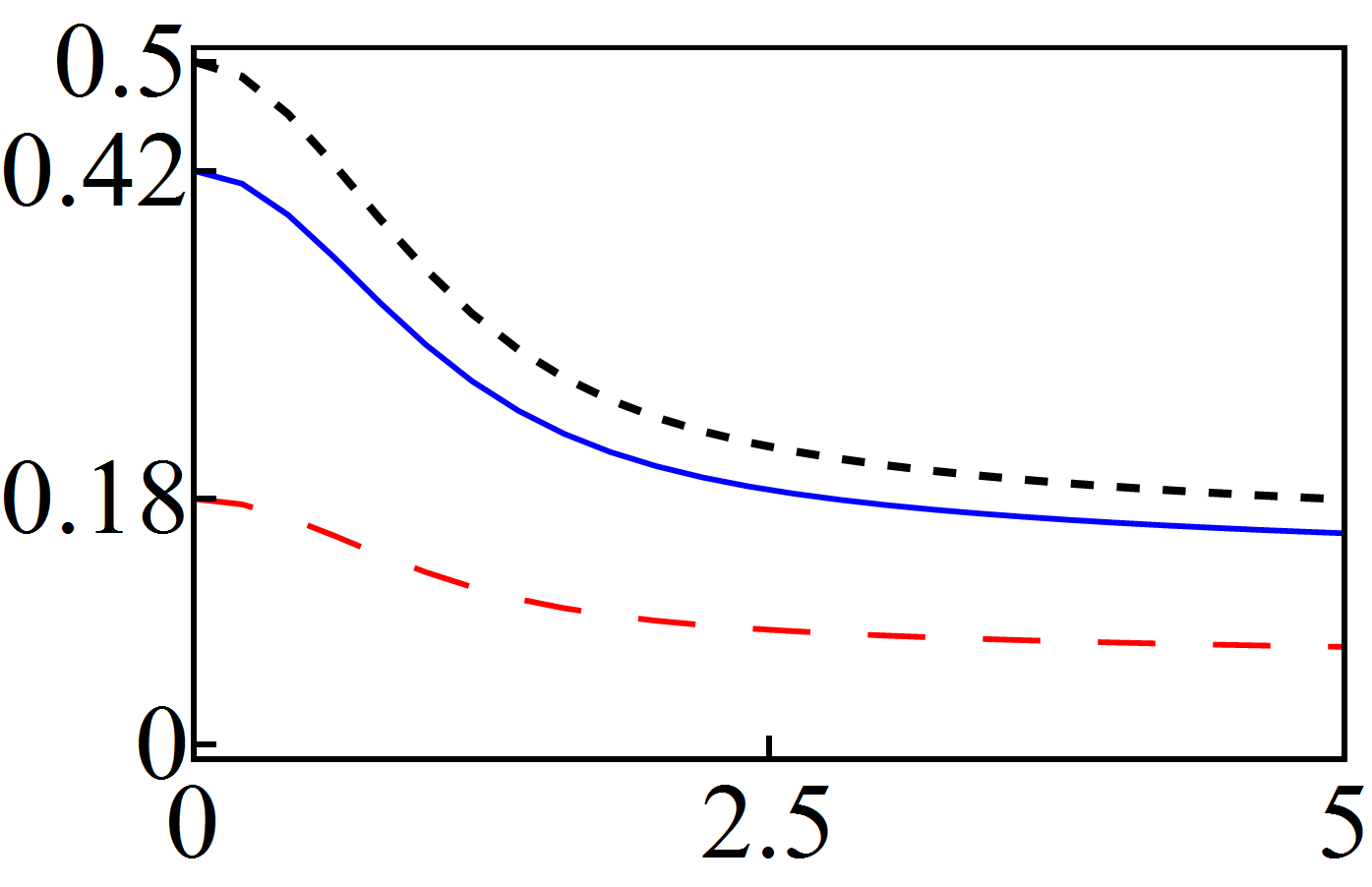
By construction, the natural coherent states minimize the uncertainty relation (A-9) of Appendix A to investigate their properties in the oscillator limit (6), we first calculate the purity using Eq. (B-23) of Appendix A-2 with , , and in the Fock basis . The result is depicted in Fig. 13(a). As we can see, this function is always different from zero and decreases as for any value of the transmission coefficient . That is, the states are nonclassical. The latter is confirmed by noticing that the Mandel parameter is always negative, as it is shown in Fig. 13(b).
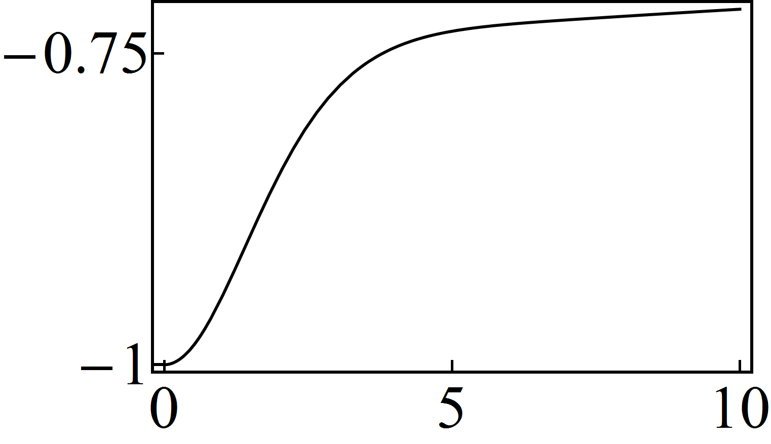
On the other hand, the variances of the physical quadratures and can be expressed in the form (B-17) of Appendix A-2, with , , and
| (37) |
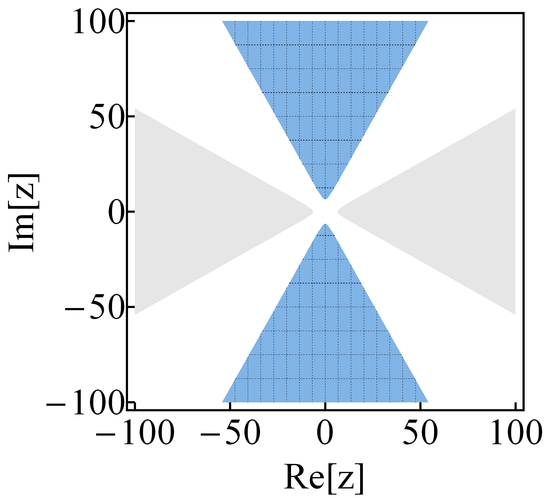
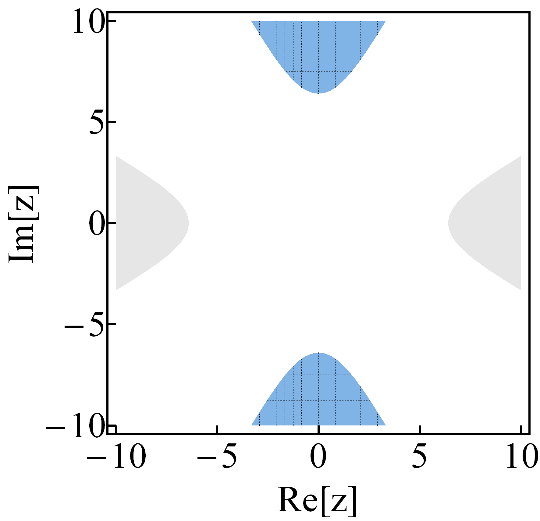
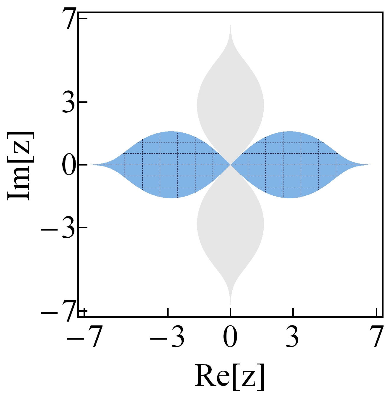
In Fig. 14, we show the regions of the complex -plane where the squeezing of either (grey zones) or (mesh, dashed blue zones) occurs. Notice that the squeezing is maximum at the phase values , and , respectively. The white zones are the regions of no-squeezing, they overrun four distinguishable areas defined along the phase values , , and a circle of radius that is centered at the origin. Comparing the Figs. 13 and 14, we see that the purity and the Mandel parameter give information that is complementary to that obtained from the variances of the quadratures. Namely, and indicate strong nonclassicality for the states that satisfy the condition , where no squeezing is expected for neither nor .
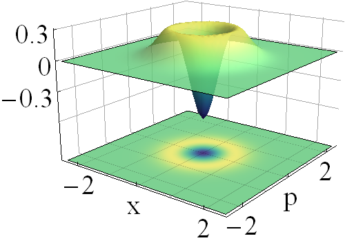
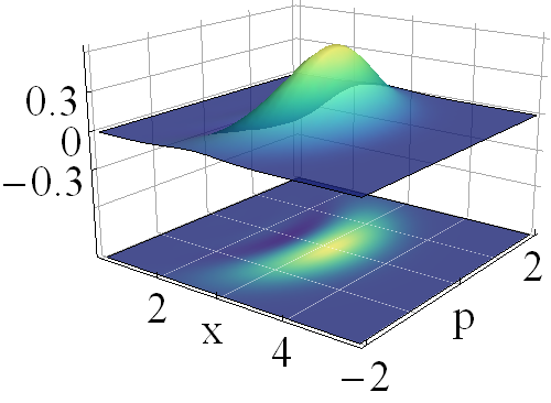
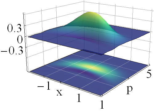
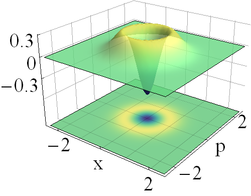
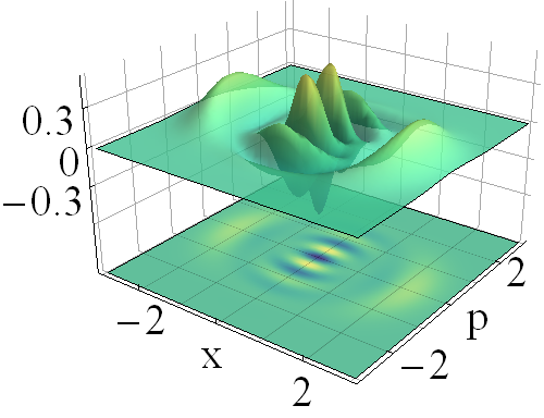
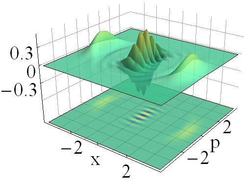
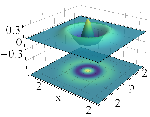
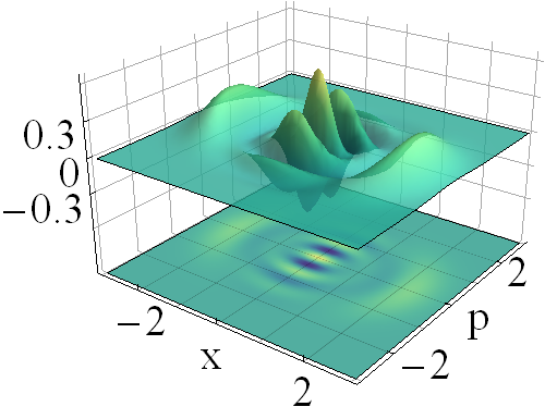
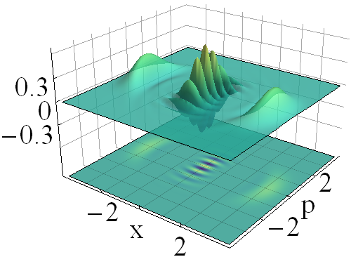
In Fig. 15 we show the density plots of the Wigner function of for different values of . In particular, for the natural coherent state is nonclassical because it coincides with the first excited state of the oscillator , as shown in Fig. 15(a). If and the quadrature is squeezed; this is illustrated in Fig. 15(b) with . In turn, for one has the opposite result, is squeezed; see Fig. 15(c).
4.2.1 Even and odd natural coherent states
We can use the natural coherent states (26) to construct additional nonclassical states. Following [5] we introduce the vectors
| (38) |
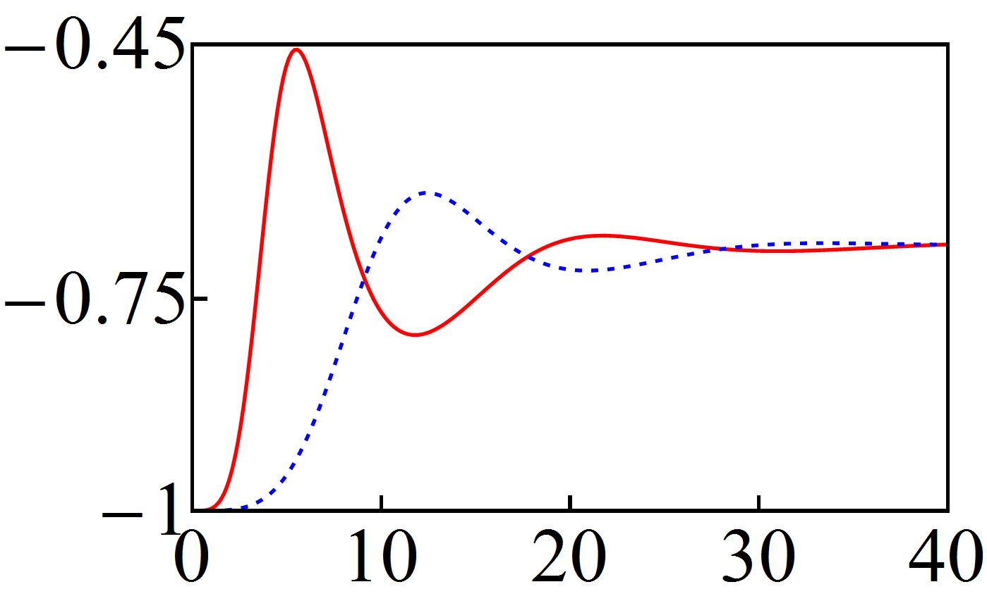
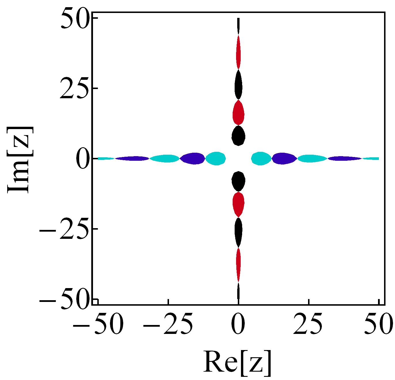
and call them even and odd natural cat states, respectively. The related Mandel parameter is always negative, see Fig. 16(a), so that are nonclassical. The variances of the natural quadratures (A-8) can be expressed in the form (B-17) of Appendix A-2, with , , and
| (39) |
In this case the quadratures are squeezed in very localized regions that are distributed along the real and imaginary axes of the complex -plane. This is illustrated in Fig. 16(b), where we can appreciate a ‘discretization’ of the eigenvalue as follows. The quadrature is maximally squeezed along the real axis, in intervals that are defined by the points , , with , and denoting either even () or odd (). For odd natural cats we make , with defining the green zones that are closest to the origin in Fig. 16(b). For the even natural cats we write , with defining the blue zones that are closest to the origin in the same figure. The intersection of the above intervals is empty, and they are such that the points interlace. That is . The phases constraining the green and blue zones are defined in intervals , with , that are shorter as increases. A similar description holds for the squeezing of along the imaginary axis.
In the oscillator limit (6), the natural cat states preserve their nonclassicality. In Fig. 17 the Wigner function becomes negative in diverse zones of the complex -plane. Such regions are less evident for .
4.3 Nonclassical distorted coherent states
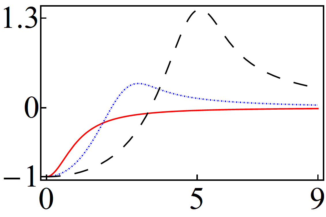
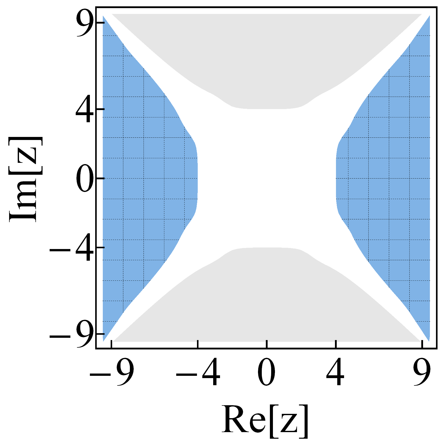
By construction, the distorted coherent states are minimal uncertainty states with respect to the uncertainty relation (A-16). In the oscillator limit, the Mandel parameter depends on the parameter of distortion. In Fig. 18(a), we see that the states are sub-Poissonian for any value of whenever . For arbitrary values of , they are nonclassical only in the interval . Here the value of is defined by : it is larger if the value of is increased.
The variances of the physical quadratures and can be expressed in the form given by Eq. (B-17) of Appendix A-2, with , , and
| (40) | |||
where
| (41) |
For , the quadratures and are squeezed along the real and imaginary axes, respectively. However, for larger values of , they are squeezed along the imaginary and real axes. Thus, for the squeezing is rotated by , as shown in Fig. 18(b).
4.3.1 Even and odd distorted coherent states
For the even and odd distorted cats
| (42) |
the variances of the distorted quadratures (A-15) can be expressed in the form given by Eq. (B-17) of Appendix A-2, with , , and
| (43) |
In Fig. 19, we show the regions of the complex -plane where and are squeezed for the even distorted cat with the indicated value of . Depending on the phase , the squeezing is present in zones defined by the interval and aligned with either the real or the imaginary axes. Such zones are of maximum width at and are slenderer as either or .
In the oscillator limit (6), the variances of and are calculated using the Eq. (B-17) of Appendix A-2, with
| (44) | |||
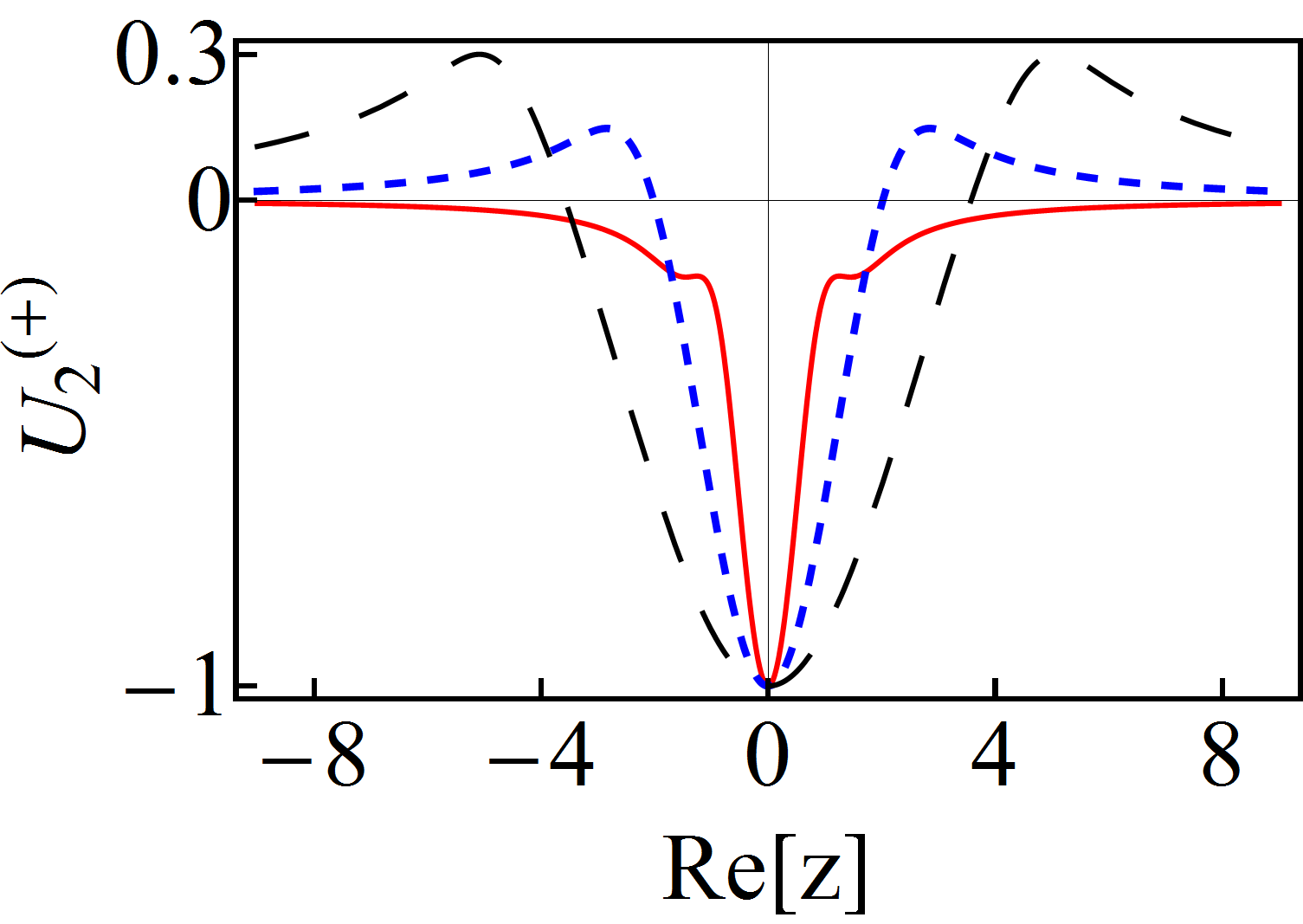
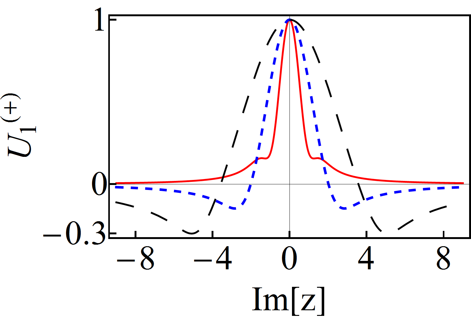
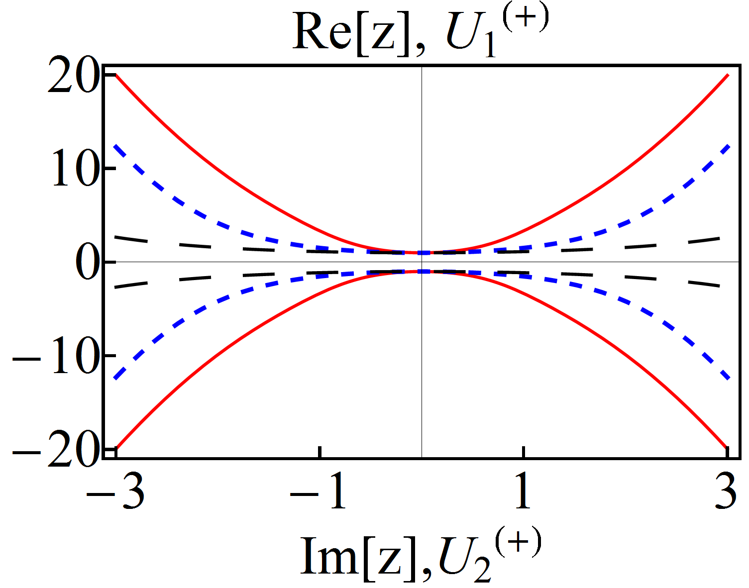
and given in (41). The quadratures and are squeezed in narrow zones of the complex -plane that are defined along the real and imaginary axis, respectively. As in the previous cases, there is no squeezing for small values of . Moreover, the squeezing regions are slenderer as . To illustrate the phenomenon, in Fig. 20 we show the behavior of the -functions that define the variances and of the even distorted cat . As is positive definite along the real axis, see Fig. 20(c), the quadrature is squeezed in the intervals of the real axis where the function is non-negative. The latter can be identified in Fig. 20(a). Similarly, from Fig. 20(c) we see that is negative along the imaginary axis. Then, is squeezed in the intervals of the imaginary axis for which is negative, see Fig. 20(b).
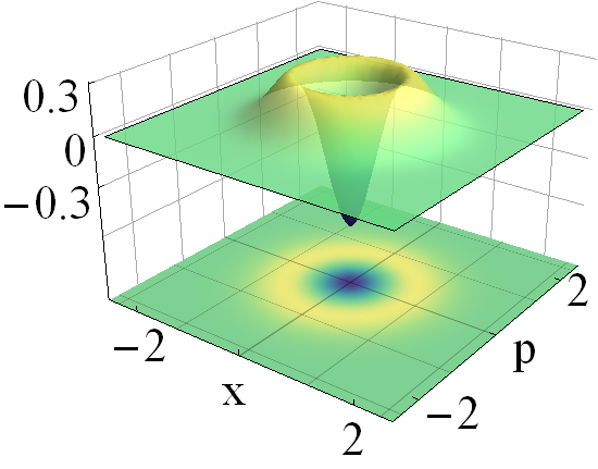
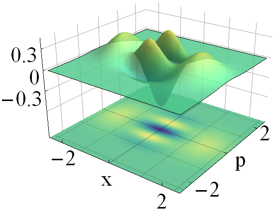
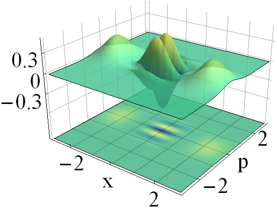
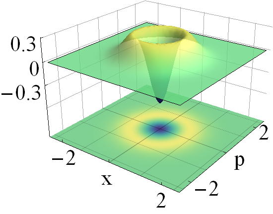
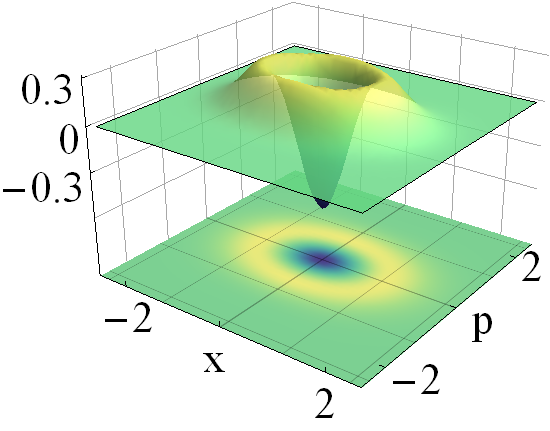
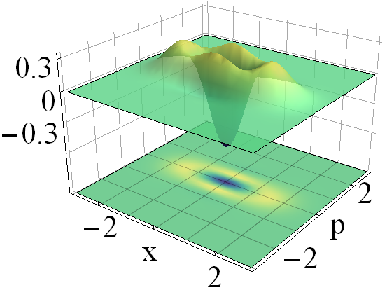
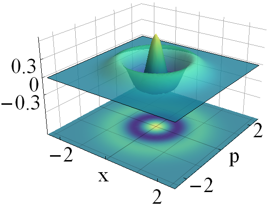
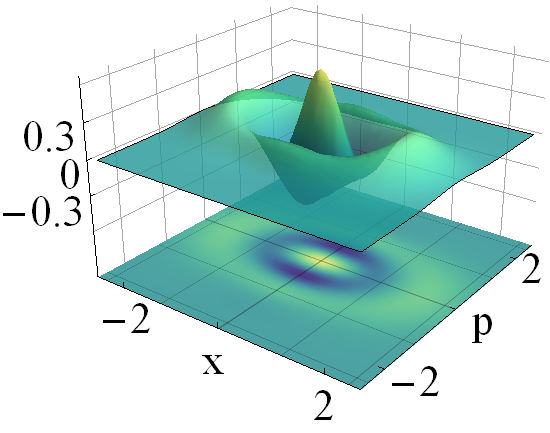
In Figs. 21 and 22 we show the density plot of the Wigner distribution of the even and odd cat states (42), respectively. In both cases we have used for , , and different values of . The Wigner distribution is negative in different regions of the complex -plane, and it exhibits oscillations as increases. The distortion parameter is used to control such oscillations by reducing their number as increases.
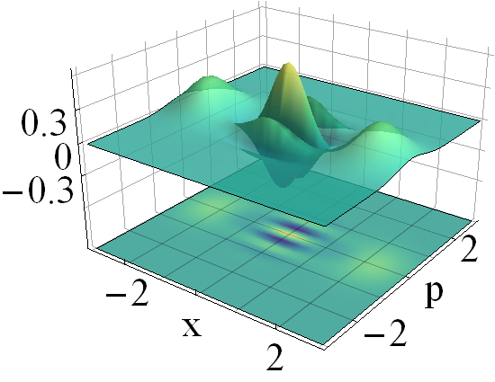
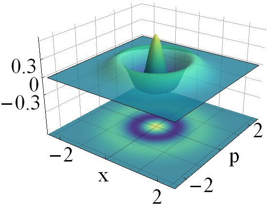
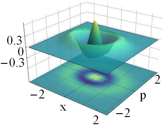
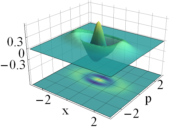
On the other hand, the straightforward calculation shows that neither nor are squeezed for the odd distorted cats . The same holds for the physical quadratures and , evaluated in the oscillator limit state .
4.4 Nonclassical displaced coherent states
Let us analyze the properties of the displaced coherent states and introduced in (29). In the oscillator limit, the variances of the physical quadratures and are derived from Eq. (B-17) of Appendix A-2, with
| (45) | |||
and
| (46) | ||||
The squeezing of and for is quite similar to that obtained for the distorted coherent states of the previous section.
On the other hand, for the even and odd displaced coherent states
| (47) |
the variances of the distorted quadratures (A-15) are calculated from Eq. (B-17) of Appendix A-2, with
and given in (46). From Fig. 23 we see that, along the real axis, the function is positive definite for any while is non-negative for only. Similarly, along the imaginary axis, is always negative but only for the function is negative. The conclusion is that only for we obtain the squeezing of either or . Remarkably, for this value of the parameter of distortion, the distorted and the displaced coherent states coincide.
5 Conclusions
We have studied the nonclassical properties of some pure states of the non-Hermitian Hamiltonians with real spectrum that are generated by Darboux (supersymmetric) transformations. Our interest has been focused on non-Hermitian oscillators since their eigenfunctions form bi-orthogonal bases of states in a straightforward form [24]. Depending on the parameters that define the Darboux transformation, these oscillators may be either parity-time-symmetric or non-parity-time-symmetric [13]. The pure states studied in this work are constructed as superpositions of the related bi-orthogonal basis, they include the so-called optimized Binomial and optimized Poisson states [26, 30], together with the even and odd versions of the generalized coherent states that are associated with the dynamical algebras of the non-Hermitian oscillators [24, 30].
One of the main results reported in this paper is to show that the techniques used to study classical like properties for Hermitian systems can be adjusted to investigate the classicality of the states of non-Hermitian systems. The latter is relevant considering that, although the non-Hermitian systems are widely used in contemporary physics [16, 17, 18, 19, 20, 21, 22], the classicality of the related quantum states is rarely studied. The main difficulty is that non-Hermiticity of a given operator implies that the orthonormal properties of the related eigenfunctions are not granted a priori. Since most of the approaches implemented to analyze classicality assume orthonormality of states, it is not clear how to translate such methods to the non-Hermitian case in general. Such a difficulty can be overpassed by considering a bi-orthogonal basis for the space of states of the non-Hermitian system, just as we have shown throughout this work. It is expected that our approach can be applied in the study of resonances [16] (where the non-Hermiticity of the Hamiltonian defining the interaction of a scatterer with a projectile leads to the temporal trapping of the later by the former) and in the propagation of light in materials with complex refractive index [17] (where the imaginary part of the refractive index may model absorption or amplification of electromagnetic signals).
Concerning the non-Hermitian oscillators we have shown that the corresponding bi-orthogonal bases converge to the Fock basis in the appropriate limit (i.e., after canceling the imaginary part of the potential and properly selecting the parameters), so that the bi-orthogonal superpositions of such states are reduced to pure states of the conventional harmonic oscillator. In particular, we have found that the generalized coherent states of the non-Hermitian oscillators are not minimum uncertainty states for the physical position and momentum quadratures in the oscillator limit. Nevertheless, they exhibit some interesting nonclassical behavior. For instance, depending on the module and complex-phase of the coherence parameter , the physical quadratures can be squeezed for the class of generalized coherent states that we have called “natural” (see Section 3.2). The squeezing is clearly exhibited in the corresponding Wigner distribution and revealed by the Mandel parameter for which it is shown that the photon number distribution is sub-Poissonian. The other class of generalized coherent states, called “distorted”, have similar quadrature squeezing properties. However, the Mandel parameter reveals a different behavior since the photon distribution becomes sub-Poissonian for some values of , but it converges to a Poissonian distribution at the limit . The latter implies a nonclassical-to-classical transition for the distorted coherent states (see [8] for the results on the matter for photon-added coherent states). Such a transition can be also manipulated with the parameter that defines the related dynamical algebra.
Our method can be extended to construct and study intelligent states associated with the dynamical algebras of the non-Hermitian oscillators. The model involves finite difference equations, which deserve special treatment. Work in this direction is in progress.
Appendix A Operator algebras
The properties of the algebras used throughout this work are summarized below. For the sake of simplicity, hereafter we use the Dirac’s notation to represent the states of the system.
Quadratic polynomial Heisenberg algebra. The first pair of ladder operators, and , together with the Hamiltonian , satisfy the quadratic polynomial (Heisenberg) algebra introduced in Eq. (13):
| (A-1) |
The action of and on the eigenvectors of is as follows
| (A-2) |
Thus, annihilates the vectors and , and annihilates the vector . In the Hermitian case (), the above operators coincide with the generators of the natural SUSY algebra reported in [43]
| (A-3) |
In the harmonic oscillator limit (6), they are reduced to the following -oscillator [44] ladder operators:
| (A-4) |
where , , and are, respectively, the number, annihilation and creation operators of the (mathematical) harmonic oscillator
| (A-5) |
with
| (A-6) |
and
| (A-7) |
Note that, and operate on the set quite similar to the form in which and operate on . That is, annihilates the vectors and , and annihilates .
One may introduce the quadrature operators corresponding to and :
| (A-8) |
which we call the ‘natural quadratures’. They satisfy
| (A-9) |
Distorted Heisenberg algebra. The second pair of ladder operators, denoted by and , together with the Hamiltonian , and an additional operator , satisfy the distorted (Heisenberg) algebra introduced in Eq. (14):
The action of , and on the eigenvectors of is as follows
| (A-10) | |||
| (A-11) | |||
| (A-12) |
where and is a non-negative parameter that defines the ‘distortion’ of the oscillator algebra (A-7). In the Hermitian case, these operators coincide with the generators of the distorted SUSY algebra reported in [45, 46],
| (A-13) |
In the harmonic oscillator limit one has the -oscillator ladder operators
| (A-14) |
As in the previous case, annihilates the vectors and while annihilates . The corresponding quadrature operators are given by
| (A-15) |
which will be called ‘distorted quadratures’ and they satisfy
| (A-16) |
Appendix A-2 Nonclassicality criteria
The criteria used to analyze the nonclassicality of the superpositions throughout this work are the following.
Squeezing. For any two operators and with commutator , the variances can be expressed as
| (B-17) |
If and are both equal to zero then the root-mean-square deviations become equal , and the uncertainty relationship between and is minimized, . If we have two different cases (i) and are both positive, then and we say that is squeezed (ii) and are both negative, then and we say that is squeezed. This criterion is used along the paper to analyze the inequalities (A-9) and (A-16) in their respective state spaces.
On the other hand, it is well known that the Mandel parameter [47]
| (B-18) |
dictates a sub-Poissonian, Poissonian and super-Poissonian photon number distribution for , and , respectively. Nonclassicality corresponds to the sub-Poissonian distributions, which is associated with the squeezing of the photon number .
Beam-splitter technique. The action of a beam splitter on a given state is that it produces non-separable outputs in general [11]. If is entangled, then the signal is nonclassical, even if the ancilla is a classical state. The latter criterion is used with , which is classical, and being any of the bi-orthogonal superpositions at the oscillator limit (6). Thus, we may write
| (B-19) |
where the super-label “” means that the oscillator limit (6) has been applied. The action of the beam-splitter is represented by the unitary operator [11]
| (B-20) |
where and are the ladder operators acting on the input states , with . Up to a phase, the reflection and transmission coefficients of the beam-splitter are respectively given by and , with . Using , the straightforward calculation shows that the output state is of the form
| (B-21) |
where
| (B-22) |
The purity (linear entropy) of the signal state is given by
| (B-23) |
with
| (B-24) |
Classical states satisfy the separability condition while the maximal entanglement is obtained for . Then, the nonclassicality is associated with .
Acknowledgments
The financial support from CONACyT (Mexico), grant number A1-S-24569, MINECO (Spain), project MTM2014- 57129-C2-1-P, and Junta de Castilla y León (Spain), project VA057U16, is acknowledged. K. Zelaya is supported by a postdoctoral fellowship from the Mathematical Physics Laboratory, Centre de Recherches Mathématiques. S. Dey acknowledges the support of research grant (DST/INSPIRE/04/2016/001391) from the DST, Govt. of India. V. Hussin acknowledges the support of research grants from NSERC of Canada.
References
- [1] E. Wigner, On the Quantum Correction For Thermodynamic Equilibrium, Phys. Rev. 40 (1932) 749.
- [2] R. J. Glauber, Quantum Theory of Optical Coherence. Selected Papers and Lectures, Wiley, Weinheim, 2007.
- [3] O. Rosas-Ortiz, Coherent and Squeezed States: Introductory Review of Basic Notions, Properties and Generalizations, in S. Kuru, J. Negro and L.M. Nieto (Eds.), Integrability, Supersymmetry and Coherent States, CRM Series in Mathematical Physics, Springer, 2019.
- [4] D. F. Walls, Squeezed states of light, Nature 306 (1983) 141.
- [5] V. V. Dodonov, I.A. Malkin and V.I. Man’ko, Even and odd coherent states and excitations of a singular oscillator, Physica 72 (1974) 597.
- [6] D. Stoler, B. E. A. Salek and M.C. Teich, Binomial states of the quantized radial field, Opt. Acta 32 (1985) 345.
- [7] C. T. Lee, Photon antibunching in a free-electron laser, Phys. Rev. A 31 (1985) 1213.
- [8] A. S. Agarwal and K. Tara, Nonclassical properties of states generated by the excitations on a coherent state, Phys. Rev. A 43 (1991) 492.
- [9] A. D. Aczel, Entanglement, Plume, New York, 2013.
- [10] M. A. Nielsen and I.L. Chuang, Quantum Theory and Quantum Information, Cambridge University Press, Cambridge, 2000.
- [11] M. S. Kim, W. Son, V. Buzek and P. L. Knight, Entanglement by a beam splitter: Nonclassicality as a prerequisite for entanglement, Phys. Rev. A 65 (2002) 032323.
- [12] S. Scheel and D. G. Welsch, Entanglement generation and degradation by passive optical devices, Phys. Rev. A 64 (2001) 063811.
- [13] O. Rosas-Ortiz, O. Castaños and D. Schuch, New supersymmetry-generated complex potentials with real spectra, J. Phys. A: Math. Theor. 48 (2015) 445302.
- [14] Z. Blanco-Garcia, O. Rosas-Ortiz and K. Zelaya, Interplay between Riccati, Ermakov and Schrödinger equations to produce complex-valued potentials with real energy spectrum, Math. Meth. Appl. Sci. 42 (2019) 4925.
- [15] F. Bagarello, R. Passante and C. Trapani (Eds.), Non-Hermitian Hamiltonians in Quantum Physics, Springer, Switzerland, 2016.
- [16] N. Moiseyev, Non-Hermitian Quantum Mechanics, Cambridge, New York, 2011.
- [17] A. P. Mosk, A. Lagendijk, G. Lerosey, and M. Fink, Controlling waves in space and time for imaging and focusing in complex media, Nat. Photonics 6 (2012) 282
- [18] C. M. Bender, Making sense of non-Hermitian Hamiltonians, Rep. Prog. Phys. 70 (2007) 947.
- [19] H.M. Fernández, R. Guardiola, J. Ros and M. Znojil, Strong-coupling expansions for the PT-symmetric oscillators , J. Phys. A: Math. Gen. 31 (1998) 10105.
- [20] H. Fakhri, B. Mojaveri and A. Dehghani, Coherent states and Schwinger models for pseudo generalization of the Heisenberg algebra, Mod. Phys. Lett. A 24 (2009) 2039.
- [21] F. H. M. Faisal, Theory of Multiphoton Processes, Springer, New York, 1987.
- [22] D. S. Simon, G. Jaeger and A. V. Sergienko, Quantum Metrology, Imaging, and Communication, Springer, New York, 2017.
- [23] S. Dey, A. Fring and V. Hussin, A Squeezed Review on Coherent States and Nonclassicality for Non-Hermitian Systems with Minimal Length, in J. P. Antoine, F. Bagarello and J. P. Gazeau (Eds), Coherent States and Their Applications, Springer Proceedings in Physics, vol 205, Springer, Cham, 2018.
- [24] O. Rosas-Ortiz and K. Zelaya, Bi-Orthogonal Approach to Non-Hermitian Hamiltonians with the Oscillator Spectrum: Generalized Coherent States for Nonlinear Algebras, Ann. Phys. 388 (2018) 26.
- [25] A. Jaimes-Nájera and O. Rosas-Ortiz, Interlace properties for the real and imaginary parts of the wave functions of complex-valued potentials with real spectrum, Ann. Phys. 376 (2017) 126.
- [26] K. D. Zelaya and O. Rosas-Ortiz, Optimized Binomial Quantum States of Complex Oscillators with Real Spectrum, J. Phys.: Conf. Ser. 698 (2016) 012026.
- [27] F. W. J. Olver, D. W. Lozier, R. F. Boisvert, and C. W. Clark (Eds.), NIST Handbook of Mathematical Functions, Cambridge University Press, Cambridge, 2010.
- [28] P. B. Abraham and H. E. Moses, Changes in potentials due to changes in the point spectrum: Anharmonic oscillators with exact solutions, Phys. Rev. A 22 (1980) 1333.
- [29] B. Mielnik, Factorization method and new potentials with the oscillator spectrum, J. Math. Phys. 25 (1984) 3387.
- [30] K. Zelaya, Non-Hermitian and time-dependent systems: Exact solutions, generating algebras and nonclassicality of quantum states, Ph.D. Thesis (Advisor: O. Rosas-Ortiz), Physics Department, Cinvestav, 2019.
- [31] B. Mielnik and O. Rosas-Ortiz, Factorization: Little or great algorithm?, J. Phys. A: Math. Gen. 37 (2004) 10007.
- [32] R. J. Glauber, Coherent and incoherent states of the radiation field, Phys. Rev. Lett. 10 (1963) 84.
- [33] E. C. G. Sudarshan, Equivalence of semiclassical and quantum mechanical descriptions of statistical light beams, Phys. Rev. Lett. 10 (1963) 277.
- [34] J. N. Hollenhorst, Quantum limits on resonant-mass gravitational-radiation detectors, Phys. Rev. D 19 (1979) 1669.
- [35] C. M. Caves, Quantum-mechanical noise in an interferometer, Phys. Rev. D 23 (1981) 1693.
- [36] V. V. Dodonov and V. I. Man’ko (Eds.), Theory of nonclassical states of light, Taylor and Francis, New York, 2003.
- [37] S. Dey and V. Hussin, Entangled squeezed states in noncommutative spaces with minimal length uncertainty relations, Phys. Rev. D 91 (2015) 124017.
- [38] S. Dey, q-deformed noncommutative cat states and their nonclassical properties, Phys. Rev. D 91 (2015) 044024.
- [39] S. Dey, A. Fring and V. Hussin, Nonclassicality versus entanglement in a noncommutative space, Int. J. of Mod. Phys. B 31 (2017) 1650248.
- [40] K. Zelaya, O. Rosas-Ortiz, Z. Blanco-Garcia and S. Cruz y Cruz, Completeness and Nonclassicality of Coherent States for Generalized Oscillator Algebras, Adv. Math. Phys. 2017 (2017) 7168592.
- [41] B. Mojaveri, A. Dehghani, and R. Jafarzadeh Bahrbeig, Excitation on the para-Bose states: Nonclassical properties, Eur. Phys. J. Plus 133 (2018) 346.
- [42] B. Mojaveri, A. Dehghani, and R. Jafarzadeh Bahrbeig, Nonlinear coherent states of the para-Bose oscillator and their non-classical features, Eur. Phys. J. Plus 133 (2018) 529.
- [43] D. J. Fernández, V. Hussin and O. Rosas-Ortiz, Coherent states for Hamiltonians generated by supersymmetry, J. Phys A: Math. Theor. 40 (2007) 6491.
- [44] V. I. Man’ko, G. Marmo, E. C. G. Sudarshan and F. Zaccaria, f-oscillators and nonlinear coherent states, Phys. Scr. 55 (1997) 528.
- [45] D. J. Fernández C., L. M. Nieto and O. Rosas-Ortiz, Distorted Heisenberg Algebra and Coherent States for Isospectral Oscillator Hamiltonians, J. Phys. A: Math. Gen. 28 (1995) 2693.
- [46] J. O. Rosas-Ortiz, Fock-Bargman Representation of the Distorted Heisenberg Algebra, J. Phys. A: Math. Gen. 29 (1996) 3281.
- [47] L. Mandel, Sub-Poissonian photon statistics in resonance fluorescence, Opt. Lett. 4 (1979) 205.
