The mean star formation rates of unobscured QSOs: searching for evidence of suppressed or enhanced star formation

Abstract

We investigate the mean star formation rates (SFRs) in the host galaxies of $\sim$3000 optically selected QSOs from the SDSS survey within the Herschel–ATLAS fields, and a radio-luminous sub-sample, covering the redshift range of $z=$0.2–2.5. Using WISE & Herschel photometry (12 – 500$\mathrel{\rm\mu m}$) we construct composite SEDs in bins of redshift and AGN luminosity. We perform SED fitting to measure the mean infrared luminosity due to star formation, removing the contamination from AGN emission. We find that the mean SFRs show a weak positive trend with increasing AGN luminosity. However, we demonstrate that the observed trend could be due to an increase in black hole (BH) mass (and a consequent increase of inferred stellar mass) with increasing AGN luminosity. We compare to a sample of X-ray selected AGN and find that the two populations have consistent mean SFRs when matched in AGN luminosity and redshift. On the basis of the available virial BH masses, and the evolving BH mass to stellar mass relationship, we find that the mean SFRs of our QSO sample are consistent with those of main sequence star-forming galaxies. Similarly the radio-luminous QSOs have mean SFRs that are consistent with both the overall QSO sample and with star-forming galaxies on the main sequence. In conclusion, on average QSOs reside on the main sequence of star-forming galaxies, and the observed positive trend between the mean SFRs and AGN luminosity can be attributed to BH mass and redshift dependencies.

1 Introduction

The co-evolution of a galaxy and its central supermassive black hole (BH) is a case argued by both empirical observations (e.g., the correlation of the mass of the BH and the galaxy spheroid) and results from cosmological models of galaxy evolution (see Alexander & Hickox 2012; Fabian 2012; Kormendy & Ho 2013 for reviews). This co-evolution of the galaxy and the central BH could be a result of a connection between the processes of star-formation, and BH growth. The former is commonly quantified using the star formation rate (SFR), and the latter by the luminosity of the active galactic nucleus (AGN; visible during episodes of BH growth). Since both processes are primarily fuelled by the cold gas supply within the galaxy, we may expect a first order connection between the two processes. However, models of galaxy evolution require a more interactive connection, with the AGN having a regulating role over the amount of available cold gas, and hence the SFR of the galaxy (e.g., Di Matteo, Springel & Hernquist 2005; Bower et al. 2006; Genel et al. 2014; Schaye et al. 2015).

To investigate if the AGN has indeed a regulatory role on the SFR of a galaxy there have been many studies on the star-forming properties of galaxies hosting AGN (see Harrison 2017 review). With observations from the Herschel space observatory (Herschel; Pilbratt et al. 2010) we can place strong constraints on the far-infrared emission of galaxies (FIR; $\lambda=30-500\mathrel{\rm\mu m}$), which traces the reprocessed emission from the dusty star-forming regions (see Lutz 2014; Casey, Narayanan & Cooray 2014). Combining Herschel FIR observations with deep X-ray or optical observations, it is possible to independently constrain the AGN power in the X-ray and optical, while placing strong constraints on the SFR of the host in the FIR. However, since it is also possible for the AGN to contribute to the FIR luminosity due to the thermal re-radiation of obscuring dust from the surrounding torus (e.g. Antonucci 1993), it is important to decompose the AGN and star-formation emission at infrared wavelengths (e.g. Netzer et al. 2007; Mullaney et al. 2011; Del Moro et al. 2013; Delvecchio et al. 2014).

The majority of FIR studies of X-ray selected AGN that reach moderate to high AGN luminosities ($\mathrel{L_{\rm AGN,bol}}<10^{45-46}\mathrel{\rm erg\;s^{-1}}$) find that the mean SFRs as a function of AGN luminosity show flat trends independently of redshift, up to $z\sim$ 3 (e.g. Mullaney et al. 2012; Harrison et al. 2012; Rosario et al. 2012; Azadi et al. 2015; Stanley et al. 2015; Lanzuisi et al. 2017). Although this is in discrepancy with some earlier studies reporting negative trends between the mean SFRs and AGN luminosity (e.g., Page et al. 2012), an analysis by Harrison et al. (2012) demonstrated how these results are driven by small number statistics. Indeed, following studies (e.g., Azadi et al. 2015, Stanley et al. 2015, Lanzuisi et al. 2017), that used large samples of X-ray selected AGN all converge to the same results of a flat trend between the mean SFRs and AGN luminosity. In Stanley et al. (2015) we demonstrated how the flat trends can be reproduced by empirical “toy-models” that assume AGN live in star-forming galaxies (Aird et al. 2013; Hickox et al. 2014), but with AGN activity as a stochastic process, with the probability of an AGN at a given luminosity defined by the observed Eddington ratio distribution (e.g., Aird et al. 2012).

Recently hydrodynamical simulations of both isolated mergers and of full cosmological volumes have also been able to reproduce the observed flat trend between the average SFR and AGN luminosity for populations of galaxies hosting low to moderate AGN luminosities (i.e., $\mathrel{L_{\rm AGN,bol}}<10^{45}\mathrel{\rm erg\;s^{-1}}$; e.g., Volonteri et al. 2015; McAlpine et al. 2017). In agreement with the simple “toy-models”, these simulations find that AGN luminosities can vary over several orders of magnitude for a fixed SFR (or stellar mass). However, in the simulations the underlying connection between these two processes is non universal and can be sensitive to different feeding and feedback prescriptions invoked by the simulations (e.g., Thacker et al. 2014). Crucial tests of these simulations will be to correctly reproduce the SFRs for the galaxies that host the most luminous AGN, such as Quasi-Stellar-Objects (QSOs), luminous in the optical (with $\mathrel{L_{\rm AGN,bol}}>10^{45}\mathrel{\rm erg\;s^{-1}}$), and/or very luminous in the radio (roughly $L_{\rm 1.4GHz}\gtrsim 10^{24}\rm W\,Hz^{-1}$). Such AGN have the most energetic outputs, and may be the most likely to impact directly upon the star formation of their host galaxies (e.g., Bower et al. 2017).

FIR studies of optically selected QSOs at $z\gtrsim 0.2$ are finding that they tend to live in galaxies with ongoing star formation (e.g., Kalfountzou et al. 2014; Netzer et al. 2016; Gürkan et al. 2015; Harris et al. 2016) at levels consistent with those of the star-forming population (e.g., Rosario et al. 2013). When looking at the mean SFR as a function of the bolometric AGN luminosity some studies argue for a positive correlation (e.g. Bonfield et al. 2011; Rosario et al. 2013; Kalfountzou et al. 2014; Gürkan et al. 2015; Harris et al. 2016). However, when the QSOs are selected to be FIR luminous, the mean SFR shows a flat trend with the bolometric AGN luminosity (e.g, Pitchford et al. 2016).

The most powerful AGN can sometimes also be traced by their radio emission. Powerful radio AGN can be selected in multiple ways such as a simple radio luminosity cut (e.g., McAlpine, Jarvis & Bonfield 2013; Magliocchetti et al. 2014), based on their radio loudness (i.e., ratio of radio to optical luminosity; $R_{i}=L(5{\rm GHz})/L({\rm 4000\AA})$; Kellermann et al. 1989), which is used to split between radio-loud ($R_{i}>10$) and radio-quiet AGN, or based on their excitation level (or radiative efficiency), between low-excitation (radiatively inefficient) and high-excitation (radiatively efficient) radio galaxies (LERGs and HERGs respectively; Best & Heckman 2012 and references therein). FIR studies of radio AGN, with samples of HERG type AGN, find that at $z\gtrsim 0.2$ their hosts have ongoing star formation, independent of selection methods (e.g., Seymour et al. 2011; Karouzos et al. 2014; Kalfountzou et al. 2014; Magliocchetti et al. 2014; Drouart et al. 2014; Gürkan et al. 2015; Drouart et al. 2016; Podigachoski et al. 2016). Studies taking a luminosity cut where only the most luminous radio AGN are selected find evidence of intense FIR emission and star formation, at similar levels to the radio selected star forming galaxies, at redshifts of $z\gtrsim 1$ (e.g., Magliocchetti et al. 2014; Magliocchetti et al. 2016). Studies selecting radio-loud AGN are showing evidence of a positive trend of mean SFRs with both radio AGN luminosity (e.g., Karouzos et al. 2014), optically derived AGN bolometric luminosity (e.g., Kalfountzou et al. 2014; Gürkan et al. 2015), and AGN torus luminosity (e.g, Podigachoski et al. 2016). However, it is worth noting that LERG type AGN tend to show lower SFRs than HERG type AGN (e.g., Hardcastle et al. 2013; Gürkan et al. 2015).

A key limitation in the majority of previous studies is that they have not simultaneously taken into account the observed stellar mass and redshift dependencies of SFR observed for the global galaxy population. The average global SFR of galaxies increases with increasing redshift up to $z\sim$2–3 where we observe the peak of cosmic star formation. The increase of the typical SFR with redshift has also been established for QSO samples, through studying the SFR volume density (e.g., Serjeant et al. 2010) and through the use of maximum likelihood estimators to establish a correlation (e.g., Bonfield et al. 2011). Furthermore, there is a well known stellar mass dependency of the SFR, for actively star-forming systems, which is called the main sequence of star-forming galaxies (e.g., Noeske et al. 2007; Elbaz et al. 2007; Whitaker et al. 2012; Schreiber et al. 2015). Indeed, some studies found that the BH mass (and the inferred stellar mass) is an important factor when studying the SFRs of QSOs (e.g., Rosario et al. 2013; Harris et al. 2016). These effects could be driving the observed correlations of the SFR with AGN luminosity, and need to be simultaneously taken into account when investigating such trends. An additional source of uncertainty in some studies on the SFRs of galaxies hosting AGN, is the fact that observed powerful AGN could be contributing significantly to the FIR luminosities (e.g. Drouart et al. 2014; Symeonidis et al. 2016). Not removing the potential AGN contamination to the FIR photometry used to derive SFRs can cause an artificial boost in the SFR values.

In this work, we aim to overcome the limitations outlined above. We define the mean SFRs of more than 3000 optical QSOs, selected based on their broad optical emission lines, at $10^{45}<\mathrel{L_{\rm AGN,bol}}<10^{48}\mathrel{\rm erg\;s^{-1}}$, and a sub-sample of 258 radio-luminous QSOs of $\mathrel{L_{\rm 1.4GHz}}>$10${}^{24}\,\hbox{W}\,\hbox{Hz}^{-1}$, over the redshift range of 0.2 $<z<$ 2.5. Although not selected based on the excitation level criteria, our sample consists of HERG type AGN. We compare our results to the normal star-forming galaxies of the same epoch, expanding the work of Rosario et al. (2013) to higher $\mathrel{L_{\rm AGN,bol}}$ and lower redshifts. Furthermore, we expand the $\mathrel{\rm\langle SFR\rangle}$ – $\mathrel{L_{\rm AGN,bol}}$ plane of Stanley et al. (2015) to higher AGN luminosities. In our analysis we will simultaneously take into account of both redshift, and stellar mass dependencies, and remove AGN contamination from the IR luminosity. The paper is organised as follows: In section 2 we define the sample and photometry used in our work. In section 3 we present the methods followed, and in section 4 we present our initial results. Finally, in section 5 we discuss our methods and the results of our analysis, and in section 6 we present the conclusions of this work. Throughout this paper we assume $\rm H_{0}=70km\,s^{-1}\,Mpc^{-1}$, $\rm\Omega_{M}=0.3$, $\rm\Omega_{\Lambda}=0.7$, and a Chabrier (2003) initial mass function (IMF), unless otherwise specified.

2 Sample & Data used

The aim of this work is to constrain the mean SFRs as a function of AGN bolometric luminosity, out to very high AGN luminosities ($\mathrel{L_{\rm AGN,bol}}\sim 10^{48}\mathrel{\rm erg\;s^{-1}}$; see Figure 1), in addition to investigating dependencies of the mean SFRs on the presence of a radio-luminous AGN.

FIR photometry provides one of the best measures of the star formation rate, as it traces the peak of the dust-reprocessed emission from star-forming regions (e.g., Kennicutt 1998; Calzetti et al. 2010; Domínguez Sánchez et al. 2014; Rosario et al. 2016). Furthermore, when studying QSO samples the optical-UV is no longer an option for determining the star formation as the QSO light dominates at these wavelengths. We use FIR data from the Herschel-ATLAS observational program (H-ATLAS; Eales et al. 2010; section 2.2) that covered the fields of GAMA09, GAMA12, and GAMA15 in its Phase 1, and the north and south galactic poles (NGP, and SGP respectively) in its Phase 2 observations. The Herschel-ATLAS fields benefit from multi-wavelength coverage (see Bourne et al. 2016 for a detailed description of all accompanying data), with excellent optical (SDSS; section 2.1), MIR and FIR photometry (WISE and Herschel; section 2.2), and radio observations (FIRST; section 2.3). We use the available data to draw a sample of optically selected QSOs from the SDSS survey with WISE and Herschel coverage (see section 2.1), determine a radio-luminous sub-sample of QSOs using the FIRST survey (see section 2.3), and measure their SFRs using WISE and Herschel observations. As we only study the fields that have overlap with the SDSS survey area, we exclude the SGP field.

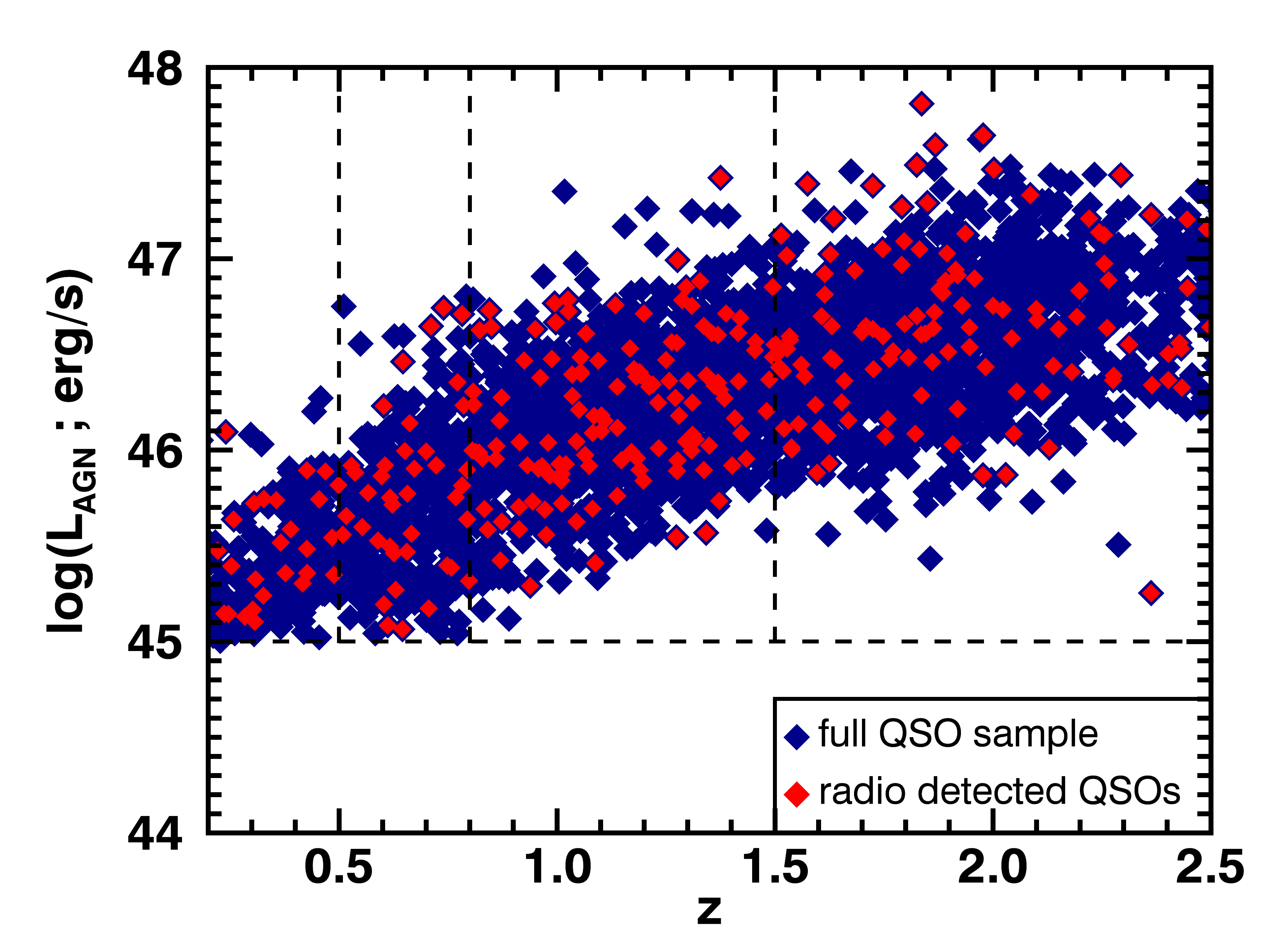
Figure 1: AGN bolometric luminosity ($\mathrel{L_{\rm AGN,bol}}$) versus redshift ($z$) for the full QSO sample from SDSS DR7 covered by H-ATLAS in the NGP, GAMA9, GAMA12, and GAMA15 fields. The vertical dashed lines indicate the redshift ranges taken in our analysis, and the horizontal dashed line shows the $\mathrel{L_{\rm AGN,bol}}$ cut that defines the sample (see section 2.1). In red we highlight the radio detected sources from the FIRST radio catalogue (see section 2.3). Within the redshift range of interest ($z=$0.2–2.5) there are a total of 3026 optically selected QSOs.

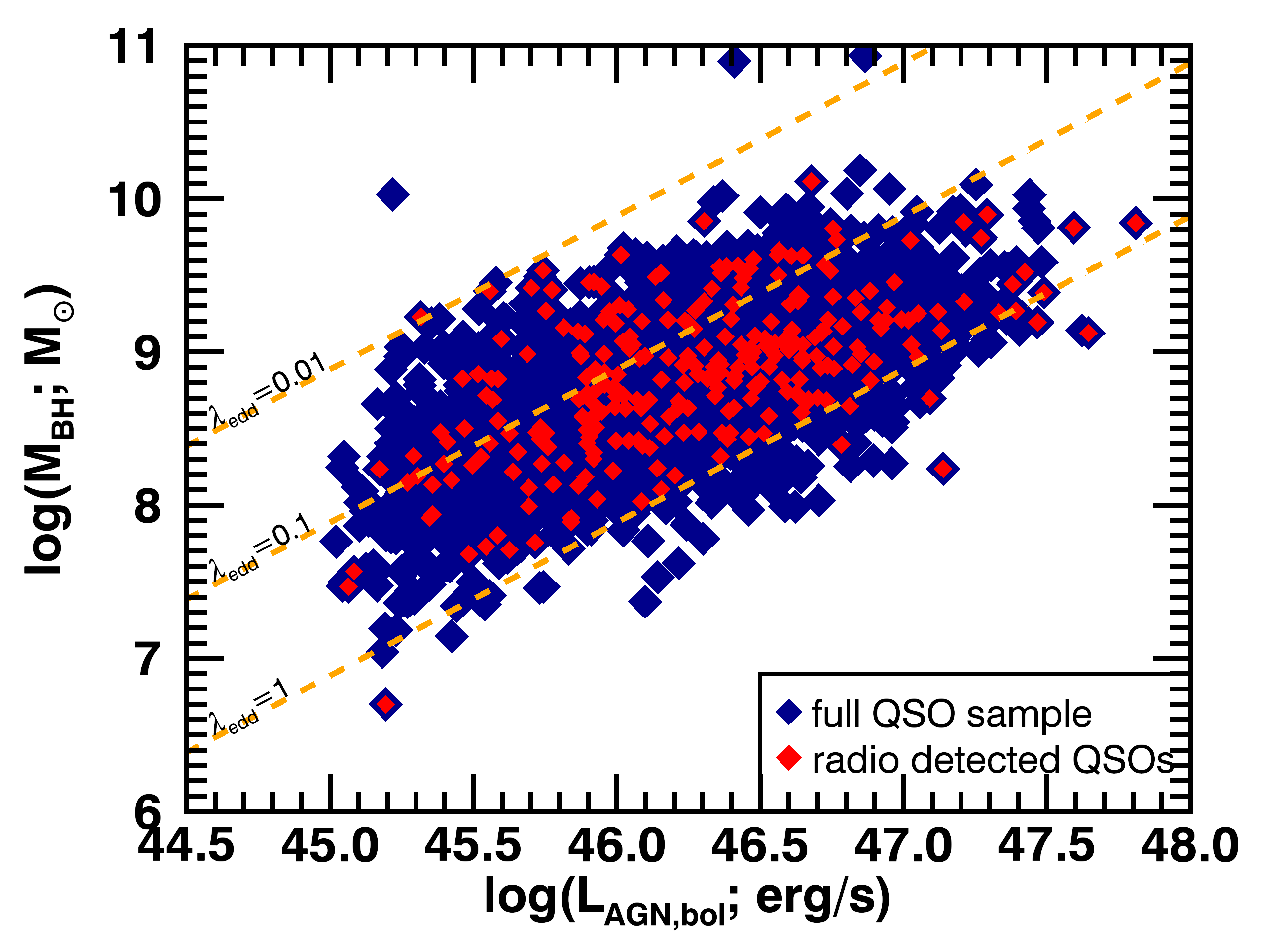
Figure 2: The BH mass ($\mathrel{M_{\rm BH}}$) as a function of AGN bolometric luminosity ($\mathrel{L_{\rm AGN,bol}}$) for the full QSO sample (see section 2). The yellow dashed lines correspond to constant Eddington ratios ($\lambda_{\rm Edd}$ of 0.01, 0.1, and 1), for comparison.

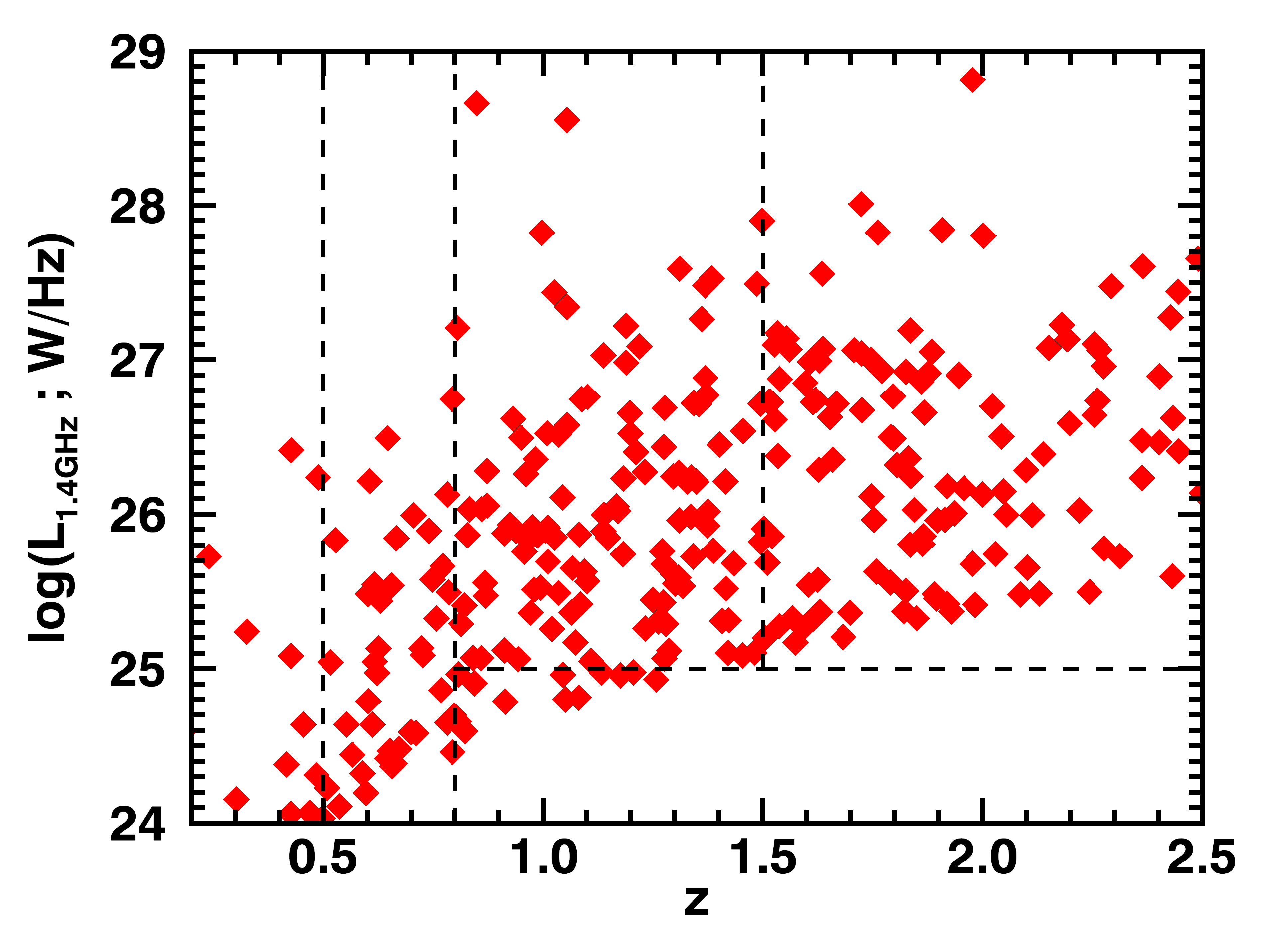
Figure 3: Radio luminosity from the FIRST survey ($\mathrel{L_{\rm 1.4GHz}}$) versus redshift ($z$), for the radio detected QSOs in our sample. The vertical dashed lines indicate the redshift ranges taken in our analysis, and the horizontal dashed lines show the $\mathrel{L_{\rm 1.4GHz}}$ limits used to define sources as radio-luminous. A total of 258 are classified as radio-luminous within the redshift range of interest ($z=$0.2–2.5; see section 2.3).

2.1 Optical/SDSS QSOs

To define our QSO sample we use the publicly available SDSS data release 7 (DR7) QSO catalogue as presented in Shen et al. (2011) (see also Schneider et al. 2010 for original selection of QSOs). We chose this release as it includes the spectral analysis and virial BH mass estimates.

To provide a measurement of the power of the QSOs we use the AGN bolometric luminosity ($\mathrel{L_{\rm AGN,bol}}$) as given in Shen et al. (2011), which has been derived from $L_{\rm 5100\AA}$, $L_{\rm 3000\AA}$, and $L_{\rm 1350\AA}$, for sources at redshifts of $z<$0.7, 0.7$\leq z<$1.9, and $z\geq$1.9 respectively, using the spectral fits and bolometric corrections from the composite SED in Richards et al. (2006) (BC${}_{\rm 5100\AA}=$ 9.26, BC${}_{\rm 3000\AA}=$ 5.15 and BC${}_{\rm 1350\AA}=$ 3.81; see Shen et al. 2011). All the QSOs of our sample have bolometric luminosities of $\mathrel{L_{\rm AGN,bol}}\gtrsim 10^{45}\mathrel{\rm erg\;s^{-1}}$ (see Figure 1). We constrain the sample of QSOs within the regions covered by H-ATLAS.

We also make use of the virial BH mass ($\mathrel{M_{\rm BH}}$) estimates from Shen et al. (2011), from which we estimate the stellar masses (see section 5.2.1 and Eq. 4). The $\mathrel{M_{\rm BH}}$ have been calculated using the FWHM and continuum luminosities of the H$\beta$, Mg II, and C IV lines (see section 3 of Shen et al. 2011). Specifically, the $\mathrel{M_{\rm BH}}$ is estimated from H$\beta$ for sources with redshifts of $z<$0.7, from Mg II for sources with 0.7$<z\leq$1.9, and from C IV for sources with $z>$1.9. In Figure 2 we show the $\mathrel{M_{\rm BH}}$ values of our sample as a function of $\mathrel{L_{\rm AGN,bol}}$. For comparison we also indicate three different levels of the Eddington ratio, $\lambda_{edd}$, the ratio of $\mathrel{L_{\rm AGN,bol}}$ over the Eddington luminosity. The $\lambda_{edd}$ of our sample covers a dynamic range of 3 orders of magnitude, with a mean and median value of 0.34 and 0.24, respectively.

Overall, this study looks at sources with redshifts of $z=$ 0.2–2.5, and includes a total of 3026 QSOs, with BH masses and AGN bolometric luminosities of predominantly $10^{7}<\mathrel{M_{\rm BH}}<10^{10}M_{\odot}$, and $10^{45}<\mathrel{L_{\rm AGN,bol}}<3\times 10^{47}\mathrel{\rm erg\;s^{-1}}$, respectively.

2.2 Mid-infrared and Far-infrared photometry

For our analysis we stack the matched-filter-smoothed PACS and SPIRE image products provided by the H-ATLAS team (see Valiante et al. 2016) for the four fields of GAMA09 (54 deg²), GAMA12 (54 deg²), GAMA15 (54 deg²), and NGP (150 deg²) that overlap with the SDSS survey. Detailed information on the construction of the images is presented in Valiante et al. (2016). The images used in our analysis have had the large scale background subtracted (i.e., the cirrus emission within our galaxy), and each pixel contains the best estimate of the flux density of a point source at that position, making them ideal for stacking analyses. In addition to the images there are also noise maps available that provide the instrumental noise at each pixel.

To define the MIR properties of our sample we use the WISE all-sky survey (Wright et al. 2010). Using a radius of 1$"$ we match to the optical positions of our QSO sample described in section 2.1, with a spurious match fraction of $\sim$0.1%. We find that 94.2% of our sources have a WISE counterpart. Sources in the catalogue with less than a 2$\sigma$ significance at a given band, have been attributed an upper limit defined by the integrated flux density measurement plus two times the measurement uncertainty. In the cases were the flux density is negative then the upper limit is defined as two times the measurement uncertainty (see the explanatory supplement to the WISE All-Sky data release, accessible through the link given in footnote 1). For our SED fitting analysis (section 3.3) we use the W3 and W4 bands at 12$\mathrel{\rm\mu m}$ and 22$\mathrel{\rm\mu m}$, respectively.

2.3 Radio data and classification

To determine the radio luminosities of our QSO sample we use the FIRST radio catalogue (Becker, White & Helfand 1995), which covers the full sky area observed by SDSS, to a sensitivity of 1 mJy. To identify the radio detected QSOs we matched the SDSS QSO catalogue to the FIRST catalogue using a 2$"$ radius, to minimise the number of spurious matches, with a resulting spurious match fraction of $\sim$1.4% (see footnote 2). We calculate the 1.4GHz luminosity ($\rm L_{1.4GHz}$) from the catalogued flux densities, using the following equation:

$$L_{1.4GHz}=4\pi D^{2}F_{1.4GHz}(1+z)^{-(1-\alpha)}$$ (1)

where D is the luminosity distance, $\rm F_{1.4GHz}$ is the catalogued flux density, and assuming $f_{v}\propto v^{-\alpha}$ with a spectral index of $\alpha=$0.8. In Figure 3 we plot the radio luminosity of the radio detected sources as a function of redshift.

We classify sources as radio-luminous AGN, using a luminosity lower limit cut of $L_{\rm 1.4GHz}>$ 10${}^{24}\rm W\,Hz^{-1}$ for $z\,<$ 0.8, and $L_{\rm 1.4GHz}>$ 10${}^{25}\rm W\,Hz^{-1}$ for $z\,>$ 0.8 (see Figure 3). Based on work from McAlpine, Jarvis & Bonfield (2013), Magliocchetti et al. (2016) argue that the radio luminosity beyond which the contribution by star-forming galaxies to the total radio luminosity function becomes negligible, increases from 10${}^{22.8}\rm W\,Hz^{-1}$ in the local Universe up to $\rm L_{1.4GHz,limit}=10^{24.6}\rm W\,Hz^{-1}$ at redshift of $z\sim$ 1.8, after which it remains constant. Our luminosity cut is always higher than these thresholds, indicating that we are selecting sources where the AGN is dominating the radio emission, and do not expect star forming galaxies to be contaminating our selection. Furthermore, in section 4.3 we demonstrate how the radio luminosities of this sample are $>$1–3 orders of magnitude higher than the radio luminosities predicted from the IR luminosities due to star-formation. Therefore we are selecting only AGN dominated radio sources. Within the redshift range studied here ($z=$ 0.2–2.5), there are 258 QSOs classified as radio-luminous.

3 Analysis

For this study we measure the average SFRs of 3026 optical QSOs as a function of their bolometric luminosity and redshift. We use multi-wavelength photometry covering the MIR–FIR wavelengths (12–500$\mathrel{\rm\mu m}$) to perform SED fitting. With the sample of QSOs explored in this study we can extend the SFR – $\mathrel{L_{\rm AGN,bol}}$ plane of Stanley et al. (2015) by an order of magnitude in AGN luminosity, with 3026 sources covering the luminosities of $\mathrel{L_{\rm AGN,bol}}=$ 10⁴⁵–10${}^{48}\mathrel{\rm erg\;s^{-1}}$. Following Stanley et al. (2015), we have divided our sample in four redshift ranges, $z=$ 0.2–0.5, 0.5–0.8, 0.8–1.5, and 1.5–2.5, which then are split in $\mathrel{L_{\rm AGN,bol}}$ bins of roughly equal number of sources (80–100 sources; see Table 1). For each $z$–$\mathrel{L_{\rm AGN,bol}}$ bin we performed stacking analysis in the Herschel PACS and SPIRE bands to estimate the mean 100$\mathrel{\rm\mu m}$, 160$\mathrel{\rm\mu m}$, 250$\mathrel{\rm\mu m}$, 350$\mathrel{\rm\mu m}$, and 500$\mathrel{\rm\mu m}$ fluxes (section 3.1). We also calculate the mean 12$\mathrel{\rm\mu m}$ and 22$\mathrel{\rm\mu m}$ WISE fluxes (section 3.2), and mean bolometric AGN luminosities from the optical data (see section 2.2). We then used the mean fluxes of each $z$–$\mathrel{L_{\rm AGN,bol}}$ bin to perform composite SED fitting to decompose the IR luminosity into the AGN and star formation contributions (section 3.3). The combination of the multi-wavelength stacking and SED fitting, provides constraints on the mean IR luminosity due to star formation free from the possible AGN contamination, and the uncertainties of monochromatic estimations.

3.1 Stacking Herschel photometry

In this section we describe the methods followed to calculate the mean stacked flux density for each $z$–$\mathrel{L_{\rm AGN,bol}}$ bin in our analysis. For each bin we perform a weighted mean stack of the H-ATLAS PACS-100$\mathrel{\rm\mu m}$, 160$\mathrel{\rm\mu m}$, and SPIRE-250$\mathrel{\rm\mu m}$, 350$\mathrel{\rm\mu m}$, and 500$\mathrel{\rm\mu m}$ images at the optical positions of the SDSS QSOs. In all cases we regrid the images to pixels of 1$"$, so as to have more accurate central positioning. We used the noise maps to define the weighting on the mean, by taking the inverse of the noise as the weight, to take into account that instrumental noise changes within the maps. The equation for the weighted mean of each pixel in the stacked image is:

$$\langle x\rangle=\frac{\sum_{0}^{n}x_{i}\times w_{i}}{\sum_{0}^{n}w_{i}}$$ (2)

where $x$ is the flux density of a pixel in the stacked image, $x_{i}$ is the flux density of the equivalent pixel at all images used in the stack, and $w_{i}$ is the inverted flux density at the equivalent pixel of the noise map. We note that the results do not change if we take $w_{i}$ to be the inverse variance, with a difference of $<$2%.

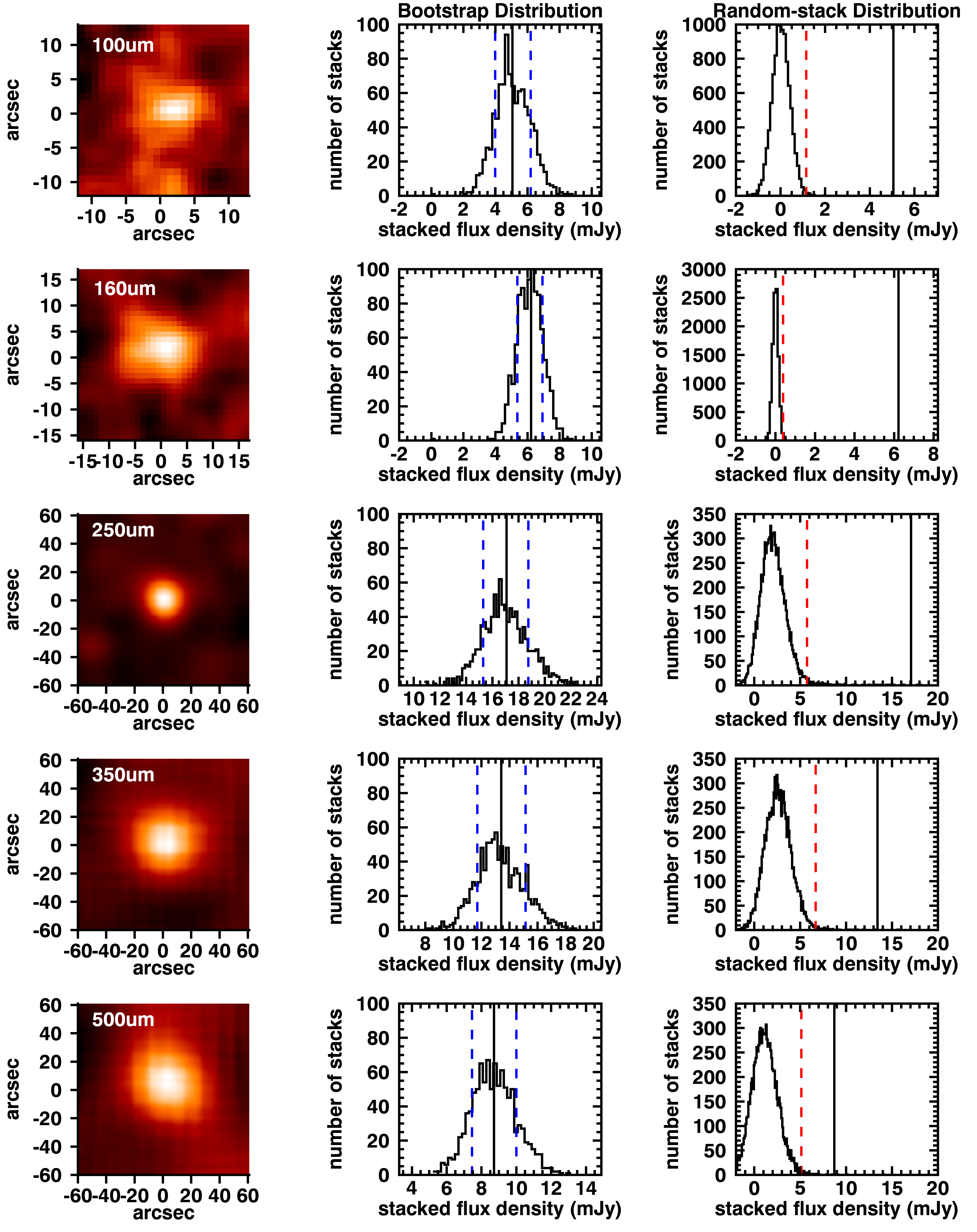
Figure 4: Examples of our stacking procedure for the PACS and SPIRE bands, corresponding to the $z$–$\mathrel{L_{\rm AGN,bol}}$ bin F33 of Table 1. First shown are the stacked images in 100$\mathrel{\rm\mu m}$, 160$\mathrel{\rm\mu m}$, 250$\mathrel{\rm\mu m}$, 350$\mathrel{\rm\mu m}$, and 500$\mathrel{\rm\mu m}$, followed by the bootstrap and random-stack distributions. The bootstrap distribution is a result of randomly re-sampling the sources in the stacks and estimating the stacked mean flux density 1000 times. The mean flux density of the bin is shown with the black line, and in blue dashed lines we show the 16th and 84th percentiles that correspond to the 1$\sigma$ uncertainty on the mean. The random-stack distribution is produced by stacking at random positions in the images, the number of which is defined by the number of sources in the bin. The 99.5th percentile ($\sim 3\sigma$; red dashed line) is the limit we use to define if a stacked flux density is significant (see section 3.1).

From the mean stacked image (see Figure 4) we measure the mean flux density of each $z$–$\mathrel{L_{\rm AGN,bol}}$ bin. For the PACS stacks, which are in units of Jy/pixel, we integrate the flux density within an aperture of 3$"$ radius and use the recommended aperture corrections of 2.63, and 3.57, for 100$\mathrel{\rm\mu m}$ and 160$\mathrel{\rm\mu m}$, respectively (Valiante et al. 2016). For the SPIRE stacks, which are in units of Jy/beam, we take the flux density of the central pixel.

To ensure that a stacked flux density measurement is significant, and above the noise, we perform random stacks within the image. Random stacks are stacks that are calculated for a number of random positions on the map. Because each bin includes a different number of sources from each field, we perform random stacks for each bin individually, and require that the number of random positions to be taken from each field is the same as that used to produce the stack image for the sources in the bin. We perform 10000 random stacks of the maps following the same procedure as for the stack images of the sources, to create a distribution of randomly stacked values. Examples of the resulting random stack distributions for all the bands are shown in Figure 4. The resulting random stack distributions for the SPIRE bands are not centred on zero, but are positively offset by typical values of 1.3 mJy, 2 mJy, and 0.5 mJy, for the 250$\mathrel{\rm\mu m}$, 350$\mathrel{\rm\mu m}$, and 500$\mathrel{\rm\mu m}$, respectively. The offset is caused by the fact that random stacks will include positive flux density from the confused background (i.e., blending of faint sources). These are taken into account for the science stacks below. We fit a Gaussian to each random stack distribution, and from the fit we calculate the $\sigma$ of the distribution. We use the 3$\sigma$ of the random-stack distribution plus the non-zero offset as our detection limit. If the stacked flux density measurement is above the defined limit then it is a detection and we use its absolute value, if it is below the limit we take an upper limit equal to the 3$\sigma$ value of the random stack distribution.

The offset of the random-stack distribution described above reflects a boosting in flux density from the confusion background that causes a boost in flux density of the individual bins. We therefore remove this offset from the stacked flux density in all bands for all z–$\mathrel{L_{\rm AGN,bol}}$ bins. QSOs are well known for their clustering (e.g., White et al. 2012 and references therein), which may cause an additional boost to the stacked flux densities. In Wang et al. (2015) it was found that due to clustering of other dusty star-forming galaxies around optical QSOs there is a $\sim$ 8–13% contamination to the 250$\mathrel{\rm\mu m}$–500$\mathrel{\rm\mu m}$ flux density, respectively. To place an estimate on the possible contamination due to neighbouring sources, we fit the radial light profile of the stacked images using a combination of the PSF model and a constant contamination factor constrained at longer radii (see Appendix B). We find that the contamination derived using our simple method is equivalent, to the offsets found within the random stack distributions of our bins. Consequently, the contamination measured here is still only constraining the confusion background of our stacks. It is possible that there is additional contamination due to clustering that our method is not able to constrain. However, an additional contamination of $\sim$10% in the SPIRE bands will not affect our final results on the IR luminosity by more than their 1$\sigma$ uncertainties.

The uncertainties on the mean fluxes are estimated using the bootstrap technique. We perform 1000 re-samplings for each bin, by randomly selecting 80% of the sources in each bin, and calculate the mean flux density of each. From the resulting distribution of mean flux densities we can define the 1$\sigma$ uncertainties by taking the 16th and 84th percentiles (see examples in Figure 4).

3.2 Mean flux densities of the WISE counterparts

For each $z$–$\mathrel{L_{\rm AGN,bol}}$ bin of our sample we took the mean flux densities at 12$\mathrel{\rm\mu m}$ and 22$\mathrel{\rm\mu m}$ for the sources with a WISE counterpart. The fraction of sources with upper limits in the 12 and 22$\mathrel{\rm\mu m}$ bands ranges between the $z$–$\mathrel{L_{\rm AGN,bol}}$ bins, with a median of 1.3% and 32% respectively. When present the limits show a random enough distribution amongst the measured flux densities to allow us to use the non-parametric Kaplan-Meier estimator for the calculation of the mean of each bin, including both upper limits and measured flux densities (K-M method; e.g., Stanley et al. 2015; see Feigelson & Nelson 1985 for more details). We use this method for the estimation of the mean WISE fluxes in each bin of our sample. We chose this method over stacking the WISE photometry, as the source extraction that has been performed by the WISE team has taken into account of instrumental effects (Wright et al. 2010), providing good quality photometry. To test how the modest fraction of sources with WISE upper limits could affect the uncertainties on our estimations, we take two extreme cases, where all the upper limit sources are given a value of 0, and where all upper limit sources are assumed detections at that limit. We calculate the mean flux density for both approaches in all $z$–$\mathrel{L_{\rm AGN,bol}}$ bins, and find that the range between the two approaches is less than 0.15 mJy in the 12$\mathrel{\rm\mu m}$ band, and less than 2 mJy in the 22$\mathrel{\rm\mu m}$ band, and the mean calculated with the K-M method always lies within the range of these values. Based on this we trust that the K-M method is giving realistic results. We use bootstrap re-sampling to estimate the 1$\sigma$ uncertainties on the means. We note that the bootstrap uncertainties on the mean fluxes are always smaller than the range estimated for the extreme cases above.

3.3 Composite SED fitting

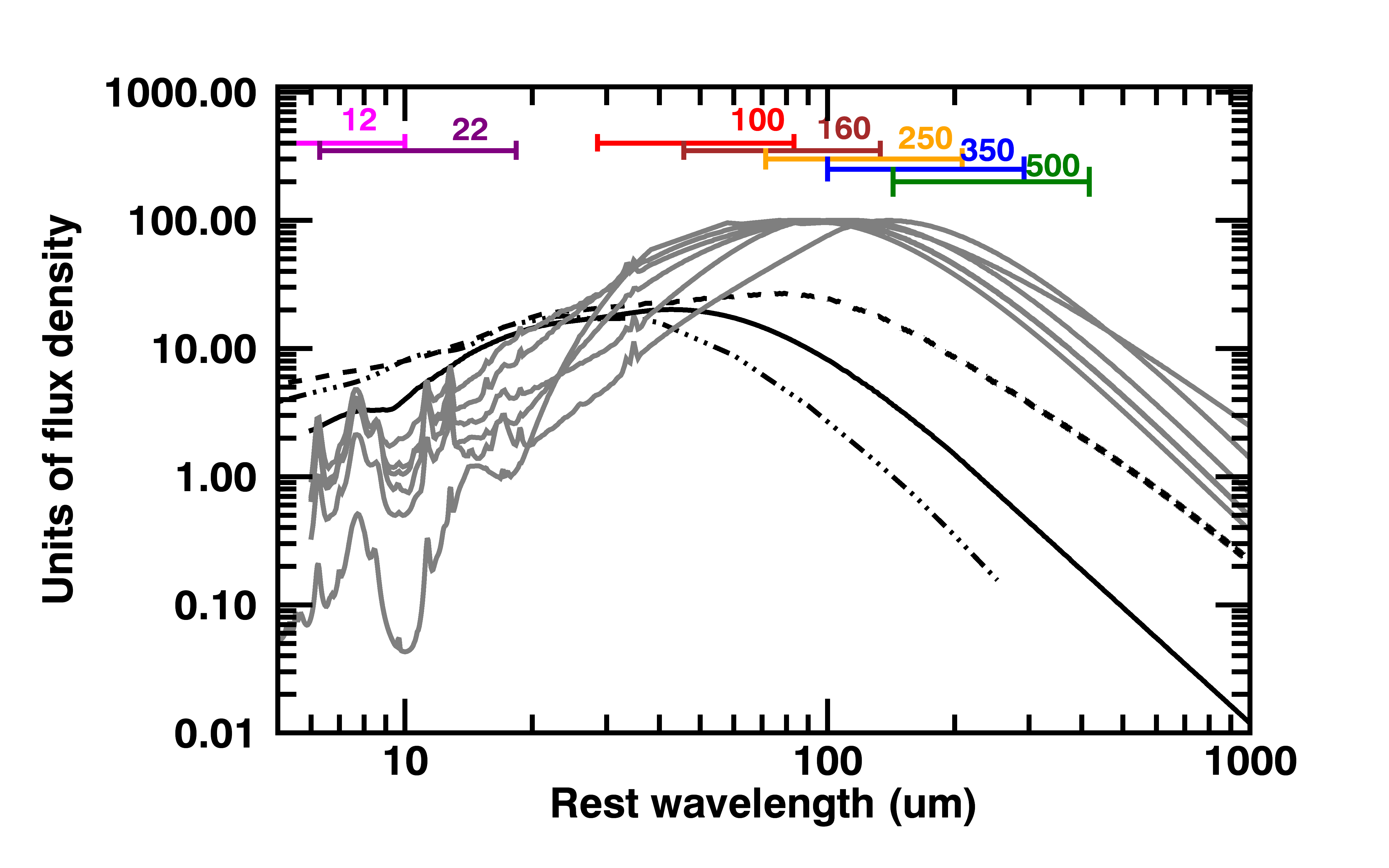
Figure 5: The normalised IR SED templates used in our analysis, for comparison, plotted in arbitrary units of flux density as a function of rest-frame wavelength. With grey curves we show the six SF galaxy templates, that include the five templates derived by Mullaney et al. 2011 and Arp220 by Silva et al. 1998, normalised to the peak flux density. With the black solid curve we show the mean AGN template of Mullaney et al. (2011) template, adopted in our analysis (see section 3.3). Also plotted are two alternative AGN templates, used in section 5.1.2, to test the effect of the choice of AGN template on our results. With the dot-dashed curve we show the AGN template of Mor & Netzer (2012), and with the dashed curve the AGN template of Symeonidis et al. (2016). In coloured horizontal lines we show the wavelength range of the SED covered by the W3 (12$\mathrel{\rm\mu m}$) and W4(22$\mathrel{\rm\mu m}$) WISE bands and the five FIR Herschel bands of 100, 160, 250, 350, and 500$\mathrel{\rm\mu m}$ at redshifts of 0.2–2.5. The 250$\mathrel{\rm\mu m}$ band covers the wavelengths where the star-forming galaxy templates peak for the full redshift range of this study. However, at $z\gtrsim$1 it covers the wavelengths close to the peak of the AGN SED, and hence it could suffer from significant contamination from AGN emission if used as a monochromatic SFR indicator.

In Figure 5 we show how the Herschel bands cover the peak of the star-forming templates at the redshifts of interest, making them essential for the estimation of the SFRs. However, the AGN could also be contributing to the FIR fluxes of each bin, especially at higher redshifts (see Figure 5). For this reason we perform SED fitting to the WISE-12$\mathrel{\rm\mu m}$ and 22$\mathrel{\rm\mu m}$, PACS-100$\mathrel{\rm\mu m}$, 160$\mathrel{\rm\mu m}$, and SPIRE-250$\mathrel{\rm\mu m}$, 350$\mathrel{\rm\mu m}$, and 500$\mathrel{\rm\mu m}$ mean flux densities of each $z$–$\mathrel{L_{\rm AGN,bol}}$ bin, and decompose the AGN and star formation contributions to the IR luminosity.

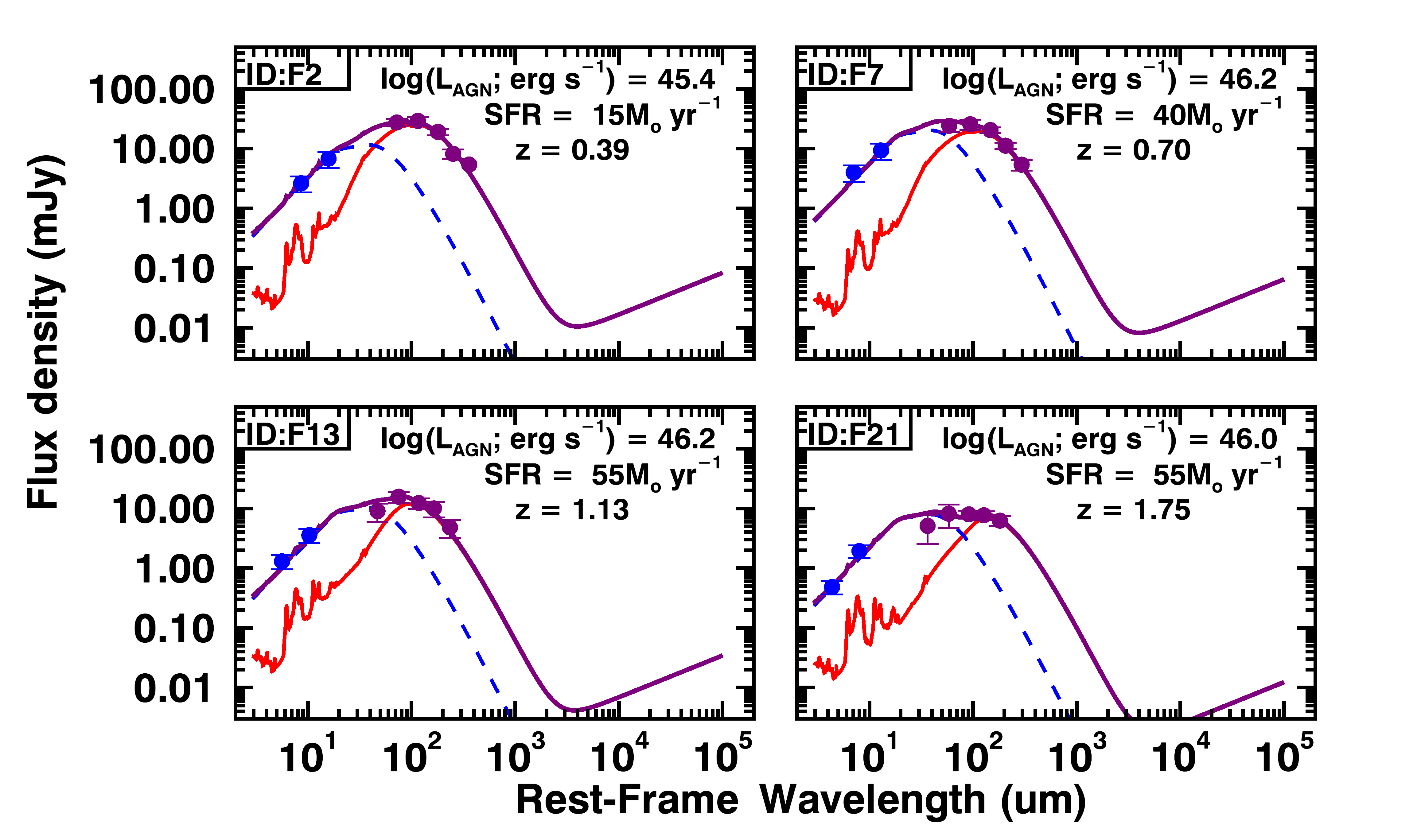
Figure 6: Examples of the SED fits from four $\mathrel{L_{\rm AGN,bol}}$–z bins, one from each of the four redshift ranges (i.e., $z=0.2-0.5,0.5-0.8,0.8-1.5,1.5-2.5$), for the full QSO sample. The blue data points correspond to the mean flux density of WISE bands W3 and W4, while the purple data points correspond to the mean flux density of PACS 100$\mathrel{\rm\mu m}$, 160$\mathrel{\rm\mu m}$, and SPIRE 250$\mathrel{\rm\mu m}$, 350$\mathrel{\rm\mu m}$, and 500$\mathrel{\rm\mu m}$ bands. The blue dashed curve is the best-fitting AGN template, the red solid curve is the best-fitting star-forming template, and the purple solid curve is the resulting overall SED (see section 3.3 for details on the SED fitting analysis). The AGN emission can significantly contribute to the PACS and SPIRE bands, especially at $z\gtrsim 1$.

We follow the methods described in Stanley et al. (2015), which we briefly outline here. We simultaneously fit an AGN template and a set of star-forming templates, and leave the normalisation of the star-forming and AGN template as free parameters in the fit. The set of star-forming templates includes the five originally defined in Mullaney et al. (2011), extended by Del Moro et al. (2013) to cover a wider wavelength range (i.e., 3–10⁵ $\mathrel{\rm\mu m}$; however for the purposes of our SED fitting we are only fitting within the 3–1000$\mathrel{\rm\mu m}$ wavelength region), as well as the Arp220 galaxy template from Silva et al. (1998) (see Figure 5). The AGN template used in our fitting analysis was defined in Mullaney et al. (2011) based on a sample of X-ray AGN, and is shown in Figure 5. For each $z$–$\mathrel{L_{\rm AGN,bol}}$ bin we perform two sets of SED fitting, one using only the six different star-forming templates, and the other using the combination of the AGN and the star-forming templates. Using the BIC parameter (Bayesian Information Criteria; Schwarz 1978) to compare the two sets of fits, we determine if a fit requires the AGN component, and find that all of our bins require the presence of the AGN counterpart in their IR SEDs. The fit with the minimum BIC value is taken to be the best-fitting result. Examples of best-fit SEDs for bins at the four different redshift ranges are given in Figure 6; the resulting best-fit SEDs for all the $z$–$\mathrel{L_{\rm AGN,bol}}$ bins are shown in Appendix A of this paper.

From the resulting best-fit SEDs we calculate the mean IR luminosity due to star formation of each bin, $\mathrel{\langle L_{\rm IR,SF}\rangle}$, by integrating the SF component over 8–1000$\mathrel{\rm\mu m}$. The same is also done to estimate the mean IR (8–1000$\mathrel{\rm\mu m}$) luminosity of the AGN ($\mathrel{\langle L_{\rm IR,AGN}\rangle}$) of each bin. To determine the uncertainty on the $\mathrel{\langle L_{\rm IR,SF}\rangle}$, and $\mathrel{\langle L_{\rm IR,AGN}\rangle}$, we propagate the error on the fit, and the range of luminosities of the fits within $\rm\Delta BIC\,=\,BIC-BIC_{min}\,\leq\,2$ that can be argued to be equally good fits to the best fit (e.g., Liddle 2004). From the calculated $\mathrel{\langle L_{\rm IR,SF}\rangle}$ values we estimate the corresponding mean SFR values by using the Kennicutt (1998) relation corrected for a Chabrier (2003) IMF. For both the SED fitting analyses and the calculation of the IR luminosities, we use the mean redshift of the sources in each $z$–$\mathrel{L_{\rm AGN,bol}}$ bin.

We can see from Figure 6 that as we move towards higher redshifts the strong AGN component, present in all our fits, becomes increasingly dominant in the FIR bands. Indeed, as we show in section 4.1 the AGN can contribute up to 60% to the total IR flux density at redshifts of $z\sim$2. However, as our SED fits show a strong AGN component, the results of this analysis will be dependent on the AGN template of choice.

As an initial test on the suitability of the AGN template of choice, we compare the bolometric AGN luminosity derived from our fitted AGN components to that derived from the optical. To do this we use the 6$\mathrel{\rm\mu m}$ rest-frame luminosity of the fitted AGN components of our bins, and convert to an AGN bolometric luminosity with a bolometric correction factor of 8 (following Richards et al. 2006). We find that the IR derived bolometric AGN luminosity is consistent to the optical-derived bolometric AGN luminosity within a scatter of a factor of $\sim$1.5 around the “1–1” line. Consequently, we trust that the AGN template that we use is reliable for subtracting the AGN contribution to the total IR emission, and therefore for calculating the SFRs of this sample. To further verify our approach, in section 5.1.2 we perform some additional tests using different AGN templates (from Mor & Netzer 2012, and Symeonidis et al. 2016; see dot-dashed and dashed curves in Figure 5) to evaluate the effect the choice of AGN template has on our results. We find that our choice of AGN template is fair and our results will not change significantly for different AGN templates.

To examine if different selection methods could affect the shape of our resulting composite SEDs we have split each $z$–$\mathrel{L_{\rm AGN,bol}}$ bin based on two different selections, and repeat the stacking and SED fitting analysis described in this section. First we have used the WISE colour classification of Stern et al. (2012) for MIR AGN, and find that the majority of sources in the bins (ranging between $\sim$49–-98% for the different bins) are selected as MIR AGN. The resulting composite SEDs of the MIR AGN selected sub-sample, as well as the resulting $\mathrel{\langle L_{\rm IR,SF}\rangle}$ values are consistent to those of the overall sample within a factor of 1.2 for 30/34 of the bins, while the rest lie within a factor of 2–3.3. A second selection was based on wether or not a source is detected at 250$\mathrel{\rm\mu m}$ in the 5$\sigma$ point source catalogue of Valiante et al. (2016), thus selecting FIR luminous sources. Unsurprisingly the majority of our sample is undetected in the FIR, with only 8–19 FIR detected sources in each bin. The resulting composite SEDs of the FIR undetected sub-samples, as well as the resulting $\mathrel{\langle L_{\rm IR,SF}\rangle}$ values, are consistent to those of the overall sample, supporting the idea that the few FIR luminous sources in each bin are not driving the means significantly (something also demonstrated by the bootstrap distributions of our stacks; see Figure 4). Overall, we find that our mean composite SEDs are representative of the full sample and their shape, i.e. the combination of strong AGN and SF components, is still seen when splitting the sample on the MIR or FIR properties, and are not driven by biases caused by MIR or FIR bright sources.

The method followed in this study is significantly different to the one favoured by a number of previous studies performed with H-ATLAS (e.g. Hardcastle et al. 2013; Kalfountzou et al. 2014; Gürkan et al. 2015). In those studies the authors have been using monochromatic 250$\mathrel{\rm\mu m}$ luminosities to derive SFRs, where the other FIR bands are used to derive the temperature of the modified black-body SED using FIR colours. As this method does not take into account the AGN emission at FIR wavelengths, there is a level of uncertainty on the IR luminosity due to star formation, as there is possible AGN contamination; see section 4.1. However, as discussed in sections 4.2 & 4.3 our results are in general agreement with the SFR values reported in previous work, including those mentioned above.

4 Results

Here we present the main results of our study on the mean SFRs of QSOs, following the analysis presented in section 3. Initially, we compare our results of mean SFRs from our composite SEDs, to those from a monochromatic derivation at 250$\mathrel{\rm\mu m}$ (section 4.1). We then investigate the SFR properties of our full QSO sample (section 4.2), and the radio-luminous sub-sample (section 4.3).

4.1 Multi-band SED fitting versus single band derivation for the calculation of star formation luminosities

A common method of previous studies in estimating the SFRs of AGN and QSOs, is using stacking at observed frame 250$\mathrel{\rm\mu m}$ from which the IR luminosity and SFRs are then inferred (e.g., Harrison et al. 2012; Kalfountzou et al. 2014; Gürkan et al. 2015). In this section we compare our results from the multi-wavelength composite SED fitting to the single band 250$\mathrel{\rm\mu m}$ derivation, where we do not take into account the contribution from the AGN. To derive the average IR luminosities (integrated over rest-frame 8–1000$\mathrel{\rm\mu m}$) from the 250$\mathrel{\rm\mu m}$ stacked fluxes, we normalise from the 6 SF galaxy templates that we used in our SED fitting method (see Figure 5, and section 3.3), to the mean flux density at 250$\mathrel{\rm\mu m}$, and take the mean of the resulting IR luminosities of the 6 SF galaxy templates (referred to as $\rm L_{IR,250\mathrel{\rm\mu m}}$).

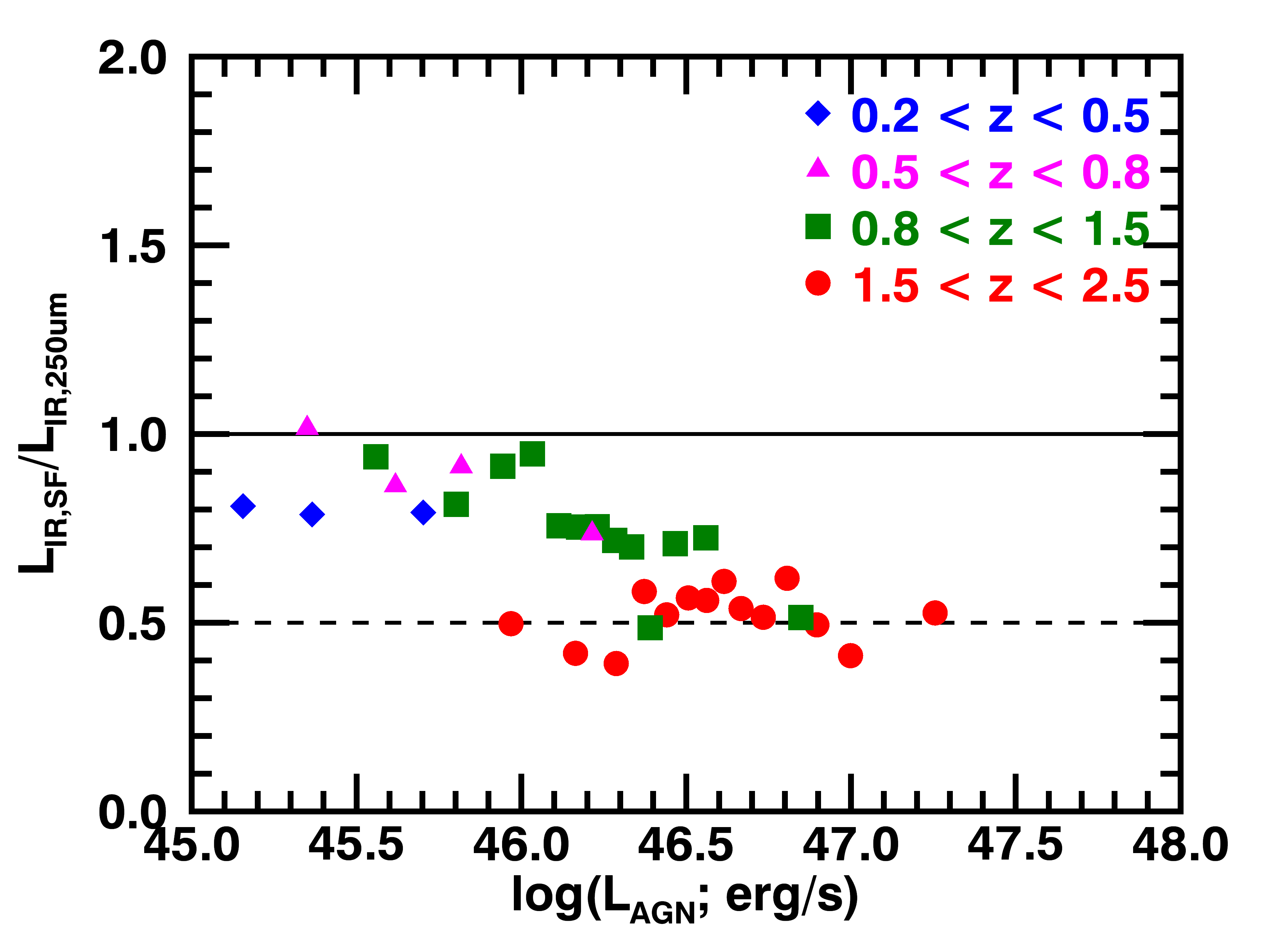
Figure 7: A comparison of the resulting mean IR luminosity due to star formation from our composite SED fitting method ($\mathrel{\langle L_{\rm IR,SF}\rangle}$), compared to the single-band derivation of the IR luminosity from the 250$\mathrel{\rm\mu m}$ band ($\rm L_{IR,250\mathrel{\rm\mu m}}$). The solid line corresponds to the 1–1 line, and the dashed line is a factor of two offset from that. We find that the 250$\mathrel{\rm\mu m}$ band starts to be strongly contaminated by the AGN emission for high luminosity AGN ($\mathrel{L_{\rm AGN,bol}}\gtrsim$10${}^{46}\mathrel{\rm erg\;s^{-1}}$) and at high redshifts ($z\gtrsim$1).

In Figure 7 we compare the results of the two methods described above: (1) the mean IR luminosity derived from the observed frame 250$\mathrel{\rm\mu m}$ photometry and (2) the multi-wavelength SED fitting and decomposition method followed in our analyses. We find that for redshifts of $z\lesssim 0.5$ a single-band derivation from the 250$\mathrel{\rm\mu m}$ band is not affected significantly by the AGN, with a median offset of a factor of 1.2. At redshifts of $z\gtrsim 0.5$ we see a more luminosity-dependent effect, with the $\rm L_{IR,250\mathrel{\rm\mu m}}$ being affected by the AGN by an increasing factor with AGN luminosity, reaching up to a factor of $\approx$2 overestimation at the highest luminosities ($\mathrel{L_{\rm AGN,bol}}>$10${}^{46}\mathrel{\rm erg\;s^{-1}}$). At the highest redshifts of $z\sim 2$ the $L_{\rm IR,250\mathrel{\rm\mu m}}$ is consistently overestimated by a factor of 2–2.5. Similar results on the contribution of the AGN to the total IR luminosity have also been found for higher redshift QSOs ($z\sim 6$; see Schneider et al. 2015).

4.2 The mean SFRs of optical QSOs as a function of the bolometric AGN luminosity

As described in section 3, we split our sample in bins of redshift and $\mathrel{L_{\rm AGN,bol}}$, for which we then estimate the mean $\mathrel{L_{\rm IR,SF}}$ ($\mathrel{\langle L_{\rm IR,SF}\rangle}$) through multi-wavelength stacking and SED fitting that decomposes the AGN and star-forming components.

In Figure 8(a) we present our results on $\mathrel{\langle L_{\rm IR,SF}\rangle}$ as a function of $\mathrel{L_{\rm AGN,bol}}$ and redshift. We see a positive trend of the $\mathrel{\langle L_{\rm IR,SF}\rangle}$ as a function of $\mathrel{L_{\rm AGN,bol}}$ of more than an order of magnitude, something also observed in previous studies (e.g., Bonfield et al. 2011 Rosario et al. 2013; Kalfountzou et al. 2014; Karouzos et al. 2014; Gürkan et al. 2015). However, when splitting in redshift ranges, we find that the observed trend is largely due to the redshift evolution of typical SFR values. Within each redshift range we still see a slight positive trend of $\mathrel{\langle L_{\rm IR,SF}\rangle}$ with $\mathrel{L_{\rm AGN,bol}}$, with the factor of increase ranging from $\sim$1.6–6.3 (0.2–0.8dex), with the highest redshift range of $1.5<z<2.5$ showing the largest increase with $\mathrel{L_{\rm AGN,bol}}$.

In Figure 8(b) we show the $\mathrel{\langle L_{\rm IR,SF}\rangle}$ as a function of the mean BH mass ($\mathrel{\langle M_{\rm BH}\rangle}$) of each bin, and see a positive trend of the $\mathrel{\langle L_{\rm IR,SF}\rangle}$ with $\mathrel{\langle M_{\rm BH}\rangle}$ at all redshifts. This is in agreement with the results of Harris et al. (2016) on QSOs at higher redshifts ($2<z<3$). Since the BH masses and stellar masses of the galaxies correlate (e.g., Kormendy & Ho 2013), an increase in $\mathrel{M_{\rm BH}}$ likely reflects an increase in stellar mass. Consequently, the observed positive trend of the $\mathrel{\langle L_{\rm IR,SF}\rangle}$ with $\mathrel{L_{\rm AGN,bol}}$ (Figure 8(a)) could also be a result of increasing stellar masses (i.e., as seen for the star-forming galaxy population; e.g., Schreiber et al. 2015) rather than AGN luminosity. We explore this further in section 5.2.1.

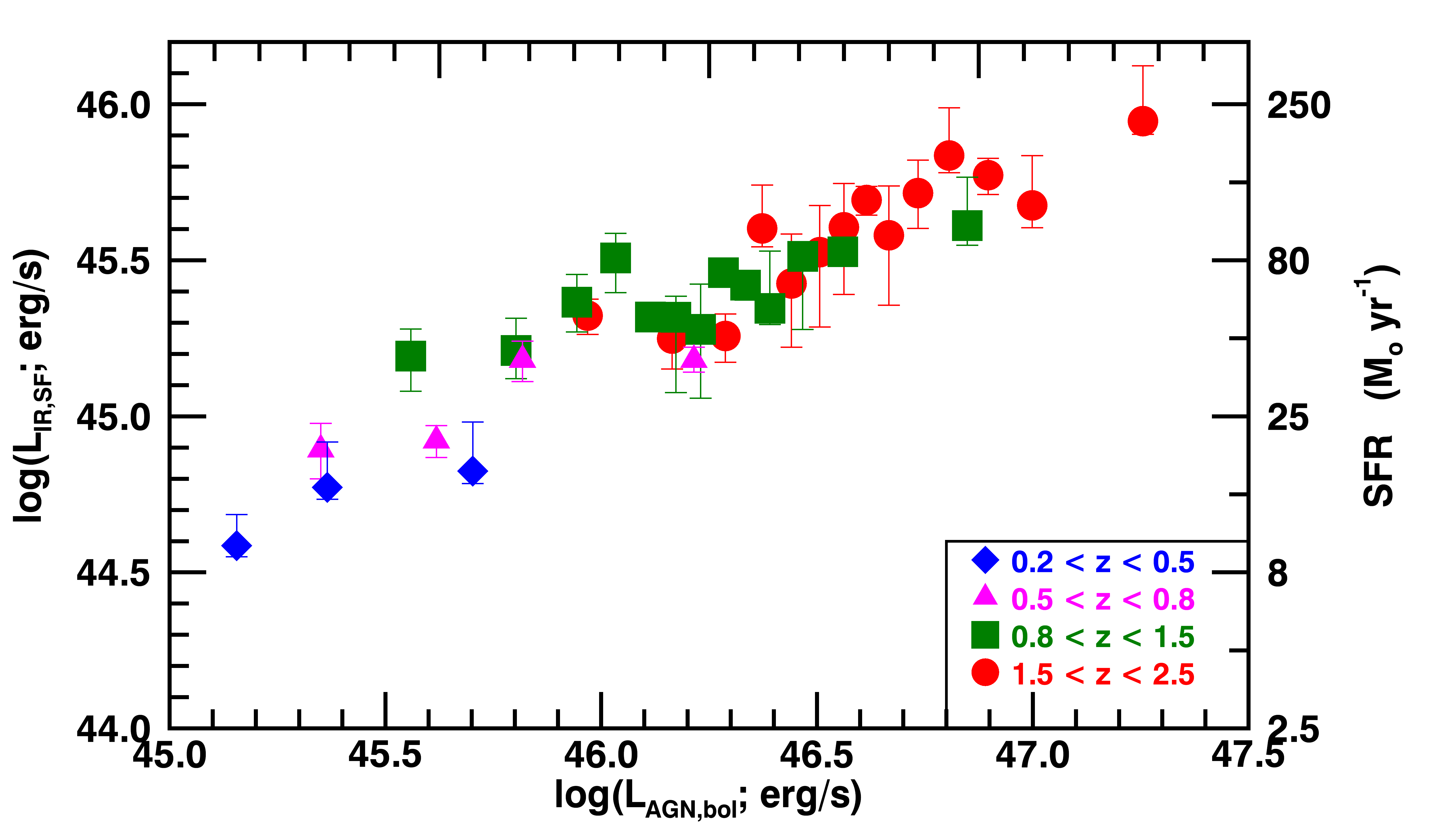
(a)

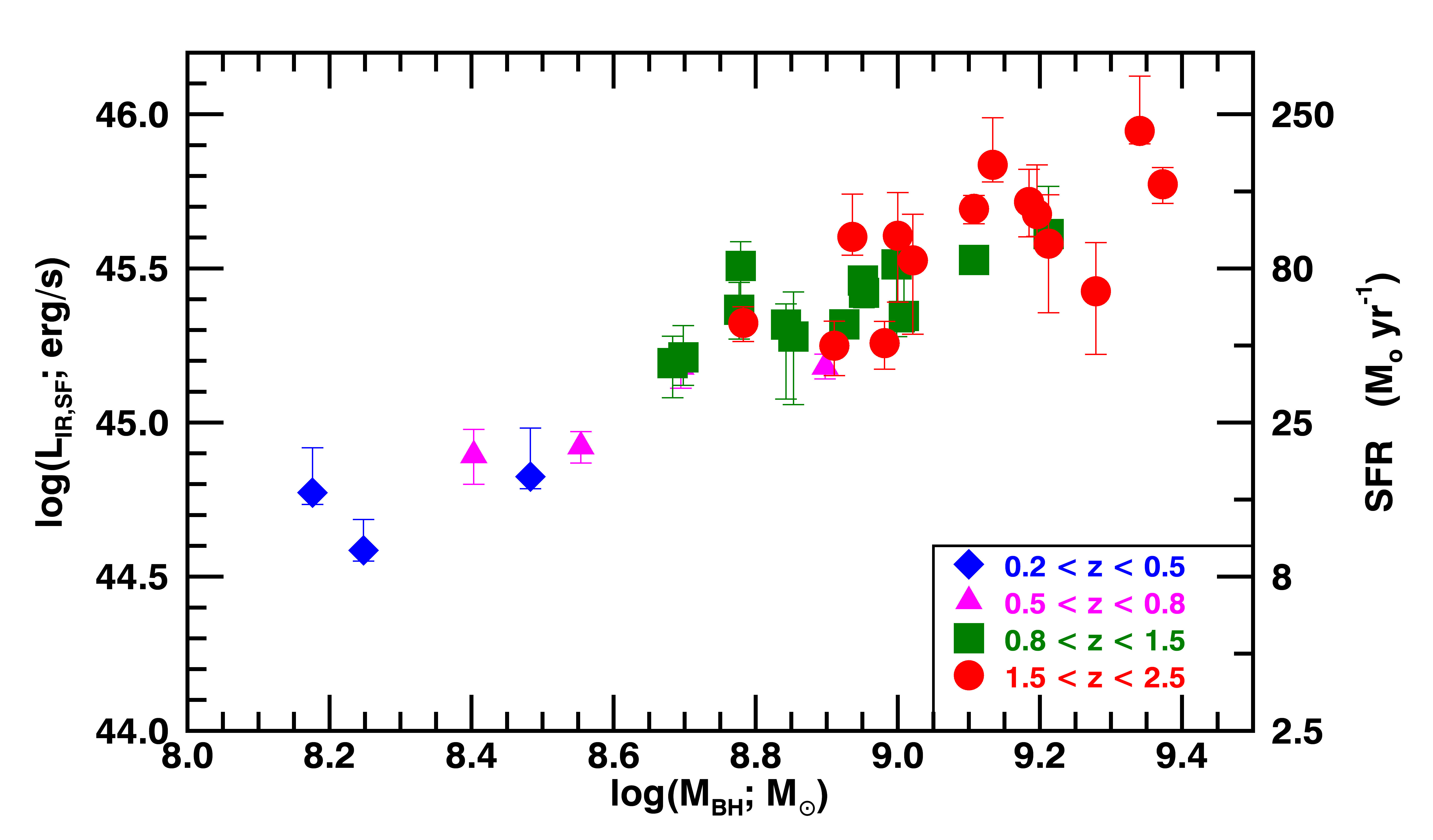
(b)

Figure 8: (a)$\mathrel{\langle L_{\rm IR,SF}\rangle}$ as a function of AGN bolometric luminosity ($\mathrel{L_{\rm AGN,bol}}$). The coloured filled symbols show the results for the full QSO sample in $z$–$\mathrel{L_{\rm AGN,bol}}$ bins. (b)$\mathrel{\langle L_{\rm IR,SF}\rangle}$ as a function of the mean BH mass ($\mathrel{\langle M_{\rm BH}\rangle}$) of each $z$–$\mathrel{L_{\rm AGN,bol}}$ bin. Also provided are the corresponding SFR values estimated using the Kennicutt (1998) relation corrected to a Chabrier IMF (Chabrier 2003). A slight trend of increasing $\mathrel{\langle L_{\rm IR,SF}\rangle}$ with $\mathrel{L_{\rm AGN,bol}}$ is seen for the QSO sample, this positive trend is also seen between the $\mathrel{\langle L_{\rm IR,SF}\rangle}$ and $\mathrel{M_{\rm BH}}$. We argue that the positive trend of $\mathrel{\langle L_{\rm IR,SF}\rangle}$ with $\mathrel{L_{\rm AGN,bol}}$ observed in this sample is mainly driven by mass dependencies (see section 5.2.1).

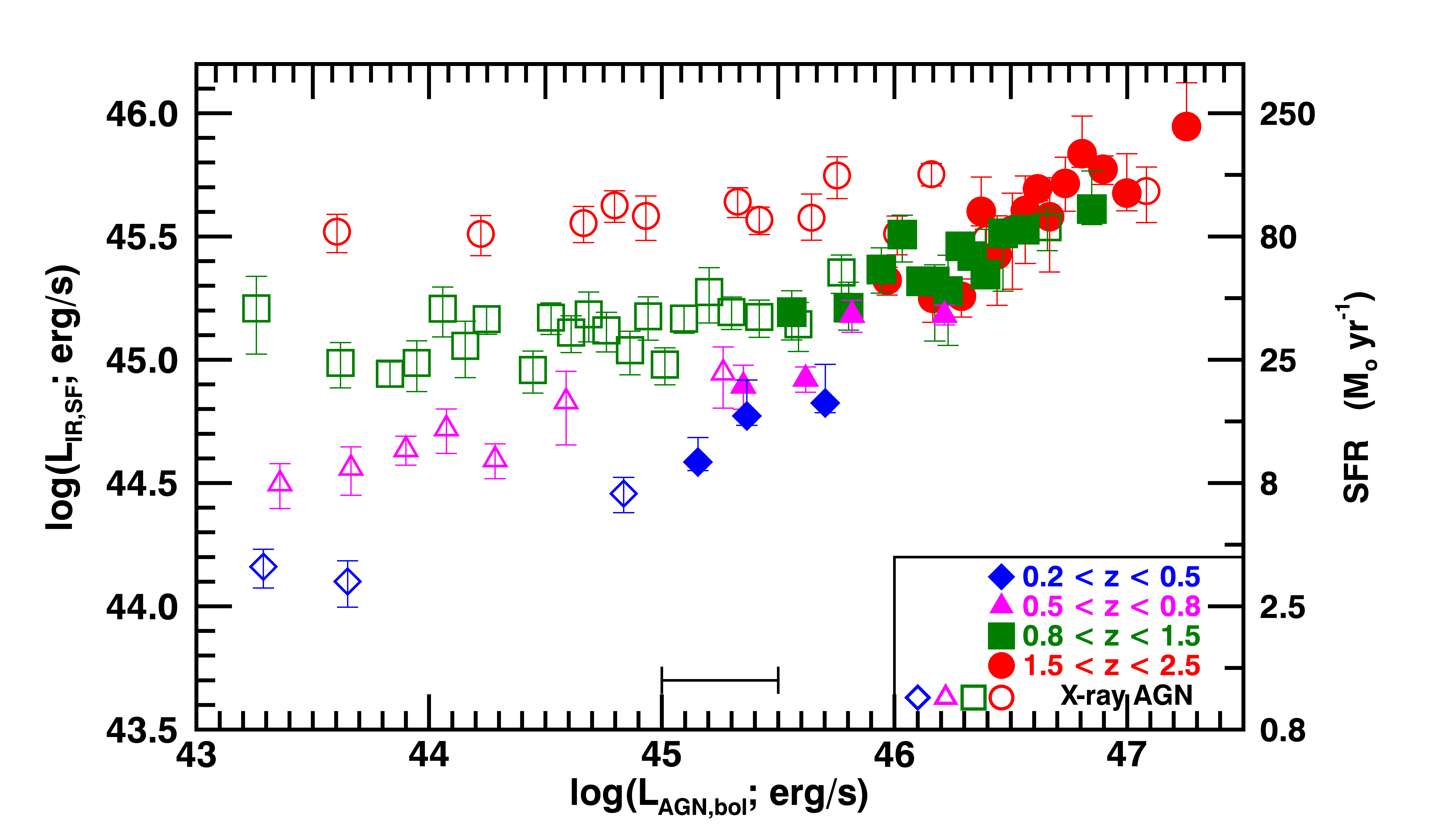
Figure 9: $\mathrel{\langle L_{\rm IR,SF}\rangle}$ as a function of AGN bolometric luminosity ($\mathrel{L_{\rm AGN,bol}}$) for the combination of the X-ray AGN sample from Stanley et al. (2015) and the current sample of optical QSOs. The redshift ranges of the X-ray AGN sample are the same as those of our sample and have been colour–coded to match. Also provided are the corresponding SFR values estimated using the Kennicutt (1998) relation corrected to a Chabrier IMF (Chabrier 2003). The two samples are complementary to each other, and together cover 3–4 orders of magnitude in $\mathrel{L_{\rm AGN,bol}}$. We indicate the 0.5 dex systematic uncertainty between the $\mathrel{L_{\rm AGN,bol}}$ values of the two samples as a range over the x-axis , stemming from the fact that the X-ray AGN sample has $\mathrel{L_{\rm AGN,bol}}$ values derived from X-ray photometry, while for the QSO sample it has been derived from optical photometry (see footnote 3).

ID	$N$	$\langle z\rangle$	$\langle M_{BH}\rangle$	$\langle L_{AGN,bol}\rangle$	$\langle L_{IR,SF}\rangle$
			($\rm M_{\odot}$)	($\rm erg\,s^{-1}$)	($\rm erg\,s^{-1}$)
(a)	(b)	(c)	(d)	(e)	(f)
F 1	83	0.321${}^{+0.078}_{-0.075}$	0.37${}^{+0.25}_{-0.30}\times 10^{9}$	0.14${}^{+0.03}_{-0.02}\times 10^{46}$	0.38${}^{+0.10}_{-0.03}\times 10^{45}$
F 2	80	0.394${}^{+0.067}_{-0.076}$	0.30${}^{+0.21}_{-0.23}\times 10^{9}$	0.23${}^{+0.04}_{-0.03}\times 10^{46}$	0.59${}^{+0.24}_{-0.05}\times 10^{45}$
F 3	88	0.410${}^{+0.059}_{-0.054}$	0.46${}^{+0.09}_{-0.36}\times 10^{9}$	0.50${}^{+0.16}_{-0.18}\times 10^{46}$	0.67${}^{+0.29}_{-0.06}\times 10^{45}$
F 4	94	0.640${}^{+0.114}_{-0.102}$	0.33${}^{+0.24}_{-0.25}\times 10^{9}$	0.22${}^{+0.07}_{-0.07}\times 10^{46}$	0.78${}^{+0.17}_{-0.15}\times 10^{45}$
F 5	89	0.635${}^{+0.107}_{-0.082}$	0.47${}^{+0.25}_{-0.36}\times 10^{9}$	0.42${}^{+0.07}_{-0.07}\times 10^{46}$	0.84${}^{+0.10}_{-0.10}\times 10^{45}$
F 6	94	0.670${}^{+0.098}_{-0.089}$	0.66${}^{+0.48}_{-0.47}\times 10^{9}$	0.66${}^{+0.13}_{-0.09}\times 10^{46}$	1.52${}^{+0.22}_{-0.22}\times 10^{45}$
F 7	96	0.697${}^{+0.076}_{-0.066}$	1.12${}^{+0.60}_{-0.84}\times 10^{9}$	1.64${}^{+0.74}_{-0.73}\times 10^{46}$	1.52${}^{+0.15}_{-0.13}\times 10^{45}$
F 8	85	0.989${}^{+0.161}_{-0.156}$	0.61${}^{+0.40}_{-0.46}\times 10^{9}$	0.36${}^{+0.10}_{-0.11}\times 10^{46}$	1.56${}^{+0.34}_{-0.36}\times 10^{45}$
F 9	86	1.133${}^{+0.210}_{-0.189}$	0.63${}^{+0.54}_{-0.42}\times 10^{9}$	0.63${}^{+0.10}_{-0.10}\times 10^{46}$	2.08${}^{+0.35}_{-0.89}\times 10^{45}$
F10	89	1.100${}^{+0.248}_{-0.236}$	0.80${}^{+0.39}_{-0.55}\times 10^{9}$	0.88${}^{+0.07}_{-0.06}\times 10^{46}$	2.32${}^{+0.52}_{-0.46}\times 10^{45}$
F11	90	1.080${}^{+0.216}_{-0.181}$	0.74${}^{+0.48}_{-0.43}\times 10^{9}$	1.08${}^{+0.08}_{-0.09}\times 10^{46}$	3.22${}^{+0.64}_{-0.73}\times 10^{45}$
F12	86	1.104${}^{+0.255}_{-0.202}$	1.03${}^{+0.44}_{-0.65}\times 10^{9}$	1.30${}^{+0.08}_{-0.06}\times 10^{46}$	2.08${}^{+0.19}_{-0.19}\times 10^{45}$
F13	82	1.132${}^{+0.185}_{-0.166}$	1.01${}^{+0.69}_{-0.64}\times 10^{9}$	1.49${}^{+0.07}_{-0.08}\times 10^{46}$	1.63${}^{+0.44}_{-0.31}\times 10^{45}$
F14	84	1.157${}^{+0.203}_{-0.191}$	0.97${}^{+0.60}_{-0.60}\times 10^{9}$	1.70${}^{+0.07}_{-0.06}\times 10^{46}$	1.90${}^{+0.75}_{-0.76}\times 10^{45}$
F15	82	1.175${}^{+0.181}_{-0.202}$	1.21${}^{+0.90}_{-0.79}\times 10^{9}$	1.92${}^{+0.07}_{-0.07}\times 10^{46}$	2.89${}^{+0.29}_{-0.29}\times 10^{45}$
F16	89	1.223${}^{+0.151}_{-0.140}$	1.14${}^{+0.60}_{-0.65}\times 10^{9}$	2.16${}^{+0.09}_{-0.10}\times 10^{46}$	2.63${}^{+0.28}_{-0.28}\times 10^{45}$
F17	87	1.273${}^{+0.200}_{-0.173}$	1.29${}^{+0.71}_{-0.79}\times 10^{9}$	2.46${}^{+0.10}_{-0.11}\times 10^{46}$	4.08${}^{+1.75}_{-0.55}\times 10^{45}$
F18	85	1.245${}^{+0.202}_{-0.204}$	1.39${}^{+0.67}_{-0.76}\times 10^{9}$	2.93${}^{+0.18}_{-0.19}\times 10^{46}$	3.26${}^{+0.36}_{-1.36}\times 10^{45}$
F19	87	1.254${}^{+0.201}_{-0.187}$	1.74${}^{+0.71}_{-0.87}\times 10^{9}$	3.63${}^{+0.40}_{-0.35}\times 10^{46}$	3.37${}^{+0.31}_{-0.30}\times 10^{45}$
F20	99	1.272${}^{+0.188}_{-0.229}$	2.34${}^{+1.49}_{-1.37}\times 10^{9}$	7.05${}^{+2.42}_{-2.61}\times 10^{46}$	2.22${}^{+1.17}_{-0.25}\times 10^{45}$
F21	86	1.750${}^{+0.158}_{-0.205}$	1.02${}^{+0.74}_{-0.72}\times 10^{9}$	0.93${}^{+0.21}_{-0.23}\times 10^{46}$	2.10${}^{+0.27}_{-0.27}\times 10^{45}$
F22	90	1.847${}^{+0.237}_{-0.236}$	1.22${}^{+0.80}_{-0.86}\times 10^{9}$	1.46${}^{+0.18}_{-0.18}\times 10^{46}$	1.78${}^{+0.36}_{-0.36}\times 10^{45}$
F23	93	1.854${}^{+0.330}_{-0.299}$	1.13${}^{+0.77}_{-0.80}\times 10^{9}$	1.94${}^{+0.18}_{-0.16}\times 10^{46}$	4.94${}^{+0.52}_{-0.52}\times 10^{45}$
F24	88	1.785${}^{+0.330}_{-0.240}$	1.84${}^{+0.98}_{-1.25}\times 10^{9}$	2.36${}^{+0.12}_{-0.11}\times 10^{46}$	4.00${}^{+1.51}_{-0.51}\times 10^{45}$
F25	91	1.777${}^{+0.233}_{-0.217}$	1.69${}^{+1.39}_{-1.12}\times 10^{9}$	2.76${}^{+0.14}_{-0.14}\times 10^{46}$	3.36${}^{+1.38}_{-1.43}\times 10^{45}$
F26	97	1.782${}^{+0.254}_{-0.216}$	1.59${}^{+1.04}_{-1.02}\times 10^{9}$	3.21${}^{+0.18}_{-0.17}\times 10^{46}$	4.04${}^{+1.54}_{-1.58}\times 10^{45}$
F27	90	1.776${}^{+0.209}_{-0.217}$	1.63${}^{+0.98}_{-1.04}\times 10^{9}$	3.65${}^{+0.13}_{-0.13}\times 10^{46}$	2.67${}^{+1.17}_{-1.00}\times 10^{45}$
F28	93	1.853${}^{+0.207}_{-0.251}$	1.97${}^{+1.29}_{-1.34}\times 10^{9}$	4.12${}^{+0.18}_{-0.19}\times 10^{46}$	1.81${}^{+0.32}_{-0.32}\times 10^{45}$
F29	88	1.859${}^{+0.256}_{-0.262}$	2.16${}^{+1.30}_{-1.49}\times 10^{9}$	4.64${}^{+0.26}_{-0.21}\times 10^{46}$	3.80${}^{+1.67}_{-1.53}\times 10^{45}$
F30	80	1.879${}^{+0.224}_{-0.257}$	2.12${}^{+1.33}_{-1.21}\times 10^{9}$	5.42${}^{+0.29}_{-0.29}\times 10^{46}$	5.19${}^{+1.43}_{-1.19}\times 10^{45}$
F31	93	1.911${}^{+0.240}_{-0.244}$	2.30${}^{+0.78}_{-1.22}\times 10^{9}$	6.40${}^{+0.43}_{-0.35}\times 10^{46}$	6.85${}^{+2.89}_{-0.82}\times 10^{45}$
F32	89	2.015${}^{+0.236}_{-0.289}$	2.61${}^{+0.93}_{-1.61}\times 10^{9}$	7.88${}^{+0.70}_{-0.68}\times 10^{46}$	5.93${}^{+0.79}_{-0.79}\times 10^{45}$
F33	94	2.058${}^{+0.299}_{-0.310}$	3.68${}^{+1.93}_{-2.17}\times 10^{9}$	1.00${}^{+0.11}_{-0.08}\times 10^{47}$	4.74${}^{+2.11}_{-0.72}\times 10^{45}$
F34	99	2.053${}^{+0.258}_{-0.246}$	4.76${}^{+2.80}_{-2.79}\times 10^{9}$	1.80${}^{+0.35}_{-0.58}\times 10^{47}$	8.83${}^{+4.46}_{-0.81}\times 10^{45}$

Table 1: Table of the mean source properties for each $z$–$\mathrel{L_{\rm AGN,bol}}$ bin in our sample of optical QSOs. (a) The ID of the bin that corresponds to the SEDs presented in the Appendix. (b) The number of sources in each bin. (c) The mean redshift of each bin. (d) The mean BH mass of each bin. (e) The mean AGN bolometric luminosity (derived from the optical) of each bin. The uncertainties in (c), (d), and (e) correspond to the 16th to the 84th percentiles of the values in each bin. (f) The mean IR luminosity due to star formation from the best-fit SED of each bin, the uncertainties are defined by the combination of the error on the fit and the range of $\mathrel{\langle L_{\rm IR,SF}\rangle}$ values from the other star-forming templates (see section 3.3).

In our previous work (Stanley et al. 2015) we constrained the $\mathrel{\langle L_{\rm IR,SF}\rangle}$ for a sample of X-ray AGN in bins of redshift and $\mathrel{L_{\rm AGN,bol}}$. The sample of X-ray AGN covers 3 orders of magnitude in $\mathrel{L_{\rm AGN,bol}}$ of both moderate and high luminosity AGN ($10^{43}<\mathrel{L_{\rm AGN,bol}}<5\times 10^{47}\mathrel{\rm erg\;s^{-1}}$). The sample of high luminosity optical QSOs in this work is ideal to extend the $\mathrel{\langle L_{\rm IR,SF}\rangle}$–$\mathrel{L_{\rm AGN,bol}}$ plane as defined in Stanley et al. (2015) to the highest $\mathrel{L_{\rm AGN,bol}}$ region. It also allows us to search for systematic differences between the two populations of AGN. In Figure 9 we plot the $\mathrel{\langle L_{\rm IR,SF}\rangle}$ as a function of $\mathrel{L_{\rm AGN,bol}}$ for both the X-ray AGN and optical QSOs extending the $\mathrel{\langle L_{\rm IR,SF}\rangle}$–$\mathrel{L_{\rm AGN,bol}}$ plane to 4 orders of magnitude. Where there is overlap in AGN luminosity between the X-ray selected AGN sample of Stanley et al. (2015) and our current sample of optical QSOs, we see a good agreement in $\mathrel{\langle L_{\rm IR,SF}\rangle}$ values. At the highest redshift range of $1.5<z<2.5$ the $\mathrel{\langle L_{\rm IR,SF}\rangle}$ values of 4 bins at $\log\mathrel{L_{\rm AGN,bol}}<46.4$ of our QSO sample seem in disagreement to those of the X-ray AGN, although they are still consistent within the scatter of the X-ray AGN sample in that redshift range. However, in this comparison the two samples have not been matched in stellar mass, and this may drive some of the differences between the $\mathrel{\langle L_{\rm IR,SF}\rangle}$ values (see section 5.2.1 for a discussion on the effect of mass on the expected $\mathrel{\langle L_{\rm IR,SF}\rangle}$ values). Overall, this comparison shows that the two populations of AGN have consistent mean SFRs at fixed $\mathrel{L_{\rm AGN,bol}}$, and that the $\mathrel{\langle L_{\rm IR,SF}\rangle}$ values as a function of $\mathrel{L_{\rm AGN,bol}}$ of our sample complement and extend the trends observed for the X-ray AGN sample.

4.3 The mean SFRs of Radio-luminous QSOs

In parallel to our analysis of the full sample of QSOs, we also analysed a sub-sample of radio-luminous QSOs selected based on a radio luminosity ($\mathrel{L_{\rm 1.4GHz}}$) cut (see Figure 2 and section 2.3). As we show below, the radio luminosities of our sample are at least an order of magnitude above those corresponding to the $\mathrel{\langle L_{\rm IR,SF}\rangle}$ of our bins, and so we are confident that these radio luminosities are dominated by emission associated with the AGN and not the star formation. For each redshift range we split the sample in $\mathrel{L_{\rm 1.4GHz}}$ bins of roughly equal numbers ($\sim$15–54; see Table 2). Due to the limited number of sources we can only have two bins in each redshift range. For each bin we follow the procedures described in section 3 to estimate $\mathrel{\langle L_{\rm IR,SF}\rangle}$.

In Figure 10 we plot $\mathrel{\langle L_{\rm IR,SF}\rangle}$ as a function of $\mathrel{L_{\rm 1.4GHz}}$ in each bin. We also plot the IR-radio correlation for star-forming galaxies (from Magnelli et al. 2014; Pannella et al. 2015) multiplied by factors of 50, 500, and 5000, to demonstrate how the radio luminosities of our sample are a factor of $\sim$10–5000 above those corresponding to their $\mathrel{\langle L_{\rm IR,SF}\rangle}$ values. In agreement with previous results on radio selected AGN (e.g., Seymour et al. 2011; Karouzos et al. 2014; Kalfountzou et al. 2014; Magliocchetti et al. 2014; Drouart et al. 2014; Gürkan et al. 2015; Drouart et al. 2016; Podigachoski et al. 2016), we find that the radio-luminous QSOs of our sample live in galaxies with significant on-going star formation. Even though we only have two luminosity bins in each redshift range, the $\mathrel{\langle L_{\rm IR,SF}\rangle}$ values as a function of $\mathrel{\langle L_{\rm 1.4GHz}\rangle}$ are suggestive of a flat trend, further implying that the radio luminosity does not originate from the star formation in these systems and also indicating the lack of a direct relationship between the star formation emission of the galaxy and the radio-emission of the QSOs. This is also found in previous studies with different sample selections to ours, such as Seymour et al. (2011), and Drouart et al. (2016).

When comparing the radio-luminous QSOs to the overall QSO sample (dominated by radio-quiet QSOs), the $\mathrel{\langle L_{\rm IR,SF}\rangle}$ values are consistent within scatter, and show similar trends with redshift. This result is also in agreement with previous work by Kalfountzou et al. (2014), comparing radio-loud to radio-quiet QSOs, at similar redshifts and $\mathrel{L_{\rm AGN,bol}}$.

However, in our SED fitting analyses we do not take into account of the synchrotron component that can be present for radio-luminous QSOs. Consequently, our results on the $\mathrel{\langle L_{\rm IR,SF}\rangle}$ could still be contaminated by synchrotron emission due to the AGN. Assuming a conservative spectral index of $\alpha=0.5$, we take the 1.4GHz flux density of the sources in each bin and integrate over 8–1000$\mathrel{\rm\mu m}$ to calculate the total IR luminosity due to synchrotron emission for each source. We compare the mean for each $z$–$\mathrel{L_{\rm 1.4GHz}}$ bin to the corresponding $\mathrel{\langle L_{\rm IR,SF}\rangle}$ values and find that the lower $\mathrel{L_{\rm 1.4GHz}}$ bins of each redshift range are contaminated by $<10$%, but the higher $\mathrel{L_{\rm 1.4GHz}}$ bins of each redshift range can be contaminated by 30–100% making them highly uncertain, with the most uncertain bins having $\mathrel{L_{\rm 1.4GHz}}>10^{27}\rm W/Hz$. More detailed analyses using multi-wavelength radio photometry to constrain the spectral index of the sources, is required to best constrain these results.

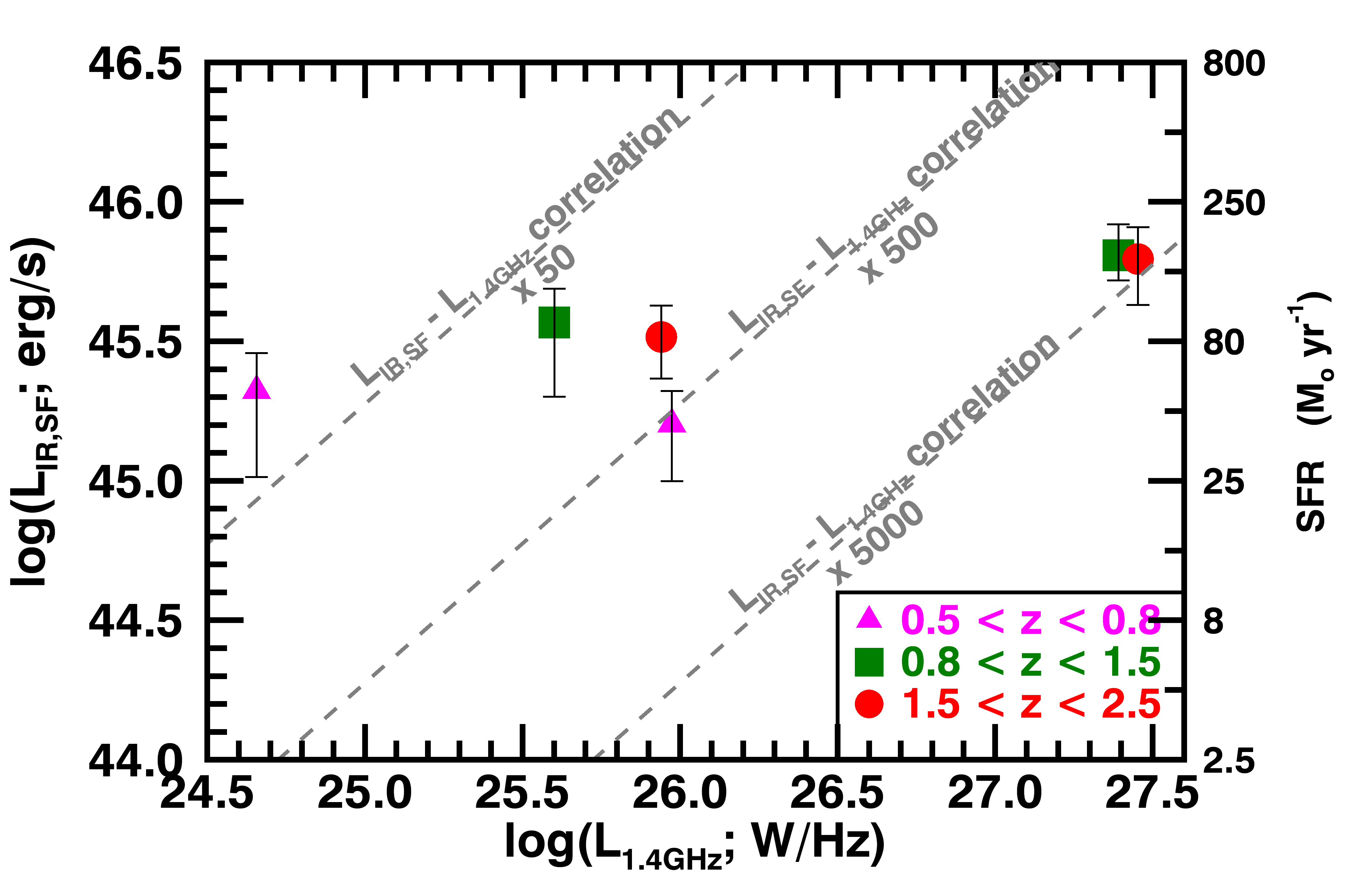
Figure 10: $\mathrel{\langle L_{\rm IR,SF}\rangle}$ in bins of redshift and radio luminosity ($\mathrel{L_{\rm 1.4GHz}}$), as a function of $\mathrel{\langle L_{\rm 1.4GHz}\rangle}$. Also provided are the corresponding SFR values estimated using the Kennicutt (1998) relation corrected to a Chabrier IMF (Chabrier 2003). With dashed lines we indicate the IR-radio relation of star-forming galaxies from Magnelli et al. (2014) increased by factors of 50–5000, to demonstrate that the radio luminosities of our sources cannot be attributed to their star formation. There is no strong evidence for a positive or negative relation between $\mathrel{\langle L_{\rm IR,SF}\rangle}$ and $\mathrel{L_{\rm 1.4GHz}}$, with the general trend being flat. However, for the higher $\mathrel{L_{\rm 1.4GHz}}$ bins of each redshift range the $\mathrel{\langle L_{\rm IR,SF}\rangle}$ could be highly contaminated by synchrotron emission, and therefore these results are uncertain.

ID	$N$	$\langle z\rangle$	$\langle M_{BH}\rangle$	$\langle L_{1.4GHz}\rangle$	$\langle L_{AGN,bol}\rangle$	$\langle L_{IR,SF}\rangle$
			($\rm M_{\odot}$)	($\rm W\,Hz^{-1}$)	($\rm erg\,s^{-1}$)	($\rm erg\,s^{-1}$)
(a)	(b)	(c)	(d)	(e)	(f)	(g)
R1	17	0.663${}^{+0.131}_{-0.074}$	1.27${}^{+2.40}_{-1.07}\times 10^{9}$	0.45${}^{+0.48}_{-0.22}\times 10^{25}$	1.00${}^{+3.44}_{-0.84}\times 10^{46}$	2.60${}^{+0.55}_{-1.30}\times 10^{45}$
R2	15	0.710${}^{+0.076}_{-0.080}$	1.52${}^{+2.99}_{-1.25}\times 10^{9}$	0.94${}^{+2.16}_{-0.81}\times 10^{26}$	1.22${}^{+1.67}_{-0.98}\times 10^{46}$	1.00${}^{+0.17}_{-0.17}\times 10^{45}$
R3	53	1.131${}^{+0.243}_{-0.187}$	1.91${}^{+2.10}_{-1.56}\times 10^{9}$	0.40${}^{+0.33}_{-0.22}\times 10^{26}$	1.99${}^{+1.68}_{-1.45}\times 10^{46}$	4.07${}^{+0.96}_{-2.18}\times 10^{45}$
R4	50	1.180${}^{+0.192}_{-0.218}$	1.52${}^{+0.97}_{-1.20}\times 10^{9}$	2.46${}^{+0.27}_{-2.35}\times 10^{27}$	3.05${}^{+1.60}_{-2.27}\times 10^{46}$	5.17${}^{+1.07}_{-0.89}\times 10^{45}$
R5	54	1.913${}^{+0.308}_{-0.286}$	2.28${}^{+1.12}_{-1.69}\times 10^{9}$	0.87${}^{+1.05}_{-0.64}\times 10^{26}$	5.77${}^{+4.89}_{-4.31}\times 10^{46}$	3.12${}^{+1.48}_{-1.36}\times 10^{45}$
R6	49	1.882${}^{+0.394}_{-0.321}$	2.68${}^{+2.65}_{-1.98}\times 10^{9}$	2.84${}^{+0.76}_{-2.39}\times 10^{27}$	7.92${}^{+8.13}_{-5.99}\times 10^{46}$	4.17${}^{+0.87}_{-0.61}\times 10^{45}$

Table 2: Table of the mean source properties for each $z$–$\mathrel{L_{\rm 1.4GHz}}$ bin in our sub-sample of radio-luminous QSOs. (a) The ID of the bin that corresponds to the set of SEDs presented in the Appendix. (b) The number of sources in each bin. (c) The mean redshift of each bin. (d) The mean BH mass of each bin. (e) The mean radio luminosity at 1.4GHz. (f) The mean AGN bolometric luminosity (derived from the optical) of each bin. The uncertainties in (c), (d), (e), and (f) correspond to the 16th to the 84th percentiles of the values in each bin. (g) The mean IR luminosity due to star formation from the best-fit SED of each bin, the uncertainties are defined by the combination of the error on the fit and the range of $\mathrel{\langle L_{\rm IR,SF}\rangle}$ values from other templates that had good SED fits (see section 3.3).

5 Discussion

In this section we explore the caveats in our method and the possible implications on our results (section 5.1). Following this, we discuss the possible drivers of the weak positive trends of the mean SFR with AGN luminosity seen in our results (section 5.2).

5.1 Verification of our methods

5.1.1 SED broadening

In our SED fitting approach we assume that the observed-frame wavelengths correspond to the rest-frame wavelength of the mean redshift of a given $z$–$\mathrel{L_{\rm AGN,bol}}$ bin, for all of the sources within the bin. That is, we do not take into account modest k-corrections due to the different redshifts of the sources within the stack. This may result in some broadening of the average SED that we did not take into account. However, as our $z$–$\mathrel{L_{\rm AGN,bol}}$ bins have fairly narrow redshift ranges (see Tables 1 & 2) and there is a fairly even scatter around the mean redshift of the bins, we expect that overall there should not be significant broadening effects. To test this, we shift each of our AGN and star-forming templates to the redshift of each source in our $z$–$\mathrel{L_{\rm AGN,bol}}$ bins. For each $z$–$\mathrel{L_{\rm AGN,bol}}$ bin we then take the mean of all the redshifted SED templates to get a mean SED shape, and compare to the original SED template shifted at the mean redshift of the $z$–$\mathrel{L_{\rm AGN,bol}}$ bin. We find that the shape of the mean redshifted SED templates is the same to the original template when shifted to the mean redshift, apart from some smoothing of the SF template PAH features. Consequently, our results on $\mathrel{\langle L_{\rm IR,SF}\rangle}$ are not affected by SED broadening effects.

5.1.2 The choice of AGN template

Since the resulting composite SEDs of our sample show such a strong AGN component, our results may be sensitive to the AGN template that we assume. For this reason, we repeat our analysis using two different AGN templates, that of Mor & Netzer (2012) and that of Symeonidis et al. (2016). The template of Mor & Netzer (2012), derived from a QSO sample with similar methods to Mullaney et al. (2011), has a steeper drop-off at longer wavelengths compared to our default template (see dot-dashed curve in Figure 5). The Symeonidis et al. (2016) template, also derived from a QSO sample, has a more gradual drop-off at longer wavelengths compared to our default template (see dashed curve in Figure 5). The varying contribution of the AGN template at longer wavelengths may affect the $\mathrel{\langle L_{\rm IR,SF}\rangle}$ values estimated by our SED fitting approach.

In the first case, fitting with the Mor & Netzer (2012) AGN template we find that over all $z$–$\mathrel{L_{\rm AGN,bol}}$ bins the results on the $\mathrel{\langle L_{\rm IR,SF}\rangle}$ do not change significantly, with a maximum increase in $\mathrel{\langle L_{\rm IR,SF}\rangle}$ of a factor of $\approx 1.2$, and all bins remaining consistent within the 1$\sigma$ to the original $\mathrel{\langle L_{\rm IR,SF}\rangle}$ results. In the second case where we fit using the Symeonidis et al. (2016) AGN template, we find that up to redshifts of 1.5, the results from using the two templates are consistent within our estimated 1$\sigma$ errors. However, at the highest 1.5–2.5 redshift range, the results using the Symeonidis et al. (2016) template show a much larger scatter to that of our original results, and show no sign of the correlation observed in our original results. Overall, the $\mathrel{\langle L_{\rm IR,SF}\rangle}$ values resulting from fitting with the Symeonidis et al. (2016) template are within a factor of 3 for 31/34 of the $z$–$\mathrel{L_{\rm AGN,bol}}$, with the remaining 3/34 bins, that are in the highest redshift range showing a difference of a factor of $\sim$8. This result highlights that our results for the highest redshift range are the most sensitive to the choice of AGN template used in the SED fitting analysis. However, in the very recent studies of Lani, Netzer & Lutz (2017) and Lyu & Rieke (2017), that looked at the IR AGN SED of PG quasars following a similar approach to that of Symeonidis et al. (2016), it was found that the IR AGN SED has a steeper drop-off at long wavelengths than that argued for in Symeonidis et al. (2016). Indeed, the shape is more similar to that of the Mullaney et al. (2011) and Mor & Netzer (2012) AGN templates. Consequently, even though our highest redshift range is the most sensitive in the AGN template of choice, it is not likely that our results are as strongly affected as the use of a Symeonidis et al. (2016) type template would suggest.

5.2 Understanding the observed trends between the mean SFR and AGN properties.

5.2.1 Comparing to the main sequence of star-forming galaxies

The main sequence of star-forming galaxies is defined from the observed correlation between SFR and stellar mass, and has been found to evolve with redshift (e.g., Noeske et al. 2007; Elbaz et al. 2011; Schreiber et al. 2015). Consequently, the SFR of a normal star-forming galaxy will be dependent on its stellar mass and redshift. In this subsection we test the simple hypothesis that on average QSOs lie on the main sequence of star-forming galaxies. This follows from Stanley et al. (2015), where we showed that when taking into account of the stellar masses and redshifts of the X-ray AGN sample, their mean SFRs are consistent with the main sequence of star-forming galaxies. By comparing our results to the mean SFRs of main sequence galaxies with the same redshift and stellar masses, we can test if the QSO sample shows systematic differences to the overall star-forming population. Furthermore, we can determine if the trends we observe are simply driven by the galaxy properties.

For each $z$–$\mathrel{L_{\rm AGN,bol}}$ bin of our sample we use the BH masses and redshifts of the individual sources to estimate the IR luminosity of main sequence galaxies ($\mathrel{\langle L_{\rm IR,MS}\rangle}$) corresponding to the properties of each. We use Eq. 9 of Schreiber et al. (2015) to calculate the $\mathrel{L_{\rm IR,MS}}$:

$$\begin{split}\log_{10}(SFR_{MS}[M_{\odot}/yr])=m-0.5+1.5r\\ -0.3[max(0,m-0.36-2.5r)]^{2}\end{split}$$ (3)

where $r=\log_{10}(1+z)$, $m=\log_{10}(M_{\star}/10^{9}M_{\odot})$, and $\rm\mathrel{L_{\rm IR,MS}}=SFR_{MS}/4.5\times 10^{-44}$ (we note that Schreiber et al. 2015 assume a Salpeter IMF for Eq. 3 which we take into account here). The 1$\sigma$ scatter in the relation is +/- 0.3dex and remains out to at least a redshift of $\sim$4 (Schreiber et al. 2015). As can be seen in the above equation, to estimate the $\mathrel{\langle L_{\rm IR,MS}\rangle}$ we need a measurement of the stellar masses of our sample. As our sample consists of QSOs, where the QSO emission overpowers that of the host galaxy in the optical, it is very unreliable to use SED fitting methods to the optical photometry to calculate stellar masses. However, BH masses are available for all of the QSOs in our sample from Shen et al. (2011) (see section 2.1), and can be used to infer stellar masses. To convert the BH masses to stellar masses we make use of the equation defined in Bennert et al. (2011), which includes an empirically derived redshift evolution term for redshifts of $z\lesssim 2$.

$$\begin{split}\log_{10}\frac{M_{BH}}{10^{8}M_{\odot}}=1.12\log_{10}\left(\frac{M_{*}}{10^{10}M_{\odot}}\right)+\\ (1.15\pm 0.15)\log_{10}(1+z)-0.68+(0.16\pm 0.06)\end{split}$$ (4)

To establish if our optical QSOs are consistent with being a randomly selected sample from the main sequence of star-forming galaxies, we follow a similar approach to Rosario et al. (2013). For each $z$–$\mathrel{L_{\rm AGN,bol}}$ bin, we perform a Monte-Carlo (MC) calculation of the $\mathrel{\langle L_{\rm IR,MS}\rangle}$ corresponding to the redshifts and masses of the sources in the bin. Using Eq. 4, we define a distribution of possible stellar masses for each QSO based on their BH mass, and pick a random value from the distribution. The width of the stellar mass distribution includes both the scatter in Eq. 4 and the error on the BH mass (provided by Shen et al. 2011; see section 2.1). Based on the chosen stellar mass, and the known redshift of the source we define a log-normal distribution of $\mathrel{L_{\rm IR,MS}}$ values centred at the luminosity from Eq. 3, with a $\sigma$ of 0.3dex (Schreiber et al. 2015). We pick a random value from the distribution of $\mathrel{L_{\rm IR,MS}}$ values for the source. We repeat this approach for all sources in a $z$–$\mathrel{L_{\rm AGN,bol}}$ bin and then calculate the $\mathrel{\langle L_{\rm IR,MS}\rangle}$ of the bin. The above process is repeated 10,000 times for each bin, and results in a distribution of $\mathrel{\langle L_{\rm IR,MS}\rangle}$ from which we can define the mean and 1$\sigma$ range of the possible $\mathrel{\langle L_{\rm IR,MS}\rangle}$ values for a given z–$\mathrel{L_{\rm AGN,bol}}$ bin.

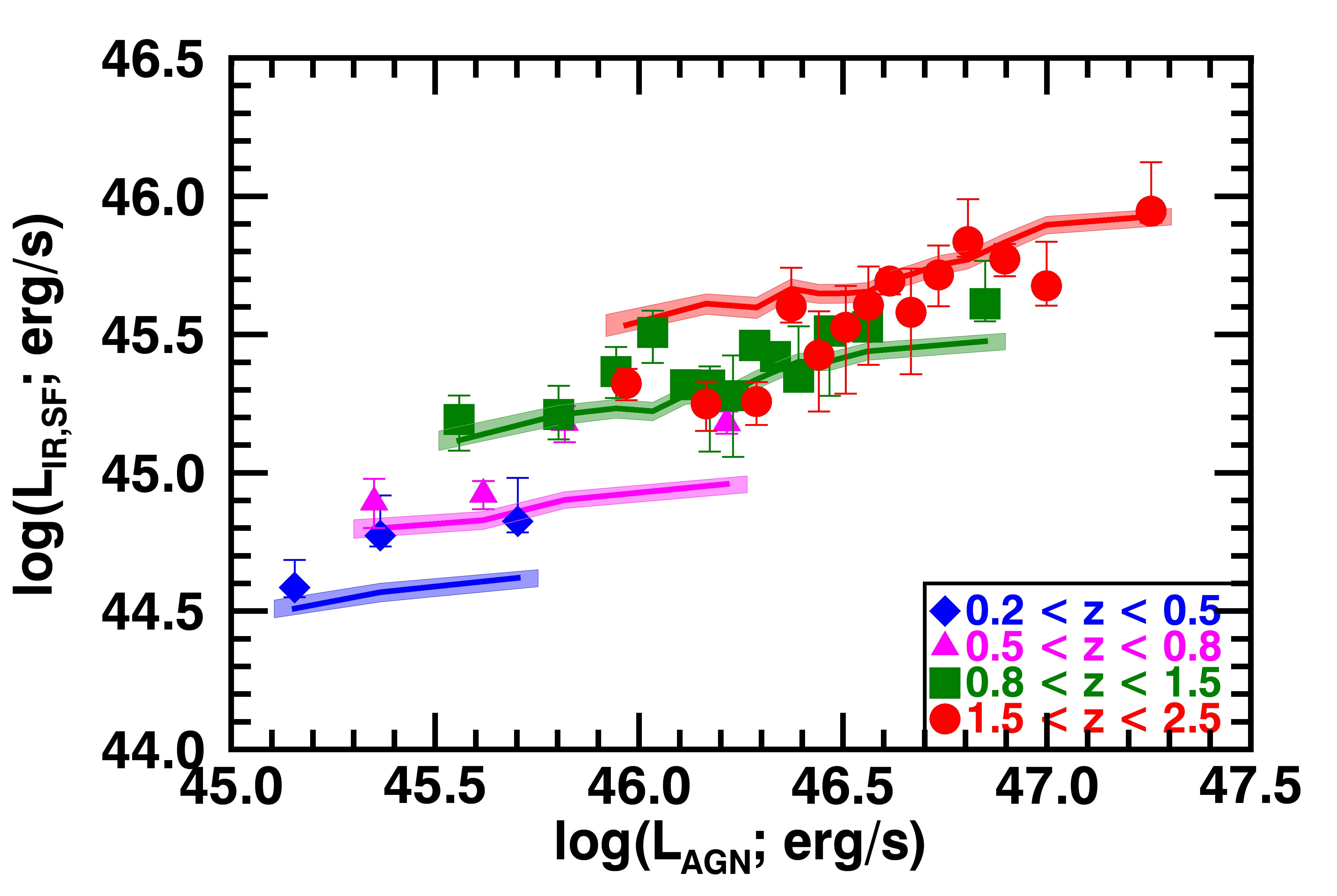
Figure 11: $\mathrel{\langle L_{\rm IR,SF}\rangle}$ as a function of $\mathrel{L_{\rm AGN,bol}}$ for the full QSO sample. The coloured regions indicate the expected range in $\mathrel{\langle L_{\rm IR,MS}\rangle}$ covered by the main sequence galaxies at the stellar mass (as estimated from the $\mathrel{M_{\rm BH}}$) at each of the redshift ranges; the range reflects the bootstrap error on the $\mathrel{\langle L_{\rm IR,MS}\rangle}$ (see section 5.2.1 for details on defining $\mathrel{\langle L_{\rm IR,MS}\rangle}$ and the error calculation). The observed trends between $\mathrel{\langle L_{\rm IR,SF}\rangle}$ and $\mathrel{L_{\rm AGN,bol}}$ are comparable to those of the $\mathrel{\langle L_{\rm IR,MS}\rangle}$, which is dependent on redshift and stellar mass (here inferred from the BH mass). Consequently, we argue that redshift and BH mass dependencies being the primary drivers of the observed trends of $\mathrel{\langle L_{\rm IR,SF}\rangle}$ with $\mathrel{L_{\rm AGN,bol}}$.

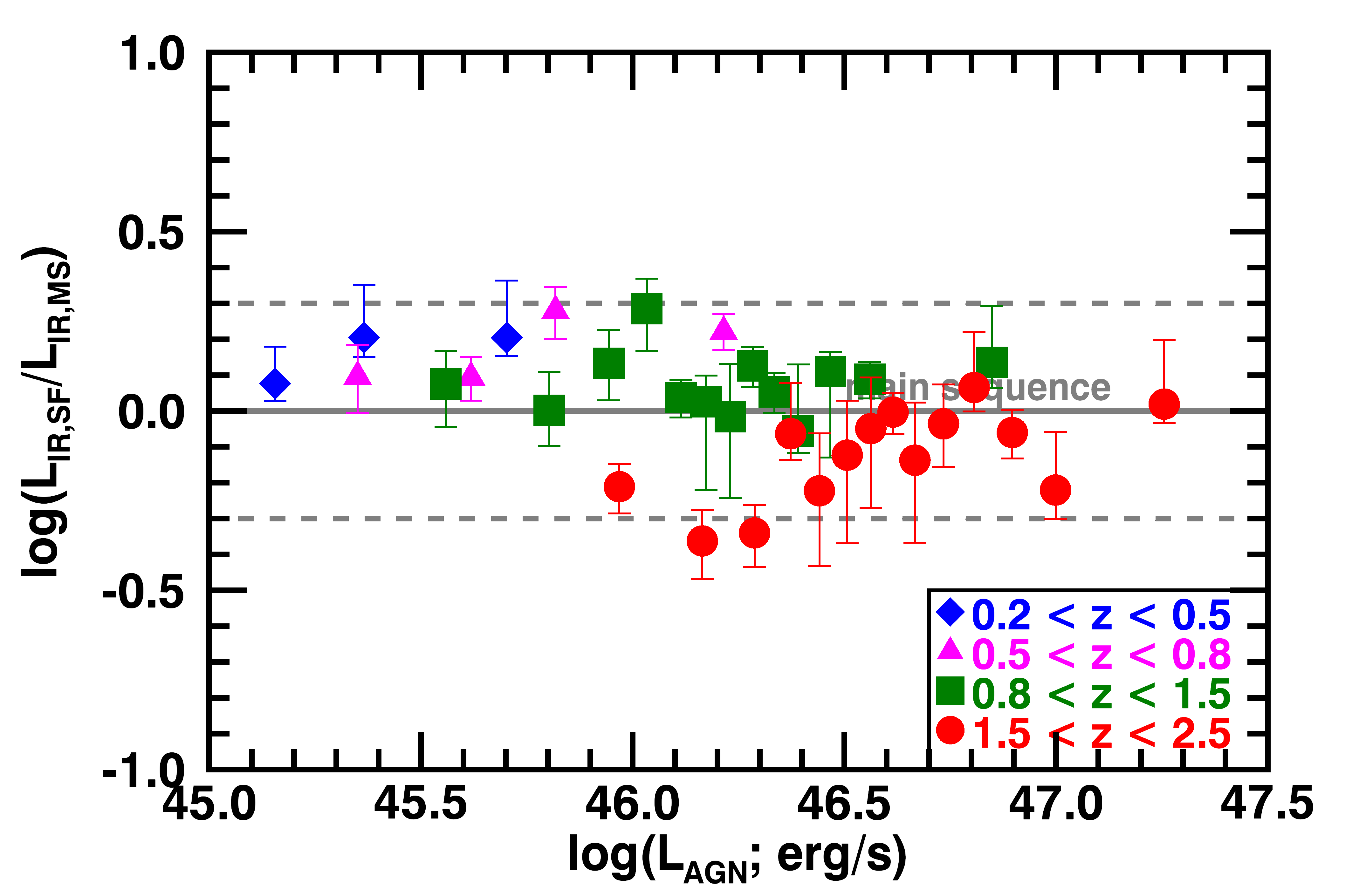
(a)

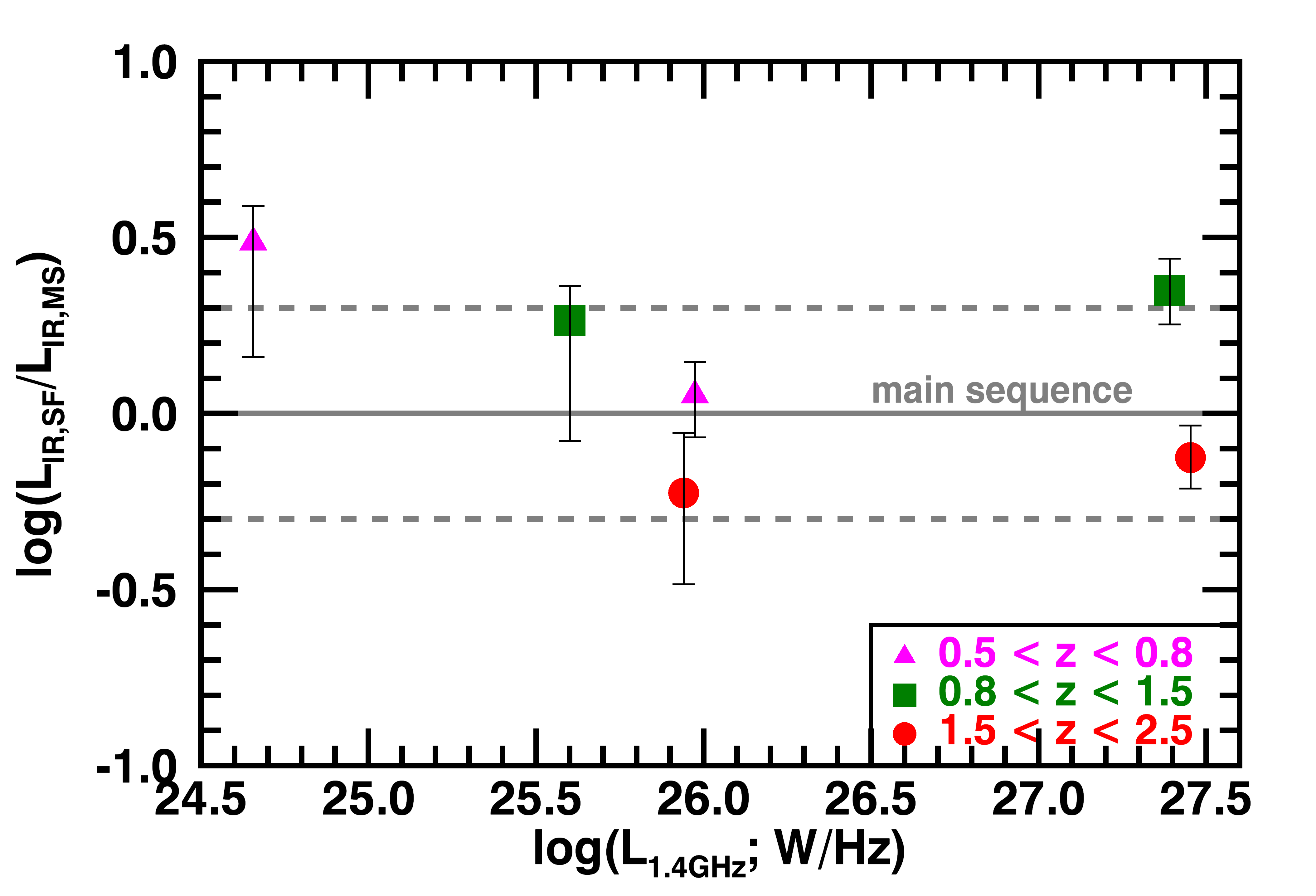
(b)

Figure 12: (a) The ratio of the $\mathrel{\langle L_{\rm IR,SF}\rangle}$ to $\mathrel{\langle L_{\rm IR,MS}\rangle}$ as a function of $\mathrel{L_{\rm AGN,bol}}$. The errors on the ratio are the combination of both the errors on $\mathrel{\langle L_{\rm IR,SF}\rangle}$ and $\mathrel{\langle L_{\rm IR,MS}\rangle}$. The dashed lines indicate a factor of 2 offset, characteristic of the error on the main sequence equation. There is an apparent trend of $\mathrel{\langle L_{\rm IR,SF}\rangle}$/$\mathrel{\langle L_{\rm IR,MS}\rangle}$ with redshift when compared to the main sequence of star-forming galaxies, moving from having comparatively high $\mathrel{\langle L_{\rm IR,SF}\rangle}$ values at low redshifts (0.2$<z<$0.5) to consistent and comparatively low $\mathrel{\langle L_{\rm IR,SF}\rangle}$ values at the highest redshift range of our sample (1.5$<z<$2.5). (b) The ratio of the $\mathrel{\langle L_{\rm IR,SF}\rangle}$ of the radio-luminous QSOs over the $\mathrel{\langle L_{\rm IR,MS}\rangle}$ of the main sequence for galaxies of the same stellar mass and redshift, as a function of $\mathrel{L_{\rm 1.4GHz}}$. We find that the $\mathrel{\langle L_{\rm IR,SF}\rangle}$ of radio-luminous QSOs are consistent with those of main sequence and starbursts galaxies for redshifts of 0.5 $<z<$ 1.5. At higher redshifts of 1.5 $<z<$ 2.5 the radio-luminous QSOs show lower values of $\mathrel{\langle L_{\rm IR,SF}\rangle}$ relative to the main sequence galaxies, in agreement with what we see for the overall sample. We note that, for both the full sample and the radio-luminous QSO sub-sample, the highest redshift range ($1.5<z<2.5$) is affected by the uncertain systematics on deriving the stellar mass, and the choice of AGN template. Consequently, the differences in the results of the highest redshift bin and the rest of the sample should not be over-interpreted (see discussion in section 5.2.1).

In Figure 11 & 12 we plot the results for $\mathrel{\langle L_{\rm IR,MS}\rangle}$ in comparison to the $\mathrel{\langle L_{\rm IR,SF}\rangle}$ of the QSO sample. In Figure 11 we plot $\mathrel{\langle L_{\rm IR,SF}\rangle}$ as a function of $\mathrel{L_{\rm AGN,bol}}$ in comparison to the results for main sequence star-forming galaxies for each redshift range. With the coloured lines we show the $\mathrel{\langle L_{\rm IR,MS}\rangle}$, and the coloured shaded regions correspond to the 1$\sigma$ uncertainty on $\mathrel{\langle L_{\rm IR,MS}\rangle}$ distribution for each bin from our MC calculation. Additionally, we take the ratio of the $\mathrel{\langle L_{\rm IR,SF}\rangle}$ from our analysis over that of the main sequence ($\mathrel{\langle L_{\rm IR,MS}\rangle}$). We show the $\mathrel{\langle L_{\rm IR,SF}\rangle}$/$\mathrel{\langle L_{\rm IR,MS}\rangle}$ ratio as a function of $\mathrel{L_{\rm AGN,bol}}$ in Figure 12(a), propagating the errors of the two variables. With the line we show the expected ratio for the main sequence, while the dashed lines indicate the range covered by the scatter of the main sequence relation as defined by Schreiber et al. (2015). From these two figures we can see an apparent trend in the $\mathrel{\langle L_{\rm IR,SF}\rangle}$ values of QSOs relative to those of the main sequence star-forming galaxies, as a function of redshift. At the highest redshift range of 1.5 $<z<$ 2.5, the $\mathrel{\langle L_{\rm IR,SF}\rangle}$ values are systematically below the main sequence by an average factor of 0.75 (or 1.33 if taking the inverse ratio). Moving to intermediate redshifts of 0.8 $<z<$ 1.5 the $\mathrel{\langle L_{\rm IR,SF}\rangle}$ values become consistent with those of the main sequence, while at redshifts of $z<$ 0.8 the $\mathrel{\langle L_{\rm IR,SF}\rangle}$ values move above those of the main sequence by a factor of 1.5. However, even though some of the means are not consistent within their errors, they are still consistent within the factor of 2 scatter of the main sequence (see Figure 12(a)).

Following the same approach as for the full QSO sample, we estimate the expected IR luminosity of main sequence star-forming galaxies ($\mathrel{\langle L_{\rm IR,MS}\rangle}$) at the same redshift and stellar mass (estimated from the available $\mathrel{M_{\rm BH}}$) for our radio-luminous QSO sample, and compare to their $\mathrel{\langle L_{\rm IR,SF}\rangle}$. In Figure 12(b) we show the $\mathrel{\langle L_{\rm IR,SF}\rangle}$/$\mathrel{\langle L_{\rm IR,MS}\rangle}$ ratio as a function of $\mathrel{L_{\rm AGN,bol}}$. We find that the radio-luminous QSOs have $\mathrel{\langle L_{\rm IR,SF}\rangle}$ values consistent with those of the main sequence within the factor of 2 scatter of the main sequence relation, that show the same redshift dependence as the full sample. Similar results were shown by Drouart et al. (2014) at $z<$ 2.5, following a similar SED fitting approach, for a smaller sample of 70 powerful radio-galaxies from the Herschel radio galaxy evolution sample (HERGÉ). Additionally a number of studies have argued for radio-AGN/QSOs living in star-forming galaxies up to redshifts of $\sim$5 (e.g., Drouart et al. 2014, Rees et al. 2016, Magliocchetti et al. 2016) following a variety of approaches.

The relative offset between our results and the main sequence of star-forming galaxies will be dependent on the M_∗–$\mathrel{M_{\rm BH}}$ relation and redshift evolution assumed. We have performed the same procedure for two other cases of M_∗–$\mathrel{M_{\rm BH}}$ relations with and without redshift evolution. In one case we used the Kormendy & Ho (2013) relation, with no redshift evolution and assuming M${}_{*}\approx\rm M_{bulge}$. In the second case we used the Häring & Rix (2004) relation, following the redshift evolution of Merloni et al. (2010). In both cases the trends of $\mathrel{L_{\rm IR,MS}}$ with $\mathrel{L_{\rm AGN,bol}}$ are similar to those seen when using the Bennert et al. (2011) relation. The $\mathrel{\langle L_{\rm IR,SF}\rangle}$/$\mathrel{L_{\rm IR,MS}}$ values remain within a factor of 1.25 of those estimated with the Bennert et al. (2011) relation, and remain within the factor of 2 scatter of the main sequence. Furthermore, it is also possible for QSOs in our sample to be caught in a phase of having a larger $\mathrel{M_{\rm BH}}$ than that expected by the local M_∗–$\mathrel{M_{\rm BH}}$ relation. However, for this to have a significant impact on the results presented in this section, the majority of the sources in each bin will need to systematically have over-massive BHs, by at least a factor of 2–3. By combining the work of Portinari et al. (2012), that looked into the M_∗–$\mathrel{M_{\rm BH}}$ relation as a function of redshift for QSOs from semi analytical models (SAMs), and the redshift evolution in Eq. 4, we find that the $\mathrel{M_{\rm BH}}$ values could be over-massive by only a factor of $\sim$1.3. Consequently, the $\mathrel{\langle L_{\rm IR,SF}\rangle}$ would still remain within the factor of 2 scatter of the main sequence.

In addition to the above, we note that there is further uncertainty for the comparison to the MS galaxies for our highest redshift range ($1.5<z<2.5$). As shown in section 5.1.2 the highest redshift range is the one most affected by the choice of AGN template. Furthermore, for at least half the sources in this redshift range the BH masses have been estimated from the C IV line, argued to lead to overestimation of the BH mass due to observed blueshifts of the line caused by non-virial processes (see Coatman et al. (2017) and references there-in). For this reason we do not strongly interpret the observed offset of the $\mathrel{\langle L_{\rm IR,SF}\rangle}$ to $\mathrel{L_{\rm IR,MS}}$ for the highest redshift range.

Overall, the $\mathrel{\langle L_{\rm IR,SF}\rangle}$ values of QSOs are consistent with those of main sequence star-forming galaxies within the factor of 2 scatter of the relation. Additionally, the positive trends observed in the $\mathrel{\langle L_{\rm IR,SF}\rangle}$ as a function of $\mathrel{L_{\rm AGN,bol}}$ seem to follow those expected for $\mathrel{\langle L_{\rm IR,MS}\rangle}$ (see Figure 11), suggesting that the observed correlation between $\mathrel{\langle L_{\rm IR,SF}\rangle}$ and $\mathrel{L_{\rm AGN,bol}}$ is primarily driven by the stellar masses and redshifts of the QSOs. We see no evidence for positive or negative AGN feedback as inferred from some previous studies (e.g., Karouzos et al. 2014; Kalfountzou et al. 2014).

5.2.2 The effect of AGN on the star formation of their host galaxies

The results of this study in combination to those of Stanley et al. (2015) are consistent with a scenario where AGN are on average hosted by predominately normal star-forming galaxies (see section 5.2.1). The trends of the mean SFR with $\mathrel{L_{\rm AGN,bol}}$ shown in Figure 9 can be explained by a model where AGN have a broad range of luminosities for a fixed galaxy stellar mass (Aird et al. 2013), due to a stochastic triggering mechanism of AGN and/or AGN variability on shorter timescales than those of star formation (Hickox et al. 2014; also see section 4.3 of Stanley et al. 2015). The transition from a flat trend to a positive trend of the mean SFR with AGN luminosity seen at the highest luminosities, can still be explained with the same scenario (see Figure 11). For such high AGN luminosities, as those of our QSO sample, the range of stellar masses of the host galaxies narrows towards the more massive galaxies that will also contain more cold gas to fuel the AGN and star formation. Consequently, it is not surprising to see an increase in the SFRs of these galaxies. Indeed, in the previous section we have demonstrated that mass effects are driving the observed trends.

However, it is worth noting here that our study has concentrated on HERG type AGN, and we do not consider the possible differences between the two excitation level types in AGN. Gürkan et al. (2015) split AGN at $z<$ 0.6 into LERGs and HERGs, and found that LERGs have lower levels of star formation compared to HERGs. As HERGs and LERGs represent AGN populations with potentially different fuelling mechanisms (e.g., Hardcastle, Evans & Croston 2007; Best & Heckman 2012; Heckman & Best 2014), it is argued that they are hosted by galaxies which are at different stages of their evolution (e.g., Gürkan et al. 2015).

It is likely that any effects of the AGN on star formation are comparatively subtle, and not easily traceable when looking at the mean AGN and galaxy properties. Indeed, using a small number of sources with deep ALMA observations, Mullaney et al. (2015) demonstrated the potential for subtle differences between the SFR distributions of the host galaxies of moderate luminosity AGN, and main sequence star-forming galaxies. Furthermore, the flat trends of SFR with AGN luminosity have been reproduced by the EAGLE simulation (McAlpine et al. 2017), which includes AGN feedback as a crucial component of galaxy evolution (Schaye et al. 2015; Crain et al. 2015). The above results demonstrate that galaxies can show no dependence of their mean SFRs on AGN luminosity, while still being affected by AGN feedback (also see Harrison 2017).

6 Conclusions

The aim of this work has been to constrain the mean SFRs of a sample of $z=$0.2–2.5 QSOs with AGN bolometric luminosities of $10^{45}<\,\mathrel{L_{\rm AGN,bol}}\,<10^{48}\mathrel{\rm erg\;s^{-1}}$. We investigate the mean SFRs as a function of redshift and bolometric AGN luminosity of the whole sample, and a radio-luminous sub-sample with $\mathrel{L_{\rm 1.4GHz}}\,>$ 10${}^{24}\,\hbox{W}\,\hbox{Hz}^{-1}$. We combine the five Herschel bands (100–500$\mathrel{\rm\mu m}$) of the H-ATLAS survey to the MIR bands (12 and 22$\mathrel{\rm\mu m}$) of WISE, and perform SED fitting to the mean fluxes of 34 $\mathrel{L_{\rm AGN,bol}}$–$z$ bins of our full QSO sample, and 6 $\mathrel{L_{\rm 1.4GHz}}$–$z$ bins of the RL-QSO sub-sample. We find that:

• It is important to take into account of AGN contamination in the FIR when calculating the SFRs of QSOs, especially at $z>$ 1.5 where the AGN can cause an overestimation of the SFR by up to a factor of 2–2.5 when derived from the flux density at observed frame 250$\mathrel{\rm\mu m}$ (see Section 4.1).

• The mean SFRs of the optical QSOs show a positive trend with AGN luminosity (see Sections 4.2). We find that this trend is dominated by black-hole mass and redshift dependencies on the IR luminosity due to star formation (see Sections 5.2.1).

• We combine the results of our optical QSO sample to lower AGN luminosity X-ray selected AGN from Stanley et al. (2015), and find that the two samples show consistent mean SFRs at overlapping AGN luminosities, for each redshift range (see Sections 4.2).

• Assuming that the black hole and stellar mass of optical QSOs are correlated, we find that their mean SFRs are consistent to those of main sequence galaxies within the factor of $\sim$2 scatter of the relation. Additionally, the weak positive trend between the mean SFR and AGN luminosity seem to follow those of the main sequence, suggesting that the trends are driven by the mass and redshift dependencies (see Section 5.2.1).

• The radio-luminous QSOs show consistent results to the overall optical QSO sample (see Section 4.3), and are consistent to the main sequence of star-forming galaxies within the factor of 2 scatter of the relation (see Section 5.2.1). However, at luminosities of $\mathrel{\langle L_{\rm 1.4GHz}\rangle}>10^{27}$W/Hz, the $\mathrel{\langle L_{\rm IR,SF}\rangle}$ is highly uncertain due to contamination from Synchrotron radiation (see Section 4.3).

Overall, our results are consistent with a scenario where X-ray and optically selected AGN are hosted on average by normal star-forming galaxies, and show no clear evidence of an increase or decrease of the SFR, on average, due to the presence of the AGN. However, this result cannot rule out a scenario where AGN are responsible for the suppression of star formation, as the timescales for the suppression of star formation may be longer than those of luminous AGN activity (i.e., Harrison 2017). Deeper observations are required to properly constrain the individual source properties of the AGN population. Key progress will be made by combining theoretical predictions with observational constraints on the SFR distributions of AGN to establish the subtle features of AGN feedback, if any.

ACKNOWLEDGMENTS

We thank the anonymous referee for their constructive comments on the paper. We acknowledge the Faculty of Science Durham Doctoral Scholarship (FS), the Science and Technology Facilities Council (DMA, DJR, through grant code ST/L00075X/1), and the Leverhulme Trust (DMA). JA acknowledges support from ERC Advanced Grant FEEDBACK 340442. LD and SJM acknowledge support from the European Research Council Advanced Investigator grant COSMICISM, and also the ERC Consolidator Grant, Cosmic Dust. GDZ acknowledges support from ASI/INAF agreement n. 2014-024-R.1 and by PRIN–INAF 2014 “Probing the AGN/galaxy co-evolution through ultra-deep and ultra-high resolution radio surveys”. M.J.M. acknowledges the support of the National Science Centre, Poland through the POLONEZ grant 2015/19/P/ST9/04010. This project has received funding from the European Union’s Horizon 2020 research and innovation programme under the Marie Skłodowska-Curie grant agreement No. 665778.

The Herschel-ATLAS is a project with Herschel, which is an ESA space observatory with science instruments provided by European-led Principal Investigator consortia and with important participation from NASA. The H-ATLAS web-site is http://www.h-atlas.org¡http://atlas.org¿.

Appendix A SED fits for all bins

In this Appendix section we present the best-fit SEDs for all bins in our sample. In Figure A.1 we show the best-fits of each bin for our full QSO sample, with IDs that correspond to those of Table 1. In Figure A.2 we show the best-fits for our radio-luminous sub-sample, with IDs that correspond to those of Table 2.

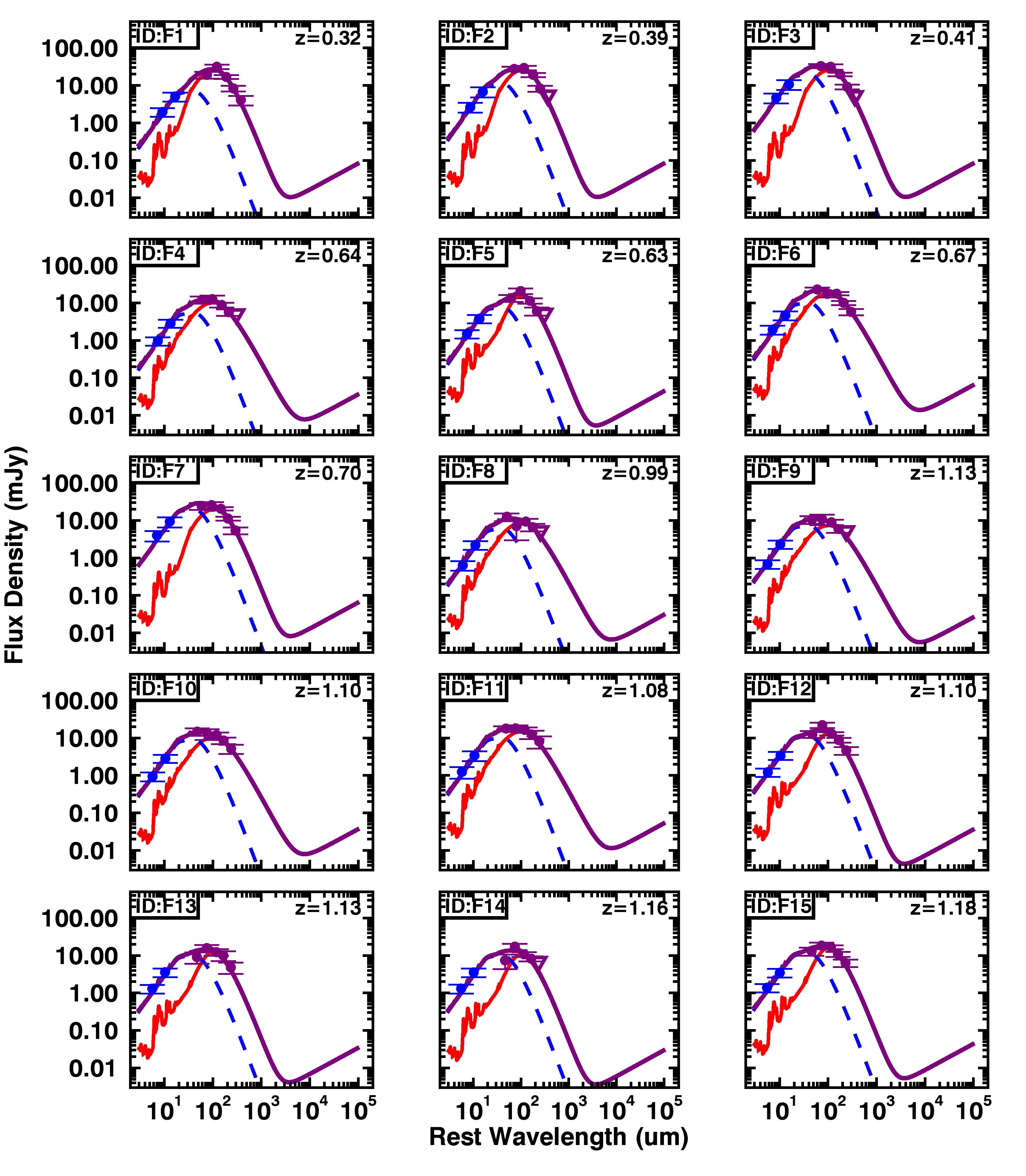
Figure A.1: The best-fit SEDs for all the $z$–$\mathrel{L_{\rm AGN,bol}}$ bins of the QSO sample. The data points correspond to the mean photometry of each bin and the downwards pointing triangles correspond to the upper limits. The blue dashed curve is the AGN component of the SED, while the red solid curve is the SF component, and the purple solid curve corresponds to the total IR SED. The ID name corresponds to that of Table 1 for direct reference, and the redshift corresponds to the mean redshift of the sources in the $z$–$\mathrel{L_{\rm AGN,bol}}$ bin.

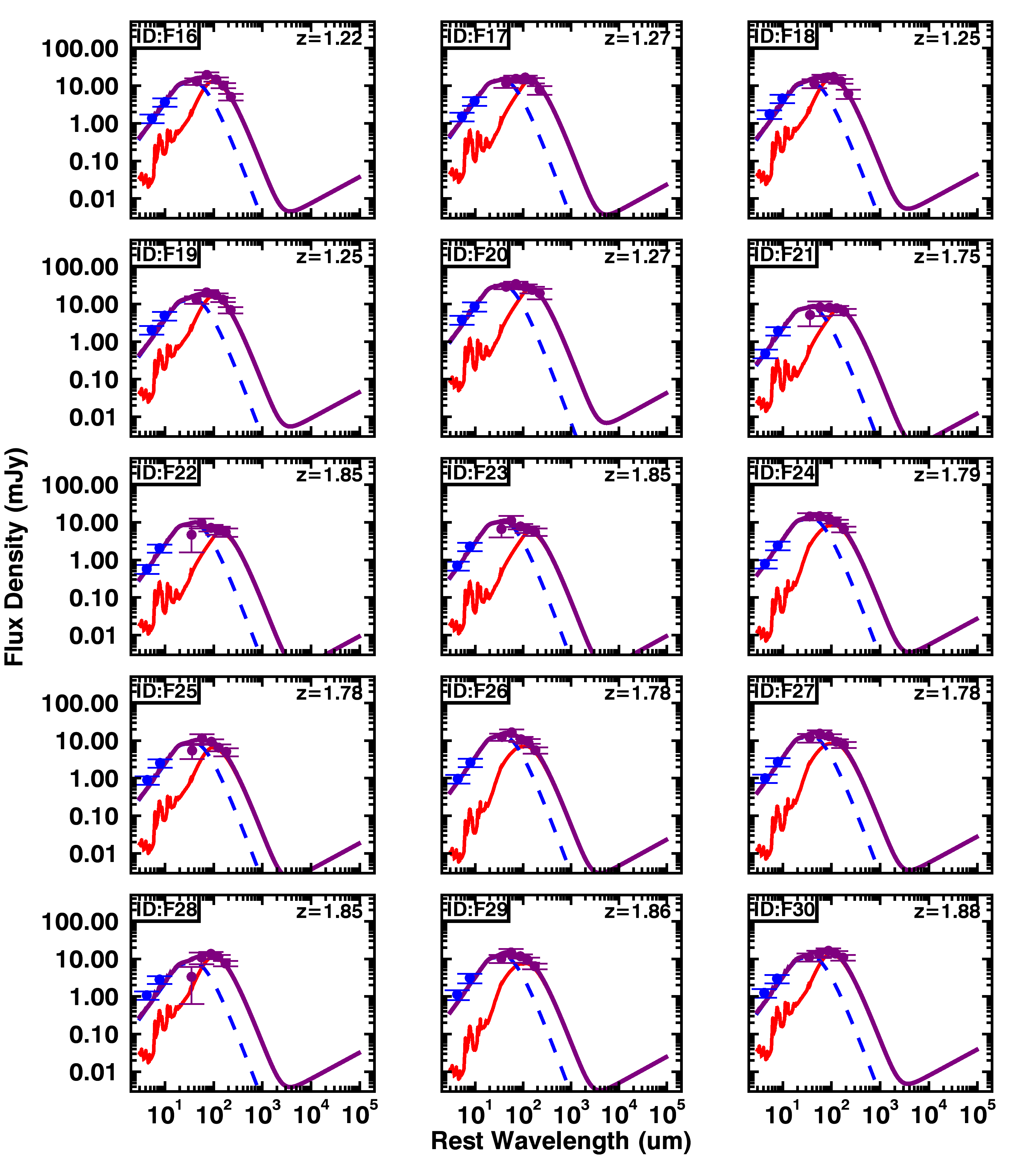
Figure A.1: Continued

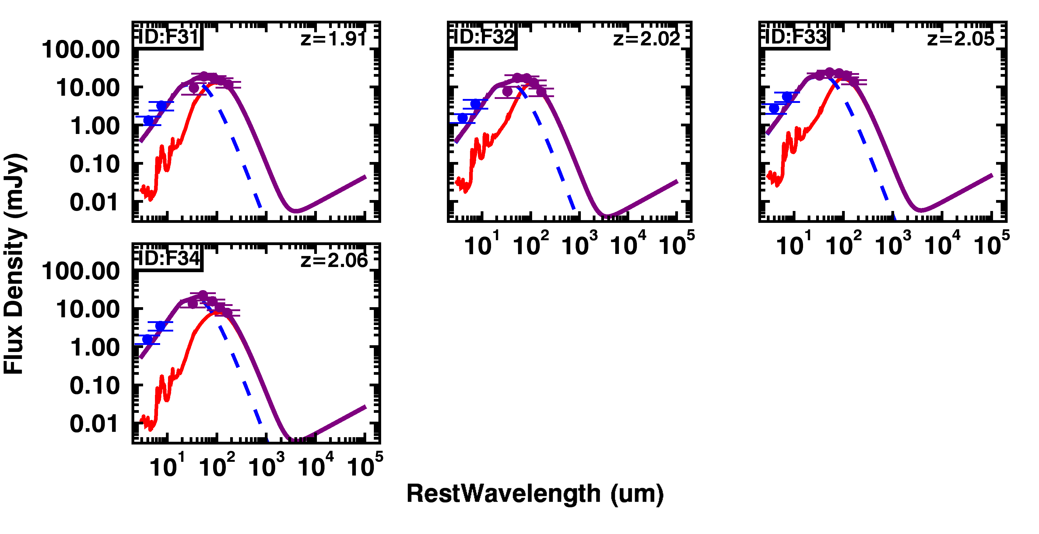
Figure A.1: Continued

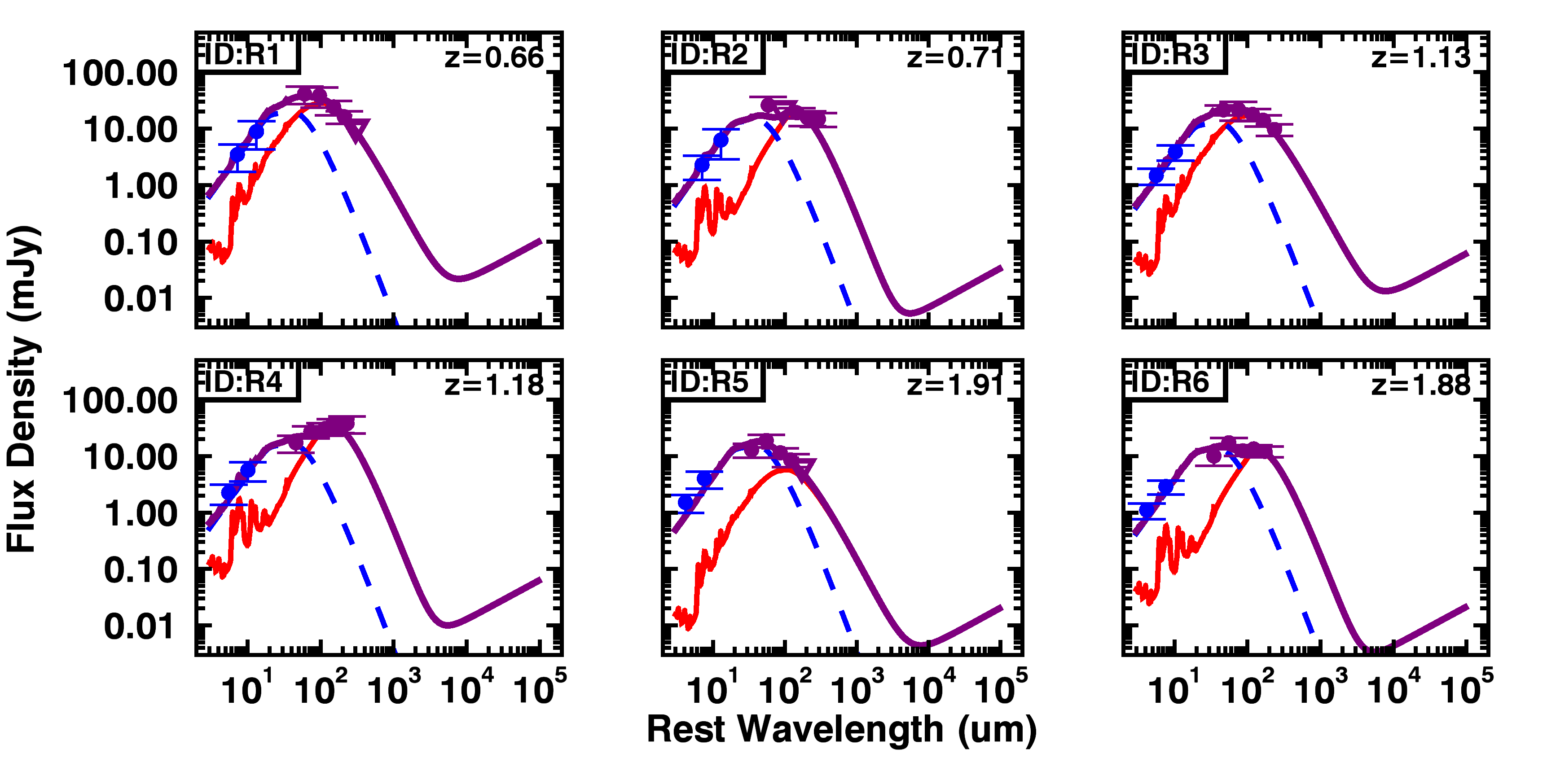
Figure A.2: The best-fit SEDs for all the $z$–$\mathrel{L_{\rm 1.4GHz}}$ bins of the RL–QSO sample. The data points correspond to the mean photometry of each bin and the downwards pointing triangles correspond to the upper limits. The blue dashed curve is the AGN component of the SED, while the red solid curve is the SF component, and the purple solid curve corresponds to the total IR SED. The IDs correspond to those of Table 2 for direct reference, and the redshift corresponds to the mean redshift of the sources in the $z$–$\mathrel{L_{\rm 1.4GHz}}$ bin..

Appendix B The radial light profile of SPIRE stacked sources

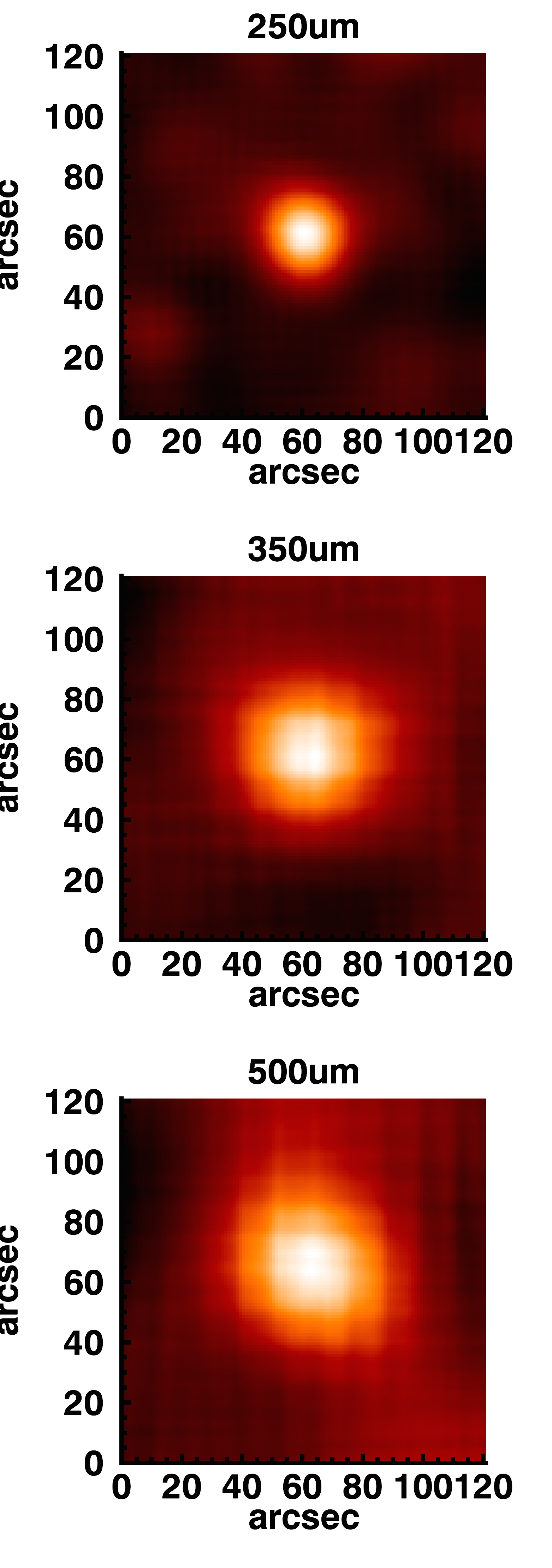
(a)

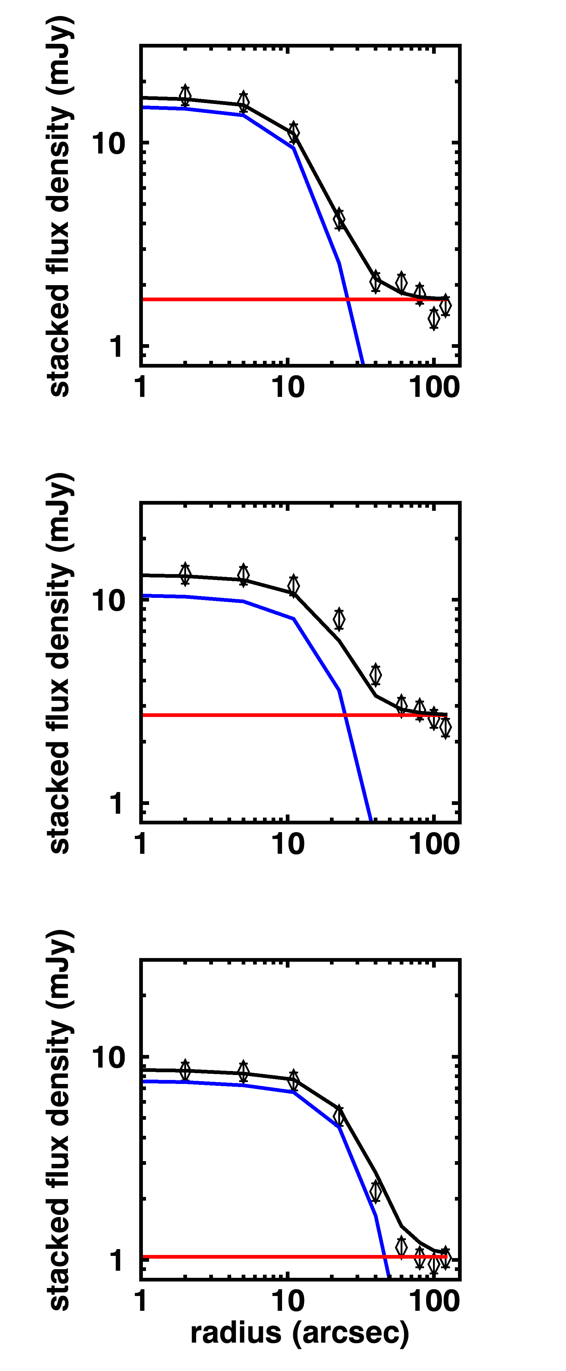
(b)

Figure B.3: Examples of our radial light profile analysis for the three SPIRE bands. In the left-hand panels are the stacked images in 250$\mathrel{\rm\mu m}$, 350$\mathrel{\rm\mu m}$ and 500$\mathrel{\rm\mu m}$. In the right-hand panel we show examples of the radial light profile of the stacked image used to estimate the contamination from bright neighbouring sources. The light profile is fitted with the convolved PSF (blue) for each band respectively, and a constant flux density level fitted to the high end tail for the estimation of the contamination factor to the stacked flux density (red).

An additional cause for uncertainty in the SPIRE stacked flux density estimates is the possible boosting due to nearby sources. QSOs are well known to be clustered (e.g., White et al. 2012 and references therein), and in Wang et al. (2015) it was found that due to the clustering of other dusty star-forming galaxies around optical QSOs there is a $\sim$ 8–13% contamination to the 250$\mathrel{\rm\mu m}$–500$\mathrel{\rm\mu m}$ flux density, respectively. To take this possible source of contamination into account, we measure the average flux density in annuli, and fit the flux density as a function of radius from the center to a radius of $\sim$ 150$"$. We use the SPIRE PSF (provided by H-ATLAS) convolved with itself, which corresponds to the images we are using, and a constant flux density level that is free to vary (see last panel in Figure B.3). The factor of contamination calculated for each bin shows no dependency on redshift and AGN luminosity, and has a median of $\sim$11% at 250$\mathrel{\rm\mu m}$, 24% at 350$\mathrel{\rm\mu m}$, and 14% at 500$\mathrel{\rm\mu m}$. However, the absolute values of the contamination factor are equivalent to the offset that we see in the random stack distribution, which we have used when correcting the stacked flux densities. Consequently, the contamination measured here is still only constraining the confusion background of our fits, and there may be an additional contamination factor due to clustering that we can not constrain here.

References

- Aird et al. (2012) Aird J. et al., 2012, ApJ, 746, 90
- Aird et al. (2013) Aird J. et al., 2013, ApJ, 775, 41
- Alexander & Hickox (2012) Alexander D. M., Hickox R. C., 2012, NAR, 56, 93
- Azadi et al. (2015) Azadi M. et al., 2015, ApJ, 806, 187
- Becker, White & Helfand (1995) Becker R. H., White R. L., Helfand D. J., 1995, ApJ, 450, 559
- Bennert et al. (2011) Bennert V. N., Auger M. W., Treu T., Woo J.-H., Malkan M. A., 2011, ApJ, 742, 107
- Best & Heckman (2012) Best P. N., Heckman T. M., 2012, MNRAS, 421, 1569
- Bonfield et al. (2011) Bonfield D. G. et al., 2011, MNRAS, 416, 13
- Bourne et al. (2016) Bourne N. et al., 2016, MNRAS, 462, 1714
- Bower et al. (2006) Bower R. G., Benson A. J., Malbon R., Helly J. C., Frenk C. S., Baugh C. M., Cole S., Lacey C. G., 2006, MNRAS, 370, 645
- Bruzual & Charlot (2003) Bruzual G., Charlot S., 2003, MNRAS, 344, 1000
- Calzetti et al. (2010) Calzetti D. et al., 2010, ApJ, 714, 1256
- Casey, Narayanan & Cooray (2014) Casey C. M., Narayanan D., Cooray A., 2014, Physics Reports, 541, 45
- Chabrier (2003) Chabrier G., 2003, PASP, 115, 763
- Coatman et al. (2017) Coatman L., Hewett P. C., Banerji M., Richards G. T., Hennawi J. F., Prochaska J. X., 2017, MNRAS, 465, 2120
- Crain et al. (2015) Crain R. A. et al., 2015, MNRAS, 450, 1937
- Del Moro et al. (2013) Del Moro A. et al., 2013, A&A, 549, A59
- Delvecchio et al. (2014) Delvecchio I. et al., 2014, MNRAS, 439, 2736
- Di Matteo, Springel & Hernquist (2005) Di Matteo T., Springel V., Hernquist L., 2005, Nature, 433, 604
- Domínguez Sánchez et al. (2014) Domínguez Sánchez H. et al., 2014, MNRAS, 441, 2
- Drouart et al. (2014) Drouart G. et al., 2014, A&A, 566, A53
- Drouart et al. (2016) Drouart G., Rocca-Volmerange B., De Breuck C., Fioc M., Lehnert M., Seymour N., Stern D., Vernet J., 2016, A&A, 593, A109
- Eales et al. (2010) Eales S. et al., 2010, PASP, 122, 499
- Elbaz et al. (2007) Elbaz D. et al., 2007, A&A, 468, 33
- Elbaz et al. (2011) Elbaz D. et al., 2011, A&A, 533, A119
- Fabian (2012) Fabian A. C., 2012, ARAA, 50, 455
- Feigelson & Nelson (1985) Feigelson E. D., Nelson P. I., 1985, ApJ, 293, 192
- Genel et al. (2014) Genel S. et al., 2014, MNRAS, 445, 175
- Gürkan et al. (2015) Gürkan G. et al., 2015, MNRAS, 452, 3776
- Hardcastle et al. (2013) Hardcastle M. J. et al., 2013, MNRAS, 429, 2407
- Hardcastle, Evans & Croston (2007) Hardcastle M. J., Evans D. A., Croston J. H., 2007, MNRAS, 376, 1849
- Häring & Rix (2004) Häring N., Rix H.-W., 2004, ApJL, 604, L89
- Harris et al. (2016) Harris K. et al., 2016, MNRAS, 457, 4179
- Harrison (2017) Harrison C. M., 2017, Nature Astronomy, 1, 0165
- Harrison et al. (2012) Harrison C. M. et al., 2012, ApJL, 760, L15
- Heckman & Best (2014) Heckman T. M., Best P. N., 2014, ARAA, 52, 589
- Hickox et al. (2014) Hickox R. C., Mullaney J. R., Alexander D. M., Chen C.-T. J., Civano F. M., Goulding A. D., Hainline K. N., 2014, ApJ, 782, 9
- Kalfountzou et al. (2014) Kalfountzou E. et al., 2014, MNRAS, 442, 1181
- Karouzos et al. (2014) Karouzos M. et al., 2014, ApJ, 784, 137
- Kellermann et al. (1989) Kellermann K. I., Sramek R., Schmidt M., Shaffer D. B., Green R., 1989, AJ, 98, 1195
- Kennicutt (1998) Kennicutt, Jr. R. C., 1998, ARAA, 36, 189
- Kormendy & Ho (2013) Kormendy J., Ho L. C., 2013, ARAA, 51, 511
- Lani, Netzer & Lutz (2017) Lani C., Netzer H., Lutz D., 2017, arXiv:1705.0674
- Lanzuisi et al. (2017) Lanzuisi G. et al., 2017, A&A, 602, A123
- Liddle (2004) Liddle A. R., 2004, MNRAS, 351, L49
- Lutz (2014) Lutz D., 2014, ARAA, 52, 373
- Lyu & Rieke (2017) Lyu J., Rieke G. H., 2017, ApJ, 841, 76
- Magliocchetti et al. (2014) Magliocchetti M. et al., 2014, MNRAS, 442, 682
- Magliocchetti et al. (2016) Magliocchetti M., Lutz D., Santini P., Salvato M., Popesso P., Berta S., Pozzi F., 2016, MNRAS, 456, 431
- Magnelli et al. (2014) Magnelli B. et al., 2014, A&A, 561, A86
- McAlpine, Jarvis & Bonfield (2013) McAlpine K., Jarvis M. J., Bonfield D. G., 2013, MNRAS, 436, 1084
- McAlpine et al. (2017) McAlpine S., Bower R. G., Harrison C. M., Crain R. A., Schaller M., Schaye J., Theuns T., 2017, MNRAS, 468, 3395
- Merloni et al. (2010) Merloni A. et al., 2010, ApJ, 708, 137
- Mor & Netzer (2012) Mor R., Netzer H., 2012, MNRAS, 420, 526
- Mullaney et al. (2015) Mullaney J. R. et al., 2015, MNRAS, 453, L83
- Mullaney et al. (2011) Mullaney J. R., Alexander D. M., Goulding A. D., Hickox R. C., 2011, MNRAS, 414, 1082
- Mullaney et al. (2012) Mullaney J. R. et al., 2012, MNRAS, 419, 95
- Netzer et al. (2016) Netzer H., Lani C., Nordon R., Trakhtenbrot B., Lira P., Shemmer O., 2016, ApJ, 819, 123
- Netzer et al. (2007) Netzer H. et al., 2007, ApJ, 666, 806
- Noeske et al. (2007) Noeske K. G. et al., 2007, ApJL, 660, L43
- Page et al. (2012) Page M. J. et al., 2012, Nature, 485, 213
- Pannella et al. (2015) Pannella M. et al., 2015, ApJ, 807, 141
- Pilbratt et al. (2010) Pilbratt G. L. et al., 2010, A&A, 518, L1
- Pineau et al. (2011) Pineau F.-X., Motch C., Carrera F., Della Ceca R., Derrière S., Michel L., Schwope A., Watson M. G., 2011, A&A, 527, A126
- Pitchford et al. (2016) Pitchford L. K. et al., 2016, MNRAS, 462, 4067
- Podigachoski et al. (2016) Podigachoski P., Rocca-Volmerange B., Barthel P., Drouart G., Fioc M., 2016, MNRAS, 462, 4183
- Portinari et al. (2012) Portinari L., Kotilainen J., Falomo R., Decarli R., 2012, MNRAS, 420, 732
- Rees et al. (2016) Rees G. A. et al., 2016, MNRAS, 455, 2731
- Richards et al. (2006) Richards G. T. et al., 2006, ApJS, 166, 470
- Rosario et al. (2016) Rosario D. J., Mendel J. T., Ellison S. L., Lutz D., Trump J. R., 2016, MNRAS, 457, 2703
- Rosario et al. (2012) Rosario D. J. et al., 2012, A&A, 545, A45
- Rosario et al. (2013) Rosario D. J. et al., 2013, A&A, 560, A72
- Schaye et al. (2015) Schaye J. et al., 2015, MNRAS, 446, 521
- Schneider et al. (2010) Schneider D. P. et al., 2010, AJ, 139, 2360
- Schneider et al. (2015) Schneider R., Bianchi S., Valiante R., Risaliti G., Salvadori S., 2015, A&A, 579, A60
- Schreiber et al. (2015) Schreiber C. et al., 2015, A&A, 575, A74
- Schwarz (1978) Schwarz G., 1978, The Annals of Statistics, 6, 461
- Serjeant et al. (2010) Serjeant S. et al., 2010, A&A, 518, L7
- Seymour et al. (2011) Seymour N. et al., 2011, MNRAS, 413, 1777
- Shen et al. (2011) Shen Y. et al., 2011, ApJS, 194, 45
- Silva et al. (1998) Silva L., Granato G. L., Bressan A., Danese L., 1998, ApJ, 509, 103
- Stanley et al. (2015) Stanley F., Harrison C. M., Alexander D. M., Swinbank A. M., Aird J. A., Del Moro A., Hickox R. C., Mullaney J. R., 2015, MNRAS, 453, 591
- Stern et al. (2012) Stern D. et al., 2012, ApJ, 753, 30
- Symeonidis et al. (2016) Symeonidis M., Giblin B. M., Page M. J., Pearson C., Bendo G., Seymour N., Oliver S. J., 2016, MNRAS
- Thacker et al. (2014) Thacker R. J., MacMackin C., Wurster J., Hobbs A., 2014, MNRAS, 443, 1125
- Valiante et al. (2016) Valiante E. et al., 2016, MNRAS, 462, 3146
- Volonteri et al. (2015) Volonteri M., Capelo P. R., Netzer H., Bellovary J., Dotti M., Governato F., 2015, MNRAS, 449, 1470
- Wang et al. (2015) Wang L. et al., 2015, MNRAS, 449, 4476
- Whitaker et al. (2012) Whitaker K. E., van Dokkum P. G., Brammer G., Franx M., 2012, ApJL, 754, L29
- White et al. (2012) White M. et al., 2012, MNRAS, 424, 933
- Wright et al. (2010) Wright E. L. et al., 2010, AJ, 140, 1868