Distribution functions for resonantly trapped orbits in the Galactic disc

Abstract

The present-day response of a Galactic disc stellar population to a non-axisymmetric perturbation of the potential has previously been computed through perturbation theory within the phase-space coordinates of the unperturbed axisymmetric system. Such an Eulerian linearized treatment however leads to singularities at resonances, which prevent quantitative comparisons with data. Here, we manage to capture the behaviour of the distribution function (DF) at a resonance in a Lagrangian approach, by averaging the Hamiltonian over fast angle variables and re-expressing the DF in terms of a new set of canonical actions and angles variables valid in the resonant region. We then follow the prescription of Binney (2016), assigning to the resonant DF the time average along the orbits of the axisymmetric DF expressed in the new set of actions and angles. This boils down to phase-mixing the DF in terms of the new angles, such that the DF for trapped orbits only depends on the new set of actions. This opens the way to quantitatively fitting the effects of the bar and spirals to Gaia data in terms of distribution functions in action space.

1 Introduction

The optimal exploitation of the next data releases of the Gaia mission (Gaia Collaboration et al., 2016) will necessarily involve the construction of a fully dynamical model of the Milky Way. Rather than trying to construct a quixotic full ab initio hydrodynamical model of the Galaxy, which would never be able to reproduce all the details of the Gaia data, a promising approach is to rather construct a multi-component phase-space distribution function (DF) representing each stellar population as well as dark matter, and to compute the potential that these populations jointly generate (e.g., Binney & Piffl, 2015). To do so, one can make use of Jeans theorem, constraining the DF of an equilibrium configuration to depend only on three integrals of motion. Choosing three integrals of motion which have canonically conjugate variables, allows us to express the Hamiltonian $H_{0}$ in its simplest form, i.e. depending only on these three integrals. Such integrals are called the “action variables” $\boldsymbol{J}$, and are new generalized momenta having the dimension of velocity times distance, while their dimensionless canonically conjugate variables are called the “angle variables” $\boldsymbol{\theta}$, because they are usually normalized such that the phase-space position is $2\pi$-periodic in them (e.g. Binney & Tremaine, 2008). In absence of perturbations, these angles evolve linearly with time, $\boldsymbol{\theta}(t)=\boldsymbol{\theta}_{0}+\boldsymbol{\Omega}t$, where $\boldsymbol{\Omega}(\boldsymbol{J})\equiv\partial H_{0}/\partial\boldsymbol{J}$ is the vector of fundamental orbital frequencies. In an equilibrium configuration, the angle coordinates of stars are phase-mixed on orbital tori that are defined by the actions $\boldsymbol{J}$ alone, and the phase-space density of stars $f_{0}(\boldsymbol{J})\mathrm{d}^{3}\boldsymbol{J}$ corresponds to the number of stars $\mathrm{d}N$ in a given infinitesimal action range divided by $(2\pi)^{3}$. In an axisymmetric configuration, the action variables can simply be chosen to be the radial, azimuthal and vertical actions respectively. By constructing DFs depending on these action variables, the current best axisymmetric models of the Milky Way have been constructed (Cole & Binney, 2017).

The Milky Way is however not axisymmetric: it harbours both a bar (de Vaucouleurs, 1964; Binney et al., 1991, 1997; Wegg et al., 2015; Monari et al., 2017a, b) and spiral arms, the exact number, dynamics and nature of which are still under debate (Sellwood & Carlberg, 2014; Grand et al., 2015). Whilst Trick et al. (2017) showed that spiral arms might not affect the axisymmetric fit, the combined effects of spiral arms and the central bar of the Milky Way are clearly important observationally (e.g., McMillan, 2013; Bovy et al., 2015). Hence, non-axisymmetric distribution functions are needed to pin down the present structure of the non-axisymmetric components of the potential, which have enormous importance as drivers of the secular evolution of the disc (Fouvry et al., 2015a, c; Aumer et al., 2016; Aumer & Binney, 2017).

A recent step (Monari et al., 2016a) has been to derive from perturbation theory explicit distribution functions for present-day snapshots of the disc as a function of the actions and angles of the unperturbed axisymmetric system. This work, which is an Eulerian approach to the problem posed by non-axisymmetry, has allowed us to probe the effect of stationary spiral arms in three spatial dimensions, away from the main resonances. In particular, the moments of the perturbed distribution function describe “breathing” modes of the Galactic disc in perfect accordance with simulations (Monari et al., 2016a). Such a breathing mode might actually have been detected in the extended Solar neighbourhood (Williams et al., 2013), but with a larger amplitude, perhaps because the spiral arms are transient. Although such an Eulerian treatment has also been used to gain qualitative insights on the effects of non-axisymmetries near resonances (Monari et al., 2017a), no quantitative assessments can be made with such an approach, because the linear treatment diverges at resonances (the problem of small divisors, Binney & Tremaine, 2008).

In the present contribution, we solve this problem by developing the Lagrangian approach to the impact of non-axisymmetries at resonances. The basic idea is to model the deformation of the orbital tori outside of the trapping region, and to construct new tori, complete with a new system of angle-action variables, within the trapping region (Kaasalainen, 1994). Finally, following Binney (2016) we populate the new tori by phase-averaging the unperturbed distribution function over the new tori.

In Section 2, we present some examples of trapped and untrapped orbits. In Section 3, we summarise the standard approach to a resonance, namely to make a canonical transformation to fast and slow angles and actions, and to replace the real Hamiltonian by its average over the fast angles (Arnold, 1978). Under this averaged Hamiltonian the slow variables have the dynamics of a pendulum. In Section 4, we introduce the pendulum’s angles and actions. In Section 5, we discuss how to build the distribution function using the newly introduced pendulum angles and actions, both inside and outside the zone of trapping at resonances. In Section 6, we present the form of the distribution functions in velocity space, in cases of astrophysical interest related to the Galactic bar. We conclude in Section 7.

2 The bar and trapped orbits

Let us consider orbits in the Galactic plane, and let $(R,\phi)$ be the Galactocentric radius and azimuth. The logarithmic potential, corresponding to a flat circular velocity curve $v_{\mathrm{c}}(R)=v_{0}$, is a rough but simple representation of the potential of the Galaxy. In a formula,

$$\Phi(R)=v_{0}^{2}\ln(R/R_{0}),$$ (1)

with $R_{0}$ the distance of the Sun from the Galactic center. Motion in this planar axisymmetric potential admits actions $J_{\phi}$, which is simply the angular momentum about the Galactic centre, and $J_{R}$, which quantifies the extent of radial oscillations.

Let the axisymmetric potential be perturbed by a non axisymmetric component

$$\Phi_{1}(R,\phi,t)=\operatorname{Re}\left\{\Phi_{\mathrm{a}}(R)\mathrm{e}^{\mathrm{i}m(\phi-\Omega_{\mathrm{b}}t)}\right\},$$ (2)

where $\Omega_{\mathrm{b}}$ is the pattern speed. We will specialise to the bar adopted by Dehnen (2000) and Monari et al. (2017a), so we set $m=2$ and adopt

$$\Phi_{\mathrm{a}}(R)=-\alpha_{\mathrm{b}}\frac{R_{0}^{5}\Omega_{0}^{2}}{3R_{\mathrm{b}}^{3}}\times\left\{\begin{array}[]{l l}(R/R_{\mathrm{b}})^{-3}&\quad\text{}R\geq R_{\mathrm{b}},\\ 2-(R/R_{\mathrm{b}})^{3}&\quad\text{}R<R_{\mathrm{b}},\end{array}\right.$$ (3)

where $\Omega_{0}\equiv\Omega(R_{0})$ is the circular frequency at the solar radius, $R_{\mathrm{b}}$ is the length of the bar and $\alpha_{\mathrm{b}}$ represents the maximum ratio between the radial force contributed by the bar and the axisymmetric background at the Sun (see also Monari et al., 2015, 2016b). We further set $R_{0}=8.2\,\mathrm{kpc}$, $v_{0}=243\,\mathrm{km}\,\mathrm{s}^{-1}$, $R_{\mathrm{b}}=3.5\,\mathrm{kpc}$, and $\alpha=0.01$,

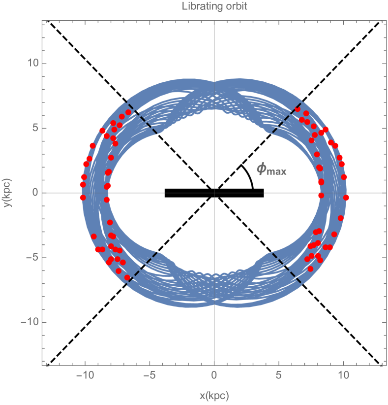
Figure 1: Two orbits in the Galactic potential described in this work, shown in the reference frame corotating with the bar. Here, the pattern speed is chosen to be $\Omega_{\mathrm{b}}=1.8\Omega_{0}$. The red points correspond to the position of the relative apocentres. The thick horizontal line represents the long axis of the bar. The bar rotates counterclockwise. Left panel: an orbit trapped to the outer Lindblad resonance, where the angle $\phi_{\mathrm{max}}$ (dashed lines) represents the maximum extension of the apocentres excursions. Right panel: a circulating orbit.

Fig. 1 shows for $\Omega_{\mathrm{b}}=1.8\Omega_{0}$ two orbits in the reference frame corotating with the bar. The red points in this plot correspond to the relative apocentres of the orbit. In the left panel of Fig. 1, the azimuths of the apocentre points do not cover the whole $[0,2\pi]$ range, but rather oscillate within the interval $[-\phi_{\mathrm{max}},\phi_{\mathrm{max}}]$. The orbit is said to be “trapped” at a resonance, in this case the outer Lindblad resonance (see below), and the angle of the apocentres, the “precession angle”, is said to “librate”. For comparison, the right panel of Fig. 1 shows an orbit for which the precession angle covers the whole $[0,2\pi]$ range. This orbit is said to “circulate”. In the following, we give a quantitative description of these two types of orbits, using perturbation theory.

3 Reduction to a pendulum

We will hereafter work within the epicyclic approximation (Binney & Tremaine, 2008), in which radial oscillations are harmonic with angular frequency $\kappa(R)$, so the radial action $J_{R}=E_{R}/\kappa$, where $E_{R}=E-E_{\mathrm{c}}$ is the energy of these oscillations ($E_{\mathrm{c}}$ being the energy of a circular orbit with the same angular momentum $J_{\phi}$). Using the formulae reported in Dehnen (1999) and Monari et al. (2017a), we can then relate the coordinates of the trapped orbit to the angles $\theta_{R}$ and $\theta_{\phi}$ of the unperturbed system. We can also rewrite the perturbing potential in the Galactic plane in terms of actions and angles as a Fourier series

$$\Phi_{1}(J_{R},J_{\phi},\theta_{R},\theta_{\phi})=\operatorname{Re}\Bigg{\{}\sum_{j=-1}^{1}c_{jm}\mathrm{e}^{\mathrm{i}\left[j\theta_{R}+m\left(\theta_{\phi}-\Omega_{\mathrm{b}}t\right)\right]}\Bigg{\}},$$ (4)

with

$$c_{jm}(J_{R},J_{\phi}) \equiv\Bigg{[}\delta_{j0}+\delta_{|j|1}\frac{m}{2}\mathrm{sgn}(j)\gamma e\Bigg{]}\Phi_{\mathrm{a}}(R_{\mathrm{g}},0)$$

$$\quad-\delta_{|j|1}\frac{R_{\mathrm{g}}}{2}e\frac{\partial\Phi_{\mathrm{a}}}{\partial R}(R_{\mathrm{g}},0).$$ (5)

Here the guiding radius $R_{\mathrm{g}}(J_{\phi})$ is defined by $R_{\mathrm{g}}^{2}\Omega(R_{\mathrm{g}})=J_{\phi}$, the eccentricity by $e(J_{R},J_{\phi})=\sqrt{2J_{R}/(\kappa R_{\mathrm{g}}^{2})}$, and $\gamma=2\Omega(R_{\mathrm{g}})/\kappa(R_{\mathrm{g}})$. In the epicyclic approximation, the radial and azimuthal frequencies of an orbit of actions $(J_{R},J_{\phi})$ are $\Omega_{R}=\kappa(R_{\mathrm{g}})$, and $\Omega_{\phi}=\Omega(R_{\mathrm{g}})+[\mathrm{d}\kappa(R_{\mathrm{g}})/\mathrm{d}J_{\phi}]J_{R}$.

At a resonance, the orbital frequencies $\Omega_{R}$ and $\Omega_{\phi}$ satisfy

$$l\Omega_{R}+m(\Omega_{\phi}-\Omega_{\mathrm{b}})=0.$$ (6)

The three main resonances are the corotation resonance ($l=0$), and the outer ($l=1$) and inner ($l=-1$) Lindblad resonances. To capture the behaviour of the slow and fast varying motions near the resonances, one makes a canonical transformation of coordinates defined by the following time-dependent generating function of type 2 (e.g., Weinberg, 1994)

$$S(\theta_{R},\theta_{\phi},J_{\mathrm{s}},J_{\mathrm{f}},t)=\left[l\theta_{R}+m\left(\theta_{\phi}-\Omega_{\mathrm{b}}t\right)\right]J_{\mathrm{s}}+\theta_{R}J_{\mathrm{f}}.$$ (7)

The new angles and actions $(\theta_{\mathrm{f}},\theta_{\mathrm{s}},J_{\mathrm{f}},J_{\mathrm{s}})$ are then related to the old ones by

$$\theta_{\mathrm{s}} =l\theta_{R}+m\left(\theta_{\phi}-\Omega_{\mathrm{b}}t\right),\quad J_{\phi} =mJ_{\mathrm{s}},$$ (8)

$$\theta_{\mathrm{f}} =\theta_{R},\quad J_{R} =lJ_{\mathrm{s}}+J_{\mathrm{f}}.$$

By taking the time-derivative of $\theta_{\mathrm{s}}$ in the unperturbed system, and by the definition of the resonance in Eq. 6, one finds that the evolution of the new “slow” angle $\theta_{\mathrm{s}}$ is indeed slow near a resonance. Given that along nearly circular orbits $\theta_{\phi}\simeq\phi$, from Eq. (8) we can understand why $\theta_{\mathrm{s}}$ represents the azimuth of the apocentres and pericentres of the orbit in the frame of reference that corotates with the bar: at $\theta_{R}=0$ ($\theta_{R}=-\pi$), we are at the pericentre (apocentre) of the orbit and $\theta_{\mathrm{s}}$ ($\theta_{\mathrm{s}}+\pi$) is $m$ times the star’s azimuth $\theta_{\phi}-\Omega_{\mathrm{b}}t$ in the frame of reference corotating with the orbit.

In the new canonical coordinates of Eq. (8), the motion in the perturbed system is described by the following Hamiltonian (also called the Jacobi integral)

$$H=H_{0}+\operatorname{Re}\left\{\sum_{j=-1}^{1}c_{jm}\mathrm{e}^{\mathrm{i}\left[(j-l)\theta_{\mathrm{f}}+\theta_{\mathrm{s}}\right]}\right\}-m\Omega_{\mathrm{b}}J_{\mathrm{s}},$$ (9)

where $H_{0}$ is the Hamiltonian of the unperturbed axisymmetric system and the $c_{jm}$ coefficients are the Fourier coefficients from Eq. (3), expressed as functions of the actions $(J_{\mathrm{f}},J_{\mathrm{s}})$, thanks to the canonical transformation from Eq. (8). Since $\theta_{\mathrm{f}}$ evolves much faster than $\theta_{\mathrm{s}}$, we average $H$ along $\theta_{\mathrm{f}}$ (the averaging principle, e.g., Arnold, 1978; Weinberg, 1994; Binney & Tremaine, 2008), to obtain

$$\overline{H}=H_{0}(J_{\mathrm{f}},J_{\mathrm{s}})-m\Omega_{\mathrm{b}}J_{\mathrm{s}}+\operatorname{Re}\left\{c_{lm}(J_{\mathrm{f}},J_{\mathrm{s}})\mathrm{e}^{\mathrm{i}\theta_{\mathrm{s}}}\right\}.$$ (10)

Since $\dot{J_{\mathrm{f}}}=-\partial\overline{H}/\partial\theta_{\mathrm{f}}=0$, $J_{\mathrm{f}}$ is an integral of motion, and for each $J_{\mathrm{f}}$, the motion of every orbit can be described purely in the $(\theta_{\mathrm{s}},J_{\mathrm{s}})$ plane.

For each value of $J_{\mathrm{f}}$, let us then define $J_{\mathrm{s,res}}$ as the value of $J_{\mathrm{s}}$ where

$$\Omega_{\mathrm{s}}(J_{\mathrm{f}},J_{\mathrm{s,res}})=0,$$ (11)

where $\Omega_{\mathrm{s}}\equiv l\Omega_{R}+m(\Omega_{\phi}-\Omega_{\mathrm{b}})$. While we expand $H_{0}-m\Omega_{\mathrm{b}}J_{\mathrm{s}}$ in a Taylor series of $J_{\mathrm{s}}$ around $J_{\mathrm{s,res}}$ up to the second order, we estimate $c_{lm}$ at $J_{\mathrm{s,res}}$. Dropping the constant terms, we obtain the approximate Hamiltonian near the resonances (Chirikov, 1979; Kaasalainen, 1994),

$$\widehat{H}=\frac{1}{2}G\left(J_{\mathrm{s}}-J_{\mathrm{s,res}}\right)^{2}-F\cos\left(\theta_{\mathrm{s}}+g\right),$$ (12)

where

$$F\equiv-|c_{lm}\left(J_{\mathrm{f}},J_{\mathrm{s,res}}\right)|,\quad G\equiv\frac{\partial\Omega_{\mathrm{s}}}{\partial J_{\mathrm{s}}}\left(J_{\mathrm{f}},J_{\mathrm{s,res}}\right),$$ (13)

and $g\equiv\arg\left(c_{lm}(J_{\mathrm{f}},J_{\mathrm{s,res}})\right)$. Eq. (12) is the Hamiltonian of a pendulum, and the equations of motion are

$$\dot{\theta_{\mathrm{s}}} =G\left(J_{\mathrm{s}}-J_{\mathrm{s,res}}\right),$$ (14)

$$\dot{J_{\mathrm{s}}} =-F\sin\left(\theta_{\mathrm{s}}+g\right).$$

Combining them, we obtain the equation for the $\theta_{\mathrm{s}}$ acceleration, namely,

$$\ddot{\theta_{\mathrm{s}}}=-\omega_{0}^{2}\sin\left(\theta_{\mathrm{s}}+g\right),$$ (15)

where $\omega_{0}^{2}\equiv FG$ (notice that in galaxies both $F$ and $G$ are negative).

The energy of the pendulum from Eq. (15) is

$$E_{\mathrm{p}}=\frac{\dot{\theta_{\mathrm{s}}}^{2}}{2}+V_{\mathrm{p}}(\theta_{\mathrm{s}}),$$ (16)

where

$$V_{\mathrm{p}}(\theta_{\mathrm{s}})=-\omega_{0}^{2}\cos(\theta_{\mathrm{s}}+g).$$ (17)

We can define the dimensionless quantity related to the energy

$$k=\sqrt{\frac{1}{2}\left(1+\frac{E_{\mathrm{p}}}{\omega_{0}^{2}}\right)}.$$ (18)

For $k<1$, the orbit is trapped and librates around $\theta_{\mathrm{s}}=-g$. In this regime, the solution of Eq. (14) is (e.g., Lawden, 1989)

$$\theta_{\mathrm{s}}+g=2\arcsin\left(k~{}\mathrm{sn}\left(\omega_{0}t+C,k^{2}\right)\right),$$ (19)

$$J_{\mathrm{s}}-J_{\mathrm{s,res}}=J_{\mathrm{a}}~{}\mathrm{cn}\left(\omega_{0}t+C,k^{2}\right),$$ (20)

where $J_{\mathrm{a}}\equiv 2\sqrt{F/G}k$, and $C$ the phase of the orbit. The frequency of the oscillations of the librating pendulum is

$$\omega=\omega_{0}\frac{\pi}{2\mathrm{K}(k^{2})}.$$ (21)

The Jacobi functions $\mathrm{sn}$, $\mathrm{cn}$, and $\mathrm{K}$ are defined in Appendix A. Up to the second order, the expansion of Eqs. (19)-(20) in $k\ll 1$ leads to a solution equivalent to that of an harmonic oscillator

$$\theta_{\mathrm{s}}+g\approx 2k~{}\sin\left(\omega_{0}t+C\right),$$ (22)

$$J_{\mathrm{s}}-J_{\mathrm{s,res}}\approx J_{\mathrm{a}}~{}\cos\left(\omega_{0}t+C\right),$$ (23)

with frequency $\omega\approx\omega_{0}$.

In the circulating case, $k>1$, the solution of Eq. (14) for $J_{\mathrm{s}}$ is

$$J_{\mathrm{s}}-J_{\mathrm{s,res}}=J_{\mathrm{a}}~{}\mathrm{dn}\left(\omega_{0}kt+C,1/k^{2}\right),$$ (24)

where the Jacobi $\mathrm{dn}$ function is also defined in Appendix A. While in this case $\theta_{\mathrm{s}}$ is a monotonic function of time, $J_{\mathrm{s}}$ is an oscillating function of time around $\langle J_{\mathrm{s}}\rangle$. For $k\gg 1$

$$J_{\mathrm{s}}\approx J_{\mathrm{s,res}}+J_{\mathrm{a}},$$ (25)

which means that the angular momentum ($J_{\phi}=mJ_{\mathrm{s}}$) is conserved very far from the resonance, i.e. we recover the axisymmetric case.

As an example, in Fig. 2, we follow the evolution of $\theta_{\mathrm{s}}+\pi$ (since $g=\pi$ in the case of the bar) and $J_{\mathrm{s}}$ with $(l,m)=(1,2)$ for the trapped orbit of Fig. 1.

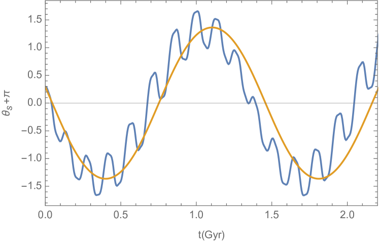
Figure 2: The slow variables $\theta_{\mathrm{s}}+\pi$ (left panel) and $J_{\mathrm{s}}$ (right panel) for the librating orbit of Fig. 1. The blue lines correspond to the numerically integrated orbit, the orange lines to the pendulum approximation.

The blue lines in these plots correspond to the orbit integrated numerically. We see that the motion in $\theta_{\mathrm{s}}$ and $J_{\mathrm{s}}$ is a composition of high frequency, low amplitude oscillations (that are ignored, when invoking the averaging principle), and slow frequency high amplitude oscillations. The pendulum approximation (orange lines), provides a description of the latter.

4 Actions and angles for the pendulum

The action and the angle associated with the pendulum are (e.g., Brizard, 2013), for the case $k<1$,

$$J_{\mathrm{p}}= \frac{4}{\pi}\frac{J_{\mathrm{a}}}{k}\left[\mathrm{E}(k^{2})-(1-k^{2})\mathrm{K}(k^{2})\right],$$ (26)

$$\theta_{\mathrm{p}}= \frac{\pi}{2\mathrm{K}(k^{2})}\mathrm{cn}^{-1}\left(\frac{J_{\mathrm{s}}-J_{\mathrm{s,res}}}{J_{\mathrm{a}}},k^{2}\right).$$

Using $\theta_{\mathrm{p}}$ we can rewrite $\theta_{\mathrm{s}}+g$ as

$$\theta_{\mathrm{s}}+g=2\arcsin\left(k~{}\mathrm{sn}\left(\frac{2}{\pi}\mathrm{K}(k^{2})\theta_{\mathrm{p}},k^{2}\right)\right),$$ (27)

and

$$J_{\mathrm{s}}-J_{\mathrm{s,res}}=J_{\mathrm{a}}~{}\mathrm{cn}\left(\frac{2}{\pi}\mathrm{K}(k^{2})\theta_{\mathrm{p}},k^{2}\right).$$ (28)

For the case $k>1$, one has

$$J_{\mathrm{p}}= \frac{2}{\pi}J_{\mathrm{a}}\mathrm{E}(1/k^{2}),$$ (29)

$$\theta_{\mathrm{p}}= \frac{\pi}{\mathrm{K}(1/k^{2})}\mathrm{dn}^{-1}\left(\frac{J_{\mathrm{s}}-J_{\mathrm{s,res}}}{J_{\mathrm{a}}},1/k^{2}\right).$$

We can rewrite

$$J_{\mathrm{s}}-J_{\mathrm{s,res}}=J_{\mathrm{a}}~{}\mathrm{dn}\left(\frac{\mathrm{K}(1/k^{2})}{\pi}\theta_{\mathrm{p}},1/k^{2}\right).$$ (30)

Figure 3: Contours of conserved quantities associated with the pendulum treatment at the outer Lindblad resonance in the $(-v_{R},v_{\phi})$ plane at $(R,\phi)=(8\,\mathrm{kpc},-25\degr)$ for the bar model presented in this work with $\Omega_{\mathrm{b}}=1.8\Omega_{0}$. The black contours correspond to constant values of $k$ for $k\leq 1$. The thick black contour corresponds to $k=1$. The purple contours correspond to constant values of $k$ for $k>1$. The red dashed contours correspond to constant values of $J_{\mathrm{f}}$. The blue dots correspond to the initial conditions of the orbits shown in Fig. 1.

In Fig. 3, we show $k$ and $J_{\mathrm{f}}$ contours in the velocity space $(-v_{R},v_{\phi})$, for $(R,\phi)=(8\,\mathrm{kpc},-25\degr)$ with the same potential used to integrate the orbits in Fig. 1. The black contours are for $k<1$ (trapped orbits), the green contours for $k>1$ (circulating orbits). The red dashed contours correspond to contours of constant $J_{\mathrm{f}}$. The quantities $k$ (or $J_{\mathrm{p}}$) and $J_{\mathrm{f}}$ characterize an orbit. The blue points correspond to the initial conditions of the two orbits in Fig. 1, which both start from $(R,\phi)=(R_{0},-25\degr)$. The minimum $k=0$ is found at $(-v_{R},v_{\phi})\approx(25,230)\,\mathrm{km}\,\mathrm{s}^{-1}$ and corresponds to the most trapped orbit at the outer Lindblad resonance for such $(R,\phi)$.

5 Averaging distribution functions over pendulum angles

Following the prescription of Binney (2016), we assume that the distribution function for orbits trapped by the resonances ($k<1$) at a certain point $(J_{\mathrm{f}},J_{\mathrm{s}},\theta_{\mathrm{s}})$ is given by the average of the unperturbed DF $f_{0}$ along $\theta_{\mathrm{p}}$, i.e.,

$$f_{\mathrm{tr}}(J_{\mathrm{f}},J_{\mathrm{s}},\theta_{\mathrm{s}})=\frac{1}{2\pi}\int_{0}^{2\pi}f_{0}(J_{\mathrm{f}},J_{\mathrm{s,res}}+\Delta J_{\mathrm{s}}(\theta_{\mathrm{p}}))\mathrm{d}\theta_{\mathrm{p}},$$ (31)

where from Eq. (30)

$$\Delta J_{\mathrm{s}}\equiv J_{\mathrm{a}}~{}\mathrm{cn}\left(\frac{2}{\pi}\mathrm{K}(k^{2})\theta_{\mathrm{p}},k^{2}\right),$$ (32)

and $k$ is a function of $(J_{\mathrm{f}},J_{\mathrm{s}})$, and $\theta_{\mathrm{s}}$, derived from $R$, $\phi$, $v_{R}$, $v_{\phi}$, and the potential. The physical meaning of Eq. (31) is that $f_{\mathrm{tr}}$ corresponds to the unperturbed distribution function $f_{0}$ phase-mixed along the pendulum angle, assuming that enough time elapsed since the growth of the perturbation.

The value of the integral in Eq. (31) depends on the particular form of $f_{0}$. Therefore, in general its solution can be computed numerically as

$$f_{\mathrm{tr}}(J_{\mathrm{f}},J_{\mathrm{s}},\theta_{\mathrm{s}})=\frac{1}{N}\sum_{i}f_{0}(J_{\mathrm{f}},J_{\mathrm{s,res}}+\Delta J_{\mathrm{s}}(\theta_{\mathrm{p}}^{i})),$$ (33)

where $\theta_{\mathrm{p}}^{i}$ sample the orbit between $0$ and $2\pi$, and $N$ is the number of sampling points.

For $k\ll 1$, we can even give an analytic form for the distribution function. To solve this integral, we expand $\ln(f_{0})$ around $J_{\mathrm{s,res}}$ (in typical galaxies $f_{0}$ is almost exponential in $J_{\mathrm{s}}$) as

$$\ln\left(f_{0}(J_{\mathrm{f}},J_{\mathrm{s,res}}+\Delta J_{\mathrm{s}})\right)\approx\ln\left(f_{0}(J_{\mathrm{f}},J_{\mathrm{s,res}})\right)-\frac{\Delta J_{\mathrm{s}}}{J_{\mathrm{h}}},$$ (34)

where

$$J_{\mathrm{h}}\equiv-1\bigg{/}\left(\frac{1}{f_{0}}\frac{\partial f_{0}}{\partial J_{\mathrm{s}}}\right)_{J_{\mathrm{s,res}}}.$$ (35)

Then

$$f_{0}(J_{\mathrm{f}},J_{\mathrm{s,res}}+\Delta J_{\mathrm{s}})\approx f_{0}(J_{\mathrm{f}},J_{\mathrm{s,res}})\mathrm{e}^{-\Delta J_{\mathrm{s}}/J_{\mathrm{h}}}.$$ (36)

This approximation is excellent to express $f_{0}$, but unfortunately, it is not enough to solve the integral from Eq. (31). To do that one more approximation is necessary. Expanding Eq. (32) to first order in $k$, $\Delta J_{\mathrm{s}}$ can be expressed as

$$\Delta J_{\mathrm{s}}\approx J_{\mathrm{a}}\cos{\theta_{\mathrm{p}}},$$ (37)

In this way, de facto, we fall back on the harmonic oscillator solution Eqs. (22)-(23). With these approximations, the solution of the integral from Eq. (31) is

$$f_{\mathrm{tr}}(J_{\mathrm{f}},J_{\mathrm{s}},\theta_{\mathrm{s}})=f_{0}(J_{\mathrm{f}},J_{\mathrm{s,res}})\mathrm{I}_{0}(J_{\mathrm{a}}/J_{\mathrm{h}}),$$ (38)

where $\mathrm{I}_{0}(x)$ is the incomplete Bessel function of the first kind.

For the zone of circulation ($k>1$) we instead use for the distribution function the prescription

$$f_{\mathrm{circ}}(J_{\mathrm{f}},J_{\mathrm{s}},\theta_{\mathrm{s}})=f_{0}(J_{\mathrm{f}},\overline{J_{\mathrm{s}}}),$$ (39)

where

$$\overline{J_{\mathrm{s}}}=\frac{1}{2\pi}\int_{0}^{2\pi}J_{\mathrm{s}}(\theta_{\mathrm{p}})\mathrm{d}\theta_{\mathrm{p}}=J_{\mathrm{s,res}}+\frac{\pi}{2}\frac{J_{\mathrm{a}}}{K(1/k^{2})}.$$ (40)

This prescription is motivated by the fact that, outside of the trapping region, the perturbing potential simply deforms the orbital tori of the underlying axisymmetric system rather than abruptly building completely new tori as it does within the trapping region. Consequently, if the perturbation emerges slowly enough, the phase-space density will be adiabatically constant on each torus as it is deformed at its original value, $f_{0}(\boldsymbol{J})$, where $\boldsymbol{J}=(J_{\mathrm{f}},\overline{J_{\mathrm{s}}})$ is to be understood to be the invariant actions of the perturbed torus rather than momenta of the original system of angle-action variables. Notice that, for large $k$ (far from the resonance), $\overline{J_{\mathrm{s}}}\rightarrow J_{\mathrm{s}}$ rather fast, and we are back to the axisymmetric case (conservation of the angular momentum $J_{\phi}=mJ_{\mathrm{s}}$).

6 Results

We now present a few results of astrophysical interest for the response at the resonances of an unperturbed distribution function $f_{0}$ to the bar perturbation presented in the previous sections.

As an unperturbed distribution function $f_{0}$ we choose (Binney & McMillan, 2011)

$$f_{0}(J_{R},J_{\phi})=\frac{\gamma(R_{\mathrm{g}})\Sigma_{0}\mathrm{e}^{-R_{\mathrm{g}}/h_{R}}}{2\pi\sigma_{R}^{2}(R_{\mathrm{g}})}\mathrm{e}^{-\frac{J_{R}\kappa(R_{\mathrm{g}})}{\sigma_{R}^{2}(R_{\mathrm{g}})}},$$ (41)

where

$$\sigma_{R}(R)=\sigma_{R}(R_{0})\mathrm{e}^{-\frac{R-R_{0}}{5h_{R}}},$$ (42)

with $\gamma$ defined as in Eq. (3), $\sigma_{R}(R_{0})=30\,\mathrm{km}\,\mathrm{s}^{-1}$, and $h_{R}=2\,\mathrm{kpc}$, a reasonable description of the kinematics of the Solar neighbourhood.

Figure 4: Distribution function in the $(-v_{R},v_{\phi})$ plane at different Galactocentric radii $R$ and $\phi=-25\degr$, obtained using the treatment at the resonances and the bar model presented in this work. The bar’s pattern speed is $\Omega_{\mathrm{b}}=1.8.\Omega_{0}$. The thick contours enclose orbits trapped at the outer Lindblad resonance. The distribution function contours enclose (from the outer to the inner) 95, 90, 80, 68, and $50\%$ of the stars.

We first consider, in Fig. 4, the density of stars in local velocity space obtained from a model with a “fast” rotating bar, as in the classical picture (Dehnen, 2000; Antoja et al., 2014; Monari et al., 2017b). For such a bar, the Solar neighbourhood is in the vicinity of the outer Lindblad resonance of the bar. The angle of the bar with respect to the Solar position is taken to be $\phi=-25\degr$. The bar that we present here has $\Omega_{\mathrm{b}}=1.8\Omega_{0}$. We see that, in line with previous studies, the analysis in this work also predicts the formation of a low-velocity overdensity similar to the Hercules moving group (e.g., Dehnen, 1998; Famaey et al., 2005) at positive $v_{R}$, whose velocity position and relative amplitude varies as a function of radius. The group is not formed by orbits trapped by the outer Lindblad resonance, but from circulating orbits with guiding radii inside the $R_{\mathrm{OLR}}$. The orbits trapped to a resonance rather seem to be associated with the feature of local velocity space sometimes called the “horn” (e.g., Monari, 2014). This is also in line with previous studies, but never before had the distribution function in the trapped region been quantified for a fully phase-mixed population. Interestingly, we clearly see that in this case the Hercules moving group shifts both in $v_{\phi}$ (lower $v_{\phi}$ at larger radii) and in $-v_{R}$ (larger $-v_{R}$ at larger radii).

Figure 5: As in Fig. 4, but for a bar’s pattern speed $\Omega_{\mathrm{b}}=1.2\Omega_{0}.$ The thick contours enclose orbits trapped to the corotation.

Recently, Sormani et al. (2015) and Li et al. (2016) have argued that the pattern speed of the bar is $\Omega_{\mathrm{b}}=1.2\Omega_{0}$, significantly lower than in the classical picture. In this case the solar neighbourhood would lie just outside corotation, so in Fig. 5 we also plot the velocity distribution at three such locations. In the central and right panels of Fig. 5, when the zone of trapping is at low azimuthal velocities, a deformation in the velocity distribution at negative $-v_{R}$ that could resemble Hercules forms within the trapping zone rather than outside it. When there is a region of enhanced density below the trapping zone, (left panel of Fig. 5) it occurs at $-v_{R}>0$, as predicted by the Eulerian linear theory, and as such conflicts with the observations. Hence, the pendulum formalism is mandatory if one seeks to explain the Hercules group as a consequence of the corotation resonance, as Pérez-Villegas et al. (2017) did with made-to-measure $N$-body models. Notice that the orbits associated with the overdensity at $(-v_{R},v_{\phi})\approx(-10,210)\,\mathrm{km}\,\mathrm{s}^{-1}$ in the central panel of Fig. 5 are of the same kind of those described by Pérez-Villegas et al. (2017), i.e., trapped around the bar’s Lagrangian points (see Fig. 6).

Figure 6: An orbit trapped to the corotation, integrated in the potential presented in this work with a bar’s pattern speed $\Omega_{\mathrm{b}}=1.2\Omega_{0}$. The orbit is shown in the reference frame corotating with the bar. The initial conditions of this orbit are $(R,\phi)=(8.2\,\mathrm{kpc},-25\degr)$, and $(-v_{R},v_{\phi})=(-10,210)\,\mathrm{km}\,\mathrm{s}^{-1}$. The red dots correspond to the position of the apocentres, and the black thick line to the long axis of the bar. The bar rotates counterclockwise.

Finally we provide the reader with a comparison plot in Fig. 7, in which we display the local velocity distribution obtained from orbits integrated for 6 Gyr in the same potential, after the bar is slowly grown for 3 Gyr with the growth law from Dehnen (2000), and for the same initial $f_{0}$ as in our analytic model (with the backwards integration method of Vauterin & Dejonghe, 1997; Dehnen, 2000).

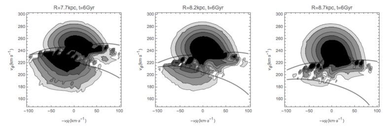
Figure 7: Local velocity distribution obtained from numerically integrating orbits for 6 Gyr after an adiabatic growth of the bar, starting from the same initial $f_{0}$ distribution function as for Fig. 4 and Fig. 5. The resolution of the grid used to obtan this figure is $5\,\mathrm{km}\,\mathrm{s}^{-1}$. Compare the top-row ($\Omega_{\mathrm{b}}=1.8\Omega_{0}$) with Fig. 4, and the bottom row ($\Omega_{\mathrm{b}}=1.2\Omega_{0}$) with Fig. 5.

7 Conclusion

In this paper, we presented for the first time a way to treat an action-based distribution function in the region of action space where orbits are resonantly trapped by a bar, where the Eulerian treatment of Monari et al. (2016a) diverges. The idea is rather to follow the deformation of the tori outside the trapping region, while averaging the distribution function over the relevant angles in the trapping region. We showed that in the trapping region the relevant action-angle variables are those of a pendulum, and averaging over those angles allows for a smooth connection with the deformed tori in the circulation zone. With such distribution functions, we can reproduce an overdensity in velocity space resembling the Hercules moving group both outside the outer Lindblad resonance and outside corotation of a bar. The linearized Eulerian treatment of Monari et al. (2017a) is unable to handle the latter possibility. The disturbances in velocity space that are caused by the inner Lindblad and corotation resonances move in different ways through velocity space as one changes location within the disc (Figs 4 and 5). Consequently, it will be straightforward to determine which resonance is responsible for the Hercules group, once we can reliably map velocity space in many locations.

This formalism opens the way to fitting quantitatively the effects of the bar in an action-based modelling of the Milky Way. Nevertheless, there remain multiple tests to be done, which are beyond the scope of the present contribution presenting the relevant formalism. In particular, the prediction of a fully phase-mixed distribution function in the trapping region should be compared to the outcome of various simulations, to check over which time-scales phase-mixing is efficient enough to reproduce our results. Moreover, the process of trapping and the associated filling of the region of resonant trapping in action space is not necessarily going to be based purely on the phase-mixing of the original axisymmetric distribution function, especially if the growth of the bar is rapid. But even in this case, the advantage of the present paper has been to present the relevant pendulum action variables on which to base a parametric distribution function to fit both simulations and real data in the trapping zone.

As a matter of fact, only the upcoming Gaia data will allow us to check whether our phase-mixing of the original distribution function is actually a good representation of the Galactic disc at different radii. If not, knowing that our distribution function must depend only on the new set of action variables within the trapping region, we will be able to leave its functional form free, and fit it to the data. This approach is very fast and does not require to perform numerous expensive simulations. As a consequence, one will be able to explore very efficiently the parameter space of the perturbations.

Further improvements of the present formalism will need taking into account the vertical $z$ direction, the time dependence in the amplitude of perturbations, as well as collective effects (e.g., Weinberg, 1989; Fouvry et al., 2015b). It will also be mandatory to move away from the epicyclic approximation (McGill & Binney, 1990; Sanders & Binney, 2015). Once this will be done, in the absence of strong resonance overlaps, a complete dynamical model of the present-day Milky Way disc could then in principle finally be built by applying, on top of the trapped distribution function near the main resonances of each perturber, our previous Eulerian treatment of perturbations (Monari et al., 2016a) for the other perturbers, even including vertical perturbations and “bending” modes of the disc (Widrow et al., 2014; Xu et al., 2015; Laporte et al., 2016).

Appendix A Jacobi special functions

The Jacobi $\mathrm{sn}$, $\mathrm{cn}$, and $\mathrm{dn}$ functions can be evaluated as the sum of a power series, and are defined as

$$\mathrm{sn}(u,m)\equiv\sin(\varphi),\quad\mathrm{cn}(u,m)\equiv\cos(\varphi),$$ (43)

with

$$u=\int_{0}^{\varphi}\frac{\mathrm{d}\theta}{\sqrt{1-m\sin^{2}\theta}}.$$ (44)

The $\mathrm{dn}$ function is defined as

$$\mathrm{dn}(u,m)^{2}\equiv 1-m~{}\mathrm{sn}^{2}(u,m).$$ (45)

The elliptic functions $\mathrm{E}$ and $\mathrm{K}$ are defined as

$$\mathrm{E}(m)=\int_{0}^{\pi/2}\mathrm{d}\theta{\sqrt{1-m\sin^{2}\theta}},$$ (46)

$$\mathrm{K}(m)=\int_{0}^{\pi/2}\frac{\mathrm{d}\theta}{\sqrt{1-m\sin^{2}\theta}}.$$ (47)

References

- Antoja et al. (2014) Antoja T. et al., 2014, A&A, 563, A60
- Arnold (1978) Arnold V. I., 1978, Mathematical methods of classical mechanics. Springer, New York
- Aumer & Binney (2017) Aumer M., Binney J., 2017, arXiv:1705.09240
- Aumer et al. (2016) Aumer M., Binney J., Schönrich R., 2016, MNRAS, 462, 1697
- Binney (2016) Binney J., 2016, MNRAS, 462, 2792
- Binney et al. (1997) Binney J., Gerhard O., Spergel D., 1997, MNRAS, 288, 365
- Binney et al. (1991) Binney J., Gerhard O. E., Stark A. A., Bally J., Uchida K. I., 1991, MNRAS, 252, 210
- Binney & McMillan (2011) Binney J., McMillan P., 2011, MNRAS, 413, 1889
- Binney & Piffl (2015) Binney J., Piffl T., 2015, MNRAS, 454, 3653
- Binney & Tremaine (2008) Binney J., Tremaine S., 2008, Galactic Dynamics: Second Edition. Princeton University Press
- Bovy et al. (2015) Bovy J., Bird J. C., García Pérez A. E., Majewski S. R., Nidever D. L., Zasowski G., 2015, ApJ, 800, 83
- Brizard (2013) Brizard A. J., 2013, Communications in Nonlinear Science and Numerical Simulation, 18, 511
- Chirikov (1979) Chirikov B. V., 1979, Phys. Rep., 52, 263
- Cole & Binney (2017) Cole D. R., Binney J., 2017, MNRAS, 465, 798
- de Vaucouleurs (1964) de Vaucouleurs G., 1964, in IAU Symposium, Vol. 20, The Galaxy and the Magellanic Clouds, Kerr F. J., ed., p. 195
- Dehnen (1998) Dehnen W., 1998, AJ, 115, 2384
- Dehnen (1999) Dehnen W., 1999, AJ, 118, 1190
- Dehnen (2000) Dehnen W., 2000, AJ, 119, 800
- Famaey et al. (2005) Famaey B., Jorissen A., Luri X., Mayor M., Udry S., Dejonghe H., Turon C., 2005, A&A, 430, 165
- Fouvry et al. (2015a) Fouvry J.-B., Binney J., Pichon C., 2015a, ApJ, 806, 117
- Fouvry et al. (2015b) Fouvry J. B., Pichon C., Magorrian J., Chavanis P. H., 2015b, A&A, 584, A129
- Fouvry et al. (2015c) Fouvry J.-B., Pichon C., Prunet S., 2015c, MNRAS, 449, 1967
- Gaia Collaboration et al. (2016) Gaia Collaboration et al., 2016, A&A, 595, A1
- Grand et al. (2015) Grand R. J. J., Bovy J., Kawata D., Hunt J. A. S., Famaey B., Siebert A., Monari G., Cropper M., 2015, MNRAS, 453, 1867
- Kaasalainen (1994) Kaasalainen M., 1994, MNRAS, 268, 1041
- Laporte et al. (2016) Laporte C. F. P., Gómez F. A., Besla G., Johnston K. V., Garavito-Camargo N., 2016, arXiv:1608.04743
- Lawden (1989) Lawden D., 1989, Elliptic Functions and Applications, Applied mathematical sciences. Springer
- Li et al. (2016) Li Z., Gerhard O., Shen J., Portail M., Wegg C., 2016, ApJ, 824, 13
- McGill & Binney (1990) McGill C., Binney J., 1990, MNRAS, 244, 634
- McMillan (2013) McMillan P. J., 2013, MNRAS, 430, 3276
- Monari (2014) Monari G., 2014, PhD thesis, Rijksuniversiteit Groningen
- Monari et al. (2015) Monari G., Famaey B., Siebert A., 2015, MNRAS, 452, 747
- Monari et al. (2016a) Monari G., Famaey B., Siebert A., 2016a, MNRAS, 457, 2569
- Monari et al. (2017a) Monari G., Famaey B., Siebert A., Duchateau A., Lorscheider T., Bienaymé O., 2017a, MNRAS, 465, 1443
- Monari et al. (2016b) Monari G., Famaey B., Siebert A., Grand R. J. J., Kawata D., Boily C., 2016b, MNRAS, 461, 3835
- Monari et al. (2017b) Monari G., Kawata D., Hunt J. A. S., Famaey B., 2017b, MNRAS, 466, L113
- Pérez-Villegas et al. (2017) Pérez-Villegas A., Portail M., Wegg C., Gerhard O., 2017, ApJ, 840, L2
- Sanders & Binney (2015) Sanders J. L., Binney J., 2015, MNRAS, 447, 2479
- Sellwood & Carlberg (2014) Sellwood J. A., Carlberg R. G., 2014, ApJ, 785, 137
- Sormani et al. (2015) Sormani M. C., Binney J., Magorrian J., 2015, MNRAS, 454, 1818
- Trick et al. (2017) Trick W. H., Bovy J., D’Onghia E., Rix H.-W., 2017, ApJ, 839, 61
- Vauterin & Dejonghe (1997) Vauterin P., Dejonghe H., 1997, MNRAS, 286, 812
- Wegg et al. (2015) Wegg C., Gerhard O., Portail M., 2015, MNRAS, 450, 4050
- Weinberg (1989) Weinberg M. D., 1989, MNRAS, 239, 549
- Weinberg (1994) Weinberg M. D., 1994, ApJ, 420, 597
- Widrow et al. (2014) Widrow L. M., Barber J., Chequers M. H., Cheng E., 2014, MNRAS, 440, 1971
- Williams et al. (2013) Williams M. E. K. et al., 2013, MNRAS, 436, 101
- Xu et al. (2015) Xu Y., Newberg H. J., Carlin J. L., Liu C., Deng L., Li J., Schönrich R., Yanny B., 2015, ApJ, 801, 105