Ticker: A System for Incremental ASP-based Stream Reasoning

Abstract

In complex reasoning tasks, as expressible by Answer Set Programming (ASP), problems often permit for multiple solutions. In dynamic environments, where knowledge is continuously changing, the question arises how a given model can be incrementally adjusted relative to new and outdated information. This paper introduces Ticker, a prototypical engine for well-defined logical reasoning over streaming data. Ticker builds on a practical fragment of the recent rule-based language LARS which extends Answer Set Programming for streams by providing flexible expiration control and temporal modalities. We discuss Ticker’s reasoning strategies: First, the repeated one-shot solving mode calls Clingo on an ASP encoding. We show how this translation can be incrementally updated when new data is streaming in or time passes by. Based on this, we build on Doyle’s classic justification-based truth maintenance system (TMS) to update models of non-stratified programs. Finally, we empirically compare the obtained evaluation mechanisms. This paper is under consideration for acceptance in TPLP.

1 Introduction

Stream reasoning [Della Valle et al. (2009)] as research field emerged from data processing [Babu and Widom (2001)], i.e., the handling of continuous queries in a frequently changing database. Work in Knowledge Representation & Reasoning, e.g. [Ren and Pan (2011), Gebser et al. (2015)], shifts the focus from high throughput to high expressiveness of declarative queries and programs. In particular, the logic-based framework LARS [Beck et al. (2015)] was defined as an extension of Answer Set Programming (ASP) with window operators for deliberately dropping data, e.g., based on time or counting atoms, and controlling the temporal modality in the resulting windows.

When dealing with complex reasoning tasks in stream settings, one may in general not afford to recompute models from scratch every time new data comes in or when older portions of data become outdated. Besides the pragmatic need for efficient computation, there is also a semantic issue: while aspects of a solution might have to change dynamically and potentially quickly, typically not everything should be reconstructed from scratch, but adapted to fit the current data.

Recently, many stream processing tools and reasoning features have been proposed, e.g. [Barbieri et al. (2010), Phuoc et al. (2011), Gebser et al. (2014)]. However, an ASP-based stream reasoning engine that supports window operators and has an incremental model update mechanism is lacking to date. This may be explained by the fact that nonmonotonic negation, beyond recursion, makes efficient incremental update non-trivial; combined with temporal reasoning modalities over data windows, this becomes even more challenging.

Contributions. We tackle this issue and make the following contributions.

• We present a notion of tick streams to formally represent the sequential steps of a fully incremental stream reasoning system.

• Based on this, we give an intuitive translation of a practical fragment of LARS programs, plain LARS, to ASP suitable for standard one-shot solving, and in particular, stratified programs.

• Next, we develop an ASP encoding that can be incrementally updated when time passes by or when new input arrives.

• We then present Ticker, our prototype reasoning engine that comes with two reasoning strategies. One utilizes Clingo [Gebser et al. (2014)] with a static ASP encoding, the other truth maintenance techniques [Doyle (1979)] to adjust models based on the incremental encoding.

• Finally, we experimentally compare the two reasoning modes in application scenarios. The results demonstrate the performance benefits that arise from incremental evaluation.

In summary, we provide a novel technique for adjusting an ASP-based stream reasoning program by time and data streaming in. In particular, the update technique of the program is independent of the model update technique used to process the program change.

2 Stream Reasoning in LARS

We will gradually introduce the central concepts of LARS [Beck et al. (2015)] tailored to the considered fragment. If appropriate, we give only informal descriptions.

Throughout, we distinguish extensional atoms $A^{E}$ for input data and intensional atoms $A^{I}$ for derived information. By $A=A^{E}\cup A^{I}$, we denote the set of atoms.

Definition 1 (Stream).

A stream ${S=(T,\upsilon)}$ consists of a timeline $T$, which is a closed nonempty interval in $\mathbb{N}$, and an evaluation function ${\upsilon:\mathbb{N}\mapsto 2^{A}}$. The elements ${t\in T}$ are called time points.

Intuitively, a stream $S$ associates with each time point a set of atoms. We call $S$ a data stream, if it contains only extensional atoms. To cope with the amount of data, one usually considers only recent atoms. Let ${S=(T,\upsilon)}$ and ${S^{\prime}=(T^{\prime},\upsilon^{\prime})}$ be two streams such that ${S^{\prime}\subseteq S}$, i.e., ${T^{\prime}\subseteq T}$ and ${\upsilon^{\prime}(t^{\prime})\subseteq\upsilon(t^{\prime})}$ for all ${t^{\prime}\in T^{\prime}}$. Then $S^{\prime}$ is called a window of $S$.

Definition 2 (Window function).

Any (computable) function $w$ that returns, given a stream $S=(T,\upsilon)$ and a time point ${t\in\mathbb{N}}$, a window $S^{\prime}$ of $S$, is called a window function.

Widely used are time-based window functions, which select all atoms appearing in last $n$ time points, and tuple-based window functions, which select a fixed number of latest tuples. To this end, we define the tuple size $|S|$ of a stream $S=(T,\upsilon)$ as $|\{(a,t)\mid t\in T,a\in\upsilon(t)\}|$.

Definition 3 (Sliding Time-based and Tuple-based Window).

Let ${S=(T,\upsilon)}$ be a stream, $t\in T=[t_{1},t_{m}]$ and let ${n\in\mathbb{N}\cup\{\infty\}}$. Then,

• the sliding time-based window function $\tau_{n}$ (for size $n$) is ${\tau_{n}(S,t)=(T^{\prime},\upsilon|_{T^{\prime}})}$, where ${T^{\prime}=[t^{\prime},t]}$ and ${t^{\prime}=\max\{t_{1},t-n\}}$;

• the sliding tuple-based window function $\#_{n}$ (for size $n$) is

  $$\#_{n}(S,t)=\begin{cases}\tau_{t-t^{\prime}}(S,t)&\text{if}~{}|\tau_{t-t^{\prime}}(S,t)|\leq n,\\ S^{\prime}&\text{else,}\end{cases}$$

  where $t^{\prime}=\max(\{u\in T\mid|\tau_{t-u}(S,t)|\geq n\}\cup\{t_{1}\})$ and $S^{\prime}=([t^{\prime},t],\upsilon^{\prime})$ has tuple size $|S^{\prime}|=n$ such that $\upsilon^{\prime}(u)=\upsilon(u)$ for all $u\in[t^{\prime}+1,t]$ and $\upsilon^{\prime}(t^{\prime})\subseteq\upsilon(t^{\prime})$.

Note that in general, multiple options exist for defining $\upsilon^{\prime}$ at $t^{\prime}$ in the tuple-based window. However, we assume a deterministic choice as specified by the implementation of the function. In particular, we will later consider that atoms are streaming in an order, which leads to a natural, unique cut-off position based on counting.

Example 1.

Fig. 1 window depicts at partial stream $S=([35,41],\upsilon)$, where $\upsilon=\{35\mapsto\{a(x)\},$ $37\mapsto\{a(y),a(z)\},39\mapsto\{a(x)\}\}$, and a time window of length $3$ at time $t=40$, which corresponds to a tuple window of size $3$ there. Notably, there are two options for a tuple window of size $2$, both of which select timeline $[37,40]$, but only one of the atoms at time $37$, respectively.  $\mathbin{\scalebox{0.6}{$\blacksquare$}}$

We also use window functions with streams as single argument, applied implicitly at the end of the timeline, i.e., if $S=([t_{0},t],\upsilon)$, then $\tau_{n}(S)$ abbreviates $\tau_{n}(S,t)$ and $\#_{n}(S)$ stands for $\#_{n}(S,t)$.

Figure 1: Temporal extent of a sliding tuple-based window of size 3 (or 2) at $t=40$

Window operators $\boxplus^{w}$. A window function $w$ can be accessed in rules by window operators. That is to say, an expression $\boxplus^{w}\alpha$ has the effect that $\alpha$ is evaluated on the “snapshot” of the data stream delivered by its associated window function $w$. Within the selected snapshot, LARS allows for controlling the temporal semantics with further modalities.

Temporal modalities. Let ${S=(T,\upsilon)}$ be a stream, ${a\in A}$ and ${\mathrm{B}\subseteq A}$ static background data. Then, at time point ${t\in T}$,

• $a$ holds, if ${a\in\upsilon(t)}$ or ${a\in\mathrm{B}}$;

• $\Diamond a$ holds, if $a$ holds at some time point ${t^{\prime}\in T}$;

• $\Box a$ holds, if $a$ holds at all time points ${t^{\prime}\in T}$; and

• $@_{t^{\prime}}a$ holds, where $t^{\prime}\in\mathbb{N}$, if $t^{\prime}\in T$ and $a$ holds at $t^{\prime}$.

The set $A^{+}$ of extended atoms $e$ is given by the grammar $e\;::=\;a\mid@_{t}a\mid\boxplus^{w}@_{t}a\mid\boxplus^{w}\Diamond a\mid\boxplus^{w}\Box a\,,$ where $a\in A$ and $t$ is any time point. The expressions $@_{t}a$ are called $@$-atoms; ${\boxplus^{w}\mathbin{\star}a}$, where ${\mathbin{\star}\in\{@_{t},\Diamond,\Box\}}$, are window atoms. We write $\boxplus^{n}$ for $\boxplus^{\tau_{n}}$, which is not to be confused with $\boxplus^{\#n}$.

Example 2 (cont’d).

At $t=40$, $\boxplus^{3}\Diamond a(x)$ and $\boxplus^{3}@_{37}a(y)$ hold, as does $\boxplus^{\#1}\Box a(x)$ at $t=35,39$.  $\mathbin{\scalebox{0.6}{$\blacksquare$}}$

2.1 Plain LARS Programs

We use a fragment of the formalism in [Beck et al. (2015)], called plain LARS programs.

Syntax. A (ground plain LARS) program $P$ is a set of rules of the form

$$\alpha\leftarrow\beta_{1},\dots,\beta_{j},\operatorname{not}\beta_{j+1},\dots,\operatorname{not}\beta_{n}\,,$$ (1)

where the head $\alpha$ is of form $a$ or $@_{t}a$, ${a\in A^{I}}$, and in the body $\beta(r)=\beta_{1},\dots,\beta_{j},\operatorname{not}\beta_{j+1},\dots,\operatorname{not}\beta_{n}$ each $\beta_{i}$ is an extended atom. We let $H(r)=\alpha$ and $\mathit{B}(r)=\mathit{B}^{+}(r)\cup\mathit{B}^{-}(r)$, where $\mathit{B}^{+}(r)=\{\beta_{1},$ $\ldots,$ $\beta_{j}\}$ and $\mathit{B}^{-}(r)=\{\beta_{j+1},\ldots,\beta_{n}\}$ are the the positive, resp. negative body atoms of $r$.

Semantics. For a data stream ${D=(T_{D},\upsilon_{D})}$, any stream ${I=(T,\upsilon)\supseteq D}$ that coincides with $D$ on $A^{E}$, i.e., $a{\,\in\,}\upsilon(t)\cap A^{E}$ iff $a{\,\in\,}\upsilon_{D}(t)$, is an interpretation stream for $D$. A tuple ${M=\langle I,W,\mathrm{B}\rangle}$, where $W$ is a set of window functions and $\mathrm{B}$ is the background knowledge, is then an interpretation for $D$. Throughout, we assume $W=\{\tau_{k},\#_{n}\mid k,n\in\mathbb{N}\}$ and $\mathrm{B}$ are fixed and also omit them.

Satisfaction by $M$ at ${t\in T}$ is as follows: ${M,t\models\alpha}$ for ${\alpha\in A^{+}}$, if $\alpha$ holds in ${(T,\upsilon)}$ at time ${t}$; ${M,t\models r}$ for rule $r$, if ${M,t\models\beta(r)}$ implies ${M,t\models H(r)}$, where ${M,t\models\beta(r)}$, if (i) ${M,t\models\beta_{i}}$for all ${i\in\{1,\dots,j\}}$ and (ii) ${M,t\not\models\beta_{i}}$for all ${i\in\{j{+}1,\dots,n\}}$; and ${M,t\models P}$ for program $P$, i.e., $M$ is a model of $P$ (for $D$) at ${t}$, if ${M,t\models r}$ for all ${r\in P}$. Moreover, ${M}$ is minimal, if in addition no model ${M^{\prime}=\langle S^{\prime},W,\mathrm{B}\rangle\neq M}$ of $P$ exists such that $S^{\prime}=(T,\upsilon^{\prime})$ and ${\upsilon^{\prime}\subseteq\upsilon}$.

Definition 4 (Answer Stream).

An interpretation stream $I$ is an answer stream of program $P$ for the data stream ${D\subseteq I}$ at time $t$, if ${M=\langle I,W,\mathrm{B}\rangle}$ is a minimal model of the reduct $P^{M,t}=\{r\in P\mid M,t\models\beta(r)\}$. By $AS(P,D,t)$ we denote the set of all such answer streams $I$.

Example 3 (cont’d).

Consider $D$ from Fig. 1 and $P=\{b(x)\leftarrow\boxplus^{3}\Diamond a(x)\}$. Then, for all $t\in[35,41]$ the answer stream $I$ at $t$ is unique and adds to $D$ the mapping $t\mapsto\{b(x)\}$. $\mathbin{\scalebox{0.6}{$\blacksquare$}}$

Non-ground programs. The semantics for LARS is formally defined for ground programs but extends naturally for the non-ground case by considering the respective ground instantiations.

Windows on intensional/extensional atoms. For practical reasons, we consider tuple windows only on extensional data. Their intended use is counting input data, not inferences; using them on intensional data is conceptually questionable.

Example 4.

Consider the rule $r=b\leftarrow\boxplus^{\#1}\Diamond a$ and the stream $S=([0,1],\{0\mapsto\{a\}\})$, which is not a model for $r$, since the rule fires and we thus must have $b$ at time $1$. However, in this interpretation, $\boxplus^{\#1}\Diamond a$ does not hold any more, if we also take into account the inference $b$. Thus, the interpretation would not be minimal. Moreover, further inferences would not be founded. Hence, program $\{r\}$ has no model. $\mathbin{\scalebox{0.6}{$\blacksquare$}}$

In contrast to tuple windows, time windows are useful and allowed on arbitrary data, as long as no cyclic positive dependencies through time-based window atoms $\boxplus^{n}\Box a$ occur.

Example 5.

Assume a range of values $V=0,\dots,30$, among which $V\geq 18$ are considered ‘high.’ To test whether the predicate $\mathit{alpha}$ always had a high value during the last $n$ time points, we first abstract by $@_{T}\mathit{high}\leftarrow\boxplus^{n}@_{T}\mathit{alpha}(V),V\geq 18$ for and then test $\mathit{yes}\leftarrow\boxplus^{n}\Box\mathit{high}$.  $\mathbin{\scalebox{0.6}{$\blacksquare$}}$

3 Static ASP Encoding

In this section we will first give a translation of LARS programs $P$ to an ASP program $\hat{P}$. Toward incremental evaluation of $P$, we will then show how $\hat{P}$ can be adjusted to accommodate new input signals and account for expiring information as specified by window operators.

Definition 5 (Tick).

A pair $k=(t,c)$, where $t,c\in\mathbb{N}$, is called a tick, with $t$ the (tick) time and $c$ the (tick) count; $(t+1,c)$ is called the time increment and $(t,c+1)$ the count increment of $k$. A sequence $K=\langle k_{1},\dots,k_{m}\rangle$, $m\geq 1$, of ticks is a tick pattern, if every tick $k_{i+1}$ is either a time increment or a count increment of $k_{i}$.

Intuitively, a tick pattern captures the incremental development of a stream in terms of time and tuple count, where at each step exactly one dimension increases by 1. For a set of ticks, at most one linear ordering yields a tick pattern. Thus, we can view a tick pattern $K$ also as set.

Definition 6 (Tick Stream).

A tick stream is a pair $\dot{S}=(K,v)$ of a tick pattern $K$ and an evaluation function $v$ s.t. $v(k_{i+1})=\{a\}$ for some $a\in A$, if $k_{i+1}$ is a count increment of $k_{i}$, else $v(k_{i+1})=\emptyset$.

We say that a tick stream ${\dot{S}=(K,v)}$ with $K=\langle(t_{1},c_{1}),\dots,(t_{m},c_{m})\rangle$ is at tick $(t_{m},c_{m})$. By default, we assume $(t_{1},c_{1})=(0,0)$ and thus $c_{m}$ is the total number of atoms. We also write $v(t,c)$ instead of $v((t,c))$. Naturally, a (tick) substream $\dot{S}^{\prime}\subseteq\dot{S}$ is a tick stream $(K^{\prime},v^{\prime})$, where $K^{\prime}$ is a subsequence of $K$ and $v^{\prime}$ is the restriction $v|_{K^{\prime}}$ of $v$ to $K^{\prime}$, i.e., $v^{\prime}(t,c)=v(t,c)$ if $(t,c)\in K^{\prime}$, else $v^{\prime}(t,c)=\emptyset$.

Example 6.

The sequence $K=\langle(0,0),(1,0),(2,0),(3,0),(3,1),(3,2),(4,2)\rangle$ is a “canonical” tick pattern starting at $(0,0)$, where $(3,1)$ and $(3,2)$ are the only count increments. Employing an evaluation $v(3,1)=\{a\}$ and $v(3,2)=\{b\}$, we get a tick stream $\dot{S}=(K,v)$ which is at tick $(4,2)$. $\mathbin{\scalebox{0.6}{$\blacksquare$}}$

Definition 7 (Ordering).

Let $\dot{S}=(K,v)$ be a tick stream, where $K=\langle(t_{1},c_{1}),\dots,(t_{m},c_{m})\rangle$, and let $S=(T,\upsilon)$ be a stream such that $T=[t_{1},t_{m}]$ and $\upsilon(t)=\bigcup\{v(t,c)\mid(t,c)\in K\}$ for all $t\in T$. Then, we say $\dot{S}$ is an ordering of $S$, and $S$ underlies $\dot{S}$.

Note that in general, a stream $S$ has multiple orderings, but every tick stream $\dot{S}$ has a unique underlying stream. All orderings of a stream have the same tick pattern.

Example 7 (cont’d).

Stream $S=([0,4],\upsilon)$, where $\upsilon=\{3\mapsto\{a,b\}\}$, is the underlying stream of $\dot{S}$ of Ex. 6. A further ordering of $S$ is $\dot{S}^{\prime}=(K,v^{\prime})$, where $v^{\prime}=\{(3,1)\mapsto\{b\},(3,2)\mapsto\{a\}\}$.  $\mathbin{\scalebox{0.6}{$\blacksquare$}}$

Sliding windows as in Def. 3 carry over naturally for tick streams. There are two central differences. First, ticks replace time points as positions in a stream, and thus as second argument of the window functions. Second, tuple-based windows are now always unique.

Definition 8 (Sliding Windows over Tick Streams).

Let $\dot{S}=(K,v)$ be a tick stream, where $K=\langle(t_{1},c_{1}),\dots,(t_{m},c_{m})\rangle$ and $(t,c)\in K$. Then the time window function $\tau_{n}$, $n\geq 0$, is defined by $\tau_{n}(\dot{S},(t,c))=(K^{\prime},v|_{K^{\prime}})$, where $K^{\prime}=\{(t^{\prime},c^{\prime})\in K\mid\max\{t_{1},t-n\}\leq t^{\prime}\leq t\}$, and the tuple window function $\#_{n}$, $n\geq 1$, by $\#_{n}(\dot{S},(t,c)){=}(K^{\prime},v|_{K^{\prime}})$, where $K^{\prime}{=}\{(t^{\prime},c^{\prime})\in K{\,\mid}\max\{c_{1},c-n+1\}{\,\leq\,}c^{\prime}{\,\leq\,}c\}$.

As for Def. 3, we consider windows over tick streams also implicitly at the end of the timeline.

Lemma 1.

If stream $S$ underlies tick stream $\dot{S}$, then $\tau_{n}(S)$ underlies $\tau_{n}(\dot{S})$.

Example 8 (cont’d).

Given $\dot{S}$ and $S$ from Example 7, we have $\tau_{1}(\dot{S},4)=(\langle(3,0),(3,1),(3,2),$ $(4,2)\rangle,v)$ with underlying stream $\tau_{1}(S,4)=([3,4],\upsilon)$. $\mathbin{\scalebox{0.6}{$\blacksquare$}}$

Correspondence for tuple windows is more subtle due to the different options to realize them.

Lemma 2.

Let stream $S$ underlie tick stream $\dot{S}$ and assume the tuple window $\#_{n}(S)$ is based on the order in which atoms appeared in $S$. Then, $\#_{n}(S)$ underlies $\#_{n}(\dot{S})$.

Example 9 (cont’d).

Stream $S$ has two tuple windows of size $1$: $S_{a}=([3,4],\{3\mapsto\{a\}\})$ and $S_{b}=([3,4],\{3\mapsto\{b\}\})$; the latter underlies $\#_{1}(\dot{S})=(\langle(3,2),(4,2)\rangle,(3,2)\mapsto\{b\})$.  $\mathbin{\scalebox{0.6}{$\blacksquare$}}$

We can represent a stream $S=(T,\upsilon)$ alternatively by $T$ and a set of time-pinned atoms, i.e., the set $\{a_{@}({\mathbf{x}},t)\mid a({\mathbf{x}})\in\upsilon(t),t\in T\}$. Similarly, tick streams can be modelled by tick-pinned atoms of form $a_{\#}({\mathbf{x}},t,c)$, where $c$ increases by 1 for every incoming signal.

Example 10 (cont’d).

Given extra knowledge about the time $t=4$, stream $S$ is fully represented by $\{a_{@}(3),b_{@}(3)\}$, whereas tick stream $\dot{S}$ can be encoded by the set $\{a_{\#}(3,1),b_{\#}(3,2)\}$. $\mathbin{\scalebox{0.6}{$\blacksquare$}}$

The notions of data/interpretation stream readily carry over to their tick analogues. Moreover, we say a tick interpretation stream $I$ is an answer stream of program $P$ (for tick data stream $D$ at $t$), if the underlying stream $I^{\prime}$ of $I$ is an answer stream of $P$ (for the underlying data stream $D^{\prime}$ at $t$).

1

Input: A (potentially non-ground) plain LARS program $P$, and the evaluation time point $t$

2

Output: ASP encoding $\hat{P}$, i.e., a set of normal logic rules

3

4

5$Q~{}\mathtt{:=}~{}\{\,a({\mathbf{X}})\leftarrow\mathit{now}(\dot{N}),a_{@}({\mathbf{X}},\dot{N});\;a_{@}({\mathbf{X}},\dot{N})\leftarrow\mathit{now}(\dot{N}),a({\mathbf{X}})\mid a\text{ is a predicate in }P\}$

6 $R~{}\mathtt{:=}~{}\bigcup_{r\in P}\mathit{larsToAspRules}(r)$

7 return $Q\cup R\cup\{\mathit{now(t)}\}$

8 

9defn $\mathit{larsToAspRules}(r)$ $=$ $\{\mathit{baseRule}(r)\}\cup\,\bigcup_{i=1}^{m}\mathit{windowRules}(e_{i})$

10

11

12defn $\mathit{baseRule}(h\leftarrow e_{1},\dots,e_{n},\operatorname{not}e_{n+1},\dots,\operatorname{not}e_{m})$ $=$

13       $\mathit{atm}(h)\leftarrow\mathit{atm}(e_{1}),\dots,\mathit{atm}(e_{n}),\operatorname{not}\,\mathit{atm}(e_{n+1}),\dots,\operatorname{not}\,\mathit{atm}(e_{m})$

14

15

16defn $\mathit{atm}(e)=\textnormal{{match}}~{}e$

17       case  $a({\mathbf{X}})\textnormal{{$\;\;\Rightarrow\;\;$}}a({\mathbf{X}})$

18       case  $@_{T}a({\mathbf{X}})\textnormal{{$\;\;\Rightarrow\;\;$}}a_{@}({\mathbf{X}},T)$

19       case  $\boxplus^{w}@_{T}a({\mathbf{X}})\textnormal{{$\;\;\Rightarrow\;\;$}}\omega_{e}({\mathbf{X}},T)$ // $\omega_{e}$ is a fresh predicate associated with $e$

20       case  $\boxplus^{w}\Diamond a({\mathbf{X}})\textnormal{{$\;\;\Rightarrow\;\;$}}\omega_{e}({\mathbf{X}})$

21       case  $\boxplus^{w}\Box a({\mathbf{X}})\textnormal{{$\;\;\Rightarrow\;\;$}}\omega_{e}({\mathbf{X}})$

22      

23

24

25defn $\mathit{windowRules}(e)=\textnormal{{match}}~{}e$

26       case  $\boxplus^{n}@_{T}a({\mathbf{X}})\textnormal{{$\;\;\Rightarrow\;\;$}}\{\,\omega_{e}({\mathbf{X}},T)\leftarrow\mathit{now}(\dot{N}),a_{@}({\mathbf{X}},T),T=\dot{N}-i\mid i=0,\dots,n\,\}$

27       case  $\boxplus^{n}\Diamond a({\mathbf{X}})\textnormal{{$\;\;\Rightarrow\;\;$}}\{\,\omega_{e}({\mathbf{X}})\leftarrow\mathit{now}(\dot{N}),a_{@}({\mathbf{X}},T),T=\dot{N}-i\mid i=0,\dots,n\,\}$

28       case  $\boxplus^{n}\Box a({\mathbf{X}})\textnormal{{$\;\;\Rightarrow\;\;$}}\{\,\omega_{e}({\mathbf{X}})\leftarrow a({\mathbf{X}}),\operatorname{not}\,\mathit{spoil}_{e}({\mathbf{X}})\,\}\,\cup$

29        $\{\,\mathit{spoil}_{e}({\mathbf{X}})\leftarrow a({\mathbf{X}}),\mathit{now}(\dot{N}),\operatorname{not}\,a_{@}({\mathbf{X}},T),T=\dot{N}-i\mid i=1,\dots,n\,\}$

30       case  $\boxplus^{\#n}@_{T}a({\mathbf{X}})\textnormal{{$\;\;\Rightarrow\;\;$}}\{\,\omega_{e}({\mathbf{X}},T)\leftarrow\mathit{cnt}(\dot{C}),a_{\#}({\mathbf{X}},T,D),D=\dot{C}-j\mid j=0,\dots,n-1\,\}$

31       case  $\boxplus^{\#n}\Diamond a({\mathbf{X}})\textnormal{{$\;\;\Rightarrow\;\;$}}\{\,\omega_{e}({\mathbf{X}})\leftarrow\mathit{cnt}(\dot{C}),a_{\#}({\mathbf{X}},T,D),D=\dot{C}-j\mid j=0,\dots,n-1\,\}$

32       case  $\boxplus^{\#n}\Box a({\mathbf{X}})\textnormal{{$\;\;\Rightarrow\;\;$}}\{\,\omega_{e}({\mathbf{X}})\leftarrow a({\mathbf{X}}),\operatorname{not}\,\mathit{spoil}_{e}({\mathbf{X}})\,\}\,\cup$

33        $\{\,\mathit{spoil}_{e}({\mathbf{X}})\leftarrow a({\mathbf{X}}),\mathit{cnt}(\dot{C}),\mathit{tick}(T,D),\dot{C}-n+1\leq D\leq\dot{C},\,\operatorname{not}\,a_{@}({\mathbf{X}},T)\,\}\,\cup$

34        $\{\,\mathit{spoil}_{e}({\mathbf{X}})\leftarrow a({\mathbf{X}}),\mathit{cnt}(\dot{C}),\mathit{tick}(T,D),D=\dot{C}-n+1,\,a_{\#}({\mathbf{X}},T,D^{\prime}),\,D^{\prime}<D\,\}$

35       else $~{}\emptyset$

36      

37

Algorithm 1 Plain LARS Program to ASP $\mathit{LarsToAsp}(P,t)$

LARS to ASP (Algorithm 1). Plain LARS programs extend normal logic programs by allowing extended atoms in rule bodies, and also $@$-atoms in rule heads. Thus, if we restrict $\alpha$ and $\beta_{i}$ in (1) to atoms, we obtain a normal rule. This observation is used for the translation of LARS to ASP as shown in Algorithm 1. The encoding has to take care of two central aspects. First, each extended atoms $e$ is encoded by an (ordinary) atom $a$ that holds iff $e$ holds. Second, entailment in LARS is defined with respect to some data stream $D$ and background data $\mathrm{B}$ at some time $t$. Stream signals and background data are encoded as facts, and temporal information by adding a time argument to atoms. The central ideas of the encoding are illustrated by the following example.

Example 11.

Consider the LARS program $P$ comprising the single rule $r=b(X)\leftarrow\boxplus^{2}\Diamond a(X)$. Assume we are at time $t=7$. We replace the window atom in the body by a fresh atom $\omega(X)$, which must hold if $a(X)$ holds at $7$, $6$ or $5$. Thus, we can encode $r$ in ASP by the following rules: $b(X)\leftarrow\omega(X);\omega(X)\leftarrow a_{@}(X,7);\omega(X)\leftarrow a_{@}(X,6);\omega(X)\leftarrow a_{@}(X,5)$. Assume an atom $a(y)$ was streaming in at time $5$; modeled as time-pinned fact $a_{@}(y,5)$, we derive $\omega(y)$ and thus $b(y)$. That is, $b(y)$ holds at time $7$, since signal $a(y)$ at $5$ is still within the window. $\mathbin{\scalebox{0.6}{$\blacksquare$}}$

Conceptually, the translation of a LARS program $P$ to an ASP program $\hat{P}$ is such that if atom $a({\mathbf{x}})$ (where ${\mathbf{x}}=x_{1},\dots,x_{n}$) is in an answer set $A$ of $\hat{P}$, then $a(x)$ holds now. If the current time point is $t$, this is encoded in two ways, viz. by $a({\mathbf{x}})\in A$ and the time-pinned atom $a_{@}({\mathbf{x}},t)\in A$. This auxiliary atom corresponds to the LARS $@$-atom $@_{t}a({\mathbf{x}})$, which then also holds now. In general for any $t^{\prime}\in\mathbb{N}$, if $@_{t^{\prime}}a({\mathbf{x}})$ holds in an answer stream $S$ now, then $a_{@}({\mathbf{x}},t^{\prime})$ is in the corresponding answer set $\hat{S}$, but $a({\mathbf{x}})$ is included only for $t^{\prime}=t$. The resulting equivalence is stated by the rules $Q$ in Alg. 1, Line 1. To single out the current time point, we use an auxiliary predicate $\mathit{now}$.

The ASP encoding $\hat{P}$ for $P$ at $t$ is then obtained by $Q$, $\{\mathit{now}(t)\}$ and rule encodings $R$ as computed by $\mathit{larsToAspRules}$. Given a LARS rule $r$ of form (1), we replace every non-ordinary extended atom by a new auxiliary atom $\mathit{atm}(e)$ (Lines 1-1). Accordingly, for $e$ of form $@_{T}a({\mathbf{X}})$, we use $a_{@}({\mathbf{X}},T)$ (where $T$ and ${\mathbf{X}}$ can be non-ground). For a window atom $e$, we use a new predicate $\omega_{e}$ for an encoded window atom. If $e$ has the form $\boxplus^{w}\star\,a({\mathbf{X}})$, $\star\in\{\Diamond,\Box\}$ , we use a new atom $\omega_{e}({\mathbf{X}})$, while for $e$ of form $\boxplus^{w}@_{T}a({\mathbf{X}})$, we use $\omega_{e}({\mathbf{X}},T)$ with a time argument.

Window encoding. Predicate $\omega_{e}$ has to hold in an answer set $\hat{S}$ of $\hat{P}$ iff $e$ holds in a corresponding answer stream $S$ of $P$ at $t$. We use the function $\mathit{windowRules}$, which returns a set of rules to derive $\omega_{e}$ depending on the window (Lines 1-1). In case $e=\boxplus^{n}@_{T}a({\mathbf{X}})$ we have to test whether $a_{@}({\mathbf{X}},T)$ holds for some time $T$ within the last $n$ time points. For $\boxplus^{n}\Diamond a({\mathbf{X}})$, we omit $T$ in the rule head. Dually, if $\boxplus^{n}\Box a({\mathbf{X}})$ holds for the same substitution ${\mathbf{x}}$ of ${\mathbf{X}}$ for all previous $n$ time points, then in particular it holds now. So we derive $\omega_{e}({\mathbf{x}})$ by the rule in Line 1 if $a({\mathbf{x}})$ holds now and there is no spoiler i.e., a time point among $t-1,\dots,t-n$ where $a({\mathbf{x}})$ does not hold. This is established by the rule in Line 1. (We assume the window does not exceed the timeline and thus do not check $T-i\geq 0$.) Adding $a({\mathbf{X}})$ to the body ensures safety of ${\mathbf{X}}$ in $a_{@}({\mathbf{X}},T)$.

For $\boxplus^{\#n}@_{T}a({\mathbf{X}})$, we match every atom $a({\mathbf{x}})$ with the time it occurs in the window of the last $n$ tuples. Accordingly, we track the relation between arguments ${\mathbf{x}}$, the time $t$ of occurrence in the stream, and the count $c$. To this end, we assume any input signal $a({\mathbf{x}})$ is provided as $\{a_{@}({\mathbf{x}},t),a_{\#}({\mathbf{x}},t,c)\}$. Furthermore, the rules in Line 1 employ a predicate $\mathit{cnt}$ that specifies the current tick count (as does $\mathit{now}$ for the time tick). Based on this, the window is created analogously to a time-based window but counting back $n-1$ tuples instead of $n$ time points. The case $\boxplus^{\#n}\Diamond a({\mathbf{X}})$ is again analogous, but variable $T$ is not included in the head.

For $\boxplus^{\#n}\Box a({\mathbf{X}})$, Line 1 is as in the time-based analogue (Line 1); $a({\mathbf{X}})$ must hold now and there must not exist a spoiler. First, Line 1 ensures that $a({\mathbf{X}})$ holds at every time point $T$ in the window’s range, determined by reaching back $n-1$ tick counts to count $D$. To do so, we add to the input stream an auxiliary atom of form $\mathit{tick}(t,c)$ for every tick $(t,c)$ of the stream. Second, Line 1 accounts for the cut-off position within a time point, ensuring $a$ is within the selected range of counts. Finally, ${\mathit{windowRules}(e)=\emptyset}$ if $e$ is an atom or an $@$-atom, as they do not need extra rules for their derivation.

Example 12.

Consider a stream $\dot{S}^{\prime}$, which adds to $\dot{S}$ from Ex. 6 tick $(4,3)$ with evaluation $v(4,3)=\{a\}$. We evaluate $\boxplus^{\#2}\Box a$. The tick-pinned atoms are $a_{\#}(3,1)$, $b_{\#}(3,2)$ and $a_{\#}(4,3)$; the window selects the last two, i.e., atoms with counts $D\geq 2$. It thus covers time points $3$ and $4$. While atom $a$ occurs at time $3$, it is not included in the window anymore, since its count is $1<D$. $\mathbin{\scalebox{0.6}{$\blacksquare$}}$

Stream encoding. Let $O=(K,v)$ be a tick stream at tick $(t_{m},c_{m})$. We define its encoding $\hat{O}$ as $\{a_{@}({\mathbf{x}},t)\mid{a({\mathbf{x}})\in v(t,c)},{(t,c)\in K}\}\cup\{a_{\#}({\mathbf{x}},t,c)\mid{a({\mathbf{x}})\in v(t,c)},{(t,c)\in K},{a({\mathbf{x}})\in A^{E}}\}\cup\{\mathit{cnt}(c_{m})\}\cup\{\mathit{tick}(t,c)\mid(t,c)\in K\}$. We may assume that rules access background data $\mathrm{B}$ only by atoms (and not with $@$-atoms or window atoms). Viewing $\mathrm{B}$ as facts in the program, we skip further discussion. The following implicitly disregards auxiliary atoms in the encoding.

Proposition 1.

Let $P$ be a LARS program, $D=(K,v)$ be a tick data stream at tick $(t,c)$ and let $\hat{P}=\mathit{LarsToAsp(P,t)}$. Then, $S$ is an answer stream of $P$ for $D$ at $t$ iff $\hat{S}$ is an answer set of $\hat{P}\cup\hat{D}$.

Example 13.

We consider program $P$ of Example 11, i.e., the rule $r=b(X)\leftarrow\boxplus^{2}\Diamond a(X)$. The translation $\hat{P}=\mathit{LarsToAsp}(P,7)$ is given by the following rules, where $\omega$ = $\omega_{\boxplus^{2}\Diamond a(X)}$:

$$\begin{array}[]{lr@{~~}c@{~~}l}r_{0}:&b(X)~{}~{}&\leftarrow\hfil~{}~{}&\omega(X)\\ r_{1}:&\omega(X)~{}~{}&\leftarrow\hfil~{}~{}&\mathit{now}(\dot{N}),\,a_{@}(X,T),\,T=\dot{N}-0\\ r_{2}:&\omega(X)~{}~{}&\leftarrow\hfil~{}~{}&\mathit{now}(\dot{N}),\,a_{@}(X,T),\,T=\dot{N}-1\\ r_{3}:&\omega(X)~{}~{}&\leftarrow\hfil~{}~{}&\mathit{now}(\dot{N}),\,a_{@}(X,T),\,T=\dot{N}-2\\ r_{n}:&now(7)~{}~{}&\leftarrow\hfil~{}~{}&\end{array}\qquad\begin{array}[]{lr@{~~}c@{~~}l}q_{1}:&a(X)~{}~{}&\leftarrow\hfil~{}~{}&\mathit{now}(\dot{N}),\,a_{@}(X,\dot{N})\\ q_{2}:&a_{@}(X,\dot{N})~{}~{}&\leftarrow\hfil~{}~{}&\mathit{now}(\dot{N}),\,a(X)\\ q_{3}:&b(X)~{}~{}&\leftarrow\hfil~{}~{}&\mathit{now}(\dot{N}),\,b_{@}(X,\dot{N})\\ q_{4}:&b_{@}(X,\dot{N})~{}~{}&\leftarrow\hfil~{}~{}&\mathit{now}(\dot{N}),\,b(X)\\ &~{}~{}&\hfil~{}~{}\end{array}$$

The single answer stream of $P$ for $D$ at $7$ is $I=([0,7],\{5\mapsto\{a(y)\},7\mapsto\{b(y)\}\}$) which corresponds to the set $\{a_{@}(y,5),b_{@}(y,7),b(y)\}$. In addition, the answer set $\hat{S}$ of $\hat{P}\cup\hat{D}$ contains auxiliary variables $\mathit{now}(7)$, $\mathit{cnt}(1)$, $a_{\#}(y,5,1)$ and $\omega(7)$ (and $\mathit{tick}$ atoms). $\mathbin{\scalebox{0.6}{$\blacksquare$}}$

4 Incremental ASP Encoding

In this section, we present an incremental evaluation technique by adjusting an incremental variant of the given ASP encoding. We illustrate the central ideas in the following example.

Example 14 (cont’d).

Consider the following rules $\Pi$ similar to $\hat{P}$ of Ex. 13 where predicate $\mathit{now}$ is removed. Furthermore, we instantiate the tick time variable $\dot{N}$ with $7$ to obtain so-called pinned rules. (Later, pinning also includes grounding the tick count variable $\dot{C}$ with the tick count.)

$$\begin{array}[]{lr@{~~}c@{~~}l@{\qquad\qquad}lr@{~~}c@{~~}l}r^{\prime}_{0}:&b(X)~{}~{}&\leftarrow\hfil~{}~{}&\omega(X)&q^{\prime}_{1}:&a(X)~{}~{}&\leftarrow\hfil~{}~{}&a_{@}(X,7)\\ r^{\prime}_{1}:&\omega(X)~{}~{}&\leftarrow\hfil~{}~{}&a_{@}(X,7)&q^{\prime}_{2}:&a_{@}(X,7)~{}~{}&\leftarrow\hfil~{}~{}&a(X)\\ r^{\prime}_{2}:&\omega(X)~{}~{}&\leftarrow\hfil~{}~{}&a_{@}(X,6)&q^{\prime}_{3}:&b(X)~{}~{}&\leftarrow\hfil~{}~{}&b_{@}(X,7)\\ r^{\prime}_{3}:&\omega(X)~{}~{}&\leftarrow\hfil~{}~{}&a_{@}(X,5)&q^{\prime}_{4}:&b_{@}(X,7)~{}~{}&\leftarrow\hfil~{}~{}&b(X)\end{array}$$

Based on the stream, encoded by $\hat{D}=\{a_{@}(y,5),a_{\#}(y,5,1)\}$ (we omit tick atoms), we obtain a ground program $\hat{P}_{D,(7,1)}$ from $\Pi$ by replacing $X$ with $y$; the answer set is $\hat{D}\cup\{\omega(y),b(y),b_{@}(y,7)\}$.

Assume now that time moves on to $t^{\prime}=8$, i.e., a stream $D^{\prime}$ at tick $(8,1)$. We observe that rules $q^{\prime}_{1},\dots,q^{\prime}_{4}$ must be replaced by $q^{\prime\prime}_{1},\dots,q^{\prime\prime}_{4}$, which replace time pin $7$ by $8$. Rule $r^{\prime}_{0}$ can be maintained since it does not contain values from ticks. The time window covers time points $6,7,8$. This is reflected by removing $r^{\prime}_{3}$ and instead adding $\omega(X)\leftarrow a_{@}(X,8)$.

That is, based on the time increment from $(7,1)$ to $(8,1)$, rules $E^{-}=\{q^{\prime}_{1},\dots,q^{\prime}_{4},r^{\prime}_{3}\}$ and their groundings $G^{-}$ (with $X\mapsto y$) expire, and new rules $E^{+}=\{q^{\prime\prime}_{1},\dots,q^{\prime\prime}_{4},\omega(X)\leftarrow a_{@}(X,8)\}$ have to be grounded based on the remaining rules (and the data stream), yielding new ground rules $G^{+}$. We thus incrementally obtain a ground program $\hat{P}_{D^{\prime},(8,1)}=(\hat{P}_{D,(7,1)}\setminus G^{-})\cup G^{+}$, which encodes the program $P$ for evaluation at tick $(8,1)$. $\mathbin{\scalebox{0.6}{$\blacksquare$}}$

Before we formalize the illustrated incremental evaluation, we present its ingredients.

Input: Tick time $t$, tick count $c$, signal set $\mathit{Sig}$ with at most one input signal, which is empty iff $(t,c)$ is a time increment. (The LARS program $P$ is global.)

Output: Pinned incremental rules annotated with duration until expiration

1

2

3$F~{}\mathtt{:=}~{}\{\langle(\infty,\infty),\mathit{tick}(t,c)\leftarrow\rangle\}$

4 foreach $a({\mathbf{x}})\in\mathit{Sig}\colon$  $F~{}\mathtt{:=}~{}F\cup\{\langle(\infty,\infty),a_{@}({\mathbf{x}},t)\leftarrow\rangle,\;\langle(\infty,\infty),a_{\#}({\mathbf{x}},t,c)\leftarrow\rangle\}$

5 $Q~{}\mathtt{:=}~{}\{\,\langle(1,\infty),a({\mathbf{X}})\leftarrow a_{@}({\mathbf{X}},t)\rangle,\;\langle(1,\infty),a_{@}({\mathbf{X}},t)\leftarrow a({\mathbf{X}})\rangle\mid a\text{ is a predicate in }P\}$

6 $R~{}\mathtt{:=}~{}\emptyset$

7 foreach $r\in P$ 

8       $\hat{r}~{}\mathtt{:=}~{}\mathit{baseRule}(r)$ // as defined in Alg. 1

9       $I~{}\mathtt{:=}~{}\bigcup_{e\in B(r)}\mathit{incrementalWindowRules(e,t,c)}$

10       $R~{}\mathtt{:=}~{}R\cup I\cup\{\langle(\infty,\infty),\hat{r}\rangle\}$

11

12return $F\cup Q\cup R$

13 

14defn $\mathit{incrementalWindowRules}(e,t,c)=\textnormal{{match}}~{}e$

15       case  $\boxplus^{n}@_{T}a({\mathbf{X}})\textnormal{{$\;\;\Rightarrow\;\;$}}\{\,\langle(n+1,\infty),\omega_{e}({\mathbf{X}},t)\leftarrow a_{@}({\mathbf{X}},t)\rangle\,\}$

16       case  $\boxplus^{n}\Diamond a({\mathbf{X}})\textnormal{{$\;\;\Rightarrow\;\;$}}\{\,\langle(n+1,\infty),\omega_{e}({\mathbf{X}})\leftarrow a_{@}({\mathbf{X}},t)\rangle\,\}$

17       case  $\boxplus^{n}\Box a({\mathbf{X}})\textnormal{{$\;\;\Rightarrow\;\;$}}\{\,\langle(\infty,\infty),\omega_{e}({\mathbf{X}})\leftarrow a({\mathbf{X}}),\operatorname{not}\,\mathit{spoil}_{e}({\mathbf{X}})\rangle\,\}\,\cup$

18        $\{\,\langle(n,\infty),\mathit{spoil}_{e}({\mathbf{X}})\leftarrow a({\mathbf{X}}),\operatorname{not}\,a_{@}({\mathbf{X}},t-1)\rangle\,\}$ // only if $n\geq 1$

19       case  $\boxplus^{\#n}@_{T}a({\mathbf{X}})\textnormal{{$\;\;\Rightarrow\;\;$}}\{\,\langle(\infty,n),\omega_{e}({\mathbf{X}},t)\leftarrow a_{\#}({\mathbf{X}},t,c)\rangle\,\}$

20       case  $\boxplus^{\#n}\Diamond a({\mathbf{X}})\textnormal{{$\;\;\Rightarrow\;\;$}}\{\,\langle(\infty,n),\omega_{e}({\mathbf{X}})\leftarrow a_{\#}({\mathbf{X}},t,c)\rangle\,\}$

21       case  $\boxplus^{\#n}\Box a({\mathbf{X}})\textnormal{{$\;\;\Rightarrow\;\;$}}\{\,\langle(\infty,\infty),\omega_{e}({\mathbf{X}})\leftarrow a({\mathbf{X}}),\operatorname{not}\,\mathit{spoil}_{e}({\mathbf{X}})\rangle\,\}\,\cup$

22        $\{\,\langle(\infty,n),\mathit{spoil}_{e}({\mathbf{X}})\leftarrow a({\mathbf{X}}),\mathit{tick}(t,c),\mathit{covers}^{\tau}_{e}(t),\,\operatorname{not}\,a_{@}({\mathbf{X}},t)\rangle\,\}\,\cup$

23        $\{\,\langle(\infty,n),\mathit{spoil}_{e}({\mathbf{X}})\leftarrow a_{\#}({\mathbf{X}},t,c),\mathit{covers}^{\tau}_{e}(t),\,\operatorname{not}\,\mathit{covers}^{\#}_{e}(c)\rangle\,\}\,\cup$

24        $\{\,\langle(\infty,n),\mathit{covers}^{\tau}_{e}(t)\leftarrow\mathit{tick}(t,c)\rangle\;,\langle(\infty,n),\mathit{covers}^{\#}_{e}(c)\leftarrow\mathit{tick}(t,c)\rangle\,\}$

25       else $~{}\emptyset$

26      

Algorithm 2 Incremental Rules $\mathit{IncrementalRules}(t,c,\mathit{Sig})$

Algorithm 2: Incremental rule generation. Alg. 2 shows the procedure $\mathit{IncrementalRules}$ that obtains incremental rules based on a tick time $t$, a tick count $c$, and the signal set $\mathit{Sig}=v(t,c)$, where $\mathit{Sig}=\emptyset$, if $(t,c)$ is a time increment of $k$. The resulting rules of Alg. 2 are annotated with a tick that indicates how long the ground instances of these rules are applicable before they expire.

Definition 9 (Annotated rule).

Let $(t,c)$ be a tick, where $t,c\in\mathbb{N}\cup\{\infty\}$, and $r$ be a rule. Then, the pair $\langle(t,c),r\rangle$ is called an annotated rule, and $(t,c)$ the annotation of $r$.

Annotations serve two purposes. First, in Alg. 2, they express a duration how long a generated rule is applicable. Then, in Alg. 3 below this duration will be added to the current tick to obtain the expiration tick (annotation) of a rule. If a rule expires at tick $(t,c)$, i.e., if its expiration tick $(t^{\prime},c^{\prime})$ fulfills $t^{\prime}\geq t$ or $c^{\prime}\geq c$, then it has to be deleted from the encoding.

Example 15 (cont’d).

Each rule $q^{\prime}_{i}$, $1\leq i\leq 4$, has duration $(1,\infty)$. That is, after 1 time point, the rule will expire, regardless of how many atoms appear at the current time point. Hence, the time duration is $1$, and the count duration is infinite, since these rules cannot expire based on arrival of atoms. Similarly, rules $r^{\prime}_{i}$, $1\leq i\leq 3$, have duration $(2,\infty)$ due to the time window length $2$. $\mathbin{\scalebox{0.6}{$\blacksquare$}}$

We will discuss expiration ticks based on these durations below. Algorithm 2 is concerned with generating the incremental rules and their durations. In the first two lines, auxiliary facts, as discussed earlier, are added to a fresh set $F$. These facts expire neither based on time nor count, hence the duration annotation $(\infty,\infty)$. As illustrated in Ex. 15, we collect in set $Q$ the incremental analogue of $Q$ in Alg. 1. These rules expire after 1 time point, hence the annotation $(1,\infty)$.

Within the loop we collect for every LARS rule $r$ a base rule $\hat{r}$ (as in Alg. 1), together with incremental window rules, computed by $\mathit{incrementalWindowRules}$ (Lines 2-2). We assign an infinite duration $(\infty,\infty)$ to the base rule $\hat{r}$ since it never needs to expire, i.e., it suffices to ensure that encoded window atoms $\omega_{e}$ expire correctly. An optimized version may expire also $\hat{r}$ due to the durations of atoms $\omega_{e}$ from the incremental windows that derive them.

Incremental window encoding. We already gave the intuition for atoms $\boxplus^{n}\Diamond a({\mathbf{X}})$. The case of $\boxplus^{n}@_{T}a({\mathbf{X}})$ is similar. Like in the static translation, we additionally have to use the time information in the head. Similarly, $\boxplus^{\#n}\Diamond a({\mathbf{X}})$ and $\boxplus^{\#n}@_{T}a({\mathbf{X}})$ expire after $n$ new incoming atoms, instead of $n$ time points. For $\boxplus^{n}\Box a({\mathbf{X}})$, we add a spoiler rule for the previous time point $t-1$, which will be considered for the next $n$ time points.

For $e=\boxplus^{\#n}\Box a({\mathbf{X}})$ we maintain two spoiler rules as in the static case that ensure $a({\mathbf{X}})$ occurs at all time points in the coverage of the window, and the occurrence of $a({\mathbf{X}})$ at the leftmost time point is also covered by the tick count. At tick $(t,c)$, we have a guarantee for the next $n$ atoms that tick time $t$ will be covered within the window. This is expressed by a rule $\mathit{covers}^{\tau}_{e}(t)\leftarrow\mathit{tick}(t,c)$ with duration $(\infty,n)$. Likewise, $\mathit{covers}^{\#}_{e}(c)\leftarrow\mathit{tick}(t,c)$ will select tick count $c$ within duration $(\infty,n)$. Notably, coverage for time increments $(t+k,c)$ may extend the tuple window arbitrarily long if no atoms appear. As the spoiler rules are based on these cover atoms, their expiration is optional, i.e., keeping them does not yield incorrect inferences. However, we can also expire them when they become redundant, i.e., after $n$ atoms. Finally, $\mathit{IncrementalRules}$ returns the $F\cup Q\cup R$, where $R$ contains all base rules and incremental window rules.

Input: Set of annotated, cumulative incremental rules $\Pi\supseteq\hat{D}$ collected until previous tick; its annotated groundings $G=\bigcup_{\langle(t^{\prime},c^{\prime}),r\rangle\in\Pi}\mathit{ground}(\Pi,r)$, tick time $t$, tick count $c$ and signal set $\mathit{Sig}$

Result: Updated $\Pi$ and $G$

1

2

3$I~{}\mathtt{:=}~{}\mathit{IncrementalRules}(t,c,\mathit{Sig})$

4 $E^{+}~{}\mathtt{:=}~{}\{\langle(t+t_{\Delta},c+c_{\Delta}),r\rangle\mid\langle(t_{\Delta},c_{\Delta}),r\rangle\in I\}$ // determine expiration for new rules

5 $E^{-}~{}\mathtt{:=}~{}\{\langle(t^{\prime},c^{\prime}),r\rangle\in\Pi\mid t^{\prime}\leq t\text{ or }c^{\prime}\leq c\}$ // expired incremental rules

6 $\Pi^{\prime}~{}\mathtt{:=}~{}(\Pi\setminus E^{-})\cup E^{+}$

7 $G^{+}~{}\mathtt{:=}~{}\{\langle(t^{\prime},c^{\prime}),r^{\prime}\rangle\mid\langle(t^{\prime},c^{\prime}),r\rangle\in E^{+},r^{\prime}\in\mathit{ground}(\Pi^{\prime},r)\}$ // new ground rules with expiration

8 $G^{-}~{}\mathtt{:=}~{}\{\langle(t^{\prime},c^{\prime}),r\rangle\in G\mid t^{\prime}\leq t\text{ or }c^{\prime}\leq c\}$ // expired ground rules with expiration annotation

9 $G^{\prime}~{}\mathtt{:=}~{}(G\setminus G^{-})\cup G^{+}$

return $\langle\Pi^{\prime},G^{\prime}\rangle$

Algorithm 3 Single tick increment $\mathit{IncrementTick}(\Pi,G,t,c,\mathit{Sig})$

Algorithm 3: Incremental evaluation. Alg. 3 gives the high-level procedure $\mathit{IncrementTick}$ to incrementally adjust a program encoding. We assume the function $\mathit{ground}(\Pi,r)$ returns all possible ground instances of a rule $r\in\Pi$ (due to constants in $\Pi$). In fact, $\mathit{IncrementTick}$ maintains a program $\Pi$ that contains the encoded data stream $\hat{D}$ and non-expired incremental rules as obtained by consecutive calls to $\mathit{IncrementalRules}$, tick by tick. Moreover, it maintains a grounding $G$ of $\Pi$, i.e., the incremental encoding for the previous tick plus expiration annotations.

The procedure starts by generating the new incremental rules $I$ based on Alg. 2 described above. Next, we add for each rule the current tick $(t,c)$ to its duration $(t_{\Delta},c_{\Delta})$ (componentwise). This way, we obtain new incremental rules $E^{+}$ with expiration tick annotations. Dually, we collect in $E^{-}$ previous incremental rules that expire now, i.e., when the current tick reaches the expiration tick time $t^{\prime}$ or count $c^{\prime}$. The new cumulative program $\Pi$ results by removing $E^{-}$ from $\Pi$ and adding $E^{+}$. Based on $\Pi^{\prime}$, we obtain in Line 3 the new (annotated) ground rules $G^{+}$ based on $E^{+}$. As in Line 3, we determine in Line 3 the set $G^{-}$ of expired (annotated) ground rules. After assigning $G^{\prime}$ the updated annotated grounding in Line 3, we return the new incremental evaluation state $\langle\Pi^{\prime},G^{\prime}\rangle$, from which the current incremental program is derived as follows.

Definition 10 (Incremental Program).

Let $P$ be a LARS program and $D=(K,v)$ be a tick stream, where $K=\langle(t_{1},c_{1}),\dots,(t_{m},c_{m})\rangle$. The incremental program $\hat{P}_{D,k}$ of $P$ for $D$ at tick $(t_{k},c_{k})$, $1\leq k\leq m$, is defined by $\hat{P}_{D,k}=\{r\mid\langle(t^{\prime},c^{\prime}),r\rangle\in G_{k}\}$, where

$$\langle\Pi_{k},G_{k}\rangle=\begin{cases}\mathit{IncrementTick}(\emptyset,\emptyset,t_{1},c_{1},\emptyset)&\text{if}~{}k=1,\\ \mathit{IncrementTick}(\Pi_{k-1},G_{k-1},t_{k},c_{k},v(t_{k},c_{k}))&\text{else.}\end{cases}$$

In the following, body occurrences of form $@_{t}a({\mathbf{X}})$ are viewed as shortcuts for $\boxplus^{\infty}@_{t}a({\mathbf{X}})$. The next proposition states that to faithfully compute an incremental program from scratch, it suffices to start iterating $\mathit{IncrementalTick}$ from the oldest tick that is covered from any window in the considered program. In the subsequent results we disregard auxiliary atoms like $tick(t,c),\mathit{covers}^{\tau}_{e}(t)$, etc. Let ${AS^{I}(\hat{P})}$ denote the answer sets of $\hat{P}$, projected to intensional atoms.

Proposition 2.

Let $D=(K,v)$ and $D^{\prime}=(K^{\prime},v^{\prime})$ be two data streams such that (i) $D^{\prime}\subseteq D$, (ii) $K=\langle(t_{1},c_{1}),\dots,(t_{m},c_{m})\rangle$ and (iii) $K^{\prime}=\langle(t_{k},c_{k}),\dots,(t_{m},c_{m})\rangle$, $1\leq k\leq m$. Moreover, let $P$ be a LARS program and $n^{\tau}$ (resp. $n^{\#}$) be the maximal window length for all time (resp. tuple) windows; or $\infty$ if none exists. If $t_{k}\leq t_{m}-n^{\tau}$ and $c_{k}\leq c_{m}-n^{\#}+1$, then $AS^{I}(\hat{P}_{D,m})=AS^{I}(\hat{P}_{D^{\prime},m})$.

The result stems from the fact that in the incremental program $\hat{P}_{D,m}$ no rule can fire based on outdated information, i.e., atoms that are not covered by any window anymore. In order to obtain an equivalence between $\hat{P}_{D,m}$ and $\hat{P}_{D^{\prime},m}$ on extensional atoms, we would have to drop all atoms of the stream encoding $\hat{D}$ during $\mathit{IncrementalTick}$, as soon as no window can access them anymore.

The following states the correspondence between the static and the incremental encoding.

Proposition 3.

Let $P$ be a LARS program and $D$ be a tick data stream at tick $m=(t,c)$. Furthermore, let $\hat{P}=\mathit{LarsToAsp(P,t)}$ and $\hat{P}_{D,m}$ be the incremental program at tick $m$. Then $S\cup\{\mathit{now}(t),\mathit{cnt}(c)\}$ is an answer set of $\hat{P}\cup\hat{D}$ iff $S$ is an answer set of $\hat{P}_{D,m}$ (modulo aux. atoms).

In conclusion, we obtain from Props. 1 and 3 the desired correctness of the incremental encoding.

Theorem 1.

Let $P$ be a LARS program and $D=(K,v)$ be a tick data stream at tick $m=(t,c)$. Then, $S$ is an answer stream of $P$ for $D$ at $t$ iff $\hat{S}$ is an answer set of $\hat{P}_{D,m}$ (modulo aux. atoms).

5 Implementation

We now present Ticker, our stream reasoning engine which is written in Scala (source code available at https://github.com/hbeck/ticker). It has two high-level processing methods for a given time point: append is adding input signals, and evaluate returns the model. Two implementations of this interface are provided, based on two evaluation strategies discussed next.

One-shot solving by using Clingo. The ASP solver Clingo [Gebser et al. (2014)] is a practical choice for stratified programs, where no ambiguity arises which model to compute. At every time point, resp., at the arrival of a new atom, the static LARS encoding $\hat{P}$ (of Alg. 1) is streamed to the solver and results are parsed as soon as Clingo reports a model. In case of multiple models, we take the first one. Apart from this so-called push-based mode, where a model is prepared after every append call, we also provide a pull-based mode, where only evaluate triggers model computation. As argued in A, Clingo’s reactive features are not applicable.

Incremental evaluation by TMS. In this strategy, the model is maintained continuously using our own implementation of the truth-maintenance system (TMS) by [Doyle (1979)]. A TMS network can be seen as logic program $P$ and data structures that reflect a so-called admissible model $M$ for $P$. Given a rule $r$, the network is updated such that it represents an admissible model $M^{\prime}$ for $P\cup\{r\}$, thereby reconsidering the truth value of atoms in $M$ only if they may change due to the network. Ticker analogously allows for rule removals, i.e., obtaining an admissible model $M^{\prime}$ for $P\setminus\{r\}$. We exploit the following correspondence of admissible models and answer sets.

Theorem 2 (cf. [Elkan (1990)]).

(i) A model ${M}$ is admissible for program $P$ iff it is an answer set of $P$. (ii) Deciding whether $P$ has an admissible model is NP-complete.

Notably, this correspondence holds only in the absence of constraints; or more generally, odd loops [Elkan (1990)]. In case such programs are used, neither a correct output nor termination are guaranteed. Elkan points out that also incremental reasoning is NP-complete, i.e., given an admissible model $M$ for $P$, deciding for a rule $r$ whether ${P\cup\{r\}}$ has an admissible model. No further knowledge about TMS is required for our purpose. A detailed, formal review can be found in [Beck (2017)], supplementing the textual presentation in [Doyle (1979)].

When new data is streaming in, we compute the incremental rules $G^{+}$ as defined in Alg. 2, add them to the TMS network, and remove expired ones $G^{-}$; which results in an immediate model update. The incremental TMS strategy is, due to its maintenance outset, more amenable to keep the latest model by inertia, which may be desirable in some applications.

Pre-grounding. In Alg. 3, we assume a grounder that instantiates pinned rules from Alg. 2. To provide according efficient techniques is a topic on its own; we restrict grounding to the pinning process in Alg. 2. To this end, we add to each rule for every variable $X$ in the scope of a window atom an additional guard atom that includes $X$. The guard is either background data or intensional. Based on this, the incremental rules in Alg. 2 can be grounded upfront, apart from the tick variables $\dot{N}$ and $\dot{C}$ and time variables in $@$-atoms. We call such programs pre-grounded. A LARS program $P$ is first translated into an encoding $\hat{P}$ with several data structures that differentiate $Q$, base rules $R$, and window rules $W$. During the initialization process, pre-groundings are prepared, where arithmetic expressions are represented by auxiliary atoms. During grounding, they are removed if they hold, otherwise the entire ground rule is removed.

Example 16.

For rule $r=@_{T}\mathit{high}\leftarrow\mathit{value}(V),\boxplus^{n}@_{T}\mathit{alpha}(V),V\geq 18$ of Ex. 5, where $\mathit{value}(V)$ was added as guard, we get a base rule $\hat{r}=\mathit{high}_{@}(T)\leftarrow\mathit{value}(V),\omega_{e}(V,T),\mathit{Geq}(V,18)$, where $e=\boxplus^{n}@_{T}\mathit{alpha}(V)$. Given facts $\{\mathit{value}(0),\dots,\mathit{value}(30)\}$ (from background data or potential derivations), we obtain the pre-grounding $\{\mathit{high}_{@}(T)\leftarrow\mathit{value}(x),\omega_{e}(x,T)\mid x\in\{18,\dots,30\}\}$.   $\mathbin{\scalebox{0.6}{$\blacksquare$}}$

We then use pre-groundings in Alg. 2 such that when Alg. 3 receives its result $I$, all rules are already ground. Thus, the implementation has no further grounding in Alg. 3 and only concerns handling durations and expirations, which is realized based on efficient lookups.

6 Evaluation

For an experimental evaluation, we consider two scenarios in the context of content-centric network management, where smart routers need to manage packages dynamically [Beck et al. (2017)].

Scenario A: Caching Strategy. Fig. 2 shows a program to dynamically select one of several strategies ($\mathit{fifo}$, $\mathit{lfu}$, $\mathit{lru}$, $\mathit{random}$) how to replace content items (video chunks) in a local cache. A user request parameter $\alpha$, signaled as atom $\mathit{alpha}(V)$, is monitored and abstracted to a qualitative level ($r_{1}$-$r_{3}$) using tuple-based windows. At this level, time-based windows are used to decide among $\mathit{fifo}$, $\mathit{lfu}$, and $\mathit{lru}$ ($r_{4}$-$r_{6}$); the default policy is $\mathit{random}$ ($r_{7}$-$r_{10}$).

Setup A1 replaces tuple windows in rules $r_{1}$–$r_{3}$ by time windows (as in [Beck et al. (2017)]), setup A2 uses the program as shown. The input signals $\mathit{alpha}(V)$ are generated such that a random mode high, medium or low is repeatedly chosen and kept for twice the window size.

Scenario B: Content Retrieval. Fig. 3 depicts the second program, which, in contrast to the former, may have multiple models and includes recursive computation, instead of straightforward chaining. In a network, items can be cached and requested at every node. If a user recently requested item $I$ at node $N$ (rule $r_{1}$), it is either available at $N$ ($r_{2}$) or has to be retrieved from some other node $M$ ($r_{3},r_{6}$). A single node is selected ($r_{3}$) that provides the best quality level (e.g. connection speed) among all reachable nodes having $I$ ($r_{5}$). Connecting paths ($r_{7}$, $r_{8}$) work unless the end node of an edge was down during the last $n$ time points ($r_{9}$). Finally, nodes repeatedly report their quality level, among which the best recent value is selected ($r_{10}$). We take the classic Abilene network [Spring et al. (2004)], i.e., the set of edges $\{(x,y),(y,x)\mid(x,y)\in E\}$, where $E=\{(0,1),(1,2),\dots,(9,10),(0,10),(1,10),(2,8),(3,7)\}$. We use three quality levels $\{0,1,2\}$ and two items. In setup B1, at every time point, with respective probability $p=0.1$, each item is requested at a random node, one random item is cached at a random node, and one random node is signalled as down. Further, the quality level of each node changes with $p=3/n$, where $n$ is the window size. Setup B2 requests each item with $p=0.5$ at 1-3 random nodes, always signals 1-3 random cache entries, and a quality level for every node with $p=0.25$, which is then with $p=0.9$ the previous one. With $p=1/n$, a random node will be down for $1.5\cdot n$ time points.

Evaluations. For each scenario and setup, we ran two evaluation modes. The first one fixes the number $\mathit{tp}$ of time points and increases the window size $n$ stepwise; the second setup vice versa.

In each evaluation mode, we measure (i) the time $t_{\mathit{init}}$ needed to initialize the engine before input signals are streamed (in case of the incremental mode, this includes pre-grounding), (ii) the average time $t_{\mathit{tick}}$ per tick, i.e., a time or count increment, and (iii) the total time $t_{\mathit{total}}$ of a single run, resulting from $t_{\mathit{init}}$ and $t_{\mathit{tick}}$ for all timepoints and atoms. (Note that a tick increment may involve both adding and removing rules.) Each evaluation includes runtimes for both reasoning strategies, i.e., based on Clingo (Vers. 5.1.0) and based on the incremental approach with Doyle’s TMS. For a fair comparison with TMS, we use Clingo in a push-based mode, i.e., a model is computed whenever a signal streams in. To obtain robust results, we first run each instance twice without recording time, and then build the average over the next 5 runs for $t_{\mathit{init}}$, $t_{\mathit{total}}$ and $t_{\mathit{tick}}$, respectively. The first two runs serve as warm-up for the environment, ensuring that potential optimizations by the Java-Virtual-Machine (JVM) do not distort the measurements. All evaluations were executed on a laptop with an Intel i7 CPU at 2.7 GHz and 16 GB RAM running the JVM version 1.8.0_112. They can be run via class LarsEvaluation.

$$\begin{array}[]{lr@{~~}c@{~~}llr@{~~}c@{~~}l}r_{1}:&@_{T}\,\mathit{high}~{}~{}&\leftarrow\hfil~{}~{}&\mathit{value}(V),\,\boxplus^{\#n}@_{T}\,\mathit{alpha}(V),~{}{18\leq V}&r_{6}:&\mathit{fifo}~{}~{}&\leftarrow\hfil~{}~{}&\boxplus^{n}\Box\,\mathit{low}\\ r_{2}:&@_{T}\,\mathit{mid}~{}~{}&\leftarrow\hfil~{}~{}&\mathit{value}(V),\,\boxplus^{\#n}@_{T}\,\mathit{alpha}(V),~{}{12\leq V<18}&r_{7}:&\mathit{done}~{}~{}&\leftarrow\hfil~{}~{}&\mathit{lfu}\\ r_{3}:&@_{T}\,\mathit{low}~{}~{}&\leftarrow\hfil~{}~{}&\mathit{value}(V),\boxplus^{\#n}@_{T}\,\mathit{alpha}(V),~{}{V<12}&r_{8}:&\mathit{done}~{}~{}&\leftarrow\hfil~{}~{}&\mathit{lru}\\ r_{4}:&\mathit{lfu}~{}~{}&\leftarrow\hfil~{}~{}&\boxplus^{n}\Box\,\mathit{high}&r_{9}:&\mathit{done}~{}~{}&\leftarrow\hfil~{}~{}&\mathit{fifo}\\ r_{5}:&\mathit{lru}~{}~{}&\leftarrow\hfil~{}~{}&\boxplus^{n}\Box\,\mathit{mid}&r_{10}:&\mathit{random}~{}~{}&\leftarrow\hfil~{}~{}&\operatorname{not}\,\mathit{done}\end{array}$$

Figure 2: Program for Scenario A, Setup A2. Setup A1 uses $\boxplus^{n}$ in $r_{1}-r_{3}$ instead of $\boxplus^{\#n}$.

$$\begin{array}[]{lr@{~~}c@{~~}l}r_{1}:&\mathit{need}(I,N)~{}~{}&\leftarrow\hfil~{}~{}&\mathit{item}(I),\,\mathit{node}(N),\,\boxplus^{n}\Diamond\mathit{req}(I,N)\\ r_{2}:&\mathit{avail}(I,N)~{}~{}&\leftarrow\hfil~{}~{}&\mathit{item}(I),\,\mathit{node}(N),\,\boxplus^{n}\Diamond\mathit{cache}(I,N)\\ r_{3}:&\mathit{get}(I,N,M)~{}~{}&\leftarrow\hfil~{}~{}&\mathit{source}(I,N,M),\,\operatorname{not}\,\mathit{nGet}(I,N,M)\\ r_{4}:&\mathit{nGet}(I,N,M)~{}~{}&\leftarrow\hfil~{}~{}&\mathit{node}(M),\,\mathit{get}(I,N,M^{\prime}),\,M\neq M^{\prime}\\ r_{5}:&\mathit{nGet}(I,N,M)~{}~{}&\leftarrow\hfil~{}~{}&\mathit{source}(I,N,M),\,\mathit{source}(I,N,M^{\prime}),\,M\neq M^{\prime},\,\mathit{qual}(M,L),\,\mathit{qual}(M^{\prime},L^{\prime}),\,L<L^{\prime}\\ r_{6}:&\mathit{source}(I,N,M)~{}~{}&\leftarrow\hfil~{}~{}&\mathit{need}(I,N),\,\operatorname{not}\,\mathit{avail}(I,N),\,\mathit{avail}(I,M),\,\mathit{reach}(N,M)\\ r_{7}:&\mathit{reach}(N,M)~{}~{}&\leftarrow\hfil~{}~{}&\mathit{conn}(N,M)\\ r_{8}:&\mathit{reach}(N,M)~{}~{}&\leftarrow\hfil~{}~{}&\mathit{reach}(N,M^{\prime}),\,\mathit{conn}(M^{\prime},M),\,M^{\prime}\neq M,\,N\neq M\\ r_{9}:&\mathit{conn}(N,M)~{}~{}&\leftarrow\hfil~{}~{}&\mathit{edge}(N,M),\,\operatorname{not}\;\boxplus^{n}\Box\,\mathit{down}(M)\\ r_{10}:&\mathit{qual}(N,L)~{}~{}&\leftarrow\hfil~{}~{}&\mathit{node}(N),\,\mathit{lev}(L),\,\mathit{lev}(L^{\prime}),\,L^{\prime}<L,\,\boxplus^{n}\Diamond\mathit{qLev}(N,L),\,\operatorname{not}\,\boxplus^{n}\Diamond\mathit{qLev}(N,L^{\prime})\end{array}$$

Figure 3: Program for Scenario B

Results. We report here on findings regarding the total execution times $t_{\mathit{total}}$, shown in Figures 4-7. Detailed runtimes for $t_{\mathit{total}}$, $t_{\mathit{init}}$ and $t_{\mathit{tick}}$ can be found in Tables 1–8 in the Appendix.

Figures 4-5 show the effect on the runtime when the window size is increased. We observe that for both scenarios the total execution time $t_{\mathit{total}}$ is proportionally growing using Clingo, while for the incremental implementation (TMS) $t_{\mathit{total}}$ remains nearly constant. For Clingo, this is explained by the full recomputation of the model with all previous input data, while TMS benefits from prior model computations and is thus significantly faster for larger window sizes. Dually, Figures 6-7 show the runtime evaluation for increasing number of timepoints. For both scenarios the total run time $t_{\mathit{total}}$ of both Clingo and TMS increases linearly, and incremental is significantly faster than repeated one-shot solving. For both evaluations, using different windows (A1 vs. A2) has no influence on the execution time, for both Clingo and TMS, and different input patterns (B1 vs. B2) seem to influence TMS less than Clingo.

In conclusion, the experiments indicate that incremental model update may computationally pay off in comparison to repeated recomputing from scratch, in particular when using large windows. Furthermore, maintenance aims at keeping a model by inertia, which however we have not assessed in the experiments.

Figure 4: Runtime evaluation for increasing window size: Scenario A (Caching Strategy)

Figure 5: Runtime evaluation for increasing window size: Scenario B (Content Retrieval)

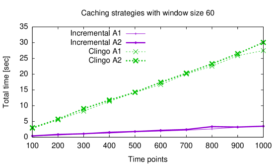
Figure 6: Runtime evaluation for increasing timepoints: Scenario A (Caching Strategy)

Figure 7: Runtime evaluation for increasing timepoints: Scenario B (Content Retrieval)

7 Related Work and Conclusion

In [Beck et al. (2015)], TMS techniques have been extended and applied for (plain) LARS, instead of reducing LARS to ASP. In contrast, the present approach does not primarily focus on model update, but incremental program update. Apart from work on Clingo mentioned earlier, alternatives to one-shot ASP were also considered by AlvianoDR14. The ASP approach of DoLL11 for stream reasoning calls the dlvhex solver; it has no incremental reasoning and cannot handle heavy data load. ETALIS [Anicic et al. (2012)] is a prominent rule formalism for complex event processing to reason about intervals for atomic events with a peculiar minimal model semantics. ETALIS is monotonic for a growing timeline (as such trivially incremental), and does not feature window mechanisms. StreamLog [Zaniolo (2012)] extends Datalog for single-model stream reasoning, where rules concluding about the past are excluded; neither windows nor incremental evaluation were considered. The DRed algorithm [Gupta et al. (1993)] for incremental Datalog update deletes all consequences of deleted facts and then adds all rederivable ones from the rest. It was adapted to RDF streams by Barbieri10, where tuples are tagged with an expiration time. RenP11 explored TMS techniques for ontology streams. However, windows and time reference were not considered in their monotonic setting. Towards incremental grounding, techniques as in [Lefèvre and Nicolas (2009), Palù et al. (2009), Dao-Tran et al. (2012)] might be considered.

Outlook. The algorithms we have presented center around the idea of incrementally adapting a model based on an incremental adjustment of a program. Our implementation indicates performance benefits arising from incremental evaluation. Developing techniques for full grounding on-the-fly in this context remains to be done. On the semantic side, notions of closeness between consecutive models and guarantees to obtain them are intriguing issues for future work.

Acknowledgements. We thank Roland Kaminski for providing guidance on the use of Clingo.

Appendix A Notes on the Use of Clingo

Reactive features. We established techniques that allow for incrementally updating a program $\hat{P}_{k}$ for time or count increment, where Alg. 3 identifies at each tick new rules $G^{+}$ that have to be added to the previous translation, and expired ones $G^{-}$ that must be deleted.

In search of existing systems that might allow such incremental program update, we considered the state-of-the-art ASP solver Clingo [Gebser et al. (2014)], which comes with an API for reactive/multi-shot solving. These functionalities are based on [Gebser et al. (2011)], have since evolved [Gebser et al. (2012), Gebser et al. (2014)] and successfully applied; e.g. viz. [Gebser et al. (2015)]. Unfortunately, for our purposes, control features in Clingo are not applicable.

First, the control features in Clingo allow addition of new rules, but not removal of existing ones. Technically, removing might be simulated by setting a designated switch atom to false. However, this approach would imply that the program grows over time. Second, we considered using reactive features as illustrated for Rule $r$ of Ex. 5, using a program part that is parameterized for stream variables, including that of tick $(t,c)$.

#program tick(t, c, v).
#external now(t).
#external cnt(c).
#external alpha_at(v,t).
high_at(t) :- w_time_2_alpha(v,t), t >= 18.
w_time_2_alpha(v,t) :- now(t), alpha_at(v,t).
w_time_2_alpha(v,t) :- now(t), alpha_at(v,t-1).
w_time_2_alpha(v,t) :- now(t), alpha_at(v,t-2).

However, this encoding is not applicable, since atoms in rule heads cannot be redefined, i.e., they cannot be grounded more than once.

Model update. For stratified programs (which have a unique model), repeatedly calling Clingo (by standard one-shot solving) on the encoded program $\hat{P}$ is a practical solution. However, when a program has multiple models, we then have no link between the output of successive ticks, i.e., the model may arbitrarily change. For instance, consider program

a :- not b, not c.  b :- not a, not c.  c :- not a, not b.

Using Clingo 5.1.0, the answer set of the program that is returned first is {a}, which remains an answer set if we add rule a :- not c. However, the first reported answer set now is {c}.

Appendix B Proofs

Proof for Lemma 1

Let $S=(T,\upsilon)$ be a stream that underlies tick stream $\dot{S}=(K,v)$, such that $K=\langle(t_{1},c_{1}),\dots,(t_{m},c_{m})\rangle$. By definition, $T=[t_{1},t_{m}]$ and $\upsilon(t)=\bigcup\{v(t,c)\mid(t,c)\in K\}$ for all $t\in T$. We recall that $\tau_{n}(S)$ (resp. $\tau_{n}(\dot{S})$) abbreviates $\tau_{n}(S,t_{m})$ (resp. $\tau_{n}(\dot{S},(t_{m},c_{m})$). Thus, by definition, $\tau_{n}(\dot{S})=(K^{\prime},v|_{K^{\prime}})$, where $K^{\prime}=\{(t^{\prime},c^{\prime})\in K\mid\max\{t_{1},t-n\}\leq t^{\prime}\leq t\}$, and $\tau_{n}(S)=(T^{\prime},\upsilon|_{T^{\prime}})$, where $T^{\prime}=[t^{\prime},t_{m}]$ and $t^{\prime}=\max\{t_{1},t-n\}$. We observe that $t^{\prime}$ is the minimal time point selected also in $K^{\prime}$, i.e., $K^{\prime}=\langle(t_{k},c_{k}),\dots,(t_{m},c_{m})\rangle$ implies $t_{k}=t^{\prime}$. It remains to show that $(\upsilon|_{T^{\prime}})(t)=\bigcup\{(v|_{K^{\prime}})(t,c)\mid(t,c)\in K^{\prime}\}$ for all $t\in T^{\prime}$. This is seen from the fact that neither $\tau_{n}(S)$ nor $\tau_{n}(\dot{S})$ drops any data within $T^{\prime}$. We conclude that $\tau_{n}(S)$ underlies $\tau_{n}(\dot{S})$.

Proof Sketch for Lemma 2

The argument is similar as for Lemma 1. The central observation is that a tick stream provides a more fine-grained control over the information available in streams by introducing an order on tuples in addition to the temporal order. Each time point in a stream is assigned a set of atoms, whereas each tick in a tick stream is assigned at most one atom. The tuple-based window function $\#_{n}$ always counts atoms backwards (from right end to left) and then selects the timeline $[t_{1},t]$ with the latest possible left time point $t_{1}$ required to capture $n$ atoms. While for tick streams, the order is unique, but multiple options exist for streams in general. If the tuple window $\#_{n}(S)$ is based on the order in which atoms appeared in $S$, then it selects the same atoms as $\#_{n}(\dot{S})$, and thus the same timeline. Consequently, $\#_{n}(S)$ underlies $\#_{n}(\dot{S})$.

Proof Sketch for Proposition 1

The desired correspondence is based on two translations: a LARS program $P$ (at a time $t$) into a logic program $\hat{P}=\mathit{LarsToAsp}(P,t)$ (due to Algorithm 1), and the encoding of a stream $S$ as set $\hat{S}$ of atoms. Given a fixed timeline $T$, we may view a stream $S=(T,\upsilon)$ as a set of pairs $\{(a({\mathbf{x}}),t)\mid a({\mathbf{x}})\in\upsilon(t),t\in T\}$. This is the essence of a stream encoding $\hat{S}$ for the tick stream $\dot{S}=(K,v)$; $\hat{S}$ includes the analogous time-pinned atoms: $\{a_{@}({\mathbf{x}},t)\mid a({\mathbf{x}})\in v(t,c),(t,c)\in K\}$. With respect to the correspondence, atoms of form $a_{\#}({\mathbf{x}},t,c)$, $\mathit{cnt}(c)$ and $\mathit{tick}(t,c)$ in $\hat{S}$ can be considered auxiliary, as well as the specific counts used in the tick pattern $K$ to obtain time-pinned atoms $a_{@}({\mathbf{x}},t)$. Counts play a role only for the specific selection of tuple-based windows, which are assumed to reflect the order of the tick stream. Thus, we may view a stream encoding $\hat{S}$ essentially as a different representation of stream $S$; additional atoms can be abstracted away as they have no correspondence in the original LARS stream or program. We thus consider only the time-pinned atoms in an encoded stream to read off a LARS stream.

Thus, it remains to argue the soundness of the transformation $\mathit{LarsToAsp}$, which returns a program of form $Q\cup R\cup\{\mathit{now}(t)\}$, where $\mathit{now}(t)$ is auxiliary. The set $Q$ simply identifies time-pinned atoms $a_{@}({\mathbf{X}},\dot{N})$ with $a({\mathbf{X}})$ in case $\dot{N}$ is the current time point. This is the information provided by predicate $\mathit{now}$ for which a unique atom exists. Thus, $Q$ ensures that a time-pinned atom $a_{@}({\mathbf{x}},t)$ is available if $a({\mathbf{x}},t)$ is derived, and vice versa; $Q$ thereby only accounts for redundant representations of atoms that currently hold.

Towards $R$, we get the translation by the function $\mathit{larsToAspRules}$ which returns a set of encoded rules for every LARS rule $r$. First, the $\mathit{baseRule}$ is the corresponding ASP rule, which introduces a new symbol $\mathit{atm}(e)$ for every extended atom in the rule that is not an ordinary atom. In order to ensure that the base rule $\hat{r}$ fires in an interpretation just if the original rule $r$ fires in the corresponding interpretation of program $P$, for each body element $\mathit{atm}(e)$ in $\hat{r}$ the set of rules to derive $\mathit{atm}(e)$ in lines (14)-(21) is provided; the correspondence between $@_{T}a({\mathbf{X}})$ and $a_{@}({\mathbf{X}},T)$ is already given by construction. Thus, each interpretation stream $I\supseteq D$ for $P$ has a corresponding interpretation $\hat{I}$ for $\mathit{LarsToAsp}(P)$ in which besides the time-pinned atoms the atoms $\mathit{atm}(e)$ and $\mathit{spoil}_{e}({\mathbf{X}})$ occur depending on support from (i.e., firing) of the rules in (14)-(21), such that they correctly reflect the value of the window atoms $e$ in $I$.

As each atom in an answer of an ordinary ASP program must derived by a rule, it is not hard to see that every answer set of $\hat{P}=\mathit{LarsToAsp}(P,t)\cup\hat{D}$ is of the form $\hat{I}$, where $I\supseteq D$ is an interpretation stream for $D$. We thus need to show the following: $I\in AS(P,D,t)$ holds iff $\hat{I}$ is an answer set of $\hat{P}$. We do this for ground $P$ (the extension to non-ground $P$ is straightforward).

($\Rightarrow$) For the only-if direction, we show that if $I\in AS(P,D,t)$, that is, $I$ is a minimal model for the reduct $P^{M,t}$ where $M=\langle I,W,B\rangle$, then (i) $\hat{I}$ is a model of the reduct $\hat{P}^{\hat{I}}$, and (ii) no interpretation $J^{\prime}\subset\hat{I}$ is a model of $\hat{P}^{\hat{I}}$. As for (i), we can concentrate by construction of $\hat{I}$ on the base rules $\hat{r}=\mathit{baseRule}(r)$ in $\hat{P}^{\hat{I}}$ (all other rules will be satisfied). If $\hat{I}$ satisfies $\mathit{B}(\hat{r})$, then by construction $I$ satisfies $\mathit{B}(r)$; as $I$ is a model of $P^{M,t}$, it follows that $I$ satisfies $\mathit{H}(r)$; but then, by construction, $\hat{I}$ satisfies $\mathit{H}(\hat{r})$. As for (ii), we assume towards a contradiction that some $J^{\prime}\subset\hat{I}$ satisfies $\hat{P}^{\hat{I}}$. We then consider the stream $J\supseteq D$ that is induced by $J^{\prime}$, and any rule $r$ in the reduct $P^{M,t}$. If $J$ does not satisfy $\mathit{B}(r)$, then $J$ satisfies $r$; otherwise, if $J$ satisfies $\mathit{B}(r)$, then as $\hat{r}$ is in the reduct $\hat{P}^{\hat{I}}$, we have that $\hat{I}$ falsifies each atom $\mathit{atm}(e)$ in $\mathit{B}^{-}(\hat{r})$, and as $J^{\prime}\subset\hat{I}$, also $J^{\prime}$ falsifies each such $\mathit{atm}(e)$. Furthermore, as $J$ satisfies each atom $e\in\mathit{B}^{+}(r)$, from the rules for $\mathit{atm}(e)$ among (14)-(21) in the reduct $\hat{P}^{\hat{I}}$ we obtain that $J^{\prime}$ satisfies each atom $\mathit{atm}(e)$ in $\mathit{B}^{+}(\hat{r})$. That is, $J^{\prime}$ satisfies $\mathit{B}(\hat{r})$. As $J^{\prime}$ satisfies $\hat{r}$, we then obtain that $J^{\prime}$ satisfies $\mathit{H}(\hat{r})$. The latter means that $J$ satisfies $\mathit{H}(r)$, and thus $J$ satisfies $r$. As $r$ was arbitrary from the reduct $P^{M,t}$, we obtain that $J\subset I$ is a model of $P^{M,t}$; this however contradicts that $I$ is a minimal model of $P^{M,t}$, and thus (ii) holds.

($\Leftarrow$) For the if direction, we argue similarly. Consider an answer set $\hat{I}$ of $\hat{P}$. To show that $I\in AS(P,D,t)$, we establish that (i) $I$ is a model of $P^{M,t}$ and (ii) no model $J\subset I$ of $P^{M,t}$ exists. As for (i), since in $\hat{I}$ the atoms $\mathit{atm}(e)$ correctly reflect the value of the window atoms $e$ in $I$, for each $r$ in $P^{M,t}$ the rule $\hat{r}=\mathit{baseRule}(r)$ is in $\hat{P}^{\hat{I}}$; as $\hat{I}$ satisfies $\hat{r}$, we conclude that $I$ satisfies $r$. As for (ii), we show that every model $J$ of $P^{M,t}$ must contain $I$, which then proves the result.

To establish this, we use the fact that $\hat{I}$ can be generated by a sequence $\rho=r_{1},r_{2},r_{3}\ldots,r_{k}$ of rules from $\hat{P}^{\hat{I}}$ with distinct heads such that (a) $\hat{I}=\{\mathit{H}(r_{1}),\ldots\mathit{H}(r_{k})\}=:\hat{I}_{k}$ and (b) $\hat{I}_{i-1}=\{\mathit{H}(r_{1}),\ldots,\mathit{H}(r_{i-1})\}$ satisfies $\mathit{B}^{+}(r_{i})$, for every $i=1,\ldots,k$.

In that, we use the assertion that no cyclic positive dependencies through time-based window atoms $\boxplus^{n}\Box a$ occur. Formally, positive dependency is defined as follows: an atom $@_{t_{1}}b$ positively depends on an atom $@_{t_{2}}a$ in a ground program $P$ at $t$, if some rule $r\in P$ exists with $\mathit{H}(r)=@_{t_{1}}b$ and such that either (a) $@_{t_{2}}a\in\mathit{B}^{+}(r)$, or (b) $\boxplus^{n}@_{t_{2}}a\in\mathit{B}^{+}(r)$ or (c) $\boxplus^{n}\star a\in\mathit{B}^{+}(r)$, $\star\in\{\Box,\Diamond\}$, where in (b) and (c) $t_{2}\in[t-n,t]$ holds. As in $\mathit{LarsToAsp}(P,t)$, all ordinary atoms $a$ are here viewed as $@_{t}a$. A cyclic positive dependency through $\boxplus^{n}\Box a$ is then a sequence $@_{t_{0}}a_{0}$, $@_{t_{1}}a_{1}$, …, $@_{t_{k}}a_{k}$, $k\geq 1$, such that $@_{t_{i}}a_{i}$ positively depends on ${@_{t_{(i+1)\mod k}}\,a_{(i+1)\mod k}}$, for all $i=0,\ldots,k$ and $a_{0}=b$ and $a_{1}=a$ for case (c) with $\star=\Box$.

Given that no positive cyclic dependencies through atoms $\boxplus^{n}\Box a$ occur in $P$ at $t$, and thus in $P^{M,t}$, we can w.l.o.g. assume that whenever $r_{i}$ in $\rho$ has a head $\omega_{e}$ for a window atom $e=\boxplus^{n}\Box a$, each rule $r_{j}$ in $\rho$ with a head $a_{@}(t^{\prime})$, where $t^{\prime}\in[t-n,t]$, precedes $r_{i}$, i.e., $j<i$ holds.

By induction on $i\geq 1$, we can now show that if $\mathit{H}(r_{i})=\mathit{atm}(e)$, then every model $J$ of $P^{M,t}$ must satisfy $e$; consequently, at $i=k$, $J$ must contain $I$. From the form of the rules $\mathit{baseRule}(r)$ and $\mathit{windowRules}(e)$, the correspondence between $\hat{P}^{\hat{I}}$ and $P^{M,t}$, and the fact that the external data are facts, only the case $e=\boxplus^{n}\Box a({\mathbf{X}})$ needs a further argument. Now if $r_{i}$ is the rule $\omega_{e}\leftarrow a({\mathbf{X}}),\operatorname{not}\,\mathit{spoil}_{e}({\mathbf{X}})$ on line (16), then $\hat{I}$ must satisfy $a$ and falsify $\mathit{spoil}_{e}({\mathbf{X}})$; in turn, every $a_{@}(t^{\prime},{\mathbf{X}})$ must be true in $\hat{I}$, for $t^{\prime}\in[t-n,t]$. From the induction hypothesis, we obtain that $@_{t^{\prime}}a({\mathbf{X}})$ is true in every model $J$ of $P^{M,t}$, $t^{\prime}\in[t-n,t]$, and thus $e=\boxplus^{n}\Box a({\mathbf{X}})$ is true as well. This proves the claim and concludes the proof of the if-case, which in turn establishes the claimed correspondence between $AS(P,D,t)$ and the answer sets of $\hat{P}=\mathit{LarsToAsp}(P,t)\cup\hat{D}$.

Remark. The condition on cyclic positive dependencies excludes that rules $b\leftarrow\boxplus^{n}\Box a$ and $a\leftarrow b$ occur jointly in a program. A stricter notion of dependency that allows for co-occurrence is to request in (c) for $\star=\Box$ in addition $t_{2}<t$; then e.g. any LARS program where the rule heads are ordinary atoms is allowed, and Proposition 1 remains valid.

Proof Sketch for Proposition 2

Assume a LARS program $P$ and two tick data streams $D=(K,v)$ and $D^{\prime}=(K^{\prime},v^{\prime})$ at tick $(t_{m},c_{m})$ such that $D^{\prime}\subseteq D$ and $K^{\prime}=\langle(t_{k},c_{k}),\dots,(t_{m},c_{m})\rangle$. Furthermore, assume that (*) all atoms/time points accessible from any window in $P$ are included in $D^{\prime}$. We want to show $AS^{I}(\hat{P}_{D,m})=AS^{I}(\hat{P}_{D^{\prime},m})$. The central observation is that rules need to fire in order for intensional atoms to be included in the answer set, and that no rules can fire based on outdated ticks. Thus, these ticks can also be dropped.

In more detail, we assume $AS^{I}(\hat{P}_{D,m})\neq AS^{I}(\hat{P}_{D^{\prime},m})$ towards a contradiction. That is to say, a difference in evaluation arises based on data in $D\setminus D^{\prime}$, i.e., atoms appearing before tick $(t_{k},c_{k})$. Consider any extended atom $e$ of a (LARS) rule $r\in P$, where the body holds only for one of the two encodings (in the same partial interpretation). Due to the assumption (*), we can exclude a difference arising from a window atom of form $\boxplus^{w}\star a$, $\star\in\{\Diamond,\Box,@_{T}\}$.

If $e$ is an atom $a$, it holds in $\hat{P}_{D,m}$ iff it holds in $\hat{P}_{D^{\prime},m}$ since an ordinary atom in the answer set of the encoding corresponds to an atom holding at the current time point, and both $D$ and $D^{\prime}$ include the current time point.

The last option is $e=@_{T}a$, which may reach back beyond $(t_{k},c_{k})$ but is viewed in the incremental encoding as syntactic shortcut for $\boxplus^{\infty}@_{T}a$. That is, in this case we have $D^{\prime}=D$ and thus the encodings coincide.

We conclude that assuming $AS^{I}(\hat{P}_{D,m})\neq AS^{I}(\hat{P}_{D^{\prime},m})$ is contradictory due to these observations. Spelling out the details fully involves essentially a case distinction on the incremental window encodings and arguing about the relationship between $(t_{k},c_{k})$, the respective expiration annotations, and the fact that rules accessing atoms at ticks before $(t_{k},c_{k})$ are have already expired.

Proof Sketch for Proposition 3

We argue based on the commonalities and differences of the static encoding $\hat{P}\cup\hat{D}$ and the incremental encoding $\hat{P}_{D,m}$. Instead of body predicates $\mathit{now}(\dot{N})$ and $\mathit{cnt}(\dot{C})$, that are instantiated in $\hat{P}\cup\hat{D}$ due to the predicates $\mathit{now}(t)$ and $\mathit{cnt}(c)$, $\hat{P}_{D,m}$ directly uses the instantiations of tick variables. In both encodings, the window atom is associated with a set of rules that needs to model the temporal quantifier ($\Diamond$,$\Box$,$@_{t}$) in the correct range of ticks as expressed by the LARS window atom. This window always includes the last tick. While $\hat{P}\cup\hat{D}$ is based on a complete definition how far the window extends, $\hat{P}_{D,m}$ updates this definition tick by tick. In particular, the oldest tick that is not covered by the window anymore corresponds to the expiration annotation in $\hat{P}_{D,m}$.

The case $\boxplus^{n}\Diamond a({\mathbf{X}})$ is as follows: in the static rule encoding,

$$\omega_{e}({\mathbf{X}})\leftarrow\mathit{now}(\dot{N}),a_{@}({\mathbf{X}},T)\,,$$

given $\mathit{now}(t)$, time variable $T$ will be grounded with $t-n,\dots,t-0$. That is, we get a set of rules

$$\begin{array}[]{lrcl}(r_{0})&\omega_{e}({\mathbf{X}})&\leftarrow&\mathit{now}(t),a_{@}({\mathbf{X}},t)\\ &&\vdots\\ (r_{n})&\omega_{e}({\mathbf{X}})&\leftarrow&\mathit{now}(t),a_{@}({\mathbf{X}},t-n)\,,\end{array}$$

where arguments ${\mathbf{X}}$ will be grounded due to data and inferences. We observe that $(r_{0})$ is the rule that is inserted to the incremental program $\hat{P}_{D,m}$ at time $t$ (minus predicate $\mathit{now}(t)$, since in $\hat{P}_{D,m}$ variable $T$ is instantiated directly with $t$ to obtain $a_{@}({\mathbf{X}},t)$), and all rules up to $r_{n}$ remain from previous calls to $\mathit{IncrementalRules}$. Rule $r_{n}$ will expire at $t+1$, i.e., the exact time when it will not be included in $\hat{P}\cup\hat{D}$ anymore. The cases for $\boxplus^{n}@_{T}a({\mathbf{X}}),\boxplus^{n}\Box a({\mathbf{X}}),\boxplus^{\#n}\Diamond a({\mathbf{X}})$ and $\boxplus^{\#n}@_{T}a({\mathbf{X}})$ are analogous; the remaining case $\boxplus^{\#n}\Box a({\mathbf{X}})$ has been argued earlier.

Finally, $\hat{P}_{D,m}$ includes a stream encoding, which is also incrementally maintained: at each tick $(t,c)$ the tick atom $\mathit{tick}(t,c)$ is added, and in case of a count increment, the time-pinned atom $a_{@}({\mathbf{X}},t)$ and the tick-pinned atoms $a_{\#}({\mathbf{X}},t,c)$ are added to $\hat{P}_{D,m}$ as in $\hat{D}$. This way, we have a full correspondence with the static stream encoding $\hat{D}$.

Thus, at every tick $(t,c)$, $\hat{P}\cup\hat{D}$ and $\hat{P}_{D,m}$ have the same data and express the same evaluations. Disregarding auxiliary atoms, we conclude that their answer sets coincide.

Proof Sketch for Theorem 1

Given a LARS program $P$, a tick data stream $D=(K,v)$ at tick $(t,c)$ by Prop. 1 $S$ is an answer stream of $P$ for $D$ at $t$ iff $\hat{S}$ is an answer set of $\hat{P}\cup\hat{D}$, where $\hat{P}=\mathit{LarsToAsp(P,t)}$. By Prop. 3, for any set $X$ we have that $X\cup\{\mathit{now}(t),\mathit{cnt}(c)\}$ is an answer set of $\hat{P}\cup\hat{D}$ iff $X$ is an answer set of $\hat{P}_{D,m}$ (modulo auxiliary atoms). In particular this holds for $X=\hat{S}$. As $\{\mathit{now}(t),\mathit{cnt}(c)\}\subseteq\hat{S}$, we obtain that $S$ is an answer stream of $P$ for $D$ at $t$ iff $\hat{S}$ is an answer set of $\hat{P}_{D,m}$, which is the result.

Appendix C Details of Evaluation Results

(See pages 1–8.)

Table 1: Results for A1. Variable window size $n$. Results for 1000 timepoints in seconds.

	Clingo			Incremental
$n$	$t_{\mathit{total}}$	$t_{\mathit{init}}$	$t_{\mathit{tick}}$	$t_{\mathit{total}}$	$t_{\mathit{init}}$	$t_{\mathit{tick}}$
20	14.296	0.017	0.014	2.638	0.016	0.002
40	20.526	0.018	0.02	3.006	0.018	0.002
80	34.491	0.025	0.034	2.938	0.018	0.002
120	49.249	0.027	0.049	3.439	0.019	0.003
160	64.661	0.028	0.064	3.554	0.017	0.003
200	79.105	0.036	0.079	3.674	0.018	0.003

Table 2: Results for A2. Variable window size $n$. Runtime for 1000 timepoints in seconds.

	Clingo			Incremental
$n$	$t_{\mathit{total}}$	$t_{\mathit{init}}$	$t_{\mathit{tick}}$	$t_{\mathit{total}}$	$t_{\mathit{init}}$	$t_{\mathit{tick}}$
20	15.259	0.02	0.015	2.869	0.016	0.002
40	23.123	0.02	0.023	3.201	0.018	0.003
80	35.962	0.022	0.035	3.365	0.019	0.003
120	49.068	0.026	0.049	3.547	0.02	0.003
160	61.983	0.03	0.061	3.842	0.018	0.003
200	80.899	0.036	0.08	3.7	0.019	0.003

Table 3: Results for A1. Variable timepoints $\mathit{tp}$. Runtime for window size $n=60$ in seconds.

	Clingo			Incremental
$\mathit{tp}$	$t_{\mathit{total}}$	$t_{\mathit{init}}$	$t_{\mathit{tick}}$	$t_{\mathit{total}}$	$t_{\mathit{init}}$	$t_{\mathit{tick}}$
100	2.78	0.026	0.027	0.368	0.023	0.003
200	5.49	0.022	0.027	0.674	0.02	0.003
300	8.269	0.022	0.027	1.072	0.026	0.003
400	11.379	0.026	0.028	1.307	0.02	0.003
500	14.192	0.024	0.028	1.695	0.017	0.003
600	16.709	0.023	0.027	1.945	0.02	0.003
700	20.049	0.021	0.028	2.217	0.017	0.003
800	22.534	0.021	0.028	2.627	0.018	0.003
900	25.892	0.024	0.028	3.183	0.022	0.003
1000	27.501	0.021	0.027	3.42	0.021	0.003

Table 4: Results for A2. Variable timepoints $\mathit{tp}$. Runtime for window size $n=60$ in seconds.

	Clingo			Incremental
$\mathit{tp}$	$t_{\mathit{total}}$	$t_{\mathit{init}}$	$t_{\mathit{tick}}$	$t_{\mathit{total}}$	$t_{\mathit{init}}$	$t_{\mathit{tick}}$
100	2.998	0.026	0.029	0.418	0.019	0.003
200	5.727	0.023	0.028	0.89	0.017	0.004
300	9.06	0.026	0.03	1.097	0.021	0.003
400	11.783	0.021	0.029	1.563	0.02	0.003
500	14.26	0.021	0.028	1.81	0.017	0.003
600	17.439	0.02	0.029	2.181	0.021	0.003
700	20.321	0.021	0.028	2.438	0.018	0.003
800	23.3	0.02	0.029	3.371	0.02	0.004
900	26.51	0.021	0.029	3.22	0.018	0.003
1000	30.077	0.024	0.03	3.5	0.019	0.003

Table 5: Results for B1. Variable window size $n$. Runtime in seconds for 1000 timepoints.

	Clingo			Incremental
$n$	$t_{\mathit{total}}$	$t_{\mathit{init}}$	$t_{\mathit{tick}}$	$t_{\mathit{total}}$	$t_{\mathit{init}}$	$t_{\mathit{tick}}$
20	26.158	0.018	0.026	15.641	0.292	0.015
40	55.898	0.021	0.055	16.726	0.315	0.016
80	425.853	0.019	0.425	21.135	0.299	0.02
120	-	-	-	25.909	0.304	0.025
160	-	-	-	30.659	0.363	0.03
200	-	-	-	33.541	0.306	0.033

Table 6: Results for B2. Variable window size $n$. Runtime for 1000 timepoints in seconds.

	Clingo			Incremental
$n$	$t_{\mathit{total}}$	$t_{\mathit{init}}$	$t_{\mathit{tick}}$	$t_{\mathit{total}}$	$t_{\mathit{init}}$	$t_{\mathit{tick}}$
20	24.138	0.018	0.024	34.717	0.292	0.033
40	38.478	0.019	0.038	35.744	0.333	0.034
80	71.827	0.024	0.071	25.767	0.298	0.025
120	104.723	0.023	0.104	33.788	0.29	0.033
160	148.257	0.031	0.148	31.1	0.303	0.03
200	181.991	0.028	0.181	37.612	0.33	0.036

Table 7: Results for B1. Variable timepoints $\mathit{tp}$. Window size $n=60$ in seconds.

	Clingo			Incremental
$\mathit{tp}$	$t_{\mathit{total}}$	$t_{\mathit{init}}$	$t_{\mathit{tick}}$	$t_{\mathit{total}}$	$t_{\mathit{init}}$	$t_{\mathit{tick}}$
100	8.57	0.026	0.085	1.895	0.32	0.015
200	16.392	0.022	0.081	3.971	0.293	0.018
300	31.568	0.022	0.105	6.82	0.475	0.021
400	40.927	0.025	0.102	8.518	0.332	0.02
500	55.313	0.021	0.11	10.64	0.351	0.02
600	69.548	0.021	0.115	12.816	0.353	0.02
700	-	-	-	15.773	0.333	0.021
800	-	-	-	16.756	0.318	0.02
900	-	-	-	16.96	0.298	0.018
1000	-	-	-	18.602	0.298	0.018

Table 8: Results for B2. Variable timepoints $\mathit{tp}$. Window size $n=60$ in seconds.

	Clingo			Incremental
$\mathit{tp}$	$t_{\mathit{total}}$	$t_{\mathit{init}}$	$t_{\mathit{tick}}$	$t_{\mathit{total}}$	$t_{\mathit{init}}$	$t_{\mathit{tick}}$
100	4.974	0.029	0.049	1.838	0.299	0.015
200	10.06	0.021	0.05	3.982	0.304	0.018
300	15.023	0.02	0.049	6.126	0.359	0.019
400	20.574	0.019	0.051	9.062	0.29	0.021
500	26.075	0.02	0.052	11.625	0.289	0.022
600	31.68	0.02	0.052	14.974	0.297	0.024
700	36.35	0.02	0.051	18.301	0.29	0.025
800	42.391	0.021	0.052	22.947	0.286	0.028
900	48.254	0.021	0.053	28.979	0.366	0.031
1000	54.35	0.02	0.054	28.993	0.334	0.028

References

- Alviano et al. (2014) Alviano, M., Dodaro, C., and Ricca, F. 2014. Anytime computation of cautious consequences in answer set programming. TPLP 14, 4-5, 755–770.
- Anicic et al. (2012) Anicic, D., Rudolph, S., Fodor, P., and Stojanovic., N. 2012. Stream reasoning and complex event processing in ETALIS. Semantic Web Journal.
- Babu and Widom (2001) Babu, S. and Widom, J. 2001. Continuous queries over data streams. SIGMOD Record 3, 30, 109–120.
- Barbieri et al. (2010) Barbieri, D. F., Braga, D., Ceri, S., Valle, E. D., and Grossniklaus, M. 2010. Incremental reasoning on streams and rich background knowledge. In The Semantic Web: Research and Applications, 7th Extended Semantic Web Conference, ESWC 2010, Heraklion, Crete, Greece, May 30 - June 3, 2010, Proceedings, Part I, L. Aroyo, G. Antoniou, E. Hyvönen, A. ten Teije, H. Stuckenschmidt, L. Cabral, and T. Tudorache, Eds. Lecture Notes in Computer Science, vol. 6088. Springer, 1–15.
- Beck (2017) Beck, H. 2017. Reviewing Justification-based Truth Maintenance Systems from a Logic Programming Perspective. Tech. Rep. INFSYS RR-1843-17-02, Institute of Information Systems, TU Vienna. July.
- Beck et al. (2017) Beck, H., Bierbaumer, B., Dao-Tran, M., Eiter, T., Hellwagner, H., and Schekotihin, K. 2017. Stream Reasoning-Based Control of Caching Strategies in CCN Routers. In Proceedings of the IEEE International Conference on Communications, May 21-25, 2017, Paris, France.
- Beck et al. (2015) Beck, H., Dao-Tran, M., and Eiter, T. 2015. Answer update for rule-based stream reasoning. In Proceedings of the 24th International Joint Conference on Artificial Intelligence (IJCAI-15), July 25-31, 2015, Buenos Aires, Argentina, Q. Yang and M. Wooldridge, Eds. AAAI Press/IJCAI, 2741–2747.
- Beck et al. (2015) Beck, H., Dao-Tran, M., Eiter, T., and Fink, M. 2015. LARS: A logic-based framework for analyzing reasoning over streams. In Proceedings 29th Conference on Artificial Intelligence (AAAI ’15), January 25-30, 2015, Austin, Texas, USA, B. Bonet and S. Koenig, Eds. AAAI Press, 1431–1438.
- Dao-Tran et al. (2012) Dao-Tran, M., Eiter, T., Fink, M., Weidinger, G., and Weinzierl, A. 2012. Omiga : An open minded grounding on-the-fly answer set solver. In Logics in Artificial Intelligence - 13th European Conference, JELIA 2012, Toulouse, France, September 26-28, 2012. Proceedings, L. F. del Cerro, A. Herzig, and J. Mengin, Eds. Lecture Notes in Computer Science, vol. 7519. Springer, 480–483.
- Della Valle et al. (2009) Della Valle, E., Ceri, S., van Harmelen, F., and Fensel, D. 2009. It’s a streaming world! reasoning upon rapidly changing information. IEEE Intelligent Systems 24, 83–89.
- Do et al. (2011) Do, T. M., Loke, S. W., and Liu, F. 2011. Answer set programming for stream reasoning. In Advances in Artificial Intelligence - 24th Canadian Conference on Artificial Intelligence, Canadian AI 2011, St. John’s, Canada, May 25-27, 2011. Proceedings, C. J. Butz and P. Lingras, Eds. Lecture Notes in Computer Science, vol. 6657. Springer, 104–109.
- Doyle (1979) Doyle, J. 1979. A Truth Maintenance System. Artif. Intell. 12, 3, 231–272.
- Elkan (1990) Elkan, C. 1990. A rational reconstruction of nonmonotonic truth maintenance systems. Artif. Intell. 43, 2, 219–234.
- Gebser et al. (2012) Gebser, M., Grote, T., Kaminski, R., Obermeier, P., Sabuncu, O., and Schaub, T. 2012. Stream reasoning with answer set programming: Preliminary report. In Principles of Knowledge Representation and Reasoning: Proceedings of the Thirteenth International Conference, KR 2012, Rome, Italy, June 10-14, 2012, G. Brewka, T. Eiter, and S. A. McIlraith, Eds. AAAI Press.
- Gebser et al. (2011) Gebser, M., Grote, T., Kaminski, R., and Schaub, T. 2011. Reactive answer set programming. In Logic Programming and Nonmonotonic Reasoning - 11th International Conference, LPNMR 2011, Vancouver, Canada, May 16-19, 2011. Proceedings, J. P. Delgrande and W. Faber, Eds. Lecture Notes in Computer Science, vol. 6645. Springer, 54–66.
- Gebser et al. (2014) Gebser, M., Kaminski, R., Kaufmann, B., and Schaub, T. 2014. Clingo = ASP + control: Preliminary report. In Technical Communications of the Thirtieth International Conference on Logic Programming (ICLP’14), M. Leuschel and T. Schrijvers, Eds. Vol. arXiv:1405.3694v1. Theory and Practice of Logic Programming, Online Supplement.
- Gebser et al. (2015) Gebser, M., Kaminski, R., Obermeier, P., and Schaub, T. 2015. Ricochet robots reloaded: A case-study in multi-shot ASP solving. In Advances in Knowledge Representation, Logic Programming, and Abstract Argumentation - Essays Dedicated to Gerhard Brewka on the Occasion of His 60th Birthday, T. Eiter, H. Strass, M. Truszczynski, and S. Woltran, Eds. Lecture Notes in Computer Science, vol. 9060. Springer, 17–32.
- Gupta et al. (1993) Gupta, A., Mumick, I. S., and Subrahmanian, V. S. 1993. Maintaining views incrementally. ACM SIGMOD International Conference on Management of Data, 157–166.
- Lefèvre and Nicolas (2009) Lefèvre, C. and Nicolas, P. 2009. The first version of a new ASP solver : Asperix. In Logic Programming and Nonmonotonic Reasoning, 10th International Conference, LPNMR 2009, Potsdam, Germany, September 14-18, 2009. Proceedings, E. Erdem, F. Lin, and T. Schaub, Eds. Lecture Notes in Computer Science, vol. 5753. Springer, 522–527.
- Palù et al. (2009) Palù, A. D., Dovier, A., Pontelli, E., and Rossi, G. 2009. Answer set programming with constraints using lazy grounding. In Logic Programming, 25th International Conference, ICLP 2009, Pasadena, CA, USA, July 14-17, 2009. Proceedings, P. M. Hill and D. S. Warren, Eds. Lecture Notes in Computer Science, vol. 5649. Springer, 115–129.
- Phuoc et al. (2011) Phuoc, D. L., Dao-Tran, M., Parreira, J. X., and Hauswirth, M. 2011. A native and adaptive approach for unified processing of linked streams and linked data. In ISWC (1). 370–388.
- Ren and Pan (2011) Ren, Y. and Pan, J. Z. 2011. Optimising ontology stream reasoning with truth maintenance system. In Proceedings of the 20th ACM Conference on Information and Knowledge Management, CIKM 2011, Glasgow, United Kingdom, October 24-28, 2011, C. Macdonald, I. Ounis, and I. Ruthven, Eds. ACM, 831–836.
- Spring et al. (2004) Spring, N. T., Mahajan, R., Wetherall, D., and Anderson, T. E. 2004. Measuring ISP topologies with rocketfuel. IEEE/ACM Trans. Netw. 12, 1, 2–16.
- Zaniolo (2012) Zaniolo, C. 2012. Logical foundations of continuous query languages for data streams. In Datalog. 177–189.