Certification and Quantification of Multilevel Quantum Coherence
Abstract
Quantum coherence, present whenever a quantum system exists in a superposition of multiple classically distinct states, marks one of the fundamental departures from classical physics. Quantum coherence has recently been investigated rigorously within a resource-theoretic formalism. However, the finer-grained notion of multilevel coherence, which explicitly takes into account the number of superposed classical states, has remained relatively unexplored. A comprehensive analysis of multi-level coherence, which acts as the single-party analogue to multi-partite entanglement, is essential for understanding natural quantum processes as well as for gauging the performance of quantum technologies. Here we develop the theoretical and experimental groundwork for characterizing and quantifying multilevel coherence. We prove that non-trivial levels of purity are required for multilevel coherence, as there is a ball of states around the maximally mixed state that do not exhibit multilevel coherence in any basis. We provide a simple necessary and sufficient analytical criterion to verify the presence of multilevel coherence, which leads to a complete classification of multilevel coherence for three-level systems. We present the robustness of multilevel coherence, a bona fide quantifier which we show to be numerically computable via semidefinite programming and experimentally accessible via multilevel coherence witnesses, which we introduce and characterize. We further verify and lower-bound the robustness of multilevel coherence by performing a semi-device-independent phase discrimination task, which is implemented experimentally with four-level quantum probes in a photonic setup. Our results contribute to understanding the operational relevance of genuine multilevel coherence, also by demonstrating the key role it plays in enhanced phase discrimination—a primitive for quantum communication and metrology—and suggest new ways to reliably and effectively test the quantum behaviour of physical systems.
Quantum coherence manifests whenever a quantum system is in a superposition of classically distinct states, such as different energy levels or spin directions. Formally, a quantum state displays coherence111For brevity, we will omit the qualifier “quantum” in the following., whenever it is described by a density matrix that is not diagonal with respect to the relevant orthogonal basis of classical states Streltsov et al. (2017). In this sense, coherence underpins virtually all quantum phenomena, yet has only recently been characterised formally Aberg (2006); Baumgratz et al. (2014); Marvian and Spekkens (2016). Coherence is now recognised as a fully-fledged resource and studied in the general framework of quantum resource theories Coecke et al. (2016); Horodecki and Oppenheim (2013); Brandão and Gour (2015); Streltsov et al. (2017). This has led to a menagerie of possible ways to quantify coherence in a quantum system Baumgratz et al. (2014); Napoli et al. (2016); Piani et al. (2016); Yuan et al. (2015); Winter and Yang (2016); Biswas et al. (2017); Streltsov et al. (2015); Chitambar et al. (2016); Adesso et al. (2016); Marvian et al. (2016); Girolami (2014); Streltsov et al. (2017); Ren et al. (2017), along with an intense analysis of how coherence plays a role in fundamental physics, e.g., in quantum thermodynamics Kammerlander and Anders (2016); Uzdin et al. (2015), and in operational tasks relevant to quantum technologies, including quantum algorithms and quantum metrology Hillery (2016); Napoli et al. (2016); Piani et al. (2016); Marvian et al. (2016); Giorda and Allegra (2018); Zhang et al. (2017); Ren et al. (2017); Braun et al. (2017).
Despite a great deal of recent progress, however, the majority of current literature focuses on a rather coarse-grained description of coherence, which is ultimately insufficient to reach a complete understanding of the fundamental role of quantum superposition in the aforementioned tasks. To overcome such limitations, one needs to take into consideration the number of classical states in coherent superposition—contrasted to the simpler question of whether any non-trivial superposition exists—which gives rise to the concept of multilevel quantum coherence Levi and Mintert (2014); Sperling and Vogel (2015); Killoran et al. (2016). Similarly to the existence of different degrees of entanglement in multi-partite systems, going well beyond the mere presence or absence of entanglement and corresponding to different capabilities in quantum technologies Horodecki et al. (2009); Gühne and Tóth (2009), one can then identify and study a rich structure for multilevel coherence. Deciphering this structure can yield a tangible impact on many areas of physics, such as condensed matter, statistical mechanics and transfer phenomena in many-body systems Levi and Mintert (2014); Li et al. (2012); Lostaglio et al. (2015); Scholes et al. (2017). For example, for understanding the role of coherence in the function of complex biological molecules, such as those found in light harvesting, it will be crucial to differentiate between pairwise coherence among the various sites in the molecule, and genuine multilevel coherence across many sites Scholes et al. (2017); Witt and Mintert (2013); Scholak et al. (2011); Tiersch et al. (2012). In quantum computation, large superpositions of computational basis states need to be generated and effective benchmarking of such devices require proper tools to certify and quantify multilevel coherence.
Recent works have presented initial approaches to measuring the amount of multilevel coherence Chin (2017a), as well as schemes to convert it into bipartite and genuine multi-partite entanglement, enabling the fruitful use of entanglement theory tools to study coherence itself Regula et al. (2017); Killoran et al. (2016); Chin (2017b). Nonetheless, an all-inclusive systematic framework for the characterization, certification, and quantification of multilevel coherence is still lacking.
Here we construct and present such a theoretical framework for multilevel coherence and apply it to the experimental verification and quantification of multilevel coherence in a quantum optical setting. We begin by developing a resource theory of multilevel coherence, in particular providing a new characterisation of the sets of multilevel coherence-free states (see Fig. 1a) and free operations, rigorously unfolding the hierarchy of multilevel coherence. We present analytical criteria for multilevel coherence, which lead to a complete classification of multilevel coherence for three-level systems, and which establish lower bounds on the purity required to exhibit multilevel coherence. We then formalise the robustness of multilevel coherence and show that it is an efficiently computable measure, which is experimentally accessible through multilevel coherence witnesses. Using photonic four-dimensional systems we demonstrate how to quantify, witness, and bound multilevel coherence experimentally. We prove that multilevel coherence, quantified by our robustness measure, has a natural operational interpretation as a fundamental resource for quantum phase discrimination Napoli et al. (2016); Piani et al. (2016), a cornerstone task for quantum metrology and communication technologies Gottesman (1999); Barnett and Croke (2009). In turn, we show how to exploit this task to experimentally lower-bound the robustness of multilevel coherence of an unknown quantum state in a semi-device-independent manner.
Our results yield a significant step forward in the theoretical and experimental quest for the full characterization of (multilevel) coherence as a core feature of quantum systems, and provide a practically useful toolbox for the performance assessment of upcoming quantum technologies exploiting multilevel coherence as a resource.
I Results
I.1 Resource theory of multilevel coherence
We generalize the recently formalized resource theory of coherence Streltsov et al. (2017) to the notion of multilevel coherence. We remind the reader that the general structure of a resource theory contains three main ingredients, which we present below: a set of free states, which do not contain the resource, a set of free operations, which are quantum operations that cannot create the resource, and a measure of the resource.
Multilevel coherence-free quantum states. Consider a -dimensional quantum system with Hilbert space , spanned by an orthonormal basis , with respect to which we measure quantum coherence. The choice of classical basis is typically fixed to correspond to the eigenstates of a physically relevant observable like the system Hamiltonian. Any pure state can be written in this basis as with . The state exhibits some quantum coherence with respect to the basis whenever at least two of the coefficients are non-zero Streltsov et al. (2017). The multilevel nature of coherence is revealed by the number of non-zero coefficients , the coherence rank Witt and Mintert (2013); Levi and Mintert (2014). We say that a state has coherence rank if exactly of the coefficients are non-zero. The notion of coherence rank thereby provides a fine-grained account of the quantum coherence of , as compared to merely establishing the presence of some coherence.
To generalise multilevel coherence to mixed states , we define the sets with , given by all probabilistic mixtures of pure density operators with a coherence rank of at most ,
| (1) |
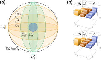
where stands for ‘convex hull’. is the set of fully incoherent states, given by density matrices that are diagonal in the classical basis, while is the set of all states. The intermediate sets obey the strict hierarchy, (see Fig. 1a) and are the free states in the resource theory of multilevel coherence, e.g. is the set of -level coherence-free states.
For a general mixed state one defines the coherence number Chin (2017b, a); Regula et al. (2017), such that a state has a coherence number if and (for consistency, we set ). This parallels the notions of Schmidt number Terhal and Horodecki (2000) and entanglement depth Sørensen and Mølmer (2001) in entanglement theory. A state with coherence number can be decomposed into (at most ) pure states with coherence rank at most , while every such decomposition must contain at least one state with coherence rank at least . A state with is said to exhibit genuine -level coherence, distinguishing it from states that may display coherence between several pairs of levels – potentially even between all such pairs – yet can be prepared as mixtures of pure states with relatively lower-level coherence, see Fig. 1b. In an experiment, the presence of multilevel coherence proves the ability to coherently manipulate a physical system across many of its levels, much in the same way that the creation of states with large entanglement depth provides a certification of the coherent control over several systems.
Note that a state may, at the same time, display large tout-court coherence, but have vanishing higher-level coherence. This is the case, for example, for a superposition of basis elements, like , which does not display -level coherence despite being highly coherent. On the other hand, a pure state may be arbitrarily close to one of the elements of the incoherent basis, yet display non-zero genuine multilevel coherence for all . This is the case, for example, for the state for small . It should be clear that the above multi-level classification provides a much finer description of the coherence properties of quantum systems, but that it is also important to elevate such a finer qualitative classification to a finer quantitative description, as we will do in the following, specifically in Section
Multilevel coherence-free operations and -decohering operations. The second ingredient in the resource theory of multilevel coherence is the set of operations that do not create multilevel coherence. A general quantum operation is described by a linear completely-positive and trace-preserving (CPTP) map, whose action on a state can be written as , in terms of (non-unique) Kraus operators with Nielsen and Chuang (2010). For any map and any set of states, we denote . Generalising the formalism introduced for standard coherence Aberg (2006); Baumgratz et al. (2014); Streltsov et al. (2017), we refer to a CPTP map as a -coherence preserving operation if it cannot increase the coherence level, i.e. . An important subset of these are the -incoherent operations, which are all CPTP maps for which there exists a set of Kraus operators such that for any and all . Note that the (fully) incoherent operations from the resource theory of coherence correspond to . In the Supplementary Material SI we prove that fully incoherent operations are also -incoherent operations for all , and we further define the notion of -decohering maps as those that destroy multilevel coherence: an operation is -decohering if . In particular, we introduce a family of maps that generalize the fully decohering map , which is such that .
Measure of multilevel coherence. The final ingredient for the resource theory of multilevel coherence is a well-defined measure. Very few quantifiers of such a resource have been suggested, and those that exist lack a clear operational interpretation Chin (2017b, a). Furthermore, many of the quantifiers of coherence, such as the intuitive norm of coherence, which measures the off-diagonal contribution to the density matrix, fail to capture the intricate structure of multilevel coherence, as indicated in Fig. 1b. Here we introduce the robustness of multilevel coherence (RMC) as a bona-fide measure that is directly accessible experimentally and efficient to compute for any density matrix. The robustness of -level coherence can be understood as the minimal amount of noise that has to be added to a state to destroy all -level coherence, defined as
| (2) |
This measure generalises the recently introduced robustness of coherence Napoli et al. (2016); Piani et al. (2016) (corresponding to ) to provide full sensitivity to the various levels of multilevel coherence. As a special case of the general notion of robustness of a quantum resource Vidal and Tarrach (1999); Steiner (2003); Piani and Watrous (2015); Geller and Piani (2014); Harrow and Nielsen (2003); Brandao (2005); Brandao and Vianna (2006); Bu et al. (2017), the quantities are known to be valid resource-theoretic measures Horodecki et al. (2009); Streltsov et al. (2017), satisfying non-negativity, convexity, and monotonicity on average with respect to stochastic free operations Vidal and Tarrach (1999); Steiner (2003); Napoli et al. (2016); Piani et al. (2016); Chiribella and Ebler (2016). The latter means for any that for all -incoherent operations with Kraus operators such that and . Since (fully) incoherent operations are -incoherent for any , the RMC also satisfies the strict monotonicity requirement for coherence measures Baumgratz et al. (2014); Streltsov et al. (2017), see Supplementary Material SI .
Crucially, we find that the RMC can be posed as the solution of a semidefinite program (SDP) optimization problem Boyd and Vandenberghe (2004); Vandenberghe and Boyd (1996); Watrous (2013), see Supplementary Material SI . A variety of algorithms exists to solve SDPs efficiently Vandenberghe and Boyd (1996), meaning that the RMC may be computed efficiently for any —in stark contrast to the robustness of entanglement Vidal and Tarrach (1999); Steiner (2003) where one has to deal with the subtleties of the characterisation of the set of separable states Brandao (2005). For an arbitrary -dimensional quantum state we find that
| (3) |
since any such state can be deterministically prepared using only (fully) incoherent operations Baumgratz et al. (2014) starting from the maximally coherent state , for which (see Supplementary Material SI ).
I.2 Experimental verification and quantification of multilevel coherence
We apply our theoretic framework to an experiment that produces four-dimensional quantum states with varying degree and level of coherence using the setup in Fig. 2. We use heralded single photons at a rate of Hz, generated via spontaneous parametric down-conversion in a -Barium borate crystal, pumped by a femto-second pulsed laser at a wavelength of nm. We encode quantum information in the polarisation and path degrees of freedom of these photons to prepare -dimensional systems Ringbauer et al. (2015) with the basis states , where denotes a state of polarisation in mode . This dual-encoding allows for high-precision preparation of arbitrary pure quantum states of any dimension with an average fidelity of and purity of . An arbitrary mixed state can be engineered as a proper mixture, by preparing the states of a pure-state decomposition of for appropriate fractions of the total measurement time and tracing out the classical information about which preparation was implemented. Using the same technique, we can also subject the input states to arbitrary forms of noise.
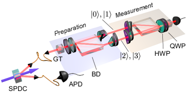
Reversing the preparation stage of the setup allows us to implement arbitrary sharp projective measurements. Arbitrary generalized measurements Nielsen and Chuang (2010) are correspondingly implemented as proper mixtures of a projective decomposition with an average fidelity of . By design, our experiment implements one measurement outcome at a time, which achieves superior precision through the use of a single fibre-coupling assembly Ringbauer et al. (2015), while reducing systematic bias. The whole experiment is characterized by a quantum process fidelity of , limited by the interferometric contrast of . The latter is stable over the relevant timescales of the experiment due to the inherently stable interferometric design with common mode noise rejection for all but the piezo-driven rotational degrees of freedom of the second beam displacer. All data presented here was integrated over s for each outcome, which is also much faster than the observed laser drifts on the order of hours. The main source of statistical uncertainties thus comes from the Poisson-distributed counting statistics. This has been taken into account through Monte-Carlo resampling with runs for tomographic measurements and runs for all other measurements. All experimental data presented in the figures and text throughout the manuscript are based on at least single photon counts and contain 5-equivalent statistical confidence intervals, which are with high confidence normal distributed unless otherwise stated.
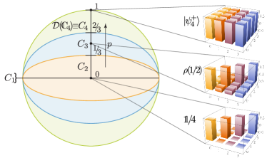
Testbed family of states. To illustrate the phenomenology of multilevel coherence, we consider a family of noisy maximally coherent states
| (4) |
with and finite dimension . These states interpolate between the maximally mixed state (for ) and the maximally coherent state (for ). For this class of states, the RMC can be evaluated analytically to be (see Supplementary Material SI )
| (5) |
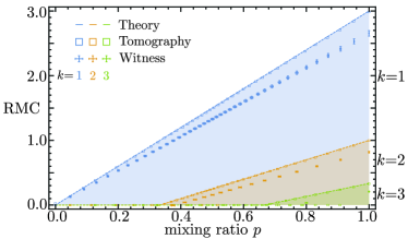
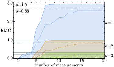
In particular, this implies that for and for , see Supplementary Material SI . The family of noisy maximally coherent states thus provides the ideal testbed for our investigation, spanning the full hierarchy of multilevel coherence, see Fig. 3. Using the setup of Fig. 2 we engineer noisy maximally coherent states for and a variety of values of . We then reconstruct the experimentally prepared states using maximum likelihood quantum state tomography and compute the robustness coherence for all by evaluating the corresponding SDP, Eq. (S13) of the Supplementary Material. As illustrated in Fig. 4, this method produces very reliable results, however, it requires measurements and is thus experimentally infeasible already for medium-scale systems. In the following we introduce and use multilevel-coherence witnesses and other techniques to overcome such a limitation.
I.3 Conditions for genuine multilevel coherence
Given a density matrix , it is immediate to decide whether , as, by definition, this happens if and only if is diagonal. While in Section I.4 we show how one can witness any multilevel coherence through the use of tailored multilevel-coherence witnesses, in this section we focus on simple analytical necessary and sufficient criteria for multilevel coherence. Such criteria also allow us to establish that all sets , for , have non-zero volume within the set of all states.
Necessary and sufficient criteria for coherence beyond two levels. Given a matrix , the associated comparison matrix is defined as (Horn and Johnson, 1994, Definition 2.5.10)
| (6) |
We refer the reader to (Horn and Johnson, 1994, Section 2.5) for more details on the many properties of this construction. We now present our result on the full characterization of the set in arbitrary dimension, whose proof is given the Supplementary Material SI .
Theorem 1.
A density matrix is such that if and only if in the sense of positive semidefiniteness.
An easy corollary of the above result is a simple rule to completely classify qutrit states according to their coherence number. Namely, a qutrit state has coherence number at most if , and otherwise SI .
Necessary conditions for multilevel coherence. As indicated in Fig. 1a, the set of fully incoherent states has zero volume within Piani et al. (2016). This has the important consequence that a state generated randomly will practically never be fully incoherent, and that arbitrarily small perturbations applied to a fully incoherent state will create coherence Ferraro et al. (2010). In other words, under realistic experimental conditions one cannot prepare or verify a fully incoherent state. In contrast, we show in the Supplementary Material SI that the sets are always of non-zero volume for any and thus present a rich, and experimentally meaningful hierarchy within , as shown in Fig. 1a.
Specifically, we have that, if a state satisfies
| (7) |
with the fully decohering map, then . Furthermore, a corollary of Theorem 1 is that if a state satisfies
| (8) |
then such a state cannot have multilevel coherence, i.e. for any reference basis. Observe that the condition (8) is equivalent to being close enough to the maximally mixed state SI , and that the upper bound in Eq. (8) is tight, as it is achieved by states at the boundary of the set of density matrices, e.g., by , with any arbitrary pure state SI . This corollary can be considered the correspondent in coherence theory of the celebrated fact, in entanglement theory, that there is a ball of (fully) separable states surrounding the maximally mixed state Zyczkowski et al. (1998); Gurvits and Barnum (2002, 2003).
I.4 Witnessing multilevel coherence
In analogy with the parallel concept for quantum entanglement, we introduce an efficient alternative to the tomographic approach: multilevel coherence witnesses. In the following we will denote by and the smallest and largest eigenvalues of a Hermitian operator/matrix , respectively.
Since the sets are convex, for any there exists a -level coherence witness such that and for all Rudin (1991). A negative expectation value for thus certifies the -level coherence of in a single measurement.
Given any pure state , one can construct a -level coherence witness as
| (9) |
where are the coefficients rearranged into non-increasing modulus order. This construction ensures that for all with , since SI . On the other hand, it is clear that always reveals the coherence of if present, since , which is negative if . For the maximally coherent state , we then find .
More generally, the set of -level coherence witnesses is obtained as the dual of the set and is characterised by the following theorem, proved in the Supplementary Material SI .
Theorem 2.
A self-adjoint operator is in if and only if
| (10) |
where is the set of all the -element subsets of , and .
Hence, verifying that a given self-adjoint operator is a -level coherence witness requires verifying the positive semidefiniteness of all -dimensional principal sub-matrices of the matrix representation of with respect to the classical basis.
We observe that, while non-trivial multilevel-coherence witnesses necessarily have negative eigenvalues, the number of such negative eigenvalues is severely constrained SI . In particular, we have
Observation 1.
A -level coherence witness has at most negative eigenvalues. All the eigenvalues are bounded from below by .
It is worth remarking that the eigenvector corresponding to the single negative eigenvalue of a -level-coherence witness (that is, ) must exhibit itself -level coherence.
The characterization of multilevel-coherence witnesses of Theorem 2 finds explicit application in the dual form of the SDP formulation of the RMC Boyd and Vandenberghe (2004). In the case of RMC strong duality holds, which means that the primal and dual forms of the problem are equivalent, with the latter given by
| (11) |
Hence, while a lower bound on can be obtained from the negative expectation value of any observable such that , the dual SDP for the RMC actually computes an optimal -level coherence witness whose expectation value matches .
For the family of noisy maximally coherent state , the witness of Eq. (9) turns out to be optimal, independently of the noise parameter , and we calculate . Figure 4 shows the absolute value of the experimentally obtained (negative) expectation values of for a range of values of . This demonstrates that multilevel coherence can be quantitatively witnessed in the laboratory using only a single measurement. Experimentally, however, implementing the optimal witness requires a projection onto a maximally coherent state, which is very sensitive to noise. Indeed, in our experiment we observed a small degree of beam steering by the wave plates, leading to phase uncertainty between the basis states and . As a consequence, the witness becomes suboptimal and only provides a lower bound on the RMC of the experimental state. In contrast, our results show that the larger number of measurements in the tomographic approach and the associated maximum likelihood reconstruction add resilience to experimental imperfections.
I.5 Bounding multilevel coherence
In practice, one might often neither be able to perform full tomography on a system, nor be able to measure the optimal witness. Remarkably, one can obtain a lower bound on the RMC of an experimentally prepared state from any set of experimental data. Specifically, the SDP in Eq. (S16) in the Supplementary Material SI computes the minimal RMC of a state that is consistent with a set of measured expectation values for observables to within experimental uncertainty. This is particularly appealing when one has already performed a set of (well-characterised) measurements and wishes to use these to estimate the multilevel coherence of the input state. Note that linearly independent observables (assuming vanishingly small errors, and not including the identity, which accounts for normalisation) are sufficient to uniquely determine the state, in which case we could use the original SDP, Eq. (11). A similar approach can in principle be used to bound other quantum properties, like entanglement, from limited data Gühne et al. (2007), also via the use of SDPs Eisert et al. (2007). In the case of entanglement one still has to deal with the fact that the separability condition is not a simple SDP constraint, which is relevant even in the case of complete information: so, in general, the obstacle constituted by lack of information, combines with the obstacle of the difficulty of entanglement detection.
We experimentally estimate the lower bounds from Eq. (S16) in the Supplementary Material SI for an increasing number of randomly chosen observables , measured on a -dimensional maximally coherent state and on a noisy maximally coherent state with , see Fig. 5. The results show that our lower bounds become non-trivial already for a small number of observables, and converge to a sub-optimal yet highly informative value. The remaining gap of about between these bounds and the tomographically estimated RMC is due to our conservative error bounds, and could be improved by incorporating maximum-likelihood or Bayesian estimation techniques, see Supplementary Material SI for details. We also find that the number of measurements required for non-trivial bounds increases slowly with the coherence level, and the bounds saturate more quickly for states with more coherence.
We further describe how any single observable may provide a lower bound to the RMC SI . Consider witnesses of the form , with real coefficients, which then give a lower bound to the RMC via Eq. (11). Define the -coherence numerical range of as the interval (the case was studied in Johnson (1981); Johnson and Robinson (1981)), and define its extreme points and . Notice that (similarly for ). Notice also that is the standard numerical range of , and (similarly for the maximal values). In general, for . If , that is, if , then the expectation value of is compatible with being in , and we do not gain any information on . If instead or , the following bound is non-trivial:
| (12) |
Notice that the lower bound is monotonically non-increasing with .
I.6 Multilevel coherence as a resource for quantum-enhanced phase discrimination
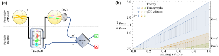
To demonstrate the operational significance of multilevel coherence we show that it is the key resource for the following task, illustrated in Fig. 6a. Suppose that a physical device can apply one of possible quantum operations to a quantum state , according to the known prior probability distribution . The output state is then subject to a single generalized measurement with elements satisfying and . Our objective is to infer the label of the quantum operation that was applied.
We now consider a special case of these tasks, known as phase discrimination, which is an important primitive in quantum information processing, featuring in optimal cloning, dense coding, and error correction protocols Gottesman (1999); Cerf (2000); Hiroshima (2001); Werner (2001). Here the operations imprint a phase on the state through the transformation where is generated by the Hamiltonian . The probability of success for inferring the label in the task specified by is then
| (13) |
Since the Hamiltonian is diagonal in the classical basis and leaves fully incoherent states invariant, the strategy that maximizes while at the same time only making use of incoherent states, is to guess the most likely label, that is, to take , succeeding with probability . On the other hand, a probe state with non-zero coherence can outperform this strategy Napoli et al. (2016); Piani et al. (2016). Here, we find that genuine -level coherence is necessary for to achieve a better than -fold enhancement over in any phase discrimination task .
Theorem 3.
For any phase discrimination task and any probe state ,
| (14) |
This theorem is proved in the Supplementary Material SI , where we also show that for the specific task of discriminating uniformly distributed phases and for a noisy maximally coherent probe, the bound in Eq. (14) becomes tight. This demonstrates the key role of genuine multilevel coherence as a necessary ingredient for quantum-enhanced phase discrimination, unveiling a hierarchical resource structure which goes significantly beyond previous studies only concerned with the coarse-grained description of coherence Piani et al. (2016); Napoli et al. (2016).
Note that this provides an operational significance to the robusteness of multilevel coherence in addition to its operational significance in terms of resilience of noise, which in turn can be thought of also in geometric terms.
Semi-device-independent witnessing of multilevel coherence. An important consequence of Eq. (14) is that whenever , the probe state must have -level coherence. Consequently, the performance of an unknown state in any phase discrimination task provides a witness of genuine multilevel quantum coherence. We remark that the success probability for an arbitrary quantum state can be evaluated without any knowledge of the devices used—neither of the one imprinting the phase, nor the final measurement. Evaluating the witness only relies on the fact that for any , which in turn relies on for any . In other words, under the condition that no information is imprinted on incoherent states, the witness can be evaluated without any additional knowledge of the used devices. We conclude that phase discrimination, as demonstrated in this paper, is a semi-device-independent approach to measure multilevel coherence as quantified by the RMC.
Figure 6 shows our experimental results for semi-device-independent witnessing of multilevel coherence using the phase discrimination task for a range of noisy maximally coherent states, also taking into account experimental imperfections when it comes to the hypothesis for any (see Supplementary Material SI ). As any witnessing approach, this method in general only provides lower bounds on the RMC, yet in contrast to the optimal multilevel witness measured in Fig. 4, the present approach does not rely on any knowledge of the used measurements.
II Discussion
The study of genuine multilevel coherence is pivotal, not only for fundamental questions, but also for applications ranging from transfer phenomena in many-body and complex systems to quantum technologies, including quantum metrology and quantum communication. In particular, for verifying that a quantum device is working in a nonclassical regime it is crucial to certify and quantify multilevel coherence with as few assumptions as possible. Our metrological approach satisfies these criteria by making it possible to verify the preparation of large superpositions and discriminate between them, using only the ability to apply phase transformations that leave incoherent states (approximately) invariant. The goal of the phase-discrimination task we consider is to distinguish a finite-number of phases in a single-shot scenario, and the figure of merit we adopt is the probability of success of correctly identifying the phase imprinted onto the input state. In particular, given our figure of merit, there is no notion of ‘closeness’ of the guess to the actual phase. In contrast, in sensing applications, the task is often to measure an unknown phase with high precision Giovannetti et al. (2011), a task we refer to as ‘phase estimation’. For the latter the figure of merit is the uncertainty of the estimate, and superpositions of the kind , that is, involving eigenstates of the observable that correspond to the largest gap in eigenvalues, can be argued to be optimal Giovannetti et al. (2006). When dealing with phase estimation, the relevant notion is that of unspeakable coherence (or asymmetry) Marvian and Spekkens (2016), and which eigenstates are superposed is very important. On the other hand, for the kind of phase-discrimination task we consider, genuine multilevel coherence of a state like plays a key role. While it was already known that such a maximally coherent state provides the best performance in discriminating equally spaced phases 197 (1976), here we find that the robustness of multilevel coherence of a generic mixed state captures its usefulness in a generic phase discrimination task. This allows us to reverse the argument, and use such usefulness to certify multilevel coherence in a semi-device-independent way.
Our analysis of coherence rank and number, multilevel coherence witnesses, and robustness, uses and adapts notions originally studied in the context of entanglement theory Horodecki et al. (2009), and hence provides further parallels between the resource theories of quantum coherence and entanglement, whose interplay is attracting substantial interest Streltsov et al. (2017). However, a notable difference between the two that we find, emphasise, and exploit, is that multilevel coherence, unlike entanglement, can be characterised and quantified via semidefinite programming, rather than general convex optimisation Brandao (2005). This highlights multilevel coherence as a powerful, yet experimentally accessible quantum resource.
Remarkably, we show that is it possible to use the notion of the comparison matrix to devise a test that faithfully detects genuine three-level coherence and above. We expect such a result to find widespread application in the study of coherence, both theoretically and experimentally. As two immediate applications, we were able to provide a full analytical classification of multilevel coherence for a qutrit, as well as to prove the existence of a ball (actually, the largest possible one, in the Hilbert-Schmidt norm) around the maximally mixed state that contains states that do not exhibit genuine multilevel coherence. This parallels the celebrated result, in entanglement theory, that there is a ball of fully separable states around the maximally mixed state of a multipartite system, and explicitly shows that generating genuine multilevel coherence is a non-trivial experimental task.
It is worth remarking that a number of our results also apply in the case of infinite-dimensional system, such as a harmonic oscillator or quantized field. Indeed, one can always consider, e.g., the quantum (multilevel) coherence exhibited by a system among a subset of states of the incoherent basis, which then provides a bound on the (multilevel) coherence in the entire Hilbert space of the system.
Finally, our work triggers several questions to stimulate further research. These include conceptual questions regarding the exact (geometric) structure and volume of the sets , and how sets and defined with respect to different classical bases intersect, the best further use of tools like the comparison matrix to detect and quantify multilevel coherence, or general purity-based bounds on multilevel coherence. From a more practical point of view, a natural question is how to best choose a finite set of observables to estimate the multilevel coherence of the state of a system, for example via the SDP in the Supplementary Material SI . This is particularly important when one has limited access to the system under observation, as in a biological setting Sarovar et al. (2010); Li et al. (2012); Huelga and Plenio (2013). Independently of the particular choice of observables, our work provides a plethora of readily applicable tools to facilitate the detection, classification, and quantitative estimation of quantum coherence phenomena in systems of potentially large complexity with minimum assumptions, paving the way towards a deeper understanding of their functional role. Further theoretical investigation and experimental progress along these lines may lead to fascinating insights and advances in other branches of science where the detection and exploitation of (multilevel) quantum coherence is or can be of interest.
Acknowledgments
We thank M. B. Plenio, B. Regula, V. Scarani and A. Streltsov for helpful discussions and T. Vulpecula for experimental assistance. This work was supported in part by the Centres for Engineered Quantum Systems (CE110001013) and for Quantum Computation and Communication Technology (CE110001027), the Engineering and Physical Sciences Research Council (grant number EP/N002962/1), and the Templeton World Charity Foundation (TWCF 0064/AB38). We acknowledge financial support from the European Union’s Horizon 2020 Research and Innovation Programme under the Marie Skłodowska-Curie Action OPERACQC (Grant Agreement No. 661338) and the ERC Starting Grant GQCOP (Grant Agreement No. 637352), and from the Foundational Questions Institute under the Physics of the Observer Programme (Grant No. FQXi-RFP-1601).
*
Appendix A SUPPLEMENTARY MATERIAL
Here we provide detailed derivations and proofs of all results in the main text.
A.1 Incoherent and -incoherent operations.
We argue here that a fully incoherent operation is also a -incoherent operation, that is, it cannot create coherence from states that are at most -coherent.
Consider a (fully) incoherent operation with corresponding Kraus operators Baumgratz et al. (2014). This operation is also -incoherent if , where with , for all pure states such that and for all and , which means that the Kraus operators together compose a -incoherent operation. That this holds true is immediate, given that the Kraus operators have the form , with , a phase, and .
A.2 -decohering operations.
We define a -decohering map as one that destroys multilevel coherence, more precisely, such that . These operations generalise the notion of resource destroying maps Liu et al. (2017) to multilevel coherence. An example of a -decohering operation is the -dephasing operation
| (15) |
where is the set of all the -element subsets of , and . Since the are projectors onto -dimensional subspaces, . The linearity and complete positivity of follow directly from the construction. Trace preservation is implied by the observation that has the alternative expression
| (16) |
since is clearly trace-preserving. That Eq. (16) holds can be seen from the fact that, for all with ,
| (17) |
with the number of that contain two fixed indexes. The form of Eq. (16) then follows directly from the definition of in Eq. (15).
A.3 Properties of the sets .
In this section we prove the simple sufficient condition for a state to be in , Eq. (7) of the main text, which also allows us to claim that every with has non-zero volume within the set of all states. We also provide a proof of the characterization of the dual set presented in Theorem 2 of the main text.
Sufficient condition for inclusion in . Using the -dephasing map of Eq. (15) one can characterize a non-zero-volume class of states which are in . Indeed, we argue that any state that satisfies
| (18) |
is in . Let us introduce the set . Such a set is convex. It is also easy to see that, for , such a set has non-zero volume. Indeed, the maximally mixed state satisfies (18) for all , with strict inequality for . This implies that, for any , any state that is an arbitrary but small enough perturbation of the maximally mixed state will still satisfy (18). One has the following.
Theorem 4.
The inclusions hold for any .
Proof of Theorem 4.
For , the inequality characterizes exactly the set of fully incoherent states . This is because, given two normalized states and , implies ; in our case the implication is .
Characterising the dual sets . Here we prove Theorem 2 of the main text, i.e. that if and only if for all .
Proof of Theorem 2.
Formally, the set of -level coherence witnesses is obtained as the dual of the set and given by
| (20) |
This definition, together with the convexity of implies that it is sufficient to see that
| (21) |
if and only if for all . This is immediate since, on the one hand, for any given the action of projecting with on an arbitrary is either to return the null vector or a pure state (up to normalisation) with coherence rank not exceeding . On the other hand, for any such that , one can always find an such that . ∎
A.4 Witness of multilevel coherence for a pure state
In the main text we already argue that the witness
| (22) |
where are the coefficients rearranged in non-increasing modulus order, detects the -multilevel coherence of the state , if present, by means of a negative expectation value . Here we provide details of the proof that is a proper multilevel-cohrence witness, that is, that for all . Given that is a convex set whose extreme points are pure states with coherence rank less or equal to , and given that the trace functional is linear in its argument, it is enough to check that for all pure states with coherence rank less of equal to . Given the structure of , this is equivalent to proving that (actually, with equality). This is readily proven as follows. Let be the decomposition of a generic with , with the -dependent subset of at most coefficients that do not vanish. Then
| (23) |
where: the first inequality is due to the Cauchy-Schwarz inequality; the second inequality comes from the fact that is a normalized state and that we optimize over any index set of cardinality , rather than being restricted to ; the last equality comes from the ordering of the coefficients .
A.5 Eigenvalues of multilevel-coherence witnesses.
As mentioned in Observation 1 in the main text, the number of negative eigenvalues of a multilevel-coherence witness is severely constrained: only if it has at most negative eigenvalues (counting multiplicity). Let also () denote the smallest (largest) eigenvalues of . If , then its most negative eigenvalue, , satisfies
| (24) |
Proof of Observation 1.
Let be the eigenvalues of , ordered in monotonically decreasing order, so that and .
The interlacing theorem Bhatia (2013) states that, if is a Hermitian matrix, and , with a -dimensional projection, then one has , for . In our case , and , for . Since is assumed to be in , , that is, for all . Hence, also the largest eigenvalues of must be non-negative, that is, can at most have negative eigenvalues.
For the proof of Eq. (24), let be the eigenstate corresponding to the lowest eigenvalue of . One has
| (25) |
where the first inequality is due to , and the second inequality follows from the definition of largest and smallest eigenvalue of and the normalization of . In the last inequality, we have used the fact that, for any fixed , it holds (see Section A.4), where are the coefficients of rearranged in non-increasing order, with respect to their modulus. In turn, because of normalization of , and because of the ordering of the coefficients , it holds . Eq. (24) is obtained by simple rearrangement. ∎
It is worth remarking that the -level-coherence witness in Section 1D of the main text saturates the bound on Eq. (24). Also, any optimal multilevel-coherence witness (that is, a witness whose expectation value gives the RMC), has necessarily largest eigenvalue equal to , in order to satisfy tightly the constraint in Eq. (11); thus, any optimal -level-coherence witness actually satisfies .
A.6 Analytical criterion for genuine multilevel coherence
We now present the proof of Theorem 1 in the main text and deduce from it the condition in Eq. (8), which identifies the largest Euclidean ball centered around the maximally mixed state and entirely contained inside . We start by remarking that by Carathéodory’s theorem there exists a decomposition of any density matrix into at most pure states with coherence rank at most . This entails—among other things—that the function is lower semicontinuous, i.e. that if a sequence of density matrices satisfies and then also .
We remind the reader that a matrix is said to be diagonally dominant if (Horn and Johnson, 1990, Definition 6.1.9)
| (26) |
and strictly diagonal dominant if Eq. (26) holds with strict inequality. Diagonally dominant matrices enjoy many useful properties, some of which are as follows.
Lemma 1.
Lemma 2.
As explained in Varga (1976) (see the discussion after Eq. (3.8) there) the above lemma can be deduced from the equivalence of conditions (ii) and (iii) in (Varga, 1976, Theorem 1). In fact, it is not difficult to see that the ‘generalised column diagonal dominance’ condition (iii) is equivalent to the existence of such that is strictly diagonally dominant, while condition (ii) translates directly to because is Hermitian and hence its eigenvalues are automatically real.
Corollary 1.
Given a Hermitian matrix with non-negative diagonal entries, if then also .
Proof.
Another notable corollary is a Hermitian version of a well-known theorem by Camion and Hoffman Camion and Hoffman (1966) (see also (Horn and Johnson, 1994, Theorem 2.5.14)). For a fixed dimension , let us construct the following set of matrices:
| (27) |
Observe that , as one can verify directly by employing Theorem 2 from the main text. In what follows, we will find it convenient to work with Hadamard products (Horn and Johnson, 1990, Definition 7.5.1). We remind the reader that the Hadamard product of two matrices is another matrix whose entries are simply defined by . For a matrix , we set
| (28) |
We now recall the following result. Although it is part of the folklore on the subject, we include a proof for completeness.
Corollary 2.
A Hermitian matrix with non-negative diagonal entries is such that comprises only positive semidefinite matrices if and only if .
Proof.
Since , clearly is necessary to ensure that is composed only of positive semidefinite matrices. To show the converse, observe that for all we have that . By virtue of Corollary 1, it is then clear that is also a sufficient condition. ∎
We are now ready to prove Theorem 1 from the main text, which states that the condition is necessary and sufficient in order for to have coherence number at most .
Proof of Theorem 1.
We start by showing that is sufficient to ensure that . For , set . As in the proof of Corollary 1, we have . Hence, by Lemma 2 there exists such that is strictly diagonally dominant. Since it is easy to see that diagonally dominant density matrices have coherence number at most Johnston et al. (2018), and moreover the coherence number is invariant under congruence by invertible diagonal matrices, we obtain that
Taking the limit and using the fact that is lower semicontinuous we see that in fact also
We now show the converse, i.e. that every density matrix such that satisfies . To this end, we prove that implies that is composed only of positive semidefinite matrices, and then the claim will follow from Corollary 2. If is a decomposition of such that every has coherence rank at most , for all we have
| (29) |
where the last inequality follows because if is nonzero only on a subspace then for some diagonal unitary . ∎
From the above result we can deduce an easy criterion that allows a complete classification of qutrit states based on their coherence number. Notice that it is trivial to check whether , since in the latter case is simply diagonal, so the non-trivial part of the classification is in distinguishing between the case and the case .
Corollary 3.
Let be a qutrit state. If then , otherwise .
Proof.
Since all principal minors of have the same determinant as the corresponding minor of , hence non-negative, Sylverster’s criterion ensures that if and only if . Theorem 1 then ensures that this latter condition is necessary and sufficient in order for to have coherence number at most . ∎
In what follows, we employ Theorem 1 to deduce the condition Eq. (8) of the main text.
Corollary 4.
For all density matrices ,
| (30) |
Proof.
We show that if then necessarily . By Theorem 1, implies that the comparison matrix is not positive semidefinite. Observe that , and moreover . The first equation tells us that since one of the eigenvalues of is negative, the sum of the remaining must be larger than . For fixed , the quantity is well-known to be minimised when for all . Hence, in this case we would obtain . This concludes the proof. ∎
Remark 1.
Observe that the condition on the l.h.s. of (30) is equivalent to the condition
that is, to the condition that is close enough to the maximally mixed state in the Hilbert-Schmidt norm . Indeed, the above result provides the size of the maximal Euclidean ball centered around the maximally mixed state that lies inside the set of -coherent states. There can not be any larger such ball, as the one we constructed already touches the boundary of the set of density matrices. This is because it contains some rank-deficient states, e.g. all normalised projectors onto -dimensional subspaces.
A.7 Robustness of coherence.
It is possible to write as the solution of the following SDP:
| (31) |
The dual SDP is given by Eq. (11) in the main text. We now show that Eq. (31) holds. First, one may rewrite as
| (32) |
One then arrives to Eq. (31) by using the defying property of , that is, that can be written as the convex combination of pure states with coherence rank at most . Thus, for any , we have that if and only if , such that for all it holds that and .
We note that strong duality holds trivially since .
Robustness of multilevel coherence of the noisy maximally coherent states. It is simple to check that for the witness in Eq. (9) in the main text we have and . One then concludes that . On the other hand, it can be seen that for . Then, from Eq. (32) we see that and can hence conclude that
| (33) |
A.8 Bounding RMC from one measurement via witnesses.
For a given observable and corresponding expectation value , we consider witnesses of the form , with real coefficients. The idea is that, since we focus on a subset of all possible witnesses, we will bound the robustness of multilevel coherence exploiting Eq. (11), via
| (34) |
This bound simplifies to
| (35) |
For the convenience of the reader, we restate some of the definitions given in the main text. We define the -coherence numerical range of as the interval , and define its extreme points and . Notice that (similarly for ). Notice also that is the standard numerical range of , and , where is the smallest eigenvalues of (similarly for the maximal values). It is convenient to split the optimization (35) into the two cases and . If we optimize over , the bound assumes the form
| (36) |
while, optimizing over , we have
| (37) |
These two separate optimizations are easily handled. We present the details for the one for ; the one for is handled similarly. For , we want to take as small as possible; at the same time must satisfy
Thus, the optimization is feasible if
Notice that (proven along the lines of Eq. (25)), so that the denominator in the last expression is strictly positive for all as long as is not fully degenerate (in the latter case measuring clearly can not provide any information). If is in the feasible region, we want to take , so that the target value is . If , the largest value is obtained by choosing as negative as possible, that is , so that the optimal value is ; otherwise, if , we take , with optimal value .
Thus, considering also the case , we arrive at the bound of Eq. (12) of the main text:
| (38) |
which is non-trivial when , that is, when the expectation value of is not compatible with being in . Notice that a similar approach is possible in quantifying other resources, like entanglement. One feature that makes multilevel coherence special is that the multilevel-coherence numerical range can be explicitly calculated.
A.9 Bounding RMC from arbitrary measurements.
If one has access to the expectation values of a set of observables measured on an experimentally prepared state , one can lower bound the RMC using the SDP:
| (39) |
where we allow for the lower and upper experimental uncertainties and , respectively. Here we look for an optimal that satisfies while being consistent with the results of the expectation values, that is , within experimental uncertainties.
Note that the SDP in Eq. (39) only requires the optimization to reproduce the measured expectation values to within the supplied error bounds. This leads to a trade-off, where smaller error bounds to the SDP lead to closer convergence to the actual value of multilevel coherence, while larger error bounds improve the stability of the estimation against statistical fluctuations. In the experiment presented in Fig. 5 of the main text, we have chosen conservative error bounds, leading to a deviation about between the lower bound and the tomographically estimated RMC. This could be improved by incorporating maximum-likelihood or Bayesian estimation techniques as in the case of quantum tomography.
A.10 Phase discrimination.
Consider the optimal satisfying the optimisation in Eq. (32) for a given state , i.e. such that . Following from the linearity of the success probability in Eq. (13) in the main text, we see that
| (40) |
Now, by setting , one may also consider the optimal such that , which means
| (41) |
Overall then, we have
| (42) |
Since , we find that . Furthermore, we have already seen that . Hence, we arrive at
| (43) |
which can be rearranged to Eq. (14) in the main text.
When one considers the phase discrimination task with a probe prepared in the noisy maximally coherent state and optimised generalised measurements , the success probability is Napoli et al. (2016); Piani et al. (2016)
| (44) |
This can be input into the lower bound to in Eq. (14) in the main text, for which we see that
| (45) |
In fact, it can be seen from Eq. (33) that this lower bound is tight.
A.11 Experimental Imperfections
Recall, that the phase discrimination task witnesses the robustness of multilevel coherence in a quasi-device independent way, relying only on the mild assumption that the device leaves incoherent states unperturbed. In practice, this assumption is not exactly satisfied, since experimental imperfections in general lead to unitaries that do not leave incoherent states exectly invariant. To take this into account, we replacing the upper bound on the incoherent success probability with an upper bound for the probability of success for discriminating the elements of the ensemble , where by we denote the image of a incoherent state under the action of a map which describes the approximate application of a phase .
In general, given an ensemble of possible states in which a system may be prepared, the optimal probability of guessing the actual state is given by , with the classical-quantum state Konig et al. (2009). In our case . We will assume that the maps do not modify an incoherent state too much; more precisely, in terms of trace distance , for all . This means that , with and , which in turn implies that . It is immediate to check that then , with a normalized state. This proves that . We can give a reasonable estimate of in terms of the process fidelity of the experiment, using the Fuchs-van de Graaf inequality , with the fidelity between two states Fuchs and van de Graaf (1999). Thus, we arrive at the estimate , which can be substituted in place of in Eq. (14) in the main text. In the case of our experiment with process fidelity and , this means substituting with .
References
- Streltsov et al. (2017) A. Streltsov, G. Adesso, and M. B. Plenio, “Colloquium: Quantum coherence as a resource,” Rev. Mod. Phys. 89, 041003 (2017).
- Aberg (2006) J. Aberg, “Quantifying superposition,” arXiv preprint quant-ph/0612146 (2006).
- Baumgratz et al. (2014) T. Baumgratz, M. Cramer, and M. Plenio, “Quantifying coherence,” Phys. Rev. Lett. 113, 140401 (2014).
- Marvian and Spekkens (2016) I. Marvian and R. W. Spekkens, “How to quantify coherence: distinguishing speakable and unspeakable notions,” Phys. Rev. A 94, 052324 (2016).
- Coecke et al. (2016) B. Coecke, T. Fritz, and R. W. Spekkens, “A mathematical theory of resources,” Inf. Comp. 250, 59 (2016).
- Horodecki and Oppenheim (2013) M. Horodecki and J. Oppenheim, “(Quantumness in the context of) resource theories,” Intl. J. Mod. Phys. B 27, 1345019 (2013).
- Brandão and Gour (2015) F. G. Brandão and G. Gour, “Reversible framework for quantum resource theories,” Phys. Rev. Lett. 115, 070503 (2015).
- Napoli et al. (2016) C. Napoli, T. R. Bromley, M. Cianciaruso, M. Piani, N. Johnston, and G. Adesso, “Robustness of Coherence: An Operational and Observable Measure of Quantum Coherence,” Phys. Rev. Lett. 116, 150502 (2016).
- Piani et al. (2016) M. Piani, M. Cianciaruso, T. R. Bromley, C. Napoli, N. Johnston, and G. Adesso, “Robustness of asymmetry and coherence of quantum states,” Phys. Rev. A 93, 042107 (2016).
- Yuan et al. (2015) X. Yuan, H. Zhou, Z. Cao, and X. Ma, “Intrinsic randomness as a measure of quantum coherence,” Phys. Rev. A 92, 022124 (2015).
- Winter and Yang (2016) A. Winter and D. Yang, “Operational resource theory of coherence,” Phys. Rev. Lett. 116, 120404 (2016).
- Biswas et al. (2017) T. Biswas, M. García Díaz, and A. Winter, “Interferometric visibility and coherence,” Proc. Royal Soc. A 473, 20170170 (2017).
- Streltsov et al. (2015) A. Streltsov, U. Singh, H. S. Dhar, M. N. Bera, and G. Adesso, “Measuring quantum coherence with entanglement,” Phys. Rev. Lett. 115, 020403 (2015).
- Chitambar et al. (2016) E. Chitambar, A. Streltsov, S. Rana, M. Bera, G. Adesso, and M. Lewenstein, “Assisted distillation of quantum coherence,” Phys. Rev. Lett. 116, 070402 (2016).
- Adesso et al. (2016) G. Adesso, T. R. Bromley, and M. Cianciaruso, “Measures and applications of quantum correlations,” J. Phys. A 49, 473001 (2016).
- Marvian et al. (2016) I. Marvian, R. W. Spekkens, and P. Zanardi, “Quantum speed limits, coherence, and asymmetry,” Phys. Rev. A 93, 052331 (2016).
- Girolami (2014) D. Girolami, “Observable measure of quantum coherence in finite dimensional systems,” Phys. Rev. Lett. 113, 170401 (2014).
- Ren et al. (2017) H. Ren, A. Lin, S. He, and X. Hu, “Quantitative coherence witness for finite dimensional states,” Ann. Phys. 387, 281 (2017).
- Kammerlander and Anders (2016) P. Kammerlander and J. Anders, Sci. Rep. 6, 22174 (2016).
- Uzdin et al. (2015) R. Uzdin, A. Levy, and R. Kosloff, “Equivalence of quantum heat machines, and quantum-thermodynamic signatures,” Phys. Rev. X 5, 031044 (2015).
- Hillery (2016) M. Hillery, “Coherence as a resource in decision problems: The deutsch-jozsa algorithm and a variation,” Phys. Rev. A 93, 012111 (2016).
- Giorda and Allegra (2018) P. Giorda and M. Allegra, “Coherence in quantum estimation,” J. Phys. A 51, 025302 (2018).
- Zhang et al. (2017) C. Zhang, B. Yadin, Z.-B. Hou, H. Cao, B.-H. Liu, Y.-F. Huang, R. Maity, V. Vedral, C.-F. Li, G.-C. Guo, and D. Girolami, “Detecting metrologically useful asymmetry and entanglement by a few local measurements,” Phys. Rev. A 96, 042327 (2017).
- Braun et al. (2017) D. Braun, G. Adesso, F. Benatti, R. Floreanini, U. Marzolino, M. W. Mitchell, and S. Pirandola, “Quantum enhanced measurements without entanglement,” arXiv preprint arXiv:1701.05152 (2017).
- Levi and Mintert (2014) F. Levi and F. Mintert, “A quantitative theory of coherent delocalization,” New J. Phys. 16, 033007 (2014).
- Sperling and Vogel (2015) J. Sperling and W. Vogel, “Convex ordering and quantification of quantumness,” Physica Scripta 90, 074024 (2015).
- Killoran et al. (2016) N. Killoran, F. E. Steinhoff, and M. B. Plenio, “Converting nonclassicality into entanglement,” Phys. Rev. Lett. 116, 080402 (2016).
- Horodecki et al. (2009) R. Horodecki, P. Horodecki, M. Horodecki, and K. Horodecki, “Quantum entanglement,” Rev. Mod. Phys. 81, 865 (2009).
- Gühne and Tóth (2009) O. Gühne and G. Tóth, “Entanglement detection,” Phys. Rep. 474, 1 (2009).
- Li et al. (2012) C.-M. Li, N. Lambert, Y.-N. Chen, G.-Y. Chen, and F. Nori, “Witnessing quantum coherence: from solid-state to biological systems,” Sci. Rep. 2, 885 (2012).
- Lostaglio et al. (2015) M. Lostaglio, D. Jennings, and T. Rudolph, “Description of quantum coherence in thermodynamic processes requires constraints beyond free energy,” Nat. Commun. 6, 6383 (2015).
- Scholes et al. (2017) G. D. Scholes, G. R. Fleming, L. X. Chen, A. Aspuru-Guzik, A. Buchleitner, D. F. Coker, G. S. Engel, R. van Grondelle, A. Ishizaki, D. M. Jonas, J. S. Lundeen, J. K. McCusker, S. Mukamel, J. P. Ogilvie, A. Olaya-Castro, M. A. Ratner, F. C. Spano, K. B. Whaley, and X. Zhu, “Using coherence to enhance function in chemical and biophysical systems,” Nature 543, 647 (2017).
- Witt and Mintert (2013) B. Witt and F. Mintert, “Stationary quantum coherence and transport in disordered networks,” New J. Phys. 15, 093020 (2013).
- Scholak et al. (2011) T. Scholak, F. de Melo, T. Wellens, F. Mintert, and A. Buchleitner, “Efficient and coherent excitation transfer across disordered molecular networks,” Phys. Rev. E 83, 021912 (2011).
- Tiersch et al. (2012) M. Tiersch, S. Popescu, and H. J. Briegel, “A critical view on transport and entanglement in models of photosynthesis,” Phil. Trans. Royal Soc. London A 370, 3771 (2012).
- Chin (2017a) S. Chin, “Generalized coherence concurrence and path distinguishability,” J. Phys. A 50, 475302 (2017a).
- Regula et al. (2017) B. Regula, M. Piani, M. Cianciaruso, T. R. Bromley, A. Streltsov, and G. Adesso, “Converting multilevel nonclassicality into genuine multipartite entanglement,” arXiv preprint arXiv:1704.04153 (2017).
- Chin (2017b) S. Chin, “Coherence number as a discrete quantum resource,” Phys. Rev. A 96, 042336 (2017b).
- Gottesman (1999) D. Gottesman, “Fault-tolerant quantum computation with higher-dimensional systems,” in Quantum Computing and Quantum Communications (Springer, 1999) pp. 302–313.
- Barnett and Croke (2009) S. M. Barnett and S. Croke, “Quantum state discrimination,” Adv. Opt. Photon. 1, 238 (2009).
- (41) See Supplementary Material for details on the derivations and proofs.
- Terhal and Horodecki (2000) B. M. Terhal and P. Horodecki, “Schmidt number for density matrices,” Phys. Rev. A 61, 040301 (2000).
- Sørensen and Mølmer (2001) A. S. Sørensen and K. Mølmer, “Entanglement and extreme spin squeezing,” Phys. Rev. Lett. 86, 4431 (2001).
- Nielsen and Chuang (2010) M. Nielsen and I. Chuang, Quantum Computation and Quantum Information (Cambridge University Press, 2010).
- Vidal and Tarrach (1999) G. Vidal and R. Tarrach, “Robustness of entanglement,” Phys. Rev. A 59, 141 (1999).
- Steiner (2003) M. Steiner, “Generalized robustness of entanglement,” Phys. Rev. A 67, 054305 (2003).
- Piani and Watrous (2015) M. Piani and J. Watrous, “Necessary and sufficient quantum information characterization of einstein-podolsky-rosen steering,” Phys. Rev. Lett. 114, 060404 (2015).
- Geller and Piani (2014) J. Geller and M. Piani, “Quantifying non-classical and beyond-quantum correlations in the unified operator formalism,” J. Phys. A 47, 424030 (2014).
- Harrow and Nielsen (2003) A. W. Harrow and M. A. Nielsen, “Robustness of quantum gates in the presence of noise,” Phys. Rev. A 68, 012308 (2003).
- Brandao (2005) F. G. Brandao, “Quantifying entanglement with witness operators,” Phys. Rev. A 72, 022310 (2005).
- Brandao and Vianna (2006) F. G. Brandao and R. O. Vianna, “Witnessed entanglement,” Intl. J. Quant. Info. 4, 331 (2006).
- Bu et al. (2017) K. Bu, N. Anand, and U. Singh, “Asymmetry and coherence weight of quantum states,” arXiv preprint arXiv:1703.01266 (2017).
- Chiribella and Ebler (2016) G. Chiribella and D. Ebler, “Optimal quantum networks and one-shot entropies,” New J. Phys. 18, 093053 (2016).
- Boyd and Vandenberghe (2004) S. Boyd and L. Vandenberghe, Convex optimization (Cambridge university press, 2004).
- Vandenberghe and Boyd (1996) L. Vandenberghe and S. Boyd, “Semidefinite programming,” SIAM review 38, 49 (1996).
- Watrous (2013) J. Watrous, “Simpler semidefinite programs for completely bounded norms,” Chicago Journal of Theoretical Computer Science 2013 (2013).
- Ringbauer et al. (2015) M. Ringbauer, B. Duffus, C. Branciard, E. G. Cavalcanti, A. G. White, and A. Fedrizzi, “Measurements on the reality of the wavefunction,” Nat. Phys. 11, 249 (2015).
- Horn and Johnson (1994) R. A. Horn and C. R. Johnson, Topics in Matrix Analysis, Topics in Matrix Analysis (Cambridge University Press, 1994).
- Ferraro et al. (2010) A. Ferraro, L. Aolita, D. Cavalcanti, F. Cucchietti, and A. Acin, “Almost all quantum states have nonclassical correlations,” Phys. Rev. A 81, 052318 (2010).
- Zyczkowski et al. (1998) K. Zyczkowski, P. Horodecki, A. Sanpera, and M. Lewenstein, “Volume of the set of separable states,” Phys. Rev. A 58, 883 (1998).
- Gurvits and Barnum (2002) L. Gurvits and H. Barnum, “Largest separable balls around the maximally mixed bipartite quantum state,” Phys. Rev. A 66, 062311 (2002).
- Gurvits and Barnum (2003) L. Gurvits and H. Barnum, “Separable balls around the maximally mixed multipartite quantum states,” Phys. Rev. A 68, 042312 (2003).
- Rudin (1991) W. Rudin, Functional analysis (Tata McGraw-Hill, 1991).
- Gühne et al. (2007) O. Gühne, M. Reimpell, and R. F. Werner, “Estimating entanglement measures in experiments,” Phys. Rev. Lett. 98, 110502 (2007).
- Eisert et al. (2007) J. Eisert, F. G. S. L. Brandão, and K. M. R. Audenaert, “Quantitative entanglement witnesses,” New Journal of Physics 9, 46 (2007).
- Johnson (1981) C. R. Johnson, “Numerical ranges of principal submatrices,” Linear Algebra and its Applications 37, 23 (1981).
- Johnson and Robinson (1981) C. R. Johnson and H. A. Robinson, “Eigenvalue inequalities for principal submatrices,” Linear Algebra and its Applications 37, 11 (1981).
- Cerf (2000) N. J. Cerf, “Asymmetric quantum cloning in any dimension,” J. Mod. Opt. 47, 187 (2000).
- Hiroshima (2001) T. Hiroshima, “Optimal dense coding with mixed state entanglement,” J. Phys. A 34, 6907 (2001).
- Werner (2001) R. F. Werner, “All teleportation and dense coding schemes,” J. Phys. A 34, 7081 (2001).
- Giovannetti et al. (2011) V. Giovannetti, S. Lloyd, and L. Maccone, “Advances in quantum metrology,” Nat. Photon. 5, 222 (2011).
- Giovannetti et al. (2006) V. Giovannetti, S. Lloyd, and L. Maccone, “Quantum metrology,” Phys. Rev. Lett. 96, 010401 (2006).
- 197 (1976) Quantum Detection and Estimation Theory, Mathematics in Science and Engineering (Elsevier Science, 1976).
- Sarovar et al. (2010) M. Sarovar, A. Ishizaki, G. R. Fleming, and K. B. Whaley, “Quantum entanglement in photosynthetic light-harvesting complexes,” Nat. Phys. 6, 462 (2010).
- Huelga and Plenio (2013) S. F. Huelga and M. B. Plenio, “Vibrations, quanta and biology,” Contemp. Phys. 54, 181 (2013).
- Liu et al. (2017) Z.-W. Liu, X. Hu, and S. Lloyd, “Resource destroying maps,” Phys. Rev. Lett. 118, 060502 (2017).
- Bhatia (2013) R. Bhatia, Matrix analysis, Vol. 169 (Springer Science & Business Media, 2013).
- Horn and Johnson (1990) R. A. Horn and C. R. Johnson, Matrix Analysis (Cambridge University Press, 1990).
- Varga (1976) R. S. Varga, “On recurring theorems on diagonal dominance,” Linear Algebra Appl. 13, 1 (1976).
- Camion and Hoffman (1966) P. Camion and A. J. Hoffman, “On the nonsingularity of complex matrices,” Pacific J. Math. 17, 211 (1966).
- Johnston et al. (2018) N. Johnston, C.-K. Li, S. Plosker, and Y.-T. Poon, “Some notes on the robustness of -coherence,” Preprint arXiv:1806.00653 (2018).
- Konig et al. (2009) R. Konig, R. Renner, and C. Schaffner, “The operational meaning of min- and max-entropy,” IEEE Trans. Inf. Theory 55, 4337 (2009).
- Fuchs and van de Graaf (1999) C. A. Fuchs and J. van de Graaf, “Cryptographic distinguishability measures for quantum-mechanical states,” IEEE Trans. Inf. Theory 45, 1216 (1999).