Critical exponent $\omega$ in the Gross-Neveu-Yukawa model at $O(1/N)$

Abstract. The critcal exponent $\omega$ is evaluated at $O(1/N)$ in $d$-dimensions in the Gross-Neveu model using the large $N$ critical point formalism. It is shown to be in agreement with the recently determined three loop $\beta$-functions of the Gross-Neveu-Yukawa model in four dimensions. The same exponent is computed for the chiral Gross-Neveu and non-abelian Nambu-Jona-Lasinio universality classes.

LTH 1138

1 Introduction.

The Gross-Neveu (GN) model is a remarkably simple quantum field theory of a fermion field with a quartic interaction but which has a rich spectrum of properties with applications to many areas of physics. It was first studied at length in the particle physics context in [1] but was introduced in [2] and is also known as the Ashkin-Teller model. In [1] it was shown that the theory was renormalizable in two dimensions and is asymptotically free. When the model is endowed with an $O(N)$ or $SU(N)$ symmetry it can be solved within the large $N$ expansion, [1], where it is apparent that there is dynamical symmetry breaking. The originally massless fermion field becomes massive in the true non-perturbative vacuum and contains a massive $2$-fermion bound state particle in the spectrum. In many ways the Gross-Neveu model features a large cross-section of properties of some four dimensional gauge theories such as Quantum Chromodynamics (QCD) which means it is a simpler forum for testing out ideas in higher dimensional quantum field theories. Unlike gauge theories the exact $S$-matrix can be written down for the Gross-Neveu model, [3], from which the full spectrum of bound states can be deduced. Also the exact mass gap which fixes the scale of the dynamically generated mass has been computed from the exact $S$-matrix, [4]. In terms of other connections to physics, the Gross-Neveu model critical exponents derived from the renormalization group functions at the $d$-dimensional Wilson-Fisher fixed point for a particular value of $N$ have recently been shown to describe the critical dynamics of a phase transition in graphene, [5]. This rather novel and perhaps surprising connection may offer a hope that the Gross-Neveu model, which is sometimes used as a theoretical laboratory for a four dimensional gauge theory, could in fact become an experimental one. For instance, it has been suggested in [5] that the transition in graphene could be a paradigm of Standard Model spontaneous symmetry breaking.

There is also perhaps more immediate interest in the Gross-Neveu model due to recent connections with other four dimensional theories as well as AdS/CFT ideas, [6, 7, 8]. For instance, the model is one of a set of theories which resides in the infinite tower of quantum field theories at the $d$-dimensional Wilson-Fisher fixed point. Another constituent of this universality class is the Gross-Neveu-Yukawa theory (GNY) which is renormalizable in four dimensions with the connection to the Gross-Neveu model being illuminated in [9]. For instance, both have the same core boson-fermion interaction differing only in the purely bosonic sector which is present to ensure renormalizability in their respective critical dimensions. The current term for such a connection is ultraviolet completion which has opened up interesting ideas for aspects of the Standard Model. For instance, a $4$-fermi interaction is non-renormalizable in four dimensions but by contrast the Gross-Neveu-Yukawa theory is renormalizable. The former was used as an effective theory in the early years of trying to understand weak interactions prior to the discovery of mass generation via spontaneous symmetry breaking and the Higgs mechanism. Within the Gross-Neveu-Yukawa model there is a bosonic field which is parallel to the Higgs field in that it also has a quartic self-interaction. More recently it has been shown that for a low value of $N$ when there is an $SU(N)$ symmetry the theory has an emergent supersymmetry, [7]. By this it is meant that when the fixed point spectrum is determined from the zeros of the two $\beta$-functions, there is one solution where the coupling constants are equal and moreover the anomalous dimensions of the fields evaluated at that fixed point are equal. This offers an interesting possibility of exploring a new way of going beyond the Standard Model. As such the Gross-Neveu-Yukawa model is an excellent forum to explore such new ideas. Necessary to achieve this at high precision is knowledge of the renormalization group functions at high loop order. Recently the three loop renormalization group functions of the Gross-Neveu-Yukawa model were computed in the $\overline{\mbox{MS}}$ (modified minimal subtraction) scheme, [10], which extended the two loop results of [11]. Given recent advances in multiloop techniques it would be reasonable to expect four loop results in the near future. Aside from the graphene connection through the Gross-Neveu universality class, such high order loop computations are required if one is to extend the Standard Model renormalization group functions to the same precision.

One aspect which naturally arises in this context is the need to have checks on such intensely complicated computations at four loops. This is provided for via the critical point large $N$ expansion which was developed originally for the $O(N)$ $\phi^{4}$ theory or equivalently the Ising model universality class in [12, 13, 14]. There the first three terms of the $d$-dimensional large $N$ critical exponents were determined and these contain information on the renormalization group functions of all the theories lying in the same universality class. In particular expanding the exponents in powers of $\epsilon$ where the spacetime dimension $d$ is set to $d$ $=$ $D$ $-$ $2\epsilon$ where $D$ is the critical dimension of a theory, there is a one-to-one correspondence with the $\epsilon$ expansion of the renormalization group functions at that theory’s Wilson-Fisher fixed point. So the $d$-dimensional large $N$ critical exponents contain information on parts of the renormalization group functions which have not yet been computed explicitly. If several orders in $1/N$ are available such information is a useful independent blind test of any new loop order evaluation. The method used to determine the large $N$ critical exponents of the Ising model universal theory has been extended to the Gross-Neveu universality class as well as related classes involving a simple core boson-fermion Yukawa type interaction, [15, 16, 17, 18, 19, 20, 21]. These exponents have proved useful in comparing with explicit Gross-Neveu perturbative computations. However, in order to extract new information for the four dimensional Gross-Neveu-Yukawa theory from these results beyond what is currently available in perturbation theory one key large $N$ critical exponent has yet to be determined which is denoted by $\omega$. It relates to the $\beta$-function slope at criticality relative to the four dimensional theory and it is the purpose of this article to compute it at leading order in large $N$. This is not only for the Gross-Neveu universality class, which contains the Gross-Neveu-Yukawa theory, but also for the chiral Gross-Neveu and non-abelian Nambu-Jona-Lasinio universality classes. The reason why these other classes are considered is that they are endowed with a combination of symmetries different from the Gross-Neveu class such as continuous chiral symmetry with fermions lying in multiplets of non-abelian groups. As such they are closer to the symmetries of the Standard Model. Aside from this connection to Standard Model renormalization group functions knowledge of $\omega$ will add to the information which is accumulating on our understanding of ultraviolet completeness and $d$-dimensional conformal field theories.

The article is organized as follows. The large $N$ critical point formalism of [12, 13] extended to the Gross-Neveu model in [15] is reviewed in section $2$ in the context of evaluating $\omega$ at $O(1/N)$. The explicit equations from which $\omega$ is determined at this order are constructed in section $3$ where an underlying two loop large $N$ graph which is required is evaluated using massless coordinate space techniques. The main result for $\omega$ at $O(1/N)$ is given here and its $\epsilon$ expansion reconciled with the four dimensional renormalization group functions. The formalism of these two sections is extended in the subsequent section to the other two $4$-fermi universality classes and $\omega$ is deduced for each. Finally, we provide conclusions in section $5$.

2 Formalism.

We begin by recalling the relevant aspects of the Gross-Neveu and Gross-Neveu-Yukawa models and the large $N$ formalism in order to be able to compute the critical exponent $\omega$ at $O(1/N)$. First, the respective Lagrangians are, [1],

$$L_{\mbox{\footnotesize{GN}}}~{}=~{}i\bar{\psi}^{i}\partial\!\!\!/\psi^{i}~{}+~{}\frac{1}{2}g\sigma\bar{\psi}^{i}\psi^{i}~{}-~{}\frac{1}{2}\sigma^{2}$$ (2.1)

for the two dimensional Gross-Neveu (GN) model where $1$ $\leq$ $i$ $\leq$ $N$, and, [9],

$$L_{\mbox{\footnotesize{GNY}}}~{}=~{}i\bar{\psi}^{i}\partial\!\!\!/\psi^{i}~{}+~{}\frac{1}{2}\partial_{\mu}\sigma\partial^{\mu}\sigma~{}+~{}\frac{1}{2}g_{1}\sigma\bar{\psi}^{i}\psi^{i}~{}+~{}\frac{1}{24}g_{2}^{2}\sigma^{4}$$ (2.2)

for the four dimensional Gross-Neveu-Yukawa (GNY) model. In both cases the fermion field $\psi^{i}$ has an $SU(N)$ symmetry with $1$ $\leq$ $i$ $\leq$ $N$ and $\sigma$ is a bosonic field. In (2.1) this field is actually an auxiliary and it can be eliminated to produce the Lagrangian, [1],

$$L_{\mbox{\footnotesize{GN}}}~{}=~{}i\bar{\psi}^{i}\partial\!\!\!/\psi^{i}~{}+~{}\frac{1}{2}g^{2}(\bar{\psi}^{i}\psi^{i})^{2}$$ (2.3)

which is asymptotically free and renormalizable in two dimensions, [1]. By contrast in (2.2) $\sigma$ has a canonical kinetic term and hence it cannot be eliminated from the Lagrangian which is renormalizable in four dimensions. Both Lagrangians share common properties. The coupling constants of each theory are dimensionless in the respective critical dimensions which means that the canonical dimension of $\sigma$ is the same in both Lagrangians. This is not an accident since the Gross-Neveu-Yukawa model is the ultraviolet completion of (2.1) and both are contained within the same universality class at their respective Wilson-Fisher fixed points. In addition both (2.1) and (2.2) have one interaction the same which we will term the core interaction and which is the fundamental interaction of the underlying universality class at the respective Wilson-Fisher fixed points. While the canonical dimension of the fermion is different in the critical dimensions of each Lagrangian it can be expressed as $\mbox{\small{$\frac{1}{2}$}}(d-1)$ where $d$ is the spacetime dimension. Thus the $4$-fermi interaction of (2.3) would be a dimension six operator if it was present in (2.2) and hence would correspond to a non-renormalizable operator. In noting that both theories have a connection through the ultraviolet completion it has been known for a long time that both can be studied via the large $N$ expansion where $1/N$ is regarded as a small perturbative parameter, [1, 9]. As $1/N$ is a dimensionless parameter it turns out that one can obtain information about the underlying universality class which contains both (2.1) and (2.2). In particular it is possible to compute the critical exponents of the universal theory order by order in $1/N$ in an arbitrary spacetime dimension $d$ and moreover to three orders in $1/N$. This was first carried out for the $O(N)$ nonlinear $\sigma$ model and $\phi^{4}$ theory in [12, 13, 14]. Thereafter the same information was determined for the $O(N)$ Gross-Neveu universality class in [15, 16, 17, 18, 19, 20, 21]. These critical exponents contain all the information on the renormalization group functions in the tower of theories lying along a Wilson-Fisher fixed point in $d$-dimensions. For instance, expanding the exponents in $d$ $=$ $2$ $-$ $2\epsilon$ or $d$ $=$ $4$ $-$ $2\epsilon$ one obtains the $\epsilon$ expansion of the critical exponents derived from the respective renormalization group functions of (2.1) and (2.2). For the latter case we now focus on computing $\omega$ at $O(1/N)$ in order to obtain information on the Gross-Neveu-Yukawa renormalization group functions.

The first stage is to write down the universal Lagrangian used for the large $N$ formalism which is

$$L_{\mbox{\footnotesize{GN}}}~{}=~{}i\bar{\psi}^{i}\partial\!\!\!/\psi^{i}~{}+~{}\frac{1}{2}\tilde{\sigma}\bar{\psi}^{i}\psi^{i}~{}-~{}\frac{1}{2g^{2}}\tilde{\sigma}^{2}~{}.$$ (2.4)

The only difference between (2.1) and (2.4) is that the coupling constant has been rescaled out of the core interaction which will be the only interaction relevant in the universal theory. In (2.2), for instance, the quartic $\sigma$ interaction, which is akin to the Higgs interaction in the Standard Model, is included with the core interaction to ensure the field theory is renormalizable in the critical dimension of $4$. By contrast in the universal theory (2.4) such an interaction emerges naturally through box graphs with four external $\sigma$ legs and only the $\sigma\bar{\psi}^{i}\psi^{i}$ interaction. Such a property was first noted in [22] for the critical point equivalence of the non-abelian Thirring model and QCD in the large $N_{\!f}$ expansion where $N_{\!f}$ is the number of (massless) quark flavours as opposed to an expansion in $1/N_{\!c}$ where $N_{\!c}$ is the number of colours. The final term of (2.4) is only included to make the connection with (2.1) and is not central to setting up the $1/N$ formalism developed in [12, 13]. It is actually the first two terms of (2.4) which define the scaling behaviour of the fields at criticality. From these we can define the respective full dimensions of the $\psi^{i}$ and $\sigma$ fields as, [15],

$$\alpha~{}=~{}\mu~{}+~{}\mbox{\small{$\frac{1}{2}$}}\eta~{}~{}~{},~{}~{}~{}\beta~{}=~{}1~{}-~{}\eta~{}-~{}\chi$$ (2.5)

where $d$ $=$ $2\mu$ for shorthand, $\eta$ is the anomalous dimension exponent of the $\psi^{i}$ field and $\chi$ is the exponent associated with the anomalous dimension of the core interaction. Once these dimensions are specified then the asymptotic scaling forms of the respective propagators in the approach to criticality can be specified as

$$\psi(x)~{}\sim~{}\frac{Ax\!\!\!/}{(x^{2})^{\alpha}}~{}~{}~{},~{}~{}~{}\sigma(x)~{}\sim~{}\frac{B}{(x^{2})^{\beta}}$$ (2.6)

in coordinate space where we use the same letter as the field to denote the propagator. The canonical part of $\alpha$ is not inconsistent with the canonical dimension of $\psi^{i}$ due to the presence of $x\!\!\!/$ in the numerator of the scaling form of the propagator. Also $A$ and $B$ are $x$-independent amplitudes which always appear within computations in the combination $z$ $=$ $A^{2}B$. We will work in coordinate space throughout and use the same notation as [15]. We recall that the $1/N$ expansion of various quantities will be written as

$$\eta~{}=~{}\sum_{n=1}^{\infty}\frac{\eta_{n}}{N^{n}}~{}~{}~{},~{}~{}~{}z~{}=~{}\sum_{n=1}^{\infty}\frac{z_{n}}{N^{n}}$$ (2.7)

for example. As these and other quantities have already been computed in the Gross-Neveu universality class we recall the various $O(1/N)$ expressions here for completeness. We have, [15, 17, 18],

$$\eta_{1}~{}=~{}-~{}\frac{2(\mu-1)\Gamma(2\mu-1)}{\mu\Gamma^{3}(\mu)\Gamma(1-\mu)}~{}~{}~{},~{}~{}~{}\chi_{1}~{}=~{}\frac{\mu\eta_{1}}{(\mu-1)}~{}~{}~{},~{}~{}~{}z_{1}~{}=~{}\frac{1}{2}\Gamma^{2}(\mu)\eta_{1}$$ (2.8)

where we note that throughout we take the spinor trace convention as $\mbox{tr}I$ $=$ $2$. While this is consistent when comparing with two dimensional perturbation theory in order to compare any exponent with the critical exponents derived from four dimensional renormalization group functions one replaces $N$ by $2N$. This is because within Feynman graphs a factor of $N$ is always associated with a closed fermion loop. The exponents of (2.8) were determined by solving the skeleton Schwinger-Dyson equations for the two $2$-point functions order by order at criticality using the asymptotic scaling forms (2.6), [15, 17, 18].

The procedure to determine $\omega$ at $O(1/N)$ follows the same route as that to find $\eta_{1}$ except that the leading asymptotic scaling forms of the propagators are extended to

$$\psi(x)~{}\sim~{}\frac{Ax\!\!\!/}{(x^{2})^{\alpha}}\left[1+A^{\prime}(x^{2})^{\omega}\right]~{}~{}~{},~{}~{}~{}\sigma(x)~{}\sim~{}\frac{B}{(x^{2})^{\beta}}\left[1+B^{\prime}(x^{2})^{\omega}\right]~{}.$$ (2.9)

The additional terms represent corrections to scaling and as such depend on the associated exponent which is $\omega$ which has the expansion

$$\omega~{}=~{}\sum_{n=0}^{\infty}\frac{\omega_{n}}{N^{n}}$$ (2.10)

with $\omega_{0}$ $=$ $\mu$ $-$ $2$. It relates to the slope of the $\beta$-function at the critical point. In [15, 17, 18] the exponent corresponding to the $\beta$-function of (2.1) has the value of $(\mu-1)$ as the canonical dimension of that theory which has a critical dimension of $2$. The additional amplitudes $A^{\prime}$ and $B^{\prime}$ are also $x$-independent. While (2.9) corresponds to the critical behaviour of the propagators in the asymptotic limit to the fixed point the corresponding expressions for the $2$-point functions are needed in order to solve the skeleton Schwinger-Dyson equations. Ordinarily one merely inverts the propagators to find these. However that is only valid in momentum space and we require the coordinate space forms given that we solve the Schwinger-Dyson equations in coordinate space. The process is the same but we have to map (2.6) to momentum space first using the Fourier transform, [12, 13],

$$\frac{1}{(x^{2})^{\alpha}}~{}=~{}\frac{a(\alpha)}{2^{2\alpha}}\int_{k}\frac{e^{ikx}}{(k^{2})^{\mu-\alpha}}$$ (2.11)

for any exponent $\alpha$ where

$$a(\alpha)~{}=~{}\frac{\Gamma(\mu-\alpha)}{\Gamma(\alpha)}$$ (2.12)

for shorthand and $\int_{k}$ $=$ $\int\frac{d^{d}k}{(2\pi)^{d}}$. Then the propagator is inverted and the inverse Fourier transform used. Consequently the asymptotic scaling forms of the full $2$-point functions with corrections to scaling are, [15],

$$\psi^{-1}(x) \sim \frac{r(\alpha-1)x\!\!\!/}{A(x^{2})^{2\mu-\alpha+1}}\left[1-A^{\prime}s(\alpha-1)(x^{2})^{\omega}\right]$$ (2.13)

$$\sigma^{-1}(x) \sim \frac{p(\beta)}{B(x^{2})^{2\mu-\beta}}\left[1-B^{\prime}q(\beta)(x^{2})^{\omega}\right]$$ (2.14)

where the various functions are defined by

$$p(\beta) = \frac{a(\beta-\mu)}{a(\beta)}~{}~{}~{},~{}~{}~{}r(\alpha)~{}=~{}\frac{\alpha p(\alpha)}{(\mu-\alpha)}$$

$$q(\beta) = \frac{a(\beta-\mu+\omega)a(\beta-\omega)}{a(\beta-\mu)a(\beta)}~{}~{}~{},~{}~{}~{}s(\alpha)~{}=~{}\frac{\alpha(\alpha-\mu)q(\alpha)}{(\alpha-\mu+\omega)(\alpha-\omega)}~{}.$$ (2.15)

The first two functions are central to the determination of $\eta$ in large $N$ while the second pair will be used to find $\omega_{1}$.

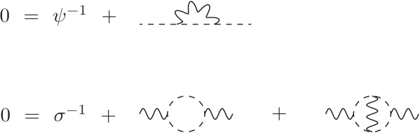
Figure 1: Leading order skeleton Schwinger-Dyson equations used to determine $\omega_{1}$ in the Gross-Neveu-Yukawa model.

3 Critical exponent $\omega_{1}$.

The method to find $\omega_{1}$ is to substitute the asymptotic scaling forms for the propagators and $2$-point functions into the skeleton Schwinger-Dyson equations. The relevant Feynman diagrams are given in Figure $1$ which merit several comments. First, the ordering of large $N$ graphs differs from that of ordinary coupling constant perturbation theory in that the corresponding parameter is $1/N$. However, as $N$ can emerge from the evaluation of a graph, when, for example, there is a closed fermion loop, then two and three loop graphs can actually be the same order in large $N$ perturbation theory. This is the case in scalar $O(N)$ theories but the same feature does not occur until $O(1/N^{2})$ in the Gross-Neveu universality class. This is because a loop with a trace over an odd number of $\gamma$-matrices vanishes. Also a reordering can occur for other reasons which we will discuss shortly. As the parameter $z$ also arises in the value of a graph and is $O(1/N)$ one counts a $\psi^{i}$ line as unity but a $\sigma$ field is $O(1/N)$. So in Figure $1$ the first graph of the $\sigma$ $2$-point is regarded as $O(N)$ but the subsequent graph is $O(1)$. There are no other graphs contributing to this $2$-point function at $O(1)$. In perturbation there would be additional graphs such as self-energy corrections to the leading order graph. These are not present in the large $N$ expansion since these contributions are contained in the anomalous parts of $\alpha$ and $\beta$. Including such self-energy corrected graphs would lead to overcounting, [12]. When substituting (2.9) and (2.14) into the graphs of Figure $1$ the subsequent algebraic equations for each $2$-point function decouple into two equations. This is because the corrections to scaling terms have a different power of $x^{2}$. So, for example, the set at leading order is

$$0~{}=~{}r(\alpha-1)~{}+~{}z~{}~{}~{},~{}~{}~{}0~{}=~{}p(\beta)~{}+~{}Nz$$ (3.1)

from which the earlier values for $\eta_{1}$ and $z_{1}$ follow.

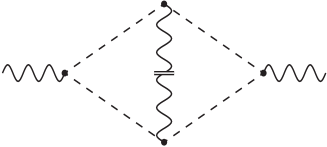
Figure 2: Diagram corresponding to $\Pi_{1B}$ where the double line indicates the inclusion of the correction to scaling exponent.

The remaining set require a more careful treatment, [17, 18, 20], due to a reordering alluded to earlier. This arises from considering the value of the function $q(\beta)$ when the canonical dimensions for the $\sigma$ field and $\omega$ are substituted. In particular the function $a(\beta-\mu+\omega)$ is $O(1/N)$. In the scalar $O(N)$ theory considered in the original large $N$ treatment of [12, 13] the corresponding function was $O(1)$ for the $\beta$-function of the two dimensional theory. With respect to the four dimensional $\beta$-function of that universality class there is a similar reordering to that of the Gross-Neveu universality class, [23]. The upshot is that the two loop graph of the $\sigma$ skeleton Schwinger-Dyson equation cannot be omitted and the two equations required for $\omega_{1}$ are

$$0 = r(\alpha-1)[1-A^{\prime}s(\alpha-1)(x^{2})^{\omega}]~{}+~{}z[1+(A^{\prime}+B^{\prime})(x^{2})^{\omega}]$$

$$0 = p(\beta)[1-B^{\prime}q(\beta)(x^{2})^{\omega}]~{}+~{}Nz[1+2A^{\prime}(x^{2})^{\omega}]$$ (3.2)

$$-~{}\frac{1}{2}Nz^{2}[\Pi_{1}+(\Pi_{1A}A^{\prime}+\Pi_{1B}B^{\prime})(x^{2})^{\omega}]$$

where we have split the contribution from the two loop $\sigma$ graph into its contributions relative to scaling corrections. This is because one contribution from the parts corresponding to the corrections to scaling are of the same order in $1/N$ as that from $q(\beta)$. The leading term, $\Pi_{1}$, is not needed for the equations determining $\eta_{1}$, (3.1), but are necessary for $\eta_{2}$ together with its counterpart in the $\psi^{i}$ $2$-point equation, [15]. The terms of (3.2) which involve $(x^{2})^{\omega}$ decouple from the corresponding terms of (3.1) to leave two equations involving the correction amplitudes $A^{\prime}$ and $B^{\prime}$. Representing these as a $2$ $\times$ $2$ matrix the consistency equation which determines $\omega_{1}$ is given by setting the determinant of this matrix to zero similar to the exponent for the critical $\beta$-function slope for the two dimensional Gross-Neveu model, [17, 18, 20].

Examining this consistency equation the only quantity which is required for finding $\omega_{1}$ is the value of the integral denoted by $\Pi_{1B}$. The notation is such that the letter $B$ means that the correction to scaling is included on the $\sigma$ line and the actual graph is illustrated in Figure $2$. From the consistency equation the large $N$ reordering that requires $\Pi_{1B}$ for $\omega_{1}$ is such that the other correction to scaling of this two loop graph, $\Pi_{1A}$, will first arise in the determination of $\omega_{2}$. In Figure $2$ the double line on the $\sigma$ line indicates that the exponent of that line is $\beta$ $-$ $\omega$ whereas the exponent on each fermion line is $\alpha$. Unlike conventional perturbation theory the exponents of these lines depend on the parameter $N$ and moreover the coefficient of that term in the exponent are the terms of the expansions such as (2.7). So the graph aside from being a function of $\mu$ due to the canonical dimensions of the fields is also a function of $N$. However, for $\omega_{1}$ only the leading term in $1/N$ is required. The $O(1/N)$ correction to $\Pi_{1B}$ will contribute to $\omega_{2}$.

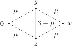
Figure 3: Feynman graph corresponding to $\Pi_{1B}$ with exponents included where $x$, $y$ and $z$ are the location of the vertices in coordinate space.

Substituting the canonical dimensions for the fields and $\omega$ produces the graph of Figure $3$. While the exponents of the lines are non-unit it is possible to evaluate the leading order term of the graph as a function of $\mu$ exactly. We have included the location of the internal and external vertices in Figure $3$ as we use coordinate space integration techniques developed in [12, 13]. In coordinate space the integration is over the location of the vertices. The first step of the evaluation is to apply a conformal transformation based on the left external vertex in the language of [13] to the graph which produces the graph of Figure $4$. The transformation produces an overall minus sign as indicated there and there is still a trace over the two remaining fermion lines. The resulting triangle with scalar propagators is what is termed a one step from uniqueness triangle since the sum of the exponents comprising that triangle sum to $(\mu-1)$. For a triangle to be unique the sum of exponents has to be $\mu$. The one step from uniqueness rule has been given in [24] and by applying it to this integral the resulting set of graphs each involve simple coordinate space chain integrals in the language of [12, 13]. This produces

$$\Pi_{1B}~{}=~{}-~{}\frac{2(\mu^{2}-4\mu+2)}{(\mu-1)^{2}(\mu-2)\Gamma^{2}(\mu)}~{}+~{}O\left(\frac{1}{N}\right)$$ (3.3)

at leading order.

With this value for the integral it is a straightforward exercise to evaluate the determinant of the $\omega_{1}$ consistency equation at leading order in $1/N$ to obtain one of our main results

$$\omega_{1}~{}=~{}-~{}\frac{2(2\mu-1)(\mu-2)}{(\mu-1)}\eta_{1}~{}.$$ (3.4)

From (3.4) the $\epsilon$ expansion near $d$ $=$ $4$ $-$ $2\epsilon$ dimensions produces

$$\omega_{1}~{}=~{}12\epsilon^{2}~{}-~{}14\epsilon^{3}~{}-~{}11\epsilon^{4}~{}+~{}\left[24\zeta_{3}-\frac{19}{2}\right]\epsilon^{5}~{}+~{}O(\epsilon^{6})~{}.$$ (3.5)

Also in various odd dimensions we have

$$\left.\frac{}{}\omega\right|_{d=3} = -~{}\frac{1}{2}~{}+~{}\frac{32}{3\pi^{2}N}~{}+~{}O\left(\frac{1}{N^{2}}\right)$$

$$\left.\frac{}{}\omega\right|_{d=5} = \frac{1}{2}~{}+~{}\frac{512}{15\pi^{2}N}~{}+~{}O\left(\frac{1}{N^{2}}\right)$$ (3.6)

with the $\epsilon$ expansion around $d$ $=$ $2$ $-$ $2\epsilon$ being non-singular.

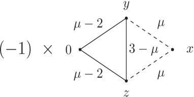
Figure 4: Feynman graph corresponding to $\Pi_{1B}$ after conformal left transformation.

The final stage of the exercise of computing $\omega_{1}$ is to check it against the explicit two and three loop $\overline{\mbox{MS}}$ perturbative $\beta$-functions, [10, 11]. We recall the expressions for the $\beta$-functions of [10] in the notation of that paper are

$$\beta_{1}(g_{1},g_{2}) = -~{}2\epsilon g_{1}~{}+~{}[2N+3]g_{1}^{2}$$

$$+~{}3[-16Ng_{1}^{2}-3g_{1}^{2}-64g_{1}g_{2}+64g_{2}^{2}]\frac{g_{1}}{8}$$

$$+~{}[224N^{2}g_{1}^{3}+864\zeta_{3}Ng_{1}^{3}+134Ng_{1}^{3}+912\zeta_{3}g_{1}^{3}-697g_{1}^{3}+5760Ng_{1}^{2}g_{2}$$

$$~{}~{}~{}+8064g_{1}^{2}g_{2}-5760Ng_{1}g_{2}^{2}+17472g_{1}g_{2}^{2}-13824g_{2}^{3}]\frac{g_{1}}{64}$$

$$+~{}[a_{1}g_{1}^{4}+a_{2}g_{1}^{3}g_{2}+a_{3}g_{1}^{2}g_{2}^{2}+a_{4}g_{1}g_{2}^{3}+a_{5}g_{2}^{4}]g_{1}N^{3}~{}+~{}O(g_{i}^{6})$$

$$\beta_{2}(g_{1},g_{2}) = -~{}2\epsilon g_{2}~{}+~{}[-Ng_{1}^{2}+4Ng_{1}g_{2}+36g_{2}^{2}]$$ (3.7)

$$+~{}[4Ng_{1}^{3}+7Ng_{1}^{2}g_{2}-72Ng_{1}g_{2}^{2}-816g_{2}^{3}]$$

$$+~{}[-628N^{2}g_{1}^{4}-384\zeta_{3}Ng_{1}^{4}+5Ng_{1}^{4}+3472N^{2}g_{1}^{3}g_{2}-3744\zeta_{3}Ng_{1}^{3}g_{2}$$

$$~{}~{}~{}-8790Ng_{1}^{3}g_{2}-3456N^{2}g_{1}^{2}g_{2}^{2}+31104\zeta_{3}Ng_{1}^{2}g_{2}^{2}+17328Ng_{1}^{2}g_{2}^{2}$$

$$~{}~{}~{}+49536Ng_{1}g_{2}^{3}+663552\zeta_{3}g_{2}^{4}+1002240g_{2}^{4}]\frac{1}{32}$$

$$+~{}[b_{1}g_{1}^{5}+b_{2}g_{1}^{4}g_{2}+b_{3}g_{1}^{3}g_{2}^{2}+b_{4}g_{1}^{2}g_{2}^{3}+b_{5}g_{1}g_{2}^{4}+b_{6}g_{2}^{5}]N^{3}~{}+~{}O(g_{i}^{6})$$

where $\zeta_{z}$ is the Riemann zeta function. We have included two sets of coefficients $a_{i}$ and $b_{i}$ which are the unknown coefficients in each of the four loop $\beta$-functions at leading order in large $N$. It may be the case that when they are known explicitly that some are actually zero. However knowledge of the $O(\epsilon^{4})$ term of $\omega_{1}$ will give a constraint on a linear combination of the unknown coefficients. To make the connection between the $\beta$-functions of (3.7) and $\omega_{1}$ is not as straightforward as connecting the $\beta$-function of the Gross-Neveu model with the analogous large $N$ critical exponent encoding it. This is because in that model there is only one coupling constant whereas in the Gross-Neveu-Yukawa case there are two coupling constants and hence two $\beta$-functions. So in the Gross-Neveu model evaluating the slope of the $\beta$-function at criticality it can be compared directly with the $\epsilon$ expansion of the corresponding critical exponent at each order in $1/N$, [15, 17, 18, 20]. For a two coupling theory like the Gross-Neveu-Yukawa model the quantity which is parallel to the $\beta$-function slope is the matrix of first order derivatives of $\beta_{i}(g_{1},g_{2})$ and defined by

$$\beta_{ij}(g_{1},g_{2})~{}=~{}\left(\frac{\partial\beta_{i}}{\partial g_{j}}\right)~{}.$$ (3.8)

To proceed we find the two eigenvalues of this matrix which are given by

$$\beta_{\pm}(g_{1},g_{2}) = \frac{1}{2}\left[\frac{}{}\beta_{11}(g_{1},g_{2})+\beta_{22}(g_{1},g_{2})\right.$$ (3.9)

$$\left.~{}~{}~{}\pm~{}\sqrt{\left[\left[\beta_{11}(g_{1},g_{2})-\beta_{22}(g_{1},g_{2})\right]^{2}+4\beta_{12}(g_{1},g_{2})\beta_{21}(g_{1},g_{2})\right]}\right]$$

from which we can obtain the two eigen-exponents at criticality defined by

$$\omega_{\pm}~{}=~{}\beta_{\pm}(g_{1c},g_{2c})$$ (3.10)

where the subscript _c indicates the value of the coupling constants at the Wilson-Fisher fixed point. The formal large $N$ expansion is given by

$$\omega_{\pm}~{}=~{}\sum_{n=0}^{\infty}\frac{\omega_{\pm\,n}}{N^{n}}$$ (3.11)

and from (3.7) we have

$$\omega_{-\,1}~{}=~{}-~{}6\epsilon^{2}~{}+~{}7\epsilon^{3}~{}+~{}3\left[a_{1}+\frac{a_{2}}{2}+\frac{a_{3}}{4}+\frac{a_{4}}{8}+\frac{a_{5}}{16}\right]\epsilon^{4}~{}+~{}O(\epsilon^{5})~{}.$$ (3.12)

Clearly this is in agreement with $\omega_{1}$ when allowance is made for the fact that the $\beta$-functions of (3.7) were derived for a spinor trace convention of $4$. Moreover the $O(\epsilon^{4})$ term gives the constraint

$$a_{1}~{}+~{}\frac{a_{2}}{2}~{}+~{}\frac{a_{3}}{4}~{}+~{}\frac{a_{4}}{8}~{}+~{}\frac{a_{5}}{16}~{}=~{}\frac{11}{6}$$ (3.13)

which corresponds to a blind test we alluded to earlier. A similar constraint can be constructed for the five loop $\beta$-function.

4 Non-abelian Nambu-Jona-Lasinio model.

Having determined $\omega_{1}$ for the ultraviolet completeness of the Gross-Neveu model it is possible to extend the formalism for related $4$-fermi models with continuous chiral symmetry. These come under the broad title of the Nambu-Jona-Lasinio model but there are several classes of such models depending on the group content. Moreover in the more recent language several are the ultraviolet completions of two dimensional models which have a different name associated with them. For instance the chiral Gross-Neveu (CGN) model is, [1, 25],

$$L_{\mbox{\footnotesize{CGN}}}~{}=~{}i\bar{\psi}^{i}\partial\!\!\!/\psi^{i}~{}+~{}g\left[\sigma\bar{\psi}^{i}\psi^{i}~{}+~{}i\pi\bar{\psi}^{i}\gamma^{5}\psi^{i}\right]~{}-~{}\frac{1}{2}[\sigma^{2}+\pi^{2}]$$ (4.1)

which is the extension of (2.1) from a theory with a discrete chiral symmetry to one with a continuous $U(1)$ chiral symmetry and involves an additional bosonic field. The Lagrangian is renormalizable in two dimensions and shares other properties with (2.1). We refer to it as the chiral Gross-Neveu model rather than the Nambu-Jona-Lasinio model as the latter is usually regarded as an effective theory describing meson states in four dimensions where it would be non-renormalizable. We will call the ultraviolet completion of (4.1) the chiral Gross-Neveu-Yukawa (CGNY) model which has the Lagrangian

$$L_{\mbox{\footnotesize{CGNY}}}~{}=~{}i\bar{\psi}^{i}\partial\!\!\!/\psi^{i}~{}+~{}\frac{1}{2}\partial_{\mu}\sigma\partial^{\mu}\sigma~{}+~{}\frac{1}{2}\partial_{\mu}\pi\partial^{\mu}\pi~{}+~{}g_{1}\left[\sigma\bar{\psi}^{i}\psi^{i}~{}+~{}i\pi\bar{\psi}^{i}\gamma^{5}\psi^{i}\right]~{}+~{}\frac{g_{2}^{2}}{24}\left(\sigma^{2}+\pi^{2}\right)^{2}$$ (4.2)

and has a $U(1)$ $\times$ $U(1)$ chiral symmetry. Like (2.2) $L_{\mbox{\footnotesize{CGNY}}}$ has an additional coupling constant compared to (4.1). In the context of extensions which relate more closely to the Standard Model the chiral Gross-Neveu model can be endowed with a non-abelian symmetry to produce the Lagrangian, [1],

$$L_{\mbox{\footnotesize{NJL}}}~{}=~{}i\bar{\psi}^{iI}\partial\!\!\!/\psi^{iI}~{}+~{}g\left[\sigma\bar{\psi}^{iI}\psi^{iI}~{}+~{}i\pi^{a}\bar{\psi}^{iI}\lambda^{a}_{IJ}\gamma^{5}\psi^{iJ}\right]~{}-~{}\frac{1}{2}\left[\sigma^{2}+{\pi^{a}}^{2}\right]$$ (4.3)

where $T^{a}$ $=$ $\mbox{\small{$\frac{1}{2}$}}\lambda^{a}$ are the Lie group generators. The additional indices have ranges $1$ $\leq$ $I$ $\leq$ $M$ and $1$ $\leq$ $a$ $\leq$ $N_{\!A}$ where $N_{\!A}$ is the dimension of the adjoint representation of the Lie group. We will call this the non-abelian Nambu-Jona-Lasinio model or universality class. This version was introduced in [1] where it was shown to be invariant under chiral $SU(M)$ $\times$ $SU(M)$ transformations. We use this form, (4.3), in order to be consistent with the notation of earlier large $N$ computations of critical exponents. The conventions of [26, 27] are retained and we recall that the Lie group Casimirs are

$$\mbox{Tr}(\lambda^{a}\lambda^{b})~{}=~{}4T_{F}\delta^{ab}~{}~{}~{},~{}~{}~{}\lambda^{a}\lambda^{a}~{}=~{}4C_{F}I~{}~{}~{},~{}~{}~{}f^{acd}f^{bcd}~{}=~{}C_{A}\delta^{ab}~{}.$$ (4.4)

Then the ultraviolet completeness of (4.3) is the non-abelian Nambu-Jona-Lasinio-Yukawa model

$$L_{\mbox{\footnotesize{NJLY}}} = i\bar{\psi}^{iI}\partial\!\!\!/\psi^{iI}~{}+~{}\frac{1}{2}\partial_{\mu}\sigma\partial^{\mu}\sigma~{}+~{}\frac{1}{2}\partial_{\mu}\pi^{a}\partial^{\mu}\pi^{a}$$ (4.5)

$$+~{}g_{1}\left[\sigma\bar{\psi}^{iI}\psi^{iI}~{}+~{}i\pi^{a}\bar{\psi}^{iI}\lambda^{a}_{IJ}\gamma^{5}\psi^{iJ}\right]~{}+~{}\frac{g_{2}^{2}}{24}\left(\sigma^{2}+{\pi^{a}}^{2}\right)^{2}~{}.$$

Given the similarity of the Lagrangians (4.1) and (4.3) we will focus on computing $\omega_{1}$ in the latter because the chiral Gross-Neveu Lagrangian follows by taking the abelian limit of the non-abelian Nambu-Jona-Lasinio model. By this we mean that formally $\lambda^{a}$ is replaced by the unit matrix and $\pi^{a}$ by the $\pi$ field in (4.3). For the resulting exponents this will correspond to the Casimirs taking the values $C_{F}$ $=$ $T_{F}$ $=$ $\frac{1}{4}$, $C_{A}$ $=$ $0$ and $M$ $=$ $1$.

As the large $N$ method for the non-abelian Nambu-Jona-Lasinio universal theory at the Wilson-Fisher fixed point is analogous to that used for the Gross-Neveu case we will indicate the major differences which have to be taken into account in order to deduce $\omega_{1}$. First, as there are three fields now the asymptotic scaling forms for the propagators and $2$-point functions are, [26, 27],

$$\psi(x) \sim \frac{Ax\!\!\!/}{(x^{2})^{\alpha}}\left[1+A^{\prime}(x^{2})^{\omega}\right]~{}~{}~{},~{}~{}~{}\sigma(x)~{}\sim~{}\frac{B}{(x^{2})^{\beta}}\left[1+B^{\prime}(x^{2})^{\omega}\right]$$

$$\pi(x) \sim \frac{C}{(x^{2})^{\gamma}}\left[1+C^{\prime}(x^{2})^{\omega}\right]$$ (4.6)

and

$$\psi^{-1}(x) \sim \frac{r(\alpha-1)x\!\!\!/}{A(x^{2})^{2\mu-\alpha+1}}\left[1-A^{\prime}s(\alpha-1)(x^{2})^{\omega}\right]$$ (4.7)

$$\sigma^{-1}(x) \sim \frac{p(\beta)}{B(x^{2})^{2\mu-\beta}}\left[1-B^{\prime}q(\beta)(x^{2})^{\omega}\right]$$

$$\pi^{-1}(x) \sim \frac{p(\gamma)}{C(x^{2})^{2\mu-\gamma}}\left[1-C^{\prime}q(\gamma)(x^{2})^{\omega}\right]$$ (4.8)

respectively in coordinate space where $C$ and $C^{\prime}$ are additional $x$-independent amplitudes. In this section our notation will primarily follow that of [26, 27]. The amplitude $C$ will appear within the skeleton Schwinger-Dyson equations in the combination $y$ $=$ $A^{2}C$ analogous to $z$. The dimensions of the respective fields are defined as

$$\alpha~{}=~{}\mu~{}+~{}\mbox{\small{$\frac{1}{2}$}}\eta~{}~{}~{},~{}~{}~{}\beta~{}=~{}1~{}-~{}\eta~{}-~{}\chi_{\sigma}~{}~{}~{},~{}~{}~{}\gamma~{}=~{}1~{}-~{}\eta~{}-~{}\chi_{\pi}$$ (4.9)

where $\chi_{\pi}$ is the anomalous dimension of the $3$-point vertex involving $\pi^{a}$. With the additional $\pi^{a}$ field the set of skeleton Schwinger-Dyson equation changes and these are illustrated in Figure $5$. The various two loop graphs in the $\sigma$ and $\pi^{a}$ $2$-point functions are again needed due to the same reordering as the Gross-Neveu model which is present here too.

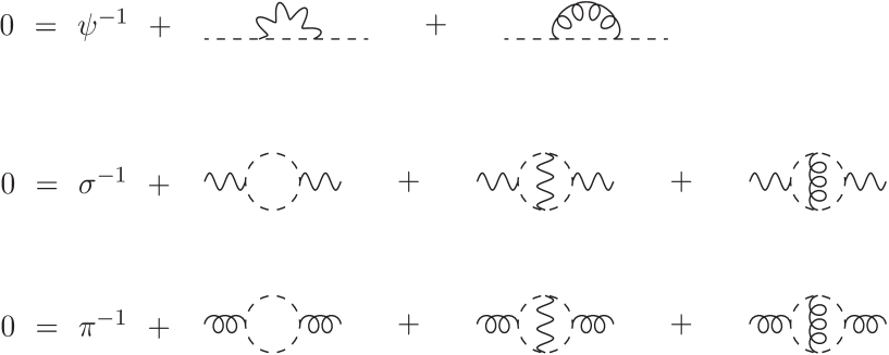
Figure 5: Leading order skeleton Schwinger-Dyson equations used to determine $\omega_{1}$ in the non-abelian Nambu-Jona-Lasinio model.

There are no mixed $\sigma$-$\pi^{a}$ $2$-point functions as would be allowed by the Feynman rules. This is because of the preservation of the chiral symmetry and general properties of $\gamma^{5}$. For instance, such mixing terms could be chirally rotated back to the set of Figure $5$. Moreover the role and presence of $\gamma^{5}$ in the $d$-dimensional context deserves comment. While there is no concept of chiral symmetry beyond even integer dimensions the matrix $\gamma^{5}$ is retained but is regarded as a formal object which obeys the naive anti-commutation relation

$$\{\gamma^{\mu},\gamma^{5}\}~{}=~{}0$$ (4.10)

in $d$-dimensions when an even number of $\gamma^{5}$’s are present. The other important aspect to stress is that while we are performing computations in $d$-dimensions the spacetime dimension has not been extended away from its critical dimension in order to effect a regularization of the theory in perturbation theory. In the large $N$ expansion method developed in [12, 13] divergent Feynman integrals are regularized analytically by shifting the vertex anomalous dimensions $\chi_{i}$ $\to$ $\chi_{i}$ $+$ $\Delta$ where $\Delta$ is the regularizing parameter. While the integrals we need here are finite in the large $N$ context, and hence do not need to be regularized, we mention the large $N$ regularization since it obviates the need to discuss how $\gamma^{5}$ is defined in this formalism. It is regarded as an object which obeys the above simple algebra in $d$-dimensions. This is consistent, for example, with the use of the $\epsilon$ expansion of critical exponents. Such expansions are invariably derived from theories in either two or four dimensions and then the $\epsilon$ expansion is summed before deducing an estimate in three dimensions. Strictly when one constructs such an $\epsilon$ expansion one has lost the chiral symmetry of the fixed even dimensional spacetime and then it is not the chiral symmetry as such which is the main property. Rather it is the preservation of the underlying anti-commutativity of $\gamma^{5}$ to bridge across the dimensions between two and four, and its properties to exclude a mixed $\sigma$-$\pi^{a}$ $2$-point function for example, which is the main guiding principal in $d$-dimensions. This anti-commutativity was also central to the associated large $N$ computations here.

Like the Gross-Neveu universality class we need the basic quantities for (4.3) in the large $N$ expansion. The leading order diagrams of Figure $5$ with the first terms of the scaling functions give, [26, 27],

$$0~{}=~{}r(\alpha-1)~{}+~{}z~{}+~{}4C_{F}y~{}~{}~{},~{}~{}~{}0~{}=~{}p(\beta)~{}+~{}2MNz~{}~{}~{},~{}~{}~{}0~{}=~{}p(\gamma)~{}+~{}8T_{F}Ny$$ (4.11)

from which it follows that, [26, 27],

$$\eta_{1}~{}=~{}\frac{\tilde{\eta}_{1}}{2}\left[\frac{1}{M}~{}+~{}\frac{C_{F}}{T_{F}}\right]~{}.$$ (4.12)

We have introduced the group independent exponent

$$\tilde{\eta}_{1}~{}=~{}-~{}\frac{2\Gamma(2\mu-1)}{\Gamma(\mu+1)\Gamma(\mu)\Gamma(1-\mu)\Gamma(\mu-1)}$$ (4.13)

which is core to both the chiral Gross-Neveu and non-abelian Nambu-Jona-Lasinio classes. Equally

$$z_{1}~{}=~{}\frac{\mu\Gamma^{2}(\mu)\tilde{\eta}_{1}}{4M}~{}~{}~{},~{}~{}~{}y_{1}~{}=~{}\frac{Mz_{1}}{4T_{F}}$$ (4.14)

and

$$\chi_{\sigma\,1}~{}=~{}\frac{\mu\tilde{\eta}_{1}}{2(\mu-1)}\left[\frac{1}{M}-\frac{C_{F}}{T_{F}}\right]~{}~{}~{},~{}~{}~{}\chi_{\pi\,1}~{}=~{}\frac{\mu\tilde{\eta}_{1}}{2(\mu-1)}\left[\frac{C_{F}}{T_{F}}-\frac{1}{M}-\frac{C_{A}}{2T_{F}}\right]$$ (4.15)

which are required to determine $\omega_{1}$. For orientation and for comparison to the Gross-Neveu skeleton Schwinger-Dyson equations at criticality we give the algebraic representation of the first two equations of Figure $5$ which are, [26, 27],

$$0 = r(\alpha-1)\left[1-A^{\prime}s(\alpha-1)(x^{2})^{\omega}\right]~{}+~{}z\left[1+(A^{\prime}+B^{\prime})(x^{2})^{\omega}\right]$$

$$+~{}4C_{F}y\left[1+(A^{\prime}+C^{\prime})(x^{2})^{\omega}\right]$$

$$0 = \frac{p(\beta)}{N}\left[1-B^{\prime}q(\beta)(x^{2})^{\omega}\right]~{}+~{}2zM\left[1+2A^{\prime}(x^{2})^{\omega}\right]~{}-~{}z^{2}M\left[\Pi+(A^{\prime}\Pi_{1A}+B^{\prime}\Pi_{1B})(x^{2})^{\omega}\right]$$ (4.16)

$$+~{}4yzMC_{F}\left[\Pi+(\Pi_{1A}A^{\prime}~{}+~{}\Pi_{1C}C^{\prime})(x^{2})^{\omega}\right]$$

where $\Pi_{1C}$ is the value of the analogous graph to that illustrated in Figure $2$. Although the leading order value in the $1/N$ expansion is the same as $\Pi_{1B}$ the corrections will be different since the value of the vertex anomalous dimension are different for the $3$-point vertices. With the extra field present the consistency equation to deduce $\omega_{1}$ is derived from ensuring that the determinant of the matrix formed by the three equations with respect to the vector $(A^{\prime},B^{\prime},C^{\prime})$ is zero. The three equations are

$$0 = \left[z+4C_{F}y-r(\alpha-1)s(\alpha-1)\right]A^{\prime}~{}+~{}zB^{\prime}~{}+~{}4C_{F}yC^{\prime}$$

$$0 = 4zA^{\prime}~{}-~{}\left[\frac{p(\beta)q(\beta)}{NM}+z^{2}\Pi_{1B}\right]B^{\prime}~{}+~{}4C_{F}yz\Pi_{1C}C^{\prime}$$

$$0 = 16T_{F}yA^{\prime}~{}+~{}4T_{F}yz\Lambda_{1B}B^{\prime}~{}-~{}\left[\frac{p(\gamma)q(\gamma)}{N}~{}+~{}8[2C_{F}-C_{A}]T_{F}y^{2}\Lambda_{1C}\right]C^{\prime}$$ (4.17)

where we designate the two loop correction graphs analagous to that of Figure $2$ but with $\pi^{a}$ external legs by the letter $\Lambda$, [27]. Again the leading order large $N$ values of $\Lambda_{1B}$ and $\Lambda_{1C}$ are the same as $\Pi_{1B}$. Solving the determinant at leading order produces

$$r(\alpha-1)s(\alpha-1)\left[2q(\beta)~{}-~{}z\left[1-\frac{C_{F}M}{T_{F}}\right]\Pi_{1B}\right]~{}=~{}4z\left[1+\frac{C_{F}M}{T_{F}}\right]$$ (4.18)

which contains $\omega_{1}$ as the only unknown where we have rewritten all the two loop graphs in terms of $\Pi_{1B}$, with value given in (3.3), which is valid at this order in the $1/N$ expansion. This would not be valid for finding $\omega_{2}$. Finally, this produces the result

$$\omega^{\mbox{\footnotesize{NJL}}}_{1}~{}=~{}-~{}\frac{(2\mu-1)(\mu-2)}{(\mu-1)}\left[\frac{1}{M}+(\mu-2)\frac{C_{F}}{T_{F}}\right]\tilde{\eta_{1}}~{}.$$ (4.19)

Taking the abelian limit gives the analogous quantity for (4.1) which is

$$\omega^{\mbox{\footnotesize{CGN}}}_{1}~{}=~{}-~{}(2\mu-1)(\mu-2)\tilde{\eta_{1}}~{}.$$ (4.20)

From these we find

$$\omega^{\mbox{\footnotesize{CGN}}}_{1} = 12\epsilon^{2}~{}-~{}26\epsilon^{3}~{}+~{}3\epsilon^{4}~{}+~{}O(\epsilon^{5})$$

$$\omega^{\mbox{\footnotesize{NJL}}}_{1} = \frac{12}{M}\epsilon^{2}~{}-~{}\left[12\frac{C_{F}}{T_{F}}+\frac{14}{M}\right]\epsilon^{3}~{}+~{}\left[14\frac{C_{F}}{T_{F}}-\frac{11}{M}\right]\epsilon^{4}~{}+~{}O(\epsilon^{5})$$ (4.21)

when $d$ $=$ $4$ $-$ $2\epsilon$. Equally

$$\left.\frac{}{}\omega^{\mbox{\footnotesize{CGN}}}\right|_{d=3} = -~{}\frac{1}{2}~{}+~{}\frac{16}{3\pi^{2}N}~{}+~{}O\left(\frac{1}{N^{2}}\right)$$

$$\left.\frac{}{}\omega^{\mbox{\footnotesize{CGN}}}\right|_{d=5} = \frac{1}{2}~{}+~{}\frac{256}{5\pi^{2}N}~{}+~{}O\left(\frac{1}{N^{2}}\right)$$ (4.22)

and

$$\left.\frac{}{}\omega^{\mbox{\footnotesize{NJL}}}\right|_{d=3} = -~{}\frac{1}{2}~{}-~{}\frac{16[C_{F}M-2T_{F}]}{3\pi^{2}T_{F}MN}~{}+~{}O\left(\frac{1}{N^{2}}\right)$$

$$\left.\frac{}{}\omega^{\mbox{\footnotesize{NJL}}}\right|_{d=5} = \frac{1}{2}~{}+~{}\frac{256[2T_{F}+C_{F}M]}{15\pi^{2}T_{F}MN}~{}+~{}O\left(\frac{1}{N^{2}}\right)$$ (4.23)

for various odd dimensions.

5 Discussion.

We have evaluated the critical exponent $\omega$ at $O(1/N)$ in the Gross-Neveu universality class as a function of $d$. It is the exponent which relates to the $\beta$-functions of the four dimensional Gross-Neveu-Yukawa theory which is not unrelated to the Standard Model. In addition we have found $\omega_{1}$ for two other cases which are the chiral Gross-Neveu and non-abelian Nambu-Jona-Lasinio universality classes. The actual large $N$ computation differed from the parallel one for the $\beta$-function exponent of the two dimensional Gross-Neveu model itself in that due to a reordering within the critical point large $N$ formalism a two loop graph had to be determined in order to deduce $\omega_{1}$. While it was a straightforward exercise to achieve this using conformal integration methods for massless integrals it means that the evaluation of $\omega_{2}$ will involve the computation of various three and four loop Feynman graphs contributing to the $\sigma$ skeleton Schwinger-Dyson equation. This would be the natural extension of the present work. Equally the comparison with four dimensional perturbation theory was not as straightforward compared to the two dimensional case. The Gross-Neveu-Yukawa model has two coupling constants and hence two $\beta$-functions which means that the comparison of the large $N$ exponent is with one of the eigenvalues of the Hessian of the $\beta$-functions at criticality. In terms of the underlying universal theory the two coupling constants can be viewed in a different way. Clearly the Gross-Neveu-Yukawa theory is renormalizable in four dimensions. However, away from four dimensions the operators associated with each coupling constant are different in $d$-dimensions and hence the degeneracy is lifted. At the Wilson-Fisher fixed point, which the large $N$ formalism used here operates at, the core interaction which drives the Gross-Neveu universality class is the $\sigma\bar{\psi}\psi$ one. The quartic $\sigma$ interaction in some sense spectates in four dimensions but is either relevant or irrelevant away from this dimension. Another way of putting this is that the canonical dimensions of each operator are the same in four dimensions but away from four dimensions they are no longer equal and therefore there is no degeneracy of the couplings. In other words in the dimension where the operators overlap there is a mixing which manifests itself as two $\beta$-functions in perturbation theory but operator mixing in the large $N$ universal theory. This is the reason why we had the more involved comparison with perturbation theory in contrast to [15, 17, 18, 20]. Viewing this aspect of the Gross-Neveu-Yukawa theory it is not inconsistent with the emergent supersymmetry which has been noticed recently, [7]. It is well known that supersymmetry is a symmetry of an integer dimension. Away from say four dimensions the degrees of freedom of the bosons and fermions are no longer equivalent. Indeed to consistently dimensionally regularize a supersymmetric theory is not possible because of this. One method to ameliorate this loss of equality was devised in [28] and requires extra fields which live only in the dimensionally extended part of the spacetime. At the emergent supersymmetric fixed point one would have to preserve the equivalence along the Wilson-Fisher fixed point in $d$-dimensions of its corresponding universal theory.

Acknowledgements. The author thanks R.M. Simms, Dr L. Mihaila and Dr M. Scherer for valuable discussions. The work was carried out with the support of the STFC through the Consolidated Grant ST/L000431/1. The graphs were drawn with the Axodraw package [29].

- [1] D. Gross & A. Neveu, Phys. Rev. D10 (1974), 3235.
- [2] J. Ashkin & E. Teller, Phys. Rev. 64 (1943), 178.
- [3] A.B. Zamolodchikov & A.B. Zamolodchikov, Ann. Phys. 120 (1979), 253.
- [4] P. Forgacs, F. Niedermayer & P. Weisz, Nucl. Phys. B367 (1991), 123.
- [5] L. Janssen & I.F. Herbut, Phys. Rev. B89 (2014), 205403.
- [6] K. Diab, L. Fei, S. Giombi. I.R. Klebanov & G. Tarnopolsky, J. Phys. A49 (2016), 405402.
- [7] L. Fei, S. Giombi, I.R. Klebanov & G. Tarnopolsky, Prog. Theor. Exp. Phys. (2016), 12C105.
- [8] S. Giombi, Higher Spin-—CFT Duality in Proceedings Theoretical Advanced Study Institute in Elementary Particle Physics: New Frontiers in Fields and Strings (TASI 2015), Boulder, USA, (2017), 137.
- [9] J. Zinn-Justin, Nucl. Phys. B367 (1991), 105.
- [10] L.N. Mihaila, N. Zerf, B. Ihring, I.F. Herbut & M.M. Scherer, arXiv:1703.08801 [cond-mat.str-el].
- [11] B. Rosenstein, H.-L. Yu & A. Kovner, Phys. Lett. B314 (1993), 381.
- [12] A.N. Vasil’ev, Y.M. Pismak & J.R. Honkonen, Theor. Math. Phys. 46 (1981), 104.
- [13] A.N. Vasil’ev, Y.M. Pismak & J.R. Honkonen, Theor. Math. Phys. 47 (1981), 465.
- [14] A.N. Vasil’ev, Y.M. Pismak & J.R. Honkonen, Theor. Math. Phys. 50 (1982), 127.
- [15] J.A. Gracey, Int. J. Mod. Phys. A6 (1991), 395, 2755(E).
- [16] J.A. Gracey, Phys. Lett. B297 (1992), 293.
- [17] S.É. Derkachov, N.A. Kivel, A.S. Stepanenko & A.N. Vasil’ev, hep-th/9302034.
- [18] A.N. Vasil’ev, S.É. Derkachov, N.A. Kivel & A.S. Stepanenko, Theor. Math. Phys. 94 (1993), 179.
- [19] A.N. Vasil’ev, & A.S. Stepanenko, Theor. Math. Phys. 97 (1993), 364.
- [20] J.A. Gracey, Int. J. Mod. Phys. A9 (1994), 567.
- [21] J.A. Gracey, Int. J. Mod. Phys. A9 (1994), 727.
- [22] A. Hasenfratz & P. Hasenfratz, Phys. Lett. B297 (1992), 166.
- [23] D.J. Broadhurst, J.A. Gracey & D. Kreimer, Z. Phys. C75 (1997), 559.
- [24] A.N. Vasil’ev, The Field Theoretic Renormalization Group in Critical Behavior Theory and Stochastic Dynamics (Chapman & Hall/CRC, Boca Raton, Florida, USA, 2004).
- [25] Y. Nambu & G. Jona-Lasinio, Phys. Rev. 122 (1961), 345.
- [26] J.A. Gracey, Phys. Lett. B308 (1993), 65.
- [27] J.A. Gracey, Z. Phys. C61 (1994), 115.
- [28] W. Siegel, Phys. Lett. B94 (1980), 37.
- [29] J.C. Collins & J.A.M. Vermaseren, arXiv:1606.01177 [cs.OH].