Online codes for analog signals

Abstract.

This paper revisits a classical scenario in communication theory: a waveform sampled at regular intervals is to be encoded so as to minimize distortion in its reconstruction, despite noise. This transformation must be online (causal), to enable real-time signaling; and should use no more power than the original signal. The noise model we consider is an “atomic norm” convex relaxation of the standard (discrete alphabet) Hamming-weight-bounded model: namely, adversarial $\ell_{1}$-bounded. In the “block coding” (noncausal) setting, such encoding is possible due to the existence of large almost-Euclidean sections in $\ell_{1}$ spaces, a notion first studied in the work of Dvoretzky in 1961. Our main result is that an analogous result is achievable even causally. Equivalently, our work may be seen as a “lower triangular” version of $\ell_{1}$ Dvoretzky theorems. In terms of communication, the guarantees are expressed in terms of certain time-weighted norms: the time-weighted $\ell_{2}$ norm imposed on the decoder forces increasingly accurate reconstruction of the distant past signal, while the time-weighted $\ell_{1}$ norm on the noise ensures vanishing interference from distant past noise. Encoding is linear (hence easy to implement in analog hardware). Decoding is performed by an LP analogous to those used in compressed sensing.

Keywords: Online coding, Dvoretzky theorems, Analog signals, Random matrices.

1. Introduction

1.1. The problem

We study a fundamental scenario of communication theory. A source is generating a waveform which we sample at regular intervals. We wish to encode the signal in real time, and decode the noise-affected transmission in real time, all while minimizing distortion in the reconstruction.

We require that the power (the $\left\|\cdot\right\|_{2}$ norm) of the transmission $\mathcal{E}(x)$ not exceed a constant factor of the power of the signal $x$; for simplicity of operation, we also wish the encoding map $\mathcal{E}$ to be linear and deterministic. We operate in a worst-case model, namely, the adversary has advance knowledge of the signal and its encoding. Furthermore, at a minimum, we wish to have the following kind of decoding guarantee: for any signal $x:\mathbb{N}\to\mathbb{R}$, and any bounded-power adversary noise $y:\mathbb{N}\to\mathbb{R}$ (i.e., $\left\|y\right\|_{2}<\infty$), the “limiting decoding” $\mathcal{D}(\mathcal{E}(x)+y)$ should equal $x$.

Actually, much of our effort will be devoted to stronger results quantifying the rate with which the decoder can eliminate noise. For this we must examine more closely the strength of the adversary. A conventional approach in analog communications would be to allow noise $y$ such that $\left\|y\right\|_{2}$ is small compared with $\left\|x\right\|_{2}$. This is indeed the standard framework in analog communication in which one first source-codes the signal using vector quantization, then channel-codes the now discrete signal using a finite alphabet, which, in turn, is encoded with a waveform. We would like, however to allow noise of comparable power to the signal, $\|y\|_{2}\leq O(\|x\|_{2})$, and even beyond.

It is immediately apparent, however, is that this kind of $\left\|\cdot\right\|_{2}$-bounded adversary is too powerful for the problem we consider: the adversary can assign $y=-\mathcal{E}(x)$ and simply zero-out the transmission.

However, a power constraint is only one plausible assumption on the noise source. The goal of our work is to show that if instead of the power constraint on the adversary, we make a different but very familiar assumption, we can provide an entirely different approach to this communication problem.

In our setting, where the noise is generated by an adversary, an alternative modeling assumption for noise is one that has proven fruitful as a model for signals in the compressed sensing literature: it is that the signal is bounded in (a possibly weighted) $\left\|\cdot\right\|_{1}$ norm. An $\left\|\cdot\right\|_{1}$ norm bound (for a signal of given power) is a kind of sparsity assumption, and sparsity is a natural characteristic of many signal sources, which is in large part why this approach has succeeded in compressed sensing [Don06]. It is therefore natural to pose the problem of protecting our signal against interference by sparse signals generated by an adversary. Indeed, in the context of digital error-correcting codes, the most basic and prevalent model has long been of noise limited in Hamming norm, which is precisely a sparsity assumption. Relaxations of such combinatorial sparsity assumptions to convex norms such as $\left\|\cdot\right\|_{1}$ are also used to make them amenable to convex programming formulations [CRPW12].

Methodologically, the approach of considering adversaries bounded in the same norm as the signal has a fundamental limitation: no deterministic coding method can recover the signal to accuracy better than the signal-to-noise ratio. On the other hand, focusing on an adversary bounded in a different norm than the signal (here $\left\|\cdot\right\|_{1}$ rather than $\left\|\cdot\right\|_{2}$) opens the possibility of achieving in the limit noise-free decoding. That, as well as convergence rates to this limit, is the contribution of this paper: power-limited, real-time communications against an $\left\|\cdot\right\|_{1}$-bounded adversary.

1.2. An easier problem: block coding

Undoubtedly, as for any error-correction problem, the most basic problem which one must consider here is that of block coding a signal. That is, the incoming signal is a vector $x\in\mathbb{R}^{T}$. We transmit at rate $1/\rho$, that is, we map $x$ to $\mathcal{E}(x)\in\mathbb{R}^{\rho T}$. Our first constraint on the encoder is an energy constraint. If the encoder could amplify the signal by an arbitrarily large factor, then it could swamp out any interference by an adversary who is bounded in power or any other norm. Since this is an unrealistic (and uninteresting) model for the encoder, we stipulate that the total power of the transmission should be comparable to the total power of the original message itself. That is, we ask that

$$\left\|\mathcal{E}(x)_{[\rho t]}\right\|_{2}\leq\left\|x_{[t]}\right\|_{2},\text{ for all $t\in[T]$}.$$ (*)

(Here $*_{[t]}$ denotes the prefix of a vector consisting of its first $t$ co-ordinates.) The noise source adds a vector $y\in\mathbb{R}^{T\rho}$ onto $\mathcal{E}(x)$; the noise $y$ may depend upon $\mathcal{E}(x)$. The receiver then applies a decoding map $\mathcal{D}\left(\mathcal{E}\left(x\right)+y\right)$. The question is then what can be achieved in terms of simultaneously

• Maximizing communication rate (minimizing $\rho$),

• Minimizing distortion relative to noise, i.e., minimizing the ratio $\frac{\left\|\mathcal{D}(\mathcal{E}(x)+y)-x\right\|_{2}}{\left\|y\right\|_{1}}$

As we discuss in more detail below, the answer to this question, although not posed in this language, was given long ago in the work of Milman [Mil71], Kašin [Kaš77], and Figiel, Lindenstrauss and Milman [FLM77], pursuing the study initiated by Dvoretzky [Dvo61] of Euclidean sections in Banach spaces. Further, the codes so achieved are linear: the encoding operation consists of multiplying the source vector by an appropriate $\rho T\times T$ matrix $A$, and the distortion ratio achieved is $O(T^{-1/2})$ (see discussion leading to eq. 8 below):

$$\left\|\mathcal{D}(\mathcal{E}(x)+y)-x\right\|_{2}\leq O(T^{-1/2})\left\|y\right\|_{1}.$$ (1)

In contrast, our object of study in this paper is the real-time or causal encoding and decoding of a source generated on the fly, as for instance an audio signal, or the signal from a remote sensor, in a distributed control setting. While the guarantees achieved in the offline (block coding) setting do serve as a guideline for framing what might be achievable in online coding, it will be clear from later discussions that not everything achievable offline can be achieved in the online setting.

We now proceed to formulate the appropriate requirements for the online setting. The encoder $\mathcal{E}$ is required to be such that the transmissions $1,\ldots,\rho t$ can depend only on the prefix $x_{[t]}$ of the message that is available to the source at time $t$: in other words, $\rho\geq 1$ symbols are sent for each symbol of the message, in a way such that these $\rho$ symbols depend only on the prefix $x_{[t]}$ of the message available at time $t$. In particular this enforces that

$$\mathcal{E}(x)_{[\rho t]}=\mathcal{E}(x_{[t]}),\text{ for all $t\in[T]$}.$$ (**)

The decoder is now a collection of maps from $\mathbb{R}^{\rho t}$ to $\mathbb{R}^{t}$ for each $t\in[T]$; the output of the decoder at time $t$ is $\mathcal{D}\left(\mathcal{E}\left(x_{[t]}\right)+y\right)$, where $y\in\mathbb{R}^{\rho t}$ is the unknown error introduced by the adversary up to time $t$.

As in the offline setting, we would like our encoder to be linear. The requirement in eq. ** then implies that the matrix $A$ implementing the encoder needs to be lower triangular in the rate-adjusted sense that $A_{i,j}=0$ if $i<j\rho$. (This is what we shall mean by “lower triangular” from here on.) However, none of the constructions arising from the work on Euclidean sections cited above provide a lower triangular $A$. This is to be expected since our decoding requirement in eq. 1 is itself unreasonable in the online setting: for example, an adversary who is silent for a while and then inserts a brief burst of noise can satisfy the $\left\|\cdot\right\|_{1}$ bound over the history of the communication, yet obliterate the last $\rho$ transmissions, which are the only ones to carry information about the most recent portion of the signal.

The above objection guides us toward the right decoding requirement in the online setting. The idea is that the inaccuracy in the decoding of a prefix $(x_{1},\ldots x_{t}),$ of the signal should decrease as time elapses after $t$, provided that the noise (even if adversarial) is subject to a possibly time-weighted $\left\|\cdot\right\|_{1}$-norm bound. Our aim is that for that portion of the signal that is in the remote past, our decoding guarantee is analogous to what can be achieved in the block coding setting. We now develop this idea quantitatively.

1.3. Two inadequate definitions

We start with two extreme formalizations, each of which captures one desirable feature; and then combine these. The first desideratum is that for any fixed $i$, as time $t$ goes on, our decoding of $x_{i}$ at time $t$ become ever-more accurate provided that the noise is below tolerable limits. (And in particular if the adversary stops injecting noise into the system.) This is analogous to the decoding guarantee given for discrete alphabets by tree codes.

We can formulate such a guarantee using a time-weighted norm for the decoding error. For a vector $x\in\mathbb{R}^{T}$, we define the $\left\|\cdot\right\|_{\star}$ “decoding norm”, in which the error on inputs from the remote past is given higher weight than that on recent inputs:

$$\left\|x\right\|_{\star}\mathrel{\hbox to0.0pt{\raisebox{1.29167pt}{$\cdot$}\hss}\raisebox{-1.29167pt}{$\cdot$}}=\left\|x\right\|_{\star(T)}\mathrel{\hbox to0.0pt{\raisebox{1.29167pt}{$\cdot$}\hss}\raisebox{-1.29167pt}{$\cdot$}}=\sqrt{\frac{1}{T}\sum_{i=1}^{T}(T-i+1)x_{i}^{2}},$$ (2)

and we modify the block-code decoding requirement (eq. 1) to the following:

$$\left\|\mathcal{D}(\mathcal{E}(x_{[t]})+y)-x_{[t]}\right\|_{\star(t)}\leq\frac{\left\|y\right\|_{1}}{t^{1/2-\delta}},\quad\text{for all $t\in[T]$ and any given fixed $\delta\in(0,1/2)$}.$$ (3)

The flaw in this definition is that once the adversary has ever injected noise into the system, no decoding is ever possible of signals in the recent past (i.e., of $x_{t-c}$ at time $t$ for small $c$), even if say the adversary has ceased to inject any noise after a fixed time $t_{0}$. That is, requirement (3) fails a second desideratum: that the effects of any noise burst should dissipate over time.

This leads us to the other extreme: a decoding guarantee in which noise from the distant past is allowed to contribute only vanishingly to the decoding error. For this we define the time-weighted “noise norm” $\left\|\cdot\right\|_{\dagger}$:

$$\left\|y\right\|_{\dagger}\mathrel{\hbox to0.0pt{\raisebox{1.29167pt}{$\cdot$}\hss}\raisebox{-1.29167pt}{$\cdot$}}=\left\|y\right\|_{\dagger(\rho T)}\mathrel{\hbox to0.0pt{\raisebox{1.29167pt}{$\cdot$}\hss}\raisebox{-1.29167pt}{$\cdot$}}=\sum_{i=1}^{\rho T}\left|y_{i}\right|\left(\frac{\rho T-i+1}{\rho T}\right)^{-1/2},$$ (4)

and impose again the decoding requirement

$$\left\|\mathcal{D}(\mathcal{E}(x_{[t]})+y)-x_{[t]}\right\|_{2}\leq\frac{\left\|y\right\|_{\dagger(t)}}{t^{1/2-\delta}},\quad\text{for all $t\in[T]$ and any given fixed $\delta\in(0,1/2)$}.$$ (5)

The flaw in this second definition is that it does not provide gradually-improving decoding of each fixed input character (which was the motivation for the first definition). For any fixed level of noise, we have no better decoding guarantee on $x_{1}$ than on $x_{T}$ at time $T$. (In particular, a bounded noise burst at time $T$ is enough to ruin the decoding of $x_{1}$.)

1.4. The satisfactory definition and our main result

We achieve both desiderata with a definition which time-weights both the adversary’s noise and the decoding error. Formally, for any $\mu\in[0,1]$, define

$$\left\|x\right\|_{\star_{\mu}} \mathrel{\hbox to0.0pt{\raisebox{1.29167pt}{$\cdot$}\hss}\raisebox{-1.29167pt}{$\cdot$}}=\left\|x\right\|_{\star_{\mu}(T)}\mathrel{\hbox to0.0pt{\raisebox{1.29167pt}{$\cdot$}\hss}\raisebox{-1.29167pt}{$\cdot$}}=\sqrt{\sum_{i=1}^{T}\left(\frac{T-i+1}{T}\right)^{\mu}x_{i}^{2}}$$ (6)

$$\left\|y\right\|_{\dagger_{\mu}} \mathrel{\hbox to0.0pt{\raisebox{1.29167pt}{$\cdot$}\hss}\raisebox{-1.29167pt}{$\cdot$}}=\left\|y\right\|_{\dagger_{\mu}(\rho T)}\mathrel{\hbox to0.0pt{\raisebox{1.29167pt}{$\cdot$}\hss}\raisebox{-1.29167pt}{$\cdot$}}=\sum_{i=1}^{\rho T}\left(\frac{\rho T-i+1}{\rho T}\right)^{-(1-\mu)/2}\left|y_{i}\right|.$$

This subsumes the earlier cases we considered: eq. 2 is the case $\mu=1$ while eq. 4 is the case $\mu=0$.

Now, given any choice of $\mu\in(0,1]$ and $\delta\in(0,1/2)$, we demand the decoding guarantee (generalizing eqs. 3 and 5):

$$\left\|\mathcal{D}(\mathcal{E}(x_{[t]})+y)-x_{[t]}\right\|_{\star_{\mu}(t)}\leq\frac{\left\|y\right\|_{\dagger_{\mu}(\rho t)}}{t^{1/2-\delta}},\quad\text{for all $t\in[T]$}.$$ (***)

Note that for any $\mu$, the penalty imposed by the $\left\|\cdot\right\|_{\star_{\mu}}$-norm for errors made in decoding entries far away in the past (say at times $s<ct$) is the same (to within a constant factor $c^{\prime}=c^{\prime}(c)$) as that imposed by the $\left\|\cdot\right\|_{2}$-norm. Similarly, the weight assigned by the $\left\|\cdot\right\|_{\dagger}$ norm to the adversary’s noise inserted at times $s<ct$ is within a constant factor to its unweighted $\left\|\cdot\right\|_{1}$ norm. However, when we are decoding entries $x_{s}$ for $s$ close to $t$, for which we do not yet have much information, these weighted norms allow us to make larger errors in decoding without much penalty. For $0<\mu\leq 1$, the requirement (*** ‣ 1.4) on the decoder guarantees that as time progresses, so does our ability to attenuate the error introduced by the adversary. Further, in Theorem 2.2, we show that our requirements enforce that the scaling of the attenuation factor in (*** ‣ 1.4) cannot be $O(t^{-1/2})$ and must be of the form $\omega(t^{-1/2})$. In this the online coding problem differs from the block coding or $\left\|\cdot\right\|_{1}$-Dvoretzky problem.

Our main result is that for any fixed $\mu\in(0,1]$ and any $\delta\in\left(0,\frac{1}{2}\right)$, there is a constant-rate, constant-power code achieving requirement (*** ‣ 1.4). Our code is linear, and decoding too is efficient: the decoder solves a linear program analogous to those appearing in the compressed sensing literature.

Notation. For a $\rho T\times T$ matrix $A$, we denote by $A_{t}$ the $\rho t\times t$ matrix consisting of its top $\rho t$ rows and leftmost $t$ columns.

Theorem 1.1 (Informal, see Theorem 2.1 for a formal statement).

For any $\mu\in(0,1]$ and $\delta\in(0,\frac{1}{2})$, there exists a rate parameter $\rho>0$ for which there exists an encoder $\mathcal{E}$ and a decoder $\mathcal{D}$ satisfying the energy, error attenuation, and causal constraints in eqs. (* ‣ 1.2), (** ‣ 1.2), and (*** ‣ 1.4).

In particular, the encoder $\mathcal{E}$ acts as left multiplication by a $\rho T\times T$ matrix $\mathcal{C}$ that is rate-adjusted lower triangular (i.e., $\mathcal{C}_{ij}=0$ when $i\leq(j-1)\rho$), where $T$ is the total time of transmission. At time $t\leq T$, the decoder $\mathcal{D}$ acts by making an $\left\|\cdot\right\|_{\dagger}$-norm projection to $\textup{{Range}}(\mathcal{C}_{t})$ and then applying $\mathcal{C}_{t}^{-1}$ (which is well defined on $\textup{{Range}}(\mathcal{C})$).

A natural special case of the above is with $\mu=1/2$. In this case the decoder and encoder guarantee

$$\sqrt{\sum_{i=1}^{T}\left(\frac{T-i+1}{T}\right)^{1/2}|\mathcal{D}(\mathcal{E}(x_{[t]})+y)_{i}-x_{i}|^{2}}\leq O(T^{\delta-1/2})\sum_{i=1}^{\rho T}\left(\frac{\rho T-i+1}{\rho T}\right)^{-1/4}|{y_{i}}|$$

In particular, if both the waveform values $x_{i}$ and the noise values $y_{i}$ are $\Theta(1)$, then the error incurred by the decoder on a given entry of the signal, decreases to zero (at almost a $T^{-1/2}$ pace) as the communication continues in time. We also note that the quantity $(1-\mu)$ appearing in the exponent of the gain factor used in the $\left\|\cdot\right\|_{\dagger_{\mu}}$ norm cannot be replaced by any strictly smaller quantity; see the remark following Theorem 2.1 for details.

1.5. Block coding and the Dvoretzky theorem

We now revisit the relation between Euclidean sections and block coding briefly alluded to above. Our goal in this paper may also be framed as showing the existence of a “lower triangular” analogue of a Euclidean section. This lower triangular constraint is the main source of technical difficulty in our work as compared to previous work; in particular, our method is quite different. The prior work does, however, show some limits on what can be achieved: specifically, it is enough to imply that the parameter $\delta$ in Theorem 1.1 has to be non-negative. In recent years, the classic work on Euclidean sections has been re-interpreted explicitly in coding-theoretic language in a line of work that seeks to derandomize the original constructions [AAM06, LS08, GLW08, GLR10, IS10]. We now sketch these connections.

Dvoretzky [Dvo61] initiated the study of the existence of large subspaces $S$ of $\mathbb{R}^{n}$ equipped with an arbitrary norm which are “close” to being Euclidean. Our interest here is in the case where the norm is an $\left\|\cdot\right\|_{p}$-norm with $p=1$, in which case the condition of $S$ being close to Euclidean can be written as

$$\sup_{x\in S}\frac{\sqrt{n}\left\|x\right\|_{2}}{\left\|x\right\|_{1}}\leq\Delta.$$

Here $\Delta$ is the distortion of the section, and one seeks to make it as close to $1$ as possible. The problem of finding Euclidean sections of large dimension has also been extensively studied, starting with the work of Figiel, Lindenstrauss and Milman, and of Kašin [Mil71, Kaš77, FLM77], and in the special case $p=1$ it is known that there exists a constant $c>1$ (depending on $\Delta$) such that $(\mathbb{R}^{cn},\left\|\cdot\right\|_{1})$ contains an Euclidean section of dimension $n$.

An equivalent view of Euclidean sections can be obtained in terms of a modified “condition number” of appropriate tall matrices (see, e.g., [FLM77]). In particular, if there exists a real $cn\times n$ matrix $A$ of rank $n$ such that

$$\left\|A\right\|_{2\rightarrow 2}\cdot\left\|A^{-1}\right\|_{1\rightarrow 2}\leq\frac{\Delta}{\sqrt{n}}$$ (7)

then $(\mathbb{R}^{cn},\left\|\cdot\right\|_{p})$ has a Euclidean section of dimension $n$ (namely, $\textup{{Range}}(A)$) with distortion at most $\Delta$ (Here, and subsequently, $A^{-1}$ denotes Moore-Penrose pseudo-inverse). It is also not hard to see that the existence of such a Euclidean section implies the existence of a rank $n$ $cn\times n$ matrix $A$ satisfying eq. 7.

This representation of an Euclidean section allows us to view it as a “block” version of the codes we seek in this paper. For, let $A$ be a matrix satisfying the constraint in eq. 7, and assume without loss of generality that $\left\|A\right\|_{2\rightarrow 2}=1$ (this can be ensured since the requirement in eq. 7 is invariant under scaling $A$ by constants). Define the encoder $\mathcal{E}$ as left multiplication by $A$: $\mathcal{E}(x)=Ax$. The decoder $\mathcal{D}$ acts on an input $y$ by first finding the point $y^{\prime}$ in $\textup{{Range}}(A)$ that is closest to $y$ in the $\left\|\cdot\right\|_{1}$-norm (choosing one arbitrarily if there are several such points), and then returning $A^{-1}y^{\prime}$. Since $\left\|A\right\|_{2\rightarrow 2}=1$, the energy constraint (eq. *) is satisfied automatically. Using eq. 7 it can also be shown that

$$\left\|\mathcal{D}(\mathcal{E}(x)+y)-x\right\|_{2}\leq\frac{2\Delta}{\sqrt{n}}\left\|y\right\|_{1}.$$ (8)

It is this guarantee for block decoding that we compare our result in Theorem 1.1 against.

1.6. Related work

We are following here on two main lines of work in communications. One is the investigation begun by Sahai and Mitter of the “anytime capacity” of a communication channel, which they discovered to be essential to the feasibility of using that channel to control an unstable plant in real time [SM06]. Several types of channels and noise have been studied but the primary concern in that literature is the role of channel noise in a feedback loop, and to our knowledge there is no result which resembles ours. The second concerns real-time communication of discrete signals over discrete channels; one of the results from that literature is that it is possible to causally encode a signal in such a manner that at all times $T$, if the noise has so far corrupted only $cT$ characters ($c>0$ sufficiently small), then the decoder can correctly determine the initial $(1-O(c))T$ characters [Sch96]. Our main result in this paper is intended as the appropriate analog of the latter statement for a physical signal and a physical channel, where “characters” are amplitudes of a waveform.

Our proof of existence of the code proceeds through an analysis of certain random matrices with independent but not identically distributed Gaussian entries. In this light, our requirements, especially when rephrased in terms similar to eq. 7, are connected to the long line of work on the condition number of almost square (and even square) random matrices (see, e.g, [ES05, Rud08, RV09, TV09] and the references therein). Note, however, that we are concerned here with an analogue of a $\left\|\cdot\right\|_{1\rightarrow 2}$-norm of the pseudo-inverse of the encoding matrix, while in the work on condition number the emphasis is on the $\left\|\cdot\right\|_{2\rightarrow 2}$ norm of the inverse. Further, much of the work on the condition number has considered rectangular random matrices with identically distributed entries (see, however, the work of Cook [Coo18] and Rudelson and Zeitouni [RZ16] for recent progress on the lowest singular value of a class of structured matrices with non-i.i.d. entries) while we are in a very different regime—the main technical challenge of our work is to deal with the pseudo-inverse of random lower triangular matrices (whose non-zero entries are also not identically distributed). Nevertheless, we believe that the techniques developed in the work on the condition number may be relevant for further improvements of our result, especially on the question of achieving an optimal rate. We also note in passing that if one is concerned only with the norm of a matrix with independent but not necessarily i.i.d. entries (rather than the norm of its pseudo-inverse) then there are results in the literature providing good asymptotic bounds (see, e.g., [Lat05, SR13, BvH16, LvHY18]). Our analysis in fact uses one of these bounds from the work of Bandeira and van Handel [BvH16].

A rather different notion of online coding underlies the long and celebrated line of work on fountain codes [BLMR98]. Recall that in our online coding setting, (1) the encoder does not receive the message symbols as a block but in an online fashion; (2) the adversary corrupts transmitted symbols rather than erasing them, so that the receiver does not know if a received symbol is corrupted or not; (3) both the original message and the transmission have real numbers as symbols. In fountain codes and continuing work such as LT codes [Lub02] and Raptor codes [Sho06] (see also [May02]), the setting is different: (1) even at time $t=0$, the encoder has access to the full block of $n$ symbols comprising the message; (2) the message is to be sent over an erasure channel; (3) both the source and transmission symbols come from a discrete alphabet. The goal is for the code to be online in the sense that the encoder generates a potentially infinite number of symbols using a randomized algorithm, in such a way that the generated symbols are mutually independent random variables, but the receiver is able to decode the message with high probability as soon as it gets access to any $\Theta(n)$ of the encoder’s generated symbols. Fountain codes and refinements such as LT and Raptor codes allow for very fast encoding and decoding while achieving the above goal.

1.7. Discussion

The most fundamental open question left open by our work is no doubt that of an explicit construction. On the positive side, the random matrices used in our constructions have with positive constant probability the properties we require. However, a more explicit construction that reduces the dependence on randomness, and more importantly enables efficient verification of the properties, is desirable. The ideas involved in the partial derandomizations of Euclidean sections [AAM06, LS08, GLW08, GLR10, IS10] or in tree code constructions [EKS94, Bra12, MS14, CHS18] may help toward this goal.

It is also likely that the tradeoff we provide between the rate $1/\rho$ of the code and the $\tilde{O}(t^{\delta})$ overhead in Theorem 1.1 can be improved; such optimization will be important toward practical implementation.

A third and fascinating question is whether the LPs to be solved in each decoding round, can be solved more quickly (at least in an amortized sense) thanks to the “warm start” from the only-slightly-different LP solved in the previous round.

2. Online codes and low distortion matrices

In this section, we provide a more quantitative discussion of the connection of our work to Euclidean sections of $\ell_{1}$. We start with setting up some preliminary notation, and then state our main technical theorem (Theorem 2.1), which establishes the existence of a lower triangular analogue of an Euclidean section. We then show that this implies the existence of the codes we seek. The rest of the paper is then devoted to proving Theorem 2.1.

2.1. Notation

Given a positive integer $k$ a $k$-lower triangular matrix $M$ with $T$ columns is a $kT\times T$ matrix in which $M_{ij}=0$ if $i\leq(k-1)j$. For convenience, we also index the rows of such a matrix by ordered pairs $(i,l)$ where $i\in[T]$ and $l\in[k]$, and the row indexed $(i,l)$ is the $((k-1)i+l)$-th row from the top. The $k$-lower triangular condition can then be stipulated more succinctly as

$$M_{(i,l),j}=0\text{ when }i>j.$$ (9)

2.2. The main theorem and the code

Note that left multiplication of a message vector $x$ by a $k$-lower triangular matrix $M$ satisfies the “online” or “causal” constraint referred to in the introduction. The next theorem shows that there exists such a $k$-lower triangular matrix with properties which imply the other properties asked of the code in the introduction.

Theorem 2.1 (The encoding matrix).

For any $\mu\in(0,1]$ and $\delta\in(0,\frac{1}{2})$, there exist positive constants $c_{0},k_{0}$ such that the following is true. Let $T\geq 3$ be any integer. For any rate parameter $k\geq k_{0}$ there exists a $k$-lower triangular $kT\times T$ matrix $\mathcal{C}$ satisfying the following conditions. (Recall that we denote by $\mathcal{C}_{t}$ the $kt\times t$ leading principal submatrix of $\mathcal{C}$.)

1. Submatrices of $\mathcal{C}$ have small operator norm: $\left\|\mathcal{C}_{t}\right\|_{2\rightarrow 2}\leq 1$ for $1\leq t\leq T$.

2. Submatrices of $\mathcal{C}$ are robustly invertible: for $1\leq t\leq T$,

   $$\left\|\mathcal{C}_{t}x\right\|_{\dagger_{\mu}(kt)}\geq{c_{0}t^{(1/2-\delta)}}\left\|x\right\|_{\star_{\mu}(t)}\text{ for all $x\in\mathbb{R}^{t}$}.$$

The proof of this theorem will be through an analysis of certain $k$-lower triangular random matrices with independent but not identically distributed Gaussian entries. In the next section (Section 3), we start with a simplified overview of the proof, before proceeding with the complete proof in Section 4. Here, we will show how the theorem immediately yields a code satisfying the conditions outlined in the introduction. But, first, we make a couple of remarks on the choice of the norms $\left\|\cdot\right\|_{\star_{\mu}}$ and $\left\|\cdot\right\|_{\dagger_{\mu}}$, and on the comparison between the respective robust invertibility guarantees that can be made in the online and block coding settings.

Remark 2.1.

We argue, by considering the action of the code on a unit pulse $e_{t}$ at time $t$, $(1\leq t\leq T)$, that the quantity $(1-\mu)$ appearing in the exponent of the gain factor used in the $\left\|\cdot\right\|_{\dagger_{\mu}}$ norm cannot be replaced by any strictly smaller quantity independent of $\delta$. To see this, observe that when $x=e_{t}$, the right hand side of item 2 of the theorem is $\Theta(t^{(1-\mu)/2-\delta})$. On the other hand, due to the online encoding requirement (* ‣ 1.2), $\mathcal{C}_{t}e_{t}$ must be a vector in $\mathbb{R}^{kt}$ in which only the last $k$ entries may be non-zero. Further, the power constraint requirement (** ‣ 1.2) implies that these non-zero entries are $O(1)$. It follows that if the quantity $(1-\mu)$ in the definition of the $\left\|\cdot\right\|_{\dagger_{\mu}({kt})}$-norm is replaced by $\tau$, the left hand side of item 2 is at most $O(t^{\tau/2})$. Thus for the inequality in item 2 to be possible for all $\delta>0$, one requires that $\tau\geq(1-\mu)$.

Remark 2.2.

The robust invertibility guarantee obtained for the encoding matrices constructed in Theorem 2.1 falls short of the guarantee obtainable in the block coding setting (eq. 7), in the sense that we lose an extra $\Theta(t^{\delta})$ factor in the online setting, albeit with the option to choose $\delta>0$ as close to zero as we please at the cost of a deterioration in the rate of the code. A natural question therefore is whether it is possible to get rid of this loss and obtain a guarantee as strong as the block coding setting in the online setting as well. In the following theorem (proved in Section 6), we show that it is not possible to obtain the guarantee of (eq. 7) in the online coding setting, and a loss of an $\omega_{t}(1)$ factor in the robust invertibility criterion must be incurred if the power constraint is to be satisfied.

Theorem 2.2.

Fix $\mu\in(0,1]$, $c_{0}>0$ and a positive integer $k$. There exists a constant $\tau=\tau(\mu,c_{0},k)$ such that the following is true. If $\mathcal{C}$ is a $kT\times T$ $k$-lower triangular matrix such that for all $t\in[T]$ the submatrix $\mathcal{C}_{t}$ of $\mathcal{C}$ satisfies

$$\left\|\mathcal{C}_{t}x\right\|_{\dagger_{\mu}(kt)}\geq{c_{0}t^{1/2}}\left\|x\right\|_{\star_{\mu}(t)}\text{ for all $x\in\mathbb{R}^{t}$},$$

then there exists a non-zero $x\in\mathbb{R}^{T}$ for which

$$\left\|\mathcal{C}x\right\|_{2}^{2}\geq\tau\sum_{i=1}^{T}\frac{1}{i}\geq\left(\tau\log T\right)\cdot\left\|x\right\|_{2}^{2}.$$

(An open question left by our work is to narrow the gap between our upper bound of $O(t^{\delta})$ and our lower bound of $\Omega(\sqrt{\log t})$, on the norm loss due to the causal-coding restriction.)

We now show how Theorem 2.1 immediately yields a code satisfying the conditions outlined in the introduction. Let $T$ be the total time of transmission, and for $\delta\in(0,1/2)$ let $\mathcal{C}$ be a $k$-lower triangular matrix with the rate parameter $k$ as in the theorem. The encoder $\mathcal{E}$ is defined as left multiplication by the $kt\times t$ leading principal submatrix of $\mathcal{C}$:

$$\mathcal{E}(x)=\mathcal{C}_{t}x\text{ for all $x\in\mathbb{R}^{t},1\leq t\leq T$.}$$

Thus, the encoder only needs to send $k$ symbols at each time $t$.

At time $t\leq T$, the decoder $\mathcal{D}$ acts as follows. Given a received message $z\in\mathbb{R}^{kt}$, it outputs the solution $x_{0}\in\mathbb{R}^{t}$ of the following linear program:

$$\left\|z-\mathcal{C}_{t}x_{0}\right\|_{\dagger_{\mu}(kt)}\leq\min_{z^{\prime}\in\textup{{Range}}(\mathcal{C}_{t})}\left\|z-z^{\prime}\right\|_{\dagger_{\mu}(kt)}.$$ (10)

We now show that the code $\mathcal{C}$ satisfies the conditions (* ‣ 1.2)-(*** ‣ 1.4). The online encoding condition, eq. **, holds by construction since $\mathcal{C}$ and its submatrices $\mathcal{C}_{t}$ are $k$-lower triangular. The power constraint, eq. *, is satisfied since for each $1\leq t\leq T$ and any $x\in\mathbb{R}^{t}$, applying Theorem 2.1(1),

$$\left\|\mathcal{E}x\right\|_{2}\leq\left\|\mathcal{C}_{t}\right\|_{2\rightarrow 2}\cdot\left\|x\right\|_{2}\leq\left\|x\right\|_{2}.$$

We now show that the condition in eq. *** is satisfied as well. Let $x$ be the original message and $y$ the noise added by the adversary, so that the received vector is $z=\mathcal{C}_{t}x+y$. Let $x_{0}$ be the output of the decoder on input $z$ computed according to eq. 10. We then have

$$\left\|\mathcal{C}_{t}(x-x_{0})\right\|_{\dagger_{\mu}(kt)}\leq\left\|y\right\|_{\dagger_{\mu}(kt)}+\left\|z-\mathcal{C}_{t}x_{0}\right\|_{\dagger_{\mu}(kt)}\leq 2\left\|y\right\|_{\dagger_{\mu}(kt)},$$ (11)

where the second inequality follows from eq. 10 since $\mathcal{C}_{t}x$ is in $\textup{{Range}}(\mathcal{C}_{t})$. Applying Theorem 2.1(2), we now see that there exists a constant $c_{0}$ such that

$$\left\|x-x_{0}\right\|_{\star_{\mu}(t)}\leq c_{0}t^{-(1/2-\delta)}\left\|y\right\|_{\dagger_{\mu}(kt)},$$

so that the condition in eq. *** also holds.

3. Overview

This section is devoted to a high-level description of the main ideas of our construction and its analysis. All main ideas needed for the proof of Theorem 2.1 are discussed here, and a roadmap with forward references to the full arguments is provided. The details, being more complicated, have been consigned to Sections 4 and 5.

Our starting point is the connection to Euclidean sections of $(\mathbb{R}^{cT},\left\|\cdot\right\|_{1})$ alluded to in the introduction. Specifically, we recall the discussion there of rectangular matrices $A$ whose range is a Euclidean section, or equivalently, which satisfy eq. 7. One standard construction of such a matrix is to choose a $cT\times T$ random matrix whose entries are i.i.d. Gaussian variables. In order to ensure that $\left\|A\right\|_{2\rightarrow 2}=O(1)$, it suffices to choose the standard deviation of the entries to be $\Theta(1/\sqrt{T})$. For the purposes of the informal discussion in this section, we will refer to such a random matrix, whose entries are independent Gaussians with variances within a constant factor of each other, as a Dvoretzky matrix. The discussion in the introduction showed that a Dvoretzky matrix suffices if we were interested only in block coding with a block length of $T$ and did not enforce the online encoding constraint.

The first step to adapting this standard construction to our online setting is to zero out the entries above the diagonal (in the indexing of rows and columns introduced in Section 2.1, this corresponds to enforcing eq. 9). However, this is not sufficient since the entries close to the diagonal are still of order $O(1/\sqrt{T})$ where $T$ is the total time of transmission. To see what the problem is, consider the operation of the encoder and the decoder at a time $t\ll T$. In this setting, messages sent by the encoder up to time $t$ are all attenuated by a factor that is $O(1/\sqrt{T})$, and this allows the adversary to swamp out the signal with noise of small $\left\|\cdot\right\|_{1}$-norm. Such a situation will not allow us to achieve a decoding guarantee similar to eq. 3 where the guarantee provided at time $t\ll T$ keeps monotonically improving as the total time $T$ for which the transmission lasts increases (in fact, in this scenario, the decoding at time $t\ll T$ becomes progressively worse with increasing $T$). We therefore cannot attenuate all entries of the matrix by a factor of the form $O(1/\sqrt{T})$; indeed we want entries close to the diagonal of the matrix to be of order $\tilde{\Omega}(1)$ (so that immediate decoding is accurate unless there is a noise burst). On the other hand, we do want the variances of the matrix entries to have properties similar to those of Dvoretzky matrices, in the sense that

1. the sum of variances across a row or column of the matrix is at most a constant: intuitively, this is a prerequisite for enforcing that the $2\rightarrow 2$-norm of the matrix is a constant, and

2. the sum of their square roots (i.e., standard deviations) across a row or column is roughly $\tilde{\Omega}(\sqrt{t})$: intuitively, this is a prerequisite for making sure that all vectors in the image of the unit $\left\|\cdot\right\|_{2}$-ball under the matrix have $\left\|\cdot\right\|_{1}$-norm about $\tilde{\Omega}(\sqrt{t})$.

To satisfy the above two conditions with the lower triangular constraint, we consider random matrices whose entries are Gaussians with progressively attenuated variances. The construction we actually use in the proof of Theorem 2.1 appears in Section 4, but for the purposes of this informal discussion, we use a slightly simplified version. Let $k$ be a fixed constant rate parameter. We then define the distribution $\mathcal{A}^{\prime}_{T,k}$ on $k$-lower triangular matrices such that a $kT\times T$ matrix $M\sim\mathcal{A}^{\prime}_{T,k}$ is sampled as follows:

$$M((i,l),j)=\frac{1}{k}\cdot\begin{cases}0,&i<j,\\ g(i-j)\xi_{(i,l),j},&i\geq j,\end{cases}$$ (12)

where that $\xi_{(i,l),j}$ are independent standard normal random variables, and

$$g(i)\mathrel{\hbox to0.0pt{\raisebox{1.29167pt}{$\cdot$}\hss}\raisebox{-1.29167pt}{$\cdot$}}=\frac{1}{\sqrt{i+1}\log(i+2)}.$$

Note that $\sum_{i\geq 0}g(i)^{2}$ converges, while $\sum_{i\in[t]}g(i)=\tilde{\Omega}(\sqrt{t})$. A lower bound on the probability that $M$ as sampled above has small $\left\|\cdot\right\|_{2\rightarrow 2}$-norm is established by adapting known results in the literature: see Lemma 4.4. The main technical problem, however, is to show that $\left\|Mx\right\|_{\dagger_{\mu}(kT)}$ is large compared to $\left\|x\right\|_{\star_{\mu}(T)}$ for all $x\in\mathbb{R}^{T}$. Again, we emphasize that to prove Theorem 2.1, we actually need to establish this condition at all times $t\leq T$: however, for now we focus on the case $t=T$.

We now introduce some notation that will be useful both in our proofs and in the discussion here (see Figure 1 for a pictorial illustration of the notation introduced here). For any positive integer $n$, we define $\operatorname{\textbf{{lg}}}(n)\mathrel{\hbox to0.0pt{\raisebox{1.29167pt}{$\cdot$}\hss}\raisebox{-1.29167pt}{$\cdot$}}=\left\lceil\lg(n+1)\right\rceil$ so that $\operatorname{\textbf{{lg}}}$(n) is the length of the canonical binary representation of $n$. For a vector $x\in\mathbb{R}^{T}$, we denote by $\textup{{bl}}(x,i)$ the sub-vector of $x$ of length $2^{i-1}$ consisting of the entries $(x_{T+2-2^{i}},\cdots,x_{T+1-2^{i-1}})$. We similarly define the sub-vector $\textup{{cl}}(x,j_{1},j_{2})$ to be the concatenation of the sub-vectors $\textup{{bl}}(x,i)$ for $j_{2}\leq i\leq j_{1}$. When $j_{2}=1$, we write $\textup{{cl}}(x,j_{1},1)$ as $\textup{{cl}}(x,j_{1})$.

Our analysis of $M$ will need to consider the action of appropriate sub-matrices of $M$ on such sub-vectors; we now introduce notation for these sub-matrices. For any matrix $A$ with $T$ columns, let $\textup{{Bl}}(A,j)$ denote the matrix consisting of the $2^{j-1}$ columns of $A$ with indices in the interval $[T+2-2^{j},T+1-2^{j-1}]$. We thus have for any such $A$ (in particular for $M$) that

$$Ax=\sum_{j=1}^{\operatorname{\textbf{{lg}}}(T)}\textup{{Bl}}(A,j)\textup{{bl}}(x,j).$$

Similarly, we define $\textup{{Cl}}(A,j)$ to be the sub-matrix of $A$ consisting of its last $2^{j}-1$ columns. In particular, $\textup{{Cl}}(A,j)$ acts on $\textup{{cl}}(x,j)$ and we have

$$\textup{{Cl}}(A,j)\textup{{cl}}(x,j)=\textup{{Bl}}(A,j)\textup{{bl}}(x,j)+\textup{{Cl}}(A,j-1)\textup{{cl}}(x,j-1).$$

We will also need to consider suffixes of the output of these matrices at several places in the proofs and also in this discussion. Formally, given an integer $k$ and any matrix $A$, we define $\overline{\textup{{ll}}}(A,j)$ to be the sub-matrix of $A$ consisting of its last $k\cdot 2^{j-1}$ rows. We also extend this notion to vectors in the co-domain of $A$: for such a vector $y$, $\overline{\textup{{ll}}}(y,j)$ denotes the sub-vector consisting of the last $k\cdot 2^{j-1}$ entries of $y$.

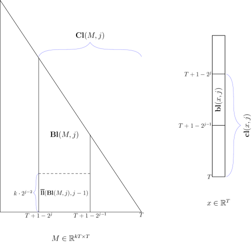
Figure 1. Notation for submatrices and sub-vectors

In our proofs, it is easier to work in terms of a matrix $B$ obtained by rescaling the entries of $M$ in such a way that

$$\inf_{y\neq 0}\frac{\left\|My\right\|_{\dagger_{\mu}(kT)}}{\left\|y\right\|_{\star_{\mu}(T)}}=\sqrt{T}\cdot\inf_{\left\|x\right\|_{2}=1}\left\|Bx\right\|_{1}.$$

Such a $k$-lower triangular matrix $B$ is obtained by setting

$$B_{(i,l),j}=\frac{M_{(i,l),j}}{\left[(T-i+1)^{1-\mu}(T-j+1)^{\mu}\right]^{1/2}}$$

for $i\geq j$ and $B_{(i,l),j}=0$ otherwise. Theorem 4.5 and Lemma 4.6 then show that for each $j$, $\overline{\textup{{ll}}}(\textup{{Bl}}(B,j),j-1)$ behaves roughly like a Dvoretzky matrix, in the sense that $\sup\frac{\left\|\overline{\textup{{ll}}}(\textup{{Bl}}(B,j),j-1)x\right\|_{1}}{\left\|x\right\|_{2}}$ is within a factor ${\Theta}(1)$ of $\inf\frac{\left\|\overline{\textup{{ll}}}(\textup{{Bl}}(B,j),j-1)x\right\|_{1}}{\left\|x\right\|_{2}}$, with probability at least $1-\exp(-\Omega(k\cdot 2^{j}))$. Corollary 4.7 strengthens this to show that with the same probability, the infimum above is not decreased substantially even if the output of $\overline{\textup{{ll}}}(\textup{{Bl}}(B,j),j-1)$ is perturbed with a vector drawn from a small dimensional subspace (namely, the range of $\textup{{Cl}}(B,j-1)$).

Lemma 4.8 then shows that the $\left\|\cdot\right\|_{1}$ norm of this perturbation itself is also preserved in the output of $\overline{\textup{{ll}}}(\textup{{Bl}}(B,j),j-1)$. Together, these results lead to Lemma 4.9 which shows, roughly speaking, that with probability $1-\exp(-\Omega(k\cdot 2^{j}))$,

$$\left\|\overline{\textup{{ll}}}(\textup{{Cl}}(B,j)\textup{{cl}}(x,j),j-1)\right\|_{1}\\ \geq\max\left\{\left\|\overline{\textup{{ll}}}(\textup{{Bl}}(B,j)\textup{{bl}}(x,j),j-1)\right\|_{1},(1-\epsilon)\left\|\overline{\textup{{ll}}}(\textup{{Cl}}(B,j-1)\textup{{cl}}(x,j-1),j-1)\right\|_{1}\right\},$$

for some small constant $\epsilon>0$. Informally, this says that the output of each trailing principal sub-matrix $\textup{{Cl}}(B,j)$ preserves both the output of its left most block $\textup{{Bl}}(B,j)$, as well as the output of the remaining trailing principal sub-matrix $\textup{{Cl}}(B,j-1)$. Underlying these results is a sequence of $\epsilon$-net arguments, which use concentration bounds on the $\ell_{1}$ norms of Gaussian vectors with independent entries of non-identical means and variances, provided in Theorems A.4 and A.7.

Finally, Theorems 4.10 and 4.11 use Lemma 4.9 in an induction to show that with probability at least $1-\exp(-\Omega(k))$,

$$\left\|Mx\right\|_{\dagger_{\mu}(kT)}\geq\tilde{\Omega}(T^{1/2-\delta})\left\|x\right\|_{\star_{\mu}(T)}$$ (13)

Equation 13 establishes that $M$ has the requisite properties at time $T$, but recall that our code requires online decoding at all times $t\leq T$. Unfortunately, we cannot take an union bound over all $t$ using eq. 13 unless we choose $k=\Omega(\log T)$, which would lead to a very low communication rate of $1/k=O(1/\log T)$ (recall that what we actually want, and achieve, is $k$ a constant).

However, there is a simple remedy if we would be willing to carry information only about a sufficiently delayed prefix of $x$. In particular, Theorems 4.10 and 4.11 also show that if $j_{0}$ is chosen so that $j_{0}=\Omega(\log\log T)$, then $M$ carries enough information about $\textup{{cl}}(x,\tau_{0},j_{0})$ (recall that this is the prefix of $x$ which ignores its last $2^{j_{0}-1}-1=\operatorname{poly}\left(\log T\right)$ entries) so that with probability at least $1-O(1/T^{2})$:

$$\left\|Mx\right\|_{\dagger_{\mu}(kT)}\geq O(T^{1/2-\delta})\left\|\textup{{cl}}(x,\tau_{0},j_{0})\right\|_{\star_{\mu}(T)}.$$

We can now indeed take a union bound over all $t\leq T$ to see that the above is true at all times $t\leq T$ with probability at least $1-O(1/T)$. However, the price we pay for this is that we cannot say anything about the most recent $\operatorname{poly}\left(\log T\right)$ characters of the message. This can be fixed by making the code systematic: the details are in Section 5.

We emphasize here that although the above discussion often refers to the total time of communication $T$, our actual construction does not assume a knowledge of $T$. In particular, the rate and error guarantees in Theorem 2.1 are achieved also at times $t$ that might be much smaller than the eventual total time $T$.

The rest of the paper is devoted to the details of the proof.

4. Progressively attenuated Gaussian matrices

Our proof of Theorem 2.1 will proceed through an analysis of a specific distribution over random $k$-lower triangular matrices. We start by recalling some results from the literature that will be used in our proofs.

4.1. Technical preliminaries

4.1.1. Operator norm of Gaussian matrices

We will use the following result on the operator norm of matrices with independent Gaussian entries.

Theorem 4.1 (Bandeira and van Handel [BvH16, Theorem 3.1]).

Let $A$ be a $n\times m$ random matrix with independent mean zero Gaussian entries such that $A_{ij}\sim\mathcal{N}(0,a_{ij}^{2})$. Then

$$\mathbb{E}\left[\left\|A\right\|_{2\rightarrow 2}\right]\leq\frac{3}{2}\left(\sigma_{1}+\sigma_{2}+10\sigma_{0}\sqrt{\log\min\left(n,m\right)}\right),$$

where

$$\sigma_{1}^{2}\mathrel{\hbox to0.0pt{\raisebox{1.29167pt}{$\cdot$}\hss}\raisebox{-1.29167pt}{$\cdot$}}=\max_{i\in[n]}\sum_{j=1}^{m}a_{ij}^{2};\;\sigma_{2}^{2}\mathrel{\hbox to0.0pt{\raisebox{1.29167pt}{$\cdot$}\hss}\raisebox{-1.29167pt}{$\cdot$}}=\max_{j\in[m]}\sum_{i=1}^{n}a_{ij}^{2};\;\sigma_{0}\mathrel{\hbox to0.0pt{\raisebox{1.29167pt}{$\cdot$}\hss}\raisebox{-1.29167pt}{$\cdot$}}=\max_{\begin{subarray}{c}i\in[n]\\ j\in[m]\end{subarray}}\left|a_{ij}\right|.$$

4.1.2. $\epsilon$-nets

We will use the following standard facts about $\epsilon$-nets for subspaces of $(\mathbb{R}^{n},\left\|\cdot\right\|_{p})$ for $p\geq 1$ (see, e. g., [FLM77]).

Fact 4.2.

Let $U$ be a subspace of $(\mathbb{R}^{n},\left\|\cdot\right\|_{p})$ of dimension at most $d$. Then, for $\epsilon\leq r$ the $\left\|\cdot\right\|_{p}$-ball (respectively, the $\left\|\cdot\right\|_{p}$-sphere) of radius $r$ in $U$ has an $\epsilon$-net in $\left\|\cdot\right\|_{p}$ of size at most $(3r/\epsilon)^{d}$.

Fact 4.3.

Let $p,q\geq 1$, and let $M$ be a $m\times n$ real matrix. If $\left\|Mx\right\|_{q}\leq c$ for all $x$ in a $\left\|\cdot\right\|_{p}$ $(1/2)$-net of the $\left\|\cdot\right\|_{p}$ sphere in $\mathbb{R}^{n}$ , then $\left\|M\right\|_{p\rightarrow q}\leq 2c$.

4.2. The distribution $\mathcal{A}_{T,k}$

We now describe the distribution on random $k$-lower triangular matrices that will be used in the proof of Theorem 2.1.

Let $T$ be a positive integer, and set $\tau=\operatorname{\textbf{{lg}}}(T)$, where

$$\operatorname{\textbf{{lg}}}(T)\mathrel{\hbox to0.0pt{\raisebox{1.29167pt}{$\cdot$}\hss}\raisebox{-1.29167pt}{$\cdot$}}=\left\lceil\lg(T+1)\right\rceil$$

is the number of bits in the canonical binary representation of $T$ . Given a rate parameter $k$, $\mathcal{A}_{T,k}$ is a distribution on $kT\times T$ $k$-lower triangular matrices, such that a matrix $M\sim\mathcal{A}_{T,k}$ is sampled as follows:

$$M((i,l),j)=\frac{1}{k\cdot\operatorname{\textbf{{lg}}}(i)^{4}}\cdot\begin{cases}0,&i<j,\\ \frac{1}{\sqrt{i-j+1}}\cdot\xi_{(i,l),j},&i\geq j.\end{cases}$$ (14)

where $i,j\in[T],l\in[k]$, and the $\xi_{(i,l),j}$ are independent standard normal random variables. Note that we divide the rows of $M$ into $T$ segments, where the $i$th segment is of size $k$, and index the rows by a pair $(i,l)$ where $i\in[T]$ denotes the segment, and $l\in[k]$ determines the offset in the segment.

Remark 4.1.

Note that the distribution $\mathcal{A}_{T,k}$ is “time-invariant” in the sense that for any $1\leq t\leq T$, the $kt\times t$ leading principal submatrix of $M$ sampled from $\mathcal{A}_{T,k}$ is also a faithful sample from $\mathcal{A}_{t,k}$.

4.3. The distribution of $\left\|M\right\|_{2\rightarrow 2}$

We begin with a short discussion of the operator norm of $M$ sampled according to $\mathcal{A}$; much of our technical work would be devoted to the study of $M^{-1}$. For the operator norm, however, the following corollary of Theorem 4.1 of Bandeira and van Handel will be sufficient for our purposes.

Lemma 4.4.

For any $\gamma\in(0,1)$ there exists a positive integer $c_{0}$ such that if $k>c_{0}$ then $M\sim\mathcal{A}_{T,k}$ satisfies $\left\|M\right\|_{2\rightarrow 2}\leq 1$ with probability at least $1-\gamma$.

Proof.

For $1\leq i\leq\operatorname{\textbf{{lg}}}(T)$, let $M(i)$ denote the submatrix of $M$ consisting of the consecutive rows from $(2^{i-1},1)$ to $(\min\left(2^{i}-1,T\right),k)$. Here, we are using the indexing scheme for rows of $M$ that was defined in eq. 14. Note that the number of non-zero columns of $M(i)$ is at most $2^{i}-1$. We now apply Theorem 4.1 to each $M(i)$. In the notation of that theorem, we have for $M(i)$

$$\sigma_{1}\leq\frac{1}{k\cdot i^{3}}\text{, }\sigma_{2}\leq\frac{1}{\sqrt{k}\cdot i^{3}}\text{ and }\sigma_{0}\leq\frac{2}{k\cdot i^{4}},$$

where we use the estimate

$$\sum_{x=1}^{n}\frac{1}{x}\leq\sum_{x=1}^{2^{\operatorname{\textbf{{lg}}}(n)}-1}\frac{1}{x}\leq\sum_{j=1}^{\operatorname{\textbf{{lg}}}(n)}\sum_{x:\operatorname{\textbf{{lg}}}(x)=j}\frac{1}{2^{j-1}}=\operatorname{\textbf{{lg}}}(n).$$

The theorem then implies that when $k\geq c$ for $c=c(\gamma)$ large enough, we have $\mathbb{E}\left[\left\|M(i)\right\|_{2\rightarrow 2}\right]\leq\frac{\gamma}{4i^{3}}$ for all $1\leq i\leq\operatorname{\textbf{{lg}}}(T)$. Thus, for $1\leq i\leq\operatorname{\textbf{{lg}}}(T)$,

$$\mathbb{P}\left[\left\|M(i)\right\|_{2\rightarrow 2}>\frac{1}{i\sqrt{2}}\right]\leq\frac{\gamma}{2i^{2}}.$$

By a union bound (and using $\sum_{i\geq 1}(1/i^{2})<2$), we get that with probability at least $1-\gamma$

$$\left\|M(i)\right\|_{2\rightarrow 2}\leq\frac{1}{i\sqrt{2}}\text{ for all $1\leq i\leq\operatorname{\textbf{{lg}}}(T)$}.$$ (15)

When the event in eq. 15 occurs, we have $\left\|M\right\|_{2\rightarrow 2}\leq 1$, since for any $x\in\mathbb{R}^{T}$ (here $x_{[l]}$ denotes the prefix of $x$ consisting of its first $l$ co-ordinates)

$$\left\|Mx\right\|_{2}^{2}=\sum_{i=1}^{\operatorname{\textbf{{lg}}}(T)}\left\|M(i)x_{[2^{i}-1]}\right\|_{2}^{2}\leq\sum_{i=1}^{\operatorname{\textbf{{lg}}}(T)}\left\|M(i)\right\|_{2\rightarrow 2}^{2}\left\|x_{[2^{i}-1]}\right\|_{2}^{2}\leq\sum_{i=1}^{\operatorname{\textbf{{lg}}}(T)}\frac{1}{2i^{2}}\left\|x_{[2^{i}-1]}\right\|_{2}^{2}\leq\sum_{j=1}^{T}x_{j}^{2}\sum_{i=\tau(j)}^{\operatorname{\textbf{{lg}}}(T)}\frac{1}{2i^{2}}\leq\left\|x\right\|_{2}^{2},$$

where the last inequality uses $\sum_{i\geq 1}(1/i^{2})<2$. ∎

4.4. Invertibility of $M$

To ease notation, we fix a $\mu\in(0,1]$ in the rest of this section, and proceed to study the robust invertibility of a matrix $M$ sampled from $\mathcal{A}_{T,k}$ with respect to the $\left\|\cdot\right\|_{\dagger_{\mu}(kT)}$ and $\left\|\cdot\right\|_{\star_{\mu}(T)}$ norms by analyzing the quantity $\inf_{y\neq 0}\frac{\left\|My\right\|_{\dagger_{\mu}(kT)}}{\left\|y\right\|_{\star_{\mu}(T)}}$. The constants appearing in the statements of the theorems appearing below therefore carry an implicit dependence upon this fixed value of $\mu$.

Our first step is to pass to standard unweighted norms via a simple reduction. Let $L$ be a $kT\times kT$ diagonal matrix with $L_{i,i}=(kT)^{(1-\mu)/2}\cdot{(kT-i+1)}^{-(1-\mu)/2}$, and let $R$ be a $T\times T$ diagonal matrix with $R_{i,i}=T^{\mu/2}\cdot(T-i+1)^{-\mu/2}$. We then have

$$\inf_{y\neq 0}\frac{\left\|My\right\|_{\dagger_{\mu}(kT)}}{\left\|y\right\|_{\star_{\mu}(T)}}=\inf_{x\neq 0}\frac{\left\|LMRx\right\|_{1}}{\left\|x\right\|_{2}}\geq\sqrt{T}\cdot\inf_{\left\|x\right\|_{2}=1}\left\|Bx\right\|_{1},$$ (16)

where the matrix $B$ is defined in terms of $M$ as follows:

$$B_{(i,l),j}=\frac{M_{(i,l),j}}{\left[(T-i+1)^{1-\mu}(T-j+1)^{\mu}\right]^{1/2}}.$$ (17)

Denote the distribution of $B$ obtained from $M\sim\mathcal{A}_{T,k}$ as $\mathcal{B}_{T,k}$. We will now study the properties of the blocks $\textup{{Bl}}(B,j)$ for $B$ sampled from this distribution in detail. We start with an investigation of their $2\rightarrow 1$ norm.

Theorem 4.5.

Let $k$ be a rate parameter such that $k\geq 1+\log 6$, and let $B\sim\mathcal{B}(T,k)$ for some positive integer $T$. Then for each $2\leq j\leq\operatorname{\textbf{{lg}}}(T)$,

$$\mathbb{P}\left[\left\|\overline{\textup{{ll}}}(\textup{{Bl}}(B,j),j-1)\right\|_{2\rightarrow 1}>\frac{256}{\sqrt{\mu}\operatorname{\textbf{{lg}}}(T)^{4}}\right]\leq\exp\left(-(k-\log 6)2^{j-1}\right).$$

Proof.

Fix $2\leq j\leq\operatorname{\textbf{{lg}}}(T)$, and let $S$ be any $1/2$-net for the unit sphere in $(R^{2^{j-1}},\left\|\cdot\right\|_{2})$. Note that we can choose $S$ so that $\left|S\right|\leq\exp\left(2^{j-1}\log 6\right)$. For ease of notation, we index the co-ordinates of any $x\in S$ from $2^{j-1}$ to $2^{j}-1$. Now, for any such $x\in S$, we have

$$\left\|\overline{\textup{{ll}}}(\textup{{Bl}}(B,j)x,j-1)\right\|_{1}=\sum_{i=1}^{2^{j-2}}\sum_{l=1}^{k}\left|X_{i,l}\right|,$$ (18)

where $X_{i,l}$ are independent mean zero normal variables with variances

$$\sigma_{i,l}^{2}=\frac{1}{k^{2}\cdot\operatorname{\textbf{{lg}}}(T-i+1)^{8}}\sum_{s=2^{j-1}}^{2^{j}-1}\frac{x_{s}^{2}}{s^{\mu}\cdot i^{1-\mu}\cdot(s-i+1)}.$$ (19)

Note that since $j\leq\operatorname{\textbf{{lg}}}(T)$, we have $T\geq 2^{j-1}$. For $1\leq i\leq 2^{j-2}$, this implies that $\operatorname{\textbf{{lg}}}(T-i+1)\geq\max(1,\operatorname{\textbf{{lg}}}(T)-1)\geq\operatorname{\textbf{{lg}}}(T)/2$, so that we have

$$\sum_{i=1}^{2^{j-2}}\sum_{l=1}^{k}\sigma_{i,l}^{2} \leq\frac{2^{8}}{k\operatorname{\textbf{{lg}}}(T)^{8}}\sum_{i=1}^{2^{j-2}}\sum_{s=2^{j-1}}^{2^{j}-1}\frac{x_{s}^{2}}{s^{\mu}\cdot i^{1-\mu}\cdot(s-i+1)}$$

$$\leq\frac{2^{11}\cdot 2^{-(1+\mu)j}\cdot{\left\|x\right\|_{2}^{2}}}{k\operatorname{\textbf{{lg}}}(T)^{8}}\cdot\sum_{i=1}^{2^{j-2}}\frac{1}{i^{1-\mu}}$$

$$\leq\frac{2^{11}\cdot 2^{-j}}{\mu k\operatorname{\textbf{{lg}}}(T)^{8}}\left\|x\right\|_{2}^{2},$$ (20)

where in the first inequality we use $0<\mu\leq 1,s\geq 2^{j-1}$ and $s-i+1\geq 2^{j-2}$, and in the second inequality the fact that $\sum_{i=1}^{N}i^{\mu-1}\leq N^{\mu}/\mu$.

We now apply Corollary A.2 to the sum in eq. 18. The number of terms $n$ is $k\cdot 2^{j-2}$, and we set the parameter $\alpha$ in Corollary A.2 to $\alpha=\frac{2^{7}}{\sqrt{\mu}\operatorname{\textbf{{lg}}}(T)^{4}\sqrt{n}}\left\|x\right\|_{2}$ to get

$$\mathbb{P}\left[\left\|\overline{\textup{{ll}}}(\textup{{Bl}}(B,j)x,j-1)\right\|_{1}>\nicefrac{{2^{7}}}{{(\sqrt{\mu}\operatorname{\textbf{{lg}}}(T)^{4})}}\left\|x\right\|_{2}\right]\leq\exp\left(-k\cdot 2^{j}\right).$$ (21)

A union bound over all $x\in S$ now yields

$$\mathbb{P}\left[\exists x\in S,\left\|\overline{\textup{{ll}}}(\textup{{Bl}}(B,j)x,j-1)\right\|_{1}>\nicefrac{{2^{7}}}{{(\sqrt{\mu}\operatorname{\textbf{{lg}}}(T)^{4})}}\left\|x\right\|_{2}\right]\leq\exp\left(-(k-\log 6)\cdot 2^{j}\right).$$ (22)

Since $S$ is a $1/2$-net, Fact 4.3 implies that $\left\|\overline{\textup{{ll}}}(\textup{{Bl}}(B,j),j-1)\right\|_{2\rightarrow 1}\leq 2^{8}/(\sqrt{\mu}\operatorname{\textbf{{lg}}}(T)^{4})$ with probability at least $1-\exp\left(-(k-\log 6)\cdot 2^{j-1}\right)$. ∎

The next lemma shows that the $\left\|\cdot\right\|_{1}$ norm of the output of $\textup{{Bl}}(B,j)$ cannot be very small.

Lemma 4.6.

There exist positive constants $c_{1},c_{2}>0$ such that the following is true. For any integer $j\geq 2$, any $k\geq c_{1}$, and any vector $y$,

$$\mathbb{P}\left[\exists x,\left\|x\right\|_{2}=1\text{ and }\right.\left.\left\|\overline{\textup{{ll}}}(\textup{{Bl}}(B,j)x+y,j-1)\right\|_{1}<c_{2}/(\operatorname{\textbf{{lg}}}(T)^{4})\right]\leq\exp\left(-c_{2}k\cdot 2^{j}\right).$$

Proof.

Let $S$ be an $\epsilon$-net for the unit sphere in $\left(\mathbb{R}^{2^{j-1}},\left\|\cdot\right\|_{2}\right)$, for an $\epsilon$ to be determined later. As in eq. 18 in the proof of Theorem 4.5, for any $x\in S$, we have

$$\left\|\overline{\textup{{ll}}}(\textup{{Bl}}(B,j)x+y,j-1)\right\|_{1}=\sum_{i=1}^{2^{j-2}}\sum_{l=1}^{k}\left|X_{i,l}+y_{i,l}\right|$$ (23)

where $X_{i,l}$ are independent mean zero normal variables with variances $\sigma_{i,l}$ as defined in eq. 19. Recall also that $\operatorname{\textbf{{lg}}}(T)-1\leq\operatorname{\textbf{{lg}}}(T-i+1)\leq\operatorname{\textbf{{lg}}}(T)$ since $i\leq 2^{j-2}$.

Since we are interested in upper bounding the probability that the above sum is small, it follows from Corollary A.6 that the worst case is $y=0$. In preparation to apply Theorem A.4 to the above sum with $y=0$, we also note that since the $\sigma_{i,l}^{2}$ are positive linear functions of the $x_{s}^{2}$ and $\left\|x\right\|_{2}=1$, $GM\left(\left(\sigma_{i,l}\right)_{\begin{subarray}{c}i\in[2^{j-2}]\\ l\in[k]\end{subarray}}\right)$ is minimized when $x=e_{s}$ for some $s\in[2^{j-1},2^{j}-1]$. We thus have

$$GM\left(\left(\sigma_{i,l}\right)_{\begin{subarray}{c}i\in[2^{j-2}]\\ l\in[k]\end{subarray}}\right) \geq\frac{1}{k\operatorname{\textbf{{lg}}}(T)^{4}}\cdot\frac{1}{\sqrt{GM\left((i^{1-\mu})_{i\in[2^{j-2}]}\right)}}\cdot\min_{s\in[2^{j-1},2^{j}-1]}\frac{1}{\sqrt{s^{\mu}GM\left((s-i+1)_{i\in[2^{j-2}]}\right)}}$$

$$\geq\frac{2^{-j/2}}{k\operatorname{\textbf{{lg}}}(T)^{4}}\min_{s\in[2^{j-1},2^{j}-1]}\frac{1}{\sqrt{s}}.$$

Applying Theorem A.4, and noting that the number of terms in the sum in eq. 23 for which the geometric mean was taken above is $k\cdot 2^{j-2}$, we now find a positive constant $c>0$ such that the following holds for all $\tau\in(0,1)$:

$$\mathbb{P}\left[\left\|\overline{\textup{{ll}}}(\textup{{Bl}}(B,j)x+y,j-1)\right\|_{1}<\frac{c\tau}{\operatorname{\textbf{{lg}}}(T)^{4}}\right]\leq\tau^{k\cdot 2^{j-2}}.$$

Taking a union bound over all $x$ in the $\epsilon$-net $S$, and then using the bound on $\left\|\overline{\textup{{ll}}}(\textup{{Bl}}(B,j),j-1)\right\|_{2\rightarrow 1}$ derived in the proof of Theorem 4.5, we then have

$$\mathbb{P}\Big{[}\exists x,\left\|x\right\|_{2}=1\text{, and }\left.\left\|\overline{\textup{{ll}}}(\textup{{Bl}}(B,j)x+y,j-1)\right\|_{1}<(c\tau-256\mu^{-1/2}\epsilon)/\operatorname{\textbf{{lg}}}(T)^{4}\right]\\ \leq\exp\left(-2^{j-1}\cdot\left[(k/2)\log(1/\tau)-\log(3/\epsilon)\right]\right)+\exp\left(-2^{j-1}\cdot(k-\log 6)\right).$$ (24)

Since $k\geq c_{1}$ for a large enough $c_{1}$, the claim now follows after choosing $\epsilon$ and $\tau$ to be appropriate constants. ∎

We now consider small dimensional perturbations to the output of $\textup{{Bl}}(B,j)$ for $j\geq 2$, and start with a corollary of Lemma 4.6.

Corollary 4.7.

There exist positive constants $C,C_{1},C_{2}>0$ such that the following is true. For any $j\geq 2$, $k\geq C_{1}$, and $V$ an arbitrary subspace of dimension at most $2(2^{j}-1)$,

$$\mathbb{P}\left[\exists x\in\mathbb{R}^{2^{j-1}},y\in V\text{ s. t. }\left\|\overline{\textup{{ll}}}(\textup{{Bl}}(B,j)x+y,j-1)\right\|_{1}\right.<\left.C\left\|x\right\|_{2}/(\operatorname{\textbf{{lg}}}(T)^{4})\right]\leq\exp\left(-C_{2}k\cdot 2^{j}\right).$$

Proof.

Let $U$ be the vector space $\left\{\overline{\textup{{ll}}}(y,j-1)\;\mathbf{|}\;y\in V\right\}$. Note that we can replace $V$ by $U$ in the statement of the corollary (i.e., if the result holds for $U$, then it also holds for $V$). We therefore restrict our attention to $U$. Note that the dimension of $U$ is no more than the dimension of $V$.

Let $c_{2}$ be as in Lemma 4.6 and define $C=c_{2}/2$. From Theorem 4.5 we know that $\left\|\overline{\textup{{ll}}}(\textup{{Bl}}(B,j),j-1)\right\|_{2\rightarrow 1}\leq 256/(\sqrt{\mu}\operatorname{\textbf{{lg}}}(T)^{4})$ with probability at least $1-\exp\left(-\Theta(k\cdot 2^{j})\right)$. Under this event we also have

$$\left\|\overline{\textup{{ll}}}(\textup{{Bl}}(B,j)x+y,j-1)\right\|_{1}\geq C/\operatorname{\textbf{{lg}}}(T)^{4}$$

whenever $\left\|x\right\|_{2}=1$ and $\left\|y\right\|_{1}>(C+256\mu^{-1/2})/\operatorname{\textbf{{lg}}}(T)^{4}$.

Therefore, let $N$ be a $\left(C/\operatorname{\textbf{{lg}}}(T)^{4}\right)$-net in $\ell_{1}$ for the $\ell_{1}$ ball of radius $(C+256\mu^{-1/2})/\operatorname{\textbf{{lg}}}(T)^{4}$ in $U$. We have $\left|N\right|\leq\exp\left(c^{\prime}2^{j}\right)$ for some $c^{\prime}>0$. Thus, applying Lemma 4.6 to each element in $N$ and then taking a union bound, we have

$$\mathbb{P}\left[\exists x\in\mathbb{R}^{2^{j-1}},y\in N\text{ s. t. }\left\|x\right\|_{2}=1\text{ and }\right.\left.\left\|\overline{\textup{{ll}}}(\textup{{Bl}}(B,j)x+y,j-1)\right\|_{1}<2C/\operatorname{\textbf{{lg}}}(T)^{4}\right]\leq\exp\left(-c^{\prime\prime}k\cdot 2^{j}\right),$$

for some positive constant $c^{\prime\prime}$ whenever $k\geq c_{1}$ for some other positive constant $c_{1}$. Using the fact that $N$ is a $(C/\operatorname{\textbf{{lg}}}(T)^{4})$-net in $\ell_{1}$ we get the claimed result. ∎

We now show that adding the output of $\textup{{Bl}}(B,j)$ does not shrink the size of the perturbation either, as long as the perturbations comes from a small dimensional space.

Lemma 4.8.

For any $\gamma\in(0,1)$ there exist positive constants $c_{1}=c_{1}(\gamma),c_{2}=c_{2}(\gamma)$ such that for any integers $j\geq 2$ and any $k>c_{1}$, the following is true. Let $V$ be an arbitrary subspace of dimension at most $2(2^{j}-1)$. Then,

$$\mathbb{P}\left[\exists x\in\mathbb{R}^{2^{j-1}},y\in V\text{ s. t. }\right.\left.\left\|\overline{\textup{{ll}}}(\textup{{Bl}}(B,j)x+y,j-1)\right\|_{1}<\gamma\left\|\overline{\textup{{ll}}}(y,j-1)\right\|_{1}\right]\leq\exp\left(-c_{2}k\cdot 2^{j}\right).$$

Proof.

From Theorem 4.5 and Corollary 4.7 we have that for some constant $c>0$, the following events occur with probability at least $1-\exp\left(-\Theta(k\cdot 2^{j})\right)$ for all large enough constant $k$:

1. $\frac{\left\|\overline{\textup{{ll}}}(\textup{{Bl}}(B,j)x,j-1)\right\|_{1}}{\left\|x\right\|_{2}}\leq 256\mu^{-1/2}/\operatorname{\textbf{{lg}}}(T)^{4}$, for all $x\neq 0$, and

2. $\left\|\overline{\textup{{ll}}}(\textup{{Bl}}(B,j)x+y,j-1)\right\|_{1}\geq c\left\|x\right\|_{2}/\operatorname{\textbf{{lg}}}(T)^{4}$ for all $x\in\mathbb{R}^{2^{j-1}},y\in V$.

We assume henceforth that both the above events occur. In particular, we have

$$\left\|\overline{\textup{{ll}}}(y,j-1)\right\|_{1}=1,\quad\left\|x\right\|_{2}\geq\frac{\gamma}{c}\cdot\operatorname{\textbf{{lg}}}(T)^{4}\qquad\implies\qquad\left\|\overline{\textup{{ll}}}(\textup{{Bl}}(B,j)x+y,j-1)\right\|_{1}\geq\gamma\left\|\overline{\textup{{ll}}}(y,j-1)\right\|_{1}.$$ (25)

Let $U$ be the vector space $\left\{\overline{\textup{{ll}}}(z,j-1)\;\mathbf{|}\;z\in V\right\}$. Now, let $N_{z}$ be an $\epsilon$-net in $\ell_{1}$ for the set $\left\{z\in U\;\mathbf{|}\;\left\|z\right\|_{1}=1\right\}$ for $\epsilon=(1-\gamma)/(1+257\mu^{-1/2})$, and $N_{x}$ and $\epsilon_{1}$-net in $\ell_{2}$ for the $\ell_{2}$-ball of radius $\frac{\gamma}{c}\cdot\operatorname{\textbf{{lg}}}(T)^{4}$ in $\mathbb{R}^{2^{j-1}-1}$ for $\epsilon_{1}=\epsilon\cdot\operatorname{\textbf{{lg}}}(T)^{4}$. $N_{z}$ and $N_{x}$ can be chosen so that $\left|N_{z}\right|\cdot\left|N_{x}\right|\leq\exp\left(c^{\prime}\cdot 2^{j}\right)$ where $c^{\prime}=c^{\prime}(\gamma)>0$. Let $\gamma^{\prime}=\gamma+(1+256\mu^{-1/2})\epsilon<1$. We now have, for any $z\in N_{z}$ and $x\in N_{x}$,

$$\left\|\overline{\textup{{ll}}}(\textup{{Bl}}(B,j)x+z,j-1)\right\|_{1}=\sum_{i=1}^{2^{j-2}}\sum_{l=1}^{k}\left|X_{i,l}+z_{i,l}\right|,$$ (26)

where, as before, $X_{i,l}$ are independent mean zero normal variables with variances $\sigma_{i,l}$ as in eq. 19. In preparation to apply Theorem A.7, we now estimate

$$\sum_{i=1}^{2^{j-2}}\sum_{\ell=1}^{k}\sigma_{i,l} \geq\frac{1}{\operatorname{\textbf{{lg}}}(T)^{4}}\sum_{i=1}^{2^{j-2}}\sqrt{\sum_{s=2^{j-1}}^{2^{j}-1}\frac{x_{s}^{2}}{s^{\mu}i^{1-\mu}(s-i+1)}}$$

$$\geq\frac{1}{\left\|x\right\|_{2}\operatorname{\textbf{{lg}}}(T)^{4}}\sum_{s=2^{j-1}}^{2^{j}-1}\frac{x_{s}^{2}}{s^{\mu/2}}\sum_{i=1}^{2^{j-2}}\frac{1}{i^{(1-\mu)/2}\sqrt{s-i+1}}$$

$$\geq\frac{\left\|x\right\|_{2}}{\operatorname{\textbf{{lg}}}(T)^{4}}2^{-j(1+\mu)/2}\sum_{i=1}^{2^{j-2}}\frac{1}{i^{(1-\mu)/2}}$$

$$\geq c_{0}\text{ for some fixed constant $c_{0}(\gamma,\mu)$}.$$

Here, the second inequality uses the concavity of the square root function, the last that $x\in N_{x}$ so that $\left\|x\right\|_{2}=\gamma\operatorname{\textbf{{lg}}}(T)^{4}/c$, and the rest are elementary estimates. Now, using the upper bound on $\sum\sigma_{i,l}^{2}$ obtained in eq. 20 (while remembering that the vector $x$ in that calculation needs to be scaled to have length $\gamma\operatorname{\textbf{{lg}}}(T)^{4}/c$ instead of $1$), we can apply Theorem A.7 to get that for some constant $c^{\prime\prime}=c^{\prime\prime}(\gamma)>0$,

$$\mathbb{P}\left[\left\|\overline{\textup{{ll}}}(\textup{{Bl}}(B,j)x,j-1)+z\right\|_{1}<\gamma^{\prime}\left\|z\right\|_{1}\right]\leq\exp\left(-c^{\prime\prime}k\cdot 2^{j}\right).$$

Taking a union bound over the product $N_{z}\times N_{x}$ of the two nets, using eq. 25 and recalling that $\gamma^{\prime}=\gamma+(1+256\mu^{-1/2})\epsilon$ and that $N_{z}$ and $N_{x}$ are $\epsilon$ and $\epsilon\cdot\operatorname{\textbf{{lg}}}(T)^{4}$ nets respectively, we deduce that for some constant $D=D(\gamma)>0$

$$\mathbb{P}\left[\exists x\in R^{2^{j-1}},z\in U\text{ s.t. }\left\|z\right\|_{1}=1\text{ and }\right.\left.\left\|\overline{\textup{{ll}}}(\textup{{Bl}}(B,j)x,j-1)+z\right\|_{1}<\gamma\right]\leq\exp\left(-Dk\cdot 2^{j}\right)$$

when $k\geq c_{1}$ for $c_{1}$ large enough. The result now follows. ∎

Combining the results of Corollaries 4.7 and 4.8, we get

Lemma 4.9.

There exists a positive constant $C$ such that for any $\gamma\in(0,1)$ there exist positive constants $c_{1}=c_{1}(\gamma),c_{2}=c_{2}(\gamma)$ such that for any integers $j\geq 2$ and any $k\geq c_{1}$, the following is true. Let $V$ be an arbitrary subspace of dimension at most $2^{j-1}-1$. Then,

$$\mathbb{P}\left[\exists x\in\mathbb{R}^{2^{j-1}},y\in V\text{ s. t. }\left\|\overline{\textup{{ll}}}(\textup{{Bl}}(B,j)x+y,j-1)\right\|_{1}\right.<\left.\max\left\{C\left\|x\right\|_{2}/\operatorname{\textbf{{lg}}}(T)^{4},\gamma\left\|\overline{\textup{{ll}}}(y,j-1)\right\|_{1}\right\}\right]\\ \leq\exp\left(-c_{2}k\cdot 2^{j}\right).$$

We are now ready to prove the main theorem of this section.

Theorem 4.10.

For any $\kappa\in(0,1)$ there exist positive constant $c_{0},c_{1}$ and $c_{2}$ such that the following is true. Let $T$ be any positive integer and set $\tau\mathrel{\hbox to0.0pt{\raisebox{1.29167pt}{$\cdot$}\hss}\raisebox{-1.29167pt}{$\cdot$}}=\operatorname{\textbf{{lg}}}(T)$. For any rate parameter $k\geq c_{1}$ and $j_{0}\in[1,\tau]$,

$$\mathbb{P}_{B\sim\mathcal{B}(T,k)}\left[\exists x\in\mathbb{R}^{T}\text{ s. t.}\left\|\overline{\textup{{ll}}}(Bx,\tau)\right\|_{1}\right.<\left.c_{0}\kappa^{\tau-j_{0}}\left\|\textup{{cl}}(x,\tau,j_{0})\right\|_{2}/\tau^{4}\right]\leq\exp\left(-c_{2}k\cdot 2^{j_{0}-1}\right).$$

Proof of Theorem 4.10.

Let $c_{0}(\kappa)$ be a fixed constant to be determined later. For $j_{0}\leq j\leq\tau$, let $\mathcal{E}_{j}$ be the event that

$$\left\|\overline{\textup{{ll}}}(\textup{{Cl}}(B,j)x,j)\right\|_{1}\geq c_{0}\kappa^{j-j_{0}}\left\|\textup{{cl}}(x,j,j_{0})\right\|_{2}/\tau^{4}\quad\forall x\in\mathbb{R}^{2^{j}-1}.$$

Corollary 4.7 (or, in the case $j_{0}=1$, a direct calculation identical to that in Lemma 4.6) shows that if $c_{0}$ is a small enough positive constant, there exist positive constants $c^{\prime},c^{\prime\prime}$ (independent of $j_{0})$ such that $\mathbb{P}\left[\lnot\mathcal{E}_{j_{0}}\right]\leq\exp\left(-c^{\prime}k2^{j_{0}-1}\right)$ for all large enough constant $k$ (to show this, one chooses the vector space $V$ in the statement of Corollary 4.7 to be $\textup{{Range}}(\textup{{Cl}}(B,j-1))$). Now, let $C>0$ be as in Lemma 4.9. We choose $c_{0}$ to be small enough so that there exists $\gamma\in\left(0,1\right)$ satisfying

$$\kappa=\frac{\gamma}{\sqrt{1+(c_{0}/C)^{2}}}.$$ (27)

The claim of the theorem then follows if there exist positive constants $c_{1},c_{2}$ such that for $k\geq c_{1}$, $\mathbb{P}\left[\lnot\mathcal{E}_{\tau}\right]\leq\exp\left(-c_{2}k2^{j_{0}-1}\right)$. We have already established this above for $j=j_{0}$. We will show now that there exists a constant $c_{2}>0$ such that for large enough constant $k$ and $j\geq 2$,

$$\mathbb{P}\left[\lnot\mathcal{E}_{j}|\mathcal{E}_{j-1}\right]\leq\exp\left(-c_{2}k\cdot 2^{j-1}\right).$$ (28)

This will establish the claim if $c_{1}$ is chosen large enough that $\exp\left(-c_{2}c_{1}\right)\leq\frac{1}{2}$, since in that case $k\geq c_{1}$ implies

$$\mathbb{P}\left[\lnot{\mathcal{E}_{\tau}}\right]\leq\mathbb{P}\left[\lnot{\mathcal{E}_{j_{0}}}\right]+\sum_{j=j_{0}+1}^{\tau}\mathbb{P}\left[\lnot\mathcal{E}_{j}|\mathcal{E}_{j-1}\right]\leq\sum_{j=j_{0}}^{\tau}\exp\left(-c_{2}k\cdot 2^{j-1}\right)\leq 2\exp\left(-c_{2}k2^{j_{0}-1}\right).$$

We now establish eq. 28. Fix $j\geq j_{0}+1$, and assume $\mathcal{E}_{j-1}$ occurs. Note that

$$\textup{{Cl}}(B,j)x=\textup{{Bl}}(B,j)\textup{{bl}}(x,j)+\textup{{Cl}}(B,j-1)\textup{{cl}}(x,j-1),$$

so that we can apply Lemma 4.9 with $V=\textup{{Range}}(\textup{{Cl}}(B,j-1))$ and $\gamma$ as chosen above to find $c_{1},c_{2}>0$ (not depending upon $j$) such that when $k\geq c_{1}$, it holds with probability at least $1-\exp\left(-c_{2}k\cdot 2^{j-1}\right)$ that

$$\frac{\left\|\overline{\textup{{ll}}}(\textup{{Cl}}(B,j)x,j)\right\|_{1}^{2}}{\left\|\textup{{cl}}(x,j,j_{0})\right\|_{2}^{2}}\geq\frac{1}{\tau^{8}}\max\Bigg{\{}C^{2}\frac{\left\|\textup{{bl}}(x,j)\right\|_{2}^{2}}{\left\|\textup{{cl}}(x,j,j_{0})\right\|_{2}^{2}},\frac{c_{0}^{2}\gamma^{2}\kappa^{2(j-j_{0})}}{\kappa^{2}}\frac{\left\|\textup{{cl}}(x,j-1,j_{0})\right\|_{2}^{2}}{\left\|\textup{{cl}}(x,j,j_{0})\right\|_{2}^{2}}\Bigg{\}}\quad\forall x\neq 0\in\mathbb{R}^{2^{j}-1}.$$ (29)

Since

$$\min_{0\leq\eta\leq 1}\max\left\{a\eta,b(1-\eta)\right\}=\frac{ab}{a+b},\text{ for all $a,b>0$,}$$

the guarantee in eq. 29 implies that for all $x\neq 0$ in $\mathbb{R}^{2^{j}-1}$.

$$\frac{\left\|\overline{\textup{{ll}}}(\textup{{Cl}}(B,j)x,j)\right\|_{1}}{\left\|\textup{{cl}}(x,j,j_{0})\right\|_{2}}\geq\frac{c_{0}\kappa^{j-1-j_{0}}}{\tau^{4}}\cdot\frac{\gamma}{\sqrt{1+(\gamma c_{0}\kappa^{j-j_{0}-1}/C)^{2}}}\geq\frac{c_{0}\kappa^{j-j_{0}}}{\tau^{4}},$$

where the last inequality uses eq. 27 and the fact that $\gamma,\kappa\leq 1$. We thus have $\mathbb{P}\left[\mathcal{E}_{j}|\mathcal{E}_{j-1}\right]\geq 1-\exp\left(-c_{2}k\cdot 2^{j-1}\right)$, as required. ∎

We now use the information about $B$ derived above to show that $M$ comes very close to satisfying the conditions asked of an encoding matrix in Theorem 2.1. In particular, Corollary 4.11 implies that $M$ satisfies these constraints at any given fixed time $T$. Corollary 4.12 then shows that encoding using $M$ actually satisfies, at each time $t$ up to the total time $T$ for which communication lasts, a slightly weaker set of conditions which allow for the decoding of all but a $\operatorname{poly}\left(\log t\right)$ sized suffix of the signal. Finally, we obtain the full statement of Theorem 2.1 in Section 5 by slightly modifying $M$ to handle the suffix differently.

Corollary 4.11 (Invertibility of $M$).

For any $\delta\in(0,\frac{1}{2})$, there exist constants $c_{0},c_{1},c_{2}$ such that the following is true. Let $T$ be a fixed integer, and let $\tau=\operatorname{\textbf{{lg}}}(T)$. Let $k\geq c_{1}$ be a rate parameter. Then, for $M$ sampled according to $\mathcal{A}_{T,k}$, we have

$$\mathbb{P}\left[\exists x\in\mathbb{R}^{T}\text{ s.t. }\left\|Mx\right\|_{\dagger_{\mu}(kT)}\right.<\left.c_{0}2^{\delta j_{0}}2^{\tau(1/2-\delta)}\left\|\textup{{cl}}(x,\tau,j_{0})\right\|_{\star_{\mu}(T)}/\tau^{4}\right]\leq\exp\left(-c_{2}k\cdot 2^{j_{0}-1}\right)$$

for all $1\leq j_{0}\leq\tau$. Here, for the purposes of computing the $\left\|\cdot\right\|_{\star_{\mu}(T)}$-norm, $\textup{{cl}}(x,\tau,j_{0})$ is seen as a vector in $\mathbb{R}^{T}$ whose last $2^{j_{0}-1}-1$ coordinates are $0$.

Proof.

Using the same calculation as in eq. 16, we see that if $M\sim\mathcal{A}_{T,k}$, and $B$ is constructed from $M$ as defined in eq. 17, then $B\sim\mathcal{B}_{T,k}$ and

$$\inf\frac{\left\|Mx\right\|_{\dagger_{\mu}(kT)}}{\left\|\textup{{cl}}(x,\tau,j_{0})\right\|_{\star_{\mu}(T)}}\geq 2^{\tau/2-1}\inf\frac{\left\|By\right\|_{1}}{\left\|\textup{{cl}}(y,\tau,j_{0})\right\|_{2}}.$$ (30)

Given $\delta\in\left(0,\frac{1}{2}\right)$, we choose $\kappa=2^{-\delta}$. After applying Theorem 4.10 with this value of $\kappa$ and using eq. 30, we then find positive constants $c_{0},c_{1},c_{2}$ (depending upon $\kappa$) such that when $k\geq c_{1}$, the matrix $M$ satisfies

$$\left\|Mx\right\|_{\dagger_{\mu}(kT)}\geq c_{0}2^{\delta j_{0}+\tau(1/2-\delta)}\left\|\textup{{cl}}(x,t,j_{0})\right\|_{\star_{\mu}(T)}/\tau^{4}\;\forall x$$

with probability at least $1-\exp\left(-c_{2}k\cdot 2^{j_{0}-1}\right)$. ∎

Corollary 4.12 (Invertibility of principal submatrices of $M$).

For any $\delta\in(0,\frac{1}{2})$, there exist constants $c_{0},c_{1}$ such that the following is true. Let $T$ be a positive integer, and set $\tau\mathrel{\hbox to0.0pt{\raisebox{1.29167pt}{$\cdot$}\hss}\raisebox{-1.29167pt}{$\cdot$}}=\operatorname{\textbf{{lg}}}(T)$, $j_{0}(n)\mathrel{\hbox to0.0pt{\raisebox{1.29167pt}{$\cdot$}\hss}\raisebox{-1.29167pt}{$\cdot$}}=\left\lceil\frac{4\operatorname{\textbf{{lg}}}(\operatorname{\textbf{{lg}}}(n))}{\delta}\right\rceil=\Theta(\log\log n)$. Then, for any rate parameter $k\geq c_{1}$, there exists a $k$-lower triangular matrix $M$ satisfying the following conditions. (Here, for $1\leq n\leq T$ and a $k$-lower triangular matrix $A$, $A_{n}$ denotes the $k$-lower triangular matrix obtained by taking the first $n$ columns of $A$ and the first $kn$ rows).

1. Submatrices of $M$ have small operator norm: $\left\|M_{n}\right\|_{2\rightarrow 2}\leq 1$ for $1\leq n\leq T$.

2. Submatrices of $M$ are robustly invertible with respect to the past: for $1\leq n\leq T$,

   $$\left\|M_{n}x\right\|_{\dagger_{\mu}(kn)}\geq{c_{0}n^{(1/2-\delta)}}\left\|\textup{{cl}}(x,\operatorname{\textbf{{lg}}}(n),j_{0}(n))\right\|_{\star_{\mu}(n)}.$$

   for all $x\in\mathbb{R}^{n}$.

Proof.

Let $M\sim\mathcal{A}_{T,k}$. We will show that when $k\geq c_{1}$ for $c_{1}$ large enough, then $M$ satisfies both the above conditions with positive probability. We start by noting that Lemma 4.4 implies that item 1 is satisfied with probability at least $\frac{1}{2}$, as long as $c_{1}$ is large enough. We now turn to item 2.

Each sub-matrix $M_{n}$ of $M$ is a sample from $\mathcal{A}_{n,k}$. From Corollary 4.11, we therefore find constants $c_{0},c_{1}^{\prime}$ and $c_{2}^{\prime}$ such that as long as $k\geq c_{1}^{\prime}$, we have

$$\mathbb{P}\left[\exists x\in\mathbb{R}^{n},\left\|M_{n}x\right\|_{\dagger_{\mu}(kn)}\right.<\left.\frac{c_{0}2^{\delta j_{0}(n)}2^{\operatorname{\textbf{{lg}}}(n)(1/2-\delta)}}{\operatorname{\textbf{{lg}}}(n)^{4}}\left\|\textup{{cl}}(x,\operatorname{\textbf{{lg}}}(n),j_{0}(n))\right\|_{\star_{\mu}(n)}\right]\leq e^{-c_{2}^{\prime}k2^{j_{0}(n)}}\leq e^{-c_{2}^{\prime}k\operatorname{\textbf{{lg}}}(n)^{8}},$$ (31)

where the last inequality uses the value of $j_{0}$. (Note that, strictly speaking, we can only apply Corollary 4.11 when $j_{0}(n)\leq\operatorname{\textbf{{lg}}}(n)$. However, when $j_{0}(n)>\operatorname{\textbf{{lg}}}(n)$, eq. 31 is vacuously satisfied since in that case, $\textup{{cl}}(x,\operatorname{\textbf{{lg}}}(n),j_{0}(n))$ is an empty vector for all $x\in\mathbb{R}^{n}$.) Now, when $k\geq c_{1}$ where $c_{1}$ is chosen to be large enough that $c_{2}^{\prime}c_{1}\geq 10$ and $c_{1}\geq c_{1}^{\prime}$, we can substitute the value of $j_{0}(n)$ in eq. 31 to find that for all $1\leq n\leq T$

$$\mathbb{P}\left[\exists x\in\mathbb{R}^{n},\left\|M_{n}x\right\|_{\dagger_{\mu}(kn)}\right.<\left.{c_{0}2^{\operatorname{\textbf{{lg}}}(n)(1/2-\delta)}}\left\|\textup{{cl}}(x,\operatorname{\textbf{{lg}}}(n),j_{0}(n))\right\|_{\star_{\mu}(n)}\right]\leq e^{-10\operatorname{\textbf{{lg}}}(n)^{8}}\leq\frac{1}{10n^{2}}.$$

Taking a union bound over $1\leq n\leq T$ and using $\sum_{n\geq 1}(1/n^{2})<2$, we now see that $M$ satisfies both conditions with probability at least $\frac{1}{2}-\frac{1}{5}=\frac{3}{10}$. ∎

5. The encoding matrix

Corollary 4.12 already contains most of the information necessary for the construction of our encoding matrix. Indeed, the matrix $M$ guaranteed there can already decode all but the last $\operatorname{poly}\left(\log t\right)$ entries at any time $t$ with the required guarantee. To get the final guarantee, we only need to make our encoding systematic by including a copy of the input symbols. More precisely, given a $k$-lower triangular matrix of the form guaranteed by Corollary 4.12, we construct a $(k+1)$-lower triangular matrix $C$ which at time $t$ produces the $k$ symbols that would have been output by $M$, followed by the current input $x_{t}$. In symbols, this means that entries of $C$ can be written as follows (we use again the block notation for row indices of $k$-lower triangular matrices introduced in Section 2):

$$C_{(i,l),j}=\begin{cases}M_{(i.l),j}&\text{ when $1\leq l\leq k$,}\\ 1&\text{ when $l=k+1$, and}\\ 0&\text{otherwise}\end{cases}$$ (32)

We note the following simple consequences of this definition:

1. Let $y=Mx$ for $x\in\mathbb{R}^{T}$. Then

   $$\left\|Cx\right\|_{\dagger_{\mu}((k+1)T)} =\sum_{\begin{subarray}{c}1\leq i\leq T\\ 1\leq l\leq k\end{subarray}}\left|y_{(i,l)}\right|\left(\frac{(k+1)T}{(k+1)(T-i+1)-l+1}\right)^{(1-\mu)/2}$$

   $$\qquad\qquad+\sum_{i=1}^{T}\left|x_{i}\right|\left(\frac{(k+1)T}{(k+1)(T-i+1)-k}\right)^{(1-\mu)/2}$$

   $$\geq\frac{\left\|y\right\|_{\dagger_{\mu}(kT)}}{3}+\sum_{i=1}^{T}\left|x_{i}\right|\left(\frac{T}{T-i+1}\right)^{(1-\mu)/2}.$$ (33)

2. For every $x\in\mathbb{R}^{T}$,

   $$\left\|Cx\right\|_{2}^{2}={\left\|Mx\right\|_{2}^{2}+\left\|x\right\|_{2}^{2}}.$$ (34)

We can now prove Theorem 2.1 which we restate here for easy reference.

Theorem (The encoding matrix, restatement of Theorem 2.1).

For any $\mu\in(0,1]$ and $\delta\in(0,\frac{1}{2})$, there exist constants $c,c_{1}$ such that the following is true. Let $T\geq 3$ be any integer. For a rate parameter $k$ satisfying $k\geq c_{1}$, there exists a matrix $\mathcal{C}$ satisfying the following conditions. (Here, for $1\leq n\leq T$ and a $k$-lower triangular matrix $A$, $A_{n}$ denotes the leading principal sub-matrix of $A$ consisting of its first $n$ columns and $kn$ rows).

1. Submatrices of $\mathcal{C}$ have small operator norm: $\left\|\mathcal{C}_{n}\right\|_{2\rightarrow 2}\leq 1$ for $1\leq n\leq T$.

2. Submatrices of $\mathcal{C}_{n}$ are robustly invertible: for $1\leq n\leq T$,

   $$\left\|\mathcal{C}_{n}x\right\|_{\dagger_{\mu}(kn)}\geq cn^{(1/2-\delta)}\left\|x\right\|_{\star_{\mu}(n)}\text{ for all $x\in\mathbb{R}^{n}$}.$$

Proof.

Applying Corollary 4.12 with $\mu$ and $\delta$, we obtain $c_{0},c_{1},j_{0}$ and a $k$-lower triangular matrix $M$ (for a $k\geq c_{1}$) as in the corollary. We define the $k+1$-lower triangular matrix $C$ using $M$ as done in eq. 32 above, and set $\mathcal{C}=\frac{1}{\sqrt{2}}C$. Item 1 now follows from item 1 and eq. 34.

For item 2, we use eq. 33 followed by item 2 of Corollary 4.12 to get (with $c^{\prime}\mathrel{\hbox to0.0pt{\raisebox{1.29167pt}{$\cdot$}\hss}\raisebox{-1.29167pt}{$\cdot$}}=c_{0}/3)$

$$\sqrt{2}\left\|\mathcal{C}_{n}x\right\|_{\dagger_{\mu}(kn)}\geq c^{\prime}n^{(1/2-\delta)}\left\|\textup{{cl}}(x,\operatorname{\textbf{{lg}}}(n),j_{0}(n))\right\|_{\star_{\mu}(n)}+\sum_{i=1}^{n}\left(\frac{n}{n-i+1}\right)^{(1-\mu)/2}\left|x_{i}\right|,\text{ for all $x\in\mathbb{R}^{n}$,}$$ (35)

where $\operatorname{\textbf{{lg}}}(n)\mathrel{\hbox to0.0pt{\raisebox{1.29167pt}{$\cdot$}\hss}\raisebox{-1.29167pt}{$\cdot$}}=\left\lceil\lg(n+1)\right\rceil$, and $j_{0}$ is as in Corollary 4.12 and satisfies $j_{0}(n)=O(\log\log n)$. We now estimate the second term as follows:

$$\sum_{i=1}^{n}\left(\frac{n}{n-i+1}\right)^{(1-\mu)/2}\left|x_{i}\right| \geq\sum_{i=n-2^{j_{0}(n)}+2}^{n}\frac{\sqrt{n}}{\sqrt{n-i+1}}\cdot\left(\frac{n-i+1}{n}\right)^{\mu/2}\left|x_{i}\right|$$

$$\geq\frac{\sqrt{n}}{O(\operatorname{poly}\left(\log n\right))}\sqrt{\sum_{i=n-2^{j_{0}(n)}+2}^{n}\left(\frac{n-i+1}{n}\right)^{\mu}\left|x_{i}\right|^{2}}$$

$$\geq c^{\prime\prime}n^{(1/2-\delta)}\left\|\textup{{cl}}(x,j_{0}(n)-1)\right\|_{\star_{\mu}(n)},$$

for some fixed positive constant $c^{\prime\prime}=c^{\prime\prime}(\delta)$. Item 2 now follows by substituting this into eq. 35 and using the fact that

$$\left\|\textup{{cl}}(x,j_{0}(n)-1)\right\|_{\star_{\mu}(n)}+\left\|\textup{{cl}}(x,\operatorname{\textbf{{lg}}}(n),j_{0}(n))\right\|_{\star_{\mu}(n)}\\ \geq\sqrt{\left\|\textup{{cl}}(x,j_{0}(n)-1)\right\|_{\star_{\mu}(n)}^{2}+\left\|\textup{{cl}}(x,\operatorname{\textbf{{lg}}}(n),j_{0}(n))\right\|_{\star_{\mu}(n)}^{2}}=\left\|x\right\|_{\star_{\mu}(n)}.\qed$$

6. Comparing the online and block settings: A lower bound

As noted in the introduction, when compared with the block coding setting, we lose an extra $\Theta(t^{\delta})$ factor in the robust invertibility guarantee in the online setting. A natural question therefore is whether it is possible to get rid of this loss and obtain a guarantee as strong as the block coding setting (eq. 7) in the online setting as well. We now prove Theorem 2.2, which was stated in the introduction as a partial answer to this question. We restate the theorem here for ease of reference.

Theorem 6.1.

Fix $\mu\in(0,1]$, $c_{0}>0$ and a positive integer $k$. There exists a constant $\tau=\tau(\mu,c_{0},k)$ such that the following is true. If $\mathcal{C}$ is a $kT\times T$ $k$-lower triangular matrix such that for all $t\in[T]$ the submatrix $\mathcal{C}_{t}$ of $\mathcal{C}$ satisfies

$$\left\|\mathcal{C}_{t}x\right\|_{\dagger_{\mu}(kt)}\geq{c_{0}t^{1/2}}\left\|x\right\|_{\star_{\mu}(t)}\text{ for all $x\in\mathbb{R}^{t}$},$$ (36)

then there exists a non-zero $x\in\mathbb{R}^{T}$ for which

$$\left\|\mathcal{C}x\right\|_{2}^{2}\geq\tau\left\|x\right\|_{2}^{2}\sum_{i=1}^{T}\frac{1}{i}\geq\left(\tau\log T\right)\cdot\left\|x\right\|_{2}^{2}.$$

In particular, $x$ can be taken to be the unit pulse at time $1$.

Proof.

When $x=e_{1}$ is the unit pulse at time $1$, we have $\left\|x_{[t]}\right\|_{\star_{\mu}(t)}=1$ for all $\mu\in(0,1]$ and $1\leq t\leq T$. Let $z\in\mathbb{R}^{kT}$ be the vector such that $z_{i}\mathrel{\hbox to0.0pt{\raisebox{1.29167pt}{$\cdot$}\hss}\raisebox{-1.29167pt}{$\cdot$}}=\left|\mathcal{C}_{i,1}\right|$. Then, for $x=e_{1}$, we have

$$\left\|\mathcal{C}x\right\|_{2} =\left\|z\right\|_{2}\text{, and }$$

$$\left\|\mathcal{C}_{t}x_{[t]}\right\|_{\dagger_{\mu}(kt)} =\sum_{i=1}^{kt}z_{i}\cdot\left(\frac{kt}{kt-i+1}\right)^{(1-\mu)/2}.$$

It therefore follows that when the guarantees of eq. 36 are enforced, the objective value of the following convex program is a lower bound on $\left\|\mathcal{C}e_{1}\right\|_{2}$:

$$\min \qquad\left\|z\right\|_{2}^{2}$$ (37)

subject to $$\qquad\sum_{i=1}^{kt}z_{i}f_{it} \geq\gamma_{t}\text{, } 1\leq t\leq T$$

$$\qquad z_{i} \geq 0,\text{ } 1\leq i\leq kT.$$

Here

$$\gamma_{t}\mathrel{\hbox to0.0pt{\raisebox{1.29167pt}{$\cdot$}\hss}\raisebox{-1.29167pt}{$\cdot$}}=\frac{c_{0}t^{\mu/2}}{k^{(1-\mu)/2}}\text{, and }f_{it}\mathrel{\hbox to0.0pt{\raisebox{1.29167pt}{$\cdot$}\hss}\raisebox{-1.29167pt}{$\cdot$}}=\frac{1}{(kt-i+1)^{(1-\mu)/2}}.$$

We will lower bound the objective value of this program by providing a feasible solution to its dual program. The dual program is given as

$$\sup \qquad g(\lambda,\nu)$$ (38)

subject to $$\qquad\lambda_{i} \geq 0\text{, } 1\leq i\leq T$$

$$\qquad\nu_{i} \geq 0,\text{ } 1\leq i\leq kT$$

where

$$g(\lambda,\nu)\mathrel{\hbox to0.0pt{\raisebox{1.29167pt}{$\cdot$}\hss}\raisebox{-1.29167pt}{$\cdot$}}=\inf_{z\in\mathbb{R}^{kT}}\left\|z\right\|_{2}^{2}-\sum_{t=1}^{T}\lambda_{t}\left(\sum_{i=1}^{kt}z_{i}f_{it}-\gamma_{t}\right)-\sum_{i=1}^{kT}\nu_{i}z_{i}.$$

The expression to be minimized in the definition of $g$ is a convex function of $z$, and hence we can perform the minimization by equating the gradient to $0$. This yields

$$g(\lambda,\nu)=\sum_{t=1}^{T}\lambda_{t}\gamma_{t}-\frac{1}{4}\sum_{t=1}^{kT}\Lambda_{i}^{2}-\frac{1}{4}\sum_{i=1}^{kT}\nu_{i}^{2}-\frac{1}{2}\sum_{t=1}^{kT}\Lambda_{t}\nu_{t},$$ (39)

where, for $1\leq i\leq kT$,

$$\Lambda_{i}\mathrel{\hbox to0.0pt{\raisebox{1.29167pt}{$\cdot$}\hss}\raisebox{-1.29167pt}{$\cdot$}}=\sum_{t=\left\lceil i/k\right\rceil}^{T}\lambda_{t}f_{it}=\sum_{t=\left\lceil i/k\right\rceil}^{T}\frac{\lambda_{t}}{(kt-i+1)^{(1-\mu)/2}}.$$

Note that when $\lambda$ and $\nu$ are non-negative, $g$ is non-increasing in the $\nu_{i}$, and hence we can set $\nu_{i}=0$ (for $1\leq i\leq kT$) without changing the optimal value of the program in (38). We now consider the following dual feasible solution:

$$\lambda_{t} =\frac{a_{0}}{t^{1+\mu/2}} 1\leq t\leq T$$ for , and (40)

$$\nu_{i} =0 1\leq i\leq kT$$ for ,

where $a_{0}$ is a positive constant to be chosen later. To lower bound the dual objective value, we now upper bound the $\Lambda_{i}$ given this choice of the $\lambda_{t}$. For positive integers $i$ and $j$ such that $1\leq j\leq T$ and $k(j-1)+1\leq i\leq kj$, we have

$$\Lambda_{i} =a_{0}\sum_{t=j}^{T}\frac{1}{t^{1+\mu/2}(kt-i+1)^{(1-\mu)/2}}$$

$$\leq a_{0}\sum_{t=j}^{T}\frac{1}{t^{1+\mu/2}\cdot(kt-kj+1)^{(1-\mu)/2}}$$

$$\leq\frac{a_{0}}{j^{1+\mu/2}}+\frac{a_{0}}{k^{(1-\mu)/2}}\sum_{t=1}^{T-j}\frac{1}{(t+j)^{1+\mu/2}\cdot t^{(1-\mu)/2}}.$$ (41)

The last term above can also be shown to be $O(\sqrt{j})$, as follows:

$$\sum_{t=1}^{T-j}\frac{1}{(t+j)^{1+\mu/2}\cdot t^{(1-\mu)/2}} \leq\sum_{t=1}^{\infty}\frac{1}{(t+j)^{1+\mu/2}\cdot t^{(1-\mu)/2}}$$

$$=\sum_{l=1}^{\infty}\sum_{t=(l-1)j+1}^{lj}\frac{1}{(t+j)^{1+\mu/2}\cdot t^{(1-\mu)/2}}$$

$$\leq\sum_{l=1}^{\infty}\frac{1}{(lj)^{1+\mu/2}}\sum_{t=(l-1)j+1}^{lj}\frac{1}{t^{(1-\mu)/2}}$$

$$\leq\frac{2}{1+\mu}\sum_{l=1}^{\infty}\frac{j^{(1+\mu)/2}}{(lj)^{1+\mu/2}}\cdot\left(l^{(1+\mu)/2}-(l-1)^{(1+\mu)/2}\right)$$

$$\leq\frac{2}{1+\mu}\cdot\frac{1}{\sqrt{j}}\sum_{l=1}^{\infty}\frac{1}{l^{1+\mu/2}}\leq\frac{2(2+\mu)}{\mu(1+\mu)}\cdot\frac{1}{\sqrt{j}}.$$

Here, the third and the last inequalities use Fact 6.2 (note that $\mu>0$, so only the case $\alpha\neq 1$ of Fact 6.2 is used), and the fourth uses the fact that when $\beta\in(0,1]$ and $n$ is a non-negative integer, $(n+1)^{\beta}-n^{\beta}\leq 1$. Plugging the above estimate into eq. 41, we get that when $j$ is a positive integer such that $k(j-1)+1\leq i\leq kj$,

$$\Lambda_{i}\leq\frac{a_{0}c^{\prime}}{\sqrt{j}},$$

where $c^{\prime}=c^{\prime}(\mu,k)\mathrel{\hbox to0.0pt{\raisebox{1.29167pt}{$\cdot$}\hss}\raisebox{-1.29167pt}{$\cdot$}}=1+\frac{2(2+\mu)}{\mu(1+\mu)\cdot k^{(1-\mu)/2}}$. Thus, at the feasible solution in eq. 40, the dual objective value is

$$g(\lambda,\mathbf{0}) =\sum_{t=1}^{T}\lambda_{t}\gamma_{t}-\frac{1}{4}\sum_{i=1}^{kT}\Lambda_{i}^{2}$$

$$=\frac{a_{0}c_{0}}{k^{(1-\mu)/2}}\sum_{t=1}^{T}\frac{1}{t}-\frac{1}{4}\sum_{i=1}^{kT}\Lambda_{i}^{2}$$

$$\geq a_{0}\left(\frac{c_{0}}{k^{(1-\mu)/2}}-\frac{ka_{0}{c^{\prime}}^{2}}{4}\right)\sum_{t=1}^{T}\frac{1}{t},$$

where the last inequality uses the above estimate on $\Lambda_{i}$. Thus, by choosing $a_{0}=a_{0}(\mu,c_{0},k)$ to be $\frac{2c_{0}}{k^{(3-\mu)/2}c^{\prime 2}}$, we find that there exists a positive constant $\tau=\tau(\mu,c_{0},k)$ such that the dual objective value is at least $\tau\sum_{t=1}^{T}\frac{1}{t}$. By weak duality, this is also a lower bound on the objective value of the primal program in (37). By the discussion preceding (37), this completes the proof. ∎

The proof of Theorem 6.1 uses the following elementary estimate.

Fact 6.2.

Let $a<b$ be positive integers and $\alpha$ a positive real number. Then,

$$\sum_{i=a+1}^{b}i^{-\alpha}\leq\int_{a}^{b}x^{-\alpha}dx=\begin{cases}\frac{b^{1-\alpha}-a^{1-\alpha}}{1-\alpha}&\textup{when $\alpha\neq 1$,}\\ \log(b/a)&\textup{when $\alpha=1$.}\end{cases}$$

Appendix A $\left\|\cdot\right\|_{1}$-norms of non-uniform Gaussian vectors

In this section we collect concentration bounds for the $\left\|\cdot\right\|_{1}$-norms of Gaussian vectors with independent but not identically distributed entries. The bounds here are adaptations of standard arguments and results in the literature on Gaussian concentration to our setting.

We begin with the following elementary fact and a consequence, and then proceed to bounds for the lower tail of the $\left\|\cdot\right\|_{1}$ norm of Gaussian vectors with independent but not identically distributed entries (in Theorems A.4 and A.7).

Fact A.1 (Gaussian tail).

If $X\sim\mathcal{N}(0,\sigma^{2})$, then for $t>0$,

$$\mathbb{P}\left[X\geq t\right]=\frac{1}{\sqrt{2\pi\sigma^{2}}}\int\limits_{t}^{\infty}\exp\left(-x^{2}/(2\sigma^{2})\right)dx<\frac{\sigma}{t\cdot\sqrt{2\pi}}\exp\left(-\frac{t^{2}}{2\sigma^{2}}\right).$$

Corollary A.2 (Upper tail of the $\left\|\cdot\right\|_{1}$-norm).

Let $X\sim\mathcal{N}\left(0,\mathop{\mathrm{diag}}\left((\sigma_{i}^{2})_{i=1}^{n}\right)\right)$. Then, for any $t>0$ and $c>0$, we have

$$\mathbb{P}\left[\left\|X\right\|_{1}>t\right]\leq\exp\left(-ct+n\log 2+\frac{c^{2}}{2}\sum_{i=1}^{n}\sigma_{i}^{2})\right).$$

In particular, choosing $c=\frac{t}{\sum_{i=1}^{n}\sigma_{i}^{2}}$ and then $t=\alpha\sqrt{n}$, we have

$$\mathbb{P}\left[\left\|X\right\|_{1}>\alpha\sqrt{n}\right]\leq\exp\left(-n\left(\frac{\alpha^{2}}{2\sum_{i=1}^{n}\sigma_{i}^{2}}-\log 2\right)\right).$$

Proof.

For $Y\sim\mathcal{N}(0,\sigma^{2})$, we have, for any $c>0$, $\mathbb{E}\left[\exp(c\left|Y\right|)\right]\leq 2\exp(c^{2}\sigma^{2}/2)$. Thus we have, for any $c>0$,

$$\mathbb{P}\left[\left\|X\right\|_{1}>t\right]=\mathbb{P}\left[\exp(c\left\|X\right\|_{1})>\exp(ct)\right]\leq\exp(-ct)\prod_{i=1}^{n}\mathbb{E}\left[\exp(c\left|X_{i}\right|)\right]\leq\exp\left(-ct+n\log 2+\frac{c^{2}}{2}\sum_{i=1}^{n}\sigma_{i}^{2}\right).\qed$$

A.1. The lower tail of the $\left\|\cdot\right\|_{1}$-norm

We now state two concentration results for the lower tail of the $\ell_{1}$ norm of Gaussian vectors with independent but not identically distributed entries. The first (Theorem A.4) deals with the lower tail for mean $0$ vectors (in other words, this is an upper bound on small-ball probability), while the second (Theorem A.7) considers the concentration around the $\ell_{1}$ norm of the mean for vectors with non-zero mean.

Lemma A.3.

Let $X\sim\mathcal{N}\left(0,\mathop{\mathrm{diag}}\left((\sigma_{i}^{2})_{i=1}^{n}\right)\right)$. Then, for any $t>0$ and $c>0$, we have

$$\mathbb{P}\left[\left\|X\right\|_{1}<t\right]\leq\exp(ct+\sum_{i=1}^{n}\nu(c^{2}\sigma_{i}^{2})),$$

where for $x\geq 0$,

$$\nu(x)\mathrel{\hbox to0.0pt{\raisebox{1.29167pt}{$\cdot$}\hss}\raisebox{-1.29167pt}{$\cdot$}}=\frac{x}{2}-\frac{1}{2}\log\frac{\pi}{2}+\log\int\limits_{\sqrt{x}}^{\infty}\exp(-t^{2}/2)dt\leq\frac{1}{2}\min\left\{0,-\log\frac{\pi x}{2}\right\}.$$

Proof.

Let $X=(X_{1},X_{2},\dots,X_{n})$ where $X_{i}\sim\mathcal{N}(0,\sigma_{i}^{2})$. For any $c>0$, we have

$$\mathbb{P}\left[\left\|X\right\|_{1}<t\right]=\mathbb{P}\left[\exp\left(-c\left\|X\right\|_{1}\right)>\exp(-ct)\right]\leq\exp(ct)\cdot\prod_{i=1}^{n}\mathbb{E}\left[\exp\left(-c\left|X_{i}\right|\right)\right].$$ (42)

The first claim now follows since for $Y\sim\mathcal{N}(0,\sigma^{2})$, we have

$$\mathbb{E}\left[\exp\left(-c\left|Y\right|\right)\right] =\sqrt{\frac{2}{\pi\sigma^{2}}}\int\limits_{0}^{\infty}\exp\left(-cy-\frac{y^{2}}{2\sigma^{2}}\right)dy$$

$$=\sqrt{\frac{2}{\pi}}\exp(c^{2}\sigma^{2}/2)\int\limits_{0}^{\infty}\exp\left(-(z+c\sigma)^{2}/2\right)dz$$

$$=\sqrt{\frac{2}{\pi}}\exp(c^{2}\sigma^{2}/2)\int\limits_{c\sigma}^{\infty}\exp\left(-z^{2}/2\right)dz$$

$$=\exp\left(\nu(c^{2}\sigma^{2})\right).$$

The definition of $\nu$ implies that $\nu(x)\leq 0$ for all positive $x$. Now, using Fact A.1, we have

$$\nu(x)\leq-\frac{1}{2}\log\left(\frac{\pi}{2}\right)+\frac{x}{2}+\log\left(\frac{1}{\sqrt{x}}\exp\left(-x/2\right)\right)=-\frac{1}{2}\log\left(\frac{\pi x}{2}\right)\text{, for all $x\geq 0$.}$$

Thus, we obtain $\nu(x)\leq\frac{1}{2}\min\left\{0,-\log\frac{\pi x}{2}\right\}$. ∎

Theorem A.4 (Lower tail of the $\left\|\cdot\right\|_{1}$-norm).

There exists a positive constant $\gamma$ such that the following is true. Let $X\sim\mathcal{N}\left(0,\mathop{\mathrm{diag}}\left((\sigma_{i}^{2})_{i=1}^{n}\right)\right)$, $S$ an arbitrary subset of $[n]$. Define $G\mathrel{\hbox to0.0pt{\raisebox{1.29167pt}{$\cdot$}\hss}\raisebox{-1.29167pt}{$\cdot$}}=GM\left(\left(\sigma_{i}\right)_{i\in S}\right)$ to be the geometric mean of the $\sigma_{i}$ for $i\in S$. Then, for all $\tau\geq 0$ and

$$t\leq\tau\gamma G|S|$$

we have

$$\mathbb{P}\left[\left\|X\right\|_{1}<t\right]\leq\left(\tau\right)^{|S|}.$$

In particular, given $\alpha$, if there exists a set $S$ for which $G\geq\alpha/|S|$, then for all $\tau\geq 0$,

$$\mathbb{P}\left[\left\|X\right\|_{1}<\tau\gamma\cdot\alpha\right]\leq\tau^{|S|}.$$

Proof.

Set $\gamma=\sqrt{\pi/2}/e$. We now use Lemma A.3 and the upper bound on the function $\nu$ defined there, after exercising our choice for $c$ by setting $c=|S|/t$. We then have

$$\mathbb{P}\left[\left\|X\right\|_{1}<t\right] \leq\exp\big{(}ct+|S|\log(\sqrt{2/\pi})-|S|\log c-|S|\log G\big{)}$$

$$=\exp\left(|S|\left(-\log\gamma-\log|S|+\log t-\log|G|\right)\right)$$

$$=\left(\frac{t}{\gamma G|S|}\right)^{|S|}.$$

Substituting $t=\tau\gamma|G|S$, we get the claimed result. ∎

The standard fact below shows that it is sufficient to consider mean $0$ vectors in the setting of Theorem A.4. We include a proof for completeness.

Fact A.5 (Stochastic domination of absolute values of Gaussians).

Let $X\sim\mathcal{N}(0,\sigma^{2})$. Then the random variable $\left|a+X\right|$ stochastically dominates the random variable $\left|b+X\right|$ whenever $\left|a\right|>\left|b\right|$.

Proof.

Without loss of generality, we assume $\sigma=1$ and $a>b>0$. Now for any fixed $y\geq 0$ and $x\in[b,a]$, we have

$$\mathbb{P}\left[\left|x+X\right|\geq y\right]=f(x)\mathrel{\hbox to0.0pt{\raisebox{1.29167pt}{$\cdot$}\hss}\raisebox{-1.29167pt}{$\cdot$}}=G(y+x)+G(y-x),$$

where $G(x)\mathrel{\hbox to0.0pt{\raisebox{1.29167pt}{$\cdot$}\hss}\raisebox{-1.29167pt}{$\cdot$}}=\frac{1}{\sqrt{2\pi}}\int\limits_{x}^{\infty}\exp\left(-t^{2}/2\right)dt$ is the Gaussian tail. The claim now follows from the calculation that

$$f^{\prime}(x)=\sqrt{\frac{2}{\pi}}\exp\left(-(x^{2}+y^{2})/2\right)\sinh(xy)\geq 0$$

for $x,y\geq 0$. ∎

A standard coupling argument gives the following corollary.

Corollary A.6.

Let $X\sim\mathcal{N}\left(0,\mathop{\mathrm{diag}}\left((\sigma_{i}^{2})_{i=1}^{n}\right)\right)$, and $v\in\mathbb{R}^{n}$. For any $t\geq 0$, we have

$$\mathbb{P}\left[\left\|v+X\right\|_{1}<t\right]\leq\mathbb{P}\left[\left\|X\right\|_{1}<t\right].$$

Theorem A.7 (Lower tail of the $\left\|\cdot\right\|_{1}$-norm with non-zero means).

For any $\gamma\in(0,1)$, there exists a positive constant $c=c(\gamma)$ such that the following is true. Let $X\sim\mathcal{N}(0,\left(\sigma_{i}\right)_{i=1}^{n})$ be a Gaussian random vector with mean $0$ and independent co-ordinates with non-zero variance, and let $a\in\mathbb{R}^{n}$ be an arbitrary vector.

$$\mathbb{P}\left[\left\|X+a\right\|_{1}<\gamma\left\|a\right\|_{1}\right]\leq\exp\left(-c\frac{(\sum_{i}\sigma_{i})^{2}}{\sum_{i}\sigma_{i}^{2}}\right).$$

Proof.

A direct calculation (or the fact that the map $X\mapsto\left|X+a\right|$ is 1-Lipschitz and the Cirel’son-Ibragimov-Sudakov inequality ([CIS76], as stated in [RS13, Theorem 3.2.2]) implies that each $\left|X_{i}+a_{i}\right|$ is a sub-gaussian random variable with mean $\mu_{i}=\mathbb{E}\left[\left|X_{i}+a_{i}\right|\right]$ and sub-gaussian parameter $\sigma_{i}$. Further, note that $\mu_{i}\geq\left|a_{i}\right|$ (due to Jensen’s inequality) and $\mu_{i}\geq\mathbb{E}\left[\left|X_{i}\right|\right]=\sigma_{i}\sqrt{2/\pi}$ (by Fact A.5).

Since the $X_{i}$ are independent, this implies that $Z\mathrel{\hbox to0.0pt{\raisebox{1.29167pt}{$\cdot$}\hss}\raisebox{-1.29167pt}{$\cdot$}}=\left\|X+a\right\|_{1}=\sum_{i}\left|X_{i}+a_{i}\right|$ is also a sub-gaussian random variable with mean $\sum_{i}{\mu_{i}}$ and sub-Gaussian parameter $\sqrt{\sum_{i}\sigma_{i}^{2}}$. Further, since $\mu_{i}\geq\left|a_{i}\right|$, we have $\mathbb{E}\left[Z\right]\geq\left\|a\right\|_{1}$, so that

$$\mathbb{P}\left[Z\leq\gamma\left\|a\right\|_{1}\right]\leq\mathbb{P}\left[Z\leq\gamma E[Z]\right]\leq\exp\left(-c^{\prime}(1-\gamma)^{2}\mathbb{E}\left[Z\right]^{2}/\left(\sum_{i}\sigma_{i}^{2}\right)\right),$$

where the second inequality uses the fact that $Z$ is sub-gaussian with sub-gaussian parameter $\sqrt{\sum_{i}\sigma_{i}^{2}}$. The claim now follows once we recall that $\mu_{i}\geq\sigma_{i}\sqrt{2/\pi}$ so that $\mathbb{E}\left[Z\right]\geq\sqrt{2/\pi}\sum_{i}\sigma_{i}$. ∎

References

- [AAM06] S. Artstein-Avidan and V. D. Milman. Logarithmic reduction of the level of randomness in some probabilistic geometric constructions. J. Funct. Anal., 235(1):297–329, June 2006. URL: https://doi.org/10.1016/j.jfa.2005.11.003.
- [BLMR98] J. W. Byers, M. Luby, M. Mitzenmacher, and A. Rege. A digital fountain approach to reliable distribution of bulk data. In Proc. ACM SIGCOMM, pages 56–67, New York, NY, USA, 1998. ACM. URL: https://doi.org/10.1145/285237.285258.
- [Bra12] Mark Braverman. Towards deterministic tree code constructions. In Proc. 3rd Innovations Theoret. Comput. Sci. Conf. (ITCS), pages 161–167, 2012. URL: https://doi.org/10.1145/2090236.2090250.
- [BvH16] A. S. Bandeira and R. van Handel. Sharp nonasymptotic bounds on the norm of random matrices with independent entries. Ann. Probab., 44(4):2479–2506, July 2016. URL: https://doi.org/10.1214/15-AOP1025.
- [CHS18] G. Cohen, B. Haeupler, and L. J. Schulman. Explicit binary tree codes with polylogarithmic size alphabet. In Proc. 50th ACM Symp. Theory Comput. (STOC), pages 535–544, 2018. URL: https://doi.org/10.1145/3188745.3188928.
- [CIS76] B. S. Cirel’son, I. A. Ibragimov, and V. N. Sudakov. Norm of Gaussian sample function. In Proc. 3rd Japan-USSR Symp. Probab. Theory, volume 550 of Lecture notes in Mathematics, pages 20–41. Springer, 1976. URL: https://doi.org/10.1007/BFb0077482.
- [Coo18] Nicholas Cook. Lower bounds for the smallest singular value of structured random matrices. Ann. Probab., 46(6):3442–3500, November 2018. URL: https://doi.org/10.1214/17-AOP1251.
- [CRPW12] V. Chandrasekaran, B. Recht, P. A. Parrilo, and A. S. Willsky. The convex geometry of linear inverse problems. Found. Comput. Math., 12(6):805–849, 2012. URL: https://doi.org/10.1007/s10208-012-9135-7.
- [Don06] D. L. Donoho. Compressed sensing. IEEE Trans. Inf. Theory, 52(4):1289–1306, April 2006. URL: https://doi.org/10.1109/TIT.2006.871582.
- [Dvo61] A. Dvoretzky. Some results on convex bodies and Banach spaces. In Proc. Int. Symp. Linear Spaces, pages 123–160, Jerusalem, 1961. Academic Press.
- [EKS94] W. Evans, M. Klugerman, and L. J. Schulman. Postscript to ‘Coding for interactive communication’. Unpublished work, http://users.cms.caltech.edu/~schulman/Papers/intercodingpostscript.txt, 1994.
- [ES05] A. Edelman and B. Sutton. Tails of condition number distributions. SIAM J. Matrix Anal. Appl., 27(2):547–560, January 2005. URL: https://doi.org/10.1137/040614256.
- [FLM77] T. Figiel, J. Lindenstrauss, and V. D. Milman. The dimension of almost spherical sections of convex bodies. Acta Math., 139(1):53–94, December 1977. URL: https://doi.org/10.1007/BF02392234.
- [GLR10] V. Guruswami, J. R. Lee, and A. Razborov. Almost Euclidean subspaces of via expander codes. Combinatorica, 30(1):47–68, September 2010. URL: https://doi.org/10.1007/s00493-010-2463-9.
- [GLW08] V. Guruswami, J. R. Lee, and A. Wigderson. Euclidean sections of with sublinear randomness and error-correction over the reals. In A. Goel, K. Jansen, J. D. P. Rolim, and R. Rubinfeld, editors, Approximation, Randomization and Combinatorial Optimization. Algorithms and Techniques. Proc. 11th APPROX and 12th RANDOM, Lecture Notes in Computer Science, pages 444–454. Springer, 2008. URL: https://doi.org/10.1007/978-3-540-85363-3_35.
- [IS10] P. Indyk and S. Szarek. Almost-Euclidean subspaces of via tensor products: A simple approach to randomness reduction. In M. Serna, R. Shaltiel, K. Jansen, and J. Rolim, editors, Approximation, Randomization and Combinatorial Optimization. Algorithms and Techniques. Proc. 13th APPROX and 14th RANDOM, Lecture Notes in Computer Science, pages 632–641. Springer, 2010. URL: https://doi.org/10.1007/978-3-642-15369-3_47.
- [Kaš77] B. S. Kašin. Diameters of some finite-dimensional sets and classes of smooth functions. Math. USSR-Izvestiya, 11(2):317, 1977. URL: https://doi.org/10.1070/IM1977v011n02ABEH001719.
- [Lat05] R. Latała. Some estimates of norms of random matrices. Proc. Amer. Math. Soc., 133(5):1273–1282, 2005. URL: https://doi.org/10.1090/S0002-9939-04-07800-1.
- [LS08] S. Lovett and S. Sodin. Almost Euclidean sections of the -dimensional cross-polytope using random bits. Comm. Contemp. Math., 10(04):477–489, August 2008. URL: https://doi.org/10.1142/S0219199708002879.
- [Lub02] M. Luby. LT codes. In Proc. 43rd IEEE Symp. Found. Comput. Sci. (FOCS), pages 271–280, 2002. URL: https://doi.org/10.1109/SFCS.2002.1181950.
- [LvHY18] Rafał Latała, Ramon van Handel, and Pierre Youssef. The dimension-free structure of nonhomogeneous random matrices. Invent. Math., 214(3):1031–1080, December 2018. URL: https://doi.org/10.1007/s00222-018-0817-x.
- [May02] P. Maymounkov. Online codes. New York University technical report, November 2002. URL: http://cs.nyu.edu/media/publications/TR2002-833.pdf.
- [Mil71] V. D. Mil’man. New proof of the theorem of A. Dvoretzky on intersections of convex bodies. Funct. Anal. Appl., 5(4):288–295, October 1971. URL: https://doi.org/10.1007/BF01086740.
- [MS14] C. Moore and L. J. Schulman. Tree codes and a conjecture on exponential sums. In Proc. 5th Innovations Theoret. Comput. Sci. Conf. (ITCS), pages 145–154, 2014. URL: https://doi.org/10.1145/2554797.2554813.
- [RS13] M. Raginsky and I. Sason. Concentration of Measure Inequalities in Information Theory, Communications, and Coding. Found. Trends Commun. Inf. Theory, 10(1-2):1–246, October 2013. URL: https://doi.org/10.1561/0100000064.
- [Rud08] M. Rudelson. Invertibility of random matrices: norm of the inverse. Ann. Math., 168(2):575–600, September 2008. URL: https://doi.org/10.4007/annals.2008.168.575.
- [RV09] M. Rudelson and R. Vershynin. Smallest singular value of a random rectangular matrix. Comm. Pure Appl. Math., 62(12):1707–1739, December 2009. URL: https://doi.org/10.1002/cpa.20294.
- [RZ16] M. Rudelson and O. Zeitouni. Singular values of Gaussian matrices and permanent estimators. Random Struct. Algor., 48(1):183–212, January 2016. URL: https://doi.org/10.1002/rsa.20564.
- [Sch96] L. J. Schulman. Coding for interactive communication. IEEE Trans. Inf. Theory, 42(6):1745–1756, 1996. URL: https://doi.org/10.1109/18.556671.
- [Sho06] A. Shokrollahi. Raptor codes. IEEE Trans. Inf. Theory, 52(6):2551–2567, June 2006. URL: https://doi.org/10.1109/TIT.2006.874390.
- [SM06] A. Sahai and S. K. Mitter. The necessity and sufficiency of anytime capacity for stabilization of a linear system over a noisy communication link – Part I: Scalar systems. IEEE Trans. Inf. Theory, 52(8):3369–3395, 2006. URL: https://doi.org/10.1109/TIT.2006.878169.
- [SR13] C. Schütt and S. Riemer. On the expectation of the norm of random matrices with non-identically distributed entries. Electron. J. Probab., 18:1–13, February 2013. URL: https://doi.org/10.1214/EJP.v18-2103.
- [TV09] T. Tao and V. H. Vu. Inverse Littlewood-Offord theorems and the condition number of random discrete matrices. Ann. Math., 169(2):595–632, 2009. URL: https://doi.org/10.4007/annals.2009.169.595.