A probabilistic model for learning in cortical microcircuit motifs with data-based divisive inhibition
Abstract
Previous theoretical studies on the interaction of excitatory and inhibitory neurons proposed to model this cortical microcircuit motif as a so-called Winner-Take-All (WTA) circuit. A recent modeling study however found that the WTA model is not adequate for data-based softer forms of divisive inhibition as found in a microcircuit motif in cortical layer 2/3. We investigate here through theoretical analysis the role of such softer divisive inhibition for the emergence of computational operations and neural codes under spike-timing dependent plasticity (STDP). We show that in contrast to WTA models — where the network activity has been interpreted as probabilistic inference in a generative mixture distribution — this network dynamics approximates inference in a noisy-OR-like generative model that explains the network input based on multiple hidden causes. Furthermore, we show that STDP optimizes the parameters of this model by approximating online the expectation maximization (EM) algorithm. This theoretical analysis corroborates a preceding modelling study which suggested that the learning dynamics of this layer 2/3 microcircuit motif extracts a specific modular representation of the input and thus performs blind source separation on the input statistics.
∗ These authors contributed equally to the work.
1 Introduction
Winner-take-all-like (WTA-like) circuits constitute a ubiquitous motif of cortical microcircuits [Douglas and Martin, 2004]. Previous models and theories for competitive Hebbian learning in WTA-like circuit from [Rumelhart and Zipser, 1985] to [Nessler et al., 2013] were based on the assumption of strong WTA-like lateral inhibition. Several theoretical studies showed that spike-timing dependent plasticity (STDP) supports the emergence of Bayesian computation in such winner-take-all (WTA) circuits [Nessler et al., 2013, Habenschuss et al., 2013b, Klampfl and Maass, 2013]. These analyses were based on a probabilistic generative model approach. In particular, it was shown that the network implicitly represents the distribution of input patterns through a generative mixture distribution and that STDP optimizes the parameters of this mixture distribution. But this analysis assumed that the input to a WTA is explained at any point in time by a single neuron, and that strong lateral inhibition among pyramidal cells ensures a basically fixed total output rate of the WTA. These assumptions, however, may not be suitable in the context of more realistic activity dynamics in cortical networks.
In fact, recent modeling results [Avermann et al., 2012, Jonke et al., 2017] show that the WTA model is not adequate for a softer form of inhibition that has been reported for cortical layer 2/3. This softer form of inhibition is often referred to as feedback inhibition, or lateral inhibition, and has been termed more abstractly based on its influence on pyramidal cells as divisive inhibition [Wilson et al., 2012, Carandini and Heeger, 2012]. It stems from dense bidirectional interconnections between layer 2/3 pyramidal cells and nearby Parvalbumin-positive () interneurons (often characterized as fast-spiking interneurons, in particular basket cells), see e.g. [Packer and Yuste, 2011, Fino et al., 2012, Avermann et al., 2012]. The simulations results in [Jonke et al., 2017] also indicate that blind source separation emerges as the computational function of this microcircuit motif when STDP is applied to the input synapses of the circuit.
The results of [Jonke et al., 2017] raise the question whether they can be understood from the perspective of a corresponding probabilistic generative model, that could replace the mixture model that underlies the analysis of emergent computational properties of microcircuit motivs with hard WTA-like inhibition. We propose here such a model that is based on a Gaussian prior over the number of active excitatory neurons in the network and a noisy-OR-like likelihood term. We develop a novel analysis technique based on the neural sampling theory [Buesing et al., 2011] to show that the microcircuit motif model approximates probabilistic inference in this probabilistic generative model. Further, we derive a plasticity rule that optimizes the parameters of this generative model through online expectation maximization (EM), the arguably most powerful tool from statistical learning theory for the optimization of generative models. We show that this plasticity rule can be approximated by an STDP-like learning rule.
This theoretical analysis strengthens the claim that blind source separation [Földiak, 1990] — also referred to as independent component analysis [Hyvärinen et al., 2004] — emerges as a fundamental computation on assembly codes through STDP in this microcircuit motif. This computational operation enables a network to disentangle and separately represent superimposed inputs that result from independent assembly activations in different upstream networks. Furthermore, our theoretical analysis reveals that the ability of this cortical microcircuit motif to perform blind source separation is facilitated either by the normalization of activity patterns in input populations, or by homeostatic mechanisms that normalize excitatory synaptic efficacies within each neuron.
2 Results
A data-based microcircuit motif model for the interaction of pyramidal cells with inhibitory neurons in layer 2/3 has been introduced in [Avermann et al., 2012]. Based on this study, [Jonke et al., 2017] analyzed the computational properties that emerge in this microcircuit motif from synaptic plasticity. We first briefly introduce the microcircuit motif model analyzed in [Jonke et al., 2017] and discuss its properties. Subsequently, we present a theoretical analysis of this network motif based on a probabilistic generative model .
2.1 A data-based model for a network motif consisting of excitatory and inhibitory neurons
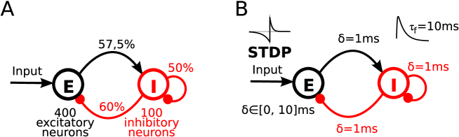
[Jonke et al., 2017] proposed a specific model for interacting populations of pyramidal cells with inhibitory neurons in cortical layer 2/3 based on data from the Petersen Lab [Avermann et al., 2012], see Fig. 1A, B. We refer to this specific model as the microcircuit motif model .
The model consists of two reciprocally connected pools of neurons, an excitatory pool and an inhibitory pool. stochastic spiking neurons constitute the excitatory pool. Their dynamics is given by a stochastic version of the spike response model that has been fitted to experimental data in [Jolivet et al., 2006]. The instantaneous firing rate of a neuron depends exponentially on its current membrane potential ,
| (1) |
where ms and are scaling parameters that control the shape of the response function. After emitting a spike, the neuron enters a refractory period.
The excitatory neurons are reciprocally connected to a pool of recurrently connected inhibitory neurons. All connection probabilities in the model were taken from [Avermann et al., 2012]. Excitatory neurons receive excitatory synaptic inputs with corresponding synaptic efficiencies between the input neuron and neuron . These afferent connections are subject to a standard form of STDP. Thus, the membrane potential of excitatory neuron is given by the sum of external inputs, inhibition from inhibitory neurons, and its excitability
| (2) |
where denotes the set of indices of inhibitory neurons that project to neuron , and denotes the weight of these inhibitory synapses. and denote synaptic input from inhibitory neurons and input neurons respectively, see above.
Inhibitory contributions to the membrane potential of pyramidal cells have in this neuron model a divisive effect on the firing rate. This can be seen by by substituting eq. (2) in eq. (1), see also eq. (23) in Methods, thus implementing divisive inhibition (see [Carandini and Heeger, 2012] for a recent review). Divisive inhibition has been shown to be a ubiquitous computational primitive in many brain circuits (see [Carandini and Heeger, 2012] for a recent review). In mouse visual cortex, divisive inhibition is implemented through inhibitory neurons [Wilson et al., 2012]. Although the inhibitory signal is common to all neurons in the pool of excitatory neurons, contrary to the inhibition modeled in [Nessler et al., 2013] it does not normalize the firing rates of neurons exactly and therefore the total firing rate in the excitatory pool is variable and depends on the input strength. Importantly, in contrast to [Nessler et al., 2013] where inhibition strictly enforced that only a single neuron in the excitatory pool is active at any given time, the data-based model allows several neurons to be active concurrently.
2.2 Emergent properties of the data-based network model: From WTA to k-WTA
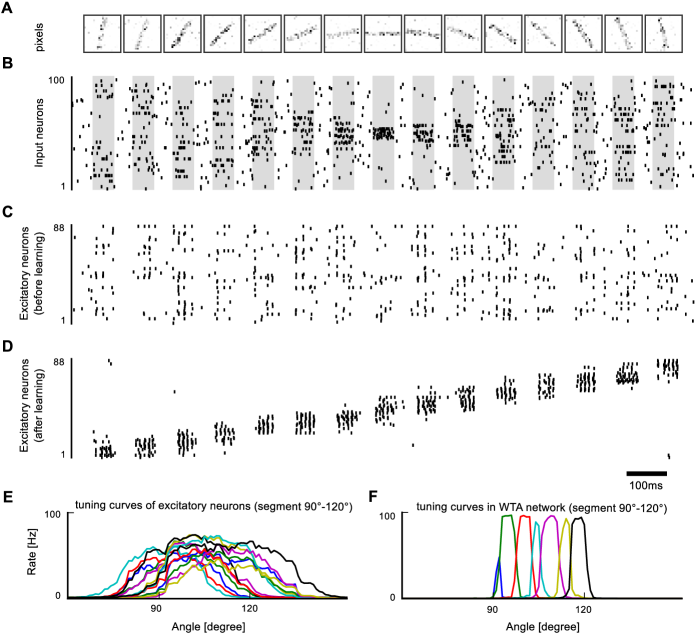
The computational properties of this data-based network model were extensively studied through simulations in [Jonke et al., 2017]. In order to compare the properties of this data-based network model to previously considered WTA models, they examined the emergence of orientation selectivity, which we briefly discuss here. For details, please see [Jonke et al., 2017]. Pixel-representations of noisy bars in random orientations were provided as external spike inputs (Fig. 2A). Input spike trains were generated from these pixel arrays by converting pixel values to Poisson firing rates of input neurons (black pixel: Hz; white pixel: Hz). Randomly oriented bars were presented to the network for s where each bar was presented for ms, see Fig. 2B (STDP was applied to synapses from input neurons to excitatory neurons). The resulting network response (Fig. 2D) shows the emergence of assembly codes for oriented bars. The resulting Gaussian-like tuning curves of excitatory neurons (Fig. 2E) densely cover all orientations, resembling experimental data from orientation pinwheels (see Fig. 2 d,e in [Ohki et al., 2006]). Also consistent with experimental data [Kerlin et al., 2010, Isaacson and Scanziani, 2011], inhibitory neurons did not exhibit orientation selectivity (not shown).
In contrast, previously considered models with idealized strong inhibition in WTA-circuits [Nessler et al., 2013] show a clearly distinct behavior, see Fig. 2F. For this model, at most a single neuron could fire at any moment of time, and as a result at most two neurons responded after a corresponding learning protocol with an increased firing rate to a given orientation (see Fig. 2F and Fig. 5 in [Nessler et al., 2013]). In the simulations of the data-based model , on average neurons responded to each orientation with an increased firing rate. This suggests that the emergent computational operation of the layer 2/3 microcircuit motif with divisive inhibition is better described as k-WTA computation, where winners may emerge simultaneously from the competition. This number is however not a strict constraint in the data-based model . The actual number of winners depends on synaptic weights and the external input. Its computation is thus better describe as an adaptive k-WTA operation. The k-WTA characterisitcs of the layer 2/3 microcircuit motif is quite attractive, since it is known from computational complexity theory that the k-WTA computation is more powerful than the simple WTA computation (for ) [Maass, 2000].
2.3 Theoretical framework for understanding emergent computational properties the layer 2/3 microcircuit motif
Fig. 2 demonstrates that significantly different computational properties emerge in the data-based model through STDP as compared to previously considered WTA models [Nessler et al., 2013, Habenschuss et al., 2013b]. The main aim of this article is to understand this different emergent computational capability theoretically, in particular since the analysis from [Nessler et al., 2013] and [Habenschuss et al., 2013b] in terms of mixture distributions is only applicable to WTA circuits. The novel analysis technique that we will use is summarized as follows. First, using some simplifications on the network dynamics, we formulate the network dynamics in the neural sampling framework [Buesing et al., 2011]. This allows us to deduce the distribution of activities of excitatory neurons in the network for a given input and for the given network weights . We then show that this distribution approximates the posterior distribution of a generative probabilistic model . This generative model is not a mixture distribution as in the WTA case [Nessler et al., 2013], but a more complex distribution that is based on a noisy-OR-like likelihood. We make the nature of the approximation explicit and evaluate its severity through simulations. Finally, we derive a plasticity rule that implement online EM in this generative model, thus implementing blind source separation. We find that this plasticity rule can be approximated by an STDP-like learning rule.
2.3.1 Formulation of the network dynamics of in the neural sampling framework
The neural sampling framework [Buesing et al., 2011] provides us with the ability to determine the stationary distribution (defined in the following) of network states for the given network parameters and a given network input. In order to be able to describe the probabilistic relationships between input and network activity, we describe network inputs by binary vectors and responses of excitatory neurons in by binary vectors . The vectors and capture the spiking activity of ensembles of spiking neurons in continuous time according to the common convention introduced in [Berkes et al., 2011] and [Buesing et al., 2011]: A spike of the neuron in the ensemble at time sets the corresponding component () of the bit vector () from its default value to for some duration (that can be chosen for example to reflect the typical time constant of an EPSP), see Methods. Note the difference between the vectors , and the output traces , used in eq. (2) (and defined in eq. (22) in Methods). The former constitute an abstract convention to describe the momentary state of the network based on its current firing activity, while the latter describe the impact that the neurons have on their postsynaptic targets in terms of real-valued double-exponential EPSPs.
We want to describe the distribution of network states for given inputs and network parameters in terms of a probability distribution . In this distribution, the activities of network inputs and excitatory neurons in are represented by two vectors of binary random variables: (termed input variables in the following) and (termed hidden variables or hidden causes). The network state at time is interpreted as one specific realization of these random variables.
In order to make this mapping between network activity in and the distribution of network states feasible, one has to make three simplifying assumptions about the dynamics of the neural network models similar as in [Buesing et al., 2011]. First, PSPs of inputs and network neurons are rectangular with length (chosen here to be ms) and network neurons are refractory for the same time span after each spike. Second, synaptic connections are idealized in the sense that the synaptic delay is (i.e., a presynaptic spike leads instantaneously to a PSP in the postsynaptic neuron). And finally, the weights of recurrent synaptic connections are symmetric (i.e., the weight from neuron to neuron is identical to the weight from neuron to neuron ). This necessitates that lateral inhibition is not implemented through a pool of inhibitory neurons. Instead, the network dynamics is defined by only one pool of network neurons (the same number as the number of excitatory network neurons in ). Since the inhibitory neurons in show linear response properties, the inhibition in the network depends linearly on the activity of excitatory neurons in the network. One can therefore model the inhibition in the network by direct inhibitory connections between excitatory neurons (where synaptic delays are neglected) with weight . For clarity, we provide the full description of the approximate dynamics in the following.
The approximate dynamics is described by network neurons. Network neurons have instantaneous firing rates that depend exponentially on their membrane potential, as given in eq. (1). Whenever neuron spikes, the output trace of neuron is set to for a period of duration (this corresponds to a rectangular PSP; the same definition applies to output traces of input neurons). After emitting a spike, the neuron enters a refractory period of duration ms, during which its instantaneous spiking probability is zero. Note that for this definition of the output trace, the state vector is identical to the vector of output traces . Lateral inhibition in the network is established by direct inhibitory connections between excitatory neurons, leading to membrane potentials
| (3) |
where denotes some neuron-specific excitability of the neuron that is independent of the input and network activity. Each network neuron receives feedforward synaptic inputs whose contribution to the membrane potential of a neuron at time depends on the synaptic efficiency between the input neuron and the network neuron . Network neurons are all-to-all recurrently connected. The second term in (3) specifies this recurrent input where is the inhibitory recurrent weight of the connection between network neuron and network neuron . It has been shown in [Buesing et al., 2011] that for such membrane potentials, the distribution of network states is given by the Boltzmann distribution:
| (4) |
where is a normalizing constant.
2.3.2 A probabilistic model for the layer 2/3 microcircuit motif:
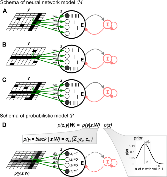
Fig. 3A-C illustrates the putative stochastic computation performed by the model , i.e., how network input leads to network activity in the model. Assume that we have a probabilistic model for the inputs defined by a prior and a likelihood . These distributions describe how one can generate input samples by first drawing a hidden state vector from and then drawing an input vector from . Therefore, such a probabilistic model is also called a generative model (for the inputs).
If the distribution of network states (4) is the posterior distribution given by
| (5) |
then the network performs probabilistic inference in this probabilistic model . The inference task described by eq. (5) assumes that is given and the hidden causes (such as the basic components of a visual scene) have to be inferred. This inference can intuitively also be described as providing an ”explanation” for the current observation according to the generative model . In the following, we describe a probabilistic model and show that eq. (4) approximates the posterior distribution of this model. This implies that the simplified dynamics of the data-based model approximate probabilistic inference in the probabilistic model .
The probabilistic model is defined by two distributions, the prior over hidden variables (that captures constraints on network activity imposed for example by lateral inhibition) and the conditional likelihood distribution over input variables that describes the probability of input for a given network state in a network with parameters . These two distributions define the joint distribution over hidden and visible variables since , see Fig. 3D. The specific forms of these two distributions in the probabilistic model considered for are discussed in the following and defined by eqs. (6)-(8) below.
In previously considered hard WTA models [Nessler et al., 2013, Habenschuss et al., 2013b], strong lateral inhibition was assumed. This corresponded to a prior where only a single component of the hidden vector can be active at any time. The biologically more realistic divisive inhibition in allows several of them to fire simultaneously. This corresponds to a prior that induces sparse activity in a soft manner (“adaptive” k-WTA): It does not enforce a strict ceiling on the number of -neurons that can fire within a time interval of length , but only tries to keep this number within a desired range. Hence we use as prior in a Gaussian distribution
| (6) |
where is a normalizing constant, is a parameter that shifts the mean of the distribution, and defines the variance (see Fig. 3D). Note that the Gaussian is restricted to integers as the sum runs over binary random variables .
As in other generative models we assume for the sake of theoretical tractability that the conditional likelihood factorizes, so that each input is independently explained by the current network state :
| (7) |
A probabilistic model for hard WTA circuits can only explain each input variable by a single hidden cause . In contrast, in probabilistic models with soft inhibition and the prior (6), several hidden causes can be active simultaneously and explain together an input variable . We define as the vector of weights that define the likelihood for variable . We consider the following likelihood model
| (8) |
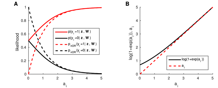
where we have defined , and is the logistic sigmoid . This likelihood function is shown in Figure 4A together with the often used noisy-OR likelihood. Note that if none of the hidden causes is active, i.e., for all , then with probability . Each active hidden cause with increases the probability that input variable assumes the value , see also Fig. 3D). This likelihood, allows the generative model to deal with situations where an input neuron can fire in the context of different hidden causes, for example with pixels in the network inputs that lie in the intersection of different patterns, see Fig. 3). The soft Gaussian prior (6) allows the internal model to develop modular representations for different components of complex input patterns. This likelihood is quite similar to the frequently used noisy-OR model (see e.g. [Neal, 1992, Saund, 1995]):
| (9) |
One difference is that (for purely excitatory weights), the probability of an input being zero is at most in the proposed likelihood, while it can become in the noisy-OR model. Such a model may reflect the situation that network inputs are noisy, so their firing rates are never zero.
We now analyze the relationship between the probabilistic model and the description of the data-based model in the neural sampling framework. We will see that approximates probabilistic inference in . Finally, we show that adaptation of network parameters in through STDP can be understood as an approximate stochastic expectation maximization (EM) process in the corresponding probabilistic model .
2.3.3 Interpretation of the dynamics of in the light of :
Using the likelihood and prior of , the posterior of hidden states for given inputs and given parameters is
| (10) |
where is a normalizing constant, , and . The terms including and stem from the prior, while the last term stems from the normalization of the likelihood. When we compare this posterior to the posterior of the network model eq. (4), we see that they are quite similar with denoting the strength of inhibitory connections and being the neural excitabilities.
The last term in eq. (10) is problematic since the ’s depend on and thus the whole posterior is not a Boltzmann distribution and can therefore not be computed by the model . It turns out however that this last term can be approximated quite well by a term that is linear in . Note that for zero (i.e., for zero weights or for the zero--vector), this last term evaluates to . But as increases, one can neglect the in the logarithm and the expression quickly approaches . We can thus write
| (11) |
where the term in the brackets on the right is just the L1-norm of the weight vector of neuron . Note that for a given weight matrix, an increased leads to a better approximation. The approximation of by is illustrated in Fig. 4B. Hence, the first approximate posterior we consider is given by
| (12) |
This is a Boltzmann distribution of the form (4) and the last term accounts to a neuron-specific homeostatic bias that depends on the sum of incoming excitatory weights. Matching the terms of this equation to the terms in eq. (4) and performing the same match in the membrane potential (3), we see that the membrane potential of neurons in this approximation is given by
| (13) |
If excitatory weight vectors are normalized to an L1-norm of for all , this simplifies to
| (14) |
Note that can be incorporated into . Such constant weight sum could be enforced in a biological network by a synaptic scaling mechanism [Turrigiano and Nelson, 2004, Savin et al., 2010] that normalizes the sum of incoming weights to a neuron. For the data-based model , [Jonke et al., 2017] used uniform excitabilities for all excitatory neurons and no homeostasis for simplicity, see eq. (2). We will argue below under which conditions this approximation is justified. We consider the posterior distribution of such circuits as our second approximation of the exact posterior:
| (15) |
Note that in this case, effectively leads to a smaller mean of the Gaussian prior. A detailed discussion about how parameters of the generative probabilistic model can be mapped to parameters of the data-based microcircuit motif model is provided in Network parameter interpretation in Methods.
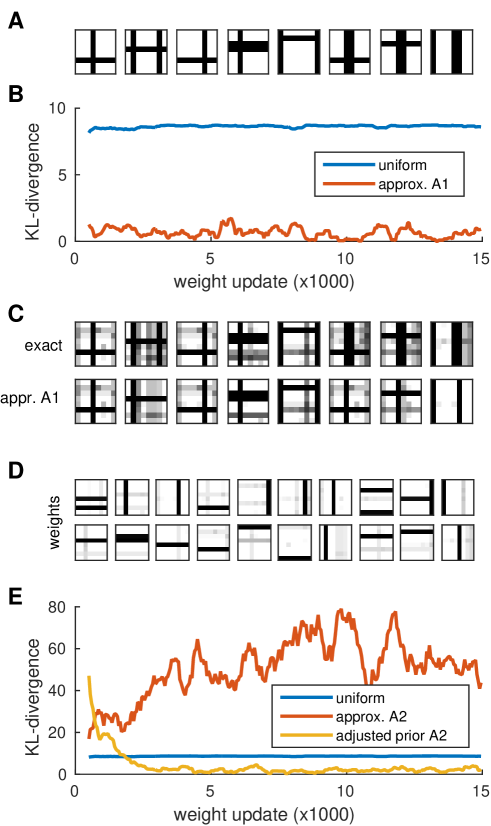
We evaluated the impact of these two approximations in Földiak’s superposition-of-bars problem [Földiak, 1990]. This is a standard blind-source separation problem that has also been used in [Jonke et al., 2017] to evaluate the data-based network model . In this problem, input patterns are two-dimensional pixel arrays on which horizontal and vertical bars (lines) are superimposed, see Fig. 5A. Input patterns were generated with a superposition of 1 to 3 bars from the distribution that was used in [Jonke et al., 2017]. We performed inference of hidden causes by sampling from the approximate posterior distribution given by eq. (12) for a network of 20 hidden-cause neurons. We performed approximate stochastic online EM in order to optimize the parameters of the model. The synaptic update rule (20) used for parameter updates is discussed in detail below. We compared the approximated posterior to the exact one (10) by computing the Kullback-Leibler (KL) divergence . The KL divergence was small throughout learning, with a slight decrease during the process, see Fig. 5B (mean KL divergence during the second half of training was ). To evaluate what that KL-divergence means for the inference, we considered the hidden state vector with the maximum posterior probability after learning in the exact and approximate posterior and used this to reconstruct the input pattern by computing . The reconstructed inputs for the 8 example inputs of Fig. 5A are shown in Fig. 5C for the exact posterior (top) and the approximate posterior (bottom). The approximate reconstructions resemble the exact ones in many cases, with occasional misses of a basic pattern. The final weights of the 20 neurons are shown in Fig. 5D in the two-dimensional layout of the input to facilitate interpretability. Note that all basic patterns were represented by individual neurons with additional neurons that specialized on combined patterns.
The approximate posterior is equivalent to the approximate posterior if the synaptic weights of each neuron are normalized to a common norm. It turned out in [Jonke et al., 2017] that such a normalization is not strictly necessary. In this work, the data-based model managed to perform blind source separation with a posterior that can be best described by without normalization of synaptic efficacies. We found that for the superposition-of-bars problem, the posterior distribution differs significantly from the exact posterior if we set in eq. (15), see red line in Fig. 5E. This difference is mostly induced by the tendency of to prefer many hidden causes due to the missing last term in eq. (15). If the prior was corrected to reduce the number of hidden causes, we found that the approximation was significantly improved, in particular as the network weight vectors approached their final norm values, see yellow line in Fig. 5E. A closer inspection of eq. (15) in comparison with eq. (12) shows that this approximation is effective if basic patterns consist of a similar number of active units, because otherwise patterns with strong activity are preferred over weakly active ones (this is exactly what the last term in eq. (12) compensates for).
We conclude from this analysis that the microcircuit motif model approximates probabilistic inference in a noisy-OR-like probabilistic model of its inputs. The prior on network activity favors sparse network activity, but does not strictly enforce a predefined activity level. Such a more flexible regulation of network activity is obviously important when the network input is composed of a varying number of basic component patterns. We show below that this network behavior in combination with STDP allows the microcircuit motif model to perform blind source separation of mixed input sources. Our analysis above has shown that the computation of blind source separation in can be facilitated either by the normalization of activity in input populations, or by homeostatic mechanisms that normalize excitatory synaptic efficacies within each neuron.
2.3.4 STDP in the microcircuit motif model creates an internal model of network inputs:
After we have established a link between a well-defined probabilistic model and the spiking dynamics of microcircuit motif model , we can now analyze plasticity in the network. The probabilistic model defines a likelihood distribution over inputs that depends on the parameters through
| (16) |
where the sum runs over all possible hidden states .
We propose that STDP in can be viewed as an adaptation of the parameters so that as defined by the probabilistic model with parameters approximates the actually encountered distribution of spike inputs within the constraints of the prior . Since the prior typically is defined to favor sparse representations, this tends to extract the hidden sources of these patterns, an operation called blind source separation [Földiak, 1990].
More precisely, we show that STDP in approximates stochastic online EM [Sato, 1999, Bishop, 2006] in . Given some external distribution of synaptic inputs, EM adapts the model parameters such that the model likelihood distribution approximates the given distribution . More formally, the Kullback-Leibler divergence between the likelihood of inputs in the internal model and the empirical data distribution is brought to a local minimum. The theoretically optimal learning rule for EM contains non-local terms which are hard to interpret from a biological point of view. In the following, we derive a local approximation to yield a simple STDP-like learning rule.
The goal of the EM algorithm is to find parameters that (locally) minimize the Kullback-Leibler divergence between the likelihood of inputs in the probabilistic model and the empirical data distribution , that is, the distribution of inputs experienced by the network . This is equivalent to the maximization of the average data log-likelihood . For a given set of training data and corresponding unobserved hidden variables , this corresponds to maximizing . The optimization is done by iteratively performing two steps. For given parameters , the posterior distribution over hidden variables is determined (the E-step). Using this distribution, one then performs the M-step where is maximized with respect to to obtain better parameters for the model. These steps are guaranteed to increase (if not already at a local optimum) a lower bound on the data log likelihood, that is, . These steps are iterated until convergence of parameters to a local optimum [Bishop, 2006]. Computation of the M-step in the probabilistic model is hard. In the generalized EM algorithm, the M-step is replaced by a procedure that just improves the parameters, without necessarily obtaining the optimal ones for a single M-step. This can be done for example by changing the parameters in the direction of the gradient
| (17) |
Since in our model, we assume that synaptic efficacy changes are instantaneous for each pre-post spike pair, we need to consider an online-version of the generalized EM algorithm. In stochastic online EM, for each data example , a sample from the posterior is drawn (the stochastic E-step) and parameters are changed according to this sample-pair. As shown above, the network implements an approximation of the stochastic E-step. In the M-step, each parameter is then updated in the direction of the gradient . As the prior in does not depend on , this is equivalent to . For the likelihood given by eq. (8), this derivative is given by
| (18) |
where denotes the logistic sigmoid function. Hence, the synaptic update rule for weight is given by
| (19) |
where is a learning rate. This learning rule is not local as it requires information about the activation of all output neurons as well as values of all synaptic weights originating from input neuron . In order to make this biologically plausible we approximate rule (19) by
| (20) |
This rule uses only locally available information at the synapse. What are the consequences of this approximation during learning? If only a single neuron in the network is active, then the approximation is exact. Otherwise, the approximation ignores what other neurons contribute to the explanation of input component . This means that for , the weight will further be increased even if is already fully explained by the network activity. For , the decrease will in general be smaller than in the exact rule (since weights are non-negative). Note however that only the magnitudes of weigh changes are affected, but not which weights change and the sign of the change. Hence, we can conclude that the angle between the approximate parameter change vector and the exact parameter change vector is between and degrees. In other words, the inner product of these two vectors is always non-negative and the updates are performed in the correct direction. This was confirmed in simulations. In the learning experiment described in Fig. 5, we compared the approximate update (that was used to optimize the model) with the update that was proposed by the exact rule (18) at every update step. The angle between the exact and approximate update vector was between and with a mean of .
In the simplified dynamics, a value of is indicated by a spike in network neuron when pattern is presented as input. We therefore map this update to the following synaptic plasticity rule: For each postsynaptic spike, update weight according to
| (21) |
According to this learning rule, when the presynaptic neuron spikes shortly before the postsynaptic neuron this results in long-term potentiation (LTP) which is weight dependent according to the term . Due to the weight dependence, large weights lead to small weight changes, with vanishing changes for very large weights. When a post-synaptic spike by neuron is not preceded by a presynaptic spike by neuron (e.g. when the pre-synaptic spike comes after the post-synaptic spike), this results in long term depression (LTD). LTD is also weight dependent, but to a much lesser extent as the weight-dependent factor varies only between and . This behavior is mimicked by the standard STDP rule implemented in the data-based model that a standard weight dependence where updates exponentially decreased with for LTP and did not depend on for LTD.
Hence, the dynamics and synaptic plasticity of the data-based model can be understood as an approximation of EM in the probabilistic model , that creates an internal model for the distribution of network inputs. This internal probabilistic model is defined by a noisy-OR-like likelihood term and a sparse prior on the hidden causes of the current input pattern. Hence, STDP can be understood as optimizing model parameters such that the observed distribution of input patterns can be explained through a set of basic patterns (hidden causes). It is assumed that the input at each time point can be described by a combination of a sparse subset of these patterns. In other words, STDP in the microcircuit motif model performs blind source separation of input patterns.
3 Discussion
We have provided a novel theoretical framework for analyzing and understanding computational properties that emerge from STDP in a prominent cortical microcircuit motif: interconnected populations of pyramidal cells and interneurons in layer 2/3. The computer simulations in [Jonke et al., 2017], that were based on the data from [Avermann et al., 2012], indicate that the computational operation of this network motif cannot be captured adequately by a WTA model. Instead, this work suggests a k-WTA model, where a varying number of the most excited neurons become active. Since the WTA circuit model turns out to be inadequate for capturing the dynamics of interacting pyramidal cells and interneurons, one needs to replace the probabilistic model that one had previously used to analyze the impact of STDP on the computational function of the network motif. Mixture models such as those proposed by [Nessler et al., 2013] and [Habenschuss et al., 2013b] are inseparably tied to WTA dynamics: For drawing a sample from a mixture model one first decides stochastically from which component of the mixture model this sample should be drawn (and only a single component can be selected for that). We have shown here that a quite different generative model, similar to the noisy-OR model, captures the impact of soft lateral inhibition on emergent network codes and computations much better (Fig. 3). The noisy-OR model is well-known in machine learning [Neal, 1993, Saund, 1995], but has apparently not previously been considered in computational neuroscience. Our probabilistic model further suggests that the varying number of active neurons in the circuit may depend both on a prior that is encoded by the network parameters and the familiarity of the network input.
We have shown that the evolution of the dynamics and computational function of the network motif under STDP can be understood from the theoretical perspective as an approximation of expectation maximization (EM) for fitting a noisy-OR based generative model to the statistics of the high dimensional spike input stream. This link to EM is very helpful from a theoretical perspective, since EM is one of the most useful theoretical principles that are known for understanding self-organization processes. In particular, this theoretical framework allows us to elucidate emergent computational properties of the network motif for spike input streams that contain superimposed firing patterns from upstream networks. It disentangles these patterns and represents the occurrence of each pattern component by a separate sparse assembly of neurons, as already postulated in [Földiak, 1990].
The established relationship between the network and the probabilistic model allows us to relate the network parameters and (eq. (2)) of to the parameters of the generative model . Briefly (for a detailed discussion, see Network parameter interpretation in Methods), the excitability of pyramidal cells is proportional to , see eq. (26). The strength of inhibitory connections to the pool of pyramidal cells is proportional to , see eq. (30). Hence, a large in combination with a small (i.e., a sharp activity prior), leads to a large spontaneous activity that is tightly regulated by strong inhibitory feedback. On the other hand, a broad prior (larger ) leads to weaker inhibitory feedback, thus allowing the network to attain a broader range of activities.
Related work
A related theoretical study for WTA circuits was performed in [Nessler et al., 2013, Habenschuss et al., 2013a, Kappel et al., 2014] and extended to sheets of WTA circuits in [Bill et al., 2015]. It was assumed in these models that inhibition normalizes network activity exactly, leading to a strict WTA behavior. The analysis in the present work is much more complex and necessarily has to include a number of approximations. Out analysis reveals that the softer type of inhibition that we studied provides the network with additional computational functionality. There exists also a structural similarity of the proposed learning rule (21) to those reported in [Nessler et al., 2013, Habenschuss et al., 2013a, Kappel et al., 2014]. This is insofar significant as it raises the question why the application of almost the same learning rule in one motif leads to learning and extraction of a single hidden cause and in another to the extraction of multiple causes. The answer most likely lies in the interplay between “prior knowledge” in the model (e.g. in the form of the intrinsic excitability of neurons), the learning rule and inhibition strength: As there are multiple neurons in the proposed microcircuit motif model which can spike in response to the same input, each one of them can adapt its synaptic weights to increase the likelihood of spiking again whenever the same or a similar input pattern is presented in the future, possibly in conjunction with other different input components. This is manifested through increased total input strength to those neurons when the pattern is seen again. But this results also in increased total inhibition to all other neurons, thereby effectively limiting the number of winners. As there is no fixed normalization of firing rates (probabilities), as soon as the input strength caused by a single feature component is strong enough to trigger the spike in some neuron, the neuron will respond to each pattern which consists of that particular feature. On average this will force neurons to specialize on a single feature component. Therefore, after learning, each spike can be interpreted as indication of a particular feature component.
The noisy-OR model eq. (9) is tightly related to the likelihood model used in this article. It is one of the most basic likelihood models that allows to combine basic patterns. Noisy-OR and related models have previously been used in the machine learning literature as models for nonlinear component extraction [Saund, 1995, Lücke and Sahani, 2008], or as basic elements in belief networks [Neal, 1992], but they have so far not been linked to cortical processing.
The extraction of reoccurring components of input patterns is closely related to blind source separation and independent component analysis (ICA) [Hyvärinen et al., 2004]. Previous work in this direction includes implementations of ICA in artificial neural networks [Hyvärinen, 1999], see also [Lücke and Eggert, 2010]. These abstract models are only loosely connected to computation in cortical network motifs. [Savin et al., 2010] investigated ICA in the context of spiking neurons. Theoretical rules for intrinsic plasticity were derived which enable neurons in combination with input normalization, weight scaling, and STDP, to extract independent components of inputs. An interesting difference is that the inhibition in [Savin et al., 2010] acts to decorrelate neuronal activity. Intrinsic plasticity on the other hand enforces sparse activity (this sparsening has to happen on the time scale of input presentations). In our probabilistic model , sparse network activity is enforced by a prior over network activities, implemented in through the inhibitory feedback that models experimentally found network connectivity [Avermann et al., 2012]. This inhibition naturally acts on a fast time scale [Okun and Lampl, 2008], while the time scale for intrinsic plasticity is unclear [Turrigiano and Nelson, 2004].
4 Methods
4.1 Definition of : Data-based network model for a layer 2/3 microcircuit motif
The layer 2/3 microcircuit motif was modeled in [Jonke et al., 2017] by the data-based model . The model is described here briefly for completeness. See [Jonke et al., 2017] for a thorough definition. The model consists of two reciprocally connected pools of neurons, an excitatory pool and an inhibitory pool. Inhibitory network neurons are recurrently connected. Excitatory network neurons receive additional excitatory synaptic input from a pool of input neurons. Fig. 1A summarizes the connectivity structure of the data-based model together with connection probabilities. Connection probabilities have been chosen according to the experimental data described in [Avermann et al., 2012].
Let denote the spike times of input neuron . The output trace of input neuron is given by the temporal sum of unweighted postsynaptic potentials (PSPs) arising from input neuron :
| (22) |
where is the synaptic response kernel, i.e., the shape of the PSP. It is given by a double-exponential function with a rise time constant ms and a fall time constant ms. For given spike times, output traces of excitatory network neurons and inhibitory network neurons are defined analogously and denoted by and respectively.
The network consists of excitatory neurons, modeled as stochastic spike response model neurons [Jolivet et al., 2006], see eqs. (1) and (2). See Sec. 4.2 for a motivation of network parameter values from a theoretical perspective.
The instantaneous firing rate of neuron can be re-written (by substituting eq. (2) in eq. (1)) as:
| (23) |
Here, the numerator includes all excitatory contributions to the firing rate . The denominator in this term for the firing rate describes inhibitory contributions, thereby reflecting divisive inhibition [Carandini and Heeger, 2012].
Apart from excitatory neurons there are inhibitory neurons in the network. Inhibitory neurons are also modeled as stochastic spike response neurons with an instantaneous firing rate given by
| (24) |
where denotes the linear rectifying function for and otherwise. The membrane potentials of inhibitory neurons are given by
| (25) |
where denotes synaptic input (output trace) from excitatory network neuron , () denotes the set of indices of excitatory (inhibitory) neurons that project to inhibitory neuron , and () denotes the excitatory (inhibitory) weight to inhibitory neurons.
Synaptic connections from input neurons to excitatory network neurons are subject to STDP. A standard version of STDP is employed with an exponential weight dependency for potentiation [Habenschuss et al., 2013b], see [Jonke et al., 2017].
The simulations for Fig. 2 are described in detail in [Jonke et al., 2017].
4.2 Network parameter interpretation:
In the section Interpretation of the dynamics of in the light of , we have established a relationship between the parameters of the probabilistic model and network parameters. This relationship was however derived based on a simplified network model that included for example rectangular EPSPs and direct inhibitory connections without explicit inhibitory neurons. Nevertheless, one can also determine reasonable parameter settings for the data-based model based on a prior on network activity that is defined in the probabilistic model . These parameters are the excitability and the synaptic weights between and within excitatory and inhibitory network neurons.
In this section we start by assuming such a prior eq. (6) with parameters (this includes already a correction of the prior for the missing ) and as well as a fitting parameter (eq. 1) and deduce the parameters used in the simulations. As shown above, the neural excitability is then given by . We obtain for the chosen :
| (26) |
The inhibition strength of the approximate dynamics eq. (3) is replaced by the weight from inhibitory neurons to excitatory neurons in . From the probabilistic model, we determined as under the assumption of rectangular inhibitory PSPs. In we use double-exponential PSPs instead of rectangular ones. One therefore has to correct for differences in the PSP integrals. Using this correction, one obtains
| (27) |
where is the ratio between the integrals over the rectangular PSPs used in the approximate dynamics and the double-exponential PSPs used in ( for the shapes used for ).
The weights can be determined by comparing eq. (2) with eq. (3) with corrected inhibition strength
| (28) |
Under the assumption that the number of spikes in the pool of inhibitory neurons is at any time (with a slight delay) approximately equal to the number of spikes in the pool of excitatory neurons, we obtain
| (29) |
where denotes the connection probability from inhibitory to excitatory network neurons. This yields
| (30) |
We now first consider the weights from excitatory to inhibitory neurons under the assumption of no I-to-I connections. In this case, in order to obtain the same number of spikes in the inhibitory neurons as in the excitatory neurons, each spike from an excitatory neuron should induce on average one spike within all inhibitory neurons, that is,
| (31) |
where is the integral over the alpha-PSPs, is the connection probability from excitatory to inhibitory neurons, and is the number of inhibitory neurons. We obtain
| (32) |
Without I-to-I connections, this guarantees that excitation is balanced by inhibition. However, the single spike (on average) will occur on average with a delay of ms. Interestingly, the I-to-I connections can help to decrease this delay. In particular, if one demands that the inhibitory spike is elicited with a delay of less than one ms on average, then one can simply increase the weights by some factor , leading to
| (33) |
Now, each spike in the excitatory population induces in the inhibitory population for approximately ms a total rate of Hz, leading to an average delay of ms. Without I-to-I connections this would however lead to too many successive spikes within these ms. The I-to-I connections can compensate this too large excitation. For an approximately correct compensation, the first inhibitory spike has to balance out this excitation, which is approximately achieved by providing exactly the same amount of inhibition to inhibitory neurons, leading to
| (34) |
Since , we used for simplicity. These are the parameter values used for the model in [Jonke et al., 2017].
4.3 Details to simulations for Figure 5
Creation of basic patterns: Basic patterns were -dimensional vectors, each representing a horizontal or vertical bar on an two-dimensional pixel array. We defined basic patterns in total, corresponding to all possible horizontal and vertical bars of width in this pixel array. For a horizontal (vertical) bar, all pixels of a row (column) in the array attained the value while all other pixels were set to . The entries of the basic pattern vectors were then defined by the values of the corresponding pixels in the array.
Superposition of basic patterns: To generate an input pattern, basic rate patterns were superimposed as follows. The number of superimposed basic patters was chosen between and drawn from the distribution . Then each basic pattern to be superimposed was drawn uniformly from the set of basic patterns without replacement. This corresponds to the distribution used in [Jonke et al., 2017]. The input vector was then given by , where denotes the basic pattern to be superimposed and the operation is performed element-wise.
Optimization of the generative model: The generative model (6)–(8) with hidden causes was fitted to this data in an iterative manner. One iteration of the fitting algorithm was performed as follows:
-
1.
draw an input vector as described above;
-
2.
draw a sample from the approximate posterior , eq. (12);
-
3.
update the parameters of the model according to eq. (20).
Since the posterior in step (2) is intractable, it was approximated by assuming that a maximum of hidden causes are active in the posterior distribution (state vectors with more active hidden causes usually had negligible probabilities). This allowed us to compute the partition function and therefore to sample hidden state vectors in a straight-forward manner. Further, we did not consider hidden state vectors with no active hidden state since those would not lead to any parameter changes.
Parameters of the model and learning rule: A prior distribution with parameters and was used. The scaling parameter was set to . Weights were initialized with values drawn from a uniform distribution in . Weights were clipped between a minimal value of and a maximal value of . A constant learning rate of was used. Training was performed for updates. Network characteristics (such as KL divergences) were computed every update.
Figure 5B: Every update, we computed the KL-divergence between the true posterior and the approximate posterior . In addition we also computed the KL-divergence between and a uniform distribution over state vectors. In all these divergences, we only considered the distribution over vectors with at most active hidden causes for tractability (see above). For Fig. 5B, the data was smoothed using a box-car filter of size .
Figure 5C: We considered the input patters given in panel A and computed the hidden state with the maximum posterior probability (computed as described above) after learning in the exact and approximate posterior. This hidden state vector was then used to reconstruct the input pattern by computing . Note that this is not a sample of but it defines the probability of each individual pixel to be .
Figure 5E: Every update of the simulation described above, we computed the KL-divergence between the true posterior and the posterior according to approximation . For the red curve we used with and the same as given for the original model. For the yellow curve, we corrected the prior of the model to have . The KL-divergence to the uniform distribution was computed as described above.
Acknowledgements: Written under partial support by the Human Brain Project of the European Union #604102 and #720270, and the Austrian Science Fund (FWF): I 3251-N33.
References
- [Avermann et al., 2012] Avermann, M., Tomm, C., Mateo, C., Gerstner, W., and Petersen, C. (2012). Microcircuits of excitatory and inhibitory neurons in layer 2/3 of mouse barrel cortex. Journal of neurophysiology, 107(11):3116–3134.
- [Berkes et al., 2011] Berkes, P., Orban, G., Lengyel, M., and Fiser, J. (2011). Spontaneous cortical activity reveals hallmarks of an optimal internal model of the environment. Science, 331:83–87.
- [Bill et al., 2015] Bill, J., Buesing, L., Habenschuss, S., Nessler, B., Maass, W., and Legenstein, R. (2015). Distributed bayesian computation and self-organized learning in sheets of spiking neurons with local lateral inhibition. PloS one, 10(8):e0134356.
- [Bishop, 2006] Bishop, C. M. (2006). Pattern Recognition and Machine Learning. Springer, New York.
- [Buesing et al., 2011] Buesing, L., Bill, J., B., and Maass, W. (2011). Neural dynamics as sampling: A model for stochastic computation in recurrent networks of spiking neurons. PLoS Computational Biology, 7(11):e1002211.
- [Carandini and Heeger, 2012] Carandini, M. and Heeger, D. J. (2012). Normalization as a canonical neural computation. Nature Reviews Neuroscience, 13(1):51–62.
- [Douglas and Martin, 2004] Douglas, R. J. and Martin, K. A. (2004). Neuronal circuits of the neocortex. Annual Reviews of Neuroscience, 27:419–451.
- [Fino et al., 2012] Fino, E., Packer, A. M., and Yuste, R. (2012). The logic of inhibitory connectivity in the neocortex. The Neuroscientist, 19(3):228–237.
- [Földiak, 1990] Földiak, P. (1990). Forming sparse representations by local anti-hebbian learning. Biological cybernetics, 64(2):165–170.
- [Habenschuss et al., 2013a] Habenschuss, S., Jonke, Z., and Maass, W. (2013a). Stochastic computations in cortical microcircuit models. PLoS Computational Biology, 9(11):e1003311.
- [Habenschuss et al., 2013b] Habenschuss, S., Puhr, H., and Maass, W. (2013b). Emergence of optimal decoding of population codes through STDP. Neural computation, 25(6):1371–1407.
- [Hyvärinen, 1999] Hyvärinen, A. (1999). Fast and robust fixed-point algorithms for independent component analysis. Neural Networks, IEEE Transactions on, 10(3):626–634.
- [Hyvärinen et al., 2004] Hyvärinen, A., Karhunen, J., and Oja, E. (2004). Independent Component Analysis. John Wiley & Sons.
- [Isaacson and Scanziani, 2011] Isaacson, J. S. and Scanziani, M. (2011). How inhibition shapes cortical activity. Neuron, 72(2):231–243.
- [Jolivet et al., 2006] Jolivet, R., Rauch, A., Lüscher, H., and Gerstner, W. (2006). Predicting spike timing of neocortical pyramidal neurons by simple threshold models. Journal of Computational Neuroscience, 21:35–49.
- [Jonke et al., 2017] Jonke, Z., Legenstein, R., Habenschuss, S., and Maass, W. (2017). Feedback inhibition shapes emergent computational properties of cortical microcircuit motifs. arXiv preprint arXiv:1705.07614.
- [Kappel et al., 2014] Kappel, D., Nessler, B., and Maass, W. (2014). STDP installs in winner-take-all circuits an online approximation to hidden markov model learning. PLoS Comput. Biol, 10:e1003511.
- [Kerlin et al., 2010] Kerlin, A. M., Andermann, M. L., Berezovskii, V. K., and Reid, R. C. (2010). Broadly tuned response properties of diverse inhibitory neuron subtypes in mouse visual cortex. Neuron, 67(5):858–871.
- [Klampfl and Maass, 2013] Klampfl, S. and Maass, W. (2013). Emergence of dynamic memory traces in cortical microcircuit models through stdp. The Journal of Neuroscience, 33(28):11515–29.
- [Lücke and Eggert, 2010] Lücke, J. and Eggert, J. (2010). Expectation truncation and the benefits of preselection in training generative models. The Journal of Machine Learning Research, 9999:2855–2900.
- [Lücke and Sahani, 2008] Lücke, J. and Sahani, M. (2008). Maximal causes for non-linear component extraction. The Journal of Machine Learning Research, 9:1227–1267.
- [Maass, 2000] Maass, W. (2000). On the computational power of winner-take-all. Neural Computation, 12(11):2519–2535.
- [Neal, 1992] Neal, R. M. (1992). Connectionist learning of belief networks. Artificial intelligence, 56(1):71–113.
- [Neal, 1993] Neal, R. M. (1993). Probabilistic inference using markov chain monte carlo methods. Technical report, University of Toronto Department of Computer Science.
- [Nessler et al., 2013] Nessler, B., Pfeiffer, M., Buesing, L., and Maass, W. (2013). Bayesian computation emerges in generic cortical microcircuits through spike-timing-dependent plasticity. PLoS Computational Biology, 9(4):e1003037.
- [Ohki et al., 2006] Ohki, K., Chung, S., Kara, P., Hübener, M., Bonhoeffer, T., and Reid, R. C. (2006). Highly ordered arrangement of single neurons in orientation pinwheels. Nature, 442(7105):925–928.
- [Okun and Lampl, 2008] Okun, M. and Lampl, I. (2008). Instantaneous correlation of excitation and inhibition during ongoing and sensory-evoked activities. Nature Neuroscience, 11(5):535–537.
- [Packer and Yuste, 2011] Packer, A. M. and Yuste, R. (2011). Dense, unspecific connectivity of neocortical parvalbumin-positive interneurons: a canonical microcircuit for inhibition? The Journal of Neuroscience, 31(37):13260–13271.
- [Rumelhart and Zipser, 1985] Rumelhart, D. E. and Zipser, D. (1985). Feature Discovery by Competitive Learning. Cognitive Science, 9(1):75–112.
- [Sato, 1999] Sato, M. (1999). Fast learning of on-line EM algorithm. Technical report, ATR Human Information Processing Research Laboratories, Kyoto, Japan.
- [Saund, 1995] Saund, E. (1995). A multiple cause mixture model for unsupervised learning. Neural Computation, 7(1):51–71.
- [Savin et al., 2010] Savin, C., Joshi, P., and Triesch, J. (2010). Independent component analysis in spiking neurons. PLoS computational biology, 6(4):e1000757.
- [Turrigiano and Nelson, 2004] Turrigiano, G. G. and Nelson, S. B. (2004). Homeostatic plasticity in the developing nervous system. Nature Reviews Neuroscience, 5(2):97–107.
- [Wilson et al., 2012] Wilson, N. R., Runyan, C. A., Wang, F. L., and Sur, M. (2012). Division and subtraction by distinct cortical inhibitory networks in vivo. Nature, 488(7411):343–348.