On the analysis of signals in a permutation Lempel–Ziv complexity - permutation Shannon entropy plane

Abstract

The aim of this paper is to introduce the Lempel–Ziv permutation complexity vs permutation entropy plane as a tool to analyze time series of different nature. This two quantities make use of the Bandt and Pompe representation to quantify continuous-state time series. The strength of this plane is to combine two different perspectives to analyze a signal, one being statistic (the permutation entropy) and the other being deterministic (the Lempel–Ziv complexity). This representation is applied (i) to characterize non-linear chaotic maps, (ii) to distinguish deterministic from stochastic processes and (iii) to analyze and differentiate fractional Brownian motion from fractional Gaussian noise and $K$-noise given a same (averaged) spectrum. The results allow to conclude that this plane is “robust” to distinguish chaotic signals from random signals, as well as to discriminate between different Gaussian and nonGaussian noises.

1 Introduction

The signals coming from the real world often have very complex dynamics and/or come from coupled dynamics of many dimensional systems. We can find an endless number of examples arising from different fields. In physiology, one can mention the reaction-diffusion process in cardiac electrical propagation that provides electrocardiograms, or the dynamics underlying epileptic electroencephalograms (EEGs) [1, 2]. The world of finance or social systems are also good examples of how “complexity” emerges from these systems [3, 4, 5]. One important challenge is then to be able to extract relevant information from these complex series [6, 7, 8].

To address this issue, the researchers generally analyze these signals using tools that come either from probabilistic analysis, or from nonlinear dynamics. The idea in the first approach is to measure the spread of the statistical distribution underlying the data, to detect changes in this distribution, to analyze the spectral contents of the signals, etc. Among the panel of tools generally employed, that coming from the information theory take a particular place [9, 10, 11]. The second approach is well suited for signals having a deterministic origin, generally non linear. The tools usually employed come from the chaos world, such that the fractal dimensions, the Lyapunov exponents, among many others [6, 12], or from the concept of complexity in the sense of Kolmogorov (e.g.,the Lempel–Ziv complexity) [13, 14, 15]

It has been recently proposed to analyze time series by the use of a “complexity–entropy plane”, exhibiting that the joint use of two quantities gives a richer information about the series than each measure separately (see [16] for the introduction of signal analysis in an information plane). Such planes have been used in the literature in various areas, for instance to differentiate chaotic series from random signals [17], to characterize chaotic maps [18], to determine the authorship of literary texts [19], to quantify the stock market inefficiency [20], or for the analysis of the EEG dynamics [21]. In the mentioned works, the complexity used are based on statistical measures, for instance the “statistical complexity measure” making use of the entropy [22], however the information obtained from the time series is thus purely statistical. In this work, we propose to use both statistical and deterministic measures namely, the well known Shannon entropy and Lempel–Ziv complexity [23, 24]. Additionally, to calculate the Lempel–Ziv complexity as well as the Shannon entropy, it is necessary to deal with time series taking their values over a discrete finite size alphabet . Nevertheless, in the “real life” we generally face to continuous-state data. Thus, the quantization of the signal is a fundamental issue of the analysis.

Many methods to quantify continuous data exist in the literature, from nonparametric estimators making use of nearest neighbors or graph lengths for instance [25, 27, 26, 28, 29], to quantizers based on Parzen–Rosenblatt approaches (–for instance with square kernel, i.e..,using histograms) [30, 31]. In this paper, we focus on an approach proposed by Bandt and proposed a decade ago, based on a multivariate trajectory built from the scalar series, i.e..,an embedding, and the so-called permutation vectors constructed from this embedding [32]. More precisely, for each point of the embedded trajectory, the vectors components are sorted and the values are replaced by their rank. In their paper, they used these permutation vectors to propose what they called permutation entropy, that is nothing more than the empirical estimate of the Shannon entropy of the permutation vectors [32]. In the same vein, we proposed recently the use of the Lempel–Ziv complexity applied to permutation vectors for the analysis of continuous-states sequences, leading to what we named permutation Lempel–Ziv complexity [33]. The same approach is envisaged here, but instead of working with one of the two single measures, we propose to study various systems or sequences in an entropy-complexity plane trying to characterize various type of behaviors from different time series.

The paper is organized as follows. Section 2 gives a brief introduction on the measures used for the analysis. Section 3 describes the permutation method we use to quantize the series, i.e..,the procedure to obtain the permutation vectors. Then, section 4 presents characterizations of the chaotic maps and noises we analyze in the present work while their analysis in the complexity–entropy plane is given in section 5. Finally, some discussions are given in section 6.

2 Brief definitions of the uncertainty measures considered in the study

2.1 Shannon entropy

The concept of entropy was introduced in thermodynamics, quantum and statistical physics by Boltzman, Gibbs or von Neumann among others [34, 35, 36, 37, 38, 39, 40] but found its counterpart in the communication domain through the seminal work of Claude Shannon in 1948 [24]. The aim of Shannon was to define a measure of uncertainty attached to a discrete-states random variable under some axiomatics, namely (i) the invariance by permutation of the probabilities attached to the random variable, (ii) an increase with the dimension of the state space when the distribution is uniform, and (iii) a recursivity property (ruling the loss of entropy when joining two states into one). These so-called Shannon-Khinchin axioms [41] led to the following definition of the entropy $H[X]$ of a discrete-states random variable, taking its outcomes in a discrete alphabet $\mathcal{A}$ of finite size $\alpha=|\mathcal{A}|$, with the probability mass function $p_{X}(x)=\Pr[X=x],\,x\in\mathcal{A}$, as [24, 42]

$$H[X]=-\sum_{x\in\mathcal{A}}p_{X}(x)\log\left(p_{X}(x)\right).$$ (1)

In the definition of Shannon, the logarithm of base 2 is used and $H$ is expressed in bits; the natural logarithm can also be used and thus $H$ is expressed in nats.

The so-called Shannon entropy is a functional of the distribution of $X$ and does not depend on the values taken by random variable $X$. It is straightforward to show that

$$0\leq H[X]\leq\log|\mathcal{A}|,$$

where $H[X]=0$ is minimal when $p(x)=\delta_{x,x_{0}}$ for a given $x_{0}\in\mathcal{A}$ (all the information about $X$ is known) and $H[X]=\log|\mathcal{A}|$ is maximal when the distribution is uniform over $\mathcal{A}$. Thus, the logarithm $\log_{\alpha}$ of base $\alpha$ should be preferred,

$$h[X]=-\sum_{x\in\mathcal{A}}p(x)\log_{\alpha}(p(x)).$$

so that the entropy is normalized. When the dimension $d$ of $X$ is higher than one, one sometimes deals with the entropy per number of components $\frac{H[X]}{d}$ and for an infinite sequence of variable (or vector) with the so-called entropy rate that is the limit of the entropy per variable when the length goes to the infinity.

The definition of the entropy extended naturally to the case where $|\mathcal{A}|=+\infty$ (the entropy being then unbounded and the maximal entropy distribution when some moments are constrained being no more a uniform law) [42]. The extension to continuous random variable is not natural and was proposed by analogy with the discrete definition by replacing the probabilities with the probability density function and the discrete sum by an integral [42]. However, the so-called differential entropy looses several nice properties of the entropy, such that its states-independence for instance [42].

In the context of signal analysis, when the probability distribution of the data is unknown, the entropy cannot be evaluated and must be estimated from the data. In the discrete-state context, starting from an observed sequence of symbols, the distribution can be estimated through the frequencies of apparition of each symbol. Conversely, in the continuous state context, estimation of the differential entropy appears to be a quite complicated problem [43, 31, 44, 45, 25, 26, 29].

2.2 Lempel–Ziv complexity

The entropy and the tools associated with (entropy rate,…) allow a statistical characterization of a random variable and/or sequence. Conversely to such an approach, Kolmogorov introduced the notion of complexity of an observed sequence, viewed as a deterministic one (a trajectory), to be the size of the minimal (deterministic) program (or algorithm) allowing to generate the observed sequence [42, Chap. 14]. This notion is closely linked to that of the compressibility of a sequence. Later on, Lempel and Ziv proposed to define such a complexity for the class of “programs” based on recursive copy-paste operators [23]. Their approach precisely gave rise to the well known algorithms of compression such that the famous ’gzip’ [42, 46, 47, 48].

To be more precise, let us consider a finite-size sequence $S_{0:T-1}=S_{0}...S_{T-1}$ of size $T$, of symbols $S_{i}$ that take their values in an alphabet $\mathcal{A}$ of finite size $\alpha=|\mathcal{A}|$. The definition of the first version Lempel–Ziv complexity [23] lies in the two fundamental concepts of reproduction and production:

• Reproduction: it consists of extending a sequence $S_{0:T-1}$ by a sequence $Q_{0:N-1}$ via recursive copy-paste operations, which leads to $S_{0:_{T}+N-1}=S_{0:T-1}Q_{0:N-1}$, i.e..,where the first letter $Q_{0}$ is in $S_{0:T-1}$, let us say $Q_{0}=S_{i}$, the second one is the following one in the extended sequence of size $T+1$, i.e..,$Q_{1}=S_{i+1}$ , etc.: $Q_{0:N-1}$ is a subsequence of $S_{0:T+N-2}$. In a sense, all of the “information” of the extended sequence $S_{0:T+N-1}$ is in $S_{0:T-1}$.

• Production: the extended sequence $S_{0:T+N-1}$ is now such that $S_{0:T+N-2}$ can be reproduced by $S_{0:T-1}$, but the last symbol of the extension can either follow the recursive copy-paste operation (thus we face to a reproduction) or can be “new”. Note thus that a reproduction is a production, but the converse is false. Let us denote a production by $S_{0:T-1}\Rightarrow S_{0:N+T-1}$.

Any sequence can be viewed as constructed through a succession of productions, called an history $\mathcal{H}$. For instance, an history of $S_{0:T-1}$ can be $\mathcal{H}(S_{0:T-1}):\emptyset\Rightarrow S_{0}\Rightarrow S_{0:1}\Rightarrow\cdots\Rightarrow S_{0:T-1}$. The number the productions used for the generation $C_{\mathcal{H}(S_{0:T-1})}$ is here equal to the size of the sequence. A given sequence does not have a unique history and in the spirit of the Kolmogorov complexity, Lempel and Ziv were interested by the optimal history, i.e..,the minimal number of production necessary to generate the sequence. The size of the shortest history is the so-called Lempel–Ziv complexity, denoted as $C[S_{0:T-1}]=\min_{\mathcal{H}(S_{0:T-1})}C_{\mathcal{H}(S_{0:T-1})}$ [23]. In a sense, $C[S_{0:T-1}]$ describes the “minimal” information needed to generate the sequence $S_{0:T-1}$ by recursive copy-paste operations.

Clearly, $2\leq C[S_{0:T-1}]\leq T$. But a tricky analysis of the possibles sequences of length $T$ of symbols of finite size alphabet allows to refine the upperbound [23], so that, for any sequence,

$$2\>\leq\>C[S_{0:T-1}]\leq\frac{T}{(1-\varepsilon_{T})\log_{\alpha}T}\qquad\mbox{where}\qquad\varepsilon_{T}=\frac{2\,(1+\log_{\alpha}\log_{\alpha}(\alpha T))}{\log_{\alpha}T}$$

Thus, sometimes, the “normalized” Lempel–Ziv complexity

$$c[S_{0:T-1}]=\frac{C[S_{0:T-1}]\,\log_{\alpha}T}{T}$$

is considered. Asymptotically with the length of the sequence, $c$ goes to the interval $[0\,,\,1]$.

The Lempel–Ziv complexity has various properties. Among them, it is remarkably connected to the Shannon entropy rate when dealing with sequences randomly drawn: from an ergodic sequence,

$$\lim_{T\to\infty}c[S_{0:T-1}]\>=\>\lim_{T\to\infty}\frac{h[S_{0:T-1}]}{T}$$ (2)

with probability 1 (see [23, 49]). Note that in the stationary case (the statistics are invariant by time translation), the joint entropy being lower or equals to the sum of the individual entropies [42], the limit is upperbounded by the entropy of the symbols in the sequence.

3 From continuous-state signals to discrete states representations

As previously introduced, the aim of the present paper is to analyze time series in a complexity-entropy plane, namely the Lempel–Ziv complexity and Shannon entropy plane. However, as just seen, the Lempel–Ziv complexity can be defined only for discrete-states sequences. Concerning the Shannon entropy, we have also seen that even if definitions exist for both discrete-state and continuous-states random variables, it is more adapted to the uncertainty description of discrete-state variables (definition based on an axiomatic, estimations problems in the continuous-state context).

By the way, when dealing with continuous-states data, that is the most natural case in various contexts, before any analysis, an observed sequence has to be quantized. Various methods can be envisaged, both having impacts on the interpretation of the uncertainty measure (entropy, complexity) associated to the hence quantized sequence (see e.g., [50, 33]). We focus here on an approach based on the so-called permutation vector, that was at the heart of the so-called permutation entropy proposed by Bandt and Pompe [32].

3.1 Permutation vectors

The Bandt and Pompe approach [32] seems to take its origin in the study of chaos, and more specifically through the famous Takens’ delay embedding theorem [51]. The core of this theorem concerns the reconstruction of the state trajectory of a dynamical system from the observation of one of its states. To fix the ideas, consider a real-valued discrete-time series  $\{X_{t}\}_{t\in\mathbb{N}}$  and two integers  $d\geq 2$  and  $\tau\geq 1$, and from the series, let us then define a trajectory in the $d$-dimensional space, also called embedding, $\{Y_{t}^{d,\tau}\}_{t\geq(d-1)\tau}$,  as:

$$Y^{d,\tau}_{t}=[X_{t-(d-1)\tau}\quad\cdots\quad X_{t-\tau}\quad X_{t}]$$ (3)

where dimension $d$ is called embedding dimension, and where $\tau$ is called delay. In the domain of chaos analysis, the Takens’ theorem gives conditions on $d$ and $\tau$ such that the embedding $Y^{d,\tau}_{t}$ preserves the dynamical properties of the full dynamic of the underlying system. This point goes beyond the scope of the present paper, thus, we do not enter into details and let the readers refer to Ref. [51, 52].

Now, the idea of Bandt and Pompe to map continuous-state time series into discrete-states one consists in replacing each component of vector $Y^{d,\tau}_{t}$ by its rank when the components are sorted (e.g.,in ascending order). Such a discrete-state vector, taking its values over the alphabet $\mathcal{P}$ issued from the ensemble of the permutation of $\{0,\ldots,d-1\}$, of cardinal $|\mathcal{P}|=d!$ is called permutation vector and is denoted $\Pi\left(Y^{d,\tau}_{t}\right)$ in the following. As an illustration, $\Pi\left([.55\quad 1.7\quad-.45]\right)=[1\quad 2\quad 0]$. As mentioned in [33], such a quantization is somewhat similar to the $\Sigma\Delta$ quantization that consists in quantizing in one bit the difference between the symbols $X_{t}$ and a prediction of this symbol from the past [53]. This is roughly similar to quantize in one bit the variations of signal: 0 for decreasing steps and 1 for increasing steps. It is precisely the case dealing with $\Pi\left(Y^{2,1}_{t}\right)$, leading to $[0\quad 1]$ for increasing steps, and $[1\quad 0]$ for decreasing steps. As mentioned in several papers [54, 55, 56, 57, 18], the frequencies or organization of patterns in a sequence can reveal a chaotic behavior versus a random one.

3.2 Permutation uncertainty and complexity measures

In their paper [32], Bandt and Pompe defined the permutation entropy as the Shannon entropy of the empirical distribution associated to the permutation vectors, i.e..,where the probabilities are the frequencies of each possible permutation vector in the sequence $\left\{\Pi\left(Y^{d,\tau}_{t}\right)\right\}_{t}$. When dealing with time-series issued from a random process, this is nothing more than an estimation of the Shannon entropy of the permutation vectors process. In the following, we use the terminology permutation Shannon entropy to be more precise. Moreover, to distinguish the permutation entropy as defined by Bandt and Pompe to the formal entropy of a random permutation vector, we will use the notation

$$\widehat{h}^{d,\tau}[X_{0:T-1}]=-\sum_{\pi\in\mathcal{P}}\widehat{f}_{X}^{\,d,\tau}(\pi)\log_{d!}\widehat{f}_{X}^{\,d,\tau}(\pi)$$

where $\widehat{f}_{X}^{\,d,\tau}(\pi)$ is the proportion (frequency) of the permutation vector $\pi$ in the sequence $\left\{\Pi\left(Y^{d,\tau}_{t}\right)\right\}_{t}$.

Similarly to the approach of Bandt and Pompe, in a previous work [33], we proposed the Lempel–Ziv complexity of the permutation vector sequence, as a tool for the analysis of complex time series. We named this tool permutation Lempel–Ziv complexity, which is denoted

$$\widehat{c}^{\,d,\tau}[X_{0:T-1}]=c\left[\,\Pi\left(Y^{d,\tau}_{(d-1)\tau}\right)\,\cdots\,\Pi\left(Y^{d,\tau}_{T-1}\right)\,\right]$$

in the sequel.

In the present paper, we propose to analysis time series in the hence defined permutation Lempel–Ziv complexity – permutation Shannon entropy, by representing a sequence $X_{0:T-1}$ by a “point” $\left(\widehat{h}^{d,\tau}[X_{0:T-1}]\>,\>\widehat{c}^{\,d,\tau}[X_{0:T-1}]\right)$ in a 2D-plane. The motivations lie on the following observations:

• As noted by several authors [54, 55], in various chaotic context, the presence of forbidden patterns can reveal the chaotic behavior of a sequence since, in general, there is no forbidden pattern in random sequences. As an example, for the logistic map $X_{t+1}=4X_{t}(1-X_{t})$, for $d=3$ and $\tau=1$, the pattern $[2\quad 1\quad 0]$ never appears. However, this is not always the case: there are chaotic maps without forbidden patterns and conversely noises exhibiting forbidden patterns [56, 57]. Thus, the chaotic aspect can be revealed by the time organization of the permutation vectors rather by their frequencies of occurrence, i.e..,by the permutation Lempel–Ziv complexity rather than by the permutation Shannon entropy.

• From the relations Eqs. (2) for (sufficiently long) stationary and ergodic random sequences, the normalized complexity reaches the entropy rate of the sequence. From the fact that for random variables $X_{i}$, $H(X_{1},\ldots,X_{n})\leq\sum_{i}H(X_{i})$ [42], the entropy rate is always less than individual entropies. In other word, one may expect that $\widehat{c}^{d,\tau}\leq\widehat{h}^{d,\tau}$ with equality for sequences of permutation vectors with independent and identically distributed samples.

• Moreover, if in a parametrized family of noise series, the entropy rate (of the permutation vectors) is linked to the individual entropy through a function of the parameter, the curve $(\widehat{h}^{d,\tau},\widehat{c}^{d,\tau})$ is expected to be close to this curve

• From the previous remark, one may expect that in chaotic sequences, for a given permutation entropy, the complexity will be lower than for noisy sequences due to the temporal organization governed by a deterministic dynamics.

In other words, it is expected that various kind of noise and of chaos can be finer characterized (separated) in such a plane, by distinguished in some sense the part of algorithmic complexity and the part of statistical uncertainty contained in a time series.

Finally, note that the proposed analysis of a series applies also dealing with intrinsic vector series. In this case, as done in [33], the permutation vectors are issued from the vector of the trajectories (and thus no embedding is done previously to permutation procedure).

Let us now turn to the various type of time series we aim at studying with the proposed approach.

4 Characterization of chaotic maps and noises

4.1 Chaotic maps

In the present work, we consider 26 chaotic maps described by Sprott in the appendix of his book [58]. These chaotic maps are grouped as follows.

• Conservative Maps: In contrast to dissipative systems, conservative systems have some conserved quantities, such as mechanical energy or angular momentum. In this case, the phase-space volume is preserved. These systems arise naturally in the Hamiltonian formulation of classical (Newtonian) mechanic, and they are also called Hamiltonian systems. In this paper, we analyze the following conservative maps (we will label each case by its number in the plane of analysis in next section):

  1. The Arnold’s cat map

  2. The chaotic web map

  3. The Chirikov standard

  4. The Gingerbreadman

  5. The Hénon area-preserving quadratic

  6. The Lorenz three-dimensional chaotic map

• Dissipative maps: Dissipative mechanical systems are systems in which mechanical energy is converted (or dissipated) into heat. A consequence is that the phase-space volume contracts [58]. In this paper, we analyzed the following dissipative maps:

  1. The Hénon map

  2. The Lonzi map

  3. The Delayed logistic map

  4. The Tinkerbell map

  5. The Holmes cubic map

  6. The dissipative standard map

  7. The Ikeda map

  8. The Sinai map

  9. The discrete predator prey map

• Non-inverted maps: An iterated map is called noninverted, when in a sequence, each iterate $X_{n}$ has two preimages $X_{n-1}$ that do not coincide. Consequently, one bit of information (a factor of 2) is lost with each iteration since there is no way to know from which preimage each value came. This exponential loss of information is equivalent to exponential growth of the error in the initial condition that is the hallmark of chaos. Noninvertibility is necessary for chaos in one-dimensional maps but not for maps in higher dimension [58]. Here, we analyzed the following non inverted maps:

  1. The lineal congruential generator

  2. The cubic map

  3. The Cusp map

  4. The Gauss map

  5. The logistic map

  6. The Pinchers map

  7. The Ricker’s population model

  8. The sine circle map

  9. The sine map

  10. The Spence map

  11. The tent map

For all the maps presented above, we use the parameters and initial conditions expressed in [58]. For more detail about each map see [58, 17, 18]

4.2 Random sequences

As well known, a real valued random signal $X(t)$ is characterized by all the joint distribution of $(X(t_{1}),\ldots,X(t_{n}))$ for any $n\in\mathbb{N}^{*}$ and any set of times $(t_{1},\ldots,t_{n})$. When the signal is Gaussian, that is any $(X(t_{1}),\ldots,X(t_{n}))$ has a Gaussian distribution, the signal is entirely described by its first two order moments, namely its mean $\operatorname{E}[X(t)]$ and its covariance function $C_{X}(t,s)=\operatorname{Cov}(X(t),X(s))$. Let us also recall that a signal is said stationary if the statistics are invariant by any time shift. In particular, the covariance $C_{X}(t,s)$ depends only on $u=s-t$, $C_{X}(t,t+u)=C_{X}(u)$. In general, such a signal is characterized more likely by it power spectral density, given by the Fourier transform $\Gamma(f)$ of the covariance (Wiener-Kintchin theorem).

In the sequel, we aim at studying the following Gaussian and nonGaussian, stationary of nonstationary noises:

• $K$-noises, where the power spectrum takes the form $1/f^{k}$. Noises with such a power-law spectrum are widely found in nature, like in physics [59], in biology [60], in astrophysics [61] among other domains. Such a noise is not necessarily Gaussian. In particular, in this paper, we focus on noise generated through the algorithm described in [17] that basically consists in (i) generating a pseudo random sequence of independent samples with uniform probability distribution and zero mean value, (ii) taking the Fourier transform, (iii) multiplying this Fourier transform by $f^{-k/2}$ and symmetrizing the result so as to obtain a real function (iv) performing the inverse Fourier transform and discarding the small imaginary components produced by numerical approximations. the obtained sequence appears to be nonGaussian [17].

  1. We concentrate here on $k=0.25\times n,\>n=0,\ldots 14$.

• Standard fractional Brownian motion (FBM). Such a Gaussian process $B_{H}(t)$ is non-stationary and parametrized by a quantity $H\in(0,1)$, called Hurst exponent, and has the covariance function

  $$C_{B_{H}}(t,s)=\frac{1}{2}\Big{(}|t|^{2H}+|s|^{2H}-|t-s|^{2H}\Big{)}.$$

  This process was introduced by Kolmogorov [62] and studied by the climatologist Hurst [63] or later on by Mandelbrot and Van Ness in [64] for modeling fractals for instance. In this last reference, the authors defined such a process through a Weyl integral, with in general the choice $B_{H}(0)=0$ almost surely (see [64, 65] for more details). The FBM increments $B_{H}(t)-B_{H}(s)$ are stationary and the process is self-similar, i.e..,$B_{H}(at)$ has the same distribution than $|a|^{H}B_{H}(t)$ [66, 65, 67, 68, 69, and ref. therein]. These processes exhibit a very rich behavior depending on $H$: For $H=\frac{1}{2}$, one recovers the standard Brownian motion (limit process of the random walk); For $H>1/2$, the process exhibits persistency in the sense that a given trend or increment sign in the past tends to persist in the future (the increments have a positive correlation) and the process exhibits long range dependence; Conversely, for $H<1/2$, the process is antipersistent in the sense that the trends from past to future are more likely to be opposite (the increments have a negative correlation). Finally, note that the spectrum of a FBM is proportional to $\frac{1}{f^{2H+1}}$ [65, 70].

• Fractional Gaussian noise (FGN). Such a process is defined as the increments of a FBM [71], as

  $$G_{H}(t)=B_{H}(t+1)-B_{H}(t)$$

  Due to the stationarity of increments of FBM, a FGN is stationary and it is straightforward to show that its covariance function is

  $$C_{G_{H}}(u)=\frac{1}{2}\Big{(}|u+1|^{2H}-2|u|^{2H}+|u-1|^{2H}\Big{)}.$$

  Note that for $H=\frac{1}{2}$ the correlation function vanished for non-zero lags $u$. Thus $G_{\frac{1}{2}}$ corresponds to Gaussian white noise. Finally, note that the spectrum of FGN is proportional to $\frac{1}{f^{2H-1}}$ [70].

To generate time series from FBM and FGN, we used the algorithm proposed by Abry and Sellan [72, 73]. By nature, the sequences generated by this algorithm are discrete-time approximation of the continuous-time sequence, what is precisely needed to be able to analyze such sequences in the plane previously introduced.

5 Permutation Lempel–Ziv Complexity vs Permutation Entropy plane

To illustrate how the permutation Lempel–Ziv complexity vs permutation Shannon entropy plane can reveal characteristics of a time series, we analyze through this plane the chaotic and random series described in section 4. Our purpose is to exhibit that the proposed plane allows to distinguish the random from chaotic signals, but also to separate Gaussian and nonGaussian processes with the same spectrum over their “degree of correlation”.

5.1 Chaos and $K$-noises analysis

For each of the 41 times series labeled in the previous section ((1) to (26) for the chaotic maps, and (27) to (41) for the $K$-noise) we generated $N=4.10^{4}$ times series of $L=10^{6}$ samples, initializing each of them randomly. For each snapshot, of each series, we computed the corresponding sequence of permutation vectors (choosing the parameters $(d,\tau)$), and thus the permutation Shannon entropy $\hat{h}^{d,\tau}$ and the permutation Lempel–Ziv complexity $\widehat{c}^{d,\tau}$. Figure 1A depicts the points $\left(\langle\hat{c}^{d,\tau}\rangle_{N}\,,\,\langle\hat{h}^{d,\tau}\rangle_{N}\right)$ where $\langle\cdot\rangle_{N}$ denotes the averaged quantities over the $N$ realizations and where the chosen parameters are $(d,\tau)=(5,1)$. We also tested the embedding dimensions $d=4$ and $d=6$ (with the same lag $\tau=1$); the repartition of the coordinates in the complexity-entropy plane is similar, and thus the observations are robust to dimension $d$. Figure 1B and C are zooms in a zone containing the coordinates for specifics chaotic maps. The dots represent the mean values, as for figure 1A. The ellipses represent the dispersions of the values over the snapshots via the sample covariance matrix $\widehat{C}_{\widehat{h},\widehat{c}}$ computed from the data, i.e..,an ellipse corresponds to $\left[\widehat{h}\quad\widehat{c}\right]\,\widehat{C}_{\widehat{h},\widehat{c}}\,\left[\widehat{h}\quad\widehat{c}\right]^{t}=1$. The inferior and lateral histograms depict the corresponding histograms of the values taken by each measure separately using $N=4.10^{4}$ snapshots. We can see the benefits of studying the series on a plane.

One can observe in these figures that the classes of series are unseparable when dealing with a single measure, while using a statistical and a deterministic measure simultaneously, one can better distinguished their respective nature.

First of all, the complexity-entropy coordinates corresponding the sequences of noise are remarkably aligned on a line, while that of the chaotic sequences separates clearly from this line. As known, the entropy rate of a process decreases with the correlation of the process. The observed alignment of the points issued from the sequences of the $K$-noise reveals that such a behavior remains for the permutation vectors process, and moreover that the dependence is more or less linear vs $k$, so that, due to the asymptotic behavior of these stationary ergodic sequences, the permutation complexity as well. This behavior is singularly different for the chaotic sequences. It is important to note however a small deviation from the line and a small decrease of the complexity for very small $k$ (see the insert of Fig. 1A). This effect can be explained by the quantization of the data through the permutation vectors. Indeed, we observe that when $d\geq 10$, this deviation from the line tends to disappear.

Regarding the chaotic maps, as already observed, the representative average coordinates clearly separate from the “noise-line”, and always is positioned below this line. The separation from the line is indeed a consequence of the deterministic dynamic underlying such processes, mechanisms that are of relatively low complexity. Thus, for the same single entropy, chaotic sequences have a lower complexity than noise. A notable exception lies in the lineal congruential map (16) (see the insert of figure 1A). This exception can be explained by the pathological characteristic of this map. Indeed, sequences generated by this map are often used to generate pseudo-random sequences and share a huge number of characteristic of purely random sequences [74, Chap. 5]. Moreover, analyzing the correlation (in a deterministic sense), it appears that the correlation of the samples is very small, explaining why the coordinate entropy-complexity of this map is so close to that of the Gaussian white noise.

Finally, note that the chaotic maps are relatively well separated in “clusters” regarding their classification “non inverted”, “dissipative” and “conservative”. This observation suggests that the analysis of a sequence in a permutation Shannon entropy and permutation Lempel–Ziv complexity plane is powerful to finely characterize the class of such sequences. To further analyze the results, let us mention that the proposed map allows to distinguish the Hénon area-preserving quadratic map (5) from the delayed logistic map (9), the Pinchers map (21) from the Gingerbreadman map (4) or the Spence map (25) from the Hénon map (7), maps that are less distinguishable using the plane previously proposed in the literature [18]. The same situation is observed between chaotic maps and $K$-noises as for example dissipative standard map (12) and the correlated noise with ($K=1.25$). These differences are measure by the implementation of a non statistical measures such that the Lempel–Ziv complexity, demonstrating that the plane of analyze we propose here can be a good alternative when sequences are not separable in the plane previously proposed in the literature (and conversely).

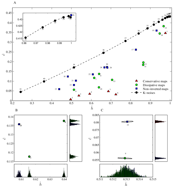
Figure 1: A) Localization in the permutation Lempel–Ziv complexity vs permutation Shannon entropy plane of the chaotic series and $K$-noise series considered in the present work, for the parameters $d=5$ and $\tau=1$. For each case, we generated $N=4.10^{4}$ times series of $L=10^{6}$ samples, initializing each of them randomly. The labels corresponds to that of section 4. All chaotic maps are clearly separate from the $K$-noises. B-C) Zoom in a zone containing the coordinates for specifics chaotic maps. The inferior and lateral plots depict the corresponding histograms of the values taken by each measure separately using the $N=4.10^{6}$ snapshots. The ellipses corresponding to the standard deviation are small. Similar result are obtained for the parameters $d=4,6$ and $\tau=1$

5.2 $K$-noises, FBM and FGN analysis

Let us now analyze the permutation Lempel–Ziv complexity vs the permutation Shannon entropy for the $K$-noises, FBM and FGN time series for various values of $k$ or $H$. To this aim, we generated $N=4.10^{4}$ series of noise, of length $L=10^{6}$ samples each. For the nonGaussian $K$–noises we used the parameter $k\in[0\,;\,3.5]$, for the FBM and FGN series the Hurst exponent $H$ is in $(0,1)$ and the Bandt–Pompe symbolization parameter used for all the series are $d=5$ and $\tau=1$. Figure 2 depicts the mean values of ($\widehat{c},~{}\widehat{h}$) over the realizations, for the each sequences.

As observed in Figure 1, the complexity-entropy points of the sequences of the $K$-noises spread along straight line. As intuitively expected, signal with low correlation stay in the high entropy and complexity values, as zoomed also in the insert of figure 2. This effect remains for FBM sequences, but is no more valid for the FGN; such a behavior remain to be more deeply analyzed. An interesting feature is that the points corresponding to the FBM processes and $K$-noise remain in an intermediate-high region on the complexity-entropy plane while that corresponding to the FGN are concentrated in an high region of the plane. In particular, given a spectrum (power-law exponent), the three types of noise are clearly separated, which is obviously impossible by the mean of a usual spectral analysis. This lets suggest that more than the statistics (Gaussian vs nonGaussian) and more than the stationarity are captured by the couple of measures proposed here.

Note that for the FGN, as $\min(H,1-H)$ increases, the absolute value of the correlation increases, behavior that is conserved in terms of permutation entropy and permutation complexity. However, the permutation entropy given by $H$ and $1-H$ are more or less identical. In other words, such an entropy is unable to distinguish whether correlation or anticorrelation characterizes the underlying FBM process. This is revealed by the permutation Lempel–Ziv complexity (see the insert of figure 2). In other words, the permutation Lempel–Ziv complexity capture the short-range correlation, or persistency vs non-persistency. This effect strengthens the importance of using two different “complementary” measures to analyze such random sequences.

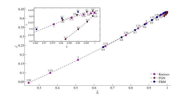
Figure 2: Localization in the permutation Lempel–Ziv complexity vs permutation Shannon entropy plane of $K$-noise, FGN and FBM sequences. The $K$-noises were generated using the parameter $K=0.25m,\,m=1,\ldots,3.5$. For the FGN and FBM we use the Hurst exponent $H=0.1n,\,n=1,...,9$ . For each time series we generated $N=4.10^{4}$ times series of $L=10^{6}$ samples. The corresponding Bandt-Pompe parameter were $d=5$ and $\tau=1$. The same kind of figure are obtained for the parameter $d=4,6$ and $\tau=1$.

6 Discussion

In the analysis of time series, the challenge of distinguishing chaotic dynamics from stochastic dynamics underlying an (apparently) complex time series could be a critical and subtle issue. Numerous tools and methods that attempt to solve such as challenge can be found in the literature: from information theoretic tools that address such a problem from a statistics point of view to deterministic analysis based on the notion of complexity in the sense of Kolmogorov. In this paper, we proposed to analyze time series in a complexity–entropy plane. The idea is to combine both statistical and deterministic/algorithmic point of views.

To use these two measures in their natural discrete-state framework, the signals must be previously quantized. In our approach, the quantization is based on permutation vectors following the scheme proposed by Bandt and Pompe dealing with the so-called permutation entropy.

The Shannon entropy and the Lempel–Ziv complexity applied to the permutation vectors result in the so-called permutation Shannon entropy and permutation Lempel–Ziv complexity respectively. We use the hence defined complexity-entropy plane to analyze several well known time series of the literature –chaotic maps, $K$-noises, fractional Brownian motion and fractional Gaussian noise. In particular, the proposed representation allows to clearly distinguish chaotic maps from random processes, to classify the chaotic maps according to their “non inverted”, “dissipative”and “conservative” characteristics, or to separate noise sharing the same spectrum capturing implicitly both their statistics and their stationarity/nonstationarity. Such a plane appears thus to be a good alternative or complement of the already proposed maps.

As future direction of investigation, the maps proposed in the literature should be compared through automatic classification approaches. One can also imagine to combine three measures to capture more complementary aspects rather than only “permutation” statistical and algorithmic aspects, without a too complex estimation/evaluation procedure. Similarly, rather than Shannon entropy, generalized entropy may be able to capture finer statistical aspects (e.g.,the tails of head of distribution via Rényi-Tsallis entropies).

References

- [1] S. Zozor, O. Blanc, V. Jacquemet, N. Virag, J.-M. Vesin, E. Pruvot, L. Kappenberger, and C. Henriquez. A numerical scheme for modeling wavefront propagation on a monolayer of arbitrary geometry. IEEE Transactions on Biomedical Engineering, 50(4):412–420, April 2003.
- [2] N. Kannathal, S. K. Puthusserypady, and L. C. Min. Complex dynamics of epileptic EEG. In Proc. of the 26th Annual International Conference of the IEEE Engineering in Medicine and Biology Society (EMBS’04), volume 1, pages 604–607, San Fransisco, CA, USA, September 1-5 2004. IEEE.
- [3] W. B. Arthur. Inductive reasoning and bounded rationality. The American Economic Review, 84(2):406–411, May 1994.
- [4] N. B. Tuma. Social Dynamics Models and methods. Elsevier, 1984.
- [5] R. J. Shiller, S. Fischer, and B. M. Friedman. Stock prices and social dynamics. Brookings papers on economic activity, 15(2):457–510, 1984.
- [6] M. Rajković. Extracting meaningful information from financial data. Physica A, 287(3-4):383–395, December 2000.
- [7] V. I. Ponomarenko and M. D. Prokhorov. Extracting information masked by the chaotic signal of a time-delay system. Physical Review E, 66(2):026215, August 2002.
- [8] D. S. Broomhead and G. P. King. Extracting qualitative dynamics from experimental data. Physica D, 20(2-3):217–236, June-July 1986.
- [9] R. Quian Quiroga, J. Arnhold, K. Lehnertz, and P. Grassberger. Kulback–Leibler and renormalized entropies: Applications to electroencephalograms of epilepsy patients. Physical Review E, 62(6):8380–8386, December 2000.
- [10] O. A. Rosso, S. Blanco, J. Yordanova, V. Kolev, A. Figliola, M. Schürmann, and E. Başar. Wavelet entropy: a new tool for analysis of short duration brain electrical signals. Journal of neuroscience methods, 105(1):65–75, January 2001.
- [11] T. Schreiber. Measuring information transfer. Physical Review Letters, 85(2):461–464, July 2000.
- [12] A. Wolf, J. B. Swift, H. L. Swinney, and J. A. Vastano. Determining Lyapunov exponents from a time series. Physica D, 16(3):285–317, July 1985.
- [13] R. Nagarajan. Quantifying physiological data with lempel-ziv complexity-certain issues. Biomedical Engineering, IEEE Transactions on, 49(11):1371–1373, 2002.
- [14] M. Aboy, R. Hornero, D. Abásolo, and D. Álvarez. Interpretation of the Lempel-Ziv complexity measure in the context of biomedical signal analysis. IEEE Transactions on Biomedical Engineering, 53(11):2282–2288, November 2006.
- [15] S. Zozor, P. Ravier, and O. Buttelli. On Lempel–Ziv complexity for multidimensional data analysis. Physica A, 345(1-2):285–302, January 2005.
- [16] C. Vignat and J.-F. Bercher. Analysis of signals in the Fisher-Shannon information plane. Physics Letters A, 312(1-2):27–33, June 2003.
- [17] O. A. Rosso, H. A. Larrondo, M. T. Martin, A. Plastino, and M. A. Fuentes. Distinguishing noise from chaos. Physical Review Letters, 99(15):154102, October 2007.
- [18] O. A. Rosso, F. Olivares, L. Zunino, L. De Micco, A. L. L. Aquino, A. Plastino, and H. A. Larrondo. Characterization of chaotic maps using the permutation Bandt–Pompe probability-distribution. The European Physics Journal B, 86(4):116–128, april 2013.
- [19] O. A. Rosso, H. Craig, and P. Moscato. Shakespeare and other English renaissance authors as characterized by information theory complexity quantifiers. Physica A, 388(6):916–926, March 2009.
- [20] L. Zunino, M. C. Soriano, I. Fischer, O. A. Rosso, and C. R. Mirasso. Permutation-information-theory approach to unveil delay dynamics from time-series analysis. Physical Review E, 82(4):046212, October 2010.
- [21] F. Montani and O. A. Rosso. Entropy-complexity characterization of brain development in chickens. Entropy, 16(8):4677–4692, 2014.
- [22] P. W. Lamberti, M. T. Martin, A. Plastino, and O. A. Rosso. Intensive entropic non-triviality measure. Physica A, 334(1-2):119–131, March 2004.
- [23] A. Lempel and J. Ziv. On the complexity of finite sequences. IEEE Transactions on Information Theory, 22(1):75–81, January 1976.
- [24] C. E. Shannon. A mathematical theory of communication. The Bell System Technical Journal, 27(4):623–656, October 1948.
- [25] J. Beirlant, E. J. Dudewicz, L. Györfi, and E. C. van der Meulen. Nonparametric entropy estimation: An overview. International Journal of Mathematical and Statistical Sciences, 6(1):17–39, June 1997.
- [26] N. Leonenko, L. Pronzato, and V. Savani. A class of Rényi information estimators for multidimensional densities. Annals of Statistics, 36(5):2153–2182, October 2008.
- [27] T. Schürmann and P. Grassberger. Entropy estimation of symbol sequences. Chaos, 6(3):414, September 1996.
- [28] A. O. Hero III, B. Ma, O. J. J. Michel, and J. Gorman. Application of entropic spanning graphs. IEEE Signal Processing Magazine, 19(5):85–95, September 2002.
- [29] S. Frenzel and B. Pompe. Partial mutual information for coupling analysis of multivariate time series. Physical Review Letters, 99(20):204101, November 2007.
- [30] M. Rosenblatt. Remarks on some nonparametric estimates of a density function. The Annals of Mathematical Statistics, 27(3):832–837, September 1956.
- [31] E. Parzen. On estimation of a probability density function and mode. The Annals of Mathematical Statistics, 33(3):1065–1076, September 1962.
- [32] C. Bandt and B. Pompe. Permutation entropy: A natural complexity measure for time series. Physical Review Letters, 88(17):174102, April 2002.
- [33] S. Zozor, D. Mateos, and P. W. Lamberti. Mixing Bandt–Pompe and Lempel–Ziv approaches: another way to analyze the complexity of continuous-states sequences. The European Physical Journal B, 87(5):107, May 2014.
- [34] L. Boltzmann (translated by Stephen G. Brush). Lectures on Gas Theory. Dover, Leipzig, Germany, 1964.
- [35] J. W. Gibbs. Elementary Principle in Statistical Mechanics. University Press - John Wilson and son, Cambridge, USA, 1902.
- [36] J. von Neumann. Thermodynamik quantenmechanischer gesamtheiten. Nachrichten von der Gesellschaft der Wissenschaften zu Göttingen, 1:273–291, 1927.
- [37] F. R. S. W. D. Nieven, M. A. The scientific papers of James Clerk Maxwell, volume 2. Dover, New-York, 1952.
- [38] E. T. Jaynes. Gibbs vs Boltzmann entropies. American Journal of Physics, 33(5):391–398, May 1965.
- [39] I. Müller and W. H. Müller. Fundamentals of Thermodynamics and Applications. With Historical Annotations and Many Citations from Avogadro to Zermelo. Springer, Berlin, 2009.
- [40] M. Planck. Eight Lectures on Theoretical Physics. Columbia University Press, New-York, 2015.
- [41] A. I. Khinchin. Mathematical foundations of information theory. Dover Publications, New-York, 1957.
- [42] T. M. Cover and J. A. Thomas. Elements of Information Theory. John Wiley & Sons, Hoboken, New Jersey, 2nd edition, 2006.
- [43] R. L. Dobrushin. A simplified method of experimentally evaluating the entropy of a stationary sequences. Theory of Probability and its Applications, 3(4):428–430, 1958.
- [44] O. Vasicek. A test for normality based on sample entropy. Journal of the Royal Statistical Society B, 38(1):54–59, 1976.
- [45] L. F. Kozachencko and N. N. Leonenko. Sample estimate of the entropy of a random vector. Problems in Information transmission, 23(2):95–101, 1987.
- [46] J. Ziv and A. Lempel. A universal algorithm for sequential data compression. IEEE Transactions on Information Theory, 23(3):337–343, May 1977.
- [47] J. Ziv and A. Lempel. Compression of individual sequences via variable-rate coding. IEEE Transactions on Information Theory, 24(5):530–536, September 1978.
- [48] A. D. Wyner and J. Ziv. Some asymptotic properties of the entropy of a stationary ergodic data source with applications to data compression. IEEE Transactions on Information Theory, 35(6):1250–1258, november 1989.
- [49] G. Hansel. Estimation of the entropy by the Lempel-Ziv method. Lecture Notes in Computer Science (Electronic Dictionaries and Automata in Computational Linguistics), 377:51–65, 1989.
- [50] F. Kaspar and H. G. Schuster. Easily calculable measure for the complexity of spatiotemporal patterns. Physical Review A, 36(2):842–848, July 1987.
- [51] F. Takens. Detecting strange attractors in turbulence. In D. Rand and L.-S. Young, editors, Dynamical Systems and Turbulence, volume 898 of Lecture Notes in Mathematics, pages 366–383. Springer Verlag, Warwick, 1981.
- [52] J. C. Robinson. Dimensions, Embeddings, and Attractors. Cambridge University Press, Cambdrige, UK, 2011.
- [53] A. Gersho and R. M. Gray. Vector quantization and signal compression. Kluwer, Boston, 1992.
- [54] J. M. Amigó, L. Kocarev, and J. Szczepanski. Order patterns and chaos. Physics Letters A, 355(1):27–31, June 2006.
- [55] J. M. Amigó. Permutation Complexity in Dynamical Systems. Springer Verlag, Heidelberg, 2010.
- [56] J. M. Amigó, S. Zambrano, and M. A. F. Sanjuán. True and false forbidden patterns in deterministic and random dynamics. Europhysics Letters, 79(5):50001, September 2007.
- [57] O. A. Rosso, L. C. Carpi, P. M. Saco, and M. Gómez Ravetti. Causality and the entropy-complexity plane: Robustness and missing ordinal patterns. Physica A, 391(1-2):42–45, january 2012.
- [58] J.C. Sprott. Chaos and time-series analysis. Oxford University Press, Oxford, 2003.
- [59] P. Dutta and P. M. Horn. Low-frequency fluctuations in solids: noises. Reviews of Modern Physics, 53(3):497–516, July 1981.
- [60] J. R. M. Hosking. Fractional differencing. Biometrika, 68(1):165–176, April 1981.
- [61] B. West and M. Shlesinger. The noise in natural phenomena. American Scientist, 78(1):40–45, January-February 1990.
- [62] A. N. Kolmogorov. Sienersche spiralen und einige andere interessante kurven im hilbertschen raum. Doklady Akademii nauk SSSR, 26(2):115–118, 1940.
- [63] H. Hurst. Long-term storage capacity in reservoirs. Transactions of the American Society of Civil Engeniering, 116:770–799, 1951.
- [64] B. Mandelbrot and J. W. Van Ness. Fractional Brownian motions, fractional noises and applications. SIAM review, 10(4):422–437, October 1968.
- [65] P. Flandrin. On the spectrum of fractional Brownian motions. IEEE Transactions on Information Theory, 35(1):197–199, January 1989.
- [66] L. Zunino, D. .G Pérez, M. T. Martín, A. Plastino, M. Garavaglia, and O. A. Rosso. Characterization of Gaussian self-similar stochastic processes using wavelet-based informational tools. Physical Review E, 75(2):021115, February 2007.
- [67] J. Beran. Statistics for Long-Memory Processes. Chapman & Hall, New-York, 1994.
- [68] G. Samorodnitsky and M. S. Taqqu. Stable Non-Gaussian Random Processes. Stochastic Models with infinite Variance. Chapman & Hall, New-York, 1994.
- [69] J. Feder. Fractals, volume 9. Springer, New-York, 1988.
- [70] F. J. Molz, H. H. Lui, and J. Szulga. Fractional Brownian motion and fractional Gaussian noise in subsurface hydrology: A review, presentation of fundamental properties, and extensions. Water Resources Research, 33(10):2273–2286, October 1997.
- [71] G. Samorodnitsky. Long range dependence. Foundations and Trends in Stochastic Systems, 1(3):163–257, 2007.
- [72] R. B. Davies and D. S. Harte. Tests for Hurst effect. Biometrika, 74(1):95–101, March 1987.
- [73] P. Abry and F. Sellan. The wavelet-based synthesis for fractional Brownian motion proposed by f. sellan and y. meyer: Remarks and fast implementation. Applied and Computational Harmonic Analysis, 3(4):377–383, October 1996.
- [74] W. Kinzel and G. Reents. Physics by Computers – Programming Physical Problems Using Mathematica and C. Springer Verlag, Heidelberg, 1998.