Existence of Static Wormholes in $f(\mathcal{G},T)$ Gravity

Abstract

This paper investigates static spherically symmetric traversable wormhole solutions in $f(\mathcal{G},T)$ gravity ($\mathcal{G}$ and $T$ represent the Gauss-Bonnet invariant and trace of the energy-momentum tensor, respectively). We construct explicit expressions for ordinary matter by taking specific form of red-shift function and $f(\mathcal{G},T)$ model. To analyze possible existence of wormholes, we consider anisotropic, isotropic as well as barotropic matter distributions. The graphical analysis shows the violation of null energy condition for the effective energy-momentum tensor throughout the evolution while ordinary matter meets energy constraints in certain regions for each case of matter distribution. It is concluded that traversable WH solutions are physically acceptable in this theory.

Keywords: Wormhole solutions; $f(\mathcal{G},T)$ gravity.
PACS: 04.50.Kd; 95.36.+x.

1 Introduction

Gauss-Bonnet (GB) invariant has a significant importance in higher dimensional theories as well as in describing the early and late-times cosmic evolution. It is a quadratic curvature invariant of the form $\mathcal{G}=R_{\alpha\beta\gamma\delta}R^{\alpha\beta\gamma\delta}-4R_{\alpha\beta}R^{\alpha\beta}+R^{2}$, where $R_{\alpha\beta\gamma\delta},~{}R_{\alpha\beta}$ and $R$ represent the Riemann tensor, Ricci tensor and Ricci scalar, respectively. This quadratic invariant is a four-dimensional topological term and is free from spin-2 ghost instabilities [1]. Nojiri and Odintsov [2] added the generic function $f(\mathcal{G})$ in the Einstein-Hilbert action (dubbed as $f(\mathcal{G})$ gravity) to explore the dynamics of GB invariant in four dimensions. This modified theory is consistent with solar system constraints as well as endowed with a quite rich cosmological structure [3]. It is interesting to investigate the effects of non-minimal coupling between curvature and matter on cosmic evolution. Recently, we have established this curvature-matter coupling in the action of $f(\mathcal{G})$ gravity named as $f(\mathcal{G},T)$ gravity [4]. We have found that energy-momentum tensor is not conserved due to the presence of non-minimally curvature-matter coupling. This non-conservation produces an extra force due to which dust particles move along geodesic lines of geometry while non-geodesic trajectories are followed by massive particles. The background of cosmological evolutionary models corresponding to phantom/non-phantom eras, power-law solutions as well as de Sitter universe can be discussed in this theory [5].

A wormhole (WH) is defined as a hypothetical bridge or tunnel that provides a shortcut across the spacetime for long distances. Inter-universe WH allows a path of communication between distant patches of distinct spacetimes while a subway connecting distant regions of the same spacetime is dubbed as an intra-universe WH. The simplest solution of the Einstein field equations representing this hypothetical connecting shortcut is Schwarzschild WH also known as Einstein-Rosen bridge [6]. Schwarzschild WH does not allow two-way travel (non-traversable WH) due to the presence of strong tidal gravitational forces at WH throat which would destroy anything that tries to pass through. Moreover, it evolves with time such that expansion (circumference increases from zero to finite) and contraction (shrinks to zero) of WH throat are very rapid and it does not allow anything to pass through the tunnel. Schwarzschild WH possesses highly unstable antihorizon that changes to a horizon even when light passes through it, thereby closing the WH throat. To overcome these drawbacks, Morris and Thorne [7] gave the concept of traversable WHs. They observed that these WHs must be sustained by the matter which violates the null energy condition (NEC) dubbed as exotic matter. The presence of this unrealistic form of matter pushes the walls of WH apart and prevents the WH throat to shrink.

The search for alternative source of violation such that ordinary matter meets the energy conditions has always been a subject of great interest. Brane WHs, dynamical WH solutions, non-commutative geometry, generalized Chaplygin gas, modified theories of gravity, etc provide a source that helps to minimize the usage of exotic matter to support the WH geometry [8]. In modified theories of gravity, the effective energy-momentum tensor (includes higher-curvature terms and ordinary matter variables) acts as a source of violation required for the traversability and thus provides a possibility for the existence of realistic WH. Furey and DeBenedicts [9] investigated WH solutions for $R^{2}$ and $R^{-1}$ theories of gravity and found the positivity of weak energy condition (WEC) in the neighborhood of WH throat. Lobo and Oliveira [10] discussed static spherically symmetric WH solutions and found that realistic WH geometries threaded by ordinary matter can be formed in $f(R)$ gravity.

Azizi [11] explored WH geometries and found that NEC is satisfied for barotropic matter configuration in $f(R,T)$ gravity. The physically acceptable WH solutions are observed for barotropic fluid in the background of $f(R)$ gravity [12]. Sharif and Rani [13] studied static spherically symmetric WH solutions for exponential as well as logarithmic forms of generalized teleparallel gravity and found that WEC is violated in galactic halo region for both models. Mehdizadeh et al. [14] discussed realistic traversable WH solutions in Einstein GB gravity. We have explored WH geometries for traceless, isotropic as well as barotropic matter distributions and concluded that realistic WH solutions exist in $f(\mathcal{G})$ gravity only for radial barotropic fluid [15]. Zubair and his collaborators [16] investigated WH solutions and found that stable physically acceptable WH solutions exist for anisotropic matter configuration.

In this paper, we explore static spherically symmetric WH solutions for anisotropic, isotropic and barobropic matter distributions in $f(\mathcal{G},T)$ gravity. The paper has the following format. In the next section, we discuss basic concepts related to $f(\mathcal{G},T)$ gravity, WH geometry as well as energy conditions. Section 3 is devoted to construct WH solutions using three types of fluid for specific $f(\mathcal{G},T)$ model. In section 4, we summarize the results.

2 Field Equations for Wormhole Construction

The action for $f(\mathcal{G},T)$ gravity is defined as [4]

$$\mathcal{I}=\int\left(\frac{R+f(\mathcal{G},T)}{2\kappa^{2}}+\mathcal{L}_{m}\right)\sqrt{-g}d^{4}x,$$ (1)

where $\mathcal{L}_{m},~{}\kappa^{2}$ and $g$ denote the Lagrangian density associated with matter configuration, coupling constant and determinant of the metric tensor, respectively. Varying the action (1) with respect to $g_{\alpha\beta}$, we obtain the fourth order field equations as follows

$$G_{\alpha\beta}=\kappa^{2}T_{\alpha\beta}^{\mathrm{eff}}=\kappa^{2}(T_{\alpha\beta}+T_{\alpha\beta}^{\mathcal{G}T}),$$ (2)

where $G_{\alpha\beta}$ and $T_{\alpha\beta}^{\mathrm{eff}}$ represent Einstein tensor and effective energy-momentum tensor, respectively. The expression for $T_{\alpha\beta}^{\mathcal{G}T}$ is given by

$$\kappa^{2}T_{\alpha\beta}^{\mathcal{G}T} = \frac{1}{2}g_{\alpha\beta}f(\mathcal{G},T)-T_{\alpha\beta}f_{T}(\mathcal{G},T)-\Theta_{\alpha\beta}f_{T}(\mathcal{G},T)-2RR_{\alpha\beta}f_{\mathcal{G}}(\mathcal{G},T)$$

$$+ 4R_{\alpha}^{~{}\zeta}R_{\zeta\beta}f_{\mathcal{G}}(\mathcal{G},T)+4R_{\alpha\gamma\beta\delta}R^{\gamma\delta}f_{\mathcal{G}}(\mathcal{G},T)-2R_{\alpha}^{~{}\gamma\delta\zeta}R_{\beta\gamma\delta\zeta}f_{\mathcal{G}}(\mathcal{G},T)$$

$$- 2Rg_{\alpha\beta}\Box f_{\mathcal{G}}(\mathcal{G},T)-4R_{\alpha}^{~{}\zeta}\nabla_{\beta}\nabla_{\zeta}f_{\mathcal{G}}(\mathcal{G},T)-4R_{\beta}^{~{}\zeta}\nabla_{\alpha}\nabla_{\zeta}f_{\mathcal{G}}(\mathcal{G},T)$$

$$+ 2R\nabla_{\alpha}\nabla_{\beta}f_{\mathcal{G}}(\mathcal{G},T)+4g_{\alpha\beta}R^{\gamma\delta}\nabla_{\gamma}\nabla_{\delta}f_{\mathcal{G}}(\mathcal{G},T)+4R_{\alpha\beta}\Box f_{\mathcal{G}}(\mathcal{G},T)$$

$$- 4R_{\alpha\gamma\beta\delta}\nabla^{\gamma}\nabla^{\delta}f_{\mathcal{G}}(\mathcal{G},T),$$

where $f_{T}(\mathcal{G},T)=\partial f(\mathcal{G},T)/\partial T,~{}f_{\mathcal{G}}(\mathcal{G},T)=\partial f(\mathcal{G},T)/\partial\mathcal{G},~{}\Box=\nabla^{2}=\nabla_{\alpha}\nabla^{\alpha}$ and $\nabla_{\alpha}$ is a covariant derivative whereas tensor $\Theta_{\alpha\beta}$ has the form [17]

$$\Theta_{\alpha\beta}=g^{\gamma\zeta}\frac{\delta T_{\gamma\zeta}}{\delta g_{\alpha\beta}}=g_{\alpha\beta}\mathcal{L}_{m}-2g^{\gamma\zeta}\frac{\partial^{2}\mathcal{L}_{m}}{\partial g^{\alpha\beta}\partial g^{\gamma\zeta}}-2T_{\alpha\beta},$$

with the assumption that the matter Lagrangian density depends only on $g_{\alpha\beta}$. The energy-momentum tensor for anisotropic matter distribution is

$$T_{\alpha\beta}=(\rho+P_{t})u_{\alpha}u_{\beta}-P_{t}g_{\alpha\beta}+(P_{r}-P_{t})\eta_{\alpha}\eta_{\beta},$$ (3)

where $u_{\alpha},~{}\eta_{\alpha},~{}\rho,~{}P_{r}$ and $P_{t}$ represent the four velocity, unit four-vector in radial direction, energy density, radial and tangential pressures of the fluid, respectively. For anisotropic configuration, we take $\mathcal{L}_{m}=\rho$, the resultant expression for $\Theta_{\alpha\beta}$ becomes

$$\Theta_{\alpha\beta}=\rho g_{\alpha\beta}-2T_{\alpha\beta}.$$ (4)

The static spherically symmetric line element describing the geometry of traversable WH is given by [7]

$$ds^{2}=e^{2\psi(r)}dt^{2}-\left(1-\frac{\chi(r)}{r}\right)^{-1}dr^{2}-r^{2}d\theta^{2}-r^{2}\sin^{2}\theta d\phi^{2},$$ (5)

where $\psi(r)$ and $\chi(r)$ are the generic functions of $r$ known as red-shift and shape functions, respectively. The first function $\psi(r)$ measures the magnitude of gravitational red-shift of a photon while geometry of WH is determined by $\chi(r)$. For the traversability of WH, $\psi(r)$ must be finite everywhere to satisfy the no-horizon condition. The shape function must represent the increasing behavior with respect to $r$ such that $(1-\chi(r)/r)>0$ throughout the tunnel to maintain the WH geometry. In addition, the value of $\chi(r)$ and $r$ must be same at throat, i.e., $\chi(r_{\mathrm{th}})=r_{\mathrm{th}}$. The fundamental condition known as flaring-out condition, given by $(\psi(r)-\psi^{\prime}(r)r)/\psi^{2}(r)>0$, needs to be satisfied throughout the evolution while the constraint $\chi^{\prime}(r_{\mathrm{th}})<1$ should be imposed at the throat. Also, the asymptotically flatness condition, $\chi(r)/r\rightarrow 0$ as $r\rightarrow\infty$, must be fulfilled.

Using Eqs.(3)-(5) in (2), we obtain the following set of field equations

$$\kappa^{2}\rho = \frac{\chi^{\prime}}{r^{2}}-\frac{1}{2}f(\mathcal{G},T)+\frac{1}{2}\mathcal{G}f_{\mathcal{G}}(\mathcal{G},T)+\frac{2}{r^{4}}(r\chi^{\prime}-\chi)\left(2-\frac{3\chi}{r}\right)f_{\mathcal{G}}^{\prime}(\mathcal{G},T)$$ (6)

$$+ \frac{4\chi}{r^{3}}\left(1-\frac{\chi}{r}\right)f_{\mathcal{G}}^{\prime\prime}(\mathcal{G},T),$$

$$\kappa^{2}P_{r} = \left[\frac{2\psi^{\prime}}{r}\left(1-\frac{\chi}{r}\right)-\frac{\chi}{r^{3}}+\frac{1}{2}f(\mathcal{G},T)-\frac{1}{2}\mathcal{G}f_{\mathcal{G}}(\mathcal{G},T)-\frac{4\psi^{\prime}}{r^{3}}(3\chi-2r)\right.$$ (7)

$$\times \left.\left(1-\frac{\chi}{r}\right)f_{\mathcal{G}}^{\prime}(\mathcal{G},T)-\rho f_{T}(\mathcal{G},T)\right]\left(1+\frac{f_{T}(\mathcal{G},T)}{\kappa^{2}}\right)^{-1},$$

$$\kappa^{2}P_{t} = \left[\left(\frac{\psi^{\prime}}{r}+\psi^{\prime 2}+\psi^{\prime\prime}\right)\left(1-\frac{\chi}{r}\right)+\frac{1}{2r^{3}}(1+r\psi^{\prime})(\chi-\chi^{\prime}r)+\frac{1}{2}f(\mathcal{G},T)\right.$$ (8)

$$- \left.\frac{1}{2}\mathcal{G}f_{\mathcal{G}}(\mathcal{G},T)+\frac{2}{r}\left(1-\frac{\chi}{r}\right)\left\{2(\psi^{\prime 2}+\psi^{\prime\prime})\left(1-\frac{\chi}{r}\right)-\frac{3\psi^{\prime}}{r^{2}}(\chi^{\prime}r\right.\right.$$

$$- \left.\left.\chi)\right\}f_{\mathcal{G}}^{\prime}(\mathcal{G},T)+\frac{4\psi^{\prime}}{r}\left(1-\frac{\chi}{r}\right)^{2}f_{\mathcal{G}}^{\prime\prime}(\mathcal{G},T)-\rho f_{T}(\mathcal{G},T)\right]$$

$$\times \left(1+\frac{f_{T}(\mathcal{G},T)}{\kappa^{2}}\right)^{-1},$$

where prime is the derivative with respect to $r$ and $T=\rho-P_{r}-2P_{t}$ whereas GB invariant has the following expression

$$\mathcal{G}=\frac{4}{r^{4}}\left[\psi^{\prime}(\chi-\chi^{\prime}r)\left(2-\frac{3\chi}{r}\right)-2r\chi(\psi^{\prime 2}+\psi^{\prime\prime})\left(1-\frac{\chi}{r}\right)\right].$$ (9)

The above system of equations (6)-(8) shows that the generic function $f(\mathcal{G},T)$ has a direct dependence on matter variables therefore, it would be difficult to find the explicit expressions for $\rho,~{}P_{r}$ and $P_{t}$. The favorable approach to solve this system for matter contents is to choose $f(\mathcal{G},T)=F(\mathcal{G})+\mathcal{F}(T)$ with $\mathcal{F}(T)=\Upsilon T$, where $\Upsilon$ is an arbitrary constant. This simplest choice of $f(\mathcal{G},T)$ function does not involve the direct curvature-matter non-minimally coupling and is considered as the correction to $f(\mathcal{G})$ gravity. For this particular $f(\mathcal{G},T)$ form, we simplify the equations (6)-(8) as follows

$$\rho = \frac{1}{2(1+2\Upsilon)}\left[\left(\frac{2+5\Upsilon}{1+\Upsilon}\right)\Omega_{1}+\Upsilon(\Omega_{2}+2\Omega_{3})\right],$$ (10)

$$P_{r} = \frac{-1}{2(1+2\Upsilon)}\left[\left(\frac{\Upsilon}{1+\Upsilon}\right)\Omega_{1}-(2+3\Upsilon)\Omega_{2}+2\Upsilon\Omega_{3}\right],$$ (11)

$$P_{t} = \frac{-1}{2(1+\Upsilon)(1+2\Upsilon)}\left[\Upsilon\Omega_{1}+\Upsilon(1-\Upsilon)\Omega_{2}+2(1-\Upsilon)^{2}\Omega_{3}\right],$$ (12)

where $\kappa^{2}=1$ and

$$\Omega_{1} = \frac{\chi^{\prime}}{r^{2}}-\frac{1}{2}F(\mathcal{G})+\frac{1}{2}\mathcal{G}F_{\mathcal{G}}(\mathcal{G})+\frac{2}{r^{4}}(r\chi^{\prime}-\chi)\left(2-\frac{3\chi}{r}\right)F_{\mathcal{G}}^{\prime}(\mathcal{G})$$

$$+ \frac{4\chi}{r^{3}}\left(1-\frac{\chi}{r}\right)F_{\mathcal{G}}^{\prime\prime}(\mathcal{G}),$$

$$\Omega_{2} = \frac{1}{(1+\Upsilon)}\left[\frac{2\psi^{\prime}}{r}\left(1-\frac{\chi}{r}\right)-\frac{\chi}{r^{3}}+\frac{1}{2}F(\mathcal{G})-\frac{1}{2}\mathcal{G}F_{\mathcal{G}}(\mathcal{G})-\frac{4\psi^{\prime}}{r^{3}}(3\chi-2r)\right.$$

$$\times \left.\left(1-\frac{\chi}{r}\right)F_{\mathcal{G}}^{\prime}(\mathcal{G})\right],$$

$$\Omega_{3} = \frac{1}{(1+\Upsilon)}\left[\left(\frac{\psi^{\prime}}{r}+\psi^{\prime 2}+\psi^{\prime\prime}\right)\left(1-\frac{\chi}{r}\right)+\frac{1}{2r^{3}}(1+r\psi^{\prime})(\chi-\chi^{\prime}r)\right.$$

$$+ \left.\frac{1}{2}F(\mathcal{G})-\frac{1}{2}\mathcal{G}F_{\mathcal{G}}(\mathcal{G})+\frac{2}{r}\left(1-\frac{\chi}{r}\right)\left\{2(\psi^{\prime 2}+\psi^{\prime\prime})\left(1-\frac{\chi}{r}\right)-\frac{3\psi^{\prime}}{r^{2}}\right.\right.$$

$$\times \left.\left.(\chi^{\prime}r-\chi)\right\}F_{\mathcal{G}}^{\prime}(\mathcal{G})+\frac{4\psi^{\prime}}{r}\left(1-\frac{\chi}{r}\right)^{2}F_{\mathcal{G}}^{\prime\prime}(\mathcal{G})\right].$$

It is worth mentioning here that the above equations reduce to $f(\mathcal{G})$ gravity for $\Upsilon=0$ while general relativity (GR) is recovered when the contribution of generic function vanishes, i.e., $F(\mathcal{G})=0$ with $\Upsilon=0$ [15].

Energy conditions are used to discuss physically realistic matter configuration that are originated from Raychaudhuri equations. These constraints are imposed on the energy-momentum tensor and possess an interesting feature that they are coordinate invariant. The Raychaudhuri equations describe the temporal evolution of expansion scalar $(\theta)$ for the congruences of timelike $(v^{\alpha})$ and null $(l_{\alpha}$) geodesics as [18]

$$\frac{d\theta}{d\tau}-\omega_{\alpha\beta}\omega^{\alpha\beta}+\sigma_{\alpha\beta}\sigma^{\alpha\beta}+\frac{1}{3}\theta^{2}+R_{\alpha\beta}v^{\alpha}v^{\beta}=0,$$

$$\frac{d\theta}{d\tau}-\omega_{\alpha\beta}\omega^{\alpha\beta}+\sigma_{\alpha\beta}\sigma^{\alpha\beta}+\frac{1}{2}\theta^{2}+R_{\alpha\beta}l^{\alpha}l^{\beta}=0,$$

where $\omega_{\alpha\beta}$ and $\sigma_{\alpha\beta}$ represent the rotation and shear tensors, respectively. For non-geodesic (timelike or null) congruences, the temporal evolution for expansion scalar changes in the presence of acceleration term as [19]

$$\frac{d\theta}{d\tau}-\omega_{\alpha\beta}\omega^{\alpha\beta}+\sigma_{\alpha\beta}\sigma^{\alpha\beta}+\frac{1}{3}\theta^{2}+R_{\alpha\beta}v^{\alpha}v^{\beta}-\mathcal{A}=0,$$ (13)

the auxiliary term $\mathcal{A}=\nabla_{\alpha}(u^{\beta}\nabla_{\beta}u^{\alpha})$ represents divergence of four-acceleration dubbed as acceleration term which appears due to the non-gravitational force (pressure gradient). Using the condition of attractive nature of gravity ($\theta<0$) and neglecting the quadratic terms, the Raychaudhuri equations for non-geodesic congruences reduce to

$$R_{\alpha\beta}v^{\alpha}v^{\beta}-\mathcal{A}\geq 0,\quad R_{\alpha\beta}l^{\alpha}l^{\beta}-\mathcal{A}\geq 0.$$

In terms of energy-momentum tensor, the above inequalities take the form

$$\left(T_{\alpha\beta}-\frac{1}{2}g_{\alpha\beta}T\right)v^{\alpha}v^{\beta}-\mathcal{A}\geq 0,\quad\left(T_{\alpha\beta}-\frac{1}{2}g_{\alpha\beta}T\right)l^{\alpha}l^{\beta}-\mathcal{A}\geq 0.$$ (14)

In modified theories of gravity, these inequalities are obtained by replacing $T_{\alpha\beta}$ with $T_{\alpha\beta}^{\mathrm{eff}}$ since Raychaudhuri equations possess purely geometric nature. In $f(\mathcal{G},T)$ gravity, we find that massive test particles follow the non-geodesic trajectories due to the presence of an extra force [4]. The above inequalities (14) with $T_{\alpha\beta}^{\mathrm{eff}}$ provide the null, weak, strong (SEC) and dominant (DEC) energy conditions as

• NEC:$\quad\rho^{\mathrm{eff}}+P_{i}^{\mathrm{eff}}-\mathcal{A}\geq 0,~{}i=1,2,3$,

• WEC:$\quad\rho^{\mathrm{eff}}+P_{i}^{\mathrm{eff}}-\mathcal{A}\geq 0,~{}\rho^{\mathrm{eff}}-\mathcal{A}\geq 0,$

• SEC:$\quad\rho^{\mathrm{eff}}+P_{i}^{\mathrm{eff}}-\mathcal{A}\geq 0,~{}\rho^{\mathrm{eff}}+\sum_{i}P_{i}^{\mathrm{eff}}-\mathcal{A}\geq 0,$

• DEC:$\quad\rho^{\mathrm{eff}}\pm P_{i}^{\mathrm{eff}}-\mathcal{A}\geq 0,~{}\rho^{\mathrm{eff}}-\mathcal{A}\geq 0,$

where $\rho^{\mathrm{eff}}$ and $P^{\mathrm{eff}}$ represent the effective energy density and pressure, respectively. The null energy condition is considered as the fundamental energy bound whose violation leads to the violation of all energy constraints. It is worth mentioning here that the non-geodesic energy bounds in GR can be obtained by replacing $\rho^{\mathrm{eff}}$ and $P^{\mathrm{eff}}$ with usual matter contents $\rho$ and $P$, respectively. In the absence of acceleration term, i.e., for geodesic congruences, one can recover the usual energy conditions in $f(\mathcal{G},T)$ gravity [4].

For the traversability of WH, the basic property is the violation of NEC in GR. This violation prevents the WH throat to shrink and leads to the physically unrealistic WH solutions. The modified theories of gravity provide $T_{\alpha\beta}^{\mathrm{eff}}$ as an alternative source to meet the violation of NEC. In this regard, these theories may have an opportunity for usual matter configuration to fulfil the energy constraints. Using the field equations (2), we obtain NEC in $f(\mathcal{G},T)$ gravity

$$\rho^{\mathrm{eff}}+P_{r}^{\mathrm{eff}}-\mathcal{A}=\left(\frac{r\chi^{\prime}-\chi}{r^{3}}\right)\left(1-\frac{r\psi^{\prime}}{2}\right)-\left(\psi^{\prime 2}+\psi^{\prime\prime}\right)\left(1-\frac{\chi}{r}\right),$$ (15)

where the acceleration term for Eq.(5) is given by

$$\mathcal{A}=\left(1-\frac{\chi}{r}\right)\left[\psi^{\prime\prime}+\psi^{\prime 2}+\frac{2\psi^{\prime}}{r}\right]-\frac{\psi^{\prime}}{2r^{2}}\left(r\chi^{\prime}-\chi\right).$$ (16)

In the absence of acceleration term, the expression (15) becomes identical to $f(\mathcal{G})$ gravity [15].

3 Wormhole Solutions

In this section, we investigate WH solutions by taking three different types of matter distribution for specific form of $\psi(r)$ and viable $F(\mathcal{G})$ model. We assume the finite red-shift function as [20]

$$\psi(r)=-\frac{\lambda}{r},\quad\lambda>0,$$ (17)

which meets the no-horizon condition as well as shows asymptotically flatness behavior at large distances, i.e., $\psi(r)\rightarrow 0$ as $r\rightarrow\infty$. The expression for GB invariant (9) takes the form

$$\mathcal{G}=\frac{4\lambda}{r^{7}}\left[(2r-3\chi)(\chi-r\chi^{\prime})-2\chi(\lambda-2r)\left(1-\frac{\chi}{r}\right)\right].$$ (18)

We consider the following algebraic power-law form as [21]

$$F(\mathcal{G})=\mu\mathcal{G}^{a}(1+\nu\mathcal{G}^{b}),$$ (19)

where $a,~{}b,~{}\mu$ and $\nu$ are arbitrary constants. Under certain conditions on these model parameters, this realistic model does not possess any four types of finite-time future singularities as well as efficiently describes the current cosmic acceleration. Using Eqs.(17) and (19), the expressions for $\Omega_{i}$’s in the field equations (10)-(12) become

$$\Omega_{1} = \frac{\chi^{\prime}}{r^{2}}-\frac{1}{2}\mu\mathcal{G}^{a}(1+\nu\mathcal{G}^{b})+\frac{1}{2}\mu\mathcal{G}^{a}[a+\mu(a+b)\mathcal{G}^{b}]+\frac{2\mu}{r^{4}}(r\chi^{\prime}-\chi)$$ (20)

$$\times \left(2-\frac{3\chi}{r}\right)\left[a(a-1)+\nu(a+b)(a+b-1)\mathcal{G}^{b}\right]\mathcal{G}^{a-2}\mathcal{G}^{\prime}+\frac{4\chi}{r^{3}}\left(1-\frac{\chi}{r}\right)$$

$$\times \left[a\mu(a-1)\mathcal{G}^{a-2}\left\{\mathcal{G}^{\prime\prime}+(a-2)\frac{\mathcal{G}^{\prime 2}}{\mathcal{G}}\right\}+\mu\nu(a+b)(a+b-1)\mathcal{G}^{a+b-2}\right.$$

$$\times \left.\left\{\mathcal{G}^{\prime\prime}+(a+b-2)\frac{\mathcal{G}^{\prime 2}}{\mathcal{G}}\right\}\right],$$

$$\Omega_{2} = \frac{1}{(1+\Upsilon)}\left[\frac{2\lambda}{r^{3}}\left(1-\frac{\chi}{r}\right)-\frac{\chi}{r^{3}}+\frac{1}{2}\mu\mathcal{G}^{a}(1+\nu\mathcal{G}^{b})-\frac{1}{2}\mu\mathcal{G}^{a}[a+\nu(a+b)\right.$$ (21)

$$\times \left.\mathcal{G}^{b}]-\frac{4\mu\lambda}{r^{5}}(3\chi-2r)\left(1-\frac{\chi}{r}\right)\left\{a(a-1)+\nu(a+b)(a+b-1)\mathcal{G}^{b}\right\}\right.$$

$$\times \left.\mathcal{G}^{a-2}\mathcal{G}^{\prime}\right],$$

$$\Omega_{3} = \frac{1}{(1+\Upsilon)}\left[\frac{\lambda}{r^{4}}(\lambda-r)\left(1-\frac{\chi}{r}\right)+\frac{1}{2r^{4}}(r+\lambda)(\chi-r\chi^{\prime})+\frac{1}{2}\mu\mathcal{G}^{a}(1+\nu\mathcal{G}^{b})\right.$$ (22)

$$- \left.\frac{1}{2}\mu\mathcal{G}^{a}[a+\nu(a+b)\mathcal{G}^{b}]+\frac{2\lambda\mu}{r^{5}}\left(1-\frac{\chi}{r}\right)\left\{2(\lambda-2r)\left(1-\frac{\chi}{r}\right)\right.\right.$$

$$- \left.\left.3(r\chi^{\prime}-\chi)\right\}\left[a(a-1)+\nu(a+b)(a+b-1)\mathcal{G}^{b}\right]\mathcal{G}^{a-2}\mathcal{G}^{\prime}\right.$$

$$+ \left.\frac{4\lambda}{r^{3}}\left(1-\frac{\chi}{r}\right)^{2}\left\{a\mu(a-1)\mathcal{G}^{a-2}\left(\mathcal{G}^{\prime\prime}+(a-2)\frac{\mathcal{G}^{\prime 2}}{\mathcal{G}}\right)+\mu\nu(a+b)\right.\right.$$

$$\times \left.\left.(a+b-1)\mathcal{G}^{a+b-2}\left(\mathcal{G}^{\prime\prime}+(a+b-2)\frac{\mathcal{G}^{\prime 2}}{\mathcal{G}}\right)\right\}\right].$$

In the following subsections, we analyze possible WH solutions for anisotropic, isotropic as well as barotropic matter distributions.

3.1 Anisotropic Fluid

We consider the specific form of shape function as

$$\chi(r)=r_{\mathrm{th}}\left(\frac{r_{\mathrm{th}}}{r}\right)^{n},$$ (23)

where $n$ is an arbitrary constant. This satisfies all the necessary conditions of shape function for the existence of traversable WH. The asymptotically flatness condition is fulfilled for this specific form of $\chi(r)$. At the throat, the condition $\chi(r_{\mathrm{th}})=r_{\mathrm{th}}$ trivially holds while the validity of $\chi^{\prime}(r_{\mathrm{th}})<1$ is achieved for $n>-1$. Lobo and Oliveira [10] investigated WH solutions in $f(R)$ gravity for $n=-1/2,~{}1$ with this form of $\chi(r)$. Zubair and his collaborators [16] studied static spherically symmetric WH solutions for $n=1/2,~{}1$ and $-3$ in the background of $f(R,T)$ gravity. For $n=1/2$, Pavlovic and Sossich [22] explored the existence of WH geometries for different forms of generic $f(R)$ function. Using Eq.(23) in (20)-(22), we have

$$\Omega_{1} = -\frac{n}{r^{2}}\left(\frac{r_{\mathrm{th}}}{r}\right)^{n+1}-\frac{1}{2}\mu\mathcal{G}^{a}(1+\nu\mathcal{G}^{b})+\frac{1}{2}\mu\mathcal{G}^{a}[a+\nu(a+b)\mathcal{G}^{b}]$$ (24)

$$- \frac{2\mu}{r^{3}}(n+1)\left(\frac{r_{\mathrm{th}}}{r}\right)^{n+2}\left[2-3\left(\frac{r_{\mathrm{th}}}{r}\right)^{n+1}\right]\left[a(a-1)+\nu(a+b)\right.$$

$$\times \left.(a+b-1)\mathcal{G}^{b}\right]\mathcal{G}^{a-2}\mathcal{G}^{\prime}+\frac{4}{r^{2}}\left(\frac{r_{\mathrm{th}}}{r}\right)^{n+1}\left[1-\left(\frac{r_{\mathrm{th}}}{r}\right)^{n+1}\right]\left[a\mu(a-1)\right.$$

$$\times \left.\mathcal{G}^{a-2}\left\{\mathcal{G}^{\prime\prime}+(a-2)\frac{\mathcal{G}^{\prime 2}}{\mathcal{G}}\right\}+\mu\nu(a+b)(a+b-1)\mathcal{G}^{a+b-2}\right.$$

$$\times \left.\left\{\mathcal{G}^{\prime\prime}+(a+b-2)\frac{\mathcal{G}^{\prime 2}}{\mathcal{G}}\right\}\right],$$

$$\Omega_{2} = \frac{1}{(1+\Upsilon)}\left[\frac{2\lambda}{r^{3}}\left\{1-\left(\frac{r_{\mathrm{th}}}{r}\right)^{n+1}\right\}-\frac{1}{r^{2}}\left(\frac{r_{\mathrm{th}}}{r}\right)^{n+1}+\frac{1}{2}\mu\mathcal{G}^{a}(1+\nu\mathcal{G}^{b})\right.$$ (25)

$$- \left.\frac{1}{2}\mu\mathcal{G}^{a}[a+\nu(a+b)\mathcal{G}^{b}]-\frac{4\mu\lambda}{r^{4}}\left\{3\left(\frac{r_{\mathrm{th}}}{r}\right)^{n+1}-2\right\}\left\{1-\left(\frac{r_{\mathrm{th}}}{r}\right)^{n+1}\right\}\right.$$

$$\times \left.\left\{a(a-1)+\nu(a+b)(a+b-1)\mathcal{G}^{b}\right\}\mathcal{G}^{a-2}\mathcal{G}^{\prime}\right],$$

$$\Omega_{3} = \frac{1}{(1+\Upsilon)}\left[\frac{\lambda}{r^{4}}(\lambda-r)\left\{1-\left(\frac{r_{\mathrm{th}}}{r}\right)^{n+1}\right\}+\frac{1}{2r^{3}}(r+\lambda)(n+1)\left(\frac{r_{\mathrm{th}}}{r}\right)^{n+1}\right.$$ (26)

$$+ \left.\frac{1}{2}\mu\mathcal{G}^{a}(1+\nu\mathcal{G}^{b})-\frac{1}{2}\mu\mathcal{G}^{a}[a+\nu(a+b)\mathcal{G}^{b}]+\frac{2\mu\lambda}{r^{5}}\left\{1-\left(\frac{r_{\mathrm{th}}}{r}\right)^{n+1}\right\}\right.$$

$$\times \left.\left[2(\lambda-2r)\left\{1-\left(\frac{r_{\mathrm{th}}}{r}\right)^{n+1}\right\}+3r_{\mathrm{th}}(n+1)\left(\frac{r_{\mathrm{th}}}{r}\right)^{n}\right][a(a-1)\right.$$

$$+ \left.\nu(a+b)(a+b-1)\mathcal{G}^{b}]\mathcal{G}^{a-2}\mathcal{G}^{\prime}+\frac{4\lambda}{r^{3}}\left\{1-\left(\frac{r_{\mathrm{th}}}{r}\right)^{n+1}\right\}^{2}\left[a\mu(a-1)\right.\right.$$

$$\times \left.\left.\mathcal{G}^{a-2}\left\{\mathcal{G}^{\prime\prime}+(a-2)\frac{\mathcal{G}^{\prime 2}}{\mathcal{G}}\right\}+\mu\nu(a+b)(a+b-1)\mathcal{G}^{a+b-2}\right.\right.$$

$$\times \left.\left.\left\{\mathcal{G}^{\prime\prime}+(a+b-2)\frac{\mathcal{G}^{\prime 2}}{\mathcal{G}}\right\}\right]\right],$$

where the expression for GB invariant (18) is given by

$$\mathcal{G}=\frac{4\lambda}{r^{6}}\left(\frac{r_{\mathrm{th}}}{r}\right)^{n+1}\left[r(n+1)\left\{2-3\left(\frac{r_{\mathrm{th}}}{r}\right)^{n+1}\right\}-2(\lambda-2r)\left\{1-\left(\frac{r_{\mathrm{th}}}{r}\right)^{n+1}\right\}\right].$$

Substituting Eq.(23) in (15), the non-geodesic NEC in $f(\mathcal{G},T)$ gravity reduces to

$$\rho^{\mathrm{eff}}+P_{r}^{\mathrm{eff}}-\mathcal{A}=\frac{\lambda}{r^{3}}\left(2-\frac{\lambda}{r}\right)\left[1-\left(\frac{r_{\mathrm{th}}}{r}\right)^{n+1}\right]-\frac{(n+1)}{r^{2}}\left(1-\frac{\lambda}{r}\right)\left(\frac{r_{\mathrm{th}}}{r}\right)^{n+1}.$$ (27)

The violation of this energy bound for different values of $n$ is shown in Figure 1 with $\lambda=0.01$ and $r_{\mathrm{th}}=1$. This violation provides a possibility to search for physically acceptable WH solutions in the presence of anisotropic matter distribution. For this purpose, we take appropriate values of parameters to check the behavior of energy conditions for ordinary matter. Figure 2 shows the validity of NEC as well as WEC throughout the evolution for all three considered values of $n$ with $\mu=1,~{}\nu=-1,~{}a=0.2$ and $b=0.25$. This choice of model parameters corresponds to the case $a>0,~{}b>0,~{}a\neq 1$ and $b\neq 1$ restricted with $0<a+b<1/2$ and $\mu\nu<0$ to avoid all four types of finite-time future singularities [21]. The behavior of both energy conditions for the cases $a>0,~{}b<0$ and $a\neq 1$ with $0<a<1/2$ and $\mu<0$ is given in Figure 3. We set $\mu=-1,~{}\nu=1,~{}a=0.2$ and $b=-0.25$ as an example and find that these model parameters meet the energy bounds in the region $2\leq r\leq 10$.

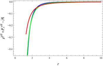
Figure 1: Plots of NEC versus $r$ for $n=1$ (blue), $0.5$ (red) and $-0.5$ (green).

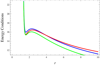
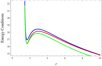
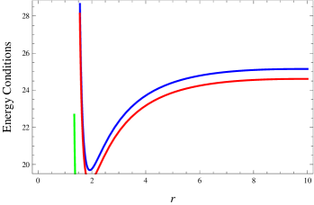
Figure 2: Plots of $\rho-\mathcal{A}$ (blue), $\rho+P_{r}-\mathcal{A}$ (red) and $\rho+P_{t}-\mathcal{A}$ (green) versus $r$ with $\Upsilon=0.05,~{}\mu=1,~{}\nu=-1,~{}a=0.2$ and $b=0.25$. The upper case for $n=1$ (left) and $n=0.5$ (right) while lower case for $n=-0.5$.

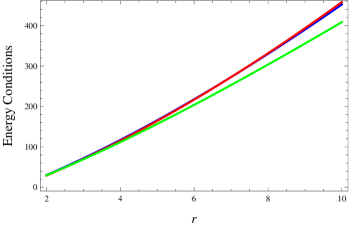
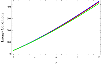
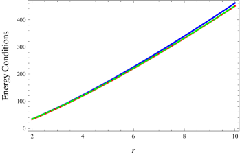
Figure 3: Plots of $\rho-\mathcal{A}$ (blue), $\rho+P_{r}-\mathcal{A}$ (red) and $\rho+P_{t}-\mathcal{A}$ (green) versus $r$ with $\Upsilon=0.05,~{}\mu=-1,~{}\nu=1,~{}a=0.2$ and $b=-0.25$. The upper case for $n=1$ (left) and $n=0.5$ (right) while lower case for $n=-0.5$.

The third possibility to avoid the finite-time future singularities is generally described by $a<0,~{}b>0$ and $b\neq 1$ while the constraint $a+b<1/2$ with $\mu\nu<0$ is also imposed on model parameters. In this case, we arbitrarily choose the values $\mu=-1,~{}\nu=1,~{}a=-0.01$ and $b=0.25$ to analyze the validity of energy conditions given in Figure 4. It is observed that the realistic WH solutions exist in the regions $3.2\leq r\leq 10,~{}3.5\leq r\leq 10$ and $4\leq r\leq 10$ for $n=1,~{}0.5$ and $-0.5$, respectively. Thus, the physically acceptable region decreases as the value of $n$ decreases. Figure 5 shows that NEC as well as WEC remain positive in the region $4\leq r\leq 10$ with the choice of model parameters $a<0,~{}b<0$ and $\mu<0$ particularly for $\mu=-1,~{}\nu=1,~{}a=-0.01$ and $b=-0.25$. In this case, WH geometries are also sustained by normal matter.

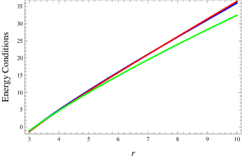
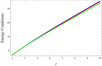
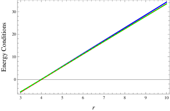
Figure 4: Plots of $\rho-\mathcal{A}$ (blue), $\rho+P_{r}-\mathcal{A}$ (red) and $\rho+P_{t}-\mathcal{A}$ (green) versus $r$ with $\Upsilon=0.05,~{}\mu=-1,~{}\nu=1,~{}a=-0.01$ and $b=0.25$. The upper case for $n=1$ (left) and $n=0.5$ (right) while lower case for $n=-0.5$.

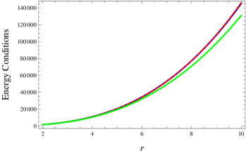
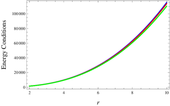
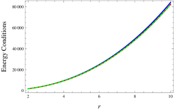
Figure 5: Plots of $\rho-\mathcal{A}$ (blue), $\rho+P_{r}-\mathcal{A}$ (red) and $\rho+P_{t}-\mathcal{A}$ (green) versus $r$ with $\Upsilon=0.05,~{}\mu=-1,~{}\nu=1,~{}a=-0.01$ and $b=-0.25$. The upper case for $n=1$ (left) and $n=0.5$ (right) while lower case for $n=-0.5$.

3.2 Isotropic Fluid

For isotropic matter configuration $P=P_{r}=P_{t}$, Eqs.(11) and (12) lead to

$$[\Upsilon(1-\Upsilon)+(1+\Upsilon)(2+3\Upsilon)]\left[\frac{2\lambda}{r^{3}}\left(1-\frac{\chi}{r}\right)-\frac{\chi}{r^{3}}+\frac{1}{2}\mu\mathcal{G}^{a}(1+\nu\mathcal{G}^{b})\right.$$

$$- \left.\frac{1}{2}\mu\mathcal{G}^{a}[a+\nu(a+b)\mathcal{G}^{b}]-\frac{4\mu\lambda}{r^{5}}(3\chi-2r)\left(1-\frac{\chi}{r}\right)\left\{a(a-1)+\nu(a+b)\right.\right.$$

$$\times \left.\left.(a+b-1)\mathcal{G}^{b}\right\}\mathcal{G}^{a-2}\mathcal{G}^{\prime}\right]+2[(1-\Upsilon)^{2}-\Upsilon(1+\Upsilon)]\left[\frac{\lambda}{r^{4}}(\lambda-r)\left(1-\frac{\chi}{r}\right)\right.$$

$$+ \left.\frac{1}{2r^{4}}(r+\lambda)(\chi-r\chi^{\prime})+\frac{1}{2}\mu\mathcal{G}^{a}(1+\nu\mathcal{G}^{b})-\frac{1}{2}\mu\mathcal{G}^{a}[a+\nu(a+b)\mathcal{G}^{b}]\right.$$

$$+ \left.\frac{2\lambda\mu}{r^{5}}\left(1-\frac{\chi}{r}\right)\left\{2(\lambda-2r)\left(1-\frac{\chi}{r}\right)-3(r\chi^{\prime}-\chi)\right\}\left[a(a-1)+\nu(a+b)\right.\right.$$

$$\times \left.\left.(a+b-1)\mathcal{G}^{b}\right]\mathcal{G}^{a-2}\mathcal{G}^{\prime}+\frac{4\lambda}{r^{3}}\left(1-\frac{\chi}{r}\right)^{2}\left\{a\mu(a-1)\mathcal{G}^{a-2}\left(\mathcal{G}^{\prime\prime}+(a-2)\right.\right.\right.$$

$$\times \left.\left.\left.\frac{\mathcal{G}^{\prime 2}}{\mathcal{G}}\right)+\mu\nu(a+b)(a+b-1)\mathcal{G}^{a+b-2}\left(\mathcal{G}^{\prime\prime}+(a+b-2)\frac{\mathcal{G}^{\prime 2}}{\mathcal{G}}\right)\right\}\right]=0,$$

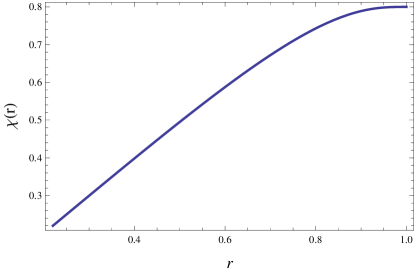
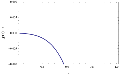
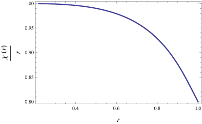
Figure 6: Plots of $\chi(r),~{}\chi(r)-r,~{}\frac{\chi(r)}{r}$ and $\chi^{\prime}(r)$ versus $r$ for $\mu=1,~{}\nu=-1,\newline a=0.2,~{}b=0.25,~{}\lambda=0.01$ and $\Upsilon=0.05$.

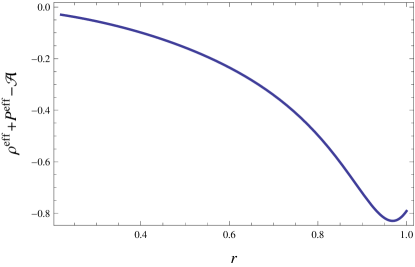
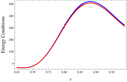
Figure 7: Plots of energy conditions for same values.

where the value of $\mathcal{G}$ is given in Eq.(18). This differential equation is highly non-linear in $\chi(r)$ which cannot be solved analytically. To find its solution, we use the numerical technique and display the corresponding results in Figure 6. The graphical behavior of $\chi(r)$ is given in the upper left panel which shows that the positivity of $\left(1-\frac{\chi}{r}\right)$ is fulfilled throughout the evolution. The right panel indicates that the WH throat is located approximately at $r_{\mathrm{th}}=0.2239$ for which $\chi(r)-r$ approaches to zero but fails to cross the radial axis to get the exact value of $r_{\mathrm{th}}$. The asymptotically flatness condition is not satisfied as given in the lower left case while the right plot shows that the condition $\chi^{\prime}(r_{\mathrm{th}})<1$ is obeyed. In Figure 7 (left), the violating behavior of effective NEC indicates that $f(\mathcal{G},T)$ gravity provides $T_{\alpha\beta}^{\mathrm{eff}}$ as a required alternative source while the right panel shows the plots of $\rho-\mathcal{A}$ (blue) and $\rho+P-\mathcal{A}$ (red). It is observed that both NEC as well as WEC are positive in the region $0.715\leq r<1$ and hence realistic traversable tiny WH can be formed for isotropic fluid.

3.3 Barotropic Fluid

In this case, we explore the WH geometries using barotropic equation of state for both radial as well as tangential pressures. For radial pressure, we take $P_{r}=w\rho$ ($w$ is an equation of state parameter), Eqs.(10) and (11) give

$$[2w+(1+5w)\Upsilon]\left[\frac{\chi^{\prime}}{r^{2}}-\frac{1}{2}\mu\mathcal{G}^{a}(1+\nu\mathcal{G}^{b})+\frac{1}{2}\mu\mathcal{G}^{a}[a+\mu(a+b)\mathcal{G}^{b}]\right.$$ (29)

$$+ \left.\frac{2\mu}{r^{4}}(r\chi^{\prime}-\chi)\left(2-\frac{3\chi}{r}\right)\left[a(a-1)+\nu(a+b)(a+b-1)\mathcal{G}^{b}\right]\mathcal{G}^{a-2}\mathcal{G}^{\prime}\right.$$

$$+ \left.\frac{4\chi}{r^{3}}\left(1-\frac{\chi}{r}\right)\left[a\mu(a-1)\mathcal{G}^{a-2}\left\{\mathcal{G}^{\prime\prime}+(a-2)\frac{\mathcal{G}^{\prime 2}}{\mathcal{G}}\right\}+\mu\nu(a+b)(a+b-1)\right.\right.$$

$$\times \left.\left.\mathcal{G}^{a+b-2}\left\{\mathcal{G}^{\prime\prime}+(a+b-2)\frac{\mathcal{G}^{\prime 2}}{\mathcal{G}}\right\}\right]\right]-[2-(w-3)\Upsilon]\left[\frac{2\lambda}{r^{3}}\left(1-\frac{\chi}{r}\right)-\frac{\chi}{r^{3}}\right.$$

$$+ \left.\frac{1}{2}\mu\mathcal{G}^{a}(1+\nu\mathcal{G}^{b})-\frac{1}{2}\mu\mathcal{G}^{a}[a+\nu(a+b)\mathcal{G}^{b}]-\frac{4\mu\lambda}{r^{5}}(3\chi-2r)\left(1-\frac{\chi}{r}\right)\right.$$

$$\times \left.\left\{a(a-1)+\nu(a+b)(a+b-1)\mathcal{G}^{b}\right\}\mathcal{G}^{a-2}\mathcal{G}^{\prime}\right]+2\Upsilon(1+w)\left[\frac{\lambda}{r^{4}}(\lambda-r)\right.$$

$$\times \left.\left(1-\frac{\chi}{r}\right)+\frac{1}{2r^{4}}(r+\lambda)(\chi-r\chi^{\prime})+\frac{1}{2}\mu\mathcal{G}^{a}(1+\nu\mathcal{G}^{b})-\frac{1}{2}\mu\mathcal{G}^{a}[a+\nu(a+b)\right.$$

$$\times \left.\mathcal{G}^{b}]+\frac{2\lambda\mu}{r^{5}}\left(1-\frac{\chi}{r}\right)\left\{2(\lambda-2r)\left(1-\frac{\chi}{r}\right)-3(r\chi^{\prime}-\chi)\right\}\left[a(a-1)\right.\right.$$

$$+ \left.\left.\nu(a+b)(a+b-1)\mathcal{G}^{b}\right]\mathcal{G}^{a-2}\mathcal{G}^{\prime}+\frac{4\lambda}{r^{3}}\left(1-\frac{\chi}{r}\right)^{2}\left\{a\mu(a-1)\mathcal{G}^{a-2}\right.\right.$$

$$\times \left.\left.\left(\mathcal{G}^{\prime\prime}+(a-2)\frac{\mathcal{G}^{\prime 2}}{\mathcal{G}}\right)+\mu\nu(a+b)(a+b-1)\mathcal{G}^{a+b-2}\right.\right.$$

$$\times \left.\left.\left(\mathcal{G}^{\prime\prime}+(a+b-2)\frac{\mathcal{G}^{\prime 2}}{\mathcal{G}}\right)\right\}\right]=0,$$

which we solve numerically for $\chi(r)$ and present the results in Figure 8. The positively increasing evolution of $\chi(r)$ is shown in the upper left case while the right plot gives the value of WH throat radius. In this case, the throat is located at $r_{\mathrm{th}}=0.1572$ such that $\chi(r_{\mathrm{th}})=r_{\mathrm{th}}$. The lower panel (left) indicates non-asymptotically flat behavior of $\chi(r)$ whereas the constraint $\chi^{\prime}(r)<1$ is satisfied at $r=r_{\mathrm{th}}$ (right). The left plot of Figure 9 indicates negativity of NEC for $T_{\alpha\beta}^{\mathrm{eff}}$ while the right panel shows that NEC as well as WEC for ordinary matter distribution described by $\rho-\mathcal{A}\geq 0$ (blue), $\rho+P_{r}-\mathcal{A}\geq 0$ (red) and $\rho+P_{t}-\mathcal{A}\geq 0$ (green) are satisfied in the region $0.66\leq r\leq 0.90$. Thus, the WH geometries are supported by ordinary matter in this case.

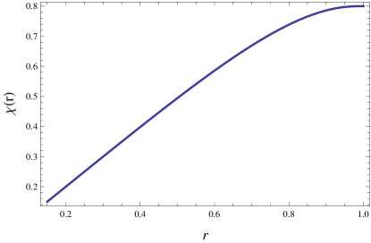
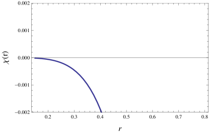
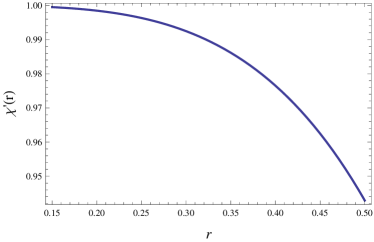
Figure 8: Plots of $\chi(r),~{}\chi(r)-r,~{}\frac{\chi(r)}{r}$ and $\chi^{\prime}(r)$ versus $r$ for $w=-0.1$.

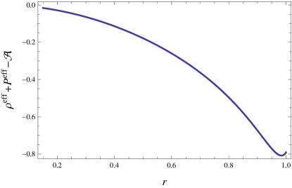
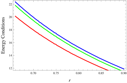
Figure 9: Plots of energy conditions for same values.

In case of tangential pressure, we consider the barotropic equation of state of the form $P_{t}=w\rho$. To analyze the possible existence of WH solutions, Eqs.(10) and (12) give third order differential equation in $\chi(r)$ as

$$(1+\Upsilon)[2w+(1+5w)\Upsilon]\left[\frac{\chi^{\prime}}{r^{2}}-\frac{1}{2}\mu\mathcal{G}^{a}(1+\nu\mathcal{G}^{b})+\frac{1}{2}\mu\mathcal{G}^{a}[a+\mu(a+b)\right.$$ (30)

$$\times \left.\mathcal{G}^{b}]+\frac{2\mu}{r^{4}}(r\chi^{\prime}-\chi)\left(2-\frac{3\chi}{r}\right)\left[a(a-1)+\nu(a+b)(a+b-1)\mathcal{G}^{b}\right]\right.$$

$$\times \left.\mathcal{G}^{a-2}\mathcal{G}^{\prime}+\frac{4\chi}{r^{3}}\left(1-\frac{\chi}{r}\right)\left[a\mu(a-1)\mathcal{G}^{a-2}\left\{\mathcal{G}^{\prime\prime}+(a-2)\frac{\mathcal{G}^{\prime 2}}{\mathcal{G}}\right\}\right.\right.$$

$$+ \left.\left.\mu\nu(a+b)(a+b-1)\mathcal{G}^{a+b-2}\left\{\mathcal{G}^{\prime\prime}+(a+b-2)\frac{\mathcal{G}^{\prime 2}}{\mathcal{G}}\right\}\right]\right]+\Upsilon[(1+w)$$

$$- (1-w)\Upsilon]\left[\frac{2\lambda}{r^{3}}\left(1-\frac{\chi}{r}\right)-\frac{\chi}{r^{3}}+\frac{1}{2}\mu\mathcal{G}^{a}(1+\nu\mathcal{G}^{b})-\frac{1}{2}\mu\mathcal{G}^{a}[a+\nu(a+b)\right.$$

$$\times \left.\mathcal{G}^{b}]-\frac{4\mu\lambda}{r^{5}}(3\chi-2r)\left(1-\frac{\chi}{r}\right)\left\{a(a-1)+\nu(a+b)(a+b-1)\mathcal{G}^{b}\right\}\right.$$

$$\times \left.\mathcal{G}^{a-2}\mathcal{G}^{\prime}\right]+2[w\Upsilon(1+\Upsilon)+(1-\Upsilon)^{2}]\left[\frac{\lambda}{r^{4}}(\lambda-r)\left(1-\frac{\chi}{r}\right)+\frac{1}{2r^{4}}(r+\lambda)\right.$$

$$\times \left.(\chi-r\chi^{\prime})+\frac{1}{2}\mu\mathcal{G}^{a}(1+\nu\mathcal{G}^{b})-\frac{1}{2}\mu\mathcal{G}^{a}[a+\nu(a+b)\mathcal{G}^{b}]+\frac{2\lambda\mu}{r^{5}}\left(1-\frac{\chi}{r}\right)\right.$$

$$\times \left.\left\{2(\lambda-2r)\left(1-\frac{\chi}{r}\right)-3(r\chi^{\prime}-\chi)\right\}\left[a(a-1)+\nu(a+b)(a+b-1)\mathcal{G}^{b}\right]\right.$$

$$\times \left.\mathcal{G}^{a-2}\mathcal{G}^{\prime}+\frac{4\lambda}{r^{3}}\left(1-\frac{\chi}{r}\right)^{2}\left\{a\mu(a-1)\mathcal{G}^{a-2}\left(\mathcal{G}^{\prime\prime}+(a-2)\frac{\mathcal{G}^{\prime 2}}{\mathcal{G}}\right)\right.\right.$$

$$+ \left.\left.\mu\nu(a+b)(a+b-1)\mathcal{G}^{a+b-2}\left(\mathcal{G}^{\prime\prime}+(a+b-2)\frac{\mathcal{G}^{\prime 2}}{\mathcal{G}}\right)\right\}\right]=0.$$

We solve this equation numerically and corresponding results are displayed in Figure 10. Similar behavior of $\chi(r),~{}\frac{\chi(r)}{r}$ and $\chi^{\prime}(r)$ are obtained as in the previous cases. The throat is located at $r_{\mathrm{th}}=0.1585$ where the curve $\chi(r)-r$ approaches to zero. The left panel of Figure 11 shows the violation of NEC in $f(\mathcal{G},T)$ gravity throughout the evolution. The graphs of $\rho-\mathcal{A}\geq 0$ (blue), $\rho+P_{r}-\mathcal{A}\geq 0$ (red) and $\rho+P_{t}-\mathcal{A}\geq 0$ (green) exhibit positive values in the interval $0.66\leq r\leq 0.90$ as shown in Figure 11 (right). Thus, a micro WH can be formed in this physically acceptable region.

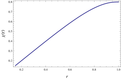
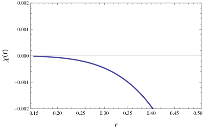
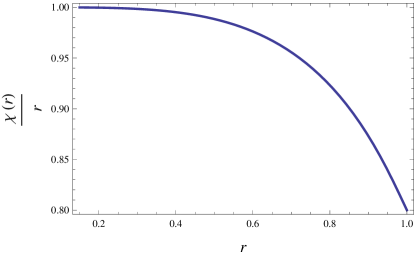
Figure 10: Plots of $\chi(r),~{}\chi(r)-r,~{}\frac{\chi(r)}{r}$ and $\chi^{\prime}(r)$ versus $r$ for $w=-0.04$.

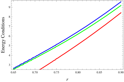
Figure 11: Plots of energy conditions for same values.

4 Final Remarks

In this paper, we have analyzed static spherically symmetric traversable WH solutions in $f(\mathcal{G},T)$ gravity using anisotropic, isotropic as well as barotropic matter distributions. For this purpose, we have considered a particular model $f(\mathcal{G},T)=F(\mathcal{G})+\mathcal{F}(T)$ with specific form of $\psi(r)$ satisfying the no-horizon condition. In $f(\mathcal{G},T)$ gravity, test particles follow non-geodesic trajectories due to the presence of extra force which appears as a consequence of non-zero divergence of the energy-momentum tensor [4]. For the non-geodesic congruences, the divergence of four-acceleration appears in the evolution of expansion scalar [19]. Consequently, the four fundamental energy conditions for non-geodesic congruences are also affected due to the presence of this auxiliary term. We have formulated these non-geodesic energy constraints to explore the existence of realistic WH solutions in this gravity.

For anisotropic fluid, we have considered viable form of $\chi(r)$ which meets all necessary conditions of traversable WH geometry and analyzed the behavior of energy conditions. This analysis is carried out for four possible choices of $F(\mathcal{G})$ model parameters such that they avoid all four types of finite-time future singularities. For isotropic and barotropic (satisfied by radial as well as tangential pressures) matter distributions, we have solved the corresponding differential equations numerically to examine the behavior of $\chi(r)$. The non-asymptotically flat shape functions satisfying the basic requirements for WH geometry are obtained in each case. The violation of NEC defined in $f(\mathcal{G},T)$ gravity is observed throughout the evolution for all three types of matter distribution. This violation confirms the traversability of WH solutions while the positivity of NEC as well as WEC for ordinary matter contents assure the existence of physical acceptable WH geometries in certain regions.

In $f(\mathcal{G})$ gravity, we have found that realistic WH solutions exist only for barotropic fluid satisfied by radial pressure [15]. This difference may be due to the curvature-matter coupling present in $f(\mathcal{G},T)$ gravity. We can conclude that this curvature-matter coupled theory provides an alternative source for the existence of realistic WH solutions.

References

- [1] Deruelle, N.: Nucl. Phys. B 327(1989)253; Deruelle, N. and Faria-Busto, L.: Phys. Rev. D 41(1990)3696; Deruelle, N. and Doleel, T.: Phys. Rev. D 62(2000)103502; Calcagni, G., Tsujikawa, S. and Sami, M.: Class. Quantum Grav. 22(2005)3977; De Felice, A., Hindmarsh, M. and Trodden, M.: J. Cosmol. Astropart. Phys. 08(2006)005.
- [2] Nojiri, S. and Odintsov, S.D.: Phys. Lett. B 631(2005)1.
- [3] Cognola, G. et al.: Phys. Rev. D 73(2006)084007; De Felice, A. and Tsujikawa, S.: Phys. Lett. B 675(2009)1; Phys. Rev. D 80(2009)063516.
- [4] Sharif, M. and Ikram, A.: Eur. Phys. J. C 76(2016)640.
- [5] Sharif, M. and Ikram, A.: Phys. Dark Universe (to appear, 2017), arXiv:1612.02037.
- [6] Einstein, A. and Rosen, N.: Phys. Rev. 48(1935)73.
- [7] Morris, M.S. and Thorne, K.S.: Am. J. Phys. 56(1988)395.
- [8] Bhawal, B. and Kar, S.: Phys. Rev. D 46(1992)2464; Wang, A. and Letelier, P.S.: Prog. Theor. Phys. 94(1995)137; Bronnikov, K.A. and Kim, S.W.: Phys. Rev. D 67(2003)064027; Lobo, F.S.N.: Phys. Rev. D 73(2006)064028; Rahaman, F. et al.: Phys. Rev. D 86(2012)106010; Sharif, M. and Rani, S.: Gen. Relativ. Gravit. 45(2013)2389.
- [9] Furey, N. and DeBenedictis, A.: Class. Quantum Grav. 22(2005)313.
- [10] Lobo, F.S.N. and Oliveira, M.A.: Phys. Rev. D 80(2009)104012.
- [11] Azizi, T.: Int. J. Theor. Phys. 52(2013)3486.
- [12] Sharif, M. and Zahra, Z.: Astrophys. Space Sci. 348(2013)275.
- [13] Sharif, M. and Rani, S.: Adv. High Energy Phys. 2014(2014)691497.
- [14] Mehdizadeh, M.R., Zangeneh, M.K. and Lobo, F.S.N.: Phys. Rev. D 91(2015)084004.
- [15] Sharif, M. and Ikram, A.: Int. J. Mod. Phys. D 24(2015)1550003.
- [16] Zubair, M., Waheed, S. and Ahmad, Y.: Eur. Phys. J. C 76(2016)444.
- [17] Landau, L.D. and Lifshitz, E.M.: The Classical Theory of Fields (Pergamon Press, 1971).
- [18] Poisson, P.: A Relativist’s Toolkit: The Mathematics of Black-Hole Mechanics (Cambridge University Press, 2004).
- [19] Dadhich, N.: arXiv:gr-qc/0511123v2; Kar, S. and Sengupta, S.: Pramana J. Phys. 69(2007)49.
- [20] Kar, S. and Sahdev, D.: Phys. Rev. D 52(1995)2030.
- [21] Bamba, K. et al.: Eur. Phys. J. C 67(2010)295.
- [22] Pavlovic, P. and Sossich, M.: Eur. Phys. J. C 75(2015)117.