Deviations from Wick’s theorem in the canonical ensemble

Abstract

Wick’s theorem for the expectation values of products of field operators for a system of noninteracting fermions or bosons plays an important role in the perturbative approach to the quantum many body problem. A finite temperature version holds in the framework of the grand canonical ensemble but not for the canonical ensemble appropriate for systems with fixed particle number like ultracold quantum gases in optical lattices. Here we present new formulas for expectation values of products of field operators in the canonical ensemble using a method in the spirit of Gaudin’s proof of Wick’s theorem for the grand canonical case. The deviations from Wick’s theorem are examined quantitatively for two simple models of noninteracting fermions.

I Introduction

Properties of a large system of noninteracting fermions or bosons in thermal equilibrium are usually described using the grand canonical ensemble with variable particle number. For a system of fixed number $N$ of fermions in a closed box this provides an excellent approximation for large enough $N$. An exception is provided by the ideal Bose gas, where the probability distribution for the particle number in the lowest one-particle state fails badly in the low temperature limit as the comparison for the appropriate result within the canonical ensemble shows Mullin ; Scully .

In a recent publication a new formula for the $n$-particle density matrices in the canonical ensemble was presented KTTK . In contrast to Wick’s theorem for the grand canonical ensemble the higher order reduced density matrices cannot be expressed in terms of the one-particle function. Here a different approach in the spirit of Gaudin’s proof of Wick’s theorem for the grand canonical ensemble Gaudin ; FW is presented.

In section II earlier results for expectation values of occupation numbers and products of them are discussed. In contrast to the grand canonical ensemble no simple factorization of the expectation values of products of occupation number operators occurs when the canonical ensemble is used. The formulas presented earlier involve a summation which involves all partition functions for particle number from one to $N$, which are numerically rather unstable for large values of $N$.

In section III new formulas are derived in which expectation values of $m$-particle operators are expressed in terms of the mean occupation numbers. For simple models like one-dimensional fermions in a harmonic trap and a zero bandwidth semiconductor explicit results are presented and the deviations from Wick’s theorem are elucidated quantitatively in section IV. Analytical expressions for the deviation from Wick’s theorem are presented.

II Known results for noninteracting fermions in the canonical and grand canonical ensemble

An $N$-particle system with Hamiltonian $H_{N}$ in thermal equilibrium at temperature $T$ is described by the canonical statistical operator

$$\rho_{c}=e^{-\beta H_{N}}/Z_{N}~{},~{}~{}~{}~{}Z_{N}=Tr_{N}e^{-\beta H_{N}}~{},$$ (1)

where $\beta=1/(k_{B}T)$ with $k_{B}$ Boltzmann’s constant and $Tr_{N}$ the trace over the $N$-particle Hilbert space. The expectation value of an observable $A$ is given by

$$\langle A\rangle_{c}=Tr_{N}Ae^{-\beta H_{N}}/Z_{N}~{}.$$ (2)

In this paper systems of $N$ noninteracting fermions with $H_{N}=\sum_{\alpha=1}^{N}h_{\alpha}$ are considered. The eigenstates of such a system can be expressed as a determinant of the single particle eigenstates obeying the single particle Schrödinger equation $h|\epsilon_{i}\rangle=\epsilon_{i}|\epsilon_{i}\rangle$. A convenient way to express the $N$-particle eigenstates is by the list of occupation numbers $\{n\}$ of these one-particle states leading to

$$H_{N}|\{n\}\rangle_{N}=\sum_{i}\epsilon_{i}n_{i}|\{n\}\rangle_{N}$$ (3)

with $\sum_{i}n_{i}=N$. For fermions the occupation numbers $n_{i}$ can take the values $0$ and $1$. The canonical partition function is given by

$$Z_{N}(\beta)=\sum_{\{n\}}e^{-\beta\sum_{j}\epsilon_{j}n_{j}}\delta_{N,\sum_{j}n_{j}}$$ (4)

The Kronecker delta restricting the occupation number sums makes a closed evaluation of $Z_{N}$ generally difficult. Therefore for large particle number $N$ the grand canonical statistical operator $\rho_{gc}$ with varying particle number is often used. It acts in Fock space which is the direct sum over all $N$ from zero to infinity of the Hilbert spaces of totally antisymmetric $N$-particle states. In this context it is appropriate to use second quantization by introducing the creation and annihilation operators $c^{\dagger}_{i}$ and $c_{i}$ of the orthonormal one-particle state $|i\rangle$ obeying the anticommutation rules $[c_{i},c_{j}]_{+}=0$ and $[c_{i},c^{\dagger}_{j}]_{+}=\delta_{ij}$. For the noninteracting systems treated in this paper the Hamiltonian $H_{0}$ reads

$$H_{0}=\sum_{i}\epsilon_{i}c^{\dagger}_{i}c_{i}=\sum_{i}\epsilon_{i}n_{i}$$ (5)

if $c^{\dagger}_{i}$ creates a fermion in the energy eigenstate $|\epsilon_{i}\rangle$. The $n_{i}=c^{\dagger}_{i}c_{i}$ are the occupation number operators. The corresponding grand canonical statistical operator reads

$$\rho_{gc}^{(0)}=e^{-\beta\tilde{H}_{0}}/Z_{F}~{},~{}~{}~{}~{}Z_{F}=Tr_{F}e^{-\beta\tilde{H}_{0}}~{},$$ (6)

where $\tilde{H}_{0}\equiv H_{0}-\mu{\cal N}$ with ${\cal N}=\sum_{i}n_{i}$ the particle number operator expressed in terms of the occupation number operators and $\mu$ the chemical potential. Because it simplifies the calculations the grand canonical ensemble is often used as an approximate description for a system with fixed particle number $N$, using $\langle{\cal N}\rangle_{gc}=N$ to fix the chemical potential.

In the rest of this section we discuss known results for the expectation values $\langle n_{i}\rangle$ and $\langle n_{i}n_{j}\rangle$ with $i\neq j$ for both ensembles. We begin with the much simpler case of the grand canonical ensemble. The statistical operator $\rho_{gc}^{(0)}$ factorizes

$$\rho_{gc}^{(0)}=\prod_{i}e^{-\beta\tilde{\epsilon}_{i}n_{i}}/z_{i}\equiv\prod_{i}\rho_{i}^{(0)}$$ (7)

with $\tilde{\epsilon}_{i}=\epsilon_{i}-\mu$ and $z_{i}=1+e^{-\beta\tilde{\epsilon}_{i}}$. This leads to $\langle n_{i}\rangle_{gc}=e^{-\beta\tilde{\epsilon}_{i}}/z_{i}$ and one obtains the Fermi function

$$\langle n_{i}\rangle_{gc}=\frac{1}{e^{\beta\tilde{\epsilon}_{i}}+1}\equiv f(\tilde{\epsilon}_{i})~{}.$$ (8)

Because of the factorization of $\rho_{gc}^{(0)}$ the factorization for the expectation value of two different occupation number operators easily follows

$$\langle n_{i}n_{j}\rangle_{gc}=\langle n_{i}\rangle_{gc}\langle n_{j}\rangle_{gc}~{}.$$ (9)

This is the simplest version of Wick’s theorem. The total factorization of a product of an arbitrary number of different occupation number operators is obvious. It is discussed in more detail in the next section.

With Eqs. (8) and (9) a simple expression for the mean square deviation of the total particle number can be given. With $n_{i}^{2}=n_{i}$ one obtains

$$\langle{\cal N}^{2}\rangle_{gc} = \sum_{i\neq j}\langle n_{i}n_{j}\rangle_{gc}+\sum_{i}\langle n_{i}\rangle_{gc}$$

$$= \sum_{i\neq j}\langle n_{i}\rangle_{gc}\langle n_{j}\rangle_{gc}+\sum_{i}\langle n_{i}\rangle_{gc}$$

leading to

$$\langle{\cal N}^{2}\rangle_{gc}-\langle{\cal N}\rangle_{gc}^{2}=\sum_{i}\langle n_{i}\rangle_{gc}(1-\langle n_{i}\rangle_{gc})~{}.$$ (11)

As the right hand side of this equation is of order $N$ (see section III for explicit examples), the relative width of the particle number distribution in the grand canonical ensemble decreases like $1/\sqrt{N}$ in the large $N$ limit.

For the canonical ensemble the mean occupation numbers $\langle n_{i}\rangle_{N}$

$$\langle n_{i}\rangle_{N,c}=\frac{1}{Z_{N}}\sum_{\{n\}}n_{i}e^{-\beta\sum_{j}\epsilon_{i}n_{j}}\delta_{N,\sum_{j}n_{j}}$$ (12)

were early studied by Schmidt Schmidt . He derived a simple relation between $\langle n_{i}\rangle_{N}$ and $\langle n_{i}\rangle_{N-1}$ (we suppress the index “$c$” for the rest of this section)

$$\langle n_{i}\rangle_{N}=e^{-\beta\epsilon_{i}}\frac{Z_{N-1}}{Z_{N}}(1-\langle n_{i}\rangle_{N-1})$$ (13)

by performing the $n_{i}$ sum and introducing the factor $1-n_{i}$ in order to return to the complete sum over $\{n\}$ with $N$ replaced by $N-1$ in the Kronecker delta. In the large $N$ limit $\langle n_{i}\rangle_{N}\approx\langle n_{i}\rangle_{N-1}$ and $Z_{N-1}/Z_{N}=e^{\beta(F_{N}-F_{N-1})}\approx e^{\beta\mu}$ with $F_{N}$ the free energy and $\mu$ the chemical potential holds, leading to the Fermi function

$$\langle n_{i}\rangle_{N}\approx(e^{\beta(\epsilon_{i}-\mu)}+1)^{-1}=f(\tilde{\epsilon}_{i})~{}.$$ (14)

For arbitrary values of $N$ the recursion relation in Eq.(13) can be used. With the initial value $\langle n_{i}\rangle_{0}=0$ one obtains in the first step $\langle n_{i}\rangle_{1}=e^{-\beta\epsilon_{i}}/Z_{N}$ and easily proves by induction

$$\langle n_{i}\rangle_{N}=\frac{1}{Z_{N}}\sum_{k=1}^{N}(-1)^{k-1}e^{-\beta k\epsilon_{i}}Z_{N-k}(\beta)~{}.$$ (15)

The summation over all $i$ yields $N$ on the left hand side leading to

$$Z_{N}(\beta)=\frac{1}{N}\sum_{k=1}^{N}(-1)^{k-1}Z_{N-k}(\beta)Z_{1}(k\beta)$$ (16)

with $Z_{1}(\beta)=\sum_{i}e^{-\beta\epsilon_{i}}$. There are also other ways to derive this relation BF1 . The sums in Eqs. (15) and (16) unfortunately are numerically rather unstable for large values of $N$. BF2 They also do not provide analytical expressions in the limiting cases discussed in section IV.

The procedure leading to Eq.(13) can easily be extended to the calculation of expectation values of products of different occupation numbers. Replacing $n_{i}$ by $n_{i}n_{j}$ in Eq. (12) with $i\neq j$ one obtains

$$\langle n_{i}n_{j}\rangle_{N}=\frac{Z_{N-2}}{Z_{N}}e^{-\beta(\epsilon_{i}+\epsilon_{j})}\langle(1-n_{i})(1-n_{j})\rangle_{N-2}~{}.$$ (17)

The large $N$ limit can be treated as following Eq. (13). With the additional assumption $\langle n_{i}n_{j}\rangle_{N}\approx\langle n_{i}n_{j}\rangle_{N-2}$ one obtains using Eq. (14) after elementary algebra

$$\langle n_{i}n_{j}\rangle_{N}\approx[(e^{\beta(\epsilon_{i}-\mu)}+1)(e^{\beta(\epsilon_{j}-\mu)}+1)]^{-1}$$ (18)

i.e. the simplest version of Wick’s theorem $\langle n_{i}n_{j}\rangle=\langle n_{i}\rangle\langle n_{j}\rangle$ approximately holds for large $N$ also in the canonical ensemble. For arbitrary values of $N$ one again can proceed recursively. With the starting value $\langle n_{i}n_{j}\rangle_{2}=e^{-\beta(\epsilon_{i}+\epsilon_{j})}/Z_{2}$ one can show by induction

$$\langle n_{i}n_{j}\rangle_{N}=\frac{1}{Z_{N}}\sum_{k=2}^{N}(-1)^{k}Z_{N-k}\sum_{l=1}^{k-1}e^{-\beta[k\epsilon_{i}+(k-l)\epsilon_{j}]}~{}.$$ (19)

This equation also readily follows from Eq. (5b) of reference 3. Expectation values of higher products of occupation number operators are discussed with a new approach in the next section.

III Wick’s theorem and weaker forms of it

III.1 General remarks

In this section we address Wick’s theorem and weaker forms of it in a more general setting and consider expectation values of multiple products of creation and annihilation operators. A general $m$-particle operator can be written as a linear combination of such a multiple product of $m$ creation and $m$ annihilation operators FW

$$A_{k_{1}k_{2}...k_{m},l_{1}l_{2}...l_{m}}=c^{\dagger}_{k_{1}}c^{\dagger}_{k_{2}}...c^{\dagger}_{k_{m}}c_{l_{m}}c_{l_{m-1}}...c_{l_{1}}~{}.$$ (20)

For the case of fermions treated here all $k_{i}$ and all $l_{j}$ have to be different in order to obtain a non-zero expression. The two-particle interaction $V$ between fermions is an important $m=2$ example. If it is treated in the Hartree-Fock approximation its expectation value in a system of noninteracting fermions occurs. This is one motivation for the following. In a higher order perturbative treatment of a two-particle interaction expectation values of products of operators $A^{(2)}$ occur which can be reordered into operators of the type in Eq. (20). In the following we want to evaluate the expectation value

$$\langle A_{k_{1}k_{2}...k_{m},l_{1}l_{2}...l_{m}}\rangle={\rm Tr}(A_{k_{1}k_{2}...k_{m},l_{1}l_{2}...l_{m}}\rho)$$ (21)

with $\rho$ being the statistical operator for the canonical or the grand canonical ensemble. Performing the trace in both cases using the occupation number states $|\{n\}\rangle_{N}$ it is obvious that the $\{l_{j}\}$ in Eq. (20) have to be a permutation of the $\{k_{i}\}$ in order to obtain a nonzero expectation value. This implies

$$\langle A_{k_{1}k_{2}...k_{m},l_{1}l_{2}...l_{m}}\rangle=\det(\delta^{(m)})\langle n_{l_{1}}n_{l_{2}}...n_{l_{m}}\rangle$$ (22)

where $\delta^{(m)}$ is the $m\times m$ matrix with matrix elements $\delta^{(m)}_{ij}=\delta_{k_{i}l_{j}}$. This result holds for the canonical and the grand canonical ensemble. For $m=1$ this equation reads $\langle c^{\dagger}_{k}c_{l}\rangle=\delta_{kl}\langle n_{l}\rangle$.

III.2 The grand canonical ensemble

As mentioned in section II the factorization of $\rho_{gc}^{(0)}$ (see Eq.(7)) immediately implies

$$\langle P^{(m)}\rangle_{gc}\equiv\langle n_{l_{1}}...n_{l_{m}}\rangle_{gc}=\langle n_{l_{1}}\rangle_{gc}...\langle n_{l_{m-1}}\rangle_{gc}\langle n_{l_{m}}\rangle_{gc}~{}.$$ (23)

Introducing the matrix $\langle c^{\dagger}c\rangle^{(m)}$ with matrix elements $\langle c^{\dagger}c\rangle^{(m)}_{ij}=\langle c^{\dagger}_{k_{i}}c_{l_{j}}\rangle_{gc}$ the expectation value of $A_{k_{1}k_{2}...k_{m},l_{1}l_{2}...l_{m}}$ can be written in the two forms

$$\langle A_{k_{1}k_{2}...k_{m},l_{1}l_{2}...l_{m}}\rangle_{gc} = \det(\delta^{(m)})\prod_{i=1}^{m}\langle n_{l_{i}}\rangle_{gc}$$ (24)

$$=\det(\langle c^{\dagger}c\rangle^{(m)})~{}.$$

Due the multilinearity of the determinant the second form also holds for arbitrary operators $c_{\alpha}=\sum_{i}\langle\alpha|\epsilon_{i}\rangle c_{i}$ in the definition of $A$. This a general form of Wick’s theorem for fermions.

For the attempt to express $\langle A_{k_{1}k_{2}...k_{m},l_{1}l_{2}...l_{m}}\rangle$ in terms of the mean occupation numbers $\langle n_{i}\rangle$ also for the canonical ensemble it is useful to present an alternative way to calculate expectation values of the type $\langle\tilde{A}c_{i}\rangle_{gc}$, where $\tilde{A}$ is an arbitrary product of $m$ creation and $m-1$ annihilation operators. The essential steps in Gaudin’s method Gaudin ; FW to determine such expectation values for fermions or bosons are to use Heisenberg type operators

$$e^{\beta\tilde{H}_{0}}c_{i}e^{-\beta\tilde{H}_{0}}=e^{-\beta\tilde{\epsilon}_{i}}c_{i}$$ (25)

and the cyclic invariance of the trace. This leads to

$${\rm Tr}_{F}\tilde{A}c_{i}e^{-\beta\tilde{H}_{0}} = {\rm Tr}_{F}\tilde{A}e^{-\beta\tilde{H}_{0}}e^{\beta\tilde{H}_{0}}c_{i}e^{-\beta\tilde{H}_{0}}$$ (26)

$$= e^{-\beta\tilde{\epsilon}_{i}}{\rm Tr}_{F}\tilde{A}e^{-\beta\tilde{H}_{0}}c_{i}$$

$$= e^{-\beta\tilde{\epsilon}_{i}}{\rm Tr}_{F}c_{i}\tilde{A}e^{-\beta\tilde{H}_{0}}~{}.$$

Now one can use $c_{i}\tilde{A}=\mp\tilde{A}c_{i}+[c_{i},\tilde{A}]_{\pm}$, where the upper (lower) sign is for fermions (bosons). Multiplication with $e^{\beta\tilde{\epsilon}_{i}}/Z_{F}$ yields

$$(e^{\beta\tilde{\epsilon}_{i}}\pm 1)\langle\tilde{A}c_{i}\rangle_{gc}=\langle[c_{i},\tilde{A}]_{\pm}\rangle_{gc}~{}.$$ (27)

For $\tilde{A}=c_{j}^{\dagger}$ one obtains the expected result

$$\langle c_{j}^{\dagger}c_{i}\rangle_{gc}=\delta_{ij}\frac{1}{e^{\beta\tilde{\epsilon}_{i}}\pm 1}=\delta_{ij}\langle n_{i}\rangle_{gc}$$ (28)

For the case where $\tilde{A}$ is a product of $m$ creation and $m-1$ annihilation operators we return to the fermionic case with $i\to l_{m}$ and $\tilde{A}=P^{(m-1)}c_{l_{m}}^{\dagger}$ addressed in Eq. (23). As all $l_{i}$ in $P^{(m)}$ differ, $c_{l_{m}}$ commutes with $P^{(m-1)}$ i.e. $[c_{l{m}},P^{(m-1)}c^{\dagger}_{l{m}}]_{+}=P^{(m-1)}$ leading to

$$\langle n_{l_{1}}...n_{l_{m}}\rangle_{gc}=\langle n_{l_{1}}...n_{l_{m-1}}\rangle_{gc}\langle n_{l_{m}}\rangle_{gc}~{}.$$ (29)

Iteration leads to the complete factorization. Despite the fact that the direct derivation of Eq. (23) using the factorization of $\rho_{gc}^{(0)}$ is much simpler, Gaudin’s method was shown, as an extension of it can be used also for the case of the canonical ensemble.

III.3 The canonical ensemble

As Eq. (22) also holds in the canonical ensemble one has again only to address expectation values of products of occupation number operators. In reference 3 a general expression for the expectation value of $m$-particle operators in the position and spin representation was presented. Their Eq. (2) leads for the expectation value of a product of $m$ different occupation number operators to

$$\langle n_{l_{1}}...n_{l_{m}}\rangle_{c}=\sum_{k=m}^{N}(-1)^{k-m}Z_{N-k}~{}s^{(k)}_{l_{1}l_{2}...l_{m}}$$ (30)

with

$$s^{(k)}_{l_{1}l_{2}...l_{m}}=\sum_{j_{1}=1}^{k}\sum_{j_{2}=1}^{k}...\sum_{j_{m}=1}^{k}e^{-\beta\sum_{i=1}^{m}j_{i}\epsilon_{l_{i}}}\delta_{j_{1}+j_{2}+...+j_{m},k}~{}.$$ (31)

This generalizes the expressions for $m=1$ and $m=2$ presented in section II. For the case of bosons the factor $(-1)^{k-m}$ is missing. We return to this expression in appendix A.

In the following we propose a new approach to the calculation of $\langle n_{l_{1}}...n_{l_{m}}\rangle_{c}$ which provides analytical expressions in the limiting cases for the models discussed in section IV.

In the canonical ensemble the cyclic move of $c_{i}$ in the trace in Eq. (26) is not allowed as $c_{l_{m}}|~{}\rangle_{N}$ leaves the Hilbert space with fixed $N$. We therefore have to proceed differently here. We treat expectation values of the type $\langle\bar{A}c_{j}^{\dagger}c_{i}\rangle$, where $j\neq i$ and $\bar{A}$ is an arbitrary product of $m-1$ creation and $m-1$ annihilation operators. The cyclic move of $c_{j}^{\dagger}c_{i}$ in the trace in Eq. (26) is possible in the grand canonical as well as the canonical ensemble. Therefore no index for the expectation values is used in the following. The relation

$$e^{\beta H_{0}}c^{\dagger}_{j}c_{i}e^{-\beta H_{0}}=e^{\beta(\epsilon_{j}-\epsilon_{i})}c^{\dagger}_{j}c_{i}$$ (32)

holds without and with the tilde on $H_{0}$. In order to obtain an equation for $\langle\bar{A}c_{j}^{\dagger}c_{i}\rangle$ we here use $c_{j}^{\dagger}c_{i}\bar{A}=\bar{A}c_{j}^{\dagger}c_{i}+[c_{j}^{\dagger}c_{i},\bar{A}]$, with the commutator for fermions as well as bosons after the cyclic move. This leads to

$$(e^{\beta(\epsilon_{i}-\epsilon_{j})}-1)\langle\bar{A}c_{j}^{\dagger}c_{i}\rangle=\langle[c_{j}^{\dagger}c_{i},\bar{A}]\rangle~{}.$$ (33)

In order to solve this equation for $\langle\bar{A}c_{j}^{\dagger}c_{i}\rangle$ the one-particle energies of the states $j$ and $i$ have to differ. We later discuss this condition in more detail and assume $\epsilon_{i}\neq\epsilon_{j}$ in the following. The choice $\bar{A}=c_{i}^{\dagger}c_{j}$ leads to the simplest nontrivial relation. This gives a formula for $\langle c_{i}^{\dagger}c_{j}c_{j}^{\dagger}c_{i}\rangle=\langle n_{i}(1\mp n_{j})\rangle$. With $[c_{j}^{\dagger}c_{i},c_{i}^{\dagger}c_{j}]=n_{j}-n_{i}$ Eq. (33) leads to

$$\langle c_{i}^{\dagger}c_{j}c_{j}^{\dagger}c_{i}\rangle=\frac{\langle n_{j}\rangle-\langle n_{i}\rangle}{e^{\beta(\epsilon_{i}-\epsilon_{j})}-1}~{},$$ (34)

valid for both ensembles and fermions as well as bosons. A detailed discussion of this result in a slightly modified form will be presented later.

In the following we focus on $\langle P^{(m)}\rangle$ defined in Eq. (23). Only if the spectrum of one-particle energies $\epsilon_{i}$ is non-degenerate a complete treatment is possible as all quantum numbers $l_{i}$ in the product $P^{(m)}$ differ. This is e.g. the case for one-dimensional spinless fermions in an external potential, like a box potential or a harmonic well treated as an example in the next section.

Using the anticommutation rule we rewrite the last two occupation number operators in $P^{(m)}$ in the spirit of the simple example just discussed

$$n_{l_{m-1}}n_{l_{m}}=n_{l_{m-1}}-c^{\dagger}_{l_{m-1}}c_{l_{m}}c^{\dagger}_{l_{m}}c_{l_{m-1}}~{}.$$ (35)

With

$$\bar{A}=P^{(m-2)}c^{\dagger}_{l_{m-1}}c_{l_{m}}$$ (36)

the product of the occupation number operators is given by

$$P^{(m)}=P^{(m-1)}-\bar{A}c^{\dagger}_{l_{m}}c_{l_{m-1}}$$ (37)

The commutator in Eq. (33) is readily evaluated as $c^{\dagger}_{l_{m}}c_{l_{m-1}}$ commutes with $P^{(m-2)}$. With $[c^{\dagger}_{l_{m}}c_{l_{m-1}},c^{\dagger}_{l_{m-1}}c_{l_{m}}]=n_{l_{m}}-n_{l_{m-1}}$ used earlier one obtains

$$\langle[c^{\dagger}_{l_{m}}c_{l_{m-1}},\bar{A}]\rangle=\langle P^{(m-2)}(n_{l_{m}}-n_{l_{m-1}})\rangle~{}.$$ (38)

From Eqs. (37) and (33) one obtains in the non-degenerate case assumed in the following

$$\langle P^{(m)}\rangle=\frac{\langle P^{(m-2)}n_{l_{m-1}}\rangle e^{\beta\epsilon_{l_{m-1}}}-\langle P^{(m-2)}n_{l_{m}}\rangle e^{\beta\epsilon_{l_{m}}}}{e^{\beta\epsilon_{l_{m-1}}}-e^{\beta\epsilon_{l_{m}}}}~{}.$$ (39)

This holds for the canonical as well as the grand canonical averages. For the case of the canonical ensemble this relation could have been found earlier by using Eqs. (30) and (31) (see appendix A).

For $m=2$ this equation reads

$$\langle n_{l_{1}}n_{l_{2}}\rangle=\frac{\langle n_{l_{1}}\rangle e^{\beta\epsilon_{l_{1}}}-\langle n_{l_{2}}\rangle e^{\beta\epsilon_{l_{2}}}}{e^{\beta\epsilon_{l_{1}}}-e^{\beta\epsilon_{l_{2}}}}~{}.$$ (40)

This is a slightly different version of Eq. (34) which holds for fermions as well as bosons. One obtains a minus sign in front of the expression on the rhs of Eq. (40) for the case of bosons.

As a test for the grand canonical ensemble one can put in the Fermi functions for the $\langle n_{l_{i}}\rangle$ and readily sees the factorization which holds in contrast to the canonical ensemble. The deviations from the factorization in this case will be quantitatively studied for simple models in the next section.

With the result for $m=2$ the calculation of $\langle P^{(3)}\rangle$ using Eq. (39) suggests the following general result

$$\langle n_{l_{1}}....n_{l_{m}}\rangle=\sum_{i=1}^{m}\langle n_{l_{i}}\rangle\prod_{j(\neq i)}^{m}\frac{e^{\beta\epsilon_{l_{i}}}}{e^{\beta\epsilon_{l_{i}}}-e^{\beta\epsilon_{l_{j}}}}~{}.$$ (41)

It is obviously fullfilled for $m=2$. If this is inserted on the right hand side of Eq. (39) for the expectation values of $m-1$ occupation number operators, simple algebra presented in Appendix B completes the inductive proof of Eq. (41). Together with Eq. (22) this shows that one can express the expectation value of an arbitrary $m$-particle operator in terms of the expectation values $\langle n_{l_{i}}\rangle$ also within the canonical ensemble. Obviously this new result is more complicated than Wick’s theorem Eq. (23) for the grand canonical average. The complete factorization in this case easily follows from Eq. (41). This is also shown in Appendix B.

From the fact that the use of the Fermi functions in Eq. (41) leads to the factorization of the expectation value one expects that the deviations from Wick’s theorem in the canonical ensemble are large for quantum numbers $l_{i}$ where the $\langle n_{l_{i}}\rangle_{c}$ differ strongly from $\langle n_{l_{i}}\rangle_{gc}$. To test this quantitatively we calculate the “Wick ratio”

$$r_{W}^{l_{1}l_{2}}(T,N)\equiv\frac{\langle n_{l_{1}}n_{l_{2}}\rangle_{c}}{\langle n_{l_{1}}\rangle_{c}\langle n_{l_{2}}\rangle_{c}}$$ (42)

as well as the correspondingly defined Wick ratio for higher products of occupation number operators for special models . The deviation from Wick’s theorem is quantified by how much $r_{W}$ differs from one.

IV Applications

In this section we present quantitative results for the deviation from Wick’s theorem in the canonical ensemble for two rather different models.

Fermions in one dimension in a harmonic potential are an example of a system with an equidistant one-particle spectrum. Such a system can be realized in ultracold gases Jochim . In the non-interacting case exact results for the thermodynamic properties and the mean occupation numbers can be obtained with a recursive method KS1 . Here we use these results for the mean occupation numbers in Eqs. (40) and (41) to calculate expectation values of products of occupation number operators for arbitrarily large numbers $N$ of fermions. This model also plays an important role in the context of the Tomonaga-Luttinger model Haldane .

In order to address the problem of Eqs. (40) and (41) with degeneracies of the one-particle energies a simple “semiconductor model” is studied with zero width of the valence and conduction bands. The particle number $N$ is chosen to be equal to the number of valence band states. For this simple model a direct combinatorical method can be used to calculate the canonical mean occupation numbers. It avoids the numerical problems when using Eq. (15) and easily allows to understand how the grand canonical results arises in the large $N$ limit.

IV.1 Fermions in a one-dimensional harmonic trap

We consider $N$ noninteracting spinless fermions in a system with nondegenerate equidistant one-particle energies $\epsilon_{i}$

$$\epsilon_{i}=i\Delta~{},~{}~{}~{}i=1,2,3,....,\infty~{}.$$ (43)

By performing the sum over $n_{1}$ in Eq. (4) only, as a first step, a recursive approach leads to an explicit analytical expression for $Z_{N}$ KS1 . This canonical partition function has the form as for a system of $N$ uncoupled harmonic oscillators with frequencies $\omega_{m}=m\Delta/\hbar,~{}m=1,...,N$. Proceeding similarly for the mean occupation numbers one obtains the recursion relation KS1

$$\langle n_{i}\rangle_{N}=e^{-\beta N\Delta}\langle n_{i-1}\rangle_{N}+(1-e^{-\beta N\Delta})\langle n_{i-1}\rangle_{N-1}.$$ (44)

Together with the “Schmidt relation” Eq. (13) one can obtain a recursion relation between the mean occupation numbers with the same total particle number only

$$\langle n_{i+1}\rangle_{N}=1-e^{-\beta N\Delta}-(e^{-\beta(N-i)\Delta}-e^{-\beta N\Delta})\langle n_{i}\rangle_{N}~{}.$$ (45)

Using it with $\langle n_{1}\rangle_{N}=1-e^{-\beta N\Delta}$ as the starting point, provides an “upward” way to calculate the $\langle n_{i}\rangle_{N}$. Alternatively one can use Eq. (45) to express $\langle n_{i}\rangle_{N}$ in terms of $\langle n_{i+1}\rangle_{N}$ and start the downward iteration for $m+1\gg N$ with $\langle n_{m+1}\rangle_{N}=0$. Together this provides an efficient numerically stable procedure to calculate the mean occupation numbers. In the general case one has to compare $k_{B}T$ with two energy scales, $\Delta$ and $N\Delta$. In the scaling limit $N\to\infty$ with fixed $\beta\Delta$ the recursion relation Eq. (45) for $\bar{n}_{l}\equiv\langle n_{N+l}\rangle_{N}$ simplifies to

$$\bar{n}_{l+1}=1-q^{-l}\bar{n}_{l}~{},~{}~{}~{}~{}\bar{n}_{l}=q^{l}(1-\bar{n}_{l+1}),$$ (46)

whith $q=e^{-\beta\Delta}$. For $1d$ fermions with a linear dispersion this scaling limit corresponds to the addition of an infinite “Dirac sea”SM . Due to the symmetry relation KS1

$$\bar{n}_{-l}=1-\bar{n}_{l+1}$$ (47)

only the upward or the downward recursion has to be used. As long as $k_{B}T\ll N\Delta$ holds, Eq. (46) provides an excellent approximation for very large but finite $N$. Only how $k_{B}T$ compares to $\Delta$ matters in this limit. For $(N\Delta\gg)k_{B}T\gg\Delta$ the $\bar{n}_{l}$ approach the grand canonical Fermi function $f_{l}=1/(e^{\beta(l-1/2)\Delta}+1)$, while for $k_{B}T\ll\Delta$ there are appreciable deviations KS1 .

After this summary of previous results we address the Wick ratio $r_{W}$ for this model. With the definition $\bar{n}_{l}\equiv\langle n_{N+l}\rangle_{N}$ Eq. (40) reads

$$\langle n_{N+i+l}n_{N+i}\rangle=\frac{\bar{n}_{i+l}-q^{l}\bar{n}_{i}}{1-q^{l}}$$ (48)

For arbitrary values of $i$ and $l$ the expectation value $\langle n_{N+i+l}n_{N+i}\rangle$ follows from the numerical values for the mean occupation numbers. As in the scaling limit $N\to\infty$ various analytical results can be obtained we focuss on this limit where Eq. (46) can be used to obtain the mean occupation numbers.

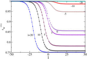
Figure 1: Wick ratio $r_{W}^{i+l,i}$ for $q=e^{-\beta\Delta}=0.75$ as a function of $l(\neq 0)$ for different values of $i$ indicated at the corresponding “curves”. The asymtotic values for large positive and negative values of $l$ are discussed in the text.

In Fig. 1 we present results for the Wick ratio $r_{W}^{i+l,i}=\langle n_{N+i+l}n_{N+i}\rangle/(\bar{n}_{i+l}\bar{n}_{i})$ for $q=0.75$ as a function of $l(\neq 0)$ for different values of $i$. The asymptotic values for $l\to\pm\infty$ can be understood analytically using Eq. (46). For large enough $l$ the second equation implies $\bar{n}_{i+l}\approx q^{i+l}$ and

$$\bar{n}_{i+l}-q^{l}\bar{n}_{i}\approx q^{i+l}(1-q^{-i}\bar{n}_{i})=q^{i+l}\bar{n}_{i+1}\approx\bar{n}_{i+l}\bar{n}_{i+1}~{}.$$ (49)

This implies

$$l\to\infty:~{}~{}r_{W}^{i+l,i}\to\bar{n}_{i+1}/\bar{n}_{i}~{}.$$ (50)

The asymptotic values for large $l$ in Fig. 1 agree with this analytical result. For large values of $i$ the ratio $\bar{n}_{i+1}/\bar{n}_{i}$ tends to $q$.

For $l\to-\infty$ Eq.(48) implies $\langle n_{N+i+l}n_{N+i}\rangle\to\bar{n}_{i}$ and $\bar{n}_{i+l}\to 1$ i.e. $r_{W}^{i+l,i}\to 1$ in agreement with Fig. 1. We finally present results for the expectation value of the triple product $P_{i}^{(3)}\equiv n_{N+i},n_{N+i+1},n_{N+i+2}$. It determines the probability for three neighbouring one-particle levels to be all occupied. Using Eq. (41) it is given by

$$\langle P_{i}^{(3)}\rangle_{c}=\frac{1}{(1-q)(1-q^{2})}\left[\bar{n}_{i}q^{3}-\bar{n}_{i+1}(q+q^{2})+\bar{n}_{i+2}\right]~{}.$$ (51)

As $\bar{n}_{i}\to 1$ for $i\to-\infty$ one obtains $\langle P_{i}^{(3)}\rangle_{c}\to 1$ and the Wick ratio $r_{W}^{i,i+1,i+2}\equiv\langle P_{i}^{(3)}\rangle_{c}/(\bar{n}_{i}\bar{n}_{i+1}\bar{n}_{i+2})$ tends to one in agreement with the numerical results of Fig. 2.

For the discussion of the limit $i\to\infty$ Eq. (51) cannot directly be used. Applying the second form of Eq. (46) twice, Eq. (51) can be rewritten in a form which allows to discuss this limit

$$\langle P_{i}^{(3)}\rangle_{c}=\frac{q^{i}q^{i+1}q^{3}}{(1-q)(1-q^{2})}\left[\bar{n}_{i+2}-\bar{n}_{i+3}(1+q)+\bar{n}_{i+4}q\right]~{}.$$ (52)

For $i\gg 1$ and $j=1,2,3$ the expectation values $\bar{n}_{i+j}$ are again using Eq. (46) to a sufficient approximation given by $q^{i+j}$. This yields $\langle P_{i}^{(3)}\rangle_{c}\approx q^{i}q^{i+1}q^{i+2}q^{3}$, i.e.

$$\langle n_{N+i,N+i+1,N+i+2}\rangle_{c}\approx\bar{n}_{i}\bar{n}_{i+1}\bar{n}_{i+2}~{}q^{3}~{}.$$ (53)

For large $i$ the Wick ratio $r_{W}^{i,i+1,i+2}$ is therefore given by $q^{3}$ in agreement with the numerical results in Fig. 2 for $q=0.5$ and $0.75$. For $q=0.9$ one has to go larger values of $i$ to see the asymptotic behaviour.

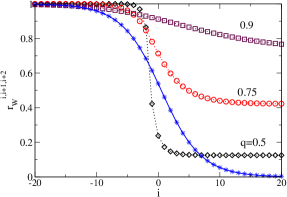
Figure 2: Wick ratio $r_{W}^{i,i+1,i+2}$ for $q=e^{-\beta\Delta}=0.5,0.75$ and $0.9$ as a function of $i$. The asymtotic values for large positive and negative values of $i$ are discussed in the text. The blue “curve” (stars) shows $\bar{n}_{i}$ for $q=0.75$

Realistic values of $q$ differ for the two applications of this model mentioned earlier. For fermions in a 1d harmonic trap the value of the temperature and $\Delta$ can be independently experimentally tuned, i.e. $q$ can be chosen quite arbitrarily. For free fermions with a linearized dispersion $\Delta\sim 1/L$ holds for box of length $L$ and the limit $L\to\infty$ leads to $q\to 1$, implying a Wick ratio of one as in the grand canonical ensemble.

IV.2 Zero bandwidth semiconductor model

A simple model with $M$ degenerate valence band states and $M$ degenerate conduction band states is considered

$$H=\sum_{i=1}^{M}[\epsilon_{v}c_{v,i}^{\dagger}c_{v,i}+(\epsilon_{v}+\Delta)c_{c,i}^{\dagger}c_{c,i}]=\epsilon_{v}{\cal N}_{v}+(\epsilon_{v}+\Delta){\cal N}_{c}~{}.$$ (54)

In the following we put $\epsilon_{v}=0$. Despite the fact that the general case $N\neq M$ is as easily treated as the special case $N=M$, we only present results for the latter in the following. In this case the $N$-fermion ground state is given by the filled valence band. The excited states have $m$ holes in the valence band and $m$ particles in the conduction band. The number of ways to chose $m$ holes in the $N$ valence band states is given by $\binom{N}{m}$. The same result is obtained for the number of ways to put the $m$ particles in the conduction band. Therefore the canonical partition function is given by

$$Z_{N}=\sum_{m=0}^{N}\binom{N}{m}^{2}e^{-m\beta\Delta}~{}.$$ (55)

In order to obtain the mean occupation numbers $\langle n_{\alpha,i}\rangle_{c}$ for $\alpha=v,c$ it is sufficient to calculate $\langle{\cal N}_{c}\rangle_{c}$ as $\langle n_{\alpha,i}\rangle_{c}$ does not depend on $i$ and $\langle{\cal N}_{v}\rangle_{c}+\langle{\cal N}_{c}\rangle_{c}=N$ holds. Introducing the probability distribution $p_{N}(m)$ for the number of electrons in the conduction band the mean occupation of the conduction band is given by

$$\langle{\cal N}_{c}\rangle_{c}=\sum_{m=0}^{N}mp_{N}(m)~{};~{}~{}~{}p_{N}(m)=\frac{1}{Z_{N}}\binom{N}{m}^{2}e^{-m\beta\Delta}~{}.$$ (56)

For not too small values of $q=e^{-\beta\Delta}$ the probability distribution $p_{N}(m)$ for large $N$ resembles a Gaussian distribution as shown in Fig. 3 for $N=50$. For $k_{B}T/\Delta=0.5$ also the grand canonical result is shown for comparison (filled squares) . While its average value is close to the canonical result its width is significantly larger. This is discussed quantitatively later.

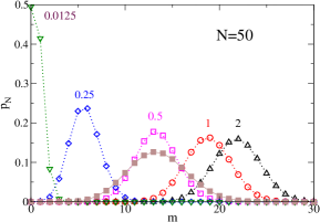
Figure 3: Probability distribution $p_{N}(m)$ for the number $m$ of conduction electrons for the zero bandwidth semiconductor model for $N=50$ and different values of $k_{B}T/\Delta$ indicated at the maximum of the corresponding curve. For $k_{B}T/\Delta=0.5$ also the grand canonical probability distribution is shown (filled squares)

In the grand canonical ensemble the chemical potential lies in the middle of the bands, $\mu=\Delta/2$, for the case $N=M$ considered here. This guarantees $\langle{\cal N}\rangle_{gc}=N$ for all temperatures

$$f_{c}\equiv\langle n_{c,i}\rangle_{gc}=\frac{1}{e^{\beta\Delta/2}+1}=1-\langle n_{v,i}\rangle_{gc}~{}.$$ (57)

This is in contrast to the general case $N\neq M$, in which the chemical potential is temperature dependent. Due to the factorization of $\rho_{gc}^{(0)}$ the conduction band states $c,i$ are independently empty with probability $1-f_{c}$ and filled with probability $f_{c}$. Therefore the grand canonical distribution function is binomial

$$p_{gc}(m)=\binom{N}{m}f_{c}^{m}(1-f_{c})^{N-m}~{}.$$ (58)

with average value $Nf_{c}$ and mean square deviation $Nf_{c}(1-f_{c})$. The transition of a binomial distribution to a Gaussian distribution in the large $N$-limit discussed in textbooks on statistical mechanics. Before addressing the width of $p_{N}(m)$ the average occupation numbers $\langle n_{c,i}\rangle_{c}$ and $f_{c}$ are compared.

In Fig. 4 we show results from the numerical evaluation of $\langle n_{c,i}\rangle_{c}$ using Eq. (56).

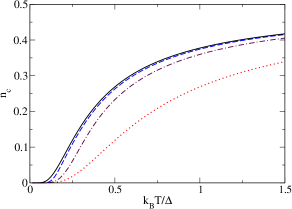
Figure 4: Mean occupation numbers $n_{c}=\langle n_{c,i}\rangle_{c}$ for the zero bandwidth semiconductor model as a function of temperature for different values of $N(=M)$: $N=1$ (dotted), $N=4$ (dashed-dotted) and $N=20$ (dashed). The grand canonical result is presented by the full curve

For small values of $N$ the deviations of the canonical from the grand canonical result are rather large. In the high temperature limit the grand canonical result is approached.

In the extreme low temperature limit $N^{2}e^{-\beta\Delta}\ll 1$ one approximately has $\langle n_{c,i}\rangle\approx Ne^{-\beta\Delta}$ which deviates strongly from the grand canonical result $\approx e^{-\beta\Delta/2}$.

In the large $N$ limit $\langle{\cal N}_{c}\rangle\approx\bar{m}$ where $\bar{m}$ is the position of the maximum of $p_{N}(m)$. Using the Stirling formula $m!\approx\sqrt{2\pi m}(m/e)^{m}$ valid for $m\gg 1$ the variable $m$ in $p_{N}(m)$ can be treated as continuous and the position $\bar{m}$ of the maximum of $p_{N}(m)$ is easily obtained setting the derivative of $p_{N}(m)$ or $\ln(p_{N}(m))$ to zero. With $d~{}\ln m!/dm\approx\ln m$ one obtains

$$\frac{d~{}\ln(p_{N}(m))}{dm} \approx 2~{}[-\ln m+\ln(N-m)]+\ln q$$ (59)

$$= 2~{}\ln\left(\frac{N-m}{m}q^{1/2}\right)~{}.$$

Putting the argument of the logarithm equal to $1$ the position of the maximum follows as $\bar{m}=N/(q^{-1/2}+1)$. With $q=e^{-\beta\Delta}$ and $\langle n_{c,i}\rangle=\langle{\cal N}_{c}\rangle/N$ one finally obtains in the large $N$ limit

$$\langle n_{c,i}\rangle_{c}\to\frac{1}{e^{\beta\Delta/2}+1}=\langle n_{c,i}\rangle_{gc}~{}.$$ (60)

Next we address the expectation values $\langle n_{\alpha,i}n_{\beta,j}\rangle_{c}$ with $i\neq j$ when $\alpha=\beta$, in the canonical ensemble. As they are independent of $i$ and $j$ there are only three different types: the $\langle n_{\alpha,i}n_{\alpha,j}\rangle_{c}$ with $\alpha=v$ or $c$ and $\langle n_{c,i}n_{v,j}\rangle_{c}$. The value of the latter follows easily from Eq. (40). As shown in the following the $\langle n_{\alpha,i}n_{\alpha,j}\rangle_{c}$ are determined by $\langle n_{c,i}n_{v,j}\rangle_{c}$ and $\langle n_{\alpha,i}\rangle_{c}$. This stems from the fact that $\langle{\cal N}_{c}{\cal N}_{v}\rangle_{c}$ can be expressed in terms of $\langle{\cal N}_{\alpha}^{2}\rangle_{c}$ and $\langle{\cal N}_{\alpha}\rangle_{c}$

$$\langle{\cal N}_{c}{\cal N}_{v}\rangle_{c}=\sum_{m=0}^{N}m(N-m)p_{N}(m)=N\langle{\cal N}_{c}\rangle_{c}-\langle{\cal N}_{c}^{2}\rangle_{c}$$ (61)

and with $m(N-m)=N(N-m)-(N-m)^{2}$ the index $c$ on the right hand side can be replaced by $v$. Using $\langle{\cal N}_{c}{\cal N}_{v}\rangle_{c}=N^{2}\langle n_{c,i}n_{v,j}\rangle_{c}$ this implies

$$\langle{\cal N}_{\alpha}^{2}\rangle_{c}=N^{2}(\langle n_{\alpha,i}\rangle_{c}-\langle n_{c,i}n_{v,j}\rangle_{c})~{}.$$ (62)

For $i\neq j$ one has $\langle{\cal N}_{\alpha}^{2}\rangle_{c}=N(N-1)\langle n_{\alpha,i}n_{\alpha,j}\rangle_{c}+N\langle n_{\alpha,i}\rangle_{c}$. This leads to the promised result

$$\langle n_{\alpha,i}n_{\alpha,j}\rangle_{c}=\langle n_{\alpha,i}\rangle_{c}-\frac{N}{N-1}\langle n_{c,i}n_{v,j}\rangle_{c}~{}.$$ (63)

This allows to calculate the $\langle n_{\alpha,i}n_{\alpha,j}\rangle_{c}$ in terms of $\langle n_{\alpha,i}\rangle_{c}$ and $\langle n_{c,i}n_{v,j}\rangle_{c}$ given by Eq. (40)

$$\langle n_{c,i}n_{v,j}\rangle_{c}=\frac{\langle n_{c,i}\rangle_{c}-e^{-\beta\Delta}(1-\langle n_{c,i}\rangle_{c})}{1-e^{-\beta\Delta}}~{}.$$ (64)

If $\langle n_{c,i}n_{v,j}\rangle_{c}$ factorizes in the limit $N\to\infty$ Eq. (63) implies the same for the $\langle n_{\alpha,i}n_{\alpha,j}\rangle_{c}$ for $i\neq j$.

In Fig. 5 we show the Wick ratios $r_{W}^{vv},r_{W}^{cv}$ and $r_{W}^{cc}$ as a function of temperature for $N=4$ and $N=20$. The limiting values for $T\to 0$ and $T\to\infty$ can be understood analytically. At $T=0$ the valence band is completely occupied, i.e. $\langle n_{v,i}\rangle_{c}=1=\langle n_{v,i}n_{v,j}\rangle_{c}$. This implies

$$r_{W}^{vv}(T=0,N)=1~{}.$$ (65)

As at zero temperature the conduction band is empty $\langle n_{c,i}\rangle_{c}=0$, $\langle n_{c,i}n_{v,j}\rangle_{c}=0$ and $\langle n_{c,i}n_{c,j}\rangle_{c}=0$ holds. For the Wick ratios $r_{W}^{cv}$ and $r_{W}^{cc}$ one therefore encounters a $"0/0"$ problem and the limit $T\to 0$ has to be studied.

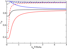
Figure 5: Wick ratios $r_{W}^{vv}$ (blue curves), $r_{W}^{cv}$ (black curves) and $r_{w}^{cc}$ (red curves) as a function of $k_{B}T/\Delta$ for $N=4$ (full curves) and $20$ (dashed curves).

As mentioned earlier, in the extreme low temperature limit $\langle n_{c,i}\rangle_{c}\approx Ne^{-\beta\Delta}\ll 1$ holds. With Eq. (64) this leads to

$$r_{W}^{cv}(T\to 0,N)=1-\frac{1}{N}~{}.$$ (66)

Alternatively this can be obtained by simple combinatorics. As the state $v,j$ is supposed to be occupied there are $N-1$ ways to promote a valence electron to the state $c,i$, leading to $\langle n_{c,i}n_{v,j}\rangle_{c}\approx(N-1)e^{-\beta\Delta}$. With $\langle n_{c,i}\rangle_{c}(1-\langle n_{c,i}\rangle_{c})\approx\langle n_{c,i}\rangle_{c}\approx Ne^{-\beta\Delta}$ this leads to the result in Eq. (66). We finally address the $T\to 0$ limit of $r_{W}^{cc}$. There are $N(N-1)/2$ ways to put two electrons into two prescribed conduction band states, leading to $\langle n_{c,i}n_{c,j}\rangle_{c}\approx N(N-1)e^{-2\beta\Delta}/2$. With the result for $\langle n_{c,i}\rangle_{c}$ one obtains

$$r_{W}^{cc}(T\to 0,N)=\frac{1}{2}\left(1-\frac{1}{N}\right)~{}.$$ (67)

In the high temperature limit $T\to\infty$ simply counting numbers of states determines $\langle n_{\alpha,i}n_{\beta,j}\rangle_{c}$ with $\alpha,i$ differing from $\beta,j$. The number of ways to put two fermions in these two one-particle states and the other $N-2$ particles into the remaining $2N-2$ states is given by $\binom{2N-2}{N-2}$ and the partition function by the total number of possible states $\binom{2N}{N}$. This leads to

$$T\to\infty:~{}~{}~{}~{}r_{W}\to\frac{1-1/N}{1-1/(2N)}$$ (68)

independently of the upper indices. Without the combinatorics just presented, this value of $r_{W}$ can be obtained from Eq. (63) realizing that the $\langle n_{\alpha,i}n_{\beta,j}\rangle_{c}$ with $\alpha,i\neq\beta,j$ are all the same in the infinite temperature limit. One can solve this equation for $x=\langle n_{c,i}n_{v,j}\rangle_{c}=\langle n_{\alpha,i}n_{\alpha,j}\rangle_{c}$ using $\langle n_{\alpha,i}\rangle_{c}=1/2$ and obtains the result of Eq. (68).

In Fig. 6 we show the Wick ratio $r_{W}^{cv}$ as a function of $1/N$ for different values of $k_{B}T/\Delta$. The results lie between the “curves” determined by Eqs. (66) and (68). For large $N$ the infinite temperature result is reached quickly with increasing temperature.

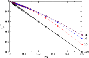
Figure 6: Wick ratio $r_{W}^{cv}$ as a function of $1/N$ for different values of $k_{B}T/\Delta$, indicated at the right edge of the figure. The lower and upper boundary curve of the results are discussed in the text.

We now return to the comparison of the widths of $p_{N}$ and $p_{gc}$ both shown for $k_{B}T/\Delta=0.5$ in Fig. 3. The mean square deviation $\sigma_{c}^{2}$ for both cases is given by

$$\sigma_{c}^{2}=\langle{\cal N}_{c}^{2}\rangle - \langle{\cal N}_{c}\rangle^{2}=N^{2}(\langle n_{c,1}n_{c,2}\rangle-\langle n_{c,1}\rangle^{2})$$ (69)

$$+ N(\langle n_{c,1}\rangle-\langle n_{c,1}n_{c,2}\rangle)~{}.$$

Using Wick’s theorem for the grand canonical case the first term on the right hand side vanishes, leading to $(\sigma_{c}^{2})_{gc}=Nf_{c}(1-f_{c})$, as mentioned earlier.

For the canonical ensemble $\sigma_{c}^{2}$ can be expressed in terms of $\langle n_{c,i}\rangle_{c}$ and $r_{W}^{cc}$ as

$$(\sigma_{c}^{2})_{c}=N^{2}\langle n_{c,1}\rangle_{c}^{2}(r_{W}^{cc}-1)+N(\langle n_{c,1}\rangle_{c}-r_{W}^{cc}\langle n_{c,1}\rangle_{c}^{2})~{}.$$ (70)

For large $N$ and not too low temperatures $r_{W}^{cc}-1\approx-1/(2N)$ holds and the first term of $\sigma_{c}^{2}$ which vanishes in the grand canonical case is approximately given by $-N\langle n_{c1}\rangle_{c}^{2}/2$. To leading order in $N$ the second term is given by $N\langle n_{c1}\rangle_{c}(1-\langle n_{c1}\rangle_{c})\approx Nf_{c}(1-f_{c})$. In the high temperature limit $(\sigma_{c}^{2})_{gc}\approx 2(\sigma_{c}^{2})_{c}$ holds, i.e. the width of $p_{gc}$ is larger by a factor $\sqrt{2}$ than that of $p_{N}$ as can be confirmed in Fig. 3.

V Summary

With an approach similar to Gaudin’s proof of Wick’s theorem for the grand canonical ensemble new results for expectation values of products of occupation numbers of one-particle states with differing one-particle energies were presented for noninteracting fermions in Eqs. (40) and (41). They are valid for the grand canonical as well as the canonical ensemble. To arbitrary order of the products the expectation values are expressed in terms of the average occupation numbers. For two different models it was explicitely shown that these relations allow a deeper undestanding of the deviations from Wick’s theorem in the canonical ensemble which go beyond the purely numerical approaches presented earlier. The deviations can be very large at low temperatures if the product involves occupation number operators of one-particle states which are unocupied at zero temperature.

VI Acknowledgements

The author wants to thank V. Meden and W. Zwerger for a critical reading of the manuscript and useful comments.

Appendix A Alternative derivation of Eq. (40)

Here we show how Eq. (39) for the canonical ensemble could have been found using Eqs. (30) and (31).

In Eq. (31 ) the sums in $s_{l_{1}...l_{m}}^{(k)}$ run from $1$ to $k$. As $j_{i}\geq 1$ for all $i$ it is obvious that the largest value a $j_{i}$ can take is $k-m+1$. As the upper limit of the sums one can also take $\infty$, as the Kronecker delta does its job. Therefore in the following the upper limits of the sums are suppressed.

If one multiplies $s_{l_{1}...l_{m}}^{(k)}$ by $e^{\beta\epsilon_{m}}$ this leads after changing the summation index $j_{m}$ by one to

$$e^{\beta\epsilon_{m}}s^{(k)}_{l_{1}...l_{m}} = \sum_{j_{1}=1}\sum_{j_{2}=1}...\sum_{j_{m}=0}e^{-\beta\sum_{i=1}^{m}j_{i}\epsilon_{l_{i}}}\delta_{j_{1}+...+j_{m},k-1}$$ (71)

$$= s^{(k-1)}_{l_{1}...l_{m-1}}+s^{(k-1)}_{l_{1}..l_{m-1}l_{m}}~{}.$$

In taking the difference with the according expression where one multplies with $e^{\beta\epsilon_{m-1}}$, the second terms cancel and one obtains

$$(e^{\beta\epsilon_{m}}-e^{\beta\epsilon_{m-1}})s^{(k)}_{l_{1}...l_{m}}=s^{(k-1)}_{l_{1}...l_{m-1}}-s^{(k-1)}_{l_{1}...l_{m-2}l_{m}}~{}.$$ (72)

Eq. (71) reads for $m\to m-1$

$$e^{\beta\epsilon_{m-1}}s^{(k)}_{l_{1}...l_{m-1}}=s^{(k-1)}_{l_{1}...l_{m-2}}+s^{(k-1)}_{l_{1}..l_{m-2}l_{m-1}}~{}.$$ (73)

If one performs the corresponding multiplication with $e^{\beta\epsilon_{m}}$ and takes the difference the comparison with Eq. (72) yields

$$(e^{\beta\epsilon_{m}}-e^{\beta\epsilon_{m-1}})s^{(k)}_{l_{1}...l_{m}}=e^{\beta\epsilon_{m-1}}s^{(k)}_{l_{1}...l_{m-1}}-e^{\beta\epsilon_{m}}s^{(k)}_{l_{1}...l_{m-2}l_{m}}~{}.$$ (74)

Inserting this into Eq. (30) leads to

$$(e^{\beta\epsilon_{m-1}}-e^{\beta\epsilon_{m}})\langle n_{l_{1}...l_{m}}\rangle_{c} =$$

$$\langle n_{l_{1}...l_{m-1}}\rangle_{c}e^{\beta\epsilon_{m-1}} - \langle n_{l_{1}...l_{m-2}l_{m}}\rangle_{c}e^{\beta\epsilon_{m}}.$$ (75)

For $\epsilon_{m-1}\neq\epsilon_{m}$ division proves Eq. (39) in a way different from the one presented in section III.

Appendix B Induction step in the proof of Eq. (31)

In this appendix the inductive step in the proof of Eq. (41) is presented. Using the abbreviation $x_{i}=e^{\beta\epsilon_{l_{i}}}$ we assume the formula

$$\langle n_{l_{1}}....n_{l_{m-1}}\rangle=\sum_{i=1}^{m-1}\langle n_{l_{i}}\rangle\prod_{j(\neq i)}^{m-1}\frac{x_{i}}{x_{i}-x_{j}}$$ (76)

to be correct. By putting this into the recursion formula Eq. (39)

$$\langle P^{(m)}\rangle=\frac{\langle P^{(m-2)}n_{l_{m-1}}\rangle x_{m-1}-\langle P^{(m-2)}n_{l_{m}}\rangle x_{m}}{x_{m-1}-x_{m}}~{}.$$ (77)

we show that formula Eq. (76) also holds for $m$. In both $\langle P^{(m-2)}n_{l_{k}}\rangle$ with $k=m-1$ and $k=m$ all occupation number operators $n_{l_{j}}$ with $j\leq m-2$ occur. In contrast $n_{l_{m-1}}$ and $n_{l_{m}}$ only appear in one of the two expectation values in Eq (77 ). A term proportional to $\langle n_{l_{m-1}}\rangle$ only results from the first expectation value. Its contribution to $\langle P^{(m)}\rangle$ is given by

$$\frac{x_{m-1}}{x_{m-1}-x_{m}}\prod_{j=1}^{m-2}\frac{x_{m-1}}{x_{m-1}-x_{j}}=\prod_{j(\neq m-1)}^{m}\frac{x_{m-1}}{x_{m-1}-x_{j}}~{}.$$ (78)

The term proportional to $\langle n_{l_{m}}\rangle$ results from the second expectation value

$$-\frac{x_{m}}{x_{m-1}-x_{m}}\prod_{j=1}^{m-2}\frac{x_{m}}{x_{m}-x_{j}}=\prod_{j(\neq m)}^{m}\frac{x_{m}}{x_{m}-x_{j}}~{}.$$ (79)

For the terms proportional to $\langle n_{l_{j}}\rangle$ with $j\leq m-2$ it is sufficient to consider a single example e.g. $\langle n_{l_{1}}\rangle$. With $p_{m-2}^{(1)}=\prod_{j=2}^{m-2}x_{1}/(x_{1}-x_{j})$ and using the recursion relation Eq. (77) the contribution proportional to $\langle n_{l_{1}}\rangle$ in $\langle P^{(m)}\rangle$ is given by

$$\frac{1}{x_{m-1}-x_{m}}p_{m-2}^{(1)}\left(\frac{x_{1}x_{m-1}}{x_{1}-x_{m-1}}-\frac{x_{1}x_{m}}{x_{1}-x_{m}}\right)$$ (80)

$$= \prod_{j=2}^{m}\frac{x_{1}}{x_{1}-x_{j}}~{}.$$

This completes the inductive step for the proof of Eq. (41).

The proof that $\langle P^{(m)}\rangle$ completely factorizes for the grand canonical average is again easier by induction. For $m=2$ one has

$$\langle n_{l_{1}}n_{l_{2}}\rangle_{gc} = \frac{x_{1}\langle n_{l_{1}}\rangle_{gc}-x_{2}\langle n_{l_{2}}\rangle_{gc}}{x_{1}-x_{2}}$$

$$= \frac{x_{1}(x_{2}+1)-x_{2}(x_{1}+1)}{(x_{1}-x_{2})(x_{1}+1)(x_{2}+1)}=\langle n_{l_{1}}\rangle_{gc}\langle n_{l_{2}}\rangle_{gc}$$

Now we assume that $\langle P^{(m-1)}\rangle_{gc}$ completely factorizes and use Eq. (77) for the induction step. This assumption implies $\langle P^{(m-2)}n_{l_{k}}\rangle_{gc}$ with $k=m-1$ and $k=m$ factorizes $\langle P^{(m-2)}n_{l_{k}}\rangle_{gc}=\langle P^{(m-2)}\rangle_{gc}\langle n_{l_{k}}\rangle_{gc}$. This implies with Eq. (77)

$$\langle n_{l_{1}}....n_{l_{m}}\rangle_{gc} = \langle P^{(m-2)}\rangle_{gc}\frac{x_{m-1}\langle n_{l_{m-1}}\rangle_{gc}-x_{m-1}\langle n_{l_{m-1}}\rangle_{gc}}{x_{m-1}-x_{m}}$$ (82)

$$= \prod_{i=1}^{m}\langle n_{l_{i}}\rangle_{gc}~{}.$$

This proof is certainly more involved than the one in subsection IIIb.

References

- (1) W.J. Mullin and J.P. Fernandez, Am. J. Phys. 71, 661-669 (2003)
- (2) V.V. Kocharovski, Vl.V. Kocharovski, M. Holthaus, C.H. Raymond Oui, A. Svidzinsky, W. Ketterle, and M.O. Scully, Adv. At. Mol. Opt. Phys. 53, 2911-411 (2006)
- (3) K. Tsutsui and T. Kita, J. Phys. Soc. Jpn 85, 114603-114608 (2016)
- (4) M. Gaudin, Nucl. Phys. 15, 89-91 (1960)
- (5) A. Fetter, J. Walecka, Quantum Theory of Many Particle Systems , McGraw-Hill 1971
- (6) H. Schmidt, Z. Phys. 134, 430-431 (1953)
- (7) P. Borrmann and G. Franke, J. Chem. Phys. 98, 2484-2485 (1993)
- (8) P. Borrmann, J. Harting, O. Mülken, and E.R. Hilf, Phys. Rev. A60, 1519-1521 (1999)
- (9) A.N. Wenz, G. Zürn, S. Murmann, I. Brouzos, T. Lompe, and S. Jochim, Science 342, 457-460 (2013)
- (10) K. Schönhammer, Am. J. Phys. 68, 1032-1037 (2000)
- (11) F. D. M. Haldane, J. Phys. C. 14, 2585-2919 (1981)
- (12) K. Schönhammer and V. Meden, Am. J. Phys. 64, 1168-1176 (1996)