Dynamic Semiparametric Models for Expected Shortfall (and Value-at-Risk)

Abstract

Expected Shortfall (ES) is the average return on a risky asset conditional on the return being below some quantile of its distribution, namely its Value-at-Risk (VaR). The Basel III Accord, which will be implemented in the years leading up to 2019, places new attention on ES, but unlike VaR, there is little existing work on modeling ES. We use recent results from statistical decision theory to overcome the problem of “elicitability” for ES by jointly modelling ES and VaR, and propose new dynamic models for these risk measures. We provide estimation and inference methods for the proposed models, and confirm via simulation studies that the methods have good finite-sample properties. We apply these models to daily returns on four international equity indices, and find the proposed new ES-VaR models outperform forecasts based on GARCH or rolling window models.

Keywords: Risk management, tails, crashes, forecasting, generalized autoregressive score.

J.E.L. codes: G17, C22, G32, C58.

1 Introduction

The financial crisis of 2007-08 and its aftermath led to numerous changes in financial market regulation and banking supervision. One important change appears in the Third Basel Accord (Basel Committee, 2010), where new emphasis is placed on “Expected Shortfall” (ES) as a measure of risk, complementing, and in parts substituting, the more-familiar Value-at-Risk (VaR) measure. Expected Shortfall is the expected return on an asset conditional on the return being below a given quantile of its distribution, namely its VaR. That is, if $Y_{t}$ is the return on some asset over some horizon (e.g., one day or one week) with conditional (on information set $\mathcal{F}_{t-1}$) distribution $F_{t}$, which we assume to be strictly increasing with finite mean, the $\alpha$-level VaR and ES are:

$$\mathrm{ES}_{t} =\mathbb{E}\left[Y_{t}|Y_{t}\leq\mathrm{VaR}_{t},\mathcal{F}_{t-1}\right]$$ (1)

$$\text{where \ \ }\mathrm{VaR}_{t} =F_{t}^{-1}\left(\alpha\right)\text{, \ for }\alpha\in\left(0,1\right)$$ (2)

$$\text{and \ \ }Y_{t}|\mathcal{F}_{t-1} \thicksim F_{t}$$ (3)

As Basel III is implemented worldwide (implementation is expected to occur in the period leading up to January 1${}^{\text{st}}$, 2019), ES will inevitably gain, and require, increasing attention from risk managers and banking supervisors and regulators. The new “market discipline” aspects of Basel III mean that ES and VaR will be regularly disclosed by banks, and so a knowledge of these measures will also likely be of interest to these banks’ investors and counter-parties.

There is, however, a paucity of empirical models for expected shortfall. The large literature on volatility models (see Andersen et al. (2006) for a review) and VaR models (see Komunjer (2013) and McNeil et al. (2015)), have provided many useful models for these measures of risk. However, while ES has long been known to be a “coherent” measure of risk (Artzner, et al. 1999), in contrast with VaR, the literature contains relatively few models for ES; some exceptions are discussed below. This dearth is perhaps in part because regulatory interest in this risk measure is only recent, and perhaps also due to the fact that this measure is not “elicitable.” A risk measure (or statistical functional more generally) is said to be “elicitable” if there exists a loss function such that the measure is the solution to minimizing the expected loss. For example, the mean is elicitable using the quadratic loss function, and VaR is elicitable using the piecewise-linear or “tick” loss function. Having such a loss function is a stepping stone to building dynamic models for these quantities. We use recent results from Fissler and Ziegel (2016), who show that ES is jointly elicitable with VaR, to build new dynamic models for ES and VaR.

This paper makes three main contributions. Firstly, we present some novel dynamic models for ES and VaR, drawing on the GAS framework of Creal, et al. (2013), as well as successful models from the volatility literature, see Andersen et al. (2006). The models we propose are semiparametric in that they impose parametric structures for the dynamics of ES and VaR, but are completely agnostic about the conditional distribution of returns (aside from regularity conditions required for estimation and inference). The models proposed in this paper are related to the class of “CAViaR” models proposed by Engle and Manganelli (2004a), in that we directly parameterize the measure(s) of risk that are of interest, and avoid the need to specify a conditional distribution for returns. The models we consider make estimation and prediction fast and simple to implement. Our semiparametric approach eliminates the need to specify and estimate a conditional density, thereby removing the possibility that such a model is misspecified, though at a cost of a loss of efficiency compared with a correctly specified density model.

Our second contribution is asymptotic theory for a general class of dynamic semiparametric models for ES and VaR. This theory is an extension of results for VaR presented in Weiss (1991) and Engle and Manganelli (2004a), and draws on identification results in Fissler and Ziegel (2016) and results for M-estimators in Newey and McFadden (1994). We present conditions under which the estimated parameters of the VaR and ES models are consistent and asymptotically normal, and we present a consistent estimator of the asymptotic covariance matrix. We show via an extensive Monte Carlo study that the asymptotic results provide reasonable approximations in realistic simulation designs. In addition to being useful for the new models we propose, the asymptotic theory we present provides a general framework for other researchers to develop, estimate, and evaluate new models for VaR and ES.

Our third contribution is an extensive application of our new models and estimation methods in an out-of-sample analysis of forecasts of ES and VaR for four international equity indices over the period January 1990 to December 2016. We compare these new models with existing methods from the literature across a range of tail probability values $\left(\alpha\right)$ used in risk management. We use Diebold and Mariano (1995) tests to identify the best-performing models for ES and VaR, and we present simple regression-based methods, related to those of Engle and Manganelli (2004a) and Nolde and Ziegel (2017), to “backtest” the ES forecasts.

Some work on expected shortfall estimation and prediction has appeared in the literature, overcoming the problem of elicitability in different ways: Engle and Manganelli (2004b) discuss using extreme value theory, combined with GARCH or CAViaR dynamics, to obtain forecasts of ES. Cai and Wang (2008) propose estimating VaR and ES based on nonparametric conditional distributions, while Taylor (2008) and Gschöpf et al. (2015) estimate models for “expectiles” (Newey and Powell, 1987) and map these to ES. Zhu and Galbraith (2011) propose using flexible parametric distributions for the standardized residuals from models for the conditional mean and variance. Drawing on Fissler and Ziegel (2016), we overcome the problem of elicitability more directly, and open up new directions for ES modeling and prediction.

In recent independent work, Taylor (2017) proposes using the asymmetric Laplace distribution to jointly estimate dynamic models for VaR and ES. He shows the intriguing result that the negative log-likelihood of this distribution corresponds to one of the loss functions presented in Fissler and Ziegel (2016), and thus can be used to estimate and evaluate such models. Unlike our paper, Taylor (2017) provides no asymptotic theory for his proposed estimation method, nor any simulation studies of its reliability. However, given the link he presents, the theoretical results we present below can be used to justify ex post the methods of his paper.

The remainder of the paper is structured as follows. In Section 2 we present new dynamic semiparametric models for ES and VaR and compare them with the main existing models for ES and VaR. In Section 3 we present asymptotic distribution theory for a generic dynamic semiparametric model for ES and VaR, and in Section 4 we study the finite-sample properties of the asymptotic theory in some realistic Monte Carlo designs. Section 5 we apply the new models to daily data on four international equity indices, and compare these models both in-sample and out-of-sample with existing models. Section 6 concludes. Proofs and additional technical details are presented in the appendix, and a supplemental web appendix contains detailed proofs and additional analyses.

2 Dynamic models for ES and VaR

In this section we propose some new dynamic models for expected shortfall (ES) and Value-at-Risk (VaR). We do so by exploiting recent work in Fissler and Ziegel (2016) which shows that these variables are elicitable jointly, despite the fact that ES was known to be not elicitable separately, see Gneiting (2011a). The models we propose are based on the GAS framework of Creal, et al. (2013) and Harvey (2013), which we briefly review in Section 2.2 below.

2.1 A consistent scoring rule for ES and VaR

Fissler and Ziegel (2016) show that the following class of loss functions (or “scoring rules”), indexed by the functions $G_{1}$ and $G_{2},$ is consistent for VaR and ES. That is, minimizing the expected loss using any of these loss functions returns the true VaR and ES. In the functions below, we use the notation $v$ and $e$ for VaR and ES.

$$L_{FZ}\left(Y,v,e;\alpha,G_{1},G_{2}\right) =\left(\mathbf{1}\left\{Y\leq v\right\}-\alpha\right)\left(G_{1}\left(v\right)-G_{1}\left(Y\right)+\frac{1}{\alpha}G_{2}\left(e\right)v\right)$$ (4)

$$-G_{2}\left(e\right)\left(\frac{1}{\alpha}\mathbf{1}\left\{Y\leq v\right\}Y-e\right)-\mathcal{G}_{2}\left(e\right)$$

where $G_{1}$ is weakly increasing, $G_{2}$ is strictly increasing and strictly positive, and $\mathcal{G}_{2}^{\prime}=G_{2}.$ We will refer to the above class as “FZ loss functions.” Minimizing any member of this class yields VaR and ES:

$$\left(\mathrm{VaR}_{t},\mathrm{ES}_{t}\right)=\arg\min_{\left(v,e\right)}~{}\mathbb{E}_{t-1}\left[L_{FZ}\left(Y_{t},v,e;\alpha,G_{1},G_{2}\right)\right]$$ (5)

Using the FZ loss function for estimation and forecast evaluation requires choosing $G_{1}$ and $G_{2}.$ We choose these so that the loss function generates loss differences (between competing forecasts) that are homogeneous of degree zero. This property has been shown in volatility forecasting applications to lead to higher power in Diebold-Mariano (1995) tests in Patton and Sheppard (2009). Nolde and Ziegel (2017) show that there does not generally exist an FZ loss function that generates loss differences that are homogeneous of degree zero. However, zero-degree homogeneity may be attained by exploiting the fact that, for the values of $\alpha$ that are of interest in risk management applications (namely, values ranging from around 0.01 to 0.10), we may assume that $\mathrm{ES}_{t}<0$ a.s. $\forall~{}t.$ The following proposition shows that if we further impose that $\mathrm{VaR}_{t}<0~{}$a.s. $\forall~{}t,$ then, up to irrelevant location and scale factors, there is only one FZ loss function that generates loss differences that are homogeneous of degree zero. The fact that the $L_{FZ0}$ loss function defined below is unique has the added benefit that there are, of course, no remaining shape or tuning parameters to be specified.

Proposition 1

Define the FZ loss difference for two forecasts $\left(v_{1t},e_{1t}\right)$ and $\left(v_{2t},e_{2t}\right)$ as $L_{FZ}\left(Y_{t},v_{1t},e_{1t};\alpha,G_{1},G_{2}\right)-L_{FZ}\left(Y_{t},v_{2t},e_{2t};\alpha,G_{1},G_{2}\right).$ Under the assumption that VaR and ES are both strictly negative, the loss differences generated by a FZ loss function are homogeneous of degree zero iff $G_{1}(x)=0$ and $G_{2}(x)=1/x.$ The resulting “FZ0” loss function is:

$$L_{FZ0}\left(Y,v,e;\alpha\right)=-\frac{1}{\alpha e}\mathbf{1}\left\{Y\leq v\right\}\left(v-Y\right)+\frac{v}{e}+\log\left(-e\right)-1$$ (6)

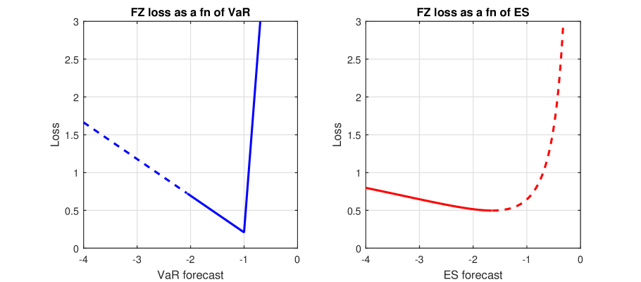
Figure 1: This figure plots the FZ0 loss function when $Y=-1$ and $\alpha=0.05.$ In the left panel we fix $e=-2.06$ and vary $v,$ in the right panel we fix $v=-1.64$ and vary $e.$ Values where $v<e$ are indicated with a dashed line.

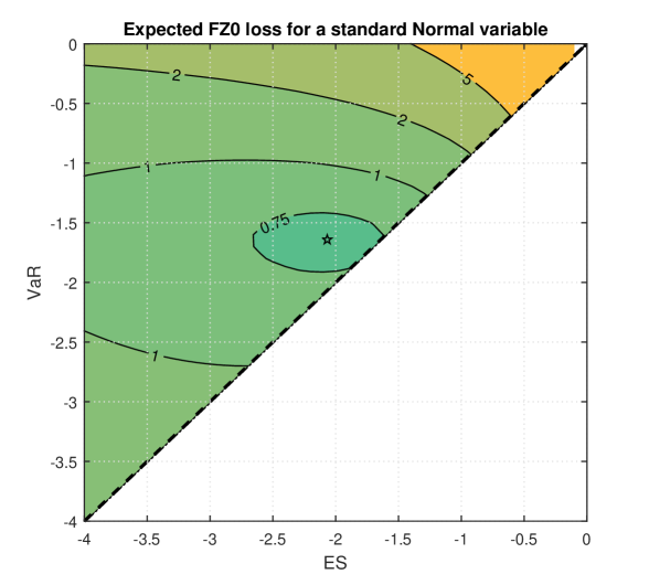
Figure 2: Contours of expected FZ0 loss when the target variable is standard Normal. Only values where ES$<$VaR$<$0 are considered. The optimal value is marked with a star.

All proofs are presented in Appendix A. In Figure 1 we plot $L_{FZ0}$ when $Y=-1.$ In the left panel we fix $e=-2.06$ and vary $v,$ and in the right panel we fix $v=-1.64$ and vary $e.$ (These values for $\left(v,e\right)$ are the $\alpha=0.05$ VaR and ES from a standard Normal distribution.) As neither of these are the complete loss function, the minimum is not zero in either panel. The left panel shows that the implied VaR loss function resembles the “tick” loss function from quantile estimation, see Komunjer (2005) for example. In the right panel we see that the implied ES loss function resembles the “QLIKE” loss function from volatility forecasting, see Patton (2011) for example. In both panels, values of $\left(v,e\right)$ where $v<e$ are presented with a dashed line, as by definition $\mathrm{ES}_{t}$ is below $\mathrm{VaR}_{t},$ and so such values that would never be considered in practice. In Figure 2 we plot the contours of expected FZ0 loss for a standard Normal random variable. The minimum value, which is attained when $\left(v,e\right)=\left(-1.64,-2.06\right)$, is marked with a star, and we see that the “iso-expected loss” contours are convex. Fissler (2017) shows that convexity of iso-expected loss contours holds more generally for the FZ0 loss function under any distribution with finite first moments, unique $\alpha$-quantiles, continuous densities, and negative ES.

[ INSERT FIGURES 1 AND 2 ABOUT HERE ]

With the FZ0 loss function in hand, it is then possible to consider semiparametric dynamic models for ES and VaR:

$$\left(\mathrm{VaR}_{t},\mathrm{ES}_{t}\right)=\left(v\left(\mathbf{Z}_{t-1};\mathbf{\theta}\right),e\left(\mathbf{Z}_{t-1};\mathbf{\theta}\right)\right)$$ (7)

that is, where the true VaR and ES are some specified parametric functions of elements of the information set, $\mathbf{Z}_{t-1}\in\mathcal{F}_{t-1}.$ The parameters of this model are estimated via:

$$\mathbf{\hat{\theta}}_{T}=\arg\min_{\mathbf{\theta}}~{}\frac{1}{T}{\displaystyle\sum\nolimits_{t=1}^{T}}L_{FZ0}\left(Y_{t},v\left(\mathbf{Z}_{t-1};\mathbf{\theta}\right),e\left(\mathbf{Z}_{t-1};\mathbf{\theta}\right);\alpha\right)$$ (8)

Such models impose a parametric structure on the dynamics of VaR and ES, through their relationship with lagged information, but require no assumptions, beyond regularity conditions, on the conditional distribution of returns. In this sense, these models are semiparametric. Using theory for M-estimators (see White (1994) and Newey and McFadden (1994) for example) we establish in Section 3 below the asymptotic properties of such estimators. Before doing so, we first consider some new dynamic specifications for ES and VaR.

2.2 A GAS model for ES and VaR

One of the challenges in specifying a dynamic model for a risk measure, or any other quantity of interest, is the mapping from lagged information to the current value of the variable. Our first proposed specification for ES and VaR draws on the work of Creal, et al. (2013) and Harvey (2013), who proposed a general class of models called “generalized autoregressive score” (GAS) models by the former authors, and “dynamic conditional score” models by the latter author. In both cases the models start from an assumption that the target variable has some parametric conditional distribution, where the parameter (vector) of that distribution follows a GARCH-like equation. The forcing variable in the model is the lagged score of the log-likelihood, scaled by some positive definite matrix, a common choice for which is the inverse Hessian. This specification nests many well known models, including ARMA, GARCH (Bollerslev, 1986) and ACD (Engle and Russell, 1998) models. See Koopman et al. (2016) for an overview of GAS and related models.

We adopt this modeling approach and apply it to our M-estimation problem. In this application, the forcing variable is a function of the derivative and Hessian of the $L_{FZ0}$ loss function rather than a log-likelihood. We will consider the following GAS(1,1) model for ES and VaR:

$$\left[\begin{array}[c]{c}v_{t+1}\\ e_{t+1}\end{array}\right]=\mathbf{w+B}\left[\begin{array}[c]{c}v_{t}\\ e_{t}\end{array}\right]+\mathbf{AH}_{t}^{-1}\mathbf{\nabla}_{t}$$ (9)

where $\mathbf{w}$ is a $\left(2\times 1\right)$ vector and $\mathbf{B}$ and $\mathbf{A}$ are $\left(2\times 2\right)$ matrices. The forcing variable in this specification is comprised of two components, the first is the score:

$$\mathbf{\nabla}_{t} \equiv\left[\begin{array}[c]{c}\partial L_{FZ0}\left(Y_{t},v_{t},e_{t};\alpha\right)/\partial v_{t}\\ \partial L_{FZ0}\left(Y_{t},v_{t},e_{t};\alpha\right)/\partial e_{t}\end{array}\right]=\left[\begin{array}[c]{c}\frac{1}{\alpha v_{t}e_{t}}\lambda_{v,t}\\ \frac{-1}{\alpha e_{t}^{2}}\left(\lambda_{v,t}+\alpha\lambda_{e,t}\right)\end{array}\right]$$ (14)

$$\text{where \ \ }\lambda_{v,t} \equiv-v_{t}\left(\mathbf{1}\left\{Y_{t}\leq v_{t}\right\}-\alpha\right)$$ (15)

$$\lambda_{e,t} \equiv\frac{1}{\alpha}\mathbf{1}\left\{Y_{t}\leq v_{t}\right\}Y_{t}-e_{t}$$ (16)

The scaling matrix, $\mathbf{H}_{t},$ is related to the Hessian:

$$\mathbf{I}_{t}\equiv\left[\begin{array}[c]{cc}\frac{\partial^{2}\mathbb{E}_{t-1}\left[L_{FZ0}\left(Y_{t},v_{t},e_{t}\right)\right]}{\partial v_{t}^{2}}&\frac{\partial^{2}\mathbb{E}_{t-1}\left[L_{FZ0}\left(Y_{t},v_{t},e_{t}\right)\right]}{\partial v_{t}\partial e_{t}}\\ \bullet&\frac{\partial^{2}\mathbb{E}_{t-1}\left[L_{FZ0}\left(Y_{t},v_{t},e_{t}\right)\right]}{\partial e_{t}^{2}}\end{array}\right]=\left[\begin{array}[c]{cc}-\frac{f_{t}\left(v_{t}\right)}{\alpha e_{t}}&0\\ 0&\frac{1}{e_{t}^{2}}\end{array}\right]$$ (17)

The second equality above exploits the fact that $\partial^{2}\mathbb{E}_{t-1}\left[L_{FZ0}\left(Y_{t},v_{t},e_{t};\alpha\right)\right]/\partial v_{t}\partial e_{t}=0$ under the assumption that the dynamics for VaR and ES are correctly specified. The first element of the matrix $\mathbf{I}_{t}$ depends on the unknown conditional density of $Y_{t}.$ We would like to avoid estimating this density, and we approximate the term $f_{t}\left(v_{t}\right)$ as being proportional to $v_{t}^{-1}.$ This approximation holds exactly if $Y_{t}$ is a zero-mean location-scale random variable, $Y_{t}=\sigma_{t}\eta_{t}$, where $\eta_{t}\thicksim iid~{}F_{\eta}\left(0,1\right),$ as in that case we have:

$$f_{t}\left(v_{t}\right)=f_{t}\left(\sigma_{t}v_{\alpha}\right)=\frac{1}{\sigma_{t}}f_{\eta}\left(v_{\alpha}\right)\equiv k_{\alpha}\frac{1}{v_{t}}$$ (18)

where $k_{\alpha}\equiv v_{\alpha}f_{\eta}\left(v_{\alpha}\right)$ is a constant with the same sign as $v_{t}$. We define $\mathbf{H}_{t}$ to equal $\mathbf{I}_{t}$ with the first element replaced using the approximation in the above equation. The forcing variable in our GAS model for VaR and ES then becomes:

$$\mathbf{H}_{t}^{-1}\mathbf{\nabla}_{t}=\left[\begin{array}[c]{c}\frac{-1}{k_{\alpha}}\lambda_{v,t}\\ \frac{-1}{\alpha}\left(\lambda_{v,t}+\alpha\lambda_{e,t}\right)\end{array}\right]$$ (19)

Notice that the second term in the model is a linear combination of the two elements of the forcing variable, and since the forcing variable is premultiplied by a coefficient matrix, say $\mathbf{\tilde{A}},$ we can equivalently use

$$\mathbf{\tilde{A}H}_{t}^{-1}\mathbf{\nabla}_{t} =\mathbf{A\lambda}_{t}$$ (20)

$$\text{where \ }\mathbf{\lambda}_{t} \equiv\left[\lambda_{v,t},\lambda_{e,t}\right]^{\prime}$$

We choose to work with the $\mathbf{A\lambda}_{t}$ parameterization, as the two elements of this forcing variable $\left(\lambda_{v,t},\lambda_{e,t}\right)$ are not directly correlated, while the elements of $\mathbf{H}_{t}^{-1}\mathbf{\nabla}_{t}$ are correlated due to the overlapping term ($\lambda_{v,t}$) appearing in both elements. This aids the interpretation of the results of the model without changing its fit.

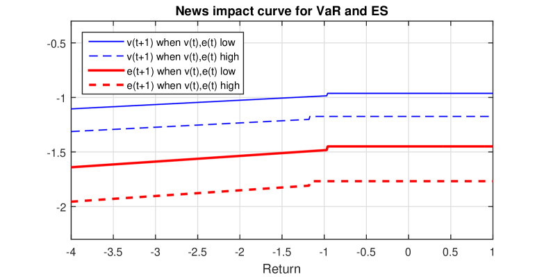
Figure 3: This figure shows the values of VaR and ES as a function of the lagged return, when the lagged values of VaR and ES are either low (10% below average) or high (10% above average). The function is based on the estimated parameters for daily S&P 500 returns.

To gain some intuition for how past returns affect current forecasts of ES and VaR in this model, consider the “news impact curve” of this model, which presents $\left(v_{t+1},e_{t+1}\right)$ as a function of $Y_{t}$ through its impact on $\mathbf{\lambda}_{t}\equiv\left[\lambda_{v,t},\lambda\,_{e,t}\right]^{\prime},$ holding all other variables constant. Figure 3 shows these two curves for $\alpha=0.05,$ using the estimated parameters for this model when applied to daily returns on the S&P 500 index (details are presented in Section 5 below). We consider two values for the “current” value of $\left(v,e\right)$: 10% above and below the long-run average for these variables. We see that for values where $Y_{t}>v_{t},$ the news impact curves are flat, reflecting the fact that on those days the value of the realized return does not enter the forcing variable. When $Y_{t}\leq v_{t},$ we see that ES and VaR react linearly to $Y$ and this reaction is through the $\lambda_{e,t}$ forcing variable; the reaction through the $\lambda_{v,t}$ forcing variable is a simple step (down) in both of these risk measures.

[ INSERT FIGURE 3 ABOUT HERE ]

2.3 A one-factor GAS model for ES and VaR

The specification in Section 2.2 allows ES and VaR to evolve as two separate, correlated, processes. In many risk forecasting applications, a useful simpler model is one based on a structure with only one time-varying risk measure, e.g. volatility. We will consider a one-factor model in this section, and will name the model in Section 2.2 a “two-factor” GAS model.

Consider the following one-factor GAS model for ES and VaR, where both risk measures are driven by a single variable, $\kappa_{t}$:

$$v_{t} =a\exp\left\{\kappa_{t}\right\}$$ (21)

$$e_{t} =b\exp\left\{\kappa_{t}\right\}\text{, \ where }b<a<0$$

$$\text{and \ }\kappa_{t} =\omega+\beta\kappa_{t-1}+\gamma H_{t-1}^{-1}s_{t-1}$$

The forcing variable, $H_{t-1}^{-1}s_{t-1},$ in the evolution equation for $\kappa_{t}$ is obtained from the FZ0 loss function, plugging in $\left(a\exp\left\{\kappa_{t}\right\},b\exp\left\{\kappa_{t}\right\}\right)$ for $\left(v_{t},e_{t}\right)$.  Using details provided in Appendix B.2, we find that the score and Hessian are:

$$s_{t} \equiv\frac{\partial L_{FZ0}\left(Y_{t},a\exp\left\{\kappa_{t}\right\},b\exp\left\{\kappa_{t}\right\};\alpha\right)}{\partial\kappa}=-\frac{1}{e_{t}}\left(\frac{1}{\alpha}\mathbf{1}\left\{Y_{t}\leq v_{t}\right\}Y_{t}-e_{t}\right)$$ (22)

$$\text{and \ }I_{t} \equiv\frac{\partial^{2}\mathbb{E}_{t-1}\left[L_{FZ0}\left(Y_{t},a\exp\left\{\kappa_{t}\right\},b\exp\left\{\kappa_{t}\right\};\alpha\right)\right]}{\partial\kappa_{t}^{2}}=\frac{\alpha-k_{\alpha}a_{\alpha}}{\alpha}$$ (23)

where $k_{\alpha}$ is a negative constant and $a_{\alpha}$ lies between zero and one. The Hessian, $I_{t}$, turns out to be a constant in this case, and since we estimate a free coefficient on our forcing variable, we simply set $H_{t}$ to one. Note that the VaR score, $\lambda_{v,t}=\partial L/\partial v$, turns out to drop out from the forcing variable. Thus the one-factor GAS model for ES and VaR becomes:

$$\kappa_{t}=\omega+\beta\kappa_{t-1}+\gamma\frac{-1}{b\exp\left\{\kappa_{t-1}\right\}}\left(\frac{1}{\alpha}\mathbf{1}\left\{Y_{t-1}\leq a\exp\left\{\kappa_{t-1}\right\}\right\}Y_{t-1}-b\exp\left\{\kappa_{t-1}\right\}\right)$$ (24)

Using the FZ loss function for estimation, we are unable to identify $\omega,$ as there exists $\left(\tilde{\omega},\tilde{a},\tilde{b}\right)\neq\left(\omega,a,b\right)$ such that both triplets yield identical sequences of ES and VaR estimates, and thus identical values of the objective function. We fix $\omega=0$ and forfeit identification of the level of the series for $\kappa_{t}$, though we of course retain the ability to model and forecast ES and VaR. Foreshadowing the empirical results in Section 5, we find that this one-factor GAS model outperforms the two-factor GAS model in out-of-sample forecasts for most of the asset return series that we study.

2.4 Existing dynamic models for ES and VaR

As noted in the introduction, there is a relative paucity of dynamic models for ES and VaR, but there is not a complete absence of such models. The simplest existing model is based on a simple rolling window estimate of these quantities:

$$\widehat{\mathrm{VaR}}_{t} =\widehat{\text{{Quantile}}}\left\{Y_{s}\right\}_{s=t-m}^{t-1}$$ (25)

$$\widehat{\mathrm{ES}}_{t} =\frac{1}{\alpha m}{\displaystyle\sum\limits_{s=t-m}^{t-1}}Y_{s}\mathbf{1}\left\{Y_{s}\leq\widehat{\mathrm{VaR}}_{s}\right\}$$

where $\widehat{\text{{Quantile}}}\left\{Y_{s}\right\}_{s=t-m}^{t-1}$ denotes the sample quantile of $Y_{s}$ over the period $s\in\left[t-m,t-1\right].$ Common choices for the window size, $m,$ include 125, 250 and 500, corresponding to six months, one year and two years of daily return observations respectively.

A more challenging competitor for the new ES and VaR models proposed in this paper are those based on ARMA-GARCH dynamics for the conditional mean and variance, accompanied by some assumption for the distribution of the standardized residuals. These models all take the form:

$$Y_{t} =\mu_{t}+\sigma_{t}\eta_{t}$$ (26)

$$\eta_{t} \thicksim iid~{}F_{\eta}\left(0,1\right)$$

where $\mu_{t}$ and $\sigma_{t}^{2}$ are specified to follow some ARMA and GARCH model, and $F_{\eta}\left(0,1\right)$ is some arbitrary, strictly increasing, distribution with mean zero and variance one. What remains is to specify a distribution for the standardized residual, $\eta_{t}$. Given a choice for $F_{\eta},$ VaR and ES forecasts are obtained as:

$$v_{t} =\mu_{t}+a\sigma_{t}\text{, \ \ where \ }a=F_{\eta}^{-1}\left(\alpha\right)$$ (27)

$$e_{t} =\mu_{t}+b\sigma_{t}\text{, \ \ where \ }b=\mathbb{E}\left[\eta_{t}|\eta_{t}\leq a\right]$$

Two parametric choices for $F_{\eta}$ are common in the literature:

$$\eta_{t} \thicksim iid~{}N\left(0,1\right)$$ (28)

$$\eta_{t} \thicksim iid~{}Skew~{}t\left(0,1,\nu,\lambda\right)$$

There are various skew $t$ distributions used in the literature; in the empirical analysis below we use that of Hansen (1994). A nonparametric alternative is to estimate the distribution of $\eta_{t}$ using the empirical distribution function (EDF), an approach that is also known as “filtered historical simulation,” and one that is perhaps the best existing model for ES, see the survey by Engle and Manganelli (2004b). We consider all of these models in our empirical analysis in Section 5.

2.5 GARCH and ES/VaR estimation

In this section we consider two extensions of the models presented above, in an attempt to combine the success and parsimony of GARCH models with this paper’s focus on ES and VaR forecasting.

2.5.1 Estimating a GARCH model via FZ minimization

If an ARMA-GARCH model, including the specification for the distribution of standardized residuals, is correctly specified for the conditional distribution of an asset return, then maximum likelihood is the most efficient estimation method, and should naturally be adopted. If, on the other hand, we consider an ARMA-GARCH model only as a useful approximation to the true conditional distribution, then it is no longer clear that MLE is optimal. In particular, if the application of the model is to ES and VaR forecasting, then we might be able to improve the fitted ARMA-GARCH model by estimating the parameters of that model via FZ loss minimization, as discussed in Section 2.1. This estimation method is related to one discussed in Remark 1 of Francq and Zakoïan (2015).

Consider the following model for asset returns:

$$Y_{t} =\kappa_{t}\eta_{t}\text{, \ \ }\eta_{t}\thicksim iid~{}F_{\eta}\left(0,1\right)$$ (29)

$$\kappa_{t}^{2} =\omega+\beta\kappa_{t-1}^{2}+\gamma Y_{t-1}^{2}$$

The variable $\kappa_{t}^{2}$ is the conditional variance and is assumed to follow a GARCH(1,1) process. This model implies a structure analogous to the one-factor GAS model presented in Section 2.3, as we find:

$$v_{t} =a\cdot\kappa_{t}\text{, \ where }a=F_{\eta}^{-1}\left(\alpha\right)$$ (30)

$$e_{t} =b\cdot\kappa_{t}\text{, \ where }b=\mathbb{E}\left[\eta|\eta\leq a\right]$$

Some further results on VaR and ES in dynamic location-scale models are presented in Appendix B.3. To apply this model to VaR and ES forecasting, we also have to estimate the VaR and ES of the standardized residual, denoted $\left(a,b\right).$ Rather than estimating the parameters of this model using (Q)MLE, we consider here estimating the via FZ loss minimization. As in the one-factor GAS model, $\omega$ is unidentified and we set it to one, so the parameter vector to be estimated is $\left(\beta,\gamma,a,b\right)$. This estimation approach leads to a fitted GARCH model that is tailored to provide the best-fitting ES and VaR forecasts, rather than the best-fitting volatility forecasts.

2.5.2 A hybrid GAS/GARCH model

Finally, we consider a direct combination of the forcing variable suggested by a GAS structure for a one-factor model of returns, described in equation (24), with the successful GARCH model for volatility. We specify:

$$Y_{t} =\exp\left\{\kappa_{t}\right\}\eta_{t}\text{, \ \ }\eta_{t}\thicksim iid~{}F_{\eta}\left(0,1\right)$$ (31)

$$\kappa_{t} =\omega+\beta\kappa_{t-1}+\gamma\left(-\frac{1}{e_{t-1}}\left(\frac{1}{\alpha}\mathbf{1}\left\{Y_{t-1}\leq v_{t-1}\right\}Y_{t-1}-e_{t-1}\right)\right)+\delta\log\left|Y_{t-1}\right|$$

The variable $\kappa_{t}$ is the log-volatility, identified up to scale. As the latent variable in this model is log-volatility, we use the lagged log absolute return rather than the lagged squared return, so that the units remain in line for the evolution equation for $\kappa_{t}$. There are five parameters in this model $\left(\beta,\gamma,\delta,a,b\right),$ and we estimate them using FZ loss minimization.

3 Estimation of dynamic models for ES and VaR

This section presents asymptotic theory for the estimation of dynamic ES and VaR models by minimizing FZ loss. Given a sample of observations $\left(y_{1},\cdots,y_{T}\right)$ and a constant $\alpha\in\left(0,0.5\right)$, we are interested in estimating and forecasting the conditional $\alpha$ quantile (VaR) and corresponding expected shortfall of $Y_{t}$. Suppose $Y_{t}$ is a real-valued random variable that has, conditional on information set $\mathcal{F}_{t-1}$, distribution function $F_{t}\left(\cdot|\mathcal{F}_{t-1}\right)\$and corresponding density function $f_{t}\left(\cdot|\mathcal{F}_{t-1}\right)$. Let $v_{1}(\mathbf{\theta}^{0})$ and $e_{1}(\mathbf{\theta}^{0})$ be some initial conditions for VaR and ES and let $\mathcal{F}_{t-1}=\sigma\{Y_{t-1},\mathbf{X}_{t-1},\cdots,Y_{1},\mathbf{X}_{1}\},$ where $\mathbf{X}_{t}$ is a vector of exogenous variables or predetermined variables, be the information set available for forecasting $Y_{t}$. The vector of unknown parameters to be estimated is $\mathbf{\theta}^{0}\in\Theta\subset\mathbb{R}^{p}$.

The conditional VaR and ES of $Y_{t}$ at probability level $\alpha,$ that is $\mathrm{VaR}_{\alpha}\left(Y_{t}|\mathcal{F}_{t-1}\right)$ and $\mathrm{ES}_{\alpha}\left(Y_{t}|\mathcal{F}_{t-1}\right)$, are assumed to follow some dynamic model:

$$\left[\begin{array}[c]{c}\mathrm{VaR}_{\alpha}\left(Y_{t}|\mathcal{F}_{t-1}\right)\\ \mathrm{ES}_{\alpha}\left(Y_{t}|\mathcal{F}_{t-1}\right)\end{array}\right]=\left[\begin{array}[c]{c}v(Y_{t-1},\mathbf{X}_{t-1},\cdots,Y_{1},\mathbf{X}_{1};\mathbf{\theta}^{0})\\ e(Y_{t-1},\mathbf{X}_{t-1},\cdots,Y_{1},\mathbf{X}_{1};\mathbf{\theta}^{0})\end{array}\right]\equiv\left[\begin{array}[c]{c}v_{t}(\mathbf{\theta}^{0})\\ e_{t}(\mathbf{\theta}^{0})\end{array}\right],~{}t=1,\cdots,T,$$ (32)

The unknown parameters are estimated as:

$$\mathbf{\hat{\theta}}_{T} \equiv\arg\min_{\mathbf{\theta}\in\Theta}~{}L_{T}(\mathbf{\theta})$$ (33)

$$\text{where \ }L_{T}(\mathbf{\theta}) =\frac{1}{T}\sum_{t=1}^{T}L_{FZ0}\left(Y_{t},v_{t}\left(\mathbf{\theta}\right),e_{t}\left(\mathbf{\theta}\right);\alpha\right)$$

and the FZ loss function $L_{FZ0}$ is defined in equation (6). Below we provide conditions under which estimation of these parameters via FZ loss minimization leads to a consistent and asymptotically normal estimator, with standard errors that can be consistently estimated.

Assumption 1

(A) $L\left(Y_{t},v_{t}\left(\mathbf{\theta}\right),e_{t}\left(\mathbf{\theta}\right);\alpha\right)$ obeys the uniform law of large numbers.

(B)(i) $\Theta$ is a compact subset of $\mathbb{R}^{p}$ for $p<\infty.$ (ii)$\{Y_{t}\}_{t=1}^{\infty}$ is a strictly stationary process. Conditional on all the past information $\mathcal{F}_{t-1}$, the distribution of $Y_{t}$ is $F_{t}\left(\cdot|\mathcal{F}_{t-1}\right)$ which, for all $t,$ belongs to a class of distribution functions on $\mathbb{R}$ with finite first moments and unique $\alpha$-quantiles. (iii) $\forall t$, both $v_{t}(\mathbf{\theta})$ and $e_{t}(\mathbf{\theta})$ are $\mathcal{F}_{t-1}$-measurable and continuous in $\mathbf{\theta}$. (iv) If $\Pr\left[v_{t}(\mathbf{\theta})=v_{t}(\mathbf{\theta}^{0})\cap e_{t}(\mathbf{\theta})=e_{t}(\mathbf{\theta}^{0})\right]=1~{}\forall~{}t$, then $\mathbf{\theta=\theta}^{0}.$

Theorem 1 (Consistency)

Under Assumption 1, $\mathbf{\hat{\theta}}_{T}\overset{p}{\rightarrow}\mathbf{\theta}^{0}$ as $T\rightarrow\infty.$

The proof of Theorem 1, provided in Appendix A, is straightforward given Theorem 2.1 of Newey and McFadden (1994) and Corollary 5.5 of Fissler and Ziegel (2016). Note that a variety of uniform laws of large numbers (our Assumption 1(A)) are available for the time series applications we consider here, see Andrews (1987) and Pötscher and Prucha (1989) for example. Zwingmann and Holzmann (2016) show that if the $\alpha$-quantile is not unique (violating our Assumption 1(B)(iii)), then the convergence rate and asymptotic distribution of $\left(\hat{v}_{T},\hat{e}_{T}\right)$ are non-standard, even in a setting with $iid$ data. We do not consider such problematic cases here.

We next turn to the asymptotic distribution of our parameter estimator. In the assumptions below, $K$ denotes a finite constant that can change from line to line, and we use $\left\|\mathbf{x}\right\|$ to denote the Euclidean norm of a vector $\mathbf{x.}$

Assumption 2

(A) For all $t$, we have (i) $v_{t}(\mathbf{\theta})$ and $e_{t}(\mathbf{\theta})$ are twice continuously differentiable in $\mathbf{\theta}$, (ii) $v_{t}(\mathbf{\theta}^{0})\leq 0$.

(B) For all $t$, we have (i) Conditional on all the past information $\mathcal{F}_{t-1}$, $Y_{t}$ has a continuous density $f_{t}\left(\cdot|\mathcal{F}_{t-1}\right)$ that satisfies $f_{t}(y|\mathcal{F}_{t-1})\leq K<\infty$ and $\left|f_{t}(y_{1}|\mathcal{F}_{t-1})-f_{t}(y_{2}|\mathcal{F}_{t})\right|\leq K\left|y_{1}-y_{2}\right|$, (ii) $\mathbb{E}\left[\left|Y_{t}\right|^{4+\delta}\right]\leq K<\infty$, for some $0<\delta<1$.

(C) There exists a neighborhood of $\mathbf{\theta}^{0}$, $\mathcal{N}\left(\mathbf{\theta}^{0}\right)$, such that for all $t$ we have (i) $|1/e_{t}(\theta)|\leq K<\infty$, $\forall~{}\theta\in\mathcal{N}\left(\mathbf{\theta}^{0}\right),$ (ii) there exist some (possibly stochastic) $\mathcal{F}_{t-1}$-measurable functions $V(\mathcal{F}_{t-1})$, $V_{1}(\mathcal{F}_{t-1})$, $H_{1}(\mathcal{F}_{t-1})$, $V_{2}(\mathcal{F}_{t-1})$, $H_{2}(\mathcal{F}_{t-1})$ which satisfy $\forall\mathbf{\theta}\in\mathcal{N}(\mathbf{\theta}^{0})$: $|v_{t}(\mathbf{\theta})|\leq V(\mathcal{F}_{t-1})$, $\left\|\nabla v_{t}(\mathbf{\theta})\right\|\leq V_{1}(\mathcal{F}_{t-1})$, $\left\|\nabla e_{t}(\mathbf{\theta})\right\|\leq H_{1}(\mathcal{F}_{t-1})$, $\left\|\nabla^{2}v_{t}(\mathbf{\theta})\right\|\leq V_{2}(\mathcal{F}_{t-1})$, and $\left\|\nabla^{2}e_{t}(\mathbf{\theta})\right\|\leq H_{2}(\mathcal{F}_{t-1})$.

(D) For some $0<\delta<1$ and for all $t$ we have (i) $\mathbb{E}\left[V_{1}(\mathcal{F}_{t-1})^{3+\delta}\right]$, $\mathbb{E}\left[H_{1}(\mathcal{F}_{t-1})^{3+\delta}\right]$, $\mathbb{E}\left[V_{2}(\mathcal{F}_{t-1})^{\frac{3+\delta}{2}}\right]$, $\mathbb{E}\left[H_{2}(\mathcal{F}_{t-1})^{\frac{3+\delta}{2}}\right]\leq K$, (ii) $\mathbb{E}\left[V(\mathcal{F}_{t-1})^{2+\delta}V_{1}(\mathcal{F}_{t-1})H_{1}(\mathcal{F}_{t-1})^{2+\delta}\right]\leq K$,(iii) $\mathbb{E}\left[H_{1}(\mathcal{F}_{t-1})^{1+\delta}H_{2}(\mathcal{F}_{t-1})\left|Y_{t}\right|^{2+\delta}\right]$, $\mathbb{E}\left[H_{1}(\mathcal{F}_{t-1})^{3+\delta}\left|Y_{t}\right|^{2+\delta}\right]\leq K.$

(E) The matrix $\mathbf{D}_{T}$ defined in Theorem 2 has eigenvalues bounded below by a positive constant for $T$ sufficiently large.

(F) The sequence $\{T^{-1/2}\sum_{t=1}^{T}g_{t}(\mathbf{\theta}^{0})\}$ obeys the CLT, where

$$g_{t}(\mathbf{\theta}) =\frac{\partial L\left(Y_{t},v_{t}\left(\mathbf{\theta}\right),e_{t}\left(\mathbf{\theta}\right);\alpha\right)}{\partial\mathbf{\theta}}$$ (34)

$$= \nabla v_{t}(\mathbf{\theta})^{\prime}\frac{1}{-e_{t}(\mathbf{\theta})}\left(\frac{1}{\alpha}\mathbf{1}\left\{Y_{t}\leq v_{t}(\mathbf{\theta})\right\}-1\right)$$ (35)

$$+ \nabla e_{t}(\mathbf{\theta})^{\prime}\frac{1}{e_{t}(\mathbf{\theta})^{2}}\left(\frac{1}{\alpha}\mathbf{1}\left\{Y_{t}\leq v_{t}(\mathbf{\theta})\right\}(v_{t}(\mathbf{\theta})-Y_{t})-v_{t}(\mathbf{\theta})+e_{t}(\mathbf{\theta})\right)$$

(G) $\left\{Y_{t}\right\}$ is $\alpha$-mixing of size $-2q/\left(q-2\right)$ for some $q>2.$

Most of the above assumptions are standard. Assumption 2(A)(i) imposes that the VaR is negative, but given our focus on the left-tail $\left(\alpha\leq 0.5\right)$ of asset returns, this is not likely a binding constraint. Assumptions 2(B),(C) and (E) are similar to those in Engle and Manganelli (2004a). Assumption 2(B)(ii) requires at least $4+\delta$ moments of returns to exist, however 2(D) may actually increase the number of required moments, depending on the VaR-ES model employed. For the familiar GARCH(1,1) process, used in our simulation study, it can be shown that we only need to assume that $4+\delta$ moments exist. Assumption 2(F) allows for some CLT for mixing data to be invoked, and 2(G) is a standard assumption on the time series dependence of the data.

Theorem 2 (Asymptotic Normality)

Under Assumptions 1 and 2, we have

$$\sqrt{T}\mathbf{A}_{T}^{-1/2}\mathbf{D}_{T}(\mathbf{\hat{\theta}}_{T}-\mathbf{\theta}^{0})\overset{d}{\rightarrow}N(0,I)\text{ as }T\rightarrow\infty$$ (36)

where

$$\mathbf{D}_{T} =\mathbb{E}\left[T^{-1}\sum_{t=1}^{T}\frac{f_{t}\left(v_{t}(\mathbf{\theta}^{0})|\mathcal{F}_{t-1}\right)}{-e_{t}(\mathbf{\theta}^{0})\alpha}\nabla v_{t}(\mathbf{\theta}^{0})^{\prime}\nabla v_{t}(\mathbf{\theta}^{0})+\frac{1}{e_{t}(\mathbf{\theta}^{0})^{2}}\nabla e_{t}(\mathbf{\theta}^{0})^{\prime}\nabla e_{t}(\mathbf{\theta}^{0})\right]$$ (37)

$$\mathbf{A}_{T} =\mathbb{E}\left[T^{-1}\sum_{t=1}^{T}g_{t}(\mathbf{\theta}^{0})g_{t}(\mathbf{\theta}^{0})^{\prime}\right]$$ (38)

and $g_{t}$ is defined in Assumption 2(F).

An outline of the proof of this theorem is given in Appendix A, and the detailed lemmas underlying it are provided in the supplemental appendix. The proof of Theorem 2 builds on Huber (1967), Weiss (1991) and Engle and Manganelli (2004a), who focused on the estimation of quantiles.

Finally, we present a result for estimating the asymptotic covariance matrix of $\mathbf{\hat{\theta}}_{T},$ thereby enabling the reporting of standard errors and confidence intervals.

Assumption 3

(A) The deterministic positive sequence $c_{T}$ satisfies $c_{T}=o(1)$ and $c_{T}^{-1}=o(T^{1/2})$.

(B)(i) $T^{-1}\sum_{t=1}^{T}g_{t}(\mathbf{\theta}^{0})g_{t}(\mathbf{\theta}^{0})^{{}^{\prime}}-\mathbf{A}_{T}\overset{p}{\rightarrow}{\mathbf{0}}$, where $\mathbf{A}_{T}$ is defined in Theorem 2.

(ii) $T^{-1}\sum_{t=1}^{T}\frac{1}{e_{t}(\theta^{0})^{2}}\nabla e_{t}(\mathbf{\theta}^{0})^{\prime}\nabla e_{t}(\mathbf{\theta}^{0})-\mathbb{E}[T^{-1}\sum_{t=1}^{T}\frac{1}{e_{t}(\mathbf{\theta}^{0})^{2}}\nabla e_{t}(\mathbf{\theta}^{0})^{\prime}\nabla e_{t}(\mathbf{\theta}^{0})]\overset{p}{\rightarrow}{\mathbf{0}}$.

(iii) $T^{-1}\sum_{t=1}^{T}\frac{f_{t}(v_{t}(\mathbf{\theta}^{0})|\mathcal{F}_{t-1})}{-e_{t}(\mathbf{\theta}^{0})\alpha}\nabla v_{t}(\mathbf{\theta}^{0})^{\prime}\nabla v_{t}(\mathbf{\theta}^{0})-\mathbb{E}[T^{-1}\sum_{t=1}^{T}\frac{f_{t}(v_{t}(\mathbf{\theta}^{0})|\mathcal{F}_{t-1})}{-e_{t}(\mathbf{\theta}^{0})\alpha}\nabla v_{t}(\mathbf{\theta}^{0})^{\prime}\nabla v_{t}(\mathbf{\theta}^{0})]\overset{p}{\rightarrow}{\mathbf{0}}$.

Theorem 3

Under Assumptions 1-3, $\mathbf{\hat{A}}_{T}-\mathbf{A}_{T}\overset{p}{\rightarrow}\mathbf{0}$ and $\mathbf{\hat{D}}_{T}-\mathbf{D}_{T}\overset{p}{\rightarrow}\mathbf{0}$, where

$$\mathbf{\hat{A}}_{T}= T^{-1}\sum_{t=1}^{T}g_{t}(\mathbf{\hat{\theta}}_{T})g_{t}(\mathbf{\hat{\theta}}_{T})^{\prime}$$

$$\mathbf{\hat{D}}_{T}= T^{-1}\sum_{t=1}^{T}\left\{\frac{1}{2c_{T}}\mathbf{1}\left\{\left|y_{t}-v_{t}\left(\mathbf{\hat{\theta}}_{T}\right)\right|<c_{T}\right\}\frac{\nabla^{\prime}v_{t}\left(\mathbf{\hat{\theta}}_{T}\right)\nabla v_{t}\left(\mathbf{\hat{\theta}}_{T}\right)}{-\alpha e_{t}\left(\mathbf{\hat{\theta}}_{T}\right)}+\frac{\nabla^{\prime}e_{t}\left(\mathbf{\hat{\theta}}_{T}\right)\nabla e_{t}\left(\mathbf{\hat{\theta}}_{T}\right)}{e_{t}^{2}\left(\mathbf{\hat{\theta}}_{T}\right)}\right\}$$

This result extends Theorem 3 in Engle and Manganelli (2004a) from dynamic VaR models to dynamic joint models for VaR and ES. The key choice in estimating the asymptotic covariance matrix is the bandwidth parameter in Assumption 3(A). In our simulation study below we set this to $T^{-1/3}$ and we find that this leads to satisfactory finite-sample properties.

The results here extend some very recent work in the literature: Dimitriadis and Bayer (2017) consider VaR-ES regression, but focus on $iid$ data and linear specifications. Barendse (2017) considers “interquantile expectation regression,” which nests VaR-ES regression as a special case. He allows for time series data, but imposes that the models are linear. Our framework allows for time series data and nonlinear models.

4 Simulation study

In this section we investigate the finite-sample accuracy of the asymptotic theory for dynamic ES and VaR models presented in the previous section. For ease of comparison with existing studies of related models, such as volatility and VaR models, we consider a GARCH(1,1) for the DGP, and estimate the parameters by FZ-loss minimization. Specifically, the DGP is

$$Y_{t} =\sigma_{t}\eta_{t}$$ (39)

$$\sigma_{t}^{2} =\omega+\beta\sigma_{t-1}^{2}+\gamma Y_{t-1}^{2}$$

$$\eta_{t} \thicksim iid~{}F_{\eta}\left(0,1\right)$$ (40)

We set the parameters of this DGP to $\left(\omega,\beta,\gamma\right)=\left(0.05,0.9,0.05\right).$ We consider two choices for the distribution of $\eta_{t}$: a standard Normal, and the standardized skew $t$ distribution of Hansen (1994), with degrees of freedom and skewness parameters in the latter set to $\left(5,-0.5\right).$ Under this DGP, the ES and VaR are proportional to $\sigma_{t}$,  with

$$\left(\mathrm{VaR}_{t}^{\alpha},\mathrm{ES}_{t}^{\alpha}\right)=\left(a_{\alpha},b_{\alpha}\right)\sigma_{t}$$ (41)

We make the dependence of the coefficients of proportionality $\left(a_{\alpha},b_{\alpha}\right)$ on $\alpha$ explicit here, as we consider a variety of values of $\alpha$ in this simulation study: $\alpha\in\left\{0.01,0.025,0.05,0.10,0.20\right\}.$ Interest in VaR and ES from regulators focuses on the smaller of these values of $\alpha,$ but we also consider the larger values to better understand the properties of the asymptotic approximations at various points in the tail of the distribution.

For a standard Normal distribution, with CDF and PDF denoted $\Phi$ and $\phi,$ we have:

$$a_{\alpha} =\Phi^{-1}\left(\alpha\right)$$ (42)

$$b_{\alpha} =-\phi\left(\Phi^{-1}\left(\alpha\right)\right)/\alpha$$

For Hansen’s skew $t$ distribution we can obtain $a_{\alpha}$ from the inverse CDF, but no closed-form expression for $b_{\alpha}$ is available; we instead use a simulation of 10 million $iid$ draws to estimate it. As noted above, FZ loss minimization does not allow us to identify $\omega$ in the GARCH model, and in our empirical work we set this parameter to 1. To facilitate comparisons of the accuracy of estimates of $\left(a_{\alpha},b_{\alpha}\right)$ in our simulation study we instead set $\omega$ at its true value. This is done without loss of generality and merely eases the presentation of the results. To match our empirical application, we replace the parameter $a_{\alpha}$ with $c_{\alpha}=a_{\alpha}/b_{\alpha},$ and so our parameter vector becomes $\left[\beta,\gamma,b_{\alpha},c_{\alpha}\right].$

We consider two sample sizes, $T\in\left\{2500,5000\right\}$ corresponding to 10 and 20 years of daily returns respectively. These large sample sizes enable us to consider estimating models for quantiles as low as 1%, which are often used in risk management. We repeat all simulations 1000 times.

Table 1 presents results for the estimation of this model on standard Normal innovations, and Table 2 presents corresponding results for skew $t$ innovations. The top row of each panel present the true parameter values, with the latter two parameters changing across $\alpha.$ The second row presents the median estimated parameter across simulations, and the third row presents the average bias in the estimated parameter. Both of these measures indicate that the parameter estimates are nicely centered on the true parameter values. The penultimate row presents the cross-simulation standard deviations of the estimated parameters, and we observe that these decrease with the sample size and increase as we move further into the tails (i.e., as $\alpha$ decreases), both as expected. Comparing the standard deviations across Tables 1 and 2, we also note that they are higher for skew $t$ innovations than Normal innovations, again as expected.

The last row in each panel presents the coverage probabilities for 95% confidence intervals for each parameter, constructed using the estimated standard errors, with bandwidth parameter $c_{T}=\left\lfloor T^{-1/3}\right\rfloor$. For $\alpha\geq 0.05$ we see that the coverage is reasonable, ranging from around 0.88 to 0.96. For $\alpha=0.025$ or $\alpha=0.01$ the coverage tends to be too low, particularly for the smaller sample size. Thus some caution is required when interpreting the standard errors for the models with the smallest values of $\alpha.$ In Table S1 of the Supplemental Appendix we present results for (Q)MLE for the GARCH model corresponding to the results in Tables 1 and 2, using the theory of Bollerslev and Wooldridge (1992). In Tables S2 and S3 we present results for CAViaR estimation of this model, using the “tick” loss function and the theory of Engle and Manganelli (2004a). We find that (Q)MLE has better finite sample properties than FZ minimization, but CAViaR estimation has slightly worse properties than FZ minimization.

[INSERT TABLES 1 AND 2 ABOUT HERE ]

In Table 3 we compare the efficiency of FZ estimation relative to (Q)MLE and to CAViaR estimation, for the parameters that all three estimation methods have in common, namely $\left[\beta,\gamma\right].$ As expected, when the innovations are standard Normal, FZ estimation is substantially less efficient than MLE, however when the innovations are skew $t$ the loss in efficiency drops and for some values of $\alpha$ FZ estimation is actually more efficient than QMLE. This switch in the ranking of the competing estimators is qualitatively in line with results in Francq and Zakoïan (2015). In Panel B of Table 3, we see that FZ estimation is generally, though not uniformly, more efficient than CAViaR estimation.

In many applications, interest is more focused on the forecasted values of VaR and ES than the estimated parameters of the models. To study this, Table 4 presents results on the accuracy of the fitted VaR and ES estimates for the three estimation methods: (Q)MLE, CAViaR and FZ estimation. To obtain estimates of VaR and ES from the (Q)ML estimates, we follow common empirical practice and compute the sample VaR and ES of the estimated standardized residuals. In the first column of each panel we present the mean absolute error (MAE) from (Q)MLE, and in the next two columns we present the relative MAE of CAViaR and FZ to (Q)MLE. Table 4 reveals that (Q)MLE is the most accurate estimation method. Averaging across values of $\alpha,$ CAViaR is about 40% worse for Normal innovations, and 24% worse for skew $t$ innovations, while FZ fares somewhat better, being about 30% worse for Normal innovations and 16% worse for skew $t$ innovations. The superior performance of (Q)MLE is not surprising when the innovations are Normal, as that corresponds to (full) maximum likelihood, which has maximal efficiency. Weighing against the loss in FZ estimation efficiency is the robustness that FZ estimation offers relative to QML. For applications even further from Normality, e.g. with time-varying skewness or kurtosis, the loss in efficiency of QML is likely even greater.

[INSERT TABLES 3 AND 4 ABOUT HERE ]

Overall, these simulation results show that the asymptotic results of the previous section provide reasonable approximations in finite samples, with the approximations improving for larger sample sizes and less extreme values of $\alpha.$ Compared with MLE, estimation by FZ loss minimization is generally less accurate, while it is generally more accurate than estimation using the CAViaR approach of Engle and Manganelli (2004a). The latter outperformance is likely attributable to the fact that FZ estimation draws on information from two tail measures, VaR and ES, while CAViaR was designed to only model VaR.

5 Forecasting equity index ES and VaR

We now apply the models discussed in Section 2 to the forecasting of ES and VaR for daily returns on four international equity indices. We consider the S&P 500 index, the Dow Jones Industrial Average, the NIKKEI 225 index of Japanese stocks, and the FTSE 100 index of UK stocks. Our sample period is 1 January 1990 to 31 December 2016, yielding between 6,630 and 6,805 observations per series (the exact numbers vary due to differences in holidays and market closures). In our out-of-sample analysis, we use the first ten years for estimation, and reserve the remaining 17 years for evaluation and model comparison.

Table 5 presents full-sample summary statistics on these four return series. Average annualized returns range from -2.7% for the NIKKEI to 7.2% for the DJIA, and annualized standard deviations range from 17.0% to 24.7%. All return series exhibit mild negative skewness (around -0.15) and substantial kurtosis (around 10). The lower two panels of Table 5 present the sample VaR and ES for four choices of $\alpha.$

Table 6 presents results from standard time series models estimated on these return series over the in-sample period (Jan 1990 to Dec 1999). In the first panel we present the estimated parameters of the optimal ARMA$\left(p,q\right)$ models, where the choice of $\left(p,q\right)$ is made using the BIC. The $R^{2}$ values from the optimal models never rises above 1%, consistent with the well-known lack of predictability of these series. The second panel presents the parameters of the GARCH(1,1) model for conditional variance, and the lower panel presents the estimated parameters the skew $t$ distribution applied to the standardized residuals. All of these parameters are broadly in line with values obtained by other authors for these or similar series.

[ INSERT TABLES 5 AND 6 ABOUT HERE ]

5.1 In-sample estimation

We now present estimates of the parameters of the models presented in Section 2, along with standard errors computed using the theory from Section 3. In the interests of space, we only report the parameter estimates for the S&P 500 index for $\alpha=0.05$. The two-factor GAS model based on the FZ0 loss function is presented in the left panel of Table 7. This model allows for separate dynamics in VaR and ES, and we present the parameters for each of these risk measures in separate columns. We observe that the persistence of these processes is high, with the estimated $b$ parameters equal to 0.973 and 0.977, similar to the persistence found in GARCH models (e.g., see Table 6). The model-implied average values of VaR and ES are -2.001 and -2.556, similar to the sample values of these measures reported in Table 5. We also observe that in neither equation is the coefficient on $\lambda_{v}$ statistically significant: the $t$-statistics on $a_{v}$ are both well below one. The coefficients on $\lambda_{e}$ are both larger, and more significant (the $t$-statistics are 1.58 and 1.75), indicating that the forcing variable from the ES part of the FZ0 loss function is the more informative component. However, the overall imprecision of the four coefficients on the forcing variables is suggestive that this model is over-parameterized.

The right panel of Table 7 shows three one-factor models for ES and VaR. The first is the one-factor GAS model, which is nested in the two-factor model presented in the left panel. We see a slight loss in fit (the average loss is slightly greater) but the parameters of this model are estimated with greater precision. The one-factor GAS model fits slightly better than the GARCH model estimated via FZ loss minimization (reported in the penultimate column). The “hybrid” model, augmenting the one-factor GAS model with a GARCH-type forcing variable, fits better than the other one-factor models, and also better than the larger two-factor GAS model, and we observe that the coefficient on the GARCH forcing variable $\left(\delta\right)$ is significantly different from zero (with a $t$-statistic of 2.07).

[ INSERT TABLE 7 ABOUT HERE ]

5.2 Out-of-sample forecasting

We now turn to the out-of-sample (OOS) forecast performance of the models discussed above, as well as some competitor models from the existing literature. We will focus initially on the results for $\alpha=0.05,$ given the focus on that percentile in the extant VaR literature. (Results for other values of $\alpha$ are considered later, with details provided in the supplemental appendix.) We will consider a total of ten models for forecasting ES and VaR. Firstly, we consider three rolling window methods, using window lengths of 125, 250 and 500 days. We next consider ARMA-GARCH models, with the ARMA model orders selected using the BIC, and assuming that the distribution of the innovations is standard Normal or skew $t,$ or estimating it nonparametrically using the sample ES and VaR of the estimated standardized residuals. Finally we consider four new semiparametric dynamic models for ES and VaR: the two-factor GAS model presented in Section 2.2, the one-factor GAS model presented in Section 2.3, a GARCH model estimated using FZ loss minimization, and the “hybrid” GAS/GARCH model presented in Section 2.5. We estimate these models using the first ten years as our in-sample period, and retain those parameter estimates throughout the OOS period.

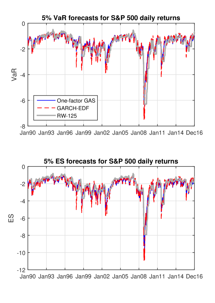
Figure 4: This figure plots the estimated 5% Value-at-Risk (VaR) and Expected Shortfall (ES) for daily returns on the S&P 500 index, over the period January 1990 to December 2016. The estimates are based on a one-factor GAS model, a GARCH model, and a rolling window using 125 observations.

In Figure 4 below we plot the fitted 5% ES and VaR for the S&P 500 return series, using three models: the rolling window model using a window of 125 days, the GARCH-EDF model, and the one-factor GAS model. This figure covers both the in-sample and out-of-sample periods. The figure shows that the average ES was estimated at around -2%, rising as high as around -1% in the mid 90s and mid 00s, and falling to its most extreme values of around -10% during the financial crisis in late 2008. Thus, like volatility, ES fluctuates substantially over time.

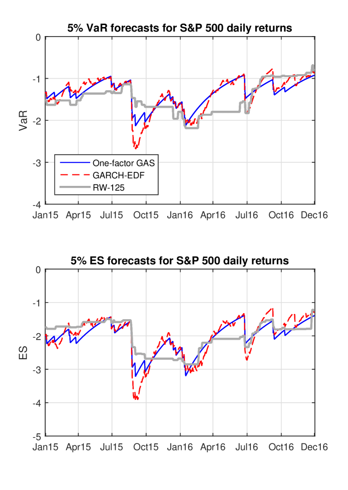
Figure 5: This figure plots the estimated 5% Value-at-Risk (VaR) and Expected Shortfall (ES) for daily returns on the S&P 500 index, over the period January 2015 to December 2016. The estimates are based on a one-factor GAS model, a GARCH model, and a rolling window using 125 observations.

Figure 5 zooms in on the last two years of our sample period, to better reveal the differences in the estimates from these models. We observe the usual step-like movements in the rolling window estimate of VaR and ES, as the more extreme observations enter and leave the estimation window. Comparing the GARCH and GAS estimates, we see how they differ in reacting to returns: the GARCH estimates are driven by lagged squared returns, and thus move stochastically each day. The GAS estimates, on the other hand, only use information from returns when the VaR is violated, and on other days the estimates revert deterministically to the long-run mean. This generates a smoother time series of VaR and ES estimates. We investigate below which of these estimates provides a better fit to the data.

[ INSERT FIGURES 4 AND 5 ABOUT HERE ]

The left panel of Table 8 presents the average OOS losses, using the FZ0 loss function from equation (6), for each of the ten models, for the four equity return series. The lowest values in each column are highlighted in bold, and the second-lowest are in italics. We observe that the one-factor GAS model, labelled FZ1F, is the preferred model for the two US equity indices, while the Hybrid model is the preferred model for the NIKKEI and FTSE indices. The worst model is the rolling window with a window length of 500 days.

While average losses are useful for an initial look at OOS forecast performance, they do not reveal whether the gains are statistically significant. Table 9 presents Diebold-Mariano t-statistics on the loss differences, for the S&P 500 index. Corresponding tables for the other three equity return series are presented in Table S4 of the supplemental appendix. The tests are conducted as “row model minus column model” and so a positive number indicates that the column model outperforms the row model. The column “FZ1F” corresponding to the one-factor GAS model contains all positive entries, revealing that this model out-performed all competing models. This outperformance is strongly significant for the comparisons to the rolling window forecasts, as well as the GARCH model with Normal innovations. The gains relative to the GARCH model with skew $t$ or nonparametric innovations are not significant, with DM $t$-statistics of 1.48 and 1.16 respectively. Similar results are found for the best models for each of the other three equity return series. Thus the worst models are easily separated from the better models, but the best few models are generally not significantly different.

[ INSERT TABLES 8 AND 9 ABOUT HERE ]

To complement the study of the relative performance of these models for ES and VaR, we now consider goodness-of-fit tests for the OOS forecasts of VaR and ES. Under correct specification of the model for VaR and ES, we know that

$$\mathbb{E}_{t-1}\left[\begin{array}[c]{c}\partial L_{FZ0}\left(Y_{t},v_{t},e_{t};\alpha\right)/\partial v_{t}\\ \partial L_{FZ0}\left(Y_{t},v_{t},e_{t};\alpha\right)/\partial e_{t}\end{array}\right]=0$$ (43)

and we note that this implies that $\mathbb{E}_{t-1}\left[\lambda_{v,t}\right]=\mathbb{E}_{t-1}\left[\lambda_{e,t}\right]=0,$ where $\left(\lambda_{v,t},\lambda_{e,t}\right)$ are defined in equations (15)-(16). Thus the variables $\lambda_{v,t}$ and $\lambda_{e,t}$ can be considered as a form of “generalized residual” for this model. To mitigate the impact of serial correlation in these measures (which comes through the persistence of $v_{t}$ and $e_{t}$) we use standardized versions of these residuals:

$$\lambda_{v,t}^{s} \equiv\frac{\lambda_{v,t}}{v_{t}}=\mathbf{1}\left\{Y_{t}\leq v_{t}\right\}-\alpha$$ (44)

$$\lambda_{e,t}^{s} \equiv\frac{\lambda_{e,t}}{e_{t}}=\frac{1}{\alpha}\mathbf{1}\left\{Y_{t}\leq v_{t}\right\}\frac{Y_{t}}{e_{t}}-1$$

These standardized generalized residuals are also conditionally mean zero under correct specification, and we note that the standardized residual for VaR is simply the demeaned “hit” variable, which is the focus of well-known tests from the VaR literature, see Christoffersen (1998) and Engle and Manganelli (2004a). We adopt the “dynamic quantile (DQ)” testing approach of Engle and Manganelli (2004a), which is based on simple regressions of these generalized residuals on elements of the information set available at the time the forecast was made. Consider, then the following “DQ” and “DES” regressions:

$$\lambda_{v,t}^{s} =a_{0}+a_{1}\lambda_{v,t-1}^{s}+a_{2}v_{t}+u_{v,t}$$ (45)

$$\lambda_{e,t}^{s} =b_{0}+b_{1}\lambda_{e,t-1}^{s}+b_{2}e_{t}+u_{e,t}$$

We test forecast optimality by testing that all terms ($\mathbf{a=}\left[a_{0},a_{1},a_{2}\right]^{\prime}$ and $\mathbf{b=}\left[b_{0},b_{1},b_{2}\right]^{\prime}$) in these regressions are zero, against the usual two-sided alternative. Similar “conditional calibration” tests are presented in Nolde and Ziegel (2017). One could also consider a joint test of both of the above null hypotheses, however we will focus on these separately so that we can determine which variable is well/poorly specified.

The right two panels of Table 8 present the $p$-values from the tests of the goodness-of-fit of the VaR and ES forecasts. Entries greater than 0.10 (indicating no evidence against optimality at the 0.10 level) are in bold, and entries between 0.05 and 0.10 are in italics. For the S&P 500 index and the DJIA, we see that only one model passes both the VaR and ES tests: the one-factor GAS model. For the NIKKEI we see that all of the dynamic models pass these two tests, while all three of the rolling window models fail. For the FTSE index, on the other hand, we see that all ten models considered here fail both the goodness-of-fit tests. The outcomes for the NIKKEI and the FTSE each, in different ways, present good examples of the problem highlighted in Nolde and Ziegel (2017), that many different models may pass a goodness-of-fit test, or all models may fail, which makes discussing their relative performance difficult. To do so, one can look at Diebold-Mariano tests of differences in average loss, as we do in Table 9.

Finally, in Table 10 we look at the performance of these models across four values of $\alpha,$ to see whether the best-performing models change with how deep in the tails we are. We find that this is indeed the case: for $\alpha=0.01,$ the best-performing model across the four return series is the GARCH model estimated by FZ loss minimization, followed by the GARCH model with nonparametric residuals. These two models are also the (equal) best two models for $\alpha=0.025$.  For $\alpha=0.05$ and $\alpha=0.10$ the two best models are the one-factor GAS model and the Hybrid model. These rankings are perhaps related to the fact that the forcing variable in the GAS model depends on observing a violation of the VaR, and for very small values of $\alpha$ these violations occur only infrequently. In contrast, the GARCH model uses the information from the squared residual, and so information from the data moves the risk measures whether a VaR violation was observed or not. When $\alpha$ is not so small, the forcing variable suggested by the GAS model applied to the FZ loss function starts to out-perform.

[ INSERT TABLE 10 ABOUT HERE ]

6 Conclusion

With the implementation of the Third Basel Accord in the next few years, risk managers and regulators will place greater focus on expected shortfall (ES) as a measure of risk, complementing and partly substituting previous emphasis on Value-at-Risk (VaR). We draw on recent results from statistical decision theory (Fissler and Ziegel, 2016) to propose new dynamic models for ES and VaR. The models proposed are semiparametric, in that they impose parametric structures for the dynamics of ES and VaR, but are agnostic about the conditional distribution of returns. We also present asymptotic distribution theory for the estimation of these models, and we verify that the theory provides a good approximation in finite samples. We apply the new models and methods to daily returns on four international equity indices, over the period 1990 to 2016, and find the proposed new ES-VaR models outperform forecasts based on GARCH or rolling window models.

The asymptotic theory presented in this paper facilitates considering a large number of extensions of the models presented here. Our models all focus on a single value for the tail probability $\left(\alpha\right),$ and extending these to consider multiple values simultaneously could prove fruitful. For example, one could consider the values 0.01, 0.025 and 0.05, to capture various points in the left tail, or one could consider 0.05 and 0.95 to capture both the left and right tails simultaneously. Another natural extension is to make use of exogenous information in the model; the models proposed here are all univariate, and one might expect that information from options markets, high frequency data, or news announcements to also help predict VaR and ES. We leave these interesting extensions to future research.

Appendix A: Proofs

Proof of Proposition 1. Theorem C.3 of Nolde and Ziegel (2017) shows that under the assumption that ES is strictly negative, the loss differences generated by a FZ loss function are homogeneous of degree zero iff $G_{1}(x)=\varphi_{1}\mathbf{1}\left\{x\geq 0\right\}$ and $G_{2}(x)=-\varphi_{2}/x$ with $\varphi_{1}\geq 0$ and $\varphi_{2}>0$. Denote the resulting loss function as $L_{FZ0}^{\ast}\left(Y,v,e;\alpha,\varphi_{1},\varphi_{2}\right),$ and notice that:

$$L_{FZ0}^{\ast}\left(Y,v,e;\alpha,\varphi_{1},\varphi_{2}\right) =\varphi_{1}\left(\mathbf{1}\left\{Y\leq v\right\}-\alpha\right)\left(\mathbf{1}\left\{v\geq 0\right\}-\mathbf{1}\left\{Y\geq 0\right\}\right)$$

$$+\varphi_{2}\left\{-\left(\mathbf{1}\left\{Y\leq v\right\}-\alpha\right)\frac{1}{\alpha}\frac{v}{e}+\frac{1}{e}\left(\frac{1}{\alpha}\mathbf{1}\left\{Y\leq v\right\}Y-e\right)+\log\left(-e\right)\right\}$$

$$=\varphi_{1}\left(\mathbf{1}\left\{Y\leq v\right\}-\alpha\right)\left(\mathbf{1}\left\{v\geq 0\right\}-\mathbf{1}\left\{Y\geq 0\right\}\right)+\varphi_{2}L_{FZ0}\left(y,v,e;\alpha\right)$$

$$=\varphi_{2}L_{FZ0}\left(Y,v,e;\alpha\right)+\varphi_{1}\alpha\mathbf{1}\left\{Y\geq 0\right\}+\varphi_{1}\left(1-\alpha-\mathbf{1}\left\{Y\geq 0\right\}\right)\mathbf{1}\left\{v\geq 0\right\}$$

Under the assumption that $v<0,$ the third term vanishes. The second term is purely a function of $Y$ and so can be disregarded; we can set $\varphi_{1}=0$ without loss of generality. The first term is affected by a scaling parameter $\varphi_{2}>0,$ and we can set $\varphi_{2}=1$ without loss of generality. Thus we obtain the $L_{FZ0}$ given in equation (6). If $v$ can be positive, then setting $\varphi_{1}=0$ is interpretable as fixing this shape parameter value at a particular value.    

Proof of Theorem 1. The proof is based on Theorem 2.1 of Newey and McFadden (1994). We only need to show that $E[L_{T}(\cdot)]$ is uniquely minimized at $\mathbf{\theta}^{0}$, because the other assumptions of Newey and McFadden’s theorem are clearly satisfied. By Corollary (5.5) of Fissler and Ziegel (2016), given Assumption 1(B)(iii) and the fact that our choice of the objective function $L_{FZ0}$ satisfies the condition as in Corollary (5.5) of Fissler and Ziegel (2016), we know that $\mathbb{E}\left[L\left(Y_{t},v_{t}\left(\mathbf{\theta}\right),e_{t}\left(\mathbf{\theta}\right);\alpha\right)|\mathcal{F}_{t-1}\right]$ is uniquely minimized at $\left(\mathrm{VaR}_{\alpha}(Y_{t}|\mathcal{F}_{t-1}),\mathrm{ES}_{\alpha}(Y_{t}|\mathcal{F}_{t-1})\right),$ which equals $\left(v_{t}(\mathbf{\theta}^{0}),e_{t}(\mathbf{\theta}^{0})\right)$ under correct specification. Combining this assumption and Assumption 1(B)(iv), we know that $\mathbf{\theta}^{0}$ is a unique minimizer of $\mathbb{E}[L_{T}(\cdot)]$, completing the proof.    

Outline of proof of Theorem 2. We consider the population objective function $\lambda_{T}(\mathbf{\theta})=T^{-1}\sum_{t=1}^{T}\mathbb{E}\left[g_{t}(\mathbf{\theta})\right],$ and take a mean-value expansion of $\lambda_{T}(\mathbf{\hat{\theta}})$ around $\mathbf{\theta}^{0}.$ We show in Lemma 1 that:

$$\sqrt{T}(\mathbf{\hat{\theta}-\theta}^{0}) =-\Lambda_{T}^{-1}(\mathbf{\theta}^{0})\frac{1}{\sqrt{T}}\sum_{t=1}^{T}g_{t}(\mathbf{\theta}^{0})+o_{p}(1)$$

$$\text{where \ \ }\Lambda_{T}(\mathbf{\theta}^{\ast}) =T^{-1}\sum_{t=1}^{T}\left.\frac{\partial\mathbb{E}\left[g_{t}(\mathbf{\theta})\right]}{\partial\mathbf{\theta}}\right|_{\mathbf{\theta=\theta}^{\ast}}$$

In the supplemental appendix we prove Lemma 1 by building on and extending Weiss (1991), who extends Huber (1967) to non-iid data. We draw on Weiss’ Lemma A.1, and we verify that all five assumptions (N1-N5 in his notation) for that lemma are satisfied: N1, N2 and N5 are obviously satisfied given our Assumptions 1-2, and we show in Lemmas 3 - 6 that assumptions N3 and N4 are satistfied. Assumption 2(F) allows a CLT to be applied: the asymptotic covariance matrix is $\mathbf{A}_{T}=\mathbb{E}\left[T^{-1}\sum_{t=1}^{T}g_{t}(\mathbf{\theta}^{0})g_{t}(\mathbf{\theta}^{0})^{\prime}\right],$ and we denote $\Lambda_{T}(\mathbf{\theta}^{0})$ as $\mathbf{D}_{T},$ leading to the stated result.    

Proof of Theorem 3. Given Assumption 3B(i) and the result in Theorem 1, the proof that $\mathbf{\hat{A}}_{T}-\mathbf{A}_{T}\overset{p}{\rightarrow}\mathbf{0}$ is standard and omitted. Next, define

$$\mathbf{\tilde{D}}_{T}=T^{-1}\sum_{t=1}^{T}\{(2c_{T})^{-1}\mathbf{1}\{|y_{t}-v_{t}(\mathbf{\theta}^{0})|<c_{T}\}\frac{1}{-e_{t}(\mathbf{\theta}^{0})\alpha}\nabla v_{t}(\mathbf{\theta}^{0})^{\prime}\nabla v_{t}(\mathbf{\theta}^{0})+\frac{1}{e_{t}(\mathbf{\theta}^{0})^{2}}\nabla e_{t}(\mathbf{\theta}^{0})^{\prime}\nabla e_{t}(\mathbf{\theta}^{0})\}$$

To prove the result we will show that $\mathbf{\hat{D}}_{T}-\mathbf{\tilde{D}}_{T}=o_{p}(1)$ and $\mathbf{\tilde{D}}_{T}-\mathbf{D}_{T}=o_{p}(1)$.  Firstly, consider

$$\|\mathbf{\hat{D}}_{T}-\mathbf{\tilde{D}}_{T}\| \leq\left\|(2Tc_{T})^{-1}\right.$$

$$\times\sum_{t=1}^{T}\{ (\mathbf{1}\{|y_{t}-v_{t}(\mathbf{\hat{\theta}}_{T})|<c_{T}\}-\mathbf{1}\{|y_{t}-v_{t}(\mathbf{\theta}^{0})|<c_{T}\})\frac{1}{-e_{t}(\mathbf{\hat{\theta}}_{T})\alpha}\nabla v_{t}(\mathbf{\hat{\theta}}_{T})^{\prime}\nabla v_{t}(\mathbf{\hat{\theta}}_{T})$$

$$+ \mathbf{1}\left\{|y_{t}-v_{t}(\mathbf{\theta}^{0})|<c_{T}\right\}\frac{1}{-e_{t}(\mathbf{\hat{\theta}}_{T})\alpha}\left(\nabla v_{t}(\mathbf{\hat{\theta}}_{T})-\nabla v_{t}(\mathbf{\theta}^{0})\right)^{\prime}\nabla v_{t}(\mathbf{\hat{\theta}}_{T})$$

$$+ \mathbf{1}\{|y_{t}-v_{t}(\mathbf{\theta}^{0})|<c_{T}\}\left(\frac{1}{-\alpha e_{t}(\mathbf{\hat{\theta}}_{T})}-\frac{1}{-\alpha e_{t}(\mathbf{\theta}^{0})}\right)\nabla v_{t}\mathbf{(\theta}^{0})^{\prime}\nabla v_{t}(\mathbf{\hat{\theta}}_{T})$$

$$+ \mathbf{1}\{|y_{t}-v_{t}(\mathbf{\theta}^{0})|<c_{T}\}\frac{1}{-\alpha e_{t}(\mathbf{\theta}^{0})}\nabla v_{t}(\mathbf{\theta}^{0})^{\prime}(\nabla v_{t}(\mathbf{\hat{\theta}}_{T})-\nabla v_{t}(\mathbf{\theta}^{0}))$$

$$\left.+\frac{c_{T}-\hat{c}_{T}}{c_{T}}\mathbf{1}\{|y_{t}-v_{t}(\mathbf{\theta}^{0})|<c_{T}\}\frac{1}{-e_{t}(\mathbf{\theta}^{0})\alpha}\nabla v_{t}(\mathbf{\theta}^{0})^{\prime}\nabla v_{t}(\mathbf{\theta}^{0})\}\right\|$$

$$+T^{-1}\sum_{t=1}^{T}\left\|\frac{1}{e_{t}(\mathbf{\hat{\theta}}_{T})^{2}}\nabla e_{t}(\mathbf{\hat{\theta}}_{T})^{\prime}\nabla e_{t}(\mathbf{\hat{\theta}}_{T})-\frac{1}{e_{t}\mathbf{(\theta}^{0})^{2}}\nabla e_{t}(\mathbf{\theta}^{0})^{\prime}\nabla e_{t}(\mathbf{\theta}^{0})\right\|$$

The last line above was shown to be $o_{p}(1)$ in the proof of Theorem 2. The difficult quantity in the first term (over the first six lines above) is the indicator, and following the same steps as in Engle and Manganelli (2004a), that term is also $o_{p}(1).$ Next, consider $\mathbf{\tilde{D}}_{T}\mathbf{-D}_{T}$:

$$\mathbf{\tilde{D}}_{T}\mathbf{-D}_{T} =\frac{1}{2Tc_{T}}\sum_{t=1}^{T}\left(\mathbf{1}\left\{\left|Y_{t}-v_{t}(\mathbf{\theta}^{0})\right|<c_{T}\right\}-\mathbb{E}\left[\mathbf{1}\left\{\left|Y_{t}-v_{t}\left(\mathbf{\theta}^{0}\right)\right|<c_{T}\right\}|\mathcal{F}_{t-1}\right]\right)$$

$$\times\frac{\nabla^{\prime}v_{t}(\mathbf{\theta}^{0})\nabla v_{t}(\mathbf{\theta}^{0})}{-e_{t}(\mathbf{\theta}^{0})\alpha}$$

$$+\frac{1}{T}\sum_{t=1}^{T}\left\{\frac{1}{2c_{T}}\mathbb{E}[\mathbf{1}\{|Y_{t}-v_{t}(\mathbf{\theta}^{0})|<c_{T}\}|\mathcal{F}_{t-1}]\frac{1}{-e_{t}(\mathbf{\theta}^{0})\alpha}\nabla^{\prime}v_{t}(\mathbf{\theta}^{0})\nabla v_{t}(\mathbf{\theta}^{0})\right.$$

$$\left.-\mathbb{E}\left[\frac{f_{t}(v_{t}(\mathbf{\theta}^{0}))}{-e_{t}(\mathbf{\theta}^{0})\alpha}\nabla^{\prime}v_{t}(\mathbf{\theta}^{0})\nabla v_{t}(\mathbf{\theta}^{0})\right]\right\}$$

Following Engle and Manganelli (2004a), assumptions 1-3 are sufficient to show $\mathbf{\tilde{D}}_{T}-\mathbf{D}_{T}=o_{p}(1)$ and the result follows.    

Appendix B: Derivations

Appendix B.1: Generic calculations for the FZ0 loss function

The FZ0 loss function is:

$$L_{FZ0}\left(Y,v,e;\alpha\right)=-\frac{1}{\alpha e}\mathbf{1}\left\{Y\leq v\right\}\left(v-Y\right)+\frac{v}{e}+\log\left(-e\right)-1$$ (46)

Note that this is not homogeneous, as for any $k>0,~{}L_{FZ0}\left(kY,kv,ke;\alpha\right)=L_{FZ0}\left(Y,v,e;\alpha\right)+\log\left(k\right)$, but this loss function generates loss differences that are homogenous of degree zero, as the additive additional term above drops out.

We will frequently use the first derivatives of this loss function, and the second derivatives of the expected loss for an absolutely continuous random variable with density $f$ and CDF $F$. These are (for $v\neq y$):

$$\nabla_{v} \equiv\frac{\partial L_{FZ0}\left(Y,v,e;\alpha\right)}{\partial v}=-\frac{1}{\alpha e}\left(\mathbf{1}\left\{Y\leq v\right\}-\alpha\right)\equiv\frac{1}{\alpha ve}\lambda_{v}$$ (47)

$$\nabla_{e} \equiv\frac{\partial L_{FZ0}\left(Y,v,e;\alpha\right)}{\partial e}$$ (48)

$$=\frac{1}{\alpha e^{2}}\mathbf{1}\left\{Y\leq v\right\}\left(v-Y\right)-\frac{v}{e^{2}}+\frac{1}{e}$$

$$=\frac{v}{\alpha e^{2}}\left(\mathbf{1}\left\{Y\leq v\right\}-\alpha\right)-\frac{1}{e^{2}}\left(\frac{1}{\alpha}\mathbf{1}\left\{Y\leq v\right\}Y-e\right)$$

$$\equiv\frac{-1}{\alpha e^{2}}\left(\lambda_{v}+\alpha\lambda_{e}\right)$$

where

$$\lambda_{v} \equiv-v\left(\mathbf{1}\left\{Y\leq v\right\}-\alpha\right)$$ (49)

$$\lambda_{e} \equiv\frac{1}{\alpha}\mathbf{1}\left\{Y\leq v\right\}Y-e$$ (50)

and

$$\frac{\partial^{2}\mathbb{E}\left[L_{FZ0}\left(Y,v,e;\alpha\right)\right]}{\partial v^{2}} =-\frac{1}{\alpha e}f\left(v\right)$$ (51)

$$\frac{\partial^{2}\mathbb{E}\left[L_{FZ0}\left(Y,v,e;\alpha\right)\right]}{\partial v\partial e} =\frac{1}{\alpha e^{2}}\left(F\left(v\right)-\alpha\right)$$ (52)

$$=0\text{, at the true value of }\left(v,e\right)$$

$$\frac{\partial^{2}\mathbb{E}\left[L_{FZ0}\left(Y,v,e;\alpha\right)\right]}{\partial e^{2}} =\frac{1}{e^{2}}-\frac{2}{\alpha e^{3}}\left\{\left(F\left(v\right)-\alpha\right)v-\left(\mathbb{E}\left[\mathbf{1}\left\{Y\leq v\right\}Y\right]-\alpha e\right)\right\}$$ (53)

$$=\frac{1}{e^{2}}\text{, at the true value of }\left(v,e\right)$$

Appendix B.2: Derivations for the one-factor GAS model for ES and VaR

Here we present the calculations to compute $s_{t}$ and $I_{t}$ for this model. Below we use:

$$\frac{\partial v}{\partial\kappa} =\frac{\partial^{2}v}{\partial\kappa^{2}}=a\exp\left\{\kappa\right\}=v$$ (54)

$$\frac{\partial e}{\partial\kappa} =\frac{\partial^{2}e}{\partial\kappa^{2}}=b\exp\left\{\kappa\right\}=e$$ (55)

And so we find (for $v_{t}\neq Y_{t}$)

$$s_{t} \equiv\frac{\partial L_{FZ0}\left(Y_{t},v_{t},e_{t};\alpha\right)}{\partial\kappa_{t}}$$ (56)

$$=\frac{\partial L_{FZ0}\left(Y_{t},v_{t},e_{t};\alpha\right)}{\partial v_{t}}\frac{\partial v_{t}}{\partial\kappa_{t}}+\frac{\partial L_{FZ0}\left(Y_{t},v_{t},e_{t};\alpha\right)}{\partial e_{t}}\frac{\partial e_{t}}{\partial\kappa_{t}}$$

$$=\left\{-\frac{1}{\alpha e_{t}}\left(\mathbf{1}\left\{Y_{t}\leq v_{t}\right\}-\alpha\right)\right\}v_{t}$$

$$+\left\{-\frac{1}{e_{t}^{2}}\left(\frac{1}{\alpha}\mathbf{1}\left\{Y_{t}\leq v_{t}\right\}Y_{t}-e_{t}\right)+\frac{v_{t}}{e_{t}^{2}}\frac{1}{\alpha}\left(\mathbf{1}\left\{Y_{t}\leq v_{t}\right\}-\alpha\right)\right\}e_{t}$$

$$=-\frac{1}{e_{t}}\left(\frac{1}{\alpha}\mathbf{1}\left\{Y_{t}\leq v_{t}\right\}Y_{t}-e_{t}\right)$$ (57)

$$\equiv-\lambda_{et}/e_{t}$$ (58)

Thus, the $\lambda_{vt}$ term drops out of $s_{t}$ and we are left with $-\lambda_{et}/e_{t}.$

Next we calculate $I_{t}:$

$$I_{t} \equiv\frac{\partial^{2}\mathbb{E}_{t-1}\left[L_{FZ0}\left(Y_{t},v_{t},e_{t};\alpha\right)\right]}{\partial\kappa_{t}^{2}}$$ (59)

$$=\frac{\partial^{2}\mathbb{E}_{t-1}\left[L_{FZ0}\left(Y_{t},v_{t},e_{t};\alpha\right)\right]}{\partial v_{t}^{2}}\left(\frac{\partial v_{t}}{\partial\kappa_{t}}\right)^{2}+\frac{\partial^{2}\mathbb{E}_{t-1}\left[L_{FZ0}\left(Y_{t},v_{t},e_{t};\alpha\right)\right]}{\partial v_{t}\partial e_{t}}\frac{\partial v_{t}}{\partial\kappa_{t}}$$

$$+\frac{\partial^{2}\mathbb{E}_{t-1}\left[L_{FZ0}\left(Y_{t},v_{t},e_{t};\alpha\right)\right]}{\partial e_{t}^{2}}\left(\frac{\partial e_{t}}{\partial\kappa_{t}}\right)^{2}+\frac{\partial^{2}\mathbb{E}_{t-1}\left[L_{FZ0}\left(Y_{t},v_{t},e_{t};\alpha\right)\right]}{\partial v_{t}\partial e_{t}}\frac{\partial e_{t}}{\partial\kappa_{t}}$$

$$+\frac{\partial\mathbb{E}_{t-1}\left[L_{FZ0}\left(Y_{t},v_{t},e_{t};\alpha\right)\right]}{\partial v_{t}}\frac{\partial^{2}v_{t}}{\partial\kappa_{t}^{2}}+\frac{\partial\mathbb{E}_{t-1}\left[L_{FZ0}\left(Y_{t},v_{t},e_{t};\alpha\right)\right]}{\partial e_{t}}\frac{\partial^{2}e_{t}}{\partial\kappa_{t}^{2}}$$

But note that under correct specification,

$$\frac{\partial^{2}\mathbb{E}_{t-1}\left[L\left(Y_{t},v_{t},e_{t};\alpha\right)\right]}{\partial v_{t}\partial e_{t}}=\frac{\partial\mathbb{E}_{t-1}\left[L\left(Y_{t},v_{t},e_{t};\alpha\right)\right]}{\partial v_{t}}=\frac{\partial\mathbb{E}_{t-1}\left[L\left(Y_{t},v_{t},e_{t};\alpha\right)\right]}{\partial e_{t}}=0$$ (60)

and so the Hessian simplifies to:

$$I_{t} =\frac{\partial^{2}\mathbb{E}_{t-1}\left[L_{FZ0}\left(Y_{t},v_{t},e_{t};\alpha\right)\right]}{\partial v_{t}^{2}}\left(\frac{\partial v_{t}}{\partial\kappa_{t}}\right)^{2}+\frac{\partial^{2}\mathbb{E}_{t-1}\left[L_{FZ0}\left(Y_{t},v_{t},e_{t};\alpha\right)\right]}{\partial e_{t}^{2}}\left(\frac{\partial e_{t}}{\partial\kappa_{t}}\right)^{2}$$ (61)

$$=-\frac{1}{\alpha e_{t}}f_{t}\left(v_{t}\right)v_{t}^{2}+1$$ (62)

$$=\frac{\alpha-k_{\alpha}a_{\alpha}}{\alpha}\text{, \ since }f_{t}\left(v_{t}\right)=\frac{k_{\alpha}}{v_{t}}\text{ and }\frac{v_{t}}{e_{t}}=a_{\alpha}\text{, for this DGP.}$$ (63)

Thus although the Hessian could vary with time, as it is a derivative of the conditional expected loss, in this specification it simplifies to a constant.

Appendix B.3: ES and VaR in location-scale models

Dynamic location-scale models are widely used for asset returns and in this section we consider what such a specification implies for the dynamics of ES and VaR. Consider the following:

$$Y_{t}=\mu_{t}+\sigma_{t}\eta_{t}\text{, \ \ }\eta_{t}\thicksim iid~{}F_{\eta}\left(0,1\right)$$ (64)

where, for example, $\mu_{t}$ is some ARMA model and $\sigma_{t}^{2}$ is some GARCH model. For asset returns that follow equation (64) we have:

$$v_{t} =\mu_{t}+a\sigma_{t}\text{, \ \ where \ }a=F_{\eta}^{-1}\left(\alpha\right)$$ (65)

$$e_{t} =\mu_{t}+b\sigma_{t}\text{, \ \ where \ }b=\mathbb{E}\left[\eta_{t}|\eta_{t}\leq a\right]$$

and we we can recover $\left(\mu_{t},\sigma_{t}\right)$ from $\left(v_{t},e_{t}\right)$:

$$\left[\begin{array}[c]{c}\mu_{t}\\ \sigma_{t}\end{array}\right]=\frac{1}{b-a}\left[\begin{array}[c]{cc}b&-a\\ -1&1\end{array}\right]\left[\begin{array}[c]{c}v_{t}\\ e_{t}\end{array}\right]$$ (66)

Thus under the conditional location-scale assumption, we can back out the conditional mean and variance from the VaR and ES. Next note that if $\mu_{t}=0~{}\forall$ $t,$ then $v_{t}=c\cdot e_{t}$,  where $c=a/b\in\left(0,1\right)$. Daily asset returns often have means that are close to zero, and so this restriction is one that may be plausible in the data. A related, though less plausible, restriction is that $\sigma_{t}=\bar{\sigma}~{}\forall$ $t,$ and in that case we have the simplification that $v_{t}=d+e_{t}$, where $d=\left(a-b\right)\bar{\sigma}>0.\vskip 12.0pt plus 4.0pt minus 4.0pt$

Appendix C: Estimation using the FZ0 loss function

The FZ0 loss function, equation (6), involves the indicator function $\mathbf{1}\left\{Y_{t}\leq v_{t}\right\}$ and so necessitates the use of a numerical search algorithm that does not rely on differentiability of the objective function; we use the function fminsearch in Matlab. However, in preliminary simulation analyses we found that this algorithm was sensitive to the starting values used in the search. To overcome this, we initially consider a “smoothed” version of the FZ0 loss function, where we replace the indicator variable with a Logistic function:

$$\tilde{L}_{FZ0}\left(Y,v,e;\alpha,\tau\right) =-\frac{1}{\alpha e}\Gamma\left(Y_{t},v_{t};\tau\right)\left(v-Y\right)+\frac{v}{e}+\log\left(-e\right)-1$$ (67)

$$\text{where \ \ }\Gamma\left(Y_{t},v_{t};\tau\right) \equiv\frac{1}{1+\exp\left\{\tau\left(Y_{t}-v_{t}\right)\right\}}\text{, \ for }\tau>0$$ (68)

where $\tau$ is the smoothing parameter, and the smoothing function $\Gamma$ converges to the indicator function as $\tau\rightarrow\infty.$ In GAS models that involve an indicator function in the forcing variable, we alter the forcing variable in the same way, to ensure that the objective function as a function of $\mathbf{\theta}$ is differentiable. In these cases the loss function and the model itself are slightly altered through this smoothing.

In our empirical implementation, we obtain “smart” starting values by first estimating the model using the “smoothed FZ0” loss function with $\tau=5.$ This choice of $\tau$ gives some smoothing for values of $Y_{t}$ that are roughly within $\pm 1$ of $v_{t}.$ Call the resulting parameter estimate $\mathbf{\tilde{\theta}}_{T}^{\left(5\right)}.$ Since this objective function is differentiable, we can use more familiar gradient-based numerical search algorithms, such as fminunc or fmincon in Matlab, which are often less sensitive to starting values. We then re-estimate the model, using $\mathbf{\tilde{\theta}}_{T}^{\left(5\right)}$ as the starting value, setting $\tau=20$ and obtain $\mathbf{\tilde{\theta}}_{T}^{\left(20\right)}.$ This value of $\tau$ smoothes values of $Y_{t}$ within roughly $\pm 0.25$ of $v_{t},$ and so this objective function is closer to the true objective function. Finally, we use $\mathbf{\tilde{\theta}}_{T}^{\left(20\right)}$ as the starting value in the optimization of the actual FZ0 objective function, with no artificial smoothing, using the function fminsearch, and obtain $\mathbf{\hat{\theta}}_{T}$. We found that this approach largely eliminated the sensitivity to starting values.

Notes: This table presents results from 1000 replications of the estimation of VaR and ES from a GARCH(1,1) DGP with standard Normal innovations. Details are described in Section 4. The top row of each panel presents the true values of the parameters. The second, third, and fourth rows present the median estimated parameters, the average bias, and the standard deviation (across simulations) of the estimated parameters. The last row of each panel presents the coverage rates for 95% confidence intervals constructed using estimated standard errors.

Notes: This table presents results from 1000 replications of the estimation of VaR and ES from a GARCH(1,1) DGP with skew $t$ innovations. Details are described in Section 4. The top row of each panel presents the true values of the parameters. The second, third, and fourth rows present the median estimated parameters, the average bias, and the standard deviation (across simulations) of the estimated parameters. The last row of each panel presents the coverage rates for 95% confidence intervals constructed using estimated standard errors.

Notes: This table presents the ratio of cross-simulation standard deviations of parameter estimates obtained by FZ loss minimization and (Q)MLE (Panel A), and CAViaR (Panel B). We consider only the parameters that are common to these three estimation methods, namely the GARCH(1,1) parameters $\beta$ and $\gamma.$ Ratios greater than one indicate the FZ estimator is more variable than the alternative estimation method; ratios less than one indicate the opposite.

Notes: This table presents results on the accuracy of the fitted VaR and ES estimates for the three estimation methods: (Q)MLE, CAViaR and FZ estimation. In the first column of each panel we present the mean absolute error (MAE) from (Q)MLE, computed across all dates in a given sample and all 1000 simulation replications. The next two columns present the relative MAE of CAViaR and FZ to (Q)MLE. Values greater than one indicate (Q)MLE is more accurate (has lower MAE); values less than one indicate the opposite.

Notes: This table presents summary statistics on the four daily equity return series studied in Section 5, over the full sample period from January 1990 to December 2016. The first two rows report the annualized mean and standard deviation of these returns in percent. The second panel presents sample Value-at-Risk for four choices of $\alpha,$ and the third panel presents corresponding sample Expected Shortfall estimates.

Notes: This table presents parameter estimates for the four daily equity return series studied in Section 5, over the in-sample period from January 1990 to December 1999. The first panel presents the optimal ARMA model according to the BIC, along with the $R^{2}$ of that model. The second panel presents the estimated GARCH(1,1) parameters, and the third panel presents the estimated parameters of the skewed $t$ distribution applied to the estimated standardized residuals.

Notes: This table presents parameter estimates and standard errors for four GAS models of VaR and ES for the S&P 500 index over the in-sample period from January 1990 to December 1999. The left panel presents the results for the two-factor GAS model in Section 2.2. The right panel presents the results for the three one-factor models: a one-factor GAS model (from Section 2.3), and a GARCH model estimated by FZ loss minimization, and “hybrid” one-factor GAS model that includes a additional GARCH-type forcing variable (both from Section 2.5). The bottom row of this table presents the average (in-sample) losses from each of these four models.

Notes: The left panel of this table presents the average losses, using the FZ0 loss function, for four daily equity return series, over the out-of-sample period from January 2000 to December 2016, for ten different forecasting models. The lowest average loss in each column is highlighted in bold, the second-lowest is highlighted in italics. The first three rows correspond to rolling window forecasts, the next three rows correspond to GARCH forecasts based on different models for the standardized residuals, and the last four rows correspond to models introduced in Section 2. The middle and right panels of this table present $p$-values from goodness-of-fit tests of the VaR and ES forecasts respectively. Values that are greater than 0.10 (indicating no evidence against optimality at the 0.10 level) are in bold, and values between 0.05 and 0.10 are in italics.

Notes: This table presents $t$-statistics from Diebold-Mariano tests comparing the average losses, using the FZ0 loss function, over the out-of-sample period from January 2000 to December 2016, for ten different forecasting models. A positive value indicates that the row model has higher average loss than the column model. Values greater than 1.96 in absolute value indicate that the average loss difference is significantly different from zero at the 95% confidence level. Values along the main diagonal are all identically zero and are omitted for interpretability. The first three rows correspond to rolling window forecasts, the next three rows correspond to GARCH forecasts based on different models for the standardized residuals, and the last four rows correspond to models introduced in Section 2.

Notes: This table presents the rankings (with the best performing model ranked 1 and the worst ranked 10) based on average losses using the FZ0 loss function, for four daily equity return series, over the out-of-sample period from January 2000 to December 2016, for ten different forecasting models. The first three rows in each panel correspond to rolling window forecasts, the next three rows correspond to GARCH forecasts based on different models for the standardized residuals, and the last four rows correspond to models introduced in Section 2. The last column in each panel represents the average rank across the four equity return series.

This appendix contains lemmas that provide further details on the proof of Theorem 2 presented in the main paper, as well as additional tables of analysis.

Appendix SA.1: Detailed proofs

Throughout this appendix, we suppress the subscript on $\mathbf{\hat{\theta}}_{T}$ for simplicity of presentation, and we denote the conditional distribution and density functions as $F_{t}$ and $f_{t}$ rather than $F_{t}\left(\cdot|\mathcal{F}_{t-1}\right)$ and $f_{t}\left(\cdot|\mathcal{F}_{t-1}\right).$

In Lemmas 1 and 3 below, we will refer to the expected score, defined as:

$$\lambda_{T}(\mathbf{\theta})=T^{-1}\sum_{t=1}^{T} \mathbb{E}\left[g_{t}(\mathbf{\theta})\right]$$ (1)

$$=T^{-1}\sum_{t=1}^{T} \mathbb{E}\left[\frac{1}{-e_{t}(\mathbf{\theta})}\left(\frac{F_{t}\left(v_{t}(\mathbf{\theta})\right)}{\alpha}-1\right)\nabla v_{t}(\mathbf{\theta})^{\prime}+\right.$$

$$\left.\frac{1}{e_{t}(\mathbf{\theta})^{2}}\left(\frac{F_{t}\left(v_{t}(\mathbf{\theta})\right)}{\alpha}v_{t}(\mathbf{\theta})-\frac{{1}}{\alpha}\mathbb{E}_{t-1}[Y_{t}|1\left\{Y_{t}\leq v_{t}(\mathbf{\theta})\right\}]-v_{t}(\mathbf{\theta})+e_{t}(\mathbf{\theta})\right)\nabla e_{t}(\mathbf{\theta})^{\prime}\right]$$

Lemma 1

Let

$$\Lambda(\mathbf{\theta}^{\ast})=T^{-1}\sum_{t=1}^{T}\left.\frac{\partial\mathbb{E}\left[g_{t}(\mathbf{\theta})\right]}{\partial\mathbf{\theta}}\right|_{\mathbf{\theta}=\mathbf{\theta}^{\ast}}$$ (2)

Then under Assumptions 1-2,

$$\sqrt{T}(\mathbf{\mathbf{\hat{\theta}}}-\mathbf{\theta}^{0})=\left(\Lambda^{-1}(\mathbf{\theta}^{0})+o_{p}(1)\right)\left(-\frac{1}{\sqrt{T}}\sum_{t=1}^{T}g_{t}(\mathbf{\theta}^{0})+o_{p}(1)\right)$$ (3)

Proof of Lemma 1. Consider a mean-value expansion of $\lambda_{T}(\mathbf{\hat{\theta}})$ around $\mathbf{\theta}^{0}$:

$$\lambda_{T}(\mathbf{\hat{\theta}})= \lambda_{T}(\mathbf{\theta}^{0})+T^{-1}\sum_{t=1}^{T}\left.\frac{\partial\mathbb{E}\left[g_{t}(\mathbf{\theta})\right]}{\partial\mathbf{\theta}}\right|_{\mathbf{\theta}=\mathbf{\theta}^{\ast}}(\mathbf{\hat{\theta}}-\mathbf{\theta}^{0})$$ (4)

$$=\Lambda(\mathbf{\theta}^{\ast})(\mathbf{\hat{\theta}}-\mathbf{\theta}^{0})$$ (5)

where $\mathbf{\theta}^{\ast}$ lies between $\mathbf{\hat{\theta}}$ and $\mathbf{\theta}^{0}$, and noting that $\lambda_{T}(\mathbf{\theta}^{0})=0$ and the definition of $\Lambda(\mathbf{\theta}^{\ast})$ given in the statement of the lemma. Proving the claim involves two results: (I) $\Lambda^{-1}(\mathbf{\theta}^{\ast})=\Lambda^{-1}(\mathbf{\theta}^{0})+o_{p}(1),$ and (II) $\sqrt{T}\lambda_{T}(\mathbf{\hat{\theta}})=-\frac{1}{\sqrt{T}}\sum_{t=1}^{T}g_{t}(\mathbf{\theta}^{0})+o_{p}(1).$ Part (I) is easy to verify: Since $v_{t}(\mathbf{\theta})$ and $e_{t}(\mathbf{\theta})$ are twice continuously differentiable, and $e_{t}(\mathbf{\theta}^{0})<0$ , $\Lambda(\mathbf{\theta})$ is continuous in $\mathbf{\theta}$ and $\Lambda(\mathbf{\theta})$ is non-singular in a neighborhood of $\mathbf{\theta}^{0}$. Then by the continuous mapping theorem, $\mathbf{\theta}^{\ast}\overset{p}{\rightarrow}\mathbf{\theta}^{0}\Rightarrow\Lambda(\mathbf{\theta}^{\ast})^{-1}\overset{p}{\rightarrow}\Lambda^{-1}(\mathbf{\theta}^{0})$. Establishing (II) builds on Theorem 3 of Huber (1967) and Lemma A.1 of Weiss (1991), which extends Huber’s conclusion to the case of non-iid dependent random variables. We are going to verify the conditions of Weiss’s Lemma A.1. Since the other conditions are easily checked, we only need to show that $T^{-1/2}\sum_{t=1}^{T}g_{t}(\mathbf{\hat{\theta}})=o_{p}(1)$, which we show in Lemma 2, and that his assumptions N3 and N4 hold, which we show in Lemmas 3-6.    

Lemma 2

Under Assumptions 1-2, $T^{-1/2}\sum_{t=1}^{T}g_{t}(\mathbf{\hat{\theta}})=o_{p}(1).$

Proof of Lemma 2. Let $\{e_{j}\}_{j=1}^{p}$ be the standard basis of $\mathbb{R}^{p}$ and define

$$L_{T}^{j}(a)=T^{-1/2}\sum_{t=1}^{T}L_{FZ0}\left(Y_{t},v_{t}(\mathbf{\hat{\theta}}+ae_{j}),e_{t}(\mathbf{\hat{\theta}}+ae_{j});\alpha\right)$$ (6)

where a is a scalar. Following Ruppert and Carroll’s (1980) approach, let $G_{T}^{j}(a)$ (a scalar) be the right derivative of $L_{T}^{j}(a)$, that is

$$G_{T}^{j}(a) =T^{-1/2}\sum_{t=1}^{T}\left(\frac{\nabla_{j}v_{t}(\mathbf{\hat{\theta}}+ae_{j})}{-e_{t}(\mathbf{\hat{\theta}}+ae_{j})}(\frac{1}{\alpha}\mathbf{1}\left\{Y_{t}\leq v_{t}(\mathbf{\hat{\theta}}+ae_{j})\right\}-1)+\right.$$ (7)

$$\left.\frac{\nabla_{j}e_{t}(\mathbf{\hat{\theta}}+ae_{j})}{e_{t}(\mathbf{\hat{\theta}}+ae_{j})^{2}}\left(\frac{1}{\alpha}\mathbf{1}\left\{Y_{t}\leq v_{t}(\mathbf{\hat{\theta}}+ae_{j})\right\}(v_{t}(\mathbf{\hat{\theta}}+ae_{j})-Y_{t})-v_{t}(\mathbf{\hat{\theta}}+ae_{j})+e_{t}(\mathbf{\hat{\theta}}+ae_{j})\right)\right)$$

$G_{T}^{j}(0)=\lim\limits_{\xi_{1}\rightarrow 0+}G_{T}^{j}(\xi_{1})$ is the right partial derivative of $L_{T}(\mathbf{\theta})$ at $\mathbf{\hat{\theta}}$ in the direction $\theta_{j}$, while $\lim\limits_{\xi_{2}\rightarrow 0+}G_{T}^{j}(-\xi_{2})$ is the left partial derivative of $L_{T}(\mathbf{\theta})$ at $\mathbf{\hat{\theta}}$ in the direction $\theta_{j}$. Although $L_{T}(\mathbf{\theta})$ is not differentiable, due to the presence of the indicator function, its left and right derivatives do exist, and because $L_{T}(\mathbf{\theta})$ achieves its minimum at $\mathbf{\hat{\theta}}$, its left derivative must be non-positive and its right derivative must be non-negative. Thus,

$$|G_{T}^{j}(0)| \leq\lim\limits_{\xi_{1}\rightarrow 0+}G_{T}^{j}(\xi_{1})-\lim\limits_{\xi_{2}\rightarrow 0+}G_{T}^{j}(-\xi_{2})$$

$$=T^{-1/2}\sum_{t=1}^{T}\left(\frac{|\nabla_{j}v_{t}(\mathbf{\hat{\theta}})|}{-e_{t}(\mathbf{\hat{\theta}})}\frac{1}{\alpha}\mathbf{1}\left\{Y_{t}=v_{t}(\hat{\theta})\right\}+\frac{|\nabla_{j}e_{t}(\mathbf{\hat{\theta}})|}{e_{t}(\mathbf{\hat{\theta}})^{2}}\frac{1}{\alpha}\left(v_{t}(\mathbf{\hat{\theta}})-Y_{t}\right)\mathbf{1}\left\{Y_{t}=v_{t}(\mathbf{\hat{\theta}})\right\}\right)$$ (8)

$$=T^{-1/2}\sum_{t=1}^{T}\frac{|\nabla_{j}v_{t}(\mathbf{\hat{\theta}})|}{-e_{t}(\hat{\theta})}\frac{1}{\alpha}\mathbf{1}\left\{Y_{t}=v_{t}(\mathbf{\hat{\theta}})\right\}$$

The second term in the penultimate line vanishes as $\mathbf{1}\{Y_{t}=v_{t}(\mathbf{\hat{\theta}})\}(v_{t}(\mathbf{\hat{\theta}})-y_{t})$ is always zero.

By Assumption 2(C), for all $t$, $|\nabla_{j}v_{t}(\mathbf{\hat{\theta}})|\leq\lVert\nabla v_{t}(\mathbf{\hat{\theta}})\rVert\leq V_{1}(\mathcal{F}_{t-1})$, $\left|1/e_{t}(\mathbf{\hat{\theta}})\right|\leq H$, thus:

$$|G_{T}^{j}(0)|\leq\frac{H}{\alpha}\left[T^{-1/2}\max\limits_{1\leq t\leq T}V_{1}(\mathcal{F}_{t-1})\right]\left[\sum_{t=1}^{T}\mathbf{1}\left\{Y_{t}=v_{t}(\mathbf{\hat{\theta}})\right\}\right]$$ (9)

$H$ is finite by Assumption 2(C), and for all $\epsilon>0,$

$$\Pr\left[T^{-1/2}\max\limits_{1\leq t\leq T}V_{1}(\mathcal{F}_{t-1})>\epsilon\right]\leq\sum\limits_{t=1}^{T}\Pr\left[V_{1}(\mathcal{F}_{t-1})>\epsilon T^{1/2}\right]\leq\sum\limits_{t=1}^{T}\frac{\mathbb{E}[V_{1}(\mathcal{F}_{t-1})^{3}]}{\epsilon^{3}T^{3/2}}\rightarrow 0$$ (10)

with the latter inequality following from Markov’s inequality. Since $\mathbb{E}[V_{1}(\mathcal{F}_{t-1})^{3}]$ is finite by assumption 2(D), we then have that $T^{-1/2}\max\limits_{1\leq t\leq T}V_{1}(\mathcal{F}_{t-1})=o_{p}\left(1\right).$ By Assumption 2(B) we have $\sum_{t=1}^{T}\mathbf{1}\left\{y_{t}=v_{t}(\mathbf{\hat{\theta}})\right\}=0$ a.s.  We therefore have $G_{T}^{j}(0)\overset{p}{\rightarrow}0$. Since this holds for every $j$, we have $T^{-1/2}\sum_{t=1}^{T}g_{t}(\mathbf{\hat{\theta}})=o_{p}(1)$.
   

The following three lemmas show each of the three parts of Assumption N3 of Weiss (1991) holds. In the proofs below we make repeated use of mean-value expansions, and we use $\mathbf{\theta}^{\ast}$ to denote a point on the line connecting $\mathbf{\hat{\theta}}$ and $\mathbf{\theta}^{0},$ and $\mathbf{\theta}^{\ast\ast}$ to denote a point on the line connecting $\mathbf{\theta}^{\ast}$ and $\mathbf{\theta}^{0}.$ The particular point on the line can vary from expansion to expansion.

Lemma 3

Under assumptions 1-2, Assumption N3(i) of Weiss (1991) holds:

$$\|\lambda_{T}(\mathbf{\theta})\|\geq a\|\mathbf{\theta}-\mathbf{\theta}^{0}\|,\;\text{for}\;\|\mathbf{\theta}-\mathbf{\theta}^{0}\|\leq d_{0}\text{.}$$

for $T$ sufficiently large, where $a\$and $d_{0}$ are strictly positive numbers.

Proof of Lemma 3. A mean-value expansion yields:

$$\lambda_{T}(\mathbf{\hat{\theta}})=\lambda_{T}(\mathbf{\theta}^{0})+\Lambda_{T}(\mathbf{\theta}^{\ast})(\mathbf{\hat{\theta}}-\mathbf{\theta}^{0})=\Lambda_{T}(\mathbf{\theta}^{\ast})(\mathbf{\hat{\theta}}-\mathbf{\theta}^{0})$$ (11)

since $\lambda_{T}(\mathbf{\theta}^{0})=0,$ where $\Lambda_{T}(\mathbf{\theta})=T^{-1}\sum_{t=1}^{T}\partial\mathbb{E}[g_{t}(\mathbf{\theta})]/\partial\mathbf{\theta}.$ Using the fact that

$$\frac{\partial\mathbb{E}[Y_{t}\mathbf{1}\{Y_{t}\leq v_{t}(\mathbf{\theta})\}|\mathcal{F}_{t-1}]}{\partial\mathbf{\theta}}=\frac{\partial}{\partial\mathbf{\theta}}\left\{\int_{-\infty}^{v_{t}(\mathbf{\theta})}yf_{t}(y)dy\right\}=v_{t}(\mathbf{\theta})f_{t}(v_{t}(\mathbf{\theta}))\nabla v_{t}(\mathbf{\theta})$$ (12)

we can write:

$$\Lambda_{T}(\mathbf{\theta})=T^{-1}\sum_{t=1}^{T} \mathbb{E}\left[\left(\frac{\nabla^{2}v_{t}(\mathbf{\theta})}{-e_{t}(\mathbf{\theta})}+\frac{\nabla v_{t}(\mathbf{\theta})^{\prime}\nabla e_{t}(\mathbf{\theta})}{e_{t}(\mathbf{\theta})^{2}}+\frac{\nabla e_{t}(\mathbf{\theta})^{\prime}\nabla v_{t}(\mathbf{\theta})}{e_{t}(\mathbf{\theta})^{2}}\right)\left(\frac{F_{t}(v_{t}(\mathbf{\theta}))}{\alpha}-1\right)\right.$$ (13)

$$~{}+\left(\nabla^{2}e_{t}(\mathbf{\theta})\frac{1}{e_{t}(\mathbf{\theta})^{2}}+\frac{-2}{e_{t}(\mathbf{\theta})^{3}}\nabla e_{t}(\mathbf{\theta})^{\prime}\nabla e_{t}(\mathbf{\theta})\right)$$

$$\text{\ \ \ }\cdot\left(\left(\frac{F_{t}(v_{t}(\mathbf{\theta}))}{\alpha}-1\right)v_{t}(\mathbf{\theta})-\frac{1}{\alpha}\mathbb{E}\left[Y_{t}\mathbf{1}\{Y_{t}\leq v_{t}(\mathbf{\theta})\}|\mathcal{F}_{t-1}\right]+e_{t}(\mathbf{\theta})\right)$$

$$~{}+\frac{f_{t}(v_{t}(\mathbf{\theta}))}{-\alpha e_{t}(\mathbf{\theta})}\nabla^{\prime}v_{t}(\mathbf{\theta})\nabla v_{t}(\mathbf{\theta})$$

$$~{}\left.\left.+\frac{1}{e_{t}(\mathbf{\theta})^{2}}\nabla^{\prime}e_{t}(\mathbf{\theta})\nabla e_{t}(\mathbf{\theta})]\}\right|\mathcal{F}_{t-1}\right]$$

Evaluated at $\mathbf{\theta}^{0}\text{,}$ the first two terms of $\Lambda_{T}$ drop out because $F_{t}\left(v_{t}(\mathbf{\theta}^{0})\right)=\alpha$ and $\frac{1}{\alpha}\mathbb{E}[Y_{t}\mathbf{1}\{Y_{t}\leq v_{t}(\mathbf{\theta}^{0})\}|\mathcal{F}_{t-1}]=e_{t}\left(\mathbf{\theta}^{0}\right).$ Define $D_{T}$ as

$$D_{T}\equiv\Lambda_{T}(\mathbf{\theta}^{0})=T^{-1}\sum_{t=1}^{T}\mathbb{E}\left[\frac{f_{t}(v_{t}(\mathbf{\theta}^{0}))}{-\alpha e_{t}(\mathbf{\theta}^{0})}\nabla v_{t}(\mathbf{\theta}^{0})^{\prime}\nabla v_{t}(\mathbf{\theta}^{0})+\frac{1}{e_{t}(\mathbf{\theta}^{0})^{2}}\nabla e_{t}(\mathbf{\theta}^{0})^{\prime}\nabla e_{t}(\mathbf{\theta}^{0})\right]$$ (14)

Below we show that $\Lambda_{T}(\mathbf{\theta}^{\ast})=D_{T}+O(\|\mathbf{\hat{\theta}}-\mathbf{\theta}^{0}\|)$ by decomposing $\|\Lambda_{T}(\mathbf{\theta}^{\ast})-D_{T}\|$ into four terms and showing that each is bounded by a $O(\|\mathbf{\hat{\theta}}-\mathbf{\theta}^{0}\|)$ term.

First term: Using a mean-value expansion around $\mathbf{\theta}^{0}$ and Assumptions 2(C)-(D) we obtain:

$$\left\|T^{-1}\sum_{t=1}^{T}\mathbb{E}\left[\left(\frac{\nabla^{2}v_{t}(\mathbf{\theta}^{\ast})}{-e_{t}(\mathbf{\theta}^{\ast})}+\frac{\nabla v_{t}(\mathbf{\theta}^{\ast})^{\prime}\nabla e_{t}(\mathbf{\theta}^{\ast})}{e_{t}(\mathbf{\theta}^{\ast})^{2}}+\frac{\nabla e_{t}(\mathbf{\theta}^{\ast})^{\prime}\nabla v_{t}(\mathbf{\theta}^{\ast})}{e_{t}(\mathbf{\theta}^{\ast})^{2}}\right)\left(\frac{F_{t}(v_{t}(\mathbf{\theta}^{\ast}))}{{\alpha}}-1\right)\right]\right\|$$

$$\leq T^{-1}\sum_{t=1}^{T}\mathbb{E}\left[\left\|\left(HV_{2}(\mathcal{F}_{t-1})+2H^{2}V_{1}(\mathcal{F}_{t-1})H_{1}(\mathcal{F}_{t-1})\right)\left(\frac{f_{t}(v_{t}(\mathbf{\theta}^{\ast\ast}))}{{\alpha}}\nabla v_{t}(\mathbf{\theta}^{\ast\ast})(\mathbf{\theta}^{\ast}-\mathbf{\theta}^{0})\right)\right\|\right]$$ (15)

$$\leq T^{-1}\sum_{t=1}^{T}\frac{K}{\alpha}\left\{H\mathbb{E}[V_{1}(\mathcal{F}_{t-1})^{3}]^{1/3}\mathbb{E}[V_{2}(\mathcal{F}_{t-1})^{3/2}]^{2/3}+2H^{2}\mathbb{E}[V_{1}(\mathcal{F}_{t-1})^{3}]^{2/3}\mathbb{E}[H_{1}(\mathcal{F}_{t-1})^{3}]^{1/3}\right\}\|\mathbf{\theta}^{\ast}-\mathbf{\theta}^{0}\|$$

Second term: Again using a mean-value expansion around $\mathbf{\theta}^{0}$ and Assumptions 2(C)-(D):

$$\left\|T^{-1}\sum_{t=1}^{T}\mathbb{E}\left[\left(\frac{1}{e_{t}(\mathbf{\theta}^{\ast})^{2}}\nabla^{2}e_{t}(\mathbf{\theta}^{\ast})-\frac{2}{e_{t}(\mathbf{\theta}^{\ast})^{3}}\nabla e_{t}(\mathbf{\theta}^{\ast})^{\prime}\nabla e_{t}(\mathbf{\theta}^{\ast})\right)\right.\right.$$

$$~{}~{}~{}~{}~{}~{}~{}~{}\left.~{}\left.\cdot\left(\left(\frac{F_{t}(v_{t}(\mathbf{\theta}^{\ast}))}{{\alpha}}-1\right)v_{t}(\mathbf{\theta}^{\ast})-\frac{1}{\alpha}\mathbb{E}[Y_{t}\mathbf{1}\{Y_{t}\leq v_{t}(\mathbf{\theta}^{\ast})\}|\mathcal{F}_{t-1}]+e_{t}(\mathbf{\theta}^{\ast})\right)\right]\right\|$$

$$\leq T^{-1}\sum_{t=1}^{T}\mathbb{E[}\|\left(H_{2}(\mathcal{F}_{t-1})H^{2}+H_{1}(\mathcal{F}_{t-1})\cdot 2H^{3}\cdot H_{1}(\mathcal{F}_{t-1})\right)$$ (16)

$$~{}~{}~{}~{}~{}~{}~{}~{}~{}~{}~{}~{}~{}~{}\cdot\left((F_{t}\left(v_{t}(\mathbf{\theta}^{\ast\ast})\right)/{\alpha}-1)\nabla v_{t}(\mathbf{\theta}^{\ast\ast})+\nabla e_{t}(\mathbf{\theta}^{\ast\ast})\right)(\mathbf{\theta}^{\ast}-\mathbf{\theta}^{0})\|]$$

$$\leq T^{-1}\sum_{t=1}^{T}\{(1/{\alpha}+1)(H^{2}\mathbb{E}[V_{1}(\mathcal{F}_{t-1})H_{2}(\mathcal{F}_{t-1})]+2H^{3}\mathbb{E}[V_{1}(\mathcal{F}_{t-1})H_{1}(\mathcal{F}_{t-1})^{2}])$$

$$~{}~{}~{}~{}~{}~{}~{}~{}~{}~{}~{}+(H^{2}\cdot\mathbb{E}[H_{1}(\mathcal{F}_{t-1})H_{2}(\mathcal{F}_{t-1})]+2H^{3}\mathbb{E}[H_{1}(\mathcal{F}_{t-1})^{3}])\}\|\mathbf{\theta}^{\ast}-\mathbf{\theta}^{0}\|$$

Third term:

$$\left\|T^{-1}\sum_{t=1}^{T}\mathbb{E}\left[\frac{f_{t}(v_{t}(\mathbf{\theta}^{\ast}))}{-e_{t}(\theta^{\ast})\alpha}\nabla v_{t}(\mathbf{\theta}^{\ast})^{\prime}\nabla v_{t}(\mathbf{\theta}^{\ast})-\frac{f_{t}(v_{t}(\mathbf{\theta}^{0}))}{-e_{t}(\mathbf{\theta}^{0})\alpha}\nabla v_{t}(\theta^{0})^{\prime}\nabla v_{t}(\mathbf{\theta}^{0})\right]\right\|$$

$$=\frac{1}{\alpha}\left\|T^{-1}\sum_{t=1}^{T}\mathbb{E}\{\frac{f_{t}(v_{t}(\mathbf{\theta}^{\ast}))}{-e_{t}(\mathbf{\theta}^{\ast})}\nabla v_{t}(\mathbf{\theta}^{\ast})^{\prime}\nabla v_{t}(\mathbf{\theta}^{\ast})-\frac{f_{t}(v_{t}(\mathbf{\theta}^{\ast}))}{-e_{t}(\mathbf{\theta}^{\ast})}\nabla v_{t}(\mathbf{\theta}^{0})^{\prime}\nabla v_{t}(\mathbf{\theta}^{\ast})\right.$$ (17)

$$+\frac{f_{t}(v_{t}(\mathbf{\theta}^{\ast}))}{-e_{t}(\mathbf{\theta}^{\ast})}\nabla v_{t}(\mathbf{\theta}^{0})^{\prime}\nabla v_{t}(\mathbf{\theta}^{\ast})-\frac{f_{t}(v_{t}(\mathbf{\theta}^{0}))}{-e_{t}(\mathbf{\theta}^{\ast})}\nabla v_{t}(\mathbf{\theta}^{0})^{\prime}\nabla v_{t}(\mathbf{\theta}^{\ast})$$

$$+\frac{f_{t}(v_{t}(\mathbf{\theta}^{0}))}{-e_{t}(\mathbf{\theta}^{\ast})}\nabla v_{t}(\mathbf{\theta}^{0})^{\prime}\nabla v_{t}(\mathbf{\theta}^{\ast})-\frac{f_{t}(v_{t}(\mathbf{\theta}^{0}))}{-e_{t}(\mathbf{\theta}^{0})}\nabla v_{t}(\mathbf{\theta}^{0})^{\prime}\nabla v_{t}(\mathbf{\theta}^{\ast})$$

$$\left.+\frac{f_{t}(v_{t}(\mathbf{\theta}^{0}))}{-e_{t}(\mathbf{\theta}^{0})}\nabla v_{t}(\mathbf{\theta}^{0})^{\prime}\nabla v_{t}(\mathbf{\theta}^{\ast})-\frac{f_{t}(v_{t}(\mathbf{\theta}^{0}))}{-e_{t}(\mathbf{\theta}^{0})}\nabla v_{t}(\mathbf{\theta}^{0})^{\prime}\nabla v_{t}(\mathbf{\theta}^{0})\}\right\|$$

$$=\frac{1}{\alpha}\left\|T^{-1}\sum_{t=1}^{T}\mathbb{E}\{\frac{f_{t}(v_{t}(\mathbf{\theta}^{\ast}))}{-e_{t}(\mathbf{\theta}^{\ast})}[\nabla^{2}v_{t}(\mathbf{\theta}^{\ast\ast})(\mathbf{\theta}^{\ast}-\mathbf{\theta}^{0})]\nabla v_{t}(\theta^{\ast})\right.$$

$$+\frac{f_{t}(v_{t}(\mathbf{\theta}^{\ast}))-f_{t}(v_{t}(\mathbf{\theta}^{0}))}{-e_{t}(\mathbf{\theta}^{\ast})}\nabla v_{t}(\mathbf{\theta}^{0})^{\prime}\nabla v_{t}(\mathbf{\theta}^{\ast})$$

$$+\frac{f_{t}(v_{t}(\mathbf{\theta}^{0}))}{e_{t}(\mathbf{\theta}^{\ast\ast})^{2}}(\mathbf{\theta}^{\ast}-\mathbf{\theta}^{0})\nabla v_{t}(\mathbf{\theta}^{0})^{\prime}\nabla v_{t}(\mathbf{\theta}^{\ast})$$

$$\left.+\frac{f_{t}(v_{t}(\mathbf{\theta}^{0}))}{-e_{t}(\mathbf{\theta}^{0})}\nabla v_{t}(\mathbf{\theta}^{0})^{\prime}(\mathbf{\theta}^{\ast}-\mathbf{\theta}^{0})^{2}v_{t}(\mathbf{\theta}^{\ast\ast})\}\right\|$$

$$\leq\frac{1}{\alpha}T^{-1}\sum_{t=1}^{T}\mathbb{E}\{V_{2}(\mathcal{F}_{t-1})\left(KH\cdot V_{1}(\mathcal{F}_{t-1})\right)+KH\cdot V_{1}(\mathcal{F}_{t-1})^{3}$$

$$+KH^{2}H_{1}(\mathcal{F}_{t-1})V_{1}(\mathcal{F}_{t-1})^{2}+KHV_{1}(\mathcal{F}_{t-1})V_{2}(\mathcal{F}_{t-1})\}\cdot\|\mathbf{\theta}^{\ast}-\mathbf{\theta}^{0}\|$$

Fourth term: The bound on this term follows similar steps to that of the third term:

$$\left\|T^{-1}\sum_{t=1}^{T}\mathbb{E}\{\frac{{1}}{e_{t}(\mathbf{\theta}^{\ast})^{2}}\nabla e_{t}(\mathbf{\theta}^{\ast})^{\prime}\nabla e_{t}(\mathbf{\theta}^{\ast})-\frac{{1}}{e_{t}(\mathbf{\theta}^{0})^{2}}\nabla e_{t}(\mathbf{\theta}^{0})^{\prime}\nabla e_{t}(\mathbf{\theta}^{0})\}\right\|$$

$$=\left\|T^{-1}\sum_{t=1}^{T}\mathbb{E}\{\frac{{1}}{e_{t}(\mathbf{\theta}^{\ast})^{2}}\nabla e_{t}(\mathbf{\theta}^{\ast})^{\prime}\nabla e_{t}(\mathbf{\theta}^{\ast})-\frac{{1}}{e_{t}(\mathbf{\theta}^{\ast})^{2}}\nabla e_{t}(\mathbf{\theta}^{0})^{\prime}\nabla e_{t}(\mathbf{\theta}^{\ast})\right.$$ (18)

$$+\frac{{1}}{e_{t}(\mathbf{\theta}^{\ast})^{2}}\nabla e_{t}(\mathbf{\theta}^{0})^{\prime}\nabla e_{t}(\mathbf{\theta}^{\ast})-\frac{{1}}{e_{t}(\mathbf{\theta}^{0})^{2}}\nabla e_{t}(\mathbf{\theta}^{0})^{\prime}\nabla e_{t}(\mathbf{\theta}^{\ast})$$

$$\left.+\frac{{1}}{e_{t}(\mathbf{\theta}^{0})^{2}}\nabla e_{t}(\mathbf{\theta}^{0})^{\prime}\nabla e_{t}(\mathbf{\theta}^{\ast})-\frac{{1}}{e_{t}(\mathbf{\theta}^{0})^{2}}\nabla e_{t}(\mathbf{\theta}^{0})^{\prime}\nabla e_{t}(\mathbf{\theta}^{0})\}\right\||$$

$$\leq T^{-1}\sum_{t=1}^{T}\{H^{2}\cdot\mathbb{E}[H_{1}(\mathcal{F}_{t-1})H_{2}(\mathcal{F}_{t-1})]+2H^{3}\mathbb{E}\left[H_{1}(\mathcal{F}_{t-1})^{3}\right]+H^{2}\mathbb{E}[H_{1}(\mathcal{F}_{t-1})H_{2}(\mathcal{F}_{t-1})]\}\|\mathbf{\theta}^{\ast}-\mathbf{\theta}^{0}\|$$

Therefore, $\Lambda_{T}(\mathbf{\theta}^{\ast})=D_{T}+O(\|\mathbf{\hat{\theta}}-\mathbf{\theta}^{0}\|)\Rightarrow\|\Lambda_{T}(\mathbf{\theta}^{\ast})-D_{T}\|\leq K\|\mathbf{\hat{\theta}}-\mathbf{\theta}^{0}\|,$where $K$ is some constant $<\infty$ , for T sufficiently large. By Assumption 2(E), $D_{T}$ has eigenvalues bounded below by a positive constant, denoted as $a,$ for $T$ sufficiently large. Thus,

$$\|\lambda_{T}(\mathbf{\hat{\theta}})\| =\|\Lambda_{T}(\mathbf{\theta}^{\ast})\left(\mathbf{\hat{\theta}}-\mathbf{\theta}^{0}\right)\|$$

$$=\|D_{T}(\mathbf{\hat{\theta}}-\mathbf{\theta}^{0})-(D_{T}-\Lambda_{T}(\mathbf{\theta}^{\ast}))(\mathbf{\hat{\theta}}-\mathbf{\theta}^{0})\|$$ (19)

$$\geq\|D_{T}(\mathbf{\hat{\theta}}-\mathbf{\theta}^{0})\|-\|(D_{T}-\Lambda_{T}(\mathbf{\theta}^{\ast}))(\mathbf{\hat{\theta}}-\mathbf{\theta}^{0})\|$$

$$\geq(a-K\|\mathbf{\hat{\theta}}-\mathbf{\theta}^{0}\|)\cdot\|\mathbf{\hat{\theta}}-\mathbf{\theta}^{0}\|$$

The penultimate inequality holds by the triangle inequality, and the final inequality follows from Assumption 2(E) on the minimum eigenvalue of $D_{T}.$ Thus, for $T$ sufficiently large so that $a-K\|\mathbf{\hat{\theta}}-\mathbf{\theta}^{0}\|>0,$ the result follows.    

Lemma 4

Define

$$\mu_{t}(\mathbf{\theta},d)=\underset{\|\mathbf{\tau}-\mathbf{\theta}\|\leq d}{\sup}\|g_{t}(\mathbf{\tau})-g_{t}(\mathbf{\theta})\|$$ (20)

Then under assumptions 1-2, Assumption N3(ii) of Weiss (1991) holds

$$\mathbb{E}[\mu_{t}(\mathbf{\theta},d)]\leq bd,\text{ for }\|\mathbf{\theta}-\mathbf{\theta}^{0}\|+d\leq d_{0},d\geq 0$$ (21)

for $T$ sufficiently large, where $b,~{}d,$and $d_{0}$ are strictly positive numbers.

Proof of Lemma 4. In this proof, the strictly positive constant $c$ and the mean-value expansion term, $\mathbf{\tau}^{\ast}$, can change from line to line. Pick $d_{0}$ such that for any $\mathbf{\theta}$ that satisfies $\|\mathbf{\theta}-\mathbf{\theta}^{0}\|\leq d_{0}$, all the conditions in Assumption 2(C) and 2(D) hold as well as $e_{t}(\mathbf{\theta})\leq v_{t}(\mathbf{\theta})\leq 0$. Let us expand $g_{t}(\mathbf{\theta})$ into six terms:

$$g_{t}(\mathbf{\theta})=\frac{1}{\alpha} \frac{\nabla^{\prime}v_{t}(\mathbf{\theta})}{-e_{t}(\mathbf{\theta})}\mathbf{1}\{Y_{t}\leq v_{t}(\mathbf{\theta})\}-\frac{\nabla^{\prime}v_{t}(\mathbf{\theta})}{-e_{t}(\mathbf{\theta})}+\frac{1}{\alpha}\frac{v_{t}(\mathbf{\theta})\nabla^{\prime}e_{t}(\mathbf{\theta})}{e_{t}(\mathbf{\theta})^{2}}\mathbf{1}\{Y_{t}\leq v_{t}(\mathbf{\theta})\}$$ (22)

$$-\frac{v_{t}(\mathbf{\theta})\nabla^{\prime}e_{t}(\mathbf{\theta})}{e_{t}(\mathbf{\theta})^{2}}-\frac{1}{\alpha}\frac{\nabla^{\prime}e_{t}(\mathbf{\theta})}{e_{t}(\mathbf{\theta})^{2}}\mathbf{1}\{Y_{t}\leq v_{t}(\mathbf{\theta})\}Y_{t}+\frac{\nabla^{\prime}e_{t}(\mathbf{\theta})}{e_{t}(\mathbf{\theta})}$$

We will bound $\mu_{t}(\mathbf{\theta},d)$ by considering six terms, $\mu_{t}(\mathbf{\theta},d)^{(i)},i=1,2,\cdots,6$, defined below. Each term is shown to be bounded by a constant times $d$.

First term:

$$\mu_{t}(\mathbf{\theta},d)^{(1)}=\frac{1}{\alpha}\sup\limits_{\|\mathbf{\tau}-\mathbf{\theta}\|\leq d}\left\|\frac{\nabla^{\prime}v_{t}(\mathbf{\tau})}{-e_{t}(\mathbf{\tau})}\mathbf{1}\{Y_{t}\leq v_{t}(\mathbf{\tau})\}-\frac{\nabla^{\prime}v_{t}(\mathbf{\theta})}{-e_{t}(\mathbf{\theta})}\mathbf{1}\{Y_{t}\leq v_{t}(\mathbf{\theta})\}\right\|$$ (23)

Set $\mathbf{\tau}_{1}=\arg\min_{\|\mathbf{\tau}-\mathbf{\theta}\|\leq d}v_{t}(\mathbf{\tau})$ and $\mathbf{\tau}_{2}=\arg\max_{\|\mathbf{\tau}-\mathbf{\theta}\|\leq d}v_{t}(\mathbf{\tau})$. Since $v_{t}(\mathbf{\theta})$ and $e_{t}(\mathbf{\theta})$ are assumed to be twice continously differentiable, $\mathbf{\tau}_{1}$ and $\mathbf{\tau}_{2}$ exist. We want to take the indicator function out from the ‘sup’ operator. To this end, let us discuss what $\alpha\cdot\mu_{t}(\mathbf{\theta},d)^{(1)}$ equals in two cases.

Case 1: $Y_{t}\leq v_{t}(\mathbf{\theta})$. (a) If $Y_{t}>v_{t}(\mathbf{\tau}_{2})$, $\alpha\cdot\mu_{t}(\mathbf{\theta},d)^{(1)}=\left\|\frac{\nabla^{\prime}v_{t}(\mathbf{\theta})}{-e_{t}(\mathbf{\theta})}\right\|$. (b) If $Y_{t}<v_{t}(\mathbf{\tau}_{1})$, $\alpha\cdot\mu_{t}(\mathbf{\theta},d)^{(1)}=\sup\limits_{\|\mathbf{\tau}-\mathbf{\theta}\|\leq d}\left\|\frac{\nabla^{\prime}v_{t}(\mathbf{\tau})}{-e_{t}(\mathbf{\tau})}-\frac{\nabla^{\prime}v_{t}(\mathbf{\theta})}{-e_{t}(\mathbf{\theta})}\right\|$.  (c) If $v_{t}(\mathbf{\tau}_{1})\leq Y_{t}\leq v_{t}(\mathbf{\tau}_{2})$,

$$\alpha\cdot\mu_{t}(\mathbf{\theta},d)^{(1)}= \max\left\{\sup\limits_{\|\mathbf{\tau}-\mathbf{\theta}\|\leq d,Y_{t}\leq v(\mathbf{\tau})}\left\|\frac{\nabla^{\prime}v_{t}(\mathbf{\tau})}{-e_{t}(\mathbf{\tau})}-\frac{\nabla^{\prime}v_{t}(\mathbf{\theta})}{-e_{t}(\mathbf{\theta})}\right\|,\left\|\frac{\nabla^{\prime}v_{t}(\mathbf{\theta})}{-e_{t}(\mathbf{\theta})}\right\|\right\}$$ (24)

$$\leq \sup\limits_{\|\mathbf{\tau}-\mathbf{\theta}\|\leq d}\left\|\frac{\nabla^{\prime}v_{t}(\mathbf{\tau})}{-e_{t}(\mathbf{\tau})}-\frac{\nabla^{\prime}v_{t}(\mathbf{\theta})}{-e_{t}(\mathbf{\theta})}\right\|+\left\|\frac{\nabla^{\prime}v_{t}(\mathbf{\theta})}{-e_{t}(\mathbf{\theta})}\right\|$$

Case 2: $Y_{t}>v_{t}(\mathbf{\theta})$,

$$\alpha\cdot\mu_{t}(\mathbf{\theta},d)^{(1)} =\mathbf{1}\{Y_{t}\leq v(\mathbf{\tau}_{2})\}\cdot\sup\limits_{\|\mathbf{\tau}-\mathbf{\theta}\|\leq d,Y_{t}\leq v(\mathbf{\tau})}\left\|\frac{\nabla^{\prime}v_{t}(\mathbf{\tau})}{-e_{t}(\mathbf{\tau})}\right\|$$ (25)

$$\leq\mathbf{1}\{Y_{t}\leq v(\mathbf{\tau}_{2})\}\cdot\sup\limits_{\|\mathbf{\tau}-\mathbf{\theta}\|\leq d}\left\|\frac{\nabla^{\prime}v_{t}(\mathbf{\tau})}{-e_{t}(\mathbf{\tau})}\right\|$$

$\|\mathbf{\theta}-\mathbf{\theta}^{0}\|+d\leq d_{0}$ implies that both $\mathbf{\theta}$ and $\mathbf{\tau}$ (which are in a $d$-neighborhood of $\mathbf{\theta}$) are in a $d_{0}$-neighborhood of $\mathbf{\theta}_{0}$ , and so

$$\left\|\frac{\nabla^{\prime}v_{t}(\mathbf{\theta})}{-e_{t}(\mathbf{\theta})}\right\|\leq\sup\limits_{\|\mathbf{\tau}-\mathbf{\theta}\|\leq d}\left\|\frac{\nabla^{\prime}v_{t}(\mathbf{\tau})}{-e_{t}(\mathbf{\tau})}\right\|\leq\sup\limits_{\|\mathbf{\theta}-\mathbf{\theta}^{0}\|\leq d_{0}}\left\|\frac{\nabla^{\prime}v_{t}(\mathbf{\theta})}{-e_{t}(\mathbf{\theta})}\right\|$$ (26)

Thus,

$$\alpha\cdot\mu_{t}(\mathbf{\theta},d)^{(1)}$$

$$\leq \left(\mathbf{1}\{v_{t}(\mathbf{\tau}_{2})<Y_{t}\leq v_{t}(\mathbf{\theta})\}+\mathbf{1}\{v_{t}(\mathbf{\tau}_{1})\leq Y_{t}\leq v_{t}(\mathbf{\theta})\}+\mathbf{1}\{v_{t}(\mathbf{\theta})<Y_{t}\leq v_{t}(\mathbf{\tau}_{2})\}\right)$$ (27)

$$\cdot\sup\limits_{\|\mathbf{\theta}-\mathbf{\theta}^{0}\|\leq d_{0}}\left\|\frac{\nabla^{\prime}v_{t}(\mathbf{\theta})}{-e_{t}(\mathbf{\theta})}\right\|+\sup\limits_{\|\mathbf{\tau}-\mathbf{\theta}\|\leq d}\left\|\frac{\nabla^{\prime}v_{t}(\mathbf{\tau})}{-e_{t}(\mathbf{\tau})}-\frac{\nabla^{\prime}v_{t}(\mathbf{\theta})}{-e_{t}(\mathbf{\theta})}\right\|,$$

where

$$\mathbb{E}_{t-1}[\mathbf{1}\{v_{t}(\mathbf{\tau}_{2})<Y_{t}\leq v_{t}(\mathbf{\theta})\}]= \int_{v_{t}(\mathbf{\tau}_{2})}^{v_{t}(\mathbf{\theta})}f_{t}(y)dy$$ (28)

$$\leq K|v_{t}(\mathbf{\tau}_{2})-v_{t}(\mathbf{\theta})|\leq KV_{1}(\mathcal{F}_{t-1})\|\mathbf{\tau}_{2}-\mathbf{\theta}\|\leq KV_{1}(\mathcal{F}_{t-1})d$$

and similarly,

$$\mathbb{E}\left[\mathbf{1}\{v_{t}(\mathbf{\theta})<Y_{t}\leq v_{t}(\mathbf{\tau}_{2})\}|\mathcal{F}_{t-1}\right] \leq KV_{1}(\mathcal{F}_{t-1})d$$ (29)

$$\text{and \ }\mathbb{E}\left[\mathbf{1}\{v_{t}(\mathbf{\tau}_{1})<Y_{t}\leq v_{t}(\mathbf{\theta})\}|\mathcal{F}_{t-1}\right] \leq KV_{1}(\mathcal{F}_{t-1})d$$

Further

$$\sup\limits_{\|\mathbf{\theta}-\mathbf{\theta}^{0}\|\leq d}\left\|\frac{\nabla^{\prime}v_{t}(\mathbf{\theta})}{-e_{t}(\mathbf{\theta})}\right\|\leq HV_{1}(\mathcal{F}_{t-1})$$ (30)

and by the mean-value theorem,

$$\frac{\nabla^{\prime}v_{t}(\mathbf{\tau})}{-e_{t}(\mathbf{\tau})}-\frac{\nabla^{\prime}v_{t}(\mathbf{\theta})}{-e_{t}(\mathbf{\theta})}=\left\|\frac{\nabla^{2}v_{t}(\mathbf{\tau}^{\ast})}{-e_{t}(\mathbf{\tau}^{\ast})}+\frac{\nabla^{\prime}v_{t}(\mathbf{\tau}^{\ast})\nabla e_{t}(\mathbf{\tau}^{\ast})}{e_{t}(\mathbf{\tau}^{\ast})^{2}}\right\|\cdot(\mathbf{\tau}-\mathbf{\theta})$$ (31)

$$\Rightarrow\sup\limits_{\|\mathbf{\tau}-\mathbf{\theta}\|\leq d}\left\|\frac{\nabla^{\prime}v_{t}(\mathbf{\tau})}{-e_{t}(\mathbf{\tau})}-\frac{\nabla^{\prime}v_{t}(\mathbf{\theta})}{-e_{t}(\mathbf{\theta})}\right\|\leq\left(HV_{2}(\mathcal{F}_{t-1})+H^{2}V_{1}(\mathcal{F}_{t-1})H_{1}(\mathcal{F}_{t-1})\right)\cdot d.$$ (32)

By Assumption 2(D), $\mathbb{E}[V_{2}(\mathcal{F}_{t-1})]$ and $\mathbb{E}[V_{1}(\mathcal{F}_{t-1})H_{1}(\mathcal{F}_{t-1})]$ are finite, so $\mathbb{E}[\mu_{t}(\mathbf{\theta},d)^{(1)}]\leq cd$, where c is a strictly positive constant.

Second term: $\mu_{t}(\mathbf{\theta},d)^{(2)}=\sup\limits_{\|\mathbf{\tau}-\mathbf{\theta}\|\leq d}\left\|\frac{\nabla^{\prime}v_{t}(\mathbf{\tau})}{-e_{t}(\mathbf{\tau})}-\frac{\nabla^{\prime}v_{t}(\mathbf{\theta})}{-e_{t}(\mathbf{\theta})}\right\|.$ It was shown in the derivations for the first term that $\mathbb{E}[\mu_{t}(\mathbf{\theta},d)^{(2)}]\leq cd$, where c is a strictly positive constant.

Third term:

$$\mu_{t}(\mathbf{\theta},d)^{(3)}=\frac{1}{\alpha}\sup\limits_{\|\mathbf{\tau}-\mathbf{\theta}\|\leq d}\left\|\frac{v_{t}(\mathbf{\tau})\nabla^{\prime}e_{t}(\mathbf{\tau})}{e_{t}(\mathbf{\tau})^{2}}\mathbf{1}\{Y_{t}\leq v_{t}(\mathbf{\tau})\}-\frac{v_{t}(\mathbf{\theta})\nabla^{\prime}e_{t}(\mathbf{\theta})}{e_{t}(\mathbf{\theta})^{2}}\mathbf{1}\{Y_{t}\leq v_{t}(\mathbf{\theta})\}\right\|$$ (33)

Similar to the first term, $\alpha\cdot\mu_{t}(\mathbf{\theta},d)^{(3)}$ can be bounded by

$$\left(\mathbf{1}\{v_{t}(\mathbf{\tau}_{2})<Y_{t}\leq v_{t}(\mathbf{\theta})\}+\mathbf{1}\{v_{t}(\mathbf{\tau}_{1})\leq Y_{t}\leq v_{t}(\mathbf{\theta})\}+\mathbf{1}\{v_{t}(\mathbf{\theta})<Y_{t}\leq v_{t}(\mathbf{\tau}_{2})\}\right)$$ (34)

$$\cdot\sup\limits_{\|\mathbf{\theta}-\mathbf{\theta}^{0}\|\leq d_{0}}\left\|\frac{v_{t}(\mathbf{\theta})\nabla^{\prime}e_{t}(\mathbf{\theta})}{e_{t}(\mathbf{\theta})^{2}}\right\|+\sup\limits_{\|\mathbf{\tau}-\mathbf{\theta}\|\leq d}\left\|\frac{v_{t}(\mathbf{\tau})\nabla^{\prime}e_{t}(\mathbf{\tau})}{e_{t}(\mathbf{\tau})^{2}}-\frac{v_{t}(\mathbf{\theta})\nabla^{\prime}e_{t}(\mathbf{\theta})}{e_{t}(\mathbf{\theta})^{2}}\right\|$$

where

$$\mathbb{E}\left[\mathbf{1}\{v_{t}(\mathbf{\tau}_{2})<Y_{t}\leq v_{t}(\mathbf{\theta})\}+\mathbf{1}\{v_{t}(\mathbf{\tau}_{1})\leq Y_{t}\leq v_{t}(\mathbf{\theta})\}+\mathbf{1}\{v_{t}(\mathbf{\theta})<Y_{t}\leq v_{t}(\mathbf{\tau}_{2})\}|\mathcal{F}_{t-1}\right]\leq 3KV_{1}(\mathcal{F}_{t-1})d$$ (35)

and

$$\sup\limits_{\|\mathbf{\theta}-\mathbf{\theta}^{0}\|\leq d}\left\|\frac{v_{t}(\mathbf{\theta})\nabla^{\prime}e_{t}(\mathbf{\theta})}{e_{t}(\mathbf{\theta})^{2}}\right\|\leq H\cdot H_{1}(\mathcal{F}_{t-1})$$ (36)

where $e_{t}(\mathbf{\theta})\leq v_{t}(\mathbf{\theta})\leq 0$ is used, and by the mean-value theorem,

$$\frac{v_{t}(\mathbf{\tau})\nabla^{\prime}e_{t}(\mathbf{\tau})}{e_{t}(\mathbf{\tau})^{2}}-\frac{v_{t}(\mathbf{\theta})\nabla^{\prime}e_{t}(\mathbf{\theta})}{e_{t}(\mathbf{\theta})^{2}}$$ (37)

$$= \left\|\frac{\nabla^{\prime}e_{t}(\mathbf{\tau}^{\ast})\nabla v_{t}(\mathbf{\tau}^{\ast})}{e_{t}(\mathbf{\tau}^{\ast})^{2}}-\frac{2v_{t}(\mathbf{\tau}^{\ast})\nabla^{\prime}e_{t}(\mathbf{\tau}^{\ast})\nabla e_{t}(\mathbf{\tau}^{\ast})}{e_{t}(\mathbf{\tau}^{\ast})^{3}}+\frac{v_{t}(\mathbf{\tau}^{\ast})\nabla^{2}e_{t}(\mathbf{\tau}^{\ast})}{e_{t}(\mathbf{\tau}^{\ast})^{2}}\right\|\cdot(\mathbf{\tau}-\mathbf{\theta})$$

$$\Rightarrow \sup\limits_{\|\mathbf{\tau}-\mathbf{\theta}\|\leq d}\left\|\frac{v_{t}(\mathbf{\tau})\nabla^{\prime}e_{t}(\mathbf{\tau})}{e_{t}(\mathbf{\tau})^{2}}-\frac{v_{t}(\mathbf{\theta})\nabla^{\prime}e_{t}(\mathbf{\theta})}{e_{t}(\mathbf{\theta})^{2}}\right\|$$ (38)

$$\leq \left(H^{2}V_{1}(\mathcal{F}_{t-1})H_{1}(\mathcal{F}_{t-1})+2H^{2}H_{1}(\mathcal{F}_{t-1})^{2}+H\cdot H_{2}(\mathcal{F}_{t-1})\right)\cdot d$$

By Assumption 2(D), $\mathbb{E}[V_{1}(\mathcal{F}_{t-1})H_{1}(\mathcal{F}_{t-1})]$, $\mathbb{E}[H_{1}(\mathcal{F}_{t-1})^{2}]$, $\mathbb{E}[H_{2}(\mathcal{F}_{t-1})]$ $<\infty$. Therefore, $\mathbb{E}[\mu_{t}(\mathbf{\theta},d)^{(3)}]\leq cd$, where c is a strictly positive constant.

Fourth term: $\mu_{t}(\mathbf{\theta},d)^{(4)}=\sup\limits_{\|\mathbf{\tau}-\mathbf{\theta}\|\leq d}\left\|\frac{v_{t}(\mathbf{\tau})\nabla^{\prime}e_{t}(\mathbf{\tau})}{e_{t}(\mathbf{\tau})^{2}}-\frac{v_{t}(\mathbf{\theta})\nabla^{\prime}e_{t}(\mathbf{\theta})}{e_{t}(\mathbf{\theta})^{2}}\right\|.$ In the derivations for the third term we showed that $\mathbb{E}[\mu_{t}(\mathbf{\theta},d)^{(4)}]\leq cd$, where c is a strictly positive constant.

Fifth term:

$$\mu_{t}(\mathbf{\theta},d)^{(5)}=\frac{1}{\alpha}\sup\limits_{\|\mathbf{\tau}-\mathbf{\theta}\|\leq d}\left\|\frac{\nabla^{\prime}e_{t}(\mathbf{\tau})}{e_{t}(\mathbf{\tau})^{2}}\mathbf{1}\{Y_{t}\leq v_{t}(\mathbf{\tau})\}Y_{t}-\frac{\nabla^{\prime}e_{t}(\mathbf{\theta})}{e_{t}(\mathbf{\theta})^{2}}\mathbf{1}\{Y_{t}\leq v_{t}(\mathbf{\theta})\}Y_{t}\right\|$$ (39)

Similar to the first term, $\alpha\cdot\mu_{t}(\mathbf{\theta},d)^{(5)}$ can be bounded by

$$\left(\mathbf{1}\{v_{t}(\mathbf{\tau}_{2})<Y_{t}\leq v_{t}(\mathbf{\theta})\}+\mathbf{1}\{v_{t}(\mathbf{\tau}_{1})\leq Y_{t}\leq v_{t}(\mathbf{\theta})\}+\mathbf{1}\{v_{t}(\mathbf{\theta})<Y_{t}\leq v_{t}(\mathbf{\tau}_{2})\}\right)$$ (40)

$$\cdot|Y_{t}|\sup\limits_{\|\mathbf{\theta}-\mathbf{\theta}^{0}\|\leq d_{0}}\left\|\frac{\nabla^{\prime}e_{t}(\mathbf{\theta})}{e_{t}(\mathbf{\theta})^{2}}\right\|+|Y_{t}|\sup\limits_{\|\mathbf{\tau}-\mathbf{\theta}\|\leq d}\left\|\frac{\nabla^{\prime}e_{t}(\mathbf{\tau})}{e_{t}(\mathbf{\tau})^{2}}-\frac{\nabla^{\prime}e_{t}(\mathbf{\theta})}{e_{t}(\mathbf{\theta})^{2}}\right\|$$

where

$$\mathbb{E}\left[\mathbf{1}\{v_{t}(\mathbf{\tau}_{2})<Y_{t}\leq v_{t}(\mathbf{\theta})\}|Y_{t}|~{}|\mathcal{F}_{t-1}\right]= \int_{v_{t}(\mathbf{\tau}_{2})}^{v_{t}(\mathbf{\theta})}|y|f_{t}(y)dy\leq K|v_{t}(\mathbf{\tau}_{2})|\cdot|v_{t}(\mathbf{\tau}_{2})-v_{t}(\mathbf{\theta})|$$ (41)

$$\leq KV(\mathcal{F}_{t-1})V_{1}(\mathcal{F}_{t-1})\|\mathbf{\tau}_{2}-\mathbf{\theta}\|\leq KV(\mathcal{F}_{t-1})V_{1}(\mathcal{F}_{t-1})d$$

and similarly,

$$\mathbb{E}\left[\mathbf{1}\{v_{t}(\mathbf{\tau}_{1})<Y_{t}\leq v_{t}(\mathbf{\theta})\}|Y_{t}|~{}|\mathcal{F}_{t-1}\right] \leq KV(\mathcal{F}_{t-1})V_{1}(\mathcal{F}_{t-1})d$$ (42)

$$\text{and \ \ }\mathbb{E}\left[\mathbf{1}\{v_{t}(\mathbf{\theta})<Y_{t}\leq v_{t}(\mathbf{\tau}_{2})\}|Y_{t}|~{}|\mathcal{F}_{t-1}\right] \leq KV(\mathcal{F}_{t-1})V_{1}(\mathcal{F}_{t-1})d$$

Further

$$\sup\limits_{\|\mathbf{\theta}-\mathbf{\theta}^{0}\|\leq d}\left\|\frac{\nabla^{\prime}e_{t}(\mathbf{\theta})}{e_{t}(\mathbf{\theta})^{2}}\right\|\leq H^{2}H_{1}(\mathcal{F}_{t-1})$$ (43)

and by the mean-value theorem,

$$\frac{\nabla^{\prime}e_{t}(\mathbf{\tau})}{e_{t}(\mathbf{\tau})^{2}}-\frac{\nabla^{\prime}e_{t}(\mathbf{\theta})}{e_{t}(\mathbf{\theta})^{2}}=\left\|-\frac{2\nabla^{\prime}e_{t}(\mathbf{\tau}^{\ast})\nabla e_{t}(\mathbf{\tau}^{\ast})}{e_{t}(\mathbf{\tau}^{\ast})^{3}}+\frac{\nabla^{2}e_{t}(\mathbf{\tau}^{\ast})}{e_{t}(\mathbf{\tau}^{\ast})^{2}}\right\|\cdot(\mathbf{\tau}-\mathbf{\theta})$$ (44)

$$\Rightarrow\sup\limits_{\|\mathbf{\tau}-\mathbf{\theta}\|\leq d}\left\|\frac{\nabla^{\prime}e_{t}(\mathbf{\tau})}{e_{t}(\mathbf{\tau})^{2}}-\frac{\nabla^{\prime}e_{t}(\mathbf{\theta})}{e_{t}(\mathbf{\theta})^{2}}\right\|\leq\left(2H^{3}H_{1}(\mathcal{F}_{t-1})^{2}+H^{2}H_{2}(\mathcal{F}_{t-1})\right)\cdot d$$

By Assumption 2(D), $\mathbb{E}[V(\mathcal{F}_{t-1})V_{1}(\mathcal{F}_{t-1})H_{1}(\mathcal{F}_{t-1})]$, $\mathbb{E}[H_{1}(\mathcal{F}_{t-1})^{2}|Y_{t}|]$, $\mathbb{E}[H_{2}(\mathcal{F}_{t-1})|Y_{t}|]$ $<\infty$. Therefore, $\mathbb{E}[\mu_{t}(\mathbf{\theta},d)^{(5)}]\leq cd$, where c is a strictly positive constant.

Sixth term:

$$\mu_{t}^{(6)}(\mathbf{\theta},d)=\sup\limits_{\|\mathbf{\tau}-\mathbf{\theta}\|\leq d}\left\|\frac{\nabla^{\prime}e_{t}(\mathbf{\tau})}{-e_{t}(\mathbf{\tau})}-\frac{\nabla^{\prime}e_{t}(\mathbf{\theta})}{-e_{t}(\mathbf{\theta})}\right\|$$ (45)

By the mean-value theorem,

$$\frac{\nabla^{\prime}e_{t}(\mathbf{\tau})}{-e_{t}(\mathbf{\tau})}-\frac{\nabla^{\prime}e_{t}(\mathbf{\theta})}{-e_{t}(\mathbf{\theta})}=\left\|\frac{\nabla^{\prime}e_{t}(\mathbf{\tau}^{\ast})\nabla e_{t}(\mathbf{\tau}^{\ast})}{e_{t}(\mathbf{\tau}^{\ast})^{2}}+\frac{\nabla^{2}e_{t}(\mathbf{\tau}^{\ast})}{-e_{t}(\mathbf{\tau}^{\ast})}\right\|\cdot(\mathbf{\tau}-\mathbf{\theta})$$ (46)

$$\Rightarrow\sup\limits_{\|\mathbf{\tau}-\mathbf{\theta}\|\leq d}\left\|\frac{\nabla^{\prime}e_{t}(\mathbf{\tau})}{-e_{t}(\mathbf{\tau})}-\frac{\nabla^{\prime}e_{t}(\mathbf{\theta})}{-e_{t}(\mathbf{\theta})}\right\|\leq\left(H^{2}H_{1}(\mathcal{F}_{t-1})^{2}+H\cdot H_{2}(\mathcal{F}_{t-1})\right)\cdot d.$$ (47)

By Assumption 2(D), $\mathbb{E}[H_{1}(\mathcal{F}_{t-1})^{2}]$, $\mathbb{E}[H_{2}(\mathcal{F}_{t-1})]$ $<\infty$. Therefore, $\mathbb{E}[\mu_{t}(\mathbf{\theta},d)^{(6)}]\leq cd$, where c is a strictly positive constant.

Thus we have shown that $\mu_{t}(\mathbf{\theta},d)\leq\sum_{i=1}^{6}\mu_{t}(\mathbf{\theta},d)^{(i)}$ with $\mathbb{E}[\mu_{t}(\mathbf{\theta},d)^{(i)}]\leq cd$, $\forall i=1,2,\cdots,6$, where c is a strictly positive constant, proving the lemma.    

Lemma 5

Under Assumptions 1-2, Assumption N3(iii) of Weiss (1991) holds:

$$\mathbb{E}[\mu_{t}(\mathbf{\theta},d)^{q}]\leq cd,\text{ for }\|\mathbf{\theta}-\mathbf{\theta}^{0}\|+d\leq d_{0},\text{ and some }q>2$$

where $c,~{}d$ and $d_{0}$ are strictly positive numbers.

Proof of Lemma 5. In this proof, the strictly positive constant $c$ and the mean-value expansion term, $\mathbf{\tau}^{\ast}$, can change from line to line. Pick $d_{0}$ such that for any $\mathbf{\theta}$ that satisfies $\|\mathbf{\theta}-\mathbf{\theta}^{0}\|\leq d_{0}$, all the conditions in Assumption 2(C) and 2(D) hold as well as $e_{t}(\mathbf{\theta})\leq v_{t}(\mathbf{\theta})\leq 0$. Similar to Lemma 4, we will decompose $\mu_{t}(\mathbf{\theta},d)$ into six terms, $\mu_{t}(\mathbf{\theta},d)^{(i)},$ for $i=1,2,...,6$. By Jensen’s inequality, $\mathbb{E}\left[\mu_{t}(\mathbf{\theta},d)^{q}\right]\leq 6^{q-1}\sum_{i=1}^{6}\mathbb{E}[\left(\mu_{t}(\mathbf{\theta},d)^{\left(i\right)}\right)^{q}],~{}q>2$. We will show that for some $0<\delta<1$, $\mathbb{E}[\left(\mu_{t}(\mathbf{\theta},d)^{(i)}\right)^{2+\delta}]\leq cd$, $\forall~{}i=1,2,\cdots,6$, where c is a strictly positive constant.

First term:

$$\mu_{t}(\mathbf{\theta},d)^{(1)}=\frac{1}{\alpha}\sup\limits_{\|\mathbf{\tau}-\mathbf{\theta}\|\leq d}\left\|\frac{\nabla^{\prime}v_{t}(\mathbf{\tau})}{-e_{t}(\mathbf{\tau})}\mathbf{1}\{Y_{t}\leq v_{t}(\mathbf{\tau})\}-\frac{\nabla^{\prime}v_{t}(\mathbf{\theta})}{-e_{t}(\mathbf{\theta})}\mathbf{1}\{Y_{t}\leq v_{t}(\mathbf{\theta})\}\right\|$$ (48)

Set $\mathbf{\tau}_{1}=\arg\min_{\|\mathbf{\tau}-\mathbf{\theta}\|\leq d}v_{t}(\mathbf{\tau})$ and $\mathbf{\tau}_{2}={\arg\max}_{\|\mathbf{\tau}-\mathbf{\theta}\|\leq d}v_{t}(\mathbf{\tau})$. Following the same argument as in the proof of Lemma 4, we obtain

$$[\alpha\cdot\mu_{t}(\mathbf{\theta},d)^{(1)}]^{2+\delta}\leq c\cdot\left(\mathbf{1}\{v_{t}(\mathbf{\tau}_{2})<Y_{t}\leq v_{t}(\mathbf{\theta})\}+\mathbf{1}\{v_{t}(\mathbf{\tau}_{1})\leq Y_{t}\leq v_{t}(\mathbf{\theta})\}+\mathbf{1}\{v_{t}(\mathbf{\theta})<Y_{t}\leq v_{t}(\mathbf{\tau}_{2})\}\right)$$ (49)

$$\cdot\left(\sup\limits_{\|\mathbf{\theta}-\mathbf{\theta}^{0}\|\leq d_{0}}\left\|\frac{\nabla^{\prime}v_{t}(\mathbf{\theta})}{-e_{t}(\mathbf{\theta})}\right\|\right)^{2+\delta}+\left(\sup\limits_{\|\mathbf{\tau}-\mathbf{\theta}\|\leq d}\left\|\frac{\nabla^{\prime}v_{t}(\mathbf{\tau})}{-e_{t}(\mathbf{\tau})}-\frac{\nabla^{\prime}v_{t}(\mathbf{\theta})}{-e_{t}(\mathbf{\theta})}\right\|\right)^{2+\delta}$$

where

$$\mathbb{E}_{t-1}\left[\mathbf{1}\{v_{t}(\mathbf{\tau}_{2})<Y_{t}\leq v_{t}(\mathbf{\theta})\}+\mathbf{1}\{v_{t}(\mathbf{\tau}_{1})\leq Y_{t}\leq v_{t}(\mathbf{\theta})\}+\mathbf{1}\{v_{t}(\mathbf{\theta})<Y_{t}\leq v_{t}(\mathbf{\tau}_{2})\}\right]\leq 3KV_{1}(\mathcal{F}_{t-1})d$$ (50)

and

$$\left(\sup\limits_{\|\mathbf{\theta}-\mathbf{\theta}^{0}\|\leq d}\left\|\frac{\nabla^{\prime}v_{t}(\mathbf{\theta})}{-e_{t}(\mathbf{\theta})}\right\|\right)^{2+\delta}\leq\left(HV_{1}(\mathcal{F}_{t-1})\right)^{2+\delta}$$ (51)

For $\left(\sup\limits_{\|\mathbf{\tau}-\mathbf{\theta}\|\leq d}\left\|\frac{\nabla^{\prime}v_{t}(\mathbf{\tau})}{-e_{t}(\mathbf{\tau})}-\frac{\nabla^{\prime}v_{t}(\mathbf{\theta})}{-e_{t}(\mathbf{\theta})}\right\|\right)^{2+\delta}$, we need to combine the two following two results:

$$\sup\limits_{\|\mathbf{\tau}-\mathbf{\theta}\|\leq d}\left\|\frac{\nabla^{\prime}v_{t}(\mathbf{\tau})}{-e_{t}(\mathbf{\tau})}-\frac{\nabla^{\prime}v_{t}(\mathbf{\theta})}{-e_{t}(\mathbf{\theta})}\right\| \leq\left(HV_{2}(\mathcal{F}_{t-1})+H^{2}V_{1}(\mathcal{F}_{t-1})H_{1}(\mathcal{F}_{t-1})\right)d$$ (52)

$$\left(\sup\limits_{\|\mathbf{\tau}-\mathbf{\theta}\|\leq d}\left\|\frac{\nabla^{\prime}v_{t}(\mathbf{\tau})}{-e_{t}(\mathbf{\tau})}-\frac{\nabla^{\prime}v_{t}(\mathbf{\theta})}{-e_{t}(\mathbf{\theta})}\right\|\right)^{1+\delta} \leq\left(2HV_{1}(\mathcal{F}_{t-1})\right)^{1+\delta}$$

Combining with Assumption 2(D), we thus have $\mathbb{E}[\left(\mu_{t}(\mathbf{\theta},d)^{(1)}\right)^{2+\delta}]\leq cd$, where c is a strictly positive constant.

Second term: $\mu_{t}(\mathbf{\theta},d)^{(2)}=\sup\limits_{\|\mathbf{\tau}-\mathbf{\theta}\|\leq d}\left\|\frac{\nabla^{\prime}v_{t}(\mathbf{\tau})}{-e_{t}(\mathbf{\tau})}-\frac{\nabla^{\prime}v_{t}(\mathbf{\theta})}{-e_{t}(\mathbf{\theta})}\right\|.$ It was shown in the derivations for the first term that $\mathbb{E}[\left(\mu_{t}(\mathbf{\theta},d)^{(2)}\right)^{2+\delta}]\leq cd$, where c is a strictly positive constant.

Third term:

$$\mu_{t}(\mathbf{\theta},d)^{(3)}=\frac{1}{\alpha}\sup\limits_{\|\mathbf{\tau}-\mathbf{\theta}\|\leq d}\left\|\frac{v_{t}(\mathbf{\tau})\nabla^{\prime}e_{t}(\mathbf{\tau})}{e_{t}(\mathbf{\tau})^{2}}\mathbf{1}\{Y_{t}\leq v_{t}(\mathbf{\tau})\}-\frac{v_{t}(\mathbf{\theta})\nabla^{\prime}e_{t}(\mathbf{\theta})}{e_{t}(\mathbf{\theta})^{2}}\mathbf{1}\{Y_{t}\leq v_{t}(\mathbf{\theta})\}\right\|$$ (53)

Similar to the first term, $\left(\alpha\cdot\mu_{t}(\mathbf{\theta},d)^{(3)}\right)^{2+\delta}$ can be bounded by

$$c\cdot \left(\mathbf{1}\{v_{t}(\mathbf{\tau}_{2})<Y_{t}\leq v_{t}(\mathbf{\theta})\}+\mathbf{1}\{v_{t}(\mathbf{\tau}_{1})\leq Y_{t}\leq v_{t}(\mathbf{\theta})\}+\mathbf{1}\{v_{t}(\mathbf{\theta})<Y_{t}\leq v_{t}(\mathbf{\tau}_{2})\}\right)$$ (54)

$$\cdot\left(\sup\limits_{\|\mathbf{\theta}-\mathbf{\theta}^{0}\|\leq d_{0}}\left\|\frac{v_{t}(\mathbf{\theta})\nabla^{\prime}e_{t}(\mathbf{\theta})}{e_{t}(\mathbf{\theta})^{2}}\right\|\right)^{2+\delta}+\left(\sup\limits_{\|\mathbf{\tau}-\mathbf{\theta}\|\leq d}\left\|\frac{v_{t}(\mathbf{\tau})\nabla^{\prime}e_{t}(\mathbf{\tau})}{e_{t}(\mathbf{\tau})^{2}}-\frac{v_{t}(\mathbf{\theta})\nabla^{\prime}e_{t}(\mathbf{\theta})}{e_{t}(\mathbf{\theta})^{2}}\right\|\right)^{2+\delta}$$

where

$$\mathbb{E}_{t-1}\left(\mathbf{1}\{v_{t}(\mathbf{\tau}_{2})<Y_{t}\leq v_{t}(\mathbf{\theta})\}+\mathbf{1}\{v_{t}(\mathbf{\tau}_{1})\leq Y_{t}\leq v_{t}(\mathbf{\theta})\}+\mathbf{1}\{v_{t}(\mathbf{\theta})<Y_{t}\leq v_{t}(\mathbf{\tau}_{2})\}\right)\leq 3KV_{1}(\mathcal{F}_{t-1})d$$ (55)

and

$$\left(\sup\limits_{\|\mathbf{\theta}-\mathbf{\theta}^{0}\|\leq d}\left\|\frac{v_{t}(\mathbf{\theta})\nabla^{\prime}e_{t}(\mathbf{\theta})}{e_{t}(\mathbf{\theta})^{2}}\right\|\right)^{2+\delta}\leq\left(H\cdot H_{1}(\mathcal{F}_{t-1})\right)^{2+\delta}$$ (56)

As for $\left(\sup\limits_{\|\mathbf{\tau}-\mathbf{\theta}\|\leq d}\left\|\frac{v_{t}(\mathbf{\tau})\nabla^{\prime}e_{t}(\mathbf{\tau})}{e_{t}(\mathbf{\tau})^{2}}-\frac{v_{t}(\mathbf{\theta})\nabla^{\prime}e_{t}(\mathbf{\theta})}{e_{t}(\mathbf{\theta})^{2}}\right\|\right)^{2+\delta}$, we need to combine the following two results:

$$\sup\limits_{\|\mathbf{\tau}-\mathbf{\theta}\|\leq d}\left\|\frac{v_{t}(\mathbf{\tau})\nabla^{\prime}e_{t}(\mathbf{\tau})}{e_{t}(\mathbf{\tau})^{2}}-\frac{v_{t}(\mathbf{\theta})\nabla^{\prime}e_{t}(\mathbf{\theta})}{e_{t}(\mathbf{\theta})^{2}}\right\|\leq\left(H^{2}V_{1}(\mathcal{F}_{t-1})H_{1}(\mathcal{F}_{t-1})+2H^{2}H_{1}(\mathcal{F}_{t-1})^{2}+H\cdot H_{2}(\mathcal{F}_{t-1})\right)d$$ (57)

$$\left(\sup\limits_{\|\mathbf{\tau}-\mathbf{\theta}\|\leq d}\left\|\frac{v_{t}(\mathbf{\tau})\nabla^{\prime}e_{t}(\mathbf{\tau})}{e_{t}(\mathbf{\tau})^{2}}-\frac{v_{t}(\mathbf{\theta})\nabla^{\prime}e_{t}(\mathbf{\theta})}{e_{t}(\mathbf{\theta})^{2}}\right\|\right)^{1+\delta}\leq\left(2H\cdot H_{1}(\mathcal{F}_{t-1})\right)^{1+\delta}$$ (58)

Combining with Assumption 2(D), we thus have $\mathbb{E}[\left(\mu_{t}(\mathbf{\theta},d)^{(3)}\right)^{2+\delta}]\leq cd$, where c is a strictly positive constant.

Fourth term: $\mu_{t}(\mathbf{\theta},d)^{(4)}=\sup\limits_{\|\mathbf{\tau}-\mathbf{\theta}\|\leq d}\left\|\frac{v_{t}(\mathbf{\tau})\nabla^{\prime}e_{t}(\mathbf{\tau})}{e_{t}(\mathbf{\tau})^{2}}-\frac{v_{t}(\mathbf{\theta})\nabla^{\prime}e_{t}(\mathbf{\theta})}{e_{t}(\mathbf{\theta})^{2}}\right\|.$ It was shown in the derivations for the third term that $\mathbb{E}[\left(\mu_{t}(\mathbf{\theta},d)^{(4)}\right)^{2+\delta}]\leq cd$, where c is a strictly positive constant.

Fifth term:

$$\mu_{t}(\mathbf{\theta},d)^{(5)}=\frac{1}{\alpha}\sup\limits_{\|\mathbf{\tau}-\mathbf{\theta}\|\leq d}\left\|\frac{\nabla^{\prime}e_{t}(\mathbf{\tau})}{e_{t}(\mathbf{\tau})^{2}}\mathbf{1}\{Y_{t}\leq v_{t}(\mathbf{\tau})\}Y_{t}-\frac{\nabla^{\prime}e_{t}(\mathbf{\theta})}{e_{t}(\mathbf{\theta})^{2}}\mathbf{1}\{Y_{t}\leq v_{t}(\mathbf{\theta})\}Y_{t}\right\|$$ (59)

Similar to the first and third terms, $\left(\alpha\cdot\mu_{t}(\mathbf{\theta},d)^{(5)}\right)^{2+\delta}$ can be bounded by

$$c\cdot \left(\mathbf{1}\{v_{t}(\mathbf{\tau}_{2})<Y_{t}\leq v_{t}(\mathbf{\theta})\}+\mathbf{1}\{v_{t}(\mathbf{\tau}_{1})\leq Y_{t}\leq v_{t}(\mathbf{\theta})\}+\mathbf{1}\{v_{t}(\mathbf{\theta})<Y_{t}\leq v_{t}(\mathbf{\tau}_{2})\}\right)$$ (60)

$$\cdot|Y_{t}|^{2+\delta}\left(\sup\limits_{\|\mathbf{\theta}-\mathbf{\theta}^{0}\|\leq d_{0}}\left\|\frac{\nabla^{\prime}e_{t}(\mathbf{\theta})}{e_{t}(\mathbf{\theta})^{2}}\right\|\right)^{2+\delta}+|Y_{t}|^{2+\delta}\left(\sup\limits_{\|\mathbf{\tau}-\mathbf{\theta}\|\leq d}\left\|\frac{\nabla^{\prime}e_{t}(\mathbf{\tau})}{e_{t}(\mathbf{\tau})^{2}}-\frac{\nabla^{\prime}e_{t}(\mathbf{\theta})}{e_{t}(\mathbf{\theta})^{2}}\right\|\right)^{2+\delta}$$

where

$$\mathbb{E}_{t-1}[\mathbf{1}\{v_{t}(\mathbf{\tau}_{2})<Y_{t}\leq v_{t}(\mathbf{\theta})\}|Y_{t}|^{2+\delta}]= \int_{v_{t}(\mathbf{\tau}_{2})}^{v_{t}(\mathbf{\theta})}|y|^{2+\delta}f_{t}(y)dy\leq K|v_{t}(\mathbf{\tau}_{2})|^{2+\delta}\cdot|v_{t}(\mathbf{\tau}_{2})-v_{t}(\mathbf{\theta})|$$ (61)

$$\leq KV(\mathcal{F}_{t-1})^{2+\delta}V_{1}(\mathcal{F}_{t-1})\|\mathbf{\tau}_{2}-\mathbf{\theta}\|\leq KV(\mathcal{F}_{t-1})^{2+\delta}V_{1}(\mathcal{F}_{t-1})d$$

and similarly,

$$\mathbb{E}\left[\mathbf{1}\{v_{t}(\mathbf{\tau}_{1})<Y_{t}\leq v_{t}(\mathbf{\theta})\}|Y_{t}|^{2+\delta}~{}|\mathcal{F}_{t-1}\right] \leq KV(\mathcal{F}_{t-1})^{2+\delta}V_{1}(\mathcal{F}_{t-1})d$$ (62)

$$~{}\text{and \ }\mathbb{E}\left[\mathbf{1}\{v_{t}(\mathbf{\theta})<Y_{t}\leq v_{t}(\mathbf{\tau}_{2})\}|Y_{t}|^{2+\delta}~{}|\mathcal{F}_{t-1}\right] \leq KV(\mathcal{F}_{t-1})^{2+\delta}V_{1}(\mathcal{F}_{t-1})d$$

Further

$$\sup\limits_{\|\mathbf{\theta}-\mathbf{\theta}^{0}\|\leq d}\left\|\frac{\nabla^{\prime}e_{t}(\mathbf{\theta})}{e_{t}(\mathbf{\theta})^{2}}\right\|\leq H^{2}H_{1}(\mathcal{F}_{t-1})$$ (63)

As for $\left(\sup\limits_{\|\mathbf{\tau}-\mathbf{\theta}\|\leq d}\left\|\frac{\nabla^{\prime}e_{t}(\mathbf{\tau})}{e_{t}(\mathbf{\tau})^{2}}-\frac{\nabla^{\prime}e_{t}(\mathbf{\theta})}{e_{t}(\mathbf{\theta})^{2}}\right\|\right)^{2+\delta}$, we also need to combine the following two results:

$$\sup\limits_{\|\mathbf{\tau}-\mathbf{\theta}\|\leq d}\left\|\frac{\nabla^{\prime}e_{t}(\mathbf{\tau})}{e_{t}(\mathbf{\tau})^{2}}-\frac{\nabla^{\prime}e_{t}(\mathbf{\theta})}{e_{t}(\mathbf{\theta})^{2}}\right\| \leq\left(2H^{3}H_{1}(\mathcal{F}_{t-1})^{2}+H^{2}H_{2}(\mathcal{F}_{t-1})\right)d$$ (64)

$$\left(\sup\limits_{\|\mathbf{\theta}-\mathbf{\theta}^{0}\|\leq d}\left\|\frac{\nabla^{\prime}e_{t}(\mathbf{\theta})}{e_{t}(\mathbf{\theta})^{2}}\right\|\right)^{1+\delta} \leq\left(2H^{2}H_{1}(\mathcal{F}_{t-1})\right)^{1+\delta}$$

Combining with Assumption 2(D), we thus have $\mathbb{E}[\left(\mu_{t}(\mathbf{\theta}d)^{(5)}\right)^{2+\delta}]\leq cd$, where c is a strictly positive constant.

Sixth term:

$$\mu_{t}^{(6)}(\mathbf{\theta},d)=\sup\limits_{\|\mathbf{\tau}-\mathbf{\theta}\|\leq d}\left\|\frac{\nabla^{\prime}e_{t}(\mathbf{\tau})}{-e_{t}(\mathbf{\tau})}-\frac{\nabla^{\prime}e_{t}(\mathbf{\theta})}{-e_{t}(\mathbf{\theta})}\right\|$$ (65)

We have

$$\sup\limits_{\|\mathbf{\tau}-\mathbf{\theta}\|\leq d}\left\|\frac{\nabla^{\prime}e_{t}(\mathbf{\tau})}{-e_{t}(\mathbf{\tau})}-\frac{\nabla^{\prime}e_{t}(\mathbf{\theta})}{-e_{t}(\mathbf{\theta})}\right\| \leq\left(H^{2}H_{1}(\mathcal{F}_{t-1})^{2}+HH_{2}(\mathcal{F}_{t-1})\right)d$$ (66)

$$\left(\sup\limits_{\|\mathbf{\tau}-\mathbf{\theta}\|\leq d}\left\|\frac{\nabla^{\prime}e_{t}(\mathbf{\tau})}{-e_{t}(\mathbf{\tau})}-\frac{\nabla^{\prime}e_{t}(\mathbf{\theta})}{-e_{t}(\mathbf{\theta})}\right\|\right)^{1+\delta} \leq\left(2HH_{1}(\mathcal{F}_{t-1})\right)^{1+\delta}$$

Combining with Assumption 2(D), we thus have $\mathbb{E}[\left(\mu_{t}(\mathbf{\theta},d)^{(6)}\right)^{2+\delta}]\leq cd$, where c is a strictly positive constant. Thus $\mathbb{E}[\mu_{t}(\mathbf{\theta},d)^{(i)}]^{2+\delta}\leq cd$, $\forall i=1,2,\cdots,6,$ proving the lemma.    

Lemma 6

Under Assumptions 1-2, Assumption N4 of Weiss (1991) holds: $E\|g_{t}(\mathbf{\theta}^{0})\|^{2}\leq M$, for all t and some $M>0$.

Proof of Lemma 6.

$$\mathbb{E}\|g_{t}(\mathbf{\theta}^{0})\|^{2}\leq 4\left\{\mathbb{E}\left\|\frac{\nabla^{\prime}v_{t}(\mathbf{\theta}^{0})}{-e_{t}(\mathbf{\theta}^{0})}\left(\frac{1}{\alpha}\mathbf{1}\left\{Y_{t}\leq v_{t}(\mathbf{\theta}^{0})\right\}-1\right)\right\|^{2}\right.$$ (67)

$$+\mathbb{E}\left\|\frac{v_{t}(\mathbf{\theta}^{0})\nabla^{\prime}e_{t}(\mathbf{\theta}^{0})}{e_{t}(\mathbf{\theta}^{0})^{2}}\left(\frac{1}{\alpha}\mathbf{1}\left\{Y_{t}\leq v_{t}(\mathbf{\theta}^{0})\right\}-1\right)\right\|^{2}+\mathbb{E}\left\|\frac{\nabla^{\prime}e_{t}(\mathbf{\theta}^{0})}{e_{t}(\mathbf{\theta}^{0})}\right\|^{2}$$

$$\left.+\mathbb{E}\left\|\frac{\nabla^{\prime}e_{t}(\mathbf{\theta}^{0})}{e_{t}(\mathbf{\theta}^{0})^{2}}\frac{1}{\alpha}\mathbf{1}\left\{Y_{t}\leq v_{t}(\mathbf{\theta}^{0})\right\}Y_{t}\right\|^{2}\right\}$$

$$\leq 4\left\{\mathbb{E}\left[\left(\frac{1}{\alpha}+1\right)^{2}H^{2}V_{1}(\mathcal{F}_{t-1})^{2}\right]+\mathbb{E}\left[\left(\frac{1}{\alpha}+1\right)^{2}H^{2}H_{1}(\mathcal{F}_{t-1})^{2}\right]\right.$$

$$\left.+\frac{1}{\alpha^{2}}H^{4}\mathbb{E}[H_{1}(\mathcal{F}_{t-1})^{2}Y_{t}^{2}]+\mathbb{E}\left[H^{2}H_{1}(\mathcal{F}_{t-1})^{2}\right]\right\}$$

$$\leq M$$

where $M$ is some finite constant, and the second inequality follows using Assumptions 2(C) and 2(D).    

Appendix SA.2: Additional tables

Notes: This table presents results from 1000 replications of the estimation of the parameters of a GARCH(1,1) model, using the Normal likelihood. In Panel A the innovations are standard Normal, and so estimation is then ML. In Panel B the innovations are standardized skew $t,$ and so estimation is QML. Details are described in Section 4 of the main paper. The top row of each panel presents the true values of the parameters. The second, third, and fourth rows present the median estimated parameters, the average bias, and the standard deviation (across simulations) of the estimated parameters. The last row of each panel presents the coverage rates for 95% confidence intervals constructed using estimated standard errors.

Notes: This table presents results from 1000 replications of the estimation of VaR from a GARCH(1,1) DGP with standard Normal innovations. Details are described in Section 4 of the main paper. The top row of each panel presents the true values of the parameters. The second, third, and fourth rows present the median estimated parameters, the average bias, and the standard deviation (across simulations) of the estimated parameters. The last row of each panel presents the coverage rates for 95% confidence intervals constructed using estimated standard errors.

Notes: This table presents results from 1000 replications of the estimation of VaR from a GARCH(1,1) DGP with skew $t$ innovations. Details are described in Section 4 of the main paper. The top row of each panel presents the true values of the parameters. The second, third, and fourth rows present the median estimated parameters, the average bias, and the standard deviation (across simulations) of the estimated parameters. The last row of each panel presents the coverage rates for 95% confidence intervals constructed using estimated standard errors.

Table continued on next page.

Notes: This table presents $t$-statistics from Diebold-Mariano tests comparing the average losses, using the FZ0 loss function, over the out-of-sample period from January 2000 to December 2016, for ten different forecasting models. A positive value indicates that the row model has higher average loss than the column model. Values greater than 1.96 in absolute value indicate that the average loss difference is significantly different from zero at the 95% confidence level. Values along the main diagonal are all identically zero and are omitted for interpretability. The first three rows correspond to rolling window forecasts, the next three rows correspond to GARCH forecasts based on different models for the standardized residuals, and the last four rows correspond to models introduced in Section 2 of the main paper.

Notes: The left panel of this table presents the average losses, using the FZ0 loss function, for four daily equity return series, over the out-of-sample period from January 2000 to December 2016, for ten different forecasting models. The lowest average loss in each column is highlighted in bold, the second-lowest is highlighted in italics. The first three rows correspond to rolling window forecasts, the next three rows correspond to GARCH forecasts based on different models for the standardized residuals, and the last four rows correspond to models introduced in Section 2 of the main paper. The middle and right panels of this table present $p$-values from goodness-of-fit tests of the VaR and ES forecasts respectively. Values that are greater than 0.10 (indicating no evidence against optimality at the 0.10 level) are in bold, and values between 0.05 and 0.10 are in italics.

Table continued on next page.

Notes: This table presents $t$-statistics from Diebold-Mariano tests comparing the average losses, using the FZ0 loss function, over the out-of-sample period from January 2000 to December 2016, for ten different forecasting models. A positive value indicates that the row model has higher average loss than the column model. Values greater than 1.96 in absolute value indicate that the average loss difference is significantly different from zero at the 95% confidence level. Values along the main diagonal are all identically zero and are omitted for interpretability. The first three rows correspond to rolling window forecasts, the next three rows correspond to GARCH forecasts based on different models for the standardized residuals, and the last four rows correspond to models introduced in Section 2 of the main paper.

References

• [1] Andersen, T.G., Bollerslev, T., Christoffersen, P., Diebold, F.X., 2006. Volatility and Correlation Forecasting, in (ed.s) G. Elliott, C.W.J. Granger, and A. Timmermann, Handbook of Economic Forecasting, Vol. 1. Elsevier, Oxford.
• [2] Andrews, D.W.K., 1987, Consistency in nonlinear econometric models: ageneric uniform law of large numbers, Econometrica, 55, 1465–1471.
• [3] Artzner, P., F. Delbaen, J.M. Eber and D. Heath, 1999, Coherent measures of risk, Mathematical Finance, 9, 203-228.
• [4] Barendse, S., 2017, Interquantile Expectation Regression, Tinbergen Institute Discussion Paper, TI 2017-034/III.
• [5] Basel Committee on Banking Supervision, 2010, Basel III: A Global Regulatory Framework for More Resiliant Banks and Banking Systems, Bank for International Settlements. http://www.bis.org/publ/bcbs189.pdf
• [6] Bollerslev, T., 1986, Generalized Autoregressive Conditional Heteroskedasticity, Journal of Econometrics, 31, 307-327.
• [7] Bollerslev, T. and J.M. Wooldridge, 1992, Quasi-Maximum Likelihood Estimation and Inference in Dynamic Models with Time Varying Covariances, Econometric Reviews, 11(2), 143-172.
• [8] Cai, Z. and X. Wang, 2008, Nonparametric estimation of conditional VaR and expected shortfall, Journal of Econometrics, 147, 120-130.
• [9] Creal, D.D., S.J. Koopman, and A. Lucas, 2013, Generalized Autoregressive Score Models with Applications, Journal of Applied Econometrics, 28(5), 777-795.
• [10] Creal, D.D., S.J.Koopman, A. Lucas, and M. Zamojski, 2015, Generalized Autoregressive Method of Moments, Tinbergen Institute Discussion Paper, TI 2015-138/III.
• [11] Diebold, F.X. and R.S. Mariano, 1995. Comparing predictive accuracy, Journal of Business & Economic Statistics,13(3), 253–263.
• [12] Dimitriadis, T. and S. Bayer, 2017, A Joint Quantile and Expected Shortfall Regression Framework, working paper, available at arXiv:1704.02213v1.
• [13] Du, Z. and J.C. Escanciano, 2017, Backtesting Expected Shortfall: Accounting for Tail Risk, Management Science, 63(4), 940-958.
• [14] Engle, R.F. and S. Manganelli, 2004a, CAViaR: Conditional Autoregressive Value at Risk by Regression Quantiles, Journal of Business & Economic Statistics, 22, 367-381.
• [15] Engle, R.F. and S. Manganelli, 2004b, A Comparison of Value-at-Risk Models in Finance, in Giorgio Szego (ed.) Risk Measures for the 21st Century, Wiley.
• [16] Engle, R.F. and J.R. Russell, 1998, Autoregressive Conditional Duration: A New Model for Irregularly Spaced Transaction Data, Econometrica, 66, 1127-1162.
• [17] Fissler, T., 2017, On Higher Order Elicitability and Some Limit Theorems on the Poisson and Weiner Space, PhD thesis, University of Bern.
• [18] Fissler, T., and J. F. Ziegel, 2016, Higher order elicitability and Osband’s principle, Annals of Statistics, 44(4), 1680-1707.
• [19] Francq, C. and J.-M. Zakoïan, 2015, Risk-parameter estimation in volatility models, Journal of Econometrics, 184, 158-173.
• [20] Gerlach, R. and C.W.S. Chen, 2015, Bayesian Expected Shortfall Forecasting Incorporating the Intraday Range, Journal of Financial Econometrics, 14(1), 128-158.
• [21] Gneiting, T., 2011, Making and Evaluating Point Forecasts, Journal of the American Statistical Association, 106(494), 746-762.
• [22] Gschöpf, P., W.K. Härdle, and A. Mihoci, Tail Event Risk Expectile based Shortfall, SFB 649 Discussion Paper 2015-047.
• [23] Hansen, B.E., 1994, Autoregressive Conditional Density Estimation, International Economic Review, 35(3), 705-730.
• [24] Harvey, A.C., 2013, Dynamic Models for Volatility and Heavy Tails, Econometric Society Monograph 52, Cambridge University Press, Cambridge.
• [25] Huber, P.J., 1967, The behavior of maximum likelihood estimates under nonstandard conditions, in (ed.s) L.M. Le Cam and J. Neyman Proceedings of the Fifth Berkeley Symposium on Mathematical Statistics and Probability, Vol. 1, University of California Press, Berkeley.
• [26] Komunjer, I., 2005, Quasi-Maximum Likelihood Estimation for Conditional Quantiles, Journal of Econometrics, 128(1), 137-164.
• [27] Komunjer, I., 2013, Quantile Prediction, in (ed.s) G. Elliott, and A. Timmermann, Handbook of Economic Forecasting, Vol. 2. Elsevier, Oxford.
• [28] Koopman, S.J., A. Lucas and M. Scharth, Predicting Time-Varying Parameters with Parameter Driven and Observation-Driven Models, Review of Economics and Statistics, 98(1), 97-110.
• [29] Newey, W.K. and D. McFadden, 1994, Large Sample Estimation and Hypothesis Testing, in R.F. Engle and D.L. McFadden (eds.) Handbook of Econometrics, Vol. IV, Elsevier.
• [30] Newey, W.K. and J.L. Powell, 1987, Asymmetric least squares estimation and testing, Econometrica, 55(4), 819-847.
• [31] Nolde, N. and J. F. Ziegel, 2017, Elicitability and backtesting: Perspectives for banking regulation, Annals of Applied Statistics, forthcoming.
• [32] Patton, A.J., 2011, Volatility Forecast Comparison using Imperfect Volatility Proxies, Journal of Econometrics, 160(1), 246-256.
• [33] Patton, A.J., 2016, Comparing Possibly Misspecified Forecasts, working paper, Duke University.
• [34] Patton, A.J. and K. Sheppard, 2009, Evaluating Volatility and Correlation Forecasts, in T.G. Andersen, R.A. Davis, J.-P. Kreiss and T. Mikosch (eds.) Handbook of Financial Time Series, Springer Verlag.
• [35] Pötscher, B.M. and I.R. Prucha, 1989, A uniform law of large numbers for dependent and heterogeneous data processes, Econometrica, 57, 675–683.
• [36] Taylor, J.W., 2008, Estimating Value-at-Risk and Expected Shortfall using Expectiles, Journal of Financial Econometrics, 231-252.
• [37] Taylor, J.W., 2017, Forecasting Value at Risk and Expected Shortfall using a Semiparametric Approach Based on the Asymmetric Laplace Distribution, Journal of Business & Economic Statistics, forthcoming.
• [38] Weiss, A.A., 1991, Estimating Nonlinear Dynamic Models Using Least Absolute Error Estimation, Econometric Theory, 7(1), 46-68.
• [39] White, H. 1994, Estimation, Inference and Specification Analysis, Econometric Society Monographs No. 22, Cambridge University Press.
• [40] Zhu, D. and J.W. Galbraith, 2011, Modeling and forecasting expected shortfall with the generalized asymmetric Student-$t$ and asymmetric exponential power distributions, Journal of Empirical Finance, 18, 765-778.
• [41] Zwingmann T. and H. Holzmann, 2016, Asymptotics for Expected Shortfall, working paper, available at arXiv:1611.07222.
Table 1: Simulation results for Normal innovations
$T=2500$ $T=5000$
$\beta$ $\gamma$ $b_{\alpha}$ $c_{\alpha}$ $\beta$ $\gamma$ $b_{\alpha}$ $c_{\alpha}$
$\alpha=0.01$
True 0.900 0.050 -2.665 0.873 0.900 0.050 -2.665 0.873
Median 0.901 0.049 -2.615 0.882 0.899 0.049 -2.671 0.877
Avg bias -0.017 0.015 -0.108 0.008 -0.011 0.006 -0.089 0.004
St dev 0.077 0.076 1.095 0.022 0.049 0.033 0.805 0.015
Coverage 0.868 0.827 0.875 0.919 0.884 0.876 0.888 0.937
$\alpha=0.025$
True 0.900 0.050 -2.338 0.838 0.900 0.050 -2.338 0.838
Median 0.899 0.047 -2.329 0.842 0.897 0.048 -2.392 0.841
Avg bias -0.017 0.007 -0.137 0.004 -0.011 0.002 -0.111 0.002
St dev 0.066 0.044 0.852 0.017 0.050 0.024 0.656 0.012
Coverage 0.898 0.870 0.911 0.931 0.912 0.888 0.925 0.923
$\alpha=0.05$
True 0.900 0.050 -2.063 0.797 0.900 0.050 -2.063 0.797
Median 0.901 0.048 -2.051 0.800 0.899 0.049 -2.094 0.799
Avg bias -0.013 0.005 -0.097 0.002 -0.008 0.002 -0.081 0.001
St dev 0.062 0.046 0.707 0.015 0.041 0.021 0.511 0.010
Coverage 0.913 0.874 0.916 0.947 0.923 0.907 0.927 0.948
$\alpha=0.10$
True 0.900 0.050 -1.755 0.730 0.900 0.050 -1.755 0.730
Median 0.900 0.048 -1.769 0.730 0.898 0.048 -1.778 0.730
Avg bias -0.015 0.006 -0.103 0.000 -0.009 0.001 -0.072 0.000
St dev 0.065 0.052 0.623 0.013 0.040 0.020 0.435 0.009
Coverage 0.917 0.883 0.925 0.954 0.922 0.902 0.934 0.960
$\alpha=0.20$
True 0.900 0.050 -1.400 0.601 0.900 0.050 -1.400 0.601
Median 0.898 0.048 -1.391 0.602 0.899 0.048 -1.417 0.602
Avg bias -0.017 0.008 -0.091 0.000 -0.010 0.002 -0.064 0.000
St dev 0.078 0.072 0.547 0.014 0.044 0.022 0.374 0.010
Coverage 0.925 0.881 0.934 0.948 0.941 0.923 0.945 0.954