October 17, 2016
Spread of infectious diseases: Effects of the treatment of population
Abstract
In a metapopulation network, infectious diseases spread widely because of the travel of individuals. In the present study, we consider a modified metapopulation Susceptible-Infected-Removed (SIR) model with a latent period, which we call the SHIR model. In the SHIR model, an infectious period is divided into two stages. In the first stage, which corresponds to the latent period, infectious individuals can travel. However, in the second stage, the same individuals cannot travel since they are seriously ill. Final size distributions of the metapopulation SIR and SHIR models are simulated with two different methods and compared. In Monte Carlo simulations, in which the population is treated as an integer, the distributions show similar behavior. However, in reaction-diffusion systems, in which the population is treated as a real number, the final size distribution of the SHIR model has a discontinuous jump, and that of the SIR model shows a continuous transition. The discontinuous jump is found to be an artifact that occurs owing to an inappropriate termination condition.
1 Introduction
The spread of infectious diseases is often modeled on a complex network. If the network represents a human network, each node corresponds to an individual. Transmission occurs between connected nodes. The epidemic condition depends on the structure of the network as well as the transmission and recovery rates. The impact of an epidemic is characterized by the basic reproduction number , which is the expected number of infections caused by a typical infectious individual in a completely susceptible population [1, 2]. represents the epidemic threshold. In the Susceptible-Infected-Removed (SIR) model, is given simply by the ratio of the transmission rate to the recovery rate when the network is a complete graph, or under a mean-field approximation. However, when the network is a complex network, e.g., a scale-free network, the epidemic threshold depends also on the average connectivity between the nodes [3].
Human mobility is also an important factor behind the spread of infectious diseases. Metapopulation models are often used to implement the movement of individuals. In a metapopulation network, each node corresponds to a subpopulation or patch, which contains individuals. In metapopulation SIR models, while infection dynamics occur only within each patch, individuals can move between neighboring patches [4, 5, 6, 7]. The epidemic threshold in each patch is given by the basic reproduction number . The epidemic in a metapopulation system is characterized by not only the epidemic threshold but also the global invasion threshold, which depends on the mobility rate and network structure, as well as the basic reproduction number [5, 6, 7].
In the current study, we consider a modified SIR model with a latent period, which we call the SHIR model, on a metapopulation network [8]. In the SHIR model, an infectious period is divided into two stages: an infected stage (denoted by “H”), which corresponds to the latent period, and a seriously-ill stage (denoted by “I”), in which the individual is infected and cannot move to another patch. In Ref. [8], unexpected results were reported; a discontinuous jump appeared in the final size distribution, which expresses the number of recovered individuals in the SHIR model, and the global invasion threshold was almost independent of the mobility rate. In this paper, we explain the reason behind those results, based on numerical simulations performed with two different methods.
The rest of the paper is organized as follows. The metapopulation SIR and SHIR models are introduced in Sec. 2. In Sec. 3, we demonstrate the final size distributions simulated with two different methods. The time evolution of the number of infected individuals is also shown to explain the discontinuous jump in the final size distribution. Finally, conclusions are presented in Sec. 4.
2 Models
First, we introduce a metapopulation SIR model in which individuals can move between connected patches. In the metapopulation SIR model, each patch can contain many individuals, and each individual is in one of the three states: Susceptible, Infected, or Recovered. Infection occurs in each patch, and a disease is spread by the movement of individuals. Each individual can move from one patch to another that is connected with it. If we assume that the mobility rate is the same in the entire network, the time evolution of , , and (the numbers of susceptible, infected, and recovered individuals in the -th patch, respectively) is described by the following equations.
| (1a) | ||||
| (1b) | ||||
| (1c) | ||||
Here, and are the transmission and recovery rates, respectively, and is the total number of individuals in the -th patch. The notation represents the set of neighbors of the -th patch. In other words, the summations are taken over all the patches that are connected to the -th patch.
Next, we modify the metapopulation SIR model to take into account a latent period. If a person were sick, he/she probably would not go out. Then, infected people who can travel are considered to be the ones who are in a latent period. Under this assumption, an infectious period is divided into two stages: infected (in a latent period) and seriously-ill stages. In the first stage, an individual can infect other individuals and travel between neighboring patches. However, in the second stage, an individual cannot travel. In the modified model, the time evolution of , , and , (i.e., the number of susceptible, infected, seriously-ill, and recovered individuals in the -th patch) are described by the following equations.
| (2a) | ||||
| (2b) | ||||
| (2c) | ||||
| (2d) | ||||
Here, is the transition rate from the infected to the seriously-ill stage, and . We call this model the SHIR model. This model is different from the SEIR model [9], which is an epidemic model in which a latent period is expressed as an “Exposed” state. The exposed individual is infected, but does not infect others. However, the SHIR model as well as the SEIR model is one of the generalized SIR models that include multiple infectious stages [2].
The basic reproduction number in the standard SIR model (without mobility) is given by , and that in the generalized SIR model that includes infectious stages is given by
| (3) |
where is the transmission rate in the -th infectious stage, and is the mean duration an individual spends in the -th infectious stage [2, 10]. In Eq. (2), , and . Thus, we find for the SHIR model (without mobility) [8].
3 Final Size Distributions
In this section, we demonstrate the final size distributions of the metapopulation SIR and SHIR models. The final size of an epidemic is the cumulative number of infected individuals, which is equal to the total number of recovered individuals at the end of the epidemic. The attack ratio, which is the normalized final size, is given by the ratio of the number of recovered individuals to the total number of individuals.
The metapopulation network we use is a scale-free network of nodes, whose degree distribution is with . Initially, one individual is infected, and the others are susceptible. The initial number of individuals at each node is taken as , where is the average degree, with , unless otherwise specified. In the numerical simulations below, we fix parameters as for the SIR and for the SHIR models. Then, the epidemic threshold corresponds to in both the models.
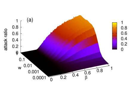
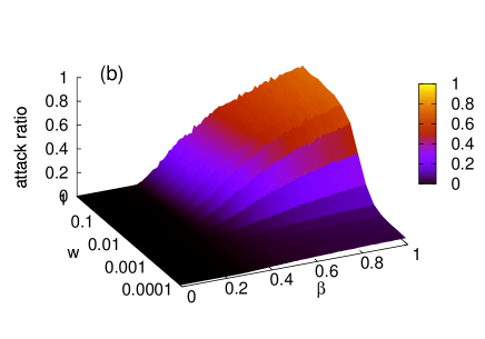
We perform numerical simulations with two different methods. The first one is the Monte Carlo method. One Monte Carlo step consists of transmission and traveling processes. In the case of the SIR model, in the -th patch, a susceptible individual becomes infected with probability , where is the time scale, and each infected individual recovers with probability [6]. In the SHIR model, a susceptible individual becomes infected with probability , an infected individual turns seriously ill with probability , and a seriously-ill individual recovers with probability . Each individual who can travel, moves from one patch with degree to another neighboring patch with probability . In Monte Carlo simulations, , , , and are treated as integers. In one Monte Carlo step, in which the time scale is taken as , the transmission process is followed by the traveling process. States of the individuals are updated after each process. Simulation continues as long as for the SIR model and for the SHIR model. The final size distributions for the metapopulation SIR and SHIR models are shown in Figs. 1(a) and 1(b), respectively. In both the distributions, the attack ratio starts to increase near , which corresponds to the epidemic threshold of . When the mobility rate is small, the attack ratio is also small in both Figs. 1(a) and 1(b).


The second numerical method involves solving the reaction-diffusion equations (1) and (2) numerically. We employ the 4th Runge-Kutta method for time evolution. In this method, , , , and are treated as real numbers. In Ref. [8], termination conditions, which are conditions to stop a simulation, were for the SIR model and for the SHIR model. Figures 2(a) and 2(b) show the final size distributions under these termination conditions for the metapopulation SIR and SHIR models, respectively. In Fig. 2(a), we see a continuous transition at (). However, in Fig. 2(b), a discontinuous jump appears at . Another important point is that the final size distributions are not related to the mobility rate . These results are almost the same as the ones reported in Ref. [8].
The reason why the final size distribution is independent of is owing to the fact that the second method is a type of a mean-field approach in which the network structure is irrelevant. In other words, the entire metapopulation network can be regarded as a large single population in the mean-field approach. In such a case, attack ratio does not depend on the mobility rate, although the time scales for the epidemic to spread and cease depend on the mobility rate. By contrast, in Monte Carlo simulations, the final size distributions are strongly dependent on the mobility rate. Furthermore, in this case, the network structure is relevant as well. When the mobility rate is very small, the epidemic cannot spread to other patches even if the transmission rate is large, although a local outbreak may occur. Since a large fraction of patches stay uninfected for a small mobility rate, the attack ratio is small even for a large transmission rate.
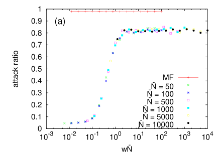
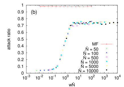
Moreover, in Monte Carlo simulations, the attack ratio depends not only on the mobility rate but also on the average population of a patch. The quantity that defines the global invasion threshold is proportional to , and depends on the network structure and other parameters [6]. In Fig. 3, the attack ratio is plotted as a function of for . For different values of , the attack ratio simulated with the Monte Carlo method collapses into a single curve. The attack ratio increases rapidly at around and saturates to a certain value. The saturated value of attack ratio in the Monte Carlo simulations is approximately –, while that in the mean-field approach is almost . This is because infected individuals disappear at some probability before the epidemic grows. This type of behavior is often observed when the initial condition has only one infected individual in the entire metapopulation.
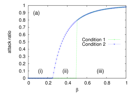
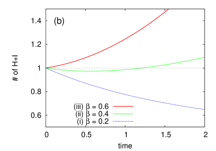
Here, we explain the reason for the discontinuous jump in the reaction-diffusion system. The key is the termination condition. When the termination threshold is almost zero, the discontinuous jump disappears. The final size distributions under different termination conditions are shown in Fig. 4(a), where the mobility rate is fixed at . The green curve in Fig. 4(a) is the same as the final size distribution in Fig. 2(b). The blue curve in Fig. 4(a) is calculated under the termination condition (more precisely, with ). It has a continuous transition at , which corresponds to . To understand the effects of different termination conditions, we separate the interval of into three regimes: (i) , (ii) , and (iii) . In Regime (i), the number of infected individuals decreases monotonically as shown in Fig. 4(b). Since is lower than the epidemic threshold, a disease cannot spread at all. By contrast, in Regime (iii), initially, the number of infected individuals increases rapidly. In these two regimes, termination conditions have no influence on the attack ratio. However, in Regime (ii), the situation is a bit complicated. The number of infected individuals decreases at first but increases after a short interval of time. This initial decay in is natural, since
| (4) |
with and at . Since in Regime (ii), the simulation stops immediately when the termination threshold is . When the threshold is closer to 0 (or ), the simulation continues, and the number of infected individuals grows enough since . In the SIR model, is equivalent to . Thus, Regime (ii) does not exist in the SIR model.
4 Conclusions
We introduced a modified metapopulation SIR model with a latent period, which we call the SHIR model, and compared the final size distributions of the metapopulation SIR and SHIR models. In Monte Carlo simulations, the distributions of both the models appear similar and depend on the mobility rate as well as the transmission rate. However, those in the reaction-diffusion systems are independent of the mobility rate and have different properties between the SIR and SHIR model. The difference between the two methods arises from the treatment of population; population is treated as an integer in Monte Carlo simulations and a real number in reaction-diffusion systems. Although the final size distribution of the SIR model has a continuous transition, that of the SHIR model shows a discontinuous jump, depending on the termination condition of the simulation. The difference caused by the termination condition indicates that a temporal decay of the number of infected individuals can mislead us into underestimating the final size of an epidemic.
References
- [1] R.M. Anderson, and R.M. May, Infectious diseases of humans: dynamics and control (Oxford University Press, Oxford, 1991).
- [2] J. Ma and D.J.D. Earn, Bull. Math. Biol. 68 (2006) 679.
- [3] R.M. May and A.L. Lloyd, Phys. Rev. E 64 (2001) 066112.
- [4] M.J. Keeling and P. Rohani, Ecol. Lett. 5 (2002) 20.
- [5] P.C. Cross, J.O. Lloyd-Smith, P.L.F. Johnson, and W.M. Getz, Ecol. Lett. 8 (2005) 587.
- [6] V. Colizza and A. Vespignani, Phys. Rev. Lett. 99 (2007) 148701.
- [7] V. Colizza and A. Vespignani, J. Theor. Biol. 251 (2008) 450.
- [8] K. Mizuno and K. Kudo, in Proceedings of the International Conference on Social Modeling and Simulation, plus Econophysics Colloquium 2014, ed. H. Takayasu, N. Ito, I. Noda and M. Takayasu (Springer Proceedings in Complexity, Springer, 2015) p. 141.
- [9] I. Schwartz and H. Smith, J. Math. Biol. 18 (1983) 233.
- [10] J.M. Hyman, J. Li, and E.A. Stanley, Math. Biosci. 155 (1999) 77.