Shifted equivalent sources and FFT acceleration for periodic scattering problems, including Wood anomalies

Abstract

This paper introduces a fast algorithm, applicable throughout the electromagnetic spectrum, for the numerical solution of problems of scattering by periodic surfaces in two-dimensional space. The proposed algorithm remains highly accurate and efficient for challenging configurations including randomly rough surfaces, deep corrugations, large periods, near grazing incidences, and, importantly, Wood-anomaly resonant frequencies. The proposed approach is based on use of certain “shifted equivalent sources” which enable FFT acceleration of a Wood-anomaly-capable quasi-periodic Green function introduced recently (Bruno and Delourme, Jour. Computat. Phys., 262–290, 2014). The Green-function strategy additionally incorporates an exponentially convergent shifted version of the classical spectral series for the Green function. While the computing-cost asymptotics depend on the asymptotic configuration assumed, the computing costs rise at most linearly with the size of the problem for a number of important rough-surface cases we consider. In practice, single-core runs in computing times ranging from a fraction of a second to a few seconds suffice for the proposed algorithm to produce highly-accurate solutions in some of the most challenging contexts arising in applications.

1 Introduction

The problem of scattering by rough surfaces has received considerable attention over the last few decades in view of its significant importance from scientific and engineering viewpoints. Unfortunately, however, the numerical solution of such problems has generally remained quite challenging. For example, the evaluation of rough-surface scattering at grazing angles has continued to pose severe difficulties, as do high-frequency problems including deep corrugations and/or large periods, and problems at certain “Wood-anomaly” frequencies. (As mentioned in Remarks 1 and 2 below, at Wood frequencies the classical quasi-periodic Green Function ceases to exist, and associated Green-function summation methods such as [22, 12, 2] become inapplicable.) In spite of significant progress in the general area of scattering by periodic surfaces [15, 1, 6, 3, 23, 11, 4], methodologies which effectively address the various aforementioned difficulties for realistic configurations have remained elusive. The present contribution proposes a new fast and accurate integral-equation methodology which addresses these challenges in the two-dimensional case. The method proceeds by introducing the notion of “shifted equivalent sources”, which extends the applicability of the FFT-based acceleration approach [7] to the context of the Wood-anomaly capable two- and three-dimensional shifted Green functions [4, 11, 5]. In the present two-dimensional case, single-core runs in computing times ranging from a fraction of a second to a few seconds suffice for the proposed algorithm to produce highly-accurate solutions in some of the most challenging contexts arising in applications—even at grazing angles and Wood frequencies. The algorithm is additionally demonstrated for certain extreme geometries featuring several hundred wavelengths in period and/or depth, for which accurate solutions are obtained in single-core runs of the order of a few minutes.

The Wood-anomaly problem has historically presented significant difficulties. In fact, the well-known challenges that arise as incidences approach grazing [13, 18, 29] are closely related to the appearance of associated near Wood anomalies (Section 6.4). As indicated in the present paper’s Remark 3, further, Wood anomalies are specially pervasive in three-dimensional configurations, and they have therefore significantly curtailed solution of periodic scattering problems in that higher-dimensional context. The extension [11] of the shifted Green function approach to three-dimensions gave rise, for the first time, to solvers which are applicable to doubly periodic scattering problems under Wood-frequencies in three-dimensional space. (An alternative approach to the Wood anomaly problem for two-dimensions was introduced in [3], but the three-dimensional, bi-periodic version [23] of that approach is restricted to frequencies away from Wood anomalies.) The contribution [11] does not include an acceleration procedure, and it can therefore prove exceedingly expensive—except when applied to relatively simple configurations. The present paper introduces, in the two-dimensional context, an accelerated version of the shifted Green-function approach. An extension of this methodology to the three-dimensional case, which will be presented elsewhere, has been found equally effective.

With reference to the nomenclature and concepts introduced in [7], in the proposed approach, a “small” number of free-space equivalent-source densities are initially computed. Subsequent convolution of those sources with the shifted quasi-periodic Green function [4, 11, 5] produces, after necessary near-field corrections, the desired quasi-periodic fields. Importantly, the near-field corrections needed in the present context are designed to account for near-field sources inherent in the shifting strategy (Section 5). Additionally, the proposed approach requires evaluation of a significantly reduced number of quasi-periodic Green function values, as low as $O(N)$, depending on the acceleration setup, instead of the $\mathcal{O}(N^{2})$ that are generally required—thus providing highly significant additional acceleration. The Green-function strategy is supplemented, finally, by an exponentially convergent shifted version of the classical spectral series for the Green function, that is used for large portions of the Cartesian acceleration grid. Use of specialized high order Nyström quadrature rules, together with the iterative linear algebra solver GMRES [28], complete the proposed methodology.

This paper is organized as follows: after a few preliminaries are laid down in Section 2, Section 3 describes the shifted Green function method [4, 11, 5], and it introduces a hybrid spatial-spectral strategy for the efficient evaluation of the shifted Green function itself. Our high order quadrature rules and their use of the hybrid evaluation strategy are put forth in Section 4. Section 5 then introduces the central concepts of this paper, namely, the shifted equivalent source method and the associated FFT acceleration approach; Section 5.7 presents an algorithmic description of the overall accelerated solution method. Section 6 demonstrates the new solver by means of a wide variety of applications. After a few concluding remarks presented in Section 7, theoretical questions concerning the convergence of the proposed algorithm are taken up briefly in Appendix A.

2 Preliminaries

We consider the problem of scattering of a transverse electric incident electromagnetic wave of the form $u^{inc}(x,y)=e^{\mathrm{i}(\alpha x-\beta y)}$ by a perfectly conducting periodic surface $\Gamma=\{\left(x,f(x)\right),x\in\mathbb{R}\}$ in two-dimensional space, where $f$ is a smooth periodic function of period $d$: $f(x+d)=f(x)$; the transverse magnetic case can be treated analogously [4]. Letting $\mathrm{k}^{2}=\alpha^{2}+\beta^{2}$, the scattered field $u^{s}$ satisfies

$$\left\{\begin{array}[]{rlc}\Delta u^{s}+\mathrm{k}^{2}u^{s}&=0&\quad\mbox{in}\quad\Omega^{+}_{f}\\ u^{s}&=-u^{inc}&\quad\mbox{in}\quad\Gamma,\end{array}\right.$$ (1)

where $\Omega^{+}_{f}=\{(x,y):y>f(x)\}$. The incidence angle $\theta\in(-\frac{\pi}{2},\frac{\pi}{2})$ is defined by $\alpha=\mathrm{k}\sin(\theta)$ and $\beta=\mathrm{k}\cos(\theta)$. As is known [24], the scattered field $u^{s}$ is quasi-periodic ($u^{s}(x+d,y)=u^{s}(x,y)e^{\mathrm{i}\alpha d}$) and, for all $(x,y)$ such that $y>\max_{x\in\mathbf{r}}f(x)$, it can be expressed in terms of a Rayleigh expansion of the form

$$u^{s}(x,y)=\sum_{n=-\infty}^{\infty}B_{n}e^{\mathrm{i}\alpha_{n}x+\mathrm{i}\beta_{n}y}.$$ (2)

Here, $B_{n}\in\mathbb{C}$ are the Rayleigh coefficients, and, letting $U$ denote the finite set of integers $n$ such that $\mathrm{k}^{2}-\alpha_{n}^{2}>0$, the wavenumbers $(\alpha_{n},\beta_{n})$ are given by

$$\alpha_{n}:=\alpha+n\frac{2\pi}{d},\hskip 30.0pt\beta_{n}:=\left\{\begin{array}[]{ccc}\sqrt{\mathrm{k}^{2}-\alpha_{n}^{2}}&,&n\in U\\ \mathrm{i}\sqrt{\alpha_{n}^{2}-\mathrm{k}^{2}}&,&n\not\in U,\\ \end{array}\right.$$ (3)

where the positive branch of the square root is used.

For $n\in U$, the functions $e^{\mathrm{i}\alpha_{n}x+\mathrm{i}\beta_{n}y}$ correspond to propagative waves. A wavenumber $\mathrm{k}$ is called a Wood-Rayleigh frequency (or, for conciseness, a Wood frequency) if for some $n\in\mathbb{Z}$ we have $\mathrm{k}^{2}=\alpha_{n}^{2}$, or equivalently, $\beta_{n}=0$. At a Wood Frequency, the function $e^{\mathrm{i}\alpha_{n}x+\mathrm{i}\beta_{n}y}=e^{\mathrm{i}\alpha_{n}x}$ becomes a grazing plane wave—that is to say, under the present conventions, a wave that propagates parallel to the $x$-axis. Note that at grazing incidence ($\theta=\frac{\pi}{2}$) we have $\alpha=\mathrm{k}$ and, thus, $\beta_{0}=0$—that is, any frequency $\mathrm{k}$ becomes a Wood anomaly at grazing incidence.

Remark 1.

The term “Wood-anomaly” relates to experimental observations by Wood [31] and a subsequent mathematical treatment by Rayleigh [27] concerning conversion of propagative to evanescent waves as frequencies or incidence angles are changed. As pointed out in [25], it would be more appropriate to refer to this phenomenon as Wood-Rayleigh anomalies and frequencies, but, throughout this paper, we use the Wood anomaly nomenclature in keeping with common practice [26, 30, 3]. A brief discussion of historical aspects concerning this terminology can be found in [4, Remark 2.2].

For $n\in U$, the $n$-th order efficiency, which is defined by $e_{n}=\frac{\beta_{n}}{\beta}|B_{n}|^{2}$, represents the fraction of the incident energy that is reflected in the $n$-th propagative mode. In particular, as is well known [24], for a perfectly conducting surface the (finitely many) efficiencies $e_{n}$ satisfy the energy balance criterion: $\sum_{n\in U}e_{n}=1$. Since integral equation methods do not enforce this relation exactly, the numerical “energy-balance” error

$$\varepsilon=1-\sum_{n\in U}e_{n},$$ (4)

is commonly used to evaluate the precision of numerical solutions. When supplemented by checks based on convergence studies as resolutions are increased, the resulting energy-balance error criterion can be very useful and reliable.

Calling

$$G(X,Y)=\frac{\mathrm{i}}{4}H_{0}^{1}(\mathrm{k}\sqrt{X^{2}+Y^{2}}),$$ (5)

the free-space Green function for the Helmholtz operator $\Delta+\mathrm{k}^{2}$ (where $H_{0}^{(1)}$ denotes the first Hankel function of order zero), the classical quasi-periodic Green function for the problem (1) is given by

$$G^{q}(X,Y)=\sum_{n\in\mathbf{Z}}e^{\mathrm{i}\alpha nd}G(X+nd,Y).$$ (6)

The Green function (6) also admits the Rayleigh representation

$$G^{\textit{qper}}(X,Y)=\frac{\mathrm{i}}{2d}\sum_{n\in\mathcal{Z}}\frac{e^{\mathrm{i}\alpha_{n}X+\mathrm{i}\beta_{n}|Y|}}{\beta_{n}},$$ (7)

a suitable modification of which can be exploited, as shown in Section 3.2, to significantly accelerate the Wood-frequency capable shifted Green function introduced in Section 3.

Remark 2.

It is important to note that at Wood frequencies the grazing wave $e^{\mathrm{i}\alpha_{n}X}$ in (7) ($\beta_{n}=0$) acquires an infinite coefficient. Accordingly [9], at Wood frequencies the lattice sum (6) blows up. The shifting strategy introduced in Section 3 gives rise to quasi-periodic Green functions which do not suffer from these difficulties.

Remark 3.

Wood frequencies (and, thus also “near-Wood frequencies”) are particularly ubiquitous in the 3D case. Indeed, while in two dimensions the proximity to a Wood frequency configuration is characterized by the closest distance from $\mathrm{k}^{2}$ to the discrete lattice $\alpha_{n}^{2}$, that is, by the quantity

$$R_{\mathrm{wood}}=\min_{n\in\mathbf{Z}}\beta_{n}=\min\left\{\sqrt{\mathrm{k}^{2}-\left(\alpha+2\pi n/d\right)^{2}}:n\in\mathbf{Z}\right\},$$ (8)

the corresponding expression for the 3D case (for incidence wavevector $(\alpha_{1},\alpha_{2},-\beta)$) is given by

$$R_{\mathrm{wood}}=\min\left\{\sqrt{\mathrm{k}^{2}-\left(\alpha_{1}+2\pi n/d_{1}\right)^{2}-\left(\alpha_{2}+2\pi m/d_{2}\right)^{2}}:(n,m)\in\mathbf{Z}^{2}\right\}.$$ (9)

Therefore, in 3D, near Wood frequencies arise for all points in the lattice $(\alpha_{1},\alpha_{2})+\left(\frac{2\pi}{d_{1}}\mathbf{Z}\right)\times\left(\frac{2\pi}{d_{2}}\mathbf{Z}\right)$ that lie on circles of radii close to $\mathrm{k}$ and are thus quite numerous for large values of $\mathrm{k}$: for a given arbitrarily small distance $\varepsilon$, in the 3D case there are $O(\mathrm{k})$ such frequencies within an $\varepsilon$ band around the circle of radius $\mathrm{k}$ in the plane. For sufficiently small $\varepsilon$ the corresponding number in the 2D case is at most two.

3 Shifted Green function

As shown in [4, 11], a suitable modification of the Green function (7) which does not suffer from the difficulties mentioned in Remark 2, and which is therefore valid throughout the spectrum, can be introduced on the basis of a certain “shifting” procedure related to the method of images. In what follows, the construction [4] of a multipolar or “shifted” quasi-periodic Green function is reviewed briefly, and a new hybrid spatial-spectral strategy for its evaluation is presented.

3.1 Quasi-periodic multipolar Green functions

Rapidly decaying multipolar Green functions $G_{j}$ of various orders $j$ can be obtained as linear combinations of the regular free-space Green function $G$ with arguments that include a number $j$ of shifts. For example, we define a multipolar Green function of order $j=1$ by

$$G_{1}(X,Y)=G(X,Y)-G(X,Y+h)$$ (10)

This expression provides a Green function for the Helmholtz equation, valid in the complement of the shifted-pole set $P_{1}=\{(0,-h)\}$, which decays faster than $G$ (with order $|X|^{-\frac{3}{2}}$ instead of $|X|^{-\frac{1}{2}}$) as $X\to\infty$—as there results from a simple application of the mean value theorem and the asymptotic properties of Hankel functions [21].

A suitable generalization of this idea, leading to multipolar Green functions with arbitrarily fast algebraic decay [4], results from application of the finite-difference operator $(u_{0},\dots,u_{j})\to\sum_{\ell=0}^{j}(-1)^{\ell}\binom{j}{\ell}u_{\ell}$ ($j\in\mathbb{N}$) that, up to a factor of $1/h^{j}$, approximates the $j$-th order $Y$-derivative operator [20, eq. 5.42]. For each non-negative integer $j$, the resulting multipolar Green functions $G_{j}$ of order $j$ is thus given by

$$G_{j}(X,Y)=\sum_{m=0}^{j}(-1)^{m}C_{m}^{j}\,G(X,Y+mh),\quad\mbox{where}\quad C_{m}^{j}=\binom{j}{m}=\frac{j!}{m!(j-m)!}.$$ (11)

Clearly, $G_{j}$ is a Green function for the Helmholtz equation in the complement of the shifted-pole set

$$P_{j}=\{(X,Y)\in\mathbb{R}^{2}:(X,Y)=(0,-mh)\mbox{ for some }m\in\mathbb{Z}\mbox{ with }1\leq m\leq j\}.$$ (12)

As shown in [4], further, for $Y$ bounded we have

$$G_{j}(X,Y)\sim|X|^{-q}\mbox{ as }X\to\infty,\quad\mbox{with}\quad q=\frac{1}{2}+\left\lfloor{\frac{j+1}{2}}\right\rfloor,$$ (13)

where $\left\lfloor{x}\right\rfloor$ denotes the largest integer less than or equal to $x$.

For sufficiently large values of $j$, the spatial lattice sum

$$\tilde{G}_{j}^{\textit{qper}}(X,Y)=\sum_{n=-\infty}^{\infty}e^{-\mathrm{i}\alpha nd}G_{j}(X+nd,Y)$$ (14)

provides a rapidly (algebraically) convergent quasi-periodic Green function series defined for all $(X,Y)$ outside the periodic shifted-pole lattice

$$P_{j}^{\textit{qper}}=\{(X,Y)\in\mathbb{R}^{2}:(X,Y)=(nd,-mh)\mbox{ for some }n,m\in\mathbb{Z}\mbox{ with }1\leq m\leq j\}.$$ (15)

The Rayleigh expansion of $\tilde{G}_{j}^{\textit{qper}}$, further, can be readily obtained by applying equation (7); the result is

$$\tilde{G}_{j}^{\textit{qper}}(X,Y)=\sum_{n=-\infty}^{\infty}\frac{\mathrm{i}}{2d\beta_{n}}e^{\mathrm{i}\alpha_{n}X}\left(\sum_{m=0}^{j}(-1)^{m}C_{m}^{j}e^{\mathrm{i}\beta_{n}|Y+mh|}\right)\qquad\mbox{for }Y\not=-mh,\quad 0\leq m\leq j.$$ (16)

And, using the identity $\sum_{m=0}^{j}(-1)^{m}C_{m}^{j}e^{\mathrm{i}\beta_{n}(Y+mh)}=e^{\mathrm{i}\beta_{n}Y}(1-e^{\mathrm{i}\beta_{n}h})^{j}$ there results

$$\tilde{G}_{j}^{\textit{qper}}(X,Y)=\sum_{n=-\infty}^{\infty}\frac{\mathrm{i}}{2d\beta_{n}}(1-e^{\mathrm{i}\beta_{n}h})^{j}e^{\mathrm{i}\alpha_{n}X+\mathrm{i}\beta_{n}Y}\qquad\mbox{for }Y>0.$$ (17)

As anticipated, no problematic infinities occur in the Rayleigh expansion of $\tilde{G}_{j}^{\textit{qper}}$, even at Wood anomalies ($\beta_{n}=0$), for any $j\geq 1$. The shifting procedure has thus resulted in rapidly-convergent spatial representations of various orders (equations (13) and (14)) as well as spectral representations which do not contain infinities (equation (17)).

An issue does arise from the shifting method which requires attention: the shifting procedure cancels certain Rayleigh modes for $Y>0$ and thereby affects the ability of the Green function to represent general fields. In detail, the coefficient $(1-e^{\mathrm{i}\beta_{n}h})^{j}\beta_{n}^{-1}$ in the series (17) vanishes if either $\beta_{n}=0$ (Wood anomaly) and $j\geq 1$, or if $\beta_{n}h$ equals an integer multiple of $2\pi$. As in [4], we address this difficulty by simply adding to $\tilde{G}_{j}^{\textit{qper}}$ the missing modes. In fact, in a numerical implementation it is beneficial to incorporate corrections containing not only resonant modes, but also nearly resonant modes. Thus, using a sufficiently small number $\eta$ and defining the $\eta$-dependent completion function

$$M^{\eta}(X,Y)=\sum_{n\in U^{\eta}}e^{\mathrm{i}\alpha_{n}X+\mathrm{i}\beta_{n}Y},\qquad U^{\eta}=\left\{n\in\mathbb{Z}:|(1-e^{\mathrm{i}\beta_{n}h})^{j}\beta_{n}^{-1}|<\eta\right\},$$ (18)

(where for $\beta_{n}=0$ the quotient $|(1-e^{\mathrm{i}\beta_{n}h})^{j}\beta_{n}^{-1}|$ is interpreted as the corresponding limit as $\beta_{n}\to 0$), a complete version of the shifted Green function is given by

$$G_{j}^{\textit{qper}}(X,Y)=\tilde{G}_{j}^{\textit{qper}}(X,Y)+M^{\eta}(X,Y)$$ (19)

for $(X,Y)$ outside the set $P_{j}^{\textit{qper}}$.

Remark 4.

The following section presents an algorithm which, relying on both equations (14) and (16), rapidly evaluates the Green function $\tilde{G}_{j}^{\textit{qper}}$. Section 4 presents integral equation formulations based on separate use of the functions $\tilde{G}_{j}^{\textit{qper}}$ and $M^{\eta}$, that avoids a minor difficulty (addressed in [4, Remark 4.8]) related to the direct use of the Green function $G_{j}^{\textit{qper}}$ defined in (19).

3.2 Hybrid spatial-spectral evaluation of $\tilde{G}_{j}^{\textit{qper}}$

Equation (17) provides a very useful expression for evaluation of $\tilde{G}_{j}^{\textit{qper}}$ for $Y>0$ at all frequencies, including Wood anomalies—since, for such values of $Y$, this series converges exponentially fast. Interestingly, further, the related expression (16) can also be used, again, with exponentially fast convergence, including Wood anomalies, for all values of $Y$ sufficiently far from the set $\{Y=-mh:\;0\leq m\leq j\}$. The latter expression thus provides a greatly advantageous alternative to direct summation of the series (14) for a majority (but not not the totality) of points $(X,Y)$ relevant in a given quasi-periodic scattering problem.

The exponential convergence of (16) is clear by inspection. To see that (16) is well defined at and around Wood anomalies it suffices to substitute the sum in $m$ in equation (16) by the expression

$$\sum_{m=0}^{j}(-1)^{m}C_{m}^{j}\frac{e^{\mathrm{i}\beta_{n}|Y+mh|}}{\beta_{n}}=e^{\mathrm{i}\beta_{n}Y}\frac{(1-e^{\mathrm{i}\beta_{n}h})^{j}}{\beta_{n}}-\sum_{\begin{subarray}{c}0\leq m\leq j\\ m<-Y/h\end{subarray}}(-1)^{m}C_{m}^{j}\frac{e^{\mathrm{i}\beta_{n}(Y+mh)}-e^{-\mathrm{i}\beta_{n}(Y+mh)}}{\beta_{n}}.$$ (20)

where, once again, the values of the quotients containing $\beta_{n}$ denominators at $\beta_{n}=0$ are interpreted as the corresponding $\beta_{n}\to 0$ limits.

A strategy guiding the selection of the values $Y$ for which the spectral series (16) is used instead of the spatial series (14) can be devised on the basis of the relation

$$\beta_{n}=\mathrm{k}\sqrt{1-(\sin(\theta)+\frac{\lambda}{d}n)^{2}}\;\approx\;\mathrm{\mathrm{i}}\mathrm{k}\frac{\lambda}{d}n+\mathcal{O}(1)\;=\;\frac{2n\pi}{d}\mathrm{i}+\mathcal{O}(1).$$ (21)

Indeed, the estimate

$$\left|e^{\mathrm{i}\beta_{n}|Y+mh|}\right|<Ce^{-2n\pi\frac{\delta}{d}},\quad(|Y+mh|>\delta>0)$$ (22)

shows that, for $|Y+mh|>\delta>0$, the spectral representation (16) converges like a geometric series of ratio $e^{-2\pi\frac{\delta}{d}}<1$—with fast convergence for values of $\frac{\delta}{d}$ sufficiently far from zero.

4 Hybrid, high-order Nyström solver throughout the spectrum

4.1 Integral equation formulation

The Green functions $G_{j}^{\textit{qper}}$ presented in Section 3 (equation (19)) can be used to devise an integral equation formulation for problem (1) which remains valid at Wood Anomalies [4]. As indicated in Remark 4, however, we proceed in a slightly different manner. Letting $\nu(x^{\prime})$ denote the normal to the curve $\Gamma$ at the point $(x^{\prime},f(x^{\prime}))$ and $ds^{\prime}$ denote the element of length on $\Gamma$ at $(x^{\prime},f(x^{\prime}))$, we express the scattered field $u^{scat}$ in (1), for all $(x,y)\in\Omega^{+}_{f}$, as a multipolar double layer potential plus a potential with kernel $M^{\eta}$:

$$u^{scat}(x,y)=\int_{0}^{d}\left(\nu(x^{\prime})\cdot\nabla_{(x^{\prime},y^{\prime})}\tilde{G}_{j}^{\textit{qper}}(x-x^{\prime},y-y^{\prime})\big{|}_{y^{\prime}=f(x^{\prime})}+M^{\eta}(x-x^{\prime},y-f(x^{\prime}))\right)\mu(x^{\prime})ds^{\prime}.$$ (23)

Defining the normal-derivative operator $\partial_{\nu^{\prime}}$, whose action on a given function $K:\mathbb{R}\times\mathbb{R}\to\mathbb{C}$ is given by

$$\partial_{\nu^{\prime}}K(x,x^{\prime})=\left[\nu(x^{\prime})\cdot\nabla_{(x^{\prime},y^{\prime})}K(x-x^{\prime},y-y^{\prime})\right]_{y=f(x),y^{\prime}=f(x^{\prime})},$$ (24)

and, letting $D$ denote the integral operator

$$D[\mu](x)=\int_{0}^{d}\left(\partial_{\nu^{\prime}}\tilde{G}_{j}^{\textit{qper}}(x,x^{\prime})+M^{\eta}(x-x^{\prime},f(x)-f(x^{\prime}))\right)\mu(x^{\prime})ds^{\prime},\quad x\in[0,d],$$ (25)

it follows that $\mu$ satisfies the integral equation

$$\frac{1}{2}\mu(x)+D[\mu](x)=-u^{inc}(x)\quad\mbox{for}\quad x\in[0,d].$$ (26)

We may also write

$$D[\mu]=\tilde{D}[\mu]+D_{M}[\mu]$$ (27)

where

$$\tilde{D}[\mu](x)= \int_{0}^{d}\partial_{\nu^{\prime}}\tilde{G}_{j}^{\textit{qper}}(x,x^{\prime})\mu(x^{\prime})ds^{\prime}\quad\mbox{and}$$ (28)

$$D_{M}[\mu](x)= \int_{0}^{d}M^{\eta}(x-x^{\prime},f(x)-f(x^{\prime}))\mu(x^{\prime})ds^{\prime}.$$ (29)

It is easy to check [4], finally, that the operator $\tilde{D}$ can be expressed as the infinite integral

$$\tilde{D}[\mu](x)=\int_{-\infty}^{+\infty}\partial_{\nu^{\prime}}G_{j}(x,x^{\prime})\mu(x^{\prime})ds_{\Gamma}(x^{\prime}),$$ (30)

where $\mu$ is extended to all of $\mathbb{R}$ by $\alpha$-quasi-periodicity:

$$\mu(x+d)=\mu(x)e^{\mathrm{i}\alpha d}.$$ (31)

The proposed fast iterative Nyström solver for equation (26) is based on use of an equispaced discretization of the periodicity interval $[0,d]$, an associated quadrature rule, and an FFT-based acceleration method. The underlying high-order quadrature rule, which is closely related to the one used in [4, Sect. 5], but which incorporates a highly-efficient hybrid spatial-spectral approach for the evaluation of the Green function, is detailed in Section 4.2. On the basis of this quadrature rule alone, an unaccelerated Nyström solver for equation (26) is presented in Section 4.3; a discussion concerning the convergence of this algorithm is put forth in Appendix A. The proposed acceleration technique and resulting overall accelerated solver are presented in Section 5.

4.2 High-order quadrature for the incomplete operator $\tilde{D}$

In the proposed Nyström approach, the smooth windowing function

$$S_{\gamma,a}(x)=\left\{\begin{array}[]{ccc}1&\text{if }|x|\leq\gamma,&\\ \exp\left(\frac{2e^{-1/u}}{u-1}\right)&\text{if }\gamma<|x|<a,&u=\frac{|x|-\gamma}{a-\gamma},\\ 0&\text{if }|x|\geq a,&\\ \end{array}\right.$$ (32)

(see Figure 1) is used to decompose the operator $\tilde{D}$ in equation (30) as a sum $\tilde{D}=\tilde{D}_{\mathrm{reg}}+\tilde{D}_{\mathrm{sing}}$ of regular and singular contributions $\tilde{D}_{\mathrm{reg}}$ and $\tilde{D}_{\mathrm{sing}}$, given by

$$\tilde{D}_{\mathrm{reg}}[\mu](x)=\int_{-\infty}^{+\infty}\partial_{\nu^{\prime}}G_{j}(x,x^{\prime})(1-S_{\gamma,a}^{f}(x,x^{\prime}))\mu(x^{\prime})ds^{\prime}$$ (33)

and

$$\tilde{D}_{\mathrm{sing}}[\mu](x)=\int_{x-a}^{x+a}\partial_{\nu^{\prime}}G_{j}(x,x^{\prime})S_{\gamma,a}^{f}(x,x^{\prime})\mu(x^{\prime})ds^{\prime}.$$ (34)

where we have defined

$$S_{\gamma,a}^{f}(x,x^{\prime})=S_{\gamma,a}\left(\sqrt{(x-x^{\prime})^{2}+(f(x)-f(x^{\prime}))^{2}}\right).$$ (35)

Remark 5.

The parameter $a$ is selected so as to appropriately isolate the logarithmic singularity. For definiteness, throughout this chapter it is assumed the relation $a<d$ is satisfied.

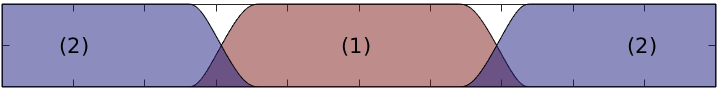
Figure 1: Partition of Unity functions $S_{\gamma,a}(x)$ and $1-S_{\gamma,a}(x)$, labeled (1) and (2), respectively.

To derive quadrature rules for the operators $\tilde{D}_{\mathrm{reg}}$ and $\tilde{D}_{\mathrm{sing}}$ we consider an equispaced discretization mesh $\{x_{\ell}\}_{\ell=-\infty}^{\infty}$, of mesh-size $\Delta x=(x_{\ell+1}-x_{\ell})$, for the complete real line, which is additionally assumed to satisfy $x_{0}=0$ and $x_{N}=d$ for a certain integer $N>0$. The corresponding numerical approximations of the values $\mu(x_{\ell})$ ($1\leq\ell\leq N$) will be denoted by $\mu_{\ell}$; in view of (31) the quantities $\mu_{\ell}$ are extended to all $\ell\in\mathbb{Z}$ by quasi-periodicity:

$$\mu_{(\ell+pN)}=\mu_{\ell}\ e^{\mathrm{i}\alpha pd}\qquad\ell=1,\dots,N\quad p\in\mathbb{Z}.$$ (36)

4.2.1 Discretization of the operator $\tilde{D}_{\mathrm{sing}}$

To discretize the operator $\tilde{D}_{\mathrm{sing}}$ we employ the Martensen-Kussmaul (MK) splitting [14] of the Hankel function $H_{1}^{1}$ into logarithmic and smooth contributions. Following [4, Secs. 5.1-5.2] we thus obtain the decomposition

$$\partial_{\nu^{\prime}}G_{j}(x,x^{\prime})=K_{s}(x,x^{\prime})\ln\left[4\sin^{2}\left(\frac{\pi}{a}(x-x^{\prime})\right)\right]+K_{r}(x,x^{\prime})$$ (37)

where the smooth kernels $K_{s}$ and $K_{r}$ are given by

$$K_{s}(x,x^{\prime})=\frac{\mathrm{k}}{4\pi}\frac{f(x^{\prime})(x-x^{\prime})-(f(x^{\prime})-f(x))}{\sqrt{(x-x^{\prime})^{2}+(f(x)-f(x^{\prime}))^{2}}}J_{1}(\mathrm{k}\sqrt{(x-x^{\prime})^{2}+(f(x)-f(x^{\prime}))^{2}})$$ (38)

and

$$K_{r}(x,x^{\prime})=\partial_{\nu^{\prime}}G_{j}(x,x^{\prime})-K_{s}(x,x^{\prime})\ln\left[4\sin^{2}\left(\frac{\pi}{a}(x-x^{\prime})\right)\right].$$ (39)

Replacing (37) into (34) we obtain $\tilde{D}_{\mathrm{sing}}=\tilde{D}_{\mathrm{sing}}^{\mathrm{log}}+\tilde{D}_{\mathrm{sing}}^{\mathrm{trap}}$ where

$$\tilde{D}_{\mathrm{sing}}^{\mathrm{log}} =\int_{x-a}^{x+a}\ln\left[4\sin^{2}\left(\frac{\pi}{a}(x-x^{\prime})\right)\right]K_{s}(x,x^{\prime})S_{\gamma,a}^{f}(x,x^{\prime})\mu(x^{\prime})ds^{\prime}\quad\mbox{and}$$ (40)

$$\tilde{D}_{\mathrm{sing}}^{\mathrm{trap}} =\int_{x-a}^{x+a}K_{r}(x,x^{\prime})S_{\gamma,a}^{f}(x,x^{\prime})\mu(x^{\prime})ds^{\prime}.$$ (41)

The operator $\tilde{D}_{\mathrm{sing}}^{\mathrm{log}}$ contains the logarithmic singularity; the operator $\tilde{D}_{\mathrm{sing}}^{\mathrm{trap}}$ on the other hand, may be approximated accurately by means of the trapezoidal rule.

Given that $S_{\gamma,a}^{f}(x,x^{\prime})$ vanishes smoothly at $x^{\prime}=x\pm a$ together with all of its derivatives, we can obtain high-order quadratures for each of these integrals on the basis of the equispaced discretization $\{x_{\ell}\}$ ($\ell\in\mathbb{Z}$) and the Fourier expansions of the smooth factor $K_{s}(x,x^{\prime})S_{\gamma,a}^{f}(x,x^{\prime})\mu(x^{\prime})$. Indeed, utilizing the aforementioned discrete approximations $\mu_{\ell}$ (where $\ell$ may lie outside the range $1\leq\ell\leq N$), relying on certain explicitly-computable Fourier-based weights $R_{i\ell}$ (which can be computed for general $a$ by following the procedure used in [4, Sec. 5.2] for the particular case in which $a$ equals a half period $d/2$), and appropriately accounting for certain near-singular terms in the kernel $K_{r}$ by Fourier interpolation of $\mu(x^{\prime})S_{\gamma,a}^{f}(x,x^{\prime})$ (as detailed in [4, Sec. 5.3]), a numerical-quadrature approximation

$$\tilde{D}^{\Delta x}_{\mathrm{sing}}[\mu_{1},\dots,\mu_{N}](x_{i})=\sum_{\ell\in L_{i}^{a}}R_{i\ell}K_{s}(x_{i},x_{\ell})S_{\gamma,a}^{f}(x_{i},x_{\ell})\mu_{\ell}+\sum_{\ell\in L_{i}^{a}}W_{i\ell}K_{r}(x_{i},x_{\ell})S_{\gamma,a}^{f}(x_{i},x_{\ell})\mu_{\ell}$$ (42)

of $\tilde{D}_{\mathrm{sing}}[\mu](x_{i})$ is obtained. Here $L_{i}^{a}:\{\ell:|x_{\ell}-x_{i}|\leq a\}$, and, for values of $\ell>N$ and $\ell<1$, $\mu_{\ell}$ is given by (36).

4.2.2 Discretization of the operator $\tilde{D}_{\mathrm{reg}}$

The windowing function $S_{\gamma,a}$ (with “relatively small” values of $a$) was used in the previous section to discriminate between singular and regular contributions $\tilde{D}_{\mathrm{sing}}$ and $\tilde{D}_{\mathrm{reg}}$ to the operator $\tilde{D}$. A new windowing function $S_{cA,A}(x-x^{\prime})$ (intended for use with “large” values of $A$) is now introduced to smoothly truncate the infinite integral that defines the operator $\tilde{D}_{\mathrm{reg}}$: the truncated operator is defined by

$$\tilde{D}_{\mathrm{reg}}^{A}[\mu](x)=\int_{x-A}^{x+A}\partial_{\nu^{\prime}}G_{j}(x,x^{\prime})(1-S_{\gamma,a}^{f}(x,x^{\prime}))\mu(x^{\prime})S_{cA,A}(x-x^{\prime})ds^{\prime}.$$ (43)

Defining the windowed Green function by

$$\tilde{G}^{q,A}_{j}(X,Y)=\sum_{p=-\infty}^{\infty}G_{j}(X+dp,Y)S_{cA,A}(X+dp),$$ (44)

the truncated operator $\tilde{D}_{\mathrm{reg}}^{A}$ can also be expressed in the form

$$\tilde{D}_{\mathrm{reg}}^{A}[\mu](x)=\int_{x-d/2}^{x+d/2}\partial_{\nu^{\prime}}\tilde{G}^{q,A}_{j}(x,x^{\prime})(1-S_{\gamma,a}^{f}(x,x^{\prime}))\mu(x^{\prime})ds^{\prime}.$$ (45)

On account of the smoothness of the integrand in (43), and the fact that it vanishes identically outside $[x-A,x+A]$, the integral (43) is approximated with superalgebraic order of integration accuracy by the discrete trapezoidal rule expression

$$\tilde{D}_{\mathrm{reg}}^{A,\Delta x}[\mu_{1},\dots,\mu_{N}](x_{i})=\sum_{\ell=-\infty}^{\infty}\partial_{\nu^{\prime}}G_{j}(x_{i},x_{\ell})S_{cA,A}(x_{i}-x_{\ell})(1-S_{\gamma,a}^{f}(x_{i},x_{\ell}))\mu_{\ell}(\Delta s)_{\ell}$$ (46)

where $(\Delta s)_{\ell}$ denotes the discrete surface element $\Delta x\sqrt{1+f(x_{\ell})^{2}}$, and with $\mu_{\ell}$ replaced by $\mu(x_{\ell})$ ($\ell=1,\dots,N$); see also (31) and (36).

Remark 6.

The claimed superalgebraic integration accuracy of the right-hand expression in (46) for a fixed value of $A$ follows from the well known trapezoidal-rule integration-accuracy result for smooth periodic function integrated over their period [19])—since the restriction of the integrand to $[x-A,x+A]$ can be extended to all of $\mathbb{R}$ as a smooth and periodic function $F^{A,x}=F^{A,x}(x^{\prime})$ of period $2A$.

An analysis of the smooth truncation procedure, namely, of the convergence of $\tilde{D}_{\mathrm{reg}}^{A}$ to $\tilde{D}_{\mathrm{reg}}$ as $A\to\infty$, is easily established on the basis of the convergence analysis [4, 10, 11] for the windowed-Green-function (44) to the regular shifted series (14)

$$\tilde{G}^{\textit{qper}}_{j}(x,y)=\lim_{A\to\infty}\tilde{G}^{q,A}_{j}(x,y).$$ (47)

The overall error resulting from the combined use of smooth truncation and trapezoidal discretization is discussed in Section A. In particular, Lemma 1 in that appendix provides an error estimate that shows that the superalgebraic order of trapezoidal integration accuracy is also uniform with respect to $A$.

Clearly, the numerical method embodied in equations (42) and (46) provides a high-order strategy for the evaluation of the operator $\tilde{D}$ in equation (30). As shown in the following section, a hybrid spatial/spectral Green-function evaluation strategy can be used to significantly decrease the costs associated with evaluation of the discrete operator in equation (46). While this strategy suffices in many cases, when used in conjunction with the FFT acceleration method introduced in Section 5 a solver results which, as mentioned in the introduction, enables treatment of challenging rough-surface scattering problems.

4.2.3 Spatial/Spectral hybridization

To obtain a hybrid strategy we express (46) in terms of the function $\tilde{G}^{\textit{qper}}_{j}$ which we then evaluate by means of either (16) or (47), whichever is preferable for each pair $(x_{i},x_{\ell})$. Taking limit as $A\to\infty$ in (16) we obtain the limiting discrete operator

$$\tilde{D}_{\mathrm{reg}}^{\Delta x}[\mu_{1},\dots,\mu_{N}](x_{i})=\sum_{\ell=-\infty}^{\infty}\mu_{\ell}(1-S_{\gamma,a}^{f}(x_{i},x_{\ell}))\partial_{\nu^{\prime}}G_{j}(x_{i},x_{\ell})(\Delta s)_{\ell}.$$ (48)

Writing, for every $\ell\in\mathbb{Z}$, $x_{\ell}=x_{k}-dp$ for a unique integers $k$ and $p$ ($1\leq k\leq N$), exploiting the periodicity of the function $f$ and the $\alpha$-quasi-periodicity of $\mu$, using (44) and (47), and taking into account Remark 5, we obtain the alternative expression

$$\tilde{D}_{\mathrm{reg}}^{\Delta x}[\mu_{1},\dots,\mu_{N}](x_{i})=\sum_{m=1}^{N}\partial_{\nu^{\prime}}\tilde{G}^{\textit{qper},\star}_{j}(x_{i},x_{k})\mu_{k}(\Delta s)_{k},$$ (49)

where we have set

$$\tilde{G}^{\textit{qper},\star}_{j}(X,Y)=\tilde{G}^{\textit{qper}}_{j}(X,Y)-\sum_{p=-1}^{1}G_{j}(X+dp,Y)e^{-\mathrm{i}\alpha dp}S_{\gamma,a}(X+dp).$$ (50)

Clearly, $\tilde{G}^{\textit{qper},\star}_{j}$ is a smooth function that results from subtraction from $\tilde{G}^{\textit{qper}}_{j}(X,Y)$ of (windowed versions of) the nearest interactions (modulo the period).

The expression (49) relies, via (50), on the evaluation of the exact quasi-periodic Green function $\tilde{G}^{\textit{qper}}_{j}(X,Y)$. For a given point $(X,Y)$ this function can be evaluated by either a spectral or a spatial approach: use of the spectral series as described in Section 3.2 is preferable for values of $Y$ sufficiently far from the set $\{Y=-mh:\;0\leq m\leq j\}$, while, in view of the fast convergence [4, 10, 11] of (47), for other values of $Y$ the spatial expansion (44) with a sufficiently large value of $A$ can be more advantageous. (Note that if the grating is deep enough, then $f(x)$ could be far from $f(x^{\prime})$ even if $x$ is relatively close to $x^{\prime}$. The exponentially convergent spectral approach could provide the most efficient alternative in such cases.)

4.3 Overall discretization and (unaccelerated) solution of equation (26)

Taking into account equation (27) in conjunction with the Green function evaluation and discretization strategies presented in Section (4.2) for the operator $\tilde{D}$, a full discretization for the complete operator $D$ in (25) can now be obtained easily: an efficient discretization of the remaining operator $D_{M}$ in (29), whose kernel is given by equation (18), can be produced via a direct application of the trapezoidal rule. Separating the variables $X$ and $Y$ in the exponentials $e^{\mathrm{i}\alpha_{n}X+\mathrm{i}\beta_{n}Y}$, further, the resulting discrete operator may be expressed in the form

$$D_{M}^{\Delta x}[\mu_{1},\dots,\mu_{N}](x_{i})=\sum_{n\in U^{\eta}}e^{\mathrm{i}\alpha_{n}x_{i}}\left(\sum_{\ell=1}^{N}e^{\mathrm{i}\beta_{n}f(x_{\ell})}\mu_{\ell}(\Delta s)_{\ell}\right).$$ (51)

Letting

$$D^{\Delta x}=\tilde{D}^{\Delta x}_{\mathrm{sing}}+\tilde{D}^{\Delta x}_{\mathrm{reg}}+D^{\Delta x}_{M}$$ (52)

we thus obtain the desired discrete version

$$\left(\frac{1}{2}I+D^{\Delta x}\right)[\mu_{1},\dots,\mu_{N}](x_{i})=-u^{inc}(x_{i})$$ (53)

of equation (26).

As mentioned in Section 1, the proposed method relies on use of an iterative linear algebra solver such as GMRES [28]. The necessary evaluation of the action of the discrete operator $D^{\Delta x}$ is accomplished, in the direct (unaccelerated) implementation considered in this section, via straightforward applications of the corresponding expressions (42), (49) and (51) for the operators $\tilde{D}^{\Delta x}_{\mathrm{sing}}$, $\tilde{D}^{\Delta x}_{\mathrm{reg}}$ and $D^{\Delta x}_{M}$, respectively. This completes the proposed unaccelerated iterative solver for equation (26).

The computational cost required by the various components of this solver can be estimated as follows.

1. The application of the local operator $\tilde{D}^{\Delta x}_{\mathrm{sing}}$ requires $\mathcal{O}(N)$ arithmetic operations, the vast majority of which are those associated with evaluation of the multipolar Green function $G_{j}$.

2. $D^{\Delta x}_{M}$, in turn, requires $\mathcal{O}(N)$ operations, including the computation of a number $\mathcal{O}(N)$ of values of exponential functions.

3. The operator $\tilde{D}^{\Delta x}_{\mathrm{reg}}$, finally, requires $\mathcal{O}(N^{2})$ arithmetic operations, including the significant cost associated with the evaluation of $\mathcal{O}(N^{2})$ values of the shifted-quasi-periodic Green function $\tilde{G}^{\textit{qper}}_{j}$.

Clearly, the cost mentioned in point 3 above represents the most significant component of the cost associated of the evaluation of $D^{\Delta x}$. Thus, although highly accurate, the direct $\mathcal{O}(N^{2})$-cost strategy outlined above for the evaluation of $D^{\Delta x}$ can pose a significant computational burden for problems which, as a result of high-frequency and/or complex geometries, require use of large numbers $N$ of unknowns. A strategy is presented in the next section which, on the basis of equivalent sources and Fast Fourier transforms leads to significant reductions in the cost of the evaluation of this operator, and, therefore, in the overall cost of the solution method.

5 Shifted Equivalent-Source Acceleration

The most significant portion of the computational cost associated with the strategy described in the previous section concerns the evaluation of the discrete operator $\tilde{D}_{\mathrm{reg}}^{\Delta x}$ in equation (48). The present section introduces an acceleration method for the evaluation of that operator which, incorporating an FFT-based algorithm that is applicable throughout the spectrum, reduces very significantly the number of necessary evaluations of the periodic Green function $\tilde{G}_{j}^{\textit{qper}}$, with corresponding reductions in the cost of the overall approach. A degree of familiarity with the acceleration methodology introduced in [7] could be helpful in a first reading of this section.

Central to the contribution [7] is the introduction of “monopole and dipole” representations and an associated notion of “adjacency” that, in modified forms, are used in the present algorithm as well. In order to extend the applicability of the method [7] to the context of this paper, the present Section 5 introduces certain “shifted equivalent source” representations and a corresponding validity-ensuring notion of “adjacency”. The geometrical structure that underlies the approach as well an outline of the reminder of Section 5 are presented in Section 5.1.

5.1 Geometric setup

In order to incorporate equivalent sources, the algorithm utilizes a “reference periodicity domain” $\Omega_{\textit{per}}=[0,d)\times[h_{\mathrm{min}},h_{\mathrm{max}})$, where $h_{\mathrm{min}}$ and $h_{\mathrm{max}}$ are selected so as to satisfy $[\min(f),\max(f)]\subset[h_{\mathrm{min}},h_{\mathrm{max}}]$. The domain $\Omega_{\textit{per}}$ is subsequently partitioned in a number $n_{\mathrm{cell}}=n_{x}n_{y}$ of mutually disjoint square cells $c^{q}$—whose side $L$, we assume, satisfies

$$d=n_{x}L\qquad\mbox{and}\qquad(h_{\mathrm{max}}-h_{\mathrm{min}})=n_{y}L$$ (54)

for certain positive integers $n_{x}$ and $n_{y}$. We additionally denote by $\Omega_{\infty}=(-\infty,+\infty)\times[h_{\mathrm{min}},h_{\mathrm{max}}]$; clearly $\Omega_{\infty}$ domain that is similarly partitioned into (an infinite number of) cells $c^{q}$ ($q\in\mathbb{Z}$):

$$\Omega_{\mathrm{per}}=\bigcup_{q=1}^{n_{\mathrm{cell}}}c^{q}\qquad\mbox{and}\qquad\Omega_{\infty}=\bigcup_{q=-\infty}^{\infty}c^{q}=\bigcup_{n=-\infty}^{\infty}\Big{(}\Omega_{\mathrm{per}}+nd\Big{)}.$$ (55)

Remark 7.

It is additionally assumed that the side $L$ of the accelerator cells $c^{q}$ is selected in such a way that these cells are not resonant for the given wavenumber $\mathrm{k}$—that is to say, that $-\mathrm{k}^{2}$ is not a Dirichlet eigenvalue for the Laplace operator in the cells $c^{q}$. This is a requirement in the plane-wave Dirichlet-problem solver described in Section 5.6. Clearly, values of the parameters $L$, $h_{\mathrm{max}}$, $h_{\mathrm{min}}$, $n_{x}$ and $n_{y}$ meeting this constraint as well as (54) can be found easily. Finally, the parameter $L$ is chosen so as to minimize the overall computing cost, while meeting a prescribed accuracy tolerance. In all cases considered in this chapter values of $L$ in the range between one and four wavelengths were used.

Remark 8.

In order to avoid cell intersections, throughout this chapter the cells $c^{q}$ are assumed to include the top and right sides, but not to include the bottom and left sides. In other words, it is assumed that each cell $c^{q}$ can be expressed in the form $c^{q}=(a^{q}_{1},b^{q}_{1}]\times(a^{q}_{2},b^{q}_{2}]$ for certain real numbers $a^{q}_{1}$, $b^{q}_{1}$, $a^{q}_{2}$ and $b^{q}_{2}$.

Remark 9.

With reference to Remark 5, throughout the reminder of this paper (and, more specifically, in connection with the accelerated scheme), the parameter $a$ is additionally assumed to satisfy the condition $a<L$. Under this assumption, the singular integration region (that is, the integration interval in (34)) necessarily lies within the union of at most three cells $c^{q}$.

Taking into account (11), equation (48) tells us that the quantity $\tilde{D}_{\mathrm{reg}}^{\Delta x}[\mu_{1},\dots,\mu_{N}](x_{i})$ equals the field at the point $x_{i}$ that arises from free-space “true” sources which are located at points $(x_{\ell},f(x_{\ell}))-mhe_{2}$ with $\ell\in\mathbb{Z}$ and $0\leq m\leq j$, whose $x$-coordinates differ from $x_{i}$ in no less than $\gamma$ (see Figure 1 and equation (32)). Figure 2, which depicts such an array of true sources, displays as black dots (respectively gray dots) the “surface true sources” $(x_{\ell},f(x_{\ell}))$ (resp. the “shifted true sources” $(x_{\ell},f(x_{\ell}))-mhe_{2}$ with $1\leq m\leq j$).

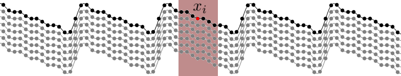
Figure 2: Surface true sources (black), and shifted true sources (gray). Matching the color code in Figure 1, the sources giving rise to “local” interactions for the given target point $x_{i}$ are contained in the region shaded in pink. The accelerated algorithm in Section 5.5 below produces $\tilde{D}_{\mathrm{reg}}^{\Delta x}(x_{i})$ (equation (48)) by subtraction of incorrect local contributions in an FFT-based “all-to-all” operator, followed by addition of the correct local contributions.

In order to accelerate the evaluation of the operator $\tilde{D}_{\mathrm{reg}}^{\Delta x}$, at first we disregard the shifted true sources (gray points in Figure 2) and we restrict attention to the surface true-sources (black dots) that are contained within a given cell $c^{q}$. In preparation for FFT acceleration we seek to represent the field generated by the latter sources in two different ways. As indicated in what follows, the equivalent sources are to be located in “Horizontal” and “Vertical” sets $\Lambda_{q}^{H}$ and $\Lambda_{q}^{V}$ of equispaced discretization points,

$$\Lambda_{q}^{\lambda}=\{\mathbf{y}_{s}^{\lambda,q}:s=1,\dots,n_{\mathrm{eq}}\}\qquad(\lambda=H,V),$$ (56)

contained on (slight extensions of) the horizontal and vertical sides of $c^{q}$, respectively; see Figure 3. (In the examples considered in this chapter each one of the extended sets $\Lambda_{q}^{H}$ and $\Lambda_{q}^{V}$ contain approximately 20% more equivalent-source points than are contained on each pair of parallel sides of the squares $c^{q}$ themselves. Such extensions provide slight accuracy enhancements as discussed in [7].) The resulting equivalent-source approximation, which is described in detail in Section 5.2, is valid and highly accurate outside the square domain $\mathcal{S}_{q}$ of side $3L$ and concentric with $c^{q}$:

$$\mathcal{S}_{q}=\bigcup_{-1\leq m,n\leq 1}\Big{(}c^{q}+(n,m)L\Big{)}.$$ (57)

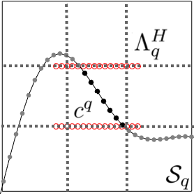
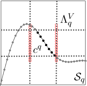
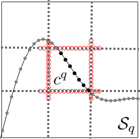
Figure 3: “Free-Space” Equivalent source geometry. The true sources within $c^{q}$ (resp. outside $c^{q}$) are displayed as solid black (resp. gray) circles. The left, center and right images depict in red unfilled circles the horizontal set $\Lambda_{q}^{H}$, the vertical set $\Lambda_{q}^{V}$, and the union $\Lambda_{q}^{H}\cup\Lambda_{q}^{V}$, respectively.

Importantly, for each $\lambda$ (either $\lambda=H$ or $\lambda=V$) the union of $\Lambda^{\lambda}_{q}$ for all $q$ (equation (78) below) is a Cartesian grid, and thus facilitates evaluation of certain necessary discrete convolutions by means of FFTs, as desired.

The proposed acceleration procedure is described below, starting with the computation of the equivalent-source densities (Section 5.2) and following with the incorporation of shifted equivalent sources and consideration of an associated validity criterion (Section 5.3). This validity criterion induces a decomposition of the operator $\tilde{D}_{\mathrm{reg}}^{\Delta x}$ into two terms (Section 5.4), each one of can be produced via certain FFT-based convolutions (Section 5.5). A reconstruction of needed surface fields is then produced (Section 5.6), and, finally, the overall fast high-order solver for equation (26) is presented (Section 5.7). For convenience, shifted and unshifted “punctured Green functions” $\Phi_{j}:\mathbb{R}^{2}\times\mathbb{R}^{2}\to\mathbb{C}$ and $\Phi:\mathbb{R}^{2}\times\mathbb{R}^{2}\to\mathbb{C}$ are used in what follows which, in terms of the two-dimensional observation and integration variables $\mathbf{x}=(x_{1},x_{2})\in\mathbb{R}^{2}$ and $\mathbf{y}=(y_{1},y_{2})\in\mathbb{R}^{2}$, are given by

$$\Phi_{j}(\mathbf{x},\mathbf{y})=\left\{\begin{array}[]{cc}G_{j}(x_{1}-y_{1},x_{2}-y_{2})&\mbox{ for }\mathbf{x}\neq\mathbf{y}\\ 0&\mbox{ for }\mathbf{x}=\mathbf{y}\end{array}\right.\quad\mbox{and}\quad\Phi=\Phi_{0}.$$ (58)

5.2 Equivalent-source representation I: surface true sources

As indicated above, this section provides an equivalent-source representation of the contributions to the quantity $\tilde{D}_{\mathrm{reg}}^{\Delta x}[\mu_{1},\dots,\mu_{N}](x_{i})$ in (48) that arise from surface true sources only (the solid black points in Figure 2). To do this we define

$$\psi^{q}(\mathbf{x})=\sum_{(x_{\ell},f(x_{\ell}))\,\in\,c^{q}}\left(\mu_{\ell}\;\frac{\partial}{\partial n_{y}}\Phi(\mathbf{x},\mathbf{y})\big{|}_{\mathbf{y}=(x_{\ell},f(x_{\ell}))}\right)(\Delta s)_{\ell},$$ (59)

which denotes the field generated by all of the surface true-sources located within the cell $c^{q}$. In the equivalent-source approach, the function $\psi^{q}$ is evaluated, with prescribed accuracy, by a fast procedure based on use of certain “horizontal” and “vertical” representations, which are valid, within the given accuracy tolerance, for values of $\mathbf{x}$ outside $\mathcal{S}_{q}$. Each of those representations is given by a sum of monopole and dipole equivalent-sources supported on the corresponding equispaced mesh $\Lambda_{q}^{\lambda}$ (56) ($\lambda=H$ or $\lambda=V$).

To obtain the desired representation a least-squares problem is solved for each cell $c^{q}$ (cf. [7]). In detail, for $\lambda=H$ and $\lambda=V$ and for each $q$, an approximate representation of the form

$$\psi^{q}(\mathbf{x})\approx\varphi^{q,\lambda}(\mathbf{x}),\quad\mbox{where}\quad\varphi^{q,\lambda}(\mathbf{x})=\sum_{s=1}^{n_{eq}}\left(\Phi(\mathbf{x},\mathbf{y}_{s}^{q,\lambda})\xi_{s}^{q,\lambda}+\frac{\partial}{\partial\nu(y)}\Phi(\mathbf{x},\mathbf{y}_{s}^{q,\lambda})\zeta_{s}^{q,\lambda}\right)$$ (60)

is sought, where $\xi_{s}^{q,\lambda}$ and $\zeta_{s}^{q,\lambda}$ are complex numbers (the “equivalent-source densities”), and where $\nu(y)$ denotes the normal to $\Lambda_{q}^{\lambda}$. The densities $\xi_{s}^{q,\lambda}$ and $\zeta_{s}^{q,\lambda}$ are obtained as the QR-based solutions [17] of the oversampled least-squares problem

$$\min_{(\xi_{s}^{q,\lambda},\zeta_{s}^{q,\lambda})}\sum_{t=1}^{n_{\mathrm{coll}}}\left|\psi^{q}(\mathbf{x}^{q}_{t})-\sum_{s=1}^{n_{eq}}\left(\Phi(\mathbf{x}^{q}_{t},\mathbf{y}_{s}^{q,\lambda})\xi_{s}^{q,\lambda}+\frac{\partial}{\partial n_{y}}\Phi(\mathbf{x}^{q}_{t},\mathbf{y}_{s}^{q,\lambda})\zeta_{s}^{q,\lambda}\right)\right|^{2},$$ (61)

where $\{\mathbf{x}_{t}^{q}\}_{t=1,\dots,n_{\mathrm{coll}}}$ is a sufficiently fine discretization of $\partial\mathcal{S}^{q}$, which in general may be selected arbitrarily, but which we generally take to equal the union of equispaced discretizations of the sides of $\partial\mathcal{S}^{q}$ (as displayed in Figure 4). Under these conditions, the equivalent source representation $\varphi^{q,\lambda}$ matches the field values $\psi^{q}(\mathbf{x})$ for $\mathbf{x}$ on the boundary of $\mathcal{S}^{q}$ within the prescribed tolerance. Since $\varphi^{q,\lambda}$ and $\psi^{q}(\mathbf{x})$ are both solutions of the Helmholtz equation with wavenumber $\mathrm{k}$ outside $\mathcal{S}^{q}$, it follows that $\varphi^{q,\lambda}$ agrees closely with $\psi^{q}(\mathbf{x})$ through the exterior of $\mathcal{S}^{q}$ as well [7]. The equivalent-source approximation and its accuracy outside of $\mathcal{S}_{q}$ is demonstrated in Figure 4 for the case $\lambda=H$ (“horizontal” representation).

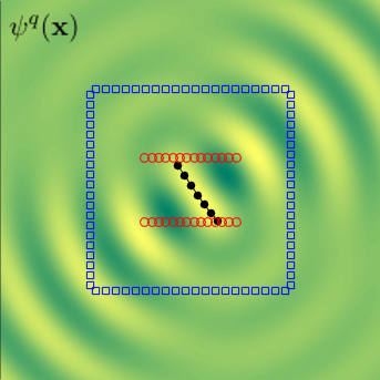
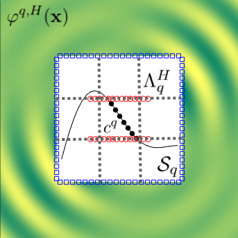
Figure 4: Left: Field $\psi^{q}(\mathbf{x})$ generated by the surface true sources (solid black circles), evaluated throughout space. Center: Approximate field $\varphi^{q,H}(\mathbf{x})$ generated by the equivalent sources (unfilled red circles), evaluated outside $\mathcal{S}^{q}$. Right: approximation error $|\psi^{q}(\mathbf{x})-\varphi^{q,H}(\mathbf{x})|$ outside $\mathcal{S}^{q}$ (in $\log_{10}$ scale). Collocation points $\mathbf{x}_{t}\in\partial\mathcal{S}^{q}$ are displayed as blue squares. According to the right image, the error for this test case ($\mathrm{k}=10$, $L=0.3$, $n_{\mathrm{eq}}=10$, $n_{\mathrm{coll}}=80$) is smaller than $10^{-12}$ everywhere in the validity region $\left\{x\in\mathbb{R}^{2}:x\not\in\mathcal{S}^{q}\right\}$..

Remark 10.

It is easy to see that the equivalent source densities $(\xi_{s}^{q,\lambda},\zeta_{s}^{q,\lambda})$ are $\alpha$-quasi periodic quantities, in the sense that given two cells, $c^{q}$ and $c^{q^{\prime}}$, where $c^{q^{\prime}}$ is displaced from $c^{q}$, in the horizontal direction, by an integer multiple $pd$ of the period $d$, we have $(\xi_{s}^{\lambda,q^{\prime}},\zeta_{s}^{\lambda,q^{\prime}})=e^{\mathrm{i}\alpha pd}(\xi_{s}^{\lambda,q},\zeta_{s}^{\lambda,q})$. To check this note that, since the corresponding density $\mu_{\ell}$ is itself $\alpha$-quasi periodic (equation (36)), in view of (59) it follows that so is the quantity $\psi^{q}(\mathbf{x}^{r}_{t})$ in (61). In particular, we have $\psi^{q^{\prime}}(\mathbf{x}^{q^{\prime}}_{t})=e^{\mathrm{i}\alpha pd}\psi^{q}(\mathbf{x}^{q}_{t})$. Since, additionally, $\Phi(\mathbf{x}^{q^{\prime}}_{t},\mathbf{y}_{s}^{\lambda,q^{\prime}})=\Phi(\mathbf{x}^{q}_{t},\mathbf{y}_{s}^{\lambda,q})$, we conclude that the least square problems (61) for $q$ and $q^{\prime}$ are equivalent, and the desired $\alpha$-quasiperiodicity of $(\xi_{s}^{q,\lambda},\zeta_{s}^{q,\lambda})$ follows.

5.3 Equivalent-source representation II: shifted true sources

In order to incorporate shifted true sources within the equivalent source representation we define the quantity

$$\psi_{j}^{q}(\mathbf{x})=\sum_{(x_{\ell},f(x_{\ell}))\,\in\,c^{q}}\left(\mu_{\ell}\;\frac{\partial}{\partial n_{y}}\Phi_{j}(\mathbf{x},\mathbf{y})\big{|}_{\mathbf{y}=(x_{\ell},f(x_{\ell}))}\right)(\Delta s)_{\ell}$$ (62)

which, in view of in view of (58), contains some of the contributions on the right hand side of (48). (With reference to (24), note that a term in the sum (62) coincides with a corresponding term in (48) if and only if $1-S_{\gamma,a}^{f}(x_{i},x_{\ell})=1$. For $\mathbf{y}=(x_{\ell},f(x_{\ell}))\in c^{q}$, the latter relation certainly holds provided $\mathbf{x}=(x_{i},f(x_{i}))$ is sufficiently far from $c^{q}$. But there are other pairs $(\mathbf{x,y})$ for which this this relation holds; see Section 5.4 below for details.)

In view of (11), the field $\psi_{j}^{q}$ in (62) includes contributions from all surface sources contained within the cell $c^{q}$ (solid black dots in Figure 5), as well as all of the shifted true sources that lie below them (which are displayed as gray dots in Figure 5). Importantly, as illustrated in Figure 5, these shifted sources may or may not lie within $c^{q}$.

In order to obtain an equivalent-source approximation of the shifted-true-source quantity $\psi_{j}^{q}$ in (62) which is analogous to the approximation (60) for the surface true sources, we consider the easily-checked relation

$$\psi_{j}^{q}(\mathbf{x})=\sum_{m=0}^{j}(-1)^{m}C_{m}^{j}\psi^{q}(\mathbf{x}-m\bar{h}),$$ (63)

where $\bar{h}=(0,h)$, and we use the approximation $\psi^{q}(\mathbf{x}-m\bar{h})\approx\varphi^{q,\lambda}(\mathbf{x}-m\bar{h})$ which follows by employing (60) at the point $\mathbf{x}-m\bar{h}$, for each $m$. Since, in view of the relation $\Phi(\mathbf{x}+\mathbf{z},\mathbf{y})=\Phi(\mathbf{x},\mathbf{y}-\mathbf{z})$, we have

$$\varphi^{q,\lambda}(\mathbf{x}-m\bar{h})=\sum_{s=1}^{n_{eq}}\left(\Phi(\mathbf{x},\mathbf{y}_{s}^{q,\lambda}+m\bar{h})\xi_{s}^{q,\lambda}+\frac{\partial}{\partial\nu(y)}\Phi(\mathbf{x},\mathbf{y}_{s}^{q,\lambda}+m\bar{h})\zeta_{s}^{q,\lambda}\right),$$ (64)

summing (64) over $m$ yields the desired approximation:

$$\psi_{j}^{q}(\mathbf{x})\approx\varphi_{j}^{q,\lambda}(\mathbf{x}),\quad\mbox{where}\quad\varphi_{j}^{q,\lambda}(\mathbf{x})=\sum_{s=1}^{n_{eq}}\left(\Phi_{j}(\mathbf{x},\mathbf{y}_{s}^{q,\lambda})\xi_{s}^{q,\lambda}+\frac{\partial}{\partial\nu(y)}\Phi_{j}(\mathbf{x},\mathbf{y}_{s}^{q,\lambda})\zeta_{s}^{q,\lambda}\right).$$ (65)

The shifted-equivalent-source approximation (65) is a central element of the proposed acceleration approach. Noting that, for each $m$, the approximation (64) is valid for points $\mathbf{x}$ outside a translated domain $\mathcal{S}^{q}-m\bar{h}$, it follows that, calling

$$\widehat{\mathcal{S}}_{j}^{q}=\bigcup_{m=0}^{j}\left(\mathcal{S}^{q}-m\bar{h}\right),$$ (66)

the overall approximation (65) is valid for all $\mathbf{x}\not\in\widehat{\mathcal{S}}_{j}^{r}$. Thus, letting

$$\mathcal{S}_{j}^{q}=\bigcup_{\{r\,:\,c^{r}\cap\widehat{\mathcal{S}}_{j}^{q}\neq\emptyset\}}c^{r},$$ (67)

(which equals the smallest union of cells $c^{r}$ that contains $\widehat{\mathcal{S}}_{j}^{q}$), it follows, in particular, that (65) is a valid approximation for all $\mathbf{x}\not\in\mathcal{S}_{j}^{q}$.

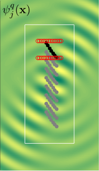
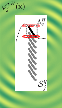
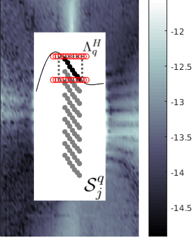
Figure 5: Left: Field $\psi_{j}^{q}(\mathbf{x})$ generated by the combination of the true sources (solid black circles) and their shifted copies (solid gray circles). Center: Approximate field $\varphi_{j}^{q,H}(\mathbf{x})$ generated by shifted equivalent sources (unfilled red circles). Right: approximation error $|\psi_{j}^{q}(\mathbf{x})-\varphi_{j}^{q,H}(\mathbf{x})|$ outside $\mathcal{S}_{j}^{q}$ (in $\log_{10}$ scale). According to the right image, the error for this test case ($\mathrm{k}=10$, $L=0.3$, $n_{\mathrm{eq}}=10$, $n_{\mathrm{coll}}=80$) is smaller than $10^{-12}$ everywhere in the validity region $\left\{x\in\mathbb{R}^{2}:x\not\in\mathcal{S}_{j}^{q}\right\}$.

5.4 Decomposition of $\tilde{D}_{\mathrm{reg}}^{\Delta x}$ in “intersecting” and “non-intersecting” contributions

This section introduces a decomposition of the operator $\tilde{D}_{\mathrm{reg}}^{\Delta x}$ as a sum of two terms. With reference to Remark 8, and denoting by $\overline{A}$ the closure of a set $A$ (the union of the set and its boundary), we define the first term as

$$\psi_{j}^{ni,q}:\overline{c^{q}}\to\mathbb{C},\qquad\psi^{ni,q}_{j}(\mathbf{x})=\sum_{\{r\in\mathbb{Z}\,:\,c^{q}\cap\mathcal{S}_{j}^{r}=\emptyset\}}\psi^{r}_{j}(\mathbf{x}),\qquad(\mathbf{x}\in\overline{c^{q}}).$$ (68)

Clearly, for $\mathbf{x}\in\overline{c^{q}}$, the quantity $\psi_{j}^{ni,q}(\mathbf{x})$ contains the “non-intersecting” contributions—that is, contributions arising from sources contained in cells $c^{r}\subset\Omega_{\infty}$, $-\infty\leq r\leq\infty$ (cf. equation (55)), such that $\mathcal{S}_{j}^{r}$ does not intersect $c^{q}$, and for which therefore, according to Section 5.3, the approximation (65) is valid. Since the operator $\tilde{D}_{\mathrm{reg}}^{\Delta x}$ acts on spaces of functions defined on $\Gamma$, in what follows we will often evaluate $\psi_{j}^{ni,q}$ at points $\mathbf{x}\in\overline{c^{q}}$ of the form $\mathbf{x}=(x_{i},f(x_{i}))\in\overline{c^{q}}$. For $\mathbf{x}=(x_{i},f(x_{i}))\in\overline{c^{q}}$, then, the second term equals, naturally,

$$\psi^{\textit{int},q}_{j}\Big{(}x_{i},f(x_{i})\Big{)}=\tilde{D}_{\mathrm{reg}}^{\Delta x}[\mu_{1},\dots,\mu_{N}](x_{i})-\psi^{ni,q}_{j}\Big{(}x_{i},f(x_{i})\Big{)},\qquad(x_{i},f(x_{i}))\in c^{q}.$$ (69)

In view of definitions (62) and (68), the field $\psi_{j}^{ni,q}(\mathbf{x})$ can alternatively by expressed in the form

$$\psi_{j}^{ni,q}(\mathbf{x})=\sum_{\{\ell\in\mathbb{Z}\,:\,(x_{\ell},f(x_{\ell}))\,\in\,c^{r}\,\footnotesize{\mbox{with}}\;c^{q}\cap\mathcal{S}_{j}^{r}=\emptyset\}}\left(\mu_{\ell}\;\frac{\partial}{\partial n_{y}}\Phi_{j}(\mathbf{x},\mathbf{y})\big{|}_{\mathbf{y}=(x_{\ell},f(x_{\ell}))}\right)(\Delta s)_{\ell}.$$ (70)

Note that all non-intersecting contributions to a point $\mathbf{x}=(x_{i},f(x_{i}))\in c^{q}$ arise from integration points $(x_{\ell},f(x_{\ell}))$ that are at a distance larger than the side $L$ of $c^{q}$. Thus, in view of Remark 9 ($a<L$), we have $S_{\gamma,a}^{f}(x_{i},x_{\ell})=0$ for all non-intersecting contributions. In view of (48) and (70), then, we obtain

$$\psi^{\textit{int},q}_{j}\Big{(}x_{i},f(x_{i})\Big{)}=\sum_{\{\ell\in\mathbb{Z}\,:\,(x_{\ell},f(x_{\ell}))\,\in\,c^{r}\,\small{\mbox{with}}\;c^{q}\cap\mathcal{S}_{j}^{r}\neq\emptyset\}}\mu_{\ell}(1-S_{\gamma,a}^{f}(x_{i},x_{\ell}))\partial_{\nu^{\prime}}G_{j}(x_{i},x_{\ell})(\Delta s)_{\ell}.$$ (71)

The following two sections (5.5 and 5.6) present an efficient evaluation strategy for the quantities $\psi^{ni,q}_{j}(\mathbf{x})$ over $\Gamma\cap c^{q}$, for $q=1,\dots,n_{\mathrm{cell}}$. This strategy relies on use of the approximation

$$\psi^{ni,q}_{j}(\mathbf{x})\approx\varphi^{ni,q,\lambda}_{j}(\mathbf{x});\qquad\varphi^{ni,q,\lambda}_{j}(\mathbf{x})=\sum_{\{r\in\mathbb{Z}\,:\,c^{q}\cap\mathcal{S}_{j}^{r}=\emptyset\}}\;\sum_{s=1}^{n_{\mathrm{eq}}}\left(\Phi_{j}(\mathbf{x},\mathbf{y}_{s}^{r,\lambda})\xi_{s}^{r,\lambda}+\frac{\partial}{\partial n_{y}}\Phi_{j}(\mathbf{x},\mathbf{y}_{s}^{r,\lambda})\zeta_{s}^{r,\lambda}\right),$$ (72)

(for $\mathbf{x}\in c^{q}$) which can be obtained by substituting equation (65) into (68). As shown in Section 5.5, the quantities $\varphi^{ni,q,\lambda}_{j}(\mathbf{x})$ in (72) ($q=1,\dots,n_{\mathrm{cell}}$) are related to a single discrete Cartesian convolution that can be evaluated rapidly by means of the FFT algorithm. Once $\psi^{ni,q}(\mathbf{x})$ has been evaluated (by means of $\varphi^{ni,q,\lambda}_{j}$), the remaining “local” contributions $\psi^{\textit{int},q}_{j}$ to $\tilde{D}_{\mathrm{reg}}^{\Delta x}$ can be incorporated using (71) at a small computational cost. The overall fast high-order numerical algorithm for evaluation of the operator on the left-hand side of equation (26) (which also incorporates the implementations of the operators $\tilde{D}^{\Delta x}_{\mathrm{sing}}$ and $D_{M}^{\Delta x}$ presented in Section 4.3) together with the associated fast iterative solver, are then summarized in Section 5.7.

5.5 Approximation of $\psi^{ni,q}_{j}$ via global and local convolutions at FFT speeds

In order to accelerate the evaluation of $\psi^{ni,q}_{j}$ by means of the FFT algorithm we introduce the quantity

$$\varphi^{\textit{all},\lambda}_{j}(\mathbf{x})=\sum_{r\in\mathbb{Z}}\sum_{s=1}^{n_{\mathrm{eq}}}\left(\Phi_{j}(\mathbf{x},\mathbf{y}_{s}^{r,\lambda})\xi_{s}^{r,\lambda}+\frac{\partial}{\partial n_{y}}\Phi_{j}(\mathbf{x},\mathbf{y}_{s}^{r,\lambda})\zeta_{s}^{r,\lambda}\right)$$ (73)

which incorporates the non-intersecting terms already included in (72) as well as undesired “intersecting” (local) terms. For each $q$, the sum of all undesired intersecting terms for the domain $\overline{c^{q}}$ is a function $\varphi^{\textit{int},q,\lambda}_{j}:\overline{c^{q}}\to\mathbb{C}$ given by

$$\varphi^{\textit{int},q,\lambda}_{j}(\mathbf{x})=\sum_{\begin{subarray}{c}r\in\mathcal{L}(q)\\ 1\leq s\leq n_{\mathrm{eq}}\end{subarray}}\left(\Phi_{j}(\mathbf{x},\mathbf{y}_{s}^{r,\lambda})\xi_{s}^{r,\lambda}+\frac{\partial}{\partial n_{y}}\Phi_{j}(\mathbf{x},\mathbf{y}_{s}^{r,\lambda})\zeta_{s}^{r,\lambda}\right),\quad\mbox{where}\;\mathcal{L}(q)=\{r\in\mathbb{Z}:c^{q}\subset\mathcal{S}_{j}^{r}\}.$$ (74)

Since, by construction, $c^{q}\cap\mathcal{S}^{r}_{j}\neq\emptyset$ if and only if $c^{q}\subset\mathcal{S}^{r}_{j}$, in view of (72) we clearly have

$$\varphi^{ni,q,\lambda}_{j}=\varphi^{\textit{all},\lambda}_{j}-\varphi^{\textit{int},q,\lambda}_{j}.$$ (75)

This relation reduces the evaluation of $\varphi^{ni,q,\lambda}_{j}$ to evaluation of the $q$-independent quantity (73) and the $q$-dependent quantity (74).

The expression (73) for $\varphi^{\textit{all},\lambda}_{j}$ requires the evaluation of an infinite sum. Exploiting the fact that, as indicated in Remark 10, the equivalent sources $(\xi_{s}^{r,\lambda},\zeta_{s}^{r,\lambda})$ are $\alpha$-quasi-periodic quantities, a more convenient expression can be obtained. Indeed, defining

$$\widetilde{\Phi}_{j}^{\textit{qper}}:\mathbb{R}^{2}\times\mathbb{R}^{2}\to\mathbb{C},\qquad\widetilde{\Phi}_{j}^{\textit{qper}}(\mathbf{x},\mathbf{y})=\left\{\begin{array}[]{cc}\tilde{G}_{j}^{\textit{qper}}(x_{1}-y_{1},x_{2}-y_{2})&\mbox{ for }\mathbf{x}\neq\mathbf{y}\\ 0&\mbox{ for }\mathbf{x}=\mathbf{y}\end{array}\right.$$ (76)

in terms of the variables $\mathbf{x}=(x_{1},x_{2})\in\mathbb{R}^{2}$ and $\mathbf{y}=(y_{1},y_{2})\in\mathbb{R}^{2}$, we can express $\varphi^{\textit{all},\lambda}_{j}$ as the sum

$$\varphi^{\textit{all},\lambda}_{j}(\mathbf{x})=\sum_{r=1}^{n_{\mathrm{cell}}}\sum_{s=1}^{n_{\mathrm{eq}}}\left(\widetilde{\Phi}_{j}^{\textit{qper}}(\mathbf{x},\mathbf{y}_{s}^{r,\lambda})\xi_{s}^{r,\lambda}+\frac{\partial}{\partial n_{y}}\widetilde{\Phi}_{j}^{\textit{qper}}(\mathbf{x},\mathbf{y}_{s}^{r,\lambda})\zeta_{s}^{r,\lambda}\right)$$ (77)

of finitely many terms, each one of which contains $\widetilde{\Phi}_{j}^{\textit{qper}}$.

In order to evaluate the quantities $\varphi^{\textit{all},\lambda}_{j}$ and $\varphi^{\textit{int},q,\lambda}_{j}$ by means of the FFT algorithm we use the equivalent-source meshes $\Lambda_{q}^{\lambda}$ introduced in Section 5.1 (and depicted in Figure 3) and we define, for $\lambda=H,V$, the “global” and “local” Cartesian grids

$$\Pi_{\lambda}^{\textit{per}}=\bigcup_{\{r\in\mathbb{Z}\;:\;c^{r}\subseteq\Omega_{per}\}}\Lambda^{\lambda}_{r}\qquad\mbox{and}\qquad\Pi_{\lambda}^{q}=\bigcup_{\{r\in\mathbb{Z}\;:\;c^{q}\subset\mathcal{S}_{j}^{r}\}}\Lambda^{\lambda}_{r}.$$ (78)

The following two sections describe algorithms which rapidly evaluate these quantities by means of FFTs. The evaluation of $\psi^{ni,q}_{j}$ (which is the main goal of Section 5.5) then follows directly, as indicated in Section 5.5.3.

5.5.1 Evaluation of $\varphi^{\textit{all},\lambda}_{j}$ in $\Pi_{\lambda}$ via a global convolution

In order to express $\varphi^{\textit{all},\lambda}_{j}$ as a convolution, for $\mathbf{y^{\prime}}\in\Pi_{\lambda}^{\textit{per}}$ and $\lambda=H,V$ we define the sums

$$\xi^{\textit{all},\lambda}(\mathbf{y^{\prime}})=\sum_{\begin{subarray}{c}1\leq r\leq n_{\mathrm{cell}}\\ 1\leq s\leq n_{\mathrm{eq}}\\ \mathbf{y}_{s}^{r,\lambda}=\mathbf{y^{\prime}}\end{subarray}}\xi_{s}^{r,\lambda}\qquad\mbox{ and }\qquad\zeta^{\textit{all},\lambda}(\mathbf{y^{\prime}})=\sum_{\begin{subarray}{c}1\leq r\leq n_{\mathrm{cell}}\\ 1\leq s\leq n_{\mathrm{eq}}\\ \mathbf{y}_{s}^{r,\lambda}=\mathbf{y^{\prime}}\end{subarray}}\zeta_{s}^{r,\lambda}$$ (79)

of equivalent source densities $\xi_{s}^{r,\lambda}$ and $\zeta_{s}^{r,\lambda}$, respectively ($1\leq r\leq n_{\mathrm{cell}}$), that are supported at a given point $\mathbf{y^{\prime}}\in\Pi_{\lambda}^{\textit{per}}$. We note that two and even four contributions may arise at a point $\mathbf{y^{\prime}}\in\Pi_{\lambda}^{\textit{per}}$—as $\mathbf{y^{\prime}}$ may lie on a common side of two neighboring cells, and, in some cases, on the intersection of four different sets $\Lambda_{q}^{\lambda}$—on account of overlap of the extended regions described in Section 5.1 and depicted in Figure 3.

Replacing (79) in (77), we arrive at the discrete-convolution expression

$$\varphi^{\textit{all},\lambda}_{j}(\mathbf{x})=\sum_{\mathbf{y^{\prime}}\,\in\Pi_{\lambda}^{\textit{per}}}\left(\widetilde{\Phi}_{j}^{\textit{qper}}(\mathbf{x},\mathbf{y^{\prime}})\xi^{\textit{all},\lambda}(\mathbf{y^{\prime}})+\frac{\partial}{\partial n_{y}}\widetilde{\Phi}_{j}^{\textit{qper}}(\mathbf{x},\mathbf{y^{\prime}})\zeta^{\textit{all},\lambda}(\mathbf{y^{\prime}})\right),\quad\mathbf{x}\in\Pi_{\lambda}^{\textit{per}},$$ (80)

for the quantity $\varphi^{\textit{all},\lambda}_{j}$ on the mesh $\Pi_{\lambda}^{\textit{per}}$. The evaluation of this convolution can be performed by a standard FFT-based procedure in $O(M\log M)$ operations, where $M=O(n_{\mathrm{cell}}n_{eq})$ denotes the number of elements in $\Pi_{\lambda}^{\textit{per}}$. Note that, per equation (76), this global FFT algorithm requires the values of the quasi-periodic Green function $\tilde{G}^{\textit{qper}}_{j}(X,Y)$ (see also Remark 11 below) at points $(X,Y)$ in the “evaluation grid” $\widehat{\Pi}_{\lambda}^{\textit{per}}=\{\mathbf{x}-\mathbf{y}:\mathbf{x},\mathbf{y}\in\Pi_{\lambda}^{\textit{per}}\}$. In fact, this is the only point in the accelerated algorithm that requires use of the quasi-periodic Green function.

Remark 11.

An efficient strategy for the evaluation of $\tilde{G}^{\textit{qper}}_{j}(X,Y)$ at a given point was presented in Section 3.2, which makes use of both spectral and spatial representations of this function. Additional performance gains are obtained in the present context by exploiting certain symmetries in the evaluation grid $\widehat{\Pi}_{\lambda}^{\textit{per}}$. The identity $\tilde{G}^{\textit{qper}}_{j}(X+d,Y)=e^{i\alpha d}\tilde{G}^{\textit{qper}}_{j}(X,Y)$ is used to restrict the evaluation of the function $\tilde{G}^{\textit{qper}}_{j}(X,Y)$ at, say, only positive values of $X$; for the $j=0$ case, the identity $\tilde{G}^{\textit{qper}}_{0}(X,Y)=\tilde{G}^{\textit{qper}}_{0}(X,-Y)$ is similarly used to restrict evaluation of $\tilde{G}^{\textit{qper}}_{0}(X,Y)$ to positive values of $Y$. Further, since the spectral series (17) is a sum of exponentials which can expressed as products of exponentials that depend on $X$ and $Y$ separately, the spectral series can be evaluated efficiently by utilizing precomputed values of the required single-variable exponentials—with limited computing and storage cost. For an efficient implementation of the spatial series, finally, asymptotic expansions of the Hankel functions as proposed in [4] are also used. The overall strategy produces the required values of $\tilde{G}^{\textit{qper}}_{j}$ over the necessary evaluation grid $\widehat{\Pi}_{\lambda}^{\textit{per}}$ in a highly efficient manner.

5.5.2 Evaluation of $\varphi^{\textit{int},q,\lambda}_{j}$ in $\Pi_{\lambda}^{q}$ via a local convolution

In order to express $\varphi^{\textit{int},q,\lambda}_{j}$ (equation (74)) as a convolution, for $\mathbf{y^{\prime}}\in\Pi_{\lambda}^{q}$, we define the sums

$$\xi^{q,\lambda}(\mathbf{y^{\prime}})=\sum_{\begin{subarray}{c}r\in\mathcal{L}(q)\\ 1\leq s\leq n_{\mathrm{eq}}\\ \mathbf{y}_{s}^{r,\lambda}=\,\mathbf{y^{\prime}}\end{subarray}}\xi_{s}^{r,\lambda}\qquad\mbox{ and }\qquad\zeta^{q,\lambda}(\mathbf{y^{\prime}})=\sum_{\begin{subarray}{c}r\in\mathcal{L}(q)\\ 1\leq s\leq n_{\mathrm{eq}}\\ \mathbf{y}_{s}^{r,\lambda}=\,\mathbf{y^{\prime}}\end{subarray}}\zeta_{s}^{r,\lambda}$$ (81)

of equivalent source densities $\xi_{s}^{r,\lambda}$ and $\zeta_{s}^{r,\lambda}$, respectively, that are supported at the point $\mathbf{y^{\prime}}\in\Pi_{\lambda}^{q}$, where $r$ lies in the local set of indexes $\mathcal{L}(q)$ defined in (74). Note that, the set $\mathcal{L}(q)$ contains integers $r$ that may lie outside the range $1\leq r\leq n_{\mathrm{cell}}$. In such cases, in order to avoid use of equivalent source densities that lie outside the reference periodicity domain $\Omega^{\textit{per}}$, the $\alpha$-quasiperiodicity of $\xi_{s}^{r,\lambda}$ and $\zeta_{s}^{r,\lambda}$ (Remark 10) is utilized to re-express the sums in (81) in terms of equivalent sources $\xi_{s}^{r,\lambda}$ and $\zeta_{s}^{r,\lambda}$ for which $1\leq r\leq n_{\mathrm{cell}}$. Additionally note that, as in Section 5.5.1, two and even four contributions may arise in the sums (81) for a given point $\mathbf{y^{\prime}}\in\Pi_{\lambda}^{q}$.

Replacing (81) in (74) yields the discrete-convolution expression

$$\varphi^{\textit{int},q,\lambda}_{j}(\mathbf{x})=\sum_{\mathbf{y^{\prime}}\,\in\Pi_{\lambda}^{q}}\left(\Phi_{j}(\mathbf{x},\mathbf{y^{\prime}})\xi^{q,\lambda}(\mathbf{y^{\prime}})+\frac{\partial}{\partial n_{y}}\Phi_{j}(\mathbf{x},\mathbf{y^{\prime}})\zeta^{q,\lambda}(\mathbf{y^{\prime}})\right),\quad\mathbf{x}\in\Pi_{\lambda}^{q},$$ (82)

which can be evaluated for all $\mathbf{x}\in\Pi_{\lambda}^{q}$ by means of an FFT procedure, in $O(M_{q}\log M_{q})$ operations, where $M_{q}=O(n_{eq})$ denotes the number of elements in $\Pi^{q}_{\lambda}$. This time, the Green function $\Phi_{j}$ has to be evaluated on the “evaluation grid”

$$\widehat{\Pi}_{\lambda}^{q}=\{\mathbf{x}-\mathbf{y}:\mathbf{x},\mathbf{y}\in\Pi_{\lambda}^{q}\}.$$ (83)

Notice that the set $\widehat{\Pi}_{\lambda}^{q}$ is in fact independent of $q$.

5.5.3 Approximation of $\psi^{ni,q}_{j}$ on the boundary of $c^{q}$

Having obtained $\varphi^{\textit{int},q,\lambda}_{j}(\mathbf{x})$ and $\varphi^{\textit{all},\lambda}_{j}(\mathbf{x})$, the desired quantities $\varphi^{ni,q,\lambda}_{j}(\mathbf{x})$, for $\lambda=H,V$ follow from (75). For each $q$ ($1\leq q\leq n_{\mathrm{cell}}$) the resulting discrete values $\varphi^{ni,q,H}_{j}$ and $\varphi^{ni,q,V}_{j}$ are finally used to form the mesh functions

$$\varphi^{ni,q}_{j}:\overline{c^{q}}\cap(\Pi_{H}^{q}\cup\Pi_{V}^{q})\to\mathbb{C},\qquad\varphi^{ni,q}_{j}(\mathbf{x})=\varphi^{ni,q,\lambda}_{j}(\mathbf{x})\quad\mbox{ for }\quad\mathbf{x}\in\overline{c^{q}}\cap\Pi_{\lambda}^{q}\quad\mbox{and}\quad\lambda=H,V.$$ (84)

It is clear, by construction, that $\varphi^{ni,q}_{j}(\mathbf{x})$ is an approximation of $\psi^{ni,q}_{j}(\mathbf{x})$ for each element $\mathbf{x}$ in the discretization $\overline{c^{q}}\cap(\Pi_{H}^{q}\cup\Pi_{V}^{q})$ of the boundary of $c^{q}$. Using these approximate values, the next section presents a method for the high-order evaluation of $\psi^{ni,q}_{j}(\mathbf{x})$ at an arbitrary point within $c^{q}$, and thus, in particular, on the portion $\Gamma\cap c^{q}$ of the scattering surface $\Gamma$ contained within $c^{q}$.

5.6 Plane Wave representation of $\psi^{ni,q}_{j}$ within $c^{q}$

Since $\psi^{ni,q}_{j}(\mathbf{x})$ satisfies the Helmholtz equation within the cell $c^{q}$, and in view of Remark 7, this field can be obtained within that cell as the solution of the Dirichlet problem with values $\psi^{ni,q}_{j}(\mathbf{x})$ on the cell boundary. Using the approximate values $\varphi^{ni,q}_{j}$ of the field $\psi^{ni,q}_{j}(\mathbf{x})$ that are produced, on the discrete mesh $\overline{c^{q}}\cap(\Pi_{H}^{q}\cup\Pi_{V}^{q})$, by the fast algorithm described in Section 5.5, approximate values of the solution $\psi^{ni,q}_{j}(\mathbf{x})$ of this Dirichlet problem for $\mathbf{x}\in c^{q}$ are obtained [7] by means of a discrete plane wave expansion. Thus, using a number $n_{\mathrm{plw}}$ of plane waves, the proposed approximation for $\mathbf{x}\in c^{q}$ is thus given by the expression

$$\psi^{ni,q}_{j}(\mathbf{x})\approx\eta^{ni,q}_{j}(\mathbf{x})\quad\mbox{where}\quad\eta^{ni,q}_{j}(\mathbf{x})=\sum_{s=1}^{n_{\mathrm{plw}}}{w_{s}.e^{\mathrm{i}\mathrm{k}d_{s}\cdot\mathbf{x}}},\quad\mathbf{x}\in c^{q},$$ (85)

where the weights $w_{i}$ are obtained as the QR solution [17] of the least squares problem

$$\min_{\{w_{s}\}}\sum_{\mathbf{x}\in\overline{c^{q}}\cap(\Pi_{H}^{q}\cup\Pi_{V}^{q})}\left|\varphi^{ni,q}_{j}(\mathbf{x})-\sum_{s=1}^{n_{\mathrm{plw}}}{w_{s}.e^{\mathrm{i}\mathrm{k}d_{s}\cdot\mathbf{x}}}\right|^{2},\quad\mbox{where}\quad d_{s}=\left(\sin\left(\frac{2\pi s}{n_{\mathrm{plw}}}\right),\cos\left(\frac{2\pi s}{n_{\mathrm{plw}}}\right)\right).$$ (86)

This is the last necessary element in the proposed algorithm for fast approximate evaluation of the operator $\tilde{D}_{\mathrm{reg}}^{\Delta x}$. Using the various components introduced above in the present Section 5, Section 5.7 describes the overall proposed fast high-order solver.

5.7 Overall fast high-order solver for equation (26)

The overall solver described in what follows results as a modified version of the unaccelerated solver presented in Section 4.3: in the present accelerated solver the evaluation of the operator $\tilde{D}_{\mathrm{reg}}^{\Delta x}$ is carried out using the procedure described in Sections 5.1 through 5.6 instead of the straightforward $O(N^{2})$ approach used in Section 4.3. Algorithms 1 to 3 summarize the overall accelerated solution method.

Algorithm 1 Main program: solution of equation (53)

Run Initialization (Algorithm 2)

Run GMRES iterations, using the forward-map Algorithm 3, on the linear algebra problem (53)

Algorithm 2 Initialization

Obtain QR factors for (61) and (86) // Only once (they do not depend on $q$).

Evaluate $G_{j}^{\textit{qper}}$ on $\widehat{\Pi}_{\lambda}^{\textit{per}}$ // Remark 11.

Evaluate $G_{j}$ on $\widehat{\Pi}_{\lambda}^{q}$ // Only once ($\widehat{\Pi}_{\lambda}^{q}$ in (83) does not depend on $q$).

Precompute matrices for $\tilde{D}^{\Delta x}_{\mathrm{sing}}$ and $D^{\Delta x}_{M}$ // Equations (42) and (51).

Algorithm 3 Discrete forward map: $[\mu_{1},\dots,\mu_{n}]\to\left(\frac{1}{2}I+D^{\Delta x}\right)[\mu_{1},\dots,\mu_{n}]$

$\{(\xi_{s}^{q,\lambda},\zeta_{s}^{q,\lambda})\}\longleftarrow$ EqSources // Solve least squares problem (61).

$\{(\xi^{\textit{all},\lambda}_{\mathbf{y^{\prime}}},\zeta^{\textit{all},\lambda}_{\mathbf{y^{\prime}}})\}\longleftarrow$ GlobalEqSMerge // Combine equivalent sources (79).

$\{\varphi^{all,\lambda}_{j}\}\longleftarrow$ GlobalFFT // Evaluate (80) via FFT on the grid $\Pi_{\lambda}^{\textit{per}}$.

$\{(\xi^{q,\lambda}_{\mathbf{y^{\prime}}},\zeta^{q,\lambda}_{\mathbf{y^{\prime}}})\}\longleftarrow$ LocalEqSMerge // Combine equivalent sources (81).

$\{\varphi^{\textit{int},q,\lambda}_{j}\}\longleftarrow$ LocalFFT // Evaluate (82) via FFT on the grid $\Pi_{\lambda}^{q}$.

$\{\varphi^{ni,q,\lambda}_{j}\}\longleftarrow$ LocalSubtract // Subtract $\varphi^{\textit{int},q,\lambda}_{j}$ from $\varphi^{all,\lambda}_{j}$ (75).

$\{\varphi^{ni,q}_{j}\}\longleftarrow$ Combine-$\lambda$ // Combine $\varphi^{ni,q,H}_{j}$ and $\varphi^{ni,q,V}_{j}$ as in (84).

$\{w_{s}^{q}\}\longleftarrow$ PlaneWaveWeights // Solve least square problem (86).

$\psi^{ni,q}_{j}\dashleftarrow$ NonIntersecting // Use (85); $\mathbf{x}=(x_{i},f(x_{i}))\in c^{q}$.

$\psi^{\textit{int},q}_{j}\longleftarrow$ Intersecting // Use (71); $(x_{i},f(x_{i}))\in c^{q}$.

$\tilde{D}_{\mathrm{reg}}^{\Delta x}\dashleftarrow$ EvalRegular // Use (69), $\psi^{ni,q}_{j}(x_{i},f(x_{i}))$, $\psi^{\textit{int},q}_{j}(x_{i},f(x_{i}))$.

$\tilde{D}_{\mathrm{sing}}^{\Delta x}\longleftarrow$ EvalSingular // Use (42); $1\leq i\leq N$.

$D^{\Delta x}_{M}\longleftarrow$ EvalModes // Use (51); $1\leq i\leq N$.

$\left(\frac{1}{2}I+D^{\Delta x}\right)\longleftarrow$ AddOperators // Add $\frac{1}{2}I$, $\tilde{D}_{\mathrm{sing}}^{\Delta x}$, $\tilde{D}_{\mathrm{reg}}^{\Delta x}$ and $D^{\Delta x}_{M}$ (52)-(53).

Algorithm 3: Routines EqSource, GlobalFFT, etc. perform the tasks described in the corresponding comments on the right column, resulting on the values indicated by the left-pointing solid arrows. Dashed arrows indicate that an additional approximation is used in the assignment. Whenever the resulting values (on the left) depend on $q$ and/or $\lambda$, the operations are performed for $1\leq q\leq n_{\mathrm{cell}}$ and/or for $\lambda=H,V$, respectively.

The accuracy and efficiency of this algorithm is demonstrated in the following section.

Remark 12.

Once a solution $\mu$ of the integral equation (26) has been obtained, a single application of a slightly modified version of Algorithm 3 enables the evaluation of the scattered field $u^{scat}(\mathbf{x})$ in (23), and thus the total field $u(\mathbf{x})=u^{scat}(\mathbf{x})+u^{inc}(\mathbf{x})$, at all points $\mathbf{x}=(x,y)$ in a given two-dimensional domain—at a very moderate additional computational cost. In brief, the modified evaluation procedure only requires that equations (71) and (85), together with their dependencies, be implemented so as to produce the necessary scattered field $u^{scat}$ at all points where the fields are desired.

6 Numerical results

This section presents results of applications of the proposed algorithm to problems of scattering by perfectly conducting periodic rough surfaces, at both Wood and non-Wood configurations, with sinusoidal and composite rough surfaces (including randomly rough Gaussian surfaces), and through wide ranges of problem parameters—including grazing incidences and high period-to-wavelength and/or height-to-period ratios. The presentation is prefaced by a brief section concerning computational costs. For brevity, only results for the accelerated method are presented. In all cases these results compare favorably, in terms of computing times, accuracy and generality, with those provided by previous approaches. All computational results presented in this section were obtained from single-core runs on a 3.4GHz Intel i7-6700 processor with 4 Gb of memory.

6.1 Computing costs

The dependence of the computing cost of the algorithm on the size of the problem is subtle, as it includes costs components from various code elements (acceleration, integration, Green function evaluations, etc.), each one of which depends significantly on a variety of structural parameters—including the shift-parameter $h$, the various ratios $H/d$, $H/\lambda$, $d/\lambda$ involving the height $H$, the period $d$, and the wavelength $\lambda$, and the “roughness” of the surface, as quantified by the decay of the associated spectrum. Roughly speaking, however, the results in the present section suggest two important asymptotic regimes exist: (1) $d/\lambda$ grows as $H/\lambda$ is kept fixed; and, (2) Both $d/\lambda$ and $H/\lambda$ are allowed to grow simultaneously.

In case (1), which arises in the context of studies of scattering by randomly rough surfaces such as the Gaussian surfaces considered in Section 6.4, the cost of the algorithm grows at most linearly with the number of unknowns—regardless of the incidence angle, and including near grazing incidences. This favorable behavior stems from the decay experienced by the shifted Green function $G_{j}$ used in (14) as $d/\lambda$ grows while keeping a constant height $H/\lambda$ (cf. (13) and [4, Sec. 5.4]). As a result of this decay, the number $n_{\mathrm{per}}$ of terms necessary to obtain a prescribed error tolerance in the summation of (14) decreases as $d$ grows. In case (2), on the other hand, the computational cost is generally observed to range from $O(N)$ up to $O(N^{\frac{3}{2}})$, and it can even reach $O(N^{2})$ for extreme geometries.

The cost of the overall algorithm can be affected significantly by the value selected for the shift-parameter $h$ (or, rather, of the dimensionless parameter $h/\lambda$). On one hand, this parameter controls the rate of convergence of the spatial series for the shifted Green function: smaller values of $h/\lambda$ result in faster convergence of this series. On the other hand, however, use of very small values of $h/\lambda$ does give rise to certain ill-conditioning difficulties (which, for geometric reasons, become more and more pronounced as the grating-depths increase [4]). In particular, since, for a fixed $h/\lambda$ value, the distance between the scattering surface and the first shifted source decreases as the depth of the surface is increased, to avoid ill-conditioned-related accuracy losses it becomes necessary to use larger and larger values of $h/\lambda$ as the surface height grows. The selection of such larger $h/\lambda$ values, in turn, requires use of increasingly higher number of periods for the summation of the spatial periodic Green function to maintain accuracy. For the test cases considered in this paper, values of $h/\lambda$ in the range $\frac{1}{3}\leq h/\lambda\leq 1$ were generally used. For even steeper gratings, larger upper bounds must be utilized in order to maintain a given accuracy tolerance.

In any case, examination of the numerical results presented in what follows does indicate that, for highly challenging scattering configurations of the types that arise in a wide range of applications, the accelerated solver introduced in this paper provides significant performance improvements over the previous state of the art: the proposed solver is often hundreds of times faster and beyond, and significantly more accurate, than other available approaches. And, importantly, it is applicable to Wood anomaly configurations, and it is extensible to the three-dimensional case while maintaining a full Wood-anomaly capability [8].

6.2 Convergence

In order to assess the convergence rate of the proposed algorithm, we consider the problem of scattering of an incident plane-wave at a fixed incidence angle $\theta=45^{\circ}$ by the composite surface [6]

$$f(x)=-\frac{1}{4}\left(\sin(x)+\frac{1}{2}\sin(2x)+\frac{1}{3}\sin(3x)+\frac{1}{4}\sin(4x)\right),\qquad x\in(0,2\pi)$$

depicted in Figure 6, whose peak to trough height $H=\max(f)-\min(f)$ equals $0.763$, and whose period $d$ equals $2\pi$. For this test we consider two slightly different wavenumbers, namely, the non-Wood wavenumber $\mathrm{k}=20$, for which we have $\frac{H}{\lambda}=2.43$ and $\frac{d}{\lambda}=20$, and the Wood wavenumber $\mathrm{k}=6(1-\sin(\theta))^{-1}\approx 20.4852...$ for which the $\frac{H}{\lambda}$ and $\frac{d}{\lambda}$ ratios are slightly larger. Table 1 presents results of convergence studies for these two test configurations, using the unshifted Green function ($j=0$) for the non-Wood cases, and relying, for the Wood cases, on the shifted Green function with shift-parameter values $j=8$ and $h=0.16\approx\lambda/2$. In both cases the accelerator parameters $L=\lambda$, $n_{\mathrm{eq}}=10$ and $n_{\mathrm{plw}}=35$ and $n_{\mathrm{coll}}=200$ were used. This table displays the calculated values $\varepsilon$ of the energy-balance error (4) as well as the error $\tilde{\varepsilon}$ defined as the maximum for $n\in U$ of the errors in each one of the scattering efficiencies $e_{n}$ (Section 2). (The quantities $\tilde{\varepsilon}$ in Table 1 were evaluated by comparison with reference values obtained using large values of $N$ and $n_{\mathrm{per}}$.)

Table 1: Convergence in a simple composite surface for Wood and non-Wood cases.

		$\mathrm{k}=20$ (non-Wood)			$\mathrm{k}=20.4852...^{a}$ (Wood Anomaly)
$N$	$n_{\mathrm{per}}$	Total time	$\varepsilon$	$\tilde{\varepsilon}$	Total time	$\varepsilon$	$\tilde{\varepsilon}$
100	50	0.09 sec	5.1e-03	1.3e-03	0.67 sec	5.9e-02	2.2e-02
150	75	0.09 sec	1.0e-05	4.2e-05	0.84 sec	9.0e-04	2.8e-04
200	100	0.10 sec	4.9e-06	4.2e-05	1.02 sec	3.4e-05	7.0e-05
300	150	0.13 sec	1.2e-06	2.3e-06	1.39 sec	2.4e-06	9.0e-06
400	200	0.16 sec	4.1e-07	1.8e-07	1.77 sec	1.6e-07	6.1e-07
600	300	0.26 sec	1.1e-08	4.9e-09	2.57 sec	1.3e-07	2.6e-07
800	400	0.36 sec	2.2e-11	3.1e-10	3.40 sec	6.7e-08	4.8e-08

^aThe exact value of the Wood-Anomaly frequency $\mathrm{k}=6(1-\sin(45^{\circ}))^{-1}$ was used.

Table 1 demonstrates the high-order convergence and efficiency enjoyed by the proposed algorithm, even for Wood configurations for which the classical Green function is not even defined. Concerning accuracy, we see that a mere doubling of the number of discretization points and the number of terms used for summation of the shifted Green function suffices to produce significant improvements in the solution error. Additionally, an increase in computing costs by a factor of five (from the first to the last row in the table) suffices to increase the solution accuracy by six additional digits. And, concerning efficiency, the table displays computing times that grow in a slower-than-linear fashion as the discretizations parameters $N$ and $n_{\mathrm{per}}$ are increased. (As indicated above, the accelerator parameter $n_{\mathrm{eq}}=10$ is kept fixed: the resulting rather-coarse discretization suffices to produce all accuracies displayed in Table 1.)

Figure 6: Depiction of the solution of the Wood-anomaly problem considered in Table 1. This solution resulted from a 0.9 sec. computation, which included the evaluation of the scattered field displayed.

6.3 Sinusoidal Gratings

In order to illustrate the performance of the proposed solver for a wide range of problem parameters we consider a Littrow mount configuration of order $-1$ (the $n=-1$ diffracted mode is backscattered [24]), with incidence angle $\theta$ given by $\sin(\theta)=\frac{1}{3}$, for the sinusoidal surface

$$f(x)=\frac{H}{2}\sin(2\pi x/d),\qquad x\in(0,d),$$

and with $H=\frac{d}{4}$ (Tables 2 and 5), $H=\frac{d}{2}$ (Tables 3 and 6) and $H=d$ (Tables 4 and 7). In the Wood cases the wavenumber $\mathrm{k}$ varies from the first Wood frequency ($\mathrm{k}=1.5$) up to the sixth one ($\mathrm{k}=9$). As in the previous section, the accelerator parameters $L=\lambda$, $n_{\mathrm{eq}}=10$, $n_{\mathrm{plw}}=35$ and $n_{\mathrm{coll}}=200$ were used in all cases. Tables 2, 3 and 4 (resp. Tables 5, 6 and 7) correspond to non-Wood (resp. Wood) configurations. The first row in each one of these tables corresponds to test problems considered in [4, Tables 3-7].

The columns “Iter. time” and “# Iters.” display the computing time required by each full solver iteration and the total number of iterations required to reach the energy balance tolerance $\varepsilon$. The columns “$G^{\textit{qper}}_{0}$ eval.” and “Init. time”, in turn, list initialization times as described in Remark 13.

Table 2: Sinusoidal scatterer data for increasingly higher non-Wood frequencies; $H=\frac{d}{4}$, $j=0$.

$H/\lambda$	$d/\lambda$	$N$	$n_{\mathrm{per}}$	$G^{\textit{qper}}_{0}$ eval.	Init. time	Iter. time	# Iters.	Total time	$\varepsilon$
0.25	1.00	48	110	0.01 sec	0.02 sec	2.9e-04 sec	7	0.02 sec	1.7e-08
0.62	2.50	76	110	0.01 sec	0.03 sec	5.8e-04 sec	10	0.04 sec	3.1e-08
1.00	4.00	120	110	0.01 sec	0.04 sec	1.2e-03 sec	12	0.06 sec	7.7e-08
1.38	5.50	166	110	0.01 sec	0.11 sec	1.0e-03 sec	13	0.13 sec	2.1e-08
1.75	7.00	210	110	0.02 sec	0.10 sec	1.1e-03 sec	14	0.12 sec	2.1e-08
2.12	8.50	256	110	0.02 sec	0.08 sec	2.2e-03 sec	15	0.12 sec	1.8e-09

Remark 13.

In Tables 2 and subsequent, the columns “Init. time” display the total initialization times—that is, the times required in each case by Algorithm 2 in Section 5.7. This time includes, in particular, the separately-listed “$G^{\textit{qper}}_{0}$ eval.” time, which is the time required for the evaluation of all necessary values of the quasi-periodic Green function.

Table 3: Sinusoidal scatterer data for increasingly higher non-Wood frequencies; $H=\frac{d}{2}$, $j=0$.

$H/\lambda$	$d/\lambda$	$N$	$n_{\mathrm{per}}$	$G^{\textit{qper}}_{0}$ eval.	Init. time	Iter. time	# Iters.	Total time	$\varepsilon$
0.50	1.00	64	120	0.01 sec	0.03 sec	6.2e-04 sec	8	0.03 sec	5.9e-08
1.25	2.50	106	120	0.01 sec	0.07 sec	5.6e-04 sec	13	0.07 sec	6.1e-08
2.00	4.00	168	120	0.01 sec	0.08 sec	1.4e-03 sec	18	0.10 sec	3.8e-09
2.75	5.50	232	120	0.01 sec	0.11 sec	2.1e-03 sec	21	0.15 sec	6.3e-09
3.50	7.00	294	120	0.02 sec	0.11 sec	2.5e-03 sec	23	0.17 sec	1.4e-09
4.25	8.50	358	120	0.02 sec	0.14 sec	3.1e-03 sec	26	0.22 sec	3.3e-09

Table 4: Sinusoidal scatterer data for increasingly higher non-Wood frequencies; $H=d$, $j=0$.

$H/\lambda$	$d/\lambda$	$N$	$n_{\mathrm{per}}$	$G^{\textit{qper}}_{0}$ eval.	Init. time	Iter. time	# Iters.	Total time	$\varepsilon$
1.00	1.00	76	150	0.01 sec	0.04 sec	4.1e-04 sec	12	0.05 sec	2.2e-08
2.50	2.50	126	150	0.01 sec	0.05 sec	1.2e-03 sec	18	0.08 sec	2.2e-08
4.00	4.00	200	150	0.02 sec	0.07 sec	2.3e-03 sec	26	0.13 sec	2.0e-08
5.50	5.50	276	150	0.02 sec	0.15 sec	3.7e-03 sec	32	0.27 sec	2.7e-09
7.00	7.00	350	150	0.02 sec	0.22 sec	8.1e-03 sec	39	0.54 sec	5.6e-09
8.50	8.50	426	150	0.03 sec	0.41 sec	9.3e-03 sec	46	0.84 sec	2.2e-09

Table 5: Sinusoidal scatterer data for increasingly higher Wood frequencies. $H=\frac{d}{4}$

$H/\lambda$	$d/\lambda$	$N$	$h/\lambda$	$n_{\mathrm{per}}$	$G^{\textit{qper}}_{8}$ eval.	Init. time	Iter. time	# Iters.	Total time	$\varepsilon$
0.38	1.50	46	0.43	50	0.03 sec	0.05 sec	2.1e-04 sec	10	0.05 sec	4.5e-08
0.75	3.00	90	0.43	50	0.05 sec	0.09 sec	4.3e-04 sec	17	0.10 sec	7.8e-08
1.12	4.50	136	0.43	50	0.09 sec	0.15 sec	6.9e-04 sec	23	0.16 sec	8.3e-08
1.50	6.00	180	0.43	50	0.12 sec	0.17 sec	1.1e-03 sec	30	0.20 sec	9.0e-08
1.88	7.50	226	0.48	50	0.13 sec	0.21 sec	1.0e-03 sec	34	0.25 sec	3.1e-08
2.25	9.00	270	0.53	50	0.21 sec	0.29 sec	2.3e-03 sec	38	0.37 sec	5.9e-08

Table 6: Sinusoidal scatterer data for increasingly higher Wood frequencies. $H=\frac{d}{2}$

$H/\lambda$	$d/\lambda$	$N$	$h/\lambda$	$n_{\mathrm{per}}$	$G^{\textit{qper}}_{8}$ eval.	Init. time	Iter. time	# Iters.	Total time	$\varepsilon$
0.75	1.50	90	0.36	200	0.09 sec	0.14 sec	4.0e-04 sec	15	0.15 sec	2.5e-08
1.50	3.00	180	0.48	200	0.29 sec	0.38 sec	1.2e-03 sec	23	0.41 sec	7.6e-08
2.25	4.50	270	0.69	400	0.68 sec	0.86 sec	1.9e-03 sec	26	0.91 sec	3.0e-08
3.00	6.00	360	0.69	400	1.13 sec	1.39 sec	3.0e-03 sec	34	1.49 sec	3.3e-08
3.75	7.50	450	0.74	600	1.92 sec	2.22 sec	2.6e-03 sec	40	2.33 sec	3.9e-08
4.50	9.00	540	0.77	600	3.24 sec	3.59 sec	5.1e-03 sec	46	3.83 sec	2.3e-08

Table 7: Sinusoidal scatterer data for increasingly higher Wood frequencies. $H=d$

$H/\lambda$	$d/\lambda$	$N$	$h/\lambda$	$n_{\mathrm{per}}$	$G^{\textit{qper}}_{8}$ eval.	Init. time	Iter. time	# Iters.	Total time	$\varepsilon$
1.50	1.50	200	0.36	400	0.18 sec	0.50 sec	7.6e-04 sec	27	0.52 sec	2.8e-09
3.00	3.00	400	0.57	650	0.83 sec	1.48 sec	2.0e-03 sec	37	1.56 sec	1.7e-08
4.50	4.50	600	0.79	1000	1.87 sec	3.20 sec	3.1e-03 sec	46	3.34 sec	1.5e-08
6.00	6.00	800	0.86	1500	4.86 sec	6.52 sec	9.6e-03 sec	59	7.09 sec	6.4e-08
7.50	7.50	1000	0.90	2000	8.29 sec	10.67 sec	9.2e-03 sec	74	11.35 sec	5.8e-07
9.00	9.00	1200	0.86	2500	17.22 sec	19.81 sec	9.8e-03 sec	88	20.68 sec	3.2e-08

The non-Wood examples considered in Tables 2, 3 and 4 demonstrate the performance of the proposed accelerated solver in absence of Wood anomalies: these results extend corresponding data tables presented in the recent reference [4], with better than single precision accuracy, to problems that are up to eight times higher in frequency and depth in comparable sub-second, single-core computing times (cf. Tables 2, 3 and 4 in [4]). High accuracy and speed are also demonstrated in the Wood-anomaly cases considered in Tables 5, 6 and 7. With exception of the first row in each one of these tables, for which comparable performance was demonstrated in [4], none of these problems had been previously treated in the literature. These tables demonstrate that better than single precision accuracy is again produced by the proposed methods at the expense of modest computing costs.

Increases by factors of 2.5 to 25 are observed in the “Total time” columns of the Wood-anomaly tables in this section relative to the corresponding columns in the non-Wood tables, with cost-factor increases that grow as $\frac{H}{d}$ and/or $\frac{H}{\lambda}$ grow. The cost increases at Wood frequencies, which can be tracked down directly to the cost required of evaluation of the shifted Green function, are most marked for deep gratings—which, as discussed in Section 6.1, require use of adequately enlarged values of the shift parameter $h$ to avoid near singularity and ill conditioning, and which therefore require use of larger numbers $n_{\mathrm{per}}$ of terms for the summation of the shifted quasi-periodic Green function $\tilde{G}^{\textit{qper}}_{j}$.

6.4 Large random rough surfaces under near-grazing incidence

This section demostrates the character of the proposed algorithm in the context of randomly rough Gaussian surfaces under near-grazing illumination. At exactly grazing incidence, $\theta=90^{\circ}$, the zero-th efficiency becomes a Wood anomaly—a challenge which underlies the significant difficulties classically found in the solution of near grazing periodic rough-surface scattering problems.

Various techniques [18, 29] based on tapering of either the incident field, or the surface, or both, have been proposed to avoid the nonphysical edge diffraction which arises as an infinite random surfaces is truncated to a bounded computational domain. Unfortunately, the modeling errors introduced by this approximation are strongly dependent on the incidence angle and the size of the truncated section [18, 29]. Consideration of periodic surfaces [13] provides an alternative that does not suffer from this difficulty. However, periodic-surface approaches have only occasionally been pursued in the context of random surfaces, on the basis that while [18] “periodic surfaces [allow use of] plane wave incident fields without angular resolution problems […] these techniques do not simultaneously model a full range of ocean length scales for microwave and higher frequencies”. Thus, the contribution [18] proposes use of a taper—an approach which has been influential in the subsequent literature [29]. As demonstrated in this section, the proposed periodic-surface solvers can tackle wide ranges of length-scales, thus eliminating the disadvantages of the periodic simulation method while maintaining its main strength: direct simulation of an unbounded randomly rough surface.

The character of the proposed solvers in the random-surface context is demonstrated by means of a range of challenging numerical examples. Throughout this section surface “heights” are quantified in terms of the surface’s root-mean-square height (rms). For definiteness, all test cases concern randomly-rough Gaussian surfaces [16, p. 124] with correlation length equal to the electromagnetic wavelength $\lambda$; examples for various period-to-wavelength and height-to-wavelength ratios are used to demonstrate the computing-time scaling of the algorithm. Equispaced meshes of meshsize $\Delta x=\lambda/10$ (Section 4.2) were used for all the examples considered in this section.

Table 8: Gaussian surface with $\theta=89.9^{\circ}$, $H=\frac{\lambda}{2}$ mean rms.

$d$/$\lambda$	$n_{\mathrm{per}}$	$G^{\textit{qper}}_{8}$ eval.	Init. time	Iter. time	# Iters.	Total time	$\varepsilon$
25	1600	4.16 sec	6.89 sec	3.5e-03 sec	103	7.39 sec	1.8e-08
50	800	3.76 sec	6.66 sec	7.1e-03 sec	209	8.03 sec	2.5e-07
100	400	3.62 sec	8.77 sec	1.3e-02 sec	360	13.81 sec	3.2e-08
200	200	3.70 sec	14.56 sec	2.6e-02 sec	680	33.10 sec	4.6e-08
300	133	4.06 sec	20.13 sec	3.8e-02 sec	973	57.93 sec	3.2e-08
400	100	4.48 sec	26.77 sec	5.5e-02 sec	1242	96.02 sec	4.6e-08

Table 8 presents computing times and accuracies for problems of scattering by Gaussian surfaces of rms-height equal to $\lambda/2$ under close-to-grazing incidence $\theta=89.9^{\circ}$. The data displayed in this table demonstrates uniform accuracy, with fixed meshsize, for periods going from twenty-five to four-hundred wavelengths in size. Certain useful characteristics of the algorithm may be gleaned from this table. On one hand, the “time” columns in the table show that, as indicated in Section 1 and discussed in Section 6.1, the computing costs for a fixed accuracy grow at most linearly with the surface period $d/\lambda$. The “$G^{\textit{qper}}_{8}$ eval.” data, in turn, shows that the cost of evaluation of the shifted Green function $G^{\textit{qper}}_{j}$ with $j=8$ remains essentially constant as the size of the surface grows—and that, therefore, the Green-function cost becomes negligible, when compared to the total cost, for sufficiently large surfaces. The $\varepsilon$ error column demonstrates the high accuracy of the method.

Remark 14.

The “constant-cost” observed for the computation of $G^{\textit{qper}}_{8}$ in Table 8 can be understood as follows. As noted in section 3.2, the efficiency of the spectral series is inversely proportional to parameter $\frac{\delta}{d}$, where $\delta$ is the distance from $Y$ to the set of polar points $\{-mh,0\leq m\leq j\}$. As the period $d$ grows the quotient $\frac{\delta}{d}$ decreases, and, therefore, the trade-off in the hybrid strategy increasingly favors the use of the spatial series—which as demonstrated by the $n_{\mathrm{per}}$ column in Table 8, requires smaller and smaller values of $n_{\mathrm{per}}$ as the period is increased, to meet a given error tolerance.

Figure 7 displays scattered fields produced by increasingly larger and steeper Gaussian surfaces under $89^{\circ}$ near-grazing incidence. The $\varepsilon$ error is in all cases of the order of $10^{-9}$, and the computing times reported in the figure caption include the computation of the displayed near field.

Figure 7: Gaussian rough surfaces under $\theta=89^{\circ}$ incidence, with simulation errors $\varepsilon<10^{-8}$ in all cases. Top: $d=100\lambda$, $H=\frac{\lambda}{2}$ mean rms ($2.6\lambda$ peak-to-trough). Center: $d=200\lambda$, $H=\lambda$ mean rms ($6.7\lambda$ peak-to-trough). Bottom: $d=1000\lambda$ (fragment), $H=2\lambda$ mean rms ($14.3\lambda$ peak-to-trough). Computing time (including near field evaluation) is 22.3 sec., 62.9 sec. and 830 sec. respectively.

6.5 Comparison with [6] for some “extreme” problems

A number of fast and accurate solutions were provided in [6] for highly-challenging grating-scattering problems (in configurations away from Wood Anomalies); relevant performance comparisons with results in that contribution are presented in what follows. While the results of [6] ensure accuracies of the order of ten to twelve digits, the solver introduced in the present paper was restricted, for definiteness, to accuracies of the order of single-precision. Fortunately, however, Table 8 in [6] presents a convergence study for a problem of scattering by a composite surface. That table shows that the method [6] requires 85 seconds to reach single precision accuracy for this problem; the present approach, in contrast, reaches the same precision for the same problem in just 1.8 seconds—including the evaluation of the near-field displayed in Figure 8.

Remark 15.

Higher accuracies can be produced by the present approach at moderate additional computational expense. In turn, results in Table 8 in [6] show that, for example, a reduction in accuracy from fourteen digits to single precision only produces a relatively small reduction in computing time—from 98 seconds to 85 seconds. This is a consequence, of course, of the high-order convergence of the method [6].

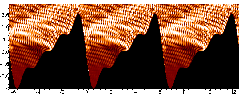
Figure 8: Depiction of the solution of the considered in Table 8 of [6]. This solution resulted from a 1.8 sec. computation, which included the evaluation of the scattered field displayed.

As an additional example we consider Table 5 in [6]. That table presents results for extremely deep sinusoidal gratings with $\lambda=0.05$ and incidence angle $\theta=70^{\circ}$. The corresponding accuracies and computing times produced for those configurations by the present solvers are presented in Table 9. Comparison of the tabulated data shows significant improvements in computing times, by factors of 12 to 25, at the expense of a few digits of accuracy; see Remark 15.

Table 9: Increasingly deep gratings with a fixed period, and with incidence angle $\theta=70^{\circ}$.

$h/\lambda$	$d/\lambda$	$N$	$G^{\textit{qper}}_{0}$ eval.	Init. time	Iter. time	# Iters.	Total time	$\varepsilon$
160	20	800	0.74 sec	1.59 sec	0.08 sec	633	0.84 min	5.9e-08
320	20	1600	1.01 sec	3.31 sec	0.15 sec	1260	3.30 min	5.3e-08
480	20	2400	1.28 sec	4.73 sec	0.26 sec	1881	8.21 min	2.6e-08
640	20	3200	1.59 sec	8.89 sec	0.35 sec	2507	14.88 min	6.1e-08
800	20	4000	1.97 sec	9.96 sec	0.43 sec	3148	22.83 min	8.0e-08

Table 7 in [6], finally, considers increasingly high frequencies while maintaining the other problem parameters fixed: $\theta=45^{\circ}$, $d=1$, $h=2$. A similar picture emerges in this case: the method [6] solves problems with accuracies of the order of 13 to 16 digits, at computing times that are larger than those displayed in Table 10 by factors of 10 to 18.

Table 10: Increasingly high frequencies, with $\theta=45^{\circ}$, $d=1$, $h=2$

$h/\lambda$	$d/\lambda$	$N$	$G^{\textit{qper}}_{0}$ eval.	Init. time	Iter. time	# Iters.	Total time	$\varepsilon$
20	10	200	0.55 sec	0.75 sec	0.01 sec	92	1.62 sec	4.1e-09
40	20	400	1.09 sec	1.51 sec	0.02 sec	167	5.02 sec	1.7e-08
200	100	2000	11.57 sec	13.64 sec	0.25 sec	477	133.67 sec	3.8e-11
400	200	4000	122.78 sec	128.25 sec	1.00 sec	698	824.82 sec	2.4e-09

7 Conclusions

The periodic-scattering solver introduced in this paper provides the first accelerated solver of high-order of accuracy for the solution of problems of scattering by periodic surfaces up to and including Wood frequencies. The algorithm relies on use of an accelerated shifted Green function methodology which reduces operator evaluations to Fast Fourier Transforms, and which, in particular, greatly reduces the required number of evaluations of the shifted quasi-periodic Green function. Significant additional acceleration is obtained by the solver by means of an appropriate application of a dual spectral/spatial approach for evaluation of the shifted Green function—which exploits, when possible, the exponentially fast convergence of the spectral series, and which relies on the high-order-convergent shifted spatial series for points for which the convergence of the spectral series deteriorates. The combined solver is highly efficient: it enables fast and accurate solution of some of the most challenging two-dimensional periodic scattering problems arising in practice. A three-dimensional version of this approach has been found equally effective, and will the subject of a subsequent contribution.

Appendix A Appendix: Convergence and error analysis

An error analysis for the numerical method embodied in equation (53) follows from the standard stability result [19, Th.10.12]. The following lemma establishes the crucial new element necessary to produce a convergence estimate specific to equation (53), namely, an error estimate for the combined smooth windowing and trapezoidal quadrature for the operator $\tilde{D}_{\mathrm{reg}}$ (all other needed estimates can be found in reference [19]). Throughout this section the notations in Section 4.2 are used together with the shorthand $\vec{\mu}=[\mu(x_{1}),\dots,\mu(x_{N})]$ for a given quasi-periodic function $\mu$.

Lemma 1.

Let $d>0$ and $\alpha\geq 0$, and let $\mu$ denote an infinitely differentiable $\alpha$-quasi-periodic function of quasi-period $[0,d]$. Then, $\tilde{D}_{\mathrm{reg}}^{A,\Delta x}[\vec{\mu}](x)$ tends to $\tilde{D}_{\mathrm{reg}}[\mu](x)$, uniformly for $x\in[0,d]$, as $A\to\infty$ and $\Delta x\to 0$. More precisely, we have

$$|\tilde{D}_{\mathrm{reg}}[\mu](x)-\tilde{D}_{\mathrm{reg}}^{A,\Delta x}[\vec{\mu}](x)|\leq E_{p}(\Delta x)^{p}+C_{q}A^{-q}\quad(1\leq i\leq N),$$ (87)

for all positive integers $p$, and with $q=\left\lfloor{\frac{j+1}{2}}\right\rfloor-\frac{1}{2}$ near Wood anomalies, and for all positive integers $q$ away from Wood-anomaly frequencies. Here $C_{q}$ and $E_{p}$ are constants that do not depend on either $A$ or $\Delta x$. We also have the error estimate

$$|\tilde{D}_{\mathrm{reg}}[\mu](x)-\tilde{D}_{\mathrm{reg}}^{\Delta x}[\vec{\mu}](x)|\leq E_{p}(\Delta x)^{p}\quad\mbox{for all }p\in\mathbb{N}.$$ (88)

Proof.

Let us consider the triangle-inequality estimate

$$|\tilde{D}_{\mathrm{reg}}[\mu](x)-\tilde{D}_{\mathrm{reg}}^{A,\Delta x}[\vec{\mu}](x)|\leq|\tilde{D}_{\mathrm{reg}}[\mu](x)-\tilde{D}_{\mathrm{reg}}^{A}[\mu](x)|+|\tilde{D}_{\mathrm{reg}}^{A}[\mu](x)-\tilde{D}_{\mathrm{reg}}^{A,\Delta x}[\vec{\mu}]|.$$ (89)

The first term on the right hand side of this relation admits the bound

$$|\tilde{D}_{\mathrm{reg}}[\mu](x)-\tilde{D}_{\mathrm{reg}}^{A}[\mu](x)|\leq C_{q}A^{-q},$$ (90)

for certain values of $q$, as indicated as follows. For frequencies $\mathrm{k}$ away from Wood anomalies, on one hand, the Green function series converges at a superalgebraic rate as $A\to\infty$ [4], (faster than $A^{-q}$ for any integer $q$), for all integers $j\geq 0$ (including the “unshifted” case $j=0$), and thus so does $\tilde{D}_{\mathrm{reg}}^{A}[\mu]$. In other words, away from Wood anomalies, the bound (90) holds for all positive integers $q$. For frequencies $\mathrm{k}$ up to and including Wood anomalies, on the other hand, reference [4] shows that for a given integer $j\geq 1$, the Green function series enjoys algebraic convergence, with errors of the order of $A^{-q})$ with $q=(j-1)/2$ for $j$ even, and with $q=j/2$ for $j$ odd. It follows that, up to an including Wood anomalies, for a given $j\geq 1$ the bound (90) holds with $q=\left\lfloor{\frac{j+1}{2}}\right\rfloor-\frac{1}{2}$.

Having obtained the estimate (90) for the first term on the right-hand side of (89) under the various frequency regimes, we now turn to the second term on that right-hand side. To estimate this term, we first consider the smooth $2A$-periodic function $F^{A,x}=F^{A,x}(x^{\prime})$ (which, as indicated in Remark 6, coincides with the integrand in equation (43)), and we show that the coefficients

$$F^{A,x}_{n}=\frac{1}{2A}\int_{-A}^{A}F^{A,x}(x^{\prime})e^{-\frac{\pi i}{A}nx^{\prime}}dx^{\prime}$$ (91)

of the Fourier series

$$F^{A,x}(x^{\prime})=\sum_{n=-\infty}^{\infty}F^{A,x}_{n}e^{\frac{\pi i}{A}nx^{\prime}}$$ (92)

converge to zero rapidly and uniformly in $A$ and $x$ as $n\to\infty$. Indeed, using integration by parts $p$ times in (92) we see that

$$|F^{A,x}(x^{\prime})|\leq C^{A,x}_{p}\left(\frac{A}{n}\right)^{p}$$ (93)

where $C^{A,x}_{p}$ is an upper bound for the absolute value of the product of $\pi^{p}$ and the $p$-th derivative of $F^{A,x}(x^{\prime})$ with respect to $x^{\prime}$. But, considering the expression that defines $F^{A,x}(x^{\prime})$, namely, the integrand in (43), we see that the $p$-th order derivative of $F^{A,x}(x^{\prime})$ with respect to $x^{\prime}$ is bounded by a constant which does not depend on $A$ or $x$—since the same is true of each of the four functions in (43) whose products equals $F^{A,x}$. We thus obtain, for each non-negative integer $p$, the bound

$$|F^{A,x}_{n}|<C_{p}\left(\frac{A}{n}\right)^{p},$$ (94)

where the constant $C_{p}$ depends on $p$ only. Since $F^{A,x}(x^{\prime})$ is (a periodic extension of) the integrand in (43), we see that $\tilde{D}_{\mathrm{reg}}^{A}[\mu]$ equals the zero-th order coefficient of $F^{A,x}(x^{\prime})$:

$$\tilde{D}_{\mathrm{reg}}^{A}[\mu]=F^{A,x}_{0}.$$ (95)

The discrete approximation $D_{\mathrm{reg}}^{A,\Delta x}[\vec{\mu}](x)$ in (46), in turn, utilizes in the periodicity interval $[x-A,x+A]$ a number $N_{A}$ of discretization points that satisfies the relations

$$\lfloor A/d\rfloor N\leq N_{A}\leq\lceil A/d\rceil N$$ (96)

where, for a real number $r$, $\lceil r\rceil$ (resp. $\lfloor r\rfloor$) denotes the smallest integer larger than or equal to $r$ (resp. the largest integer smaller than or equal to $r$). For a given period $d$ we clearly have

$$N_{A}=O\left(\frac{A}{N}\right).$$ (97)

As is well known (and easily checked), the $N_{A}$-point discrete trapezoidal-rule quadrature inherent in equation (46) integrates correctly all the non-aliased harmonics in equation (92), and it produces the value one for the aliased harmonics. We thus obtain

$$D_{\mathrm{reg}}^{A,\Delta x}[\vec{\mu}]=\sum_{\ell=-\infty}^{\infty}F^{A,x}_{\ell N_{A}}.$$ (98)

In view of (94), (95) and  (98) it follows that

$$|\tilde{D}_{\mathrm{reg}}^{A}[\mu](x)-\tilde{D}_{\mathrm{reg}}^{A,\Delta x}[\vec{\mu}]|=\left|\sum_{\begin{subarray}{c}\ell=-\infty\\ \ell\neq 0\end{subarray}}^{\infty}F^{A,x}_{\ell N_{A}}\right|\leq C_{p}\left(\frac{A}{N_{A}}\right)^{p}\sum_{\begin{subarray}{c}\ell=-\infty\\ \ell\neq 0\end{subarray}}^{\infty}\ell^{-p}$$ (99)

which, in view of (96) and since $\Delta x\sim 1/N$, for $p\geq 2$ shows that

$$|\tilde{D}_{\mathrm{reg}}^{A}[\mu](x)-\tilde{D}_{\mathrm{reg}}^{A,\Delta x}[\vec{\mu}](x)|\leq E_{p}(\Delta x)^{p}$$ (100)

for some constant $E_{p}$, as desired. The proof is now complete. ∎

References

- [1] T. Arens, S. N. Chandler-Wilde, and J. A. DeSanto. On integral equation and least squares methods for scattering by diffraction gratings. Communications in Computational Physics, 1(6):1010–1042, 2006.
- [2] T. Arens, K. Sandfort, S. Schmitt, and A. Lechleiter. Analysing ewald’s method for the evaluation of Green’s functions for periodic media. IMA Journal of Applied Mathematics, pages 405–431, 2011.
- [3] A. Barnett and L. Greengard. A new integral representation for quasi-periodic scattering problems in two dimensions. BIT Numerical mathematics, 51(1):67–90, 2011.
- [4] O. P. Bruno and B. Delourme. Rapidly convergent quasi-periodic Green function throughout the spectrum - including Wood anomalies. Journal of Computational Physics, January 2014.
- [5] O. P. Bruno and A. G. Fernandez-Lado. Rapidly convergent quasi-periodic Green functions for scattering by arrays of cylinders—including Wood anomalies. Proc. R. Soc. A, 473(2199):20160802, 2017.
- [6] O. P. Bruno and M. Haslam. Efficient high-order evaluation of scattering by periodic surfaces: deep gratings, high frequencies, and glancing incidences. J. Opt. Soc. Am. A, 26(3):658–668, Mar 2009.
- [7] O. P. Bruno and L. Kunyansky. A fast, high-order algorithm for the solution of surface scattering problems: Basic implementation, tests, and applications. Journal of Computational Physics, 169:80–110, 2001.
- [8] O. P. Bruno and M. Maas. Fast 3D Maxwell solvers for bi-periodic structures, including Wood anomalies. In preparation, 2018.
- [9] O. P. Bruno and F. Reitich. Solution of a boundary value problem for the Helmholtz equation via variation of the boundary into the complex domain. Proc. Roy. Soc. Edinburgh Sect. A, 122(3-4):317–340, 1992.
- [10] O. P. Bruno, S. Shipman, C. Turc, and S.Venakides. Superalgebraically convergent smoothly windowed lattice sums for doubly periodic Green functions in three-dimensional space. Proc. R. Soc. A, 2016.
- [11] O. P. Bruno, S. Shipman, C. Turc, and S.Venakides. Three-dimensional quasi-periodic shifted Green function throughout the spectrum–including Wood anomalies. Proc. R. Soc. A, 473(2207):20170242, 2017.
- [12] F. Capolino, D. R. Wilton, and W. A. Johnson. Efficient computation of the 2-D Green’s function for 1-D periodic structures using the Ewald method. IEEE Transactions on Antennas and Propagation, 53(9):2977–2984, 2005.
- [13] R. Chen and J. C. West. Analysis of scattering from rough surfaces at large incidence angles using a periodic-surface moment method. IEEE transactions on geoscience and remote sensing, 33(5):1206–1213, 1995.
- [14] D. Colton and R. Kress. Inverse acoustic and electromagnetic scattering theory, volume 93 of Applied Mathematical Sciences. Springer, second edition, 1997.
- [15] J. DeSanto, G. Erdmann, W. Hereman, and M. Misra. Theoretical and computational aspects of scattering from rough surfaces: one-dimensional surfaces. Waves Random Med., 8(4), 1998.
- [16] K. Ding, L. Tsang, J. Kong, C. Ao, and J. Kong. Scattering of electromagnetic waves, numerical simulation. Remote Sensing, 2001.
- [17] G. H. Golub and C. F. Van Loan. Matrix Computations (3rd Ed.). Johns Hopkins University Press, Baltimore, MD, USA, 1996.
- [18] J. T. Johnson. A numerical study of low-grazing-angle backscatter from ocean-like impedance surfaces with the canonical grid method. IEEE transactions on antennas and propagation, 46(1):114–120, 1998.
- [19] R. Kress. Linear integral equations. Springer-Verlag, New York, third edition, 2014.
- [20] R. Graham L, D. E. Knuth, and O. Patashnik. Concrete mathematics: a foundation for computer science. Addison-Wesley Publishing Company, second edition, 1998.
- [21] N. N. Lebedev. Special functions and their applications. Prentice-Hall, New Jersey, 1965.
- [22] C. M. Linton. The Green’s function for the two-dimensional Helmholtz equation in periodic domains. Journal of Engineering Mathematics, 33(4):377–401, 1998.
- [23] Y. Liu and A. Barnett. Efficient numerical solution of acoustic scattering from doubly-periodic arrays of axisymmetric objects. Journal of Computational Physics, 324:226 – 245, 2016.
- [24] D. Maystre. Rigorous vector theories of diffraction gratings. In E. Wolf, editor, Progress in optics, volume XXI, chapter 1, pages 3–65. Elsevier science publishers, 1983.
- [25] D. Maystre. Theory of Wood’s anomalies. In Plasmonics, pages 39–83. Springer, 2012.
- [26] R. C. McPhedran, G. H. Derrick, and L. C. Botten. Theory of crossed gratings. In Electromagnetic Theory of Gratings, pages 227–276. Springer, 1980.
- [27] Lord Rayleigh. Note on the remarkable case of diffraction spectra described by Prof. Wood. The London, Edinburgh, and Dublin Philosophical Magazine and Journal of Science, 14(79):60–65, 1907.
- [28] Y. Saad and M. Schultz. GMRES: A generalized minimal residual algorithm for solving nonsymmetric linear systems. SIAM Journal on Scientific and Statistical Computing, 7(3):856–869, 1986.
- [29] M. Saillard and G. Soriano. Rough surface scattering at low-grazing incidence: A dedicated model. Radio Science, 46(5), 2011.
- [30] J. E. Stewart and W. S. Gallaway. Diffraction anomalies in grating spectrophotometers. Applied Optics, 1(4):421–430, 1962.
- [31] R. W. Wood. On a remarkable case of uneven distribution of light in a diffraction grating spectrum. The London, Edinburgh, and Dublin Philosophical Magazine and Journal of Science, 4(21):396–402, 1902.