Free-space quantum links under diverse weather conditions

Abstract

Free-space optical communication links are promising channels for establishing secure quantum communication. Here we study the transmission of nonclassical light through a turbulent atmospheric link under diverse weather conditions, including rain or haze. To include these effects, the theory of light transmission through atmospheric links in the elliptic-beam approximation presented by Vasylyev et al. [D. Vasylyev et al., Phys. Rev. Lett. 117, 090501 (2016); arXiv:1604.01373] is further generalized. It is demonstrated, with good agreement between theory and experiment, that low-intensity rain merely contributes additional deterministic losses, whereas haze also introduces additional beam deformations of the transmitted light. Based on these results, we study theoretically the transmission of quadrature squeezing and Gaussian entanglement under these weather conditions.

I Introduction

By the use of modern quantum communication technologies, secret information exchange becomes feasible Skarani . Light is the most attractive candidate for the practical use in quantum communication protocols due to its robustness against the influence of the environment, high bandwidth, and the possibilities of multiplexing information encoding using, e.g., polarization or orbital angular momentum. Recently, quantum communication technologies in free-space channels have developed rapidly. Various experiments have been performed, with distances ranging from intracity Resch ; Martinez ; Peuntinger ; Krenn ; Croal ; Endo to more than 100 km Manderbach ; Fedrizzi2009 ; Yin ; Capraro ; Herbst , which have shown that the atmosphere is a reliable medium for the communication with light exploiting its quantum properties. Moreover, the use of satellite-mediated links Wang ; Bourgoin ; Vallone2015 ; Vallone2016 ; Guenthner ; Liao ; GangRen ; Takenaka paves the way to establish global quantum communication links.

During the propagation through the atmosphere, optical beams undergo random broadening and deformation as well as stochastic deflections as a whole. The major effect comes from the turbulent fluctuations of the refractive index. Moreover, the light beam may be attenuated by backward scattering and absorption. These effects become even more pronounced if the meteorological conditions deviate from what we usually call clear weather. Indeed, under bad weather conditions the optical beam experiences additional broadening, absorption, and backscattering due to random scattering on dust particles, aerosols, and/or precipitations. There exist numerous studies of classical light propagation in turbulent atmosphere in the presence of haze, fog, or rain Hong ; Liu ; Deepak ; Grabner ; Lukin81 ; Yura ; Lukin . Some recent advances were made in the quantum theory of light propagation through atmospheric turbulence Diament ; Perina ; Perina1973 ; Milonni ; Paterson ; Berman ; Semenov ; Vasylyev2012 ; Vasylyev2016 ; Chumak ; Bohmann17 . However, a consistent quantum theory of light propagation in turbulence with the inclusion of random scattering on particles, aerosols, and precipitations has not been developed so far. In contrast to the theory of random scattering of classical light Ishimaru ; Hulst ; IshimaruBook , the quantum theory implies additional constraints, such as commutation rules, so that the classical results cannot be applied in a straightforward manner.

The purpose of our article is to develop a basic quantum theory of light propagation in haze, rain, and turbulence in close relation to experimental observations. To this end, we relate the transmitted quantum state to the initial state at the transmitter site via the input-output relation

$$\hat{a}_{\mathrm{out}}=\sqrt{\eta}\hat{a}_{\mathrm{in}}+\sqrt{1-\eta}\hat{c},$$ (1)

where $\hat{a}_{\mathrm{in(out)}}$ is the input(output) field annihilation operator and $\hat{c}$ is the operator of environmental modes. The transmittance $\eta{\in}[0,1]$ is a random variable that describes the fluctuating-loss channels under study. In terms of the Glauber-Sudarshan $P$ function Glauber ; Sudarshan , the input-output relation (1) reads

$$P_{\rm out}(\alpha)=\int_{0}^{1}{\rm{d}}\eta\mathcal{P}(\eta)\frac{1}{\eta}P_{\rm in}\left(\frac{\alpha}{\sqrt{\eta}}\right).$$ (2)

Here the functions $P_{\rm in}(\alpha)$ and $P_{\rm out}(\alpha)$ are quasiprobability distributions that completely describe the input and output quantum states, respectively. The probability distribution of the transmittance (PDT) $\mathcal{P}(\eta)$ describes fluctuations of the transmission efficiency $\eta$.

In many practical situations one deals with phase-insensitive measurements. Hence, the phase of $\eta$ is not needed in the input-output relation (1). Moreover, even for homodyne measurements one may design the experiment such that the phase fluctuations of the output field amplitude $\hat{a}_{\mathrm{out}}$ can be neglected (see Refs. Elser , Heim for the corresponding experiment and Ref. Toeppel for its theoretical analysis). In general, the atmospheric turbulence and the scattering effects may cause beam deformations, speckles, etc., so a multimode analysis of the transmitted light seems to be necessary. However, the experiments under study can be treated by an effective single-mode scenario (see Appendixes A and C in the Supplemental Material of Ref. Vasylyev2012 ).

Fine properties of fluctuating losses of the channel play a crucial role in free-space quantum communication. Indeed, in many cases one postselects events with the large transmittance Peuntinger ; Semenov2010 ; Erven ; Vallone2015a . In this context the widely-used log-normal distribution Milonni may fail. This happens when fluctuations, which are related to the beam wandering Vasylyev2012 , are significant. In important practical situations, such as in the case of the considered atmospheric link of 1.6 km, both beam wandering and beam-spot distortion contribute in the PDT. This situation can be properly described with the recently proposed elliptic-beam approximation Vasylyev2016 .

In the present article we generalize PDT based on the elliptic-beam approximation Vasylyev2016 , in order to incorporate the influence of random scatterers, such as haze particles and/or raindrops. There are two major effects of random scatterers on the beam: distortion of the beam shape including random deflection of its centroid and random losses due to scattering. We restrict our attention to the theoretical description of the former, while the latter effect is considered only phenomenologically. The theoretical PDTs are compared with the experimental distributions that were measured during daytime and nighttime campaigns in Erlangen with an atmospheric link of $1.6$- km length. The nighttime measurements were performed during the buildup of a hazy turbulent atmosphere, while the atmospheric daytime link was affected by light rainfall. The good agreement between the theoretical and experimental PDTs shows that our generalized elliptic-beam model is capable of describing quantum light propagation through the turbulent atmosphere even under diverse weather conditions.

The paper is organized as follows. In Sec. II we discuss various theoretical aspects such as the input-output relations and the PDT model for atmospheric quantum channels. In Sec. III the experimental setup is discussed and the experimental and theoretical PDTs are compared. The examples of the transfer of quadrature-squeezed and Gaussian-entangled light fields through the turbulent and scattering medium are presented in Sec. IV. A summary is given in Sec. V.

II Model of the turbulent and scattering medium

In the absence of absorption and scattering the fluctuating losses on the receiver site arise mainly due to the finite aperture size of the receiving/detecting system. Let us consider an initially Gaussian beam that propagates along the $z$ axis through the atmosphere. It impinges the circular aperture of radius $a$ placed at the distance $L$ from the transmitter. The atmospheric turbulence leads to random fluctuations of the beam shape and the beam-centroid position. As a result, the transmittance of such a beam through the aperture

$$\eta=\int_{|\boldsymbol{\rho}|^{2}=a^{2}}{\rm{d}}^{2}\boldsymbol{\rho}\left|u(\boldsymbol{\rho},L)\right|^{2},$$ (3)

is a fluctuating parameter cf. Ref. Vasylyev2012 ; Vasylyev2016 . Here $u(\boldsymbol{\rho},L)$ is the beam envelope initially normalized in the transversal plane.

II.1 Light beam in turbulent and scattering media

The envelope function $u(\boldsymbol{\rho},L)$ for an optical beam is obtained by solving the corresponding Helmholtz equation in the paraxial approximation Fante . In this case the norm of the beam is preserved over the whole transmission path and the main effect comes from the losses due to the finite aperture only. Such a technique gives a reasonable result in the case of turbulent atmosphere, when absorption and scattering effects can be neglected. However, these effects become essential for worse weather conditions in the presence of random scatterers, such as dust particles, aerosols, water droplets, etc. For the typical scenario, see Fig. 1.

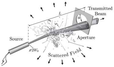
Figure 1: The scheme of optical beam transmission through the turbulent and scattering atmosphere. The beam with initial beam-spot radius $W_{0}$ undergoes random deformations and deflections while propagating in the atmospheric link of length $L$. A part of the radiation field is scattered and absorbed, which is the source of additional extinction losses. The transmitted beam is cut by the circular receiver aperture of radius $a$.

In the presence of random scatterers we can still use Eq. (3) for determining the transmission efficiency. In this case, however, the norm of the beam envelope in the aperture plane can be less than one, due to scattering and absorption losses. While the absorption losses can be included in the paraxial approximation of the Helmholtz equation via the imaginary part of the permittivity, the consistent description of scattering losses requires consideration beyond this approximation.

The resulting electromagnetic field in the scattering media is a superposition of two components: the transmitted beam and the scattered wave. The transmitted beam reaches the plane of the receiver aperture. The amplitude of the scattered wave is proportional to the scattering cross section, which determines the related losses IshimaruBook . Since the norm of the whole electromagnetic wave should be preserved, the transmitted beam appears to be non-normalized.

In this paper we restrict our consideration to the transmitted-beam part of the electromagnetic wave. This part can still be described by using the paraxial approximation. The corresponding approach consistently describes distortions of the beam shape and deflections of the beam centroid by random scatterers. However, it does not yield the value of the corresponding scattering losses since we do not consider the noparaxial part of the scattered field. Hence we use a phenomenological approach for describing these losses. For this purpose we additionally multiply the beam amplitude by the factor $\sqrt{\chi_{\rm ext}}$. The extinction factor $\chi_{\mathrm{ext}}{\in}[0,1]$ is a random variable that describes the absorption and scattering losses. The proper analysis of our experimental data (see Sec. III) shows that the extinction factor can be considered as a nonfluctuating parameter, for the cases of rain and haze in the experimentally studied 1.6 km link.

The solution of the paraxial wave equation together with the extinction factor in the form of a phase approximation of the Huygens-Kirchhoff method Mironov ; Vasylyev2016 is given by

$$u(\boldsymbol{\rho},L) =\sqrt{\chi_{\rm ext}}\int_{\mathbb{R}^{2}}{\rm{d}}^{2}\boldsymbol{\rho}^{\prime}u_{0}(\boldsymbol{\rho}^{\prime})G(\boldsymbol{\rho},\boldsymbol{\rho}^{\prime};L,0).$$ (4)

Here, the Gaussian beam envelope in Eq. (4) at the transmitter plane $z{=}0$ reads

$$u_{0}(\boldsymbol{\rho})=u(\boldsymbol{\rho},z{=}0)=\sqrt{\frac{2}{\pi W_{0}^{2}}}\exp\left[-\frac{1}{W_{0}^{2}}|\boldsymbol{\rho}|^{2}-\frac{ik}{2F}|\boldsymbol{\rho}|^{2}\right],$$ (5)

where $W_{0}$ is the beam-spot radius, $k$ is the optical wave number, and the beam is assumed to be focused at $z{=}F$. The integral kernel in Eq. (4) reads

$$G(\boldsymbol{\rho},\boldsymbol{\rho}^{\prime};z,z^{\prime}) =\frac{k}{2\pi i(z-z^{\prime})}\exp\left[\frac{ik|\boldsymbol{\rho}-\boldsymbol{\rho}^{\prime}|^{2}}{2(z-z^{\prime})}\right]$$

$$\times\exp\left[iS(\boldsymbol{\rho},\boldsymbol{\rho}^{\prime};z,z^{\prime})\right],$$ (6)

where

$$S(\boldsymbol{\rho},\boldsymbol{\rho}^{\prime};z,z^{\prime})=\frac{k}{2}\int\limits_{z^{\prime}}^{z}{\rm{d}}\xi\,\delta\varepsilon\left(\boldsymbol{\rho}\frac{\xi-z^{\prime}}{z-z^{\prime}}+\boldsymbol{\rho}^{\prime}\frac{z-\xi}{z-z^{\prime}},\xi\right)$$ (7)

is the random phase contribution caused by the inhomogeneities of the fluctuating part of the real relative permittivity $\delta\varepsilon(\boldsymbol{\rho},z)$. The random phase has contributions from random scattering, both at turbulent inhomogeneities and at additional random scatterers.

The statistical properties of the light field are affected by the statistical properties of the relative permittivity $\delta\varepsilon$. Note that the latter can be separated in two major contributions,

$$\delta\varepsilon=\delta\varepsilon_{\mathrm{turb}}+\delta\varepsilon_{\mathrm{scat}},$$ (8)

with the parts related to the turbulence $\delta\varepsilon_{\mathrm{turb}}$ and to the random scatterers $\delta\varepsilon_{\mathrm{scat}}$. Here we have assumed that the condition $\delta\varepsilon_{\mathrm{scat}}\gg\delta\varepsilon_{\mathrm{turb}}$ applies. These two parts are also considered to be statistically independent. The correlation function for $\delta\varepsilon$ can be written as Fante

$$\left\langle\delta\varepsilon(\boldsymbol{r}_{1})\delta\varepsilon(\boldsymbol{r}_{2})\right\rangle{=}\int{\rm{d}}^{3}\boldsymbol{K}\,\Phi_{\varepsilon}(\boldsymbol{K})\exp\left[i\boldsymbol{K}{\cdot}(\boldsymbol{r}_{1}-\boldsymbol{r}_{2})\right],$$ (9)

where $\boldsymbol{r}{=}(\boldsymbol{\rho}\quad z)^{T}$, $\boldsymbol{K}{=}(\boldsymbol{\kappa}\quad K_{z})^{T}$ and $\Phi_{\varepsilon}(\boldsymbol{K})$ is the permittivity fluctuation spectrum, which splits as

$$\Phi_{\varepsilon}(\boldsymbol{K})=\Phi_{\varepsilon}^{\mathrm{turb}}(\boldsymbol{K})+\Phi_{\varepsilon}^{\mathrm{scat}}(\boldsymbol{K}),$$ (10)

due to the aforementioned statistical independence of $\delta\varepsilon_{\mathrm{scat}}$ and $\delta\varepsilon_{\mathrm{turb}}$. Using the Markov approximation IshimaruBook ; Fante ; Tatarskii we can further simplify Eq. (9) and write

$$\left\langle\delta\varepsilon(\boldsymbol{r}_{1})\delta\varepsilon(\boldsymbol{r}_{2})\right\rangle{=}2\pi\delta(z_{1}{-}z_{2})\int{\rm{d}}^{2}\boldsymbol{\kappa}\Phi_{\varepsilon}(\boldsymbol{\kappa})e^{i\boldsymbol{\kappa}\cdot(\boldsymbol{\rho}_{1}{-}\boldsymbol{\rho}_{2})},$$ (11)

where $\boldsymbol{\kappa}$ is the transverse wave vector. The Markov approximation is well justified for the turbulent atmosphere Chumak . For the scattering medium, this means that along the propagation direction the scattering on a certain particle is not influenced by the scattering on its neighbor particles Zuev .

For the turbulence part of the spectrum we use the Kolmogorov model Tatarskii ; Fante

$$\Phi_{\varepsilon}^{\mathrm{turb}}(\boldsymbol{\kappa})=0.132C_{n}^{2}|\boldsymbol{\kappa}|^{-\frac{11}{3}},$$ (12)

which is defined in the inertial interval $|\boldsymbol{\kappa}|{\in}[\kappa_{0},\kappa_{\mathrm{m}}]$ with $\kappa_{0}{\sim}1/L_{0}$ and $\kappa_{\mathrm{m}}{\sim}1/l_{0}$. Here $L_{0}$ and $l_{0}$ are the outer and inner scales of turbulence, respectively. The refractive index structure constant $C_{n}^{2}$ characterizes the strength of optical turbulence. In the case of vertical or elevated links, such as ground-satellite links, the dependence of structure constant on altitude should be taken into account.

In Refs. Lukin81 ; Yura it was shown that the spectrum of the correlation function of fluctuations $\delta\varepsilon_{\mathrm{scat}}$ can be written for monodisperse scatterers of size $\mathrm{d}_{\mathrm{scat}}$ as

$$\Phi_{\varepsilon}^{\mathrm{scat}}(\boldsymbol{\kappa})=\frac{2n_{0}}{\pi k^{4}}|f_{0}(\boldsymbol{\kappa};\mathrm{d}_{\mathrm{scat}})|^{2},$$ (13)

where $f_{0}(\boldsymbol{\kappa};\mathrm{d}_{\mathrm{scat}})$ is the amplitude of the wave scattered from a separate particle and $n_{0}$ is the mean number of scattering particles per unit volume. The strict calculations of the amplitude $f_{0}$ can be found in Refs Hulst ; IshimaruBook . For scattering on haze or fog, one uses the Mie scattering theory, whereas the geometric scattering theory is applied for the description of scattering on drizzle and rain.

As shown in Refs. Yura ; Deepak ; Lukin one can approximate $|f_{0}|$ in Eq. (13) in all aforementioned scattering scenarios by Gaussian functions. Equation (13) can be written as

$$\Phi_{\varepsilon}^{\mathrm{scat}}(\boldsymbol{\kappa})=\frac{n_{0}\zeta_{0}^{4}}{8\pi k^{2}}\exp\left[-\zeta_{0}^{2}|\mathbf{\boldsymbol{\kappa}}|^{2}\right].$$ (14)

This approximation means that the fluctuations of the scattering-related relative permittivity has a Gaussian correlation function with the correlation length $2\zeta_{0}$ (see also Appendix C). As was shown in Refs. Yura ; Deepak ; Lukin , the parameter $\zeta_{0}$ is proportional to the particle size $\mathrm{d}_{\mathrm{scat}}$ and for the case of Mie scattering it depends additionally on the light wave number Deepak . We also note that this model resembles the Gaussian phase screen model for the correlation of phases due to random scattering Jakeman1974 ; Jakeman ; Lukin .

II.2 Elliptic-beam model

For many practical purposes we can restrict the effect of the atmosphere on the beam shape to elliptic deformations only. It is also important to include random wandering of the beam centroid into consideration. This is the main idea behind the recently proposed method of the elliptic-beam approximation Vasylyev2016 .

In this model, the PDT, which appears in Eq. (2), is given by

$$\mathcal{P}(\eta){=}\frac{2}{\pi}\int_{\mathbb{R}^{4}}{\rm{d}}^{4}\mathbf{v}\int_{0}^{\pi/2}{\rm{d}}\varphi\,\rho_{G}(\mathbf{v};\boldsymbol{\mu},\boldsymbol{\Sigma})\delta\left(\eta-\eta(\mathbf{v},\varphi)\right).$$ (15)

Here $\eta(\mathbf{v},\varphi)$ is defined by Eq. (3) and is specified for the elliptic beam. Its explicit form is given by Eq. (34) in Appendix A. This is a function of the random vector $\mathbf{v}{=}(x_{0}\quad y_{0}\quad\Theta_{1}\quad\Theta_{2})^{T}$ and the angle $\varphi$ related to the beam-ellipse orientation. The parameters $x_{0}$ and $y_{0}$ correspond to the beam-centroid coordinates and the parameters $\Theta_{i}{=}\ln(W_{i}^{2}/W_{0}^{2})$, $i{=}1,2$, correspond to the ellipse semiaxis $W_{i}$. The distribution function for these parameters, $\rho_{G}(\mathbf{v};\boldsymbol{\mu},\boldsymbol{\Sigma})$, is assumed to be Gaussian with the vector of mean values $\boldsymbol{\mu}$ and the covariance matrix $\boldsymbol{\Sigma}$. The knowledge of parameters $\boldsymbol{\mu}$ and $\boldsymbol{\Sigma}$ enables one to evaluate numerically the integral (15) and therefore to estimate the PDT (for details see Appendix B).

According to the procedure, which is discussed in Ref. Vasylyev2016 , we calculate the values of $\boldsymbol{\mu}$ and $\boldsymbol{\Sigma}$ for the focused beam $L{=}F$ for details see Appendixes C and D. Unlike the consideration in Ref. Vasylyev2016 , here we also take into account the contributions from the spectrum of random scatterers. Specifically, it turns out that these scatterers do not affect the beam wandering, such that the diagonal elements of the matrix $\boldsymbol{\Sigma}$ related to the parameters $x_{0}$ and $y_{0}$ are given by

$$\langle x_{0}^{2}\rangle=\langle y_{0}^{2}\rangle=0.33W_{0}^{2}\sigma_{R}^{2}\Omega^{-\frac{7}{6}},$$ (16)

where $\Omega=\frac{kW_{0}^{2}}{2L}$ is the Fresnel number and

$$\sigma_{R}^{2}=1.23C_{n}^{2}k^{\frac{7}{6}}L^{\frac{11}{6}}$$ (17)

is the Rytov variance Fante ; IshimaruBook which characterizes the strength of phase fluctuations of transmitted light due to scattering on turbulent inhomogeneities. This effect can be explained by the fact that the random scatterers are much smaller than the beam diameter.

The part of the mean vector and the covariance matrix related to the parameters $\Theta_{i}$ are obtained via mean values and the (co)variances of the squared ellipse semiaxes $W_{i}^{2}$,

$$\langle\Theta_{i}\rangle=\ln\left[\frac{\langle W_{i}^{2}\rangle}{W_{0}^{2}\left(1+\frac{\langle(\Delta W_{i}^{2})^{2}\rangle}{\langle W_{i}^{2}\rangle^{2}}\right)^{1/2}}\right],$$ (18)

$$\langle\Delta\Theta_{i}\Delta\Theta_{j}\rangle=\ln\left(1+\frac{\langle\Delta W_{i}^{2}\Delta W_{j}^{2}\rangle}{\langle W_{i}^{2}\rangle\langle W_{j}^{2}\rangle}\right).$$ (19)

These parameters are calculated with the aforementioned technique and read

$$\langle W_{1/2}^{2}\rangle=\frac{W_{0}^{2}}{\Omega^{2}}\Bigl{[}1+\Xi+2.96\sigma_{R}^{2}\Omega^{\frac{5}{9}}\Bigr{]},$$ (20)

$$\langle\Delta W_{i}^{2}\Delta W_{j}^{2}\rangle{=}(2\delta_{ij}{-}0.8)\frac{W_{0}^{4}}{\Omega^{\frac{19}{6}}}\left[1+\Xi\right]\sigma_{R}^{2},$$ (21)

where

$$\Xi=\frac{2}{3}\sigma_{S,\mathrm{scat}}^{2}\frac{W_{0}^{2}}{4\zeta_{0}^{2}}.$$ (22)

is the beam divergence parameter due to the random scattering. In Eq. (22) we have introduced the phase variance of transmitted light due to random scattering as

$$\sigma_{S,\mathrm{scat}}^{2}=\frac{\pi}{4}n_{0}L\zeta_{0}^{2}.$$ (23)

Thus, the random scattering contributes to the beam broadening and to the (co)variances of the beam deformation fluctuations. It is also worth mentioning that in the considered approximation the parameters $\Theta_{i}$ are statistically independent from the beam centroid coordinates $x_{0}$ and $y_{0}$ such that the corresponding covariances vanish (for more details see the Supplemental Material of Ref. Vallone2016 ).

The beam broadening term due to the random scattering in Eq. (20) can be compared with the results obtained within the small-angle approximation of the radiative transfer equation Tam ; Box ; Ishimaru

$$\langle W^{2}_{\rm scat}\rangle=\frac{W_{0}^{2}}{\Omega^{2}}+\frac{2}{3}A\tau L^{2}\overline{\psi^{2}},$$ (24)

where the first term represents beam broadening in free space and the second term is due to random scattering. Here $A$ is the albedo of a single scatterer, i.e., the ratio of the scattering cross section $\sigma_{\rm scat}$ to the extinction cross section $\sigma_{\rm ext}$, $\tau{=}-\ln\chi_{\rm ext}$ is the unitless optical distance Ishimaru , and $\overline{\psi^{2}}$ is the mean square of the scattering angle Hulst ; Box . Comparing Eq. (24) with the first two terms in (20), we obtain the expression for the beam divergence parameter

$$\Xi=\frac{2}{3}\frac{\Omega^{2}}{W_{0}^{2}}A\tau\overline{\psi^{2}}.$$ (25)

This equation relates the model parameters $\zeta_{0}$ and $\sigma_{S,\mathrm{scat}}^{2}$ to the properties of scattering media.

III Experimental results and discussion

We apply the theory to experimental data collected during nighttime and daytime campaigns for various weather conditions. The experimental data were collected in experiments on the free-space distribution of squeezed states of light in an urban free-space channel of 1.6-km length in Erlangen Peuntinger ; Usenko ; Heim2014 . During the measurements, the relative transmission is recorded, which can also be used for atmospheric studies, as it is the case here. The experimental setup is divided into a sender and a receiver. The former consists of a laser (Origami, Onefive GmbH) with central wavelength at 1559-nm emitting pulses with lengths of 200 fs at a repetition rate of 80 MHz. After this light is frequency doubled in a periodically poled lithium niobate crystal (MSHG1550-0.5-0.3, Covesion Ltd.), it is guided through a polarization-maintaining photonic crystal fiber, thereby generating polarization-squeezed states of light that are sent to the receiver. More details on the sender may be found in Peuntinger .

At the receiver the light is collected by an achromatic lens with a diameter of 150-mm and a focal length of ${f{=}800\,\text{mm}}$. The beam is split into two beams by a 50-50 or 90-10 beam splitter for the nighttime measurements and daytime measurement presented here, respectively. Each of the beams is led to a Stokes detection setup consisting of a half waveplate, a polarization beam splitter, and two custom-made pin-diode (S3883, quantum efficiency $\eta_{\mathrm{det}}{=}0.9$, Hamamatsu Photonics K.K.) detectors. The dc output of these detectors is proportional to the intensity of the impinging light and is sampled with a rate of 80-kHz. The typical data acquisition time for the PDTs is on the order of several seconds. The exact durations for the shown data can be found in the captions of Figs. 2, 3, and 5, respectively. Comparing the sum of the four detector outputs with the sent laser power gives the transmission for each sample. The constant losses due to imperfections of all the optical elements in the setup add up to a value of $\eta_{\mathrm{opt}}{=}0.88$.

The nighttime measurements on 24. August 2016 were performed at $00{:}20$ and at $02{:}00$ of local time. During two hours with separate measurements the temperature dropped from 16${}^{\circ}\mathrm{C}$ to 14${}^{\circ}\mathrm{C}$, whereas the relative humidity increased from $85\%$ to $94\%$. The increase of humidity has led to the formation of more dense haze and as a consequence to the reduction of the optical visibility. The corresponding experimental PDTs are obtained by the smooth kernel method Wand and are shown in Figs. 2 and 3.

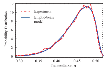
Figure 2: (Color online) Elliptic-beam approximation PDT (solid line) compared with the experimental PDT (dashed line). The measurement was performed at night on 24. August 2016 at 00:20 (local time); the data acquisition time is $12$ s. The other parameters are a wavelength of $780$ nm, the initial spot radius $W_{0}=20$ mm, the aperture radius $a{=}75$ mm, the Rytov parameter $\sigma_{R}^{2}{=}1.78$, the beam divergence parameter due to random scattering $\Xi{=}5$, and the extinction factor $\chi_{\mathrm{ext}}{=}0.51$. The last three parameters are derived from the fitting procedure of the theoretical PDT to the experimental data.

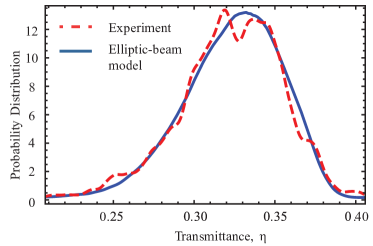
Figure 3: (Color online) Elliptic-beam approximation PDT (solid line) compared with the experimental PDT (dashed line). The measurement was performed at night on 24. August 2016 at 02:00 (local time); the data acquisition time is $9$ s. The estimated from the fit Rytov parameter is $\sigma_{R}^{2}{=}1.05$, the beam divergence parameter $\Xi{=}12$, and $\chi_{\mathrm{ext}}{=}0.40$.

The theoretical curves in Figs. 2 and 3 were calculated by using the elliptic-beam approximation for the PDT [cf. Eq. (15)] by using Monte Carlo methods. We estimated the value for the Rytov parameter $\sigma_{R}^{2}$, the divergence parameter $\Xi$, and the extinction factor $\chi_{\mathrm{ext}}$ with the Pierson’s $\chi^{2}$ criterion Agresti . The increase of humidity between the two measurements led to the increase of the haze particle sizes and the haze number density. The decrease of temperature, on the other hand, reduced the intensity of thermal fluctuations in the atmosphere and hence the strength of optical turbulence. These effects cause a significant change of transmittance statistics. Comparing Fig. 2 with Fig. 3, we see that with an increase of the divergence parameter the PDT becomes more symmetric and resembles a Gaussian distribution. Therefore, the channel presented in Fig. 3 has a smaller probability of attaining high values of transmittance in comparison to the channel in Fig. 2.

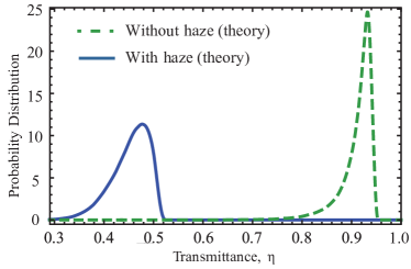
Figure 4: (Color online) Influence of haze on transmission characteristics of the atmospheric channel. The PDT with the inclusion of random scattering due to haze (solid line) is calculated for the same parameters as in Fig. 2, i.e., it corresponds to the experimental data. The PDT without inclusion of haze (dashed line) is theoretically deduced; extinction losses are $\chi_{\mathrm{ext}}{=}0.94$ due to molecular absorption.

In order to demonstrate the impact of haze, in Fig. 4 we show the theoretical PDT from Fig. 2 (solid line) and compare it to the theoretically one deduced when there would not be any haze (dashed line). The extinction of the light signal due to haze shifts the distribution to the smaller values of the transmittance. At the same time, the random scattering broadens the distribution.

The daytime measurement was performed on 08. June 2016 at 11:15 (local time). The meteorological data for this day were the following: $76\%$ humidity, a temperature of $17.6^{\circ}\mathrm{C}$, $3\,\text{mm}/\text{h}$ of mean rain rate during the day. Figure 5 shows the experimental (dashed line) and the theoretical (solid line) PDTs. During the day measurements the atmospheric channel is characterized by a larger value of the Rytov parameter ($\sigma_{R}^{2}=2.88$) in comparison to the night measurements, because of increased turbulence due to thermal convection and wind shear. We have observed that light rain introduces a minor contribution to the phase fluctuation given by Eq. (7) and estimated the divergence parameter as $\Xi=0.2$, i.e., the beam broadening and beam deformation due to rainfall is small. The more pronounced effect of the rainfall is connected with the contribution to the extinction factor $\chi_{\rm ext}$. We have used an empirical formula Zuev ; Rainfall that connects the extinction factor with the path-averaged rainfall intensity $\overline{\mathcal{I}}$ (in mm/h), and propagation distance $L$ (in m) as

$$\chi_{\rm ext}=\exp\bigl{[}-210\,\overline{\mathcal{I}}^{0.74}L\bigr{]}.$$ (26)

The dependence of the extinction coefficient on the water content of precipitations is given in Ref. Mori . In analogy to Fig. 4, Fig. 6 compares the theoretical PDTs with (solid line) and without (dashed line) inclusion of losses due to scattering and absorption by rainfall. One can see that the PDT is shifted to lower values of transmittance and it is narrowed.

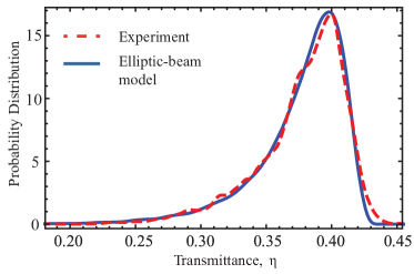
Figure 5: (Color online) Experimental (dashed line) and theoretically fitted (solid line) PDTs for atmospheric quantum channel in the presence of rainfall. The measurement was performed at daytime on 08. June 2016 at 11:15 (local time); the data acquisition time is $14$ s. The estimated Rytov parameter $\sigma_{R}^{2}=2.88$, the beam divergence parameter due to scattering on haze $\Xi{=}0.2$, the path-averaged rain intensity $\overline{\mathcal{I}}{=}3.2\text{mm}/\text{h}$, and $\chi_{\mathrm{ext}}{=}0.43$.

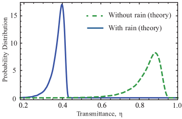
Figure 6: (Color online) Atmospheric channel transmittance distribution with (solid line) and without (dashed line) light rain. The latter PDT includes additional extinction losses $\chi_{\mathrm{ext}}{=}0.94$ due to molecular absorption. The solid line corresponds to the elliptic-beam model fit in Fig. 5, whereas the dashed line is theoretically deduced.

IV Quadrature squeezing and Gaussian entanglement

In order to illustrate the capability of atmospheric channels to preserve nonclassical properties of quantum light, we consider the propagation of quadrature squeezed and Gaussian entangled states through turbulence, rain, and haze. The knowledge of the PDT (15) allows us to analyze the quantum properties of propagating light with the help of the input-output relation (2). Alternatively, one can use directly the input-output relation (1) and the PDT is used for the calculation of moments $\langle\sqrt{\eta}\rangle$, $\langle\eta\rangle$, etc.

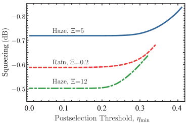
Figure 7: (Color online) Transmitted value of squeezing as a function of postselection threshold $\eta_{\rm min}$. The input light is squeezed to $-2.4$ dB and sent through three atmospheric channels presented in Figs. 2, 3, 5. The predicted behaviors are theoretically evaluated on the basis of the experimental PDTs. The solid line corresponds to the nighttime channel with the Rytov parameter $\sigma_{R}^{2}{=}1.78$, divergence parameter $\Xi{=}5$, extinction losses $\chi_{\mathrm{ext}}{=}0.51$ and mean transmittance $\langle\eta\rangle{=}0.36$. The dashed line corresponds to the rainy daytime channel with $\sigma_{R}^{2}{=}2.88$, $\Xi{=}0.2$, $\chi_{\mathrm{ext}}{=}0.43$, and $\langle\eta\rangle{=}0.29$. The dash-dotted line corresponds to the nighttime channel with haze, $\sigma_{R}^{2}{=}1.05$, $\Xi{=}12$, $\chi_{\mathrm{ext}}{=}0.40$, and $\langle\eta\rangle{=}0.26$. For all curves the additional losses on optical components $\eta_{\ mathrm{opt}}{=}0.88$ and detection efficiency $\eta_{\mathrm{det}}{=}0.9$ are included. All other parameters are the same as in Fig. 2.

The propagation of squeezed light through the turbulent atmosphere has been studied both theoretically Vasylyev2012 and experimentally Peuntinger . It has been shown that the postselection procedure of transmission events with transmittance values greater than the postselection threshold $\eta_{\mathrm{min}}$ yields larger values of the transmitted squeezing Peuntinger ; Heersink . We consider the propagation of quadrature squeezed light ($-2.4$ dB) at $\lambda{=}780$ nm over 1.6 km under different atmospheric conditions. Figure 7 shows the values of squeezing as a function of the postselection threshold for atmospheric channels. The corresponding PDTs are shown in Figs. 2, 3, and 5. The values of transmitted squeezing as well as the maximal postselection threshold values depend on the mean transmittance $\langle\eta\rangle$. The most favorable conditions for squeezing transmission (see the solid line in Fig. 7) are for the night-time measurement with haze and a low value of the divergence parameter $\Xi$ [cf. Eq. (22)]. The stronger optical turbulence during the daytime transmission diminishes the detectable squeezing value (see the dashed line in Fig. 7). At the same time the beam divergence due to scattering plays a minor role here. The dash-dotted line in Fig. 7 shows that the presence of denser haze during the second nighttime measurement contributes to a stronger beam divergence and hence to a smaller efficiency of squeezed light transmission.

As the next example we consider the transmission of Gaussian entanglement of a two-mode squeezed vacuum (TMSV) state in the turbulent atmosphere with haze or rain. Here we closely follow the theoretical analysis of Ref. Bohmann , where it was shown that, in contrast to the channels with deterministic losses, the propagation through the atmosphere with fluctuating transmittance yields certain restrictions on the squeezing degree of the TMSV.

We consider the scenario when one mode of the entangled light fields is sent through the atmospheric channel (field mode $A$), whereas the second one is analyzed locally at the transmitter site (field mode $B$). For the transmitted and detected state we apply the Simon entanglement criterion Simon in the form found in Ref. Shchukin , stating that any two-mode Gaussian state is entangled if and only if

$$\mathcal{W}=\det V^{\mathrm{PT}}<0,$$ (27)

where $V^{\mathrm{PT}}$ is the partial transposition of the matrix

$$V=\left(\begin{array}[]{c c c c}\langle\Delta\hat{a}^{\dagger}\Delta\hat{a}\rangle&\langle\Delta\hat{a}^{\dagger 2}\rangle&\langle\Delta\hat{a}^{\dagger}\Delta\hat{b}\rangle&\langle\Delta\hat{a}^{\dagger}\Delta\hat{b}^{\dagger}\rangle\\ \langle\Delta\hat{a}^{2}\rangle&\langle\Delta\hat{a}\Delta\hat{a}^{\dagger}\rangle&\langle\Delta\hat{a}\Delta\hat{b}\rangle&\langle\Delta\hat{a}\Delta\hat{b}^{\dagger}\rangle\\ \langle\Delta\hat{a}\Delta\hat{b}^{\dagger}\rangle&\langle\Delta\hat{a}^{\dagger}\Delta\hat{b}^{\dagger}\rangle&\langle\Delta\hat{b}^{\dagger}\Delta\hat{b}\rangle&\langle\Delta\hat{b}^{\dagger 2}\rangle\\ \langle\Delta\hat{a}\Delta\hat{b}\rangle&\langle\Delta\hat{a}^{\dagger}\Delta\hat{b}\rangle&\langle\Delta\hat{b}^{2}\rangle&\langle\Delta\hat{b}\Delta\hat{b}^{\dagger}\rangle\end{array}\right).$$ (32)

The matrix $V$ is the second-order matrix of moments of the bosonic creation and annihilation operators of the field modes $A$ and $B$, where $\Delta\hat{x}=\hat{x}-\langle\hat{x}\rangle$ with $\hat{x}=\hat{a},\hat{b}$. The Simon entanglement test $\mathcal{W}_{\rm atm}$ for the state when one mode is transmitted through the atmosphere is obtained by applying the input-output relation (1) to the field mode $A$, i.e., for the operators $\hat{a}$ and $\hat{a}^{\dagger}$. As it was shown in Ref. Bohmann , the entanglement test $\mathcal{W}_{\mathrm{atm}}$ for fluctuating loss channels contains a term that depends on the coherent displacement $|\langle\hat{a}\rangle|$. This feature yields some restrictions on the value of the coherent displacement since for some boundary value $|\langle\hat{a}\rangle|$ the Simon test becomes positive. Similarly, there exists some boundary value of the squeezing parameter $\xi$ above which the Gaussian entanglement is not preserved.

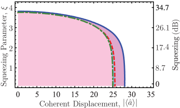
Figure 8: (Color online) Shaded areas represent the regions where the entanglement can be verified by applying the Simon entanglement test, which is a function of the squeezing parameter $\xi$ and of the coherent displacement $|\langle\hat{a}\rangle|$. The solid, dashed, and dash-dotted lines correspond to the bounds of the region where entanglement survives, for the respective channels listed in the caption of Fig. 7.

In Fig. 8 we show the regions where the Gaussian entanglement can be verified for the three atmospheric channels characterized by the PDTs given in Figs. 2, 3, and 5. The boundary values of the coherent amplitude $|\langle\hat{a}\rangle|$ and squeezing parameter $\xi$ are shown by solid, dashed, and dash-dotted lines for the corresponding channels. The boundary values of the squeezing parameter lie beyond the experimentally obtainable squeezing strengths that were obtainable in our experiment. However for long propagation paths this border could be reached already for practically generated TMSV states. This effect therefore should be taken into account when applying TMSV-based quantum protocols for long-distance quantum communication. In Fig. 8 we also see that the presence of random scattering by haze particles shrinks the area where the Gaussian entanglement persists, by reducing the boundary value of the coherent displacement amplitude. Similarly to the case of quadrature squeezing transmission, the particular daytime channel with rain preserves Gaussian entanglement better than the hazy nighttime channels.

V Summary and Conclusions

A quantum state that is transmitted through an atmospheric quantum link experiences fluctuating losses that can spoil or completely destroy its nonclassical properties. Here we studied a realistic intracity free-space quantum channel that has turbulence- and scattering-induced fluctuating losses. Our experimental results show that the transmittance statistics for Gaussian beams strongly depends on the meteorological conditions and can change drastically within a few hours between two measurements. Our theoretical studies explained this situation by taking into account not only the atmospheric turbulence but also the random scattering on haze particles or on raindrops. Using the elliptic-beam model for the beam transmitted through the atmosphere and impinging on the receiver aperture, we have shown that random scattering on haze particles contributes to the beam broadening and beam shape deformation. The action of rain shows minor beam broadening and deformation effects, but it contributes to the extinction losses.

We have studied the transmission of quadrature squeezing and Gaussian entanglement through realistic quantum optical links with turbulence, haze and rain. We have found that a detectable squeezing value depends on the propagation conditions and it is strongly affected by random scattering. For example, the daytime transmission in rain preserves squeezing better than the nighttime transmission in haze, despite the fact that the optical turbulence is considerably stronger during the day. Similar effects have been found by analyzing the transmission of Gaussian entanglement through atmosphere. Random scattering on haze particles constricts the area of the values of the squeezing parameter and coherent amplitude, for which entanglement is verified. The obtained results may be useful for the analysis of quantum communication protocols in intracity atmospheric channels under diverse weather and day-time conditions.

Appendix A Aperture transmittance

In this appendix we remind the reader of some details on the elliptic-beam model for the PDT Vasylyev2016 . We choose the coordinate system such that the $z$ axis is aligned along the line that connects the centers of transmitter and receiver apertures. The distance between the transmitter and the receiver aperture plane is $z{=}L$. The transmission efficiency of an elliptic beam through a circular aperture of radius $a$ is given by Eq. (3), where the beam intensity at the aperture plane is assumed to have the Gaussian form

$$|u(\boldsymbol{\rho},L)|^{2}{=}\frac{2\chi_{\mathrm{ext}}}{\pi\sqrt{\det\mathbf{S}}}\exp\Bigl{[}-2(\boldsymbol{\rho}{-}\boldsymbol{\rho}_{0})^{T}\mathbf{S}^{-1}(\boldsymbol{\rho}{-}\boldsymbol{\rho}_{0})\Bigr{]}.$$ (33)

Here, $\boldsymbol{\rho}{=}(x\quad y)^{T}$ is the transverse coordinate, $\boldsymbol{\rho}_{0}{=}(\rho_{0}\cos\phi_{0}\quad\rho_{0}\sin\phi_{0})^{T}$ is the beam centroid position coordinate, $\mathbf{S}$ is the real, symmetric, positive-definite spot-shape matrix, and $\chi_{\rm ext}$ is the extinction factor due to absorption and scattering. In general, the intensity (33) has an elliptic profile. Applying the rotation by a certain angle $\varphi$, we can bring the spot shape matrix into diagonal form with the elements $W_{i}^{2}$, $i{=}1,2$, which are the squared major semi-axes of the ellipse.

Substituting Eq. (33) in Eq. (3), one can show that the transmission efficiency can be approximated by the following expression (cf. Ref. Vasylyev2016 ):

$$\eta=\eta_{0}\exp\left\{-\left[\frac{\rho_{0}/a}{R\left(\frac{2}{W_{\rm eff}(\varphi-\phi_{0})}\right)}\right]^{\lambda\left(\frac{2}{W_{\rm eff}(\varphi-\phi_{0})}\right)}\right\}.$$ (34)

Here the maximal transmittance for a centered beam,

$$\eta_{0} =1{-}{\rm{I}}_{0}\left(a^{2}\frac{W_{1}^{2}-W_{2}^{2}}{W_{1}^{2}W_{2}^{2}}\right)e^{-a^{2}\frac{W_{1}^{2}+W_{2}^{2}}{W_{1}^{2}W_{2}^{2}}}$$

$$-2\Bigl{[}1{-}e^{-\frac{a^{2}}{2}\Bigl{(}\frac{1}{W_{1}}{-}\frac{1}{W_{2}}\Bigr{)}}\Bigr{]}$$ (35)

$$\times\exp\left[-\left\{\frac{\frac{(W_{1}+W_{2})^{2}}{|W_{1}^{2}-W_{2}^{2}|}}{R\left(\frac{1}{W_{1}}-\frac{1}{W_{2}}\right)}\right\}^{\lambda\left(\frac{1}{W_{1}}-\frac{1}{W_{2}}\right)}\right]$$

is a function of the two eigenvalues $W_{i}^{2}$ of the spot-shape matrix $\mathbf{S}$ and ${\rm{I}}_{n}(x)$ is the modified Bessel function of $n$-th order. The shape $\lambda$ and scale $R$ functions are given by

$$\lambda(\xi) =2a^{2}\xi^{2}\frac{e^{-a^{2}\xi^{2}}{\rm{I}}_{1}\left(a^{2}\xi^{2}\right)}{1-\exp\left[-a^{2}\xi^{2}\right]{\rm{I}}_{0}\left(a^{2}\xi^{2}\right)}$$

$$\times\left[\ln\left(2\frac{1-\exp\left[-\frac{1}{2}a^{2}\xi^{2}\right]}{1-\exp\left[-a^{2}\xi^{2}\right]{\rm{I}}_{0}\left(a^{2}\xi^{2}\right)}\right)\right]^{-1},$$ (36)

$$R(\xi)=\left[\ln\left(2\frac{1-\exp\left[-\frac{1}{2}a^{2}\xi^{2}\right]}{1-\exp\left[-a^{2}\xi^{2}\right]{\rm{I}}_{0}\left(a^{2}\xi^{2}\right)}\right)\right]^{-\frac{1}{\lambda(\xi)}},$$ (37)

where the effective squared spot radius

$$W_{\rm eff}^{2}(\varphi-\phi_{0})=4a^{2}\Bigl{[}\mathcal{W}\Bigl{(}\frac{4a^{2}}{W_{1}W_{2}}e^{2a^{2}\left(\frac{1}{W_{1}^{2}}+\frac{1}{W_{2}^{2}}\right)}\Bigr{.}\Bigr{.}$$ (38)

$$\qquad\times\Bigl{.}\Bigl{.}e^{a^{2}\left(\frac{1}{W_{1}^{2}}-\frac{1}{W_{2}^{2}}\right)\cos(2\varphi-2\phi_{0})}\Bigr{)}\Bigr{]}^{-1}$$ (39)

is expressed with the help of the Lambert function $\mathcal{W}(x)$ (cf. Ref. Corless ). Thus, the elliptic beam transmittance (34) is a function of the random variables $\boldsymbol{\rho}_{0}=(x_{0}\quad y_{0})^{T}$, $W_{1}^{2}$, $W_{2}^{2}$, and $\phi{=}\varphi-\phi_{0}$; or, alternatively, of the variables $\boldsymbol{\rho}_{0}$, $\Theta_{1}$, $\Theta_{2}$, and $\phi$, where

$$W_{i}^{2}=W_{0}^{2}\exp{\Theta_{i}},$$ (40)

with $W_{0}^{2}$ being the beam spot radius at the transmitter.

Appendix B Evaluation of the PDT

In this appendix we discuss how to numerically evaluate the PDT in Eq. (15), based on the knowledge of relevant atmospheric and beam parameters. To this end one should proceed with the following steps.

1. One calculates the components of covariance matrix $\boldsymbol{\Sigma}$ and mean values $\boldsymbol{\mu}$ of the random vector $\textbf{v}=(x_{0}\quad y_{0}\quad\Theta_{1}\quad\Theta_{2})^{\mathrm{T}}$ using Eqs. (16) and (18)–(21) and knowledge about the corresponding beam, aperture parameters, atmospheric structure constant $C_{n}^{2}$, and beam divergence parameter $\Xi$. We note, however, that the analytical results (16), (20), and (21) were obtained in the asymptotic case of weak-to-moderate turbulence. The elliptic-beam approximation in the present form does not work for arbitrary channels.

2. Then the numerical integration in Eq. (15) can be performed within a Monte Carlo method. For this purpose one should simulate the $N$ values of the vector v and the angle $\phi$. The angle $\phi$ is assumed to be uniformly distributed in the interval $[0,\pi/2]$. The simulated values of v and $\phi$ are substituted into Eq. (34) by taking into account that $\phi{=}\varphi{-}\phi_{0}$. Finally, the obtained transmittances are multiplied with the extinction factor $\chi_{\mathrm{ext}}$ yielding $N$ values of atmospheric transmittance $\chi_{\mathrm{ext}}\eta(\textbf{v}_{i},\phi_{i})$, $i{=}1,...,N$. The corresponding PDT can be visualized using the simulated values of transmittance via histograms or using the techniques of smooth kernels Wand .

3. In most practical situations the knowledge of mean value of some quantity that is function of transmittance $\langle f(\eta)\rangle$ is needed. Such a quantity is estimated from the simulated values of transmittance as

   $$\langle f(\eta)\rangle\approx\frac{1}{N}\sum_{i=1}^{N}f(\chi_{\mathrm{ext}}\eta(\textbf{v}_{i},\phi_{i})).$$ (41)

   where $\eta(\textbf{v}_{i},\phi_{i})$ is obtained from Eq. (34). For example, one can obtain the first two moments of the atmospheric transmittance as

   $$\langle\eta\rangle\approx\chi_{\mathrm{ext}}\frac{1}{N}\sum_{i=1}^{N}\eta(\textbf{v}_{i},\phi_{i}),$$ (42)

   $$\langle\eta^{2}\rangle\approx\chi_{\mathrm{ext}}^{2}\frac{1}{N}\sum_{i=1}^{N}\eta^{2}(\textbf{v}_{i},\phi_{i}).$$ (43)

Appendix C Statistical parameters for the elliptic beam and optical field correlations

The vector $\mathbf{v}=(x_{0}\quad y_{0}\quad\Theta_{1}\quad\Theta_{2})^{T}$ is a Gaussian random vector. The angle variable $\phi$ is assumed to be uniformly distributed in the interval $[0,\frac{\pi}{2}]$. The reference frame is chosen such that $\langle x_{0}\rangle=\langle y_{0}\rangle=0$ and

$$\langle x_{0}^{2}\rangle=\langle y_{0}^{2}\rangle=\frac{1}{\chi_{\mathrm{ext}}^{2}}\int_{\mathbb{R}^{4}}{\rm{d}}^{2}\boldsymbol{\rho}_{1}{\rm{d}}^{2}\boldsymbol{\rho}_{2}\,x_{1}x_{2}\Gamma_{4}(\boldsymbol{\rho}_{1},\boldsymbol{\rho}_{2};L),$$ (44)

where $\Gamma_{4}(\boldsymbol{\rho}_{1},\boldsymbol{\rho}_{2};z){=}\langle u^{\ast}(\boldsymbol{\rho}_{1},z)u(\boldsymbol{\rho}_{1},z)u^{\ast}(\boldsymbol{\rho}_{2},z)u(\boldsymbol{\rho}_{2},z)\rangle$ is the fourth-order field-correlation function. The means and (co)variances of $\Theta_{i}$ are expressed via the means and (co)variances of $W_{i}^{2}$ by Eqs. (18) and (19), respectively. Under the assumptions of Gaussianity and isotropy (for details see the Supplemental Material of Ref. Vasylyev2016 ) the means and (co)variances of $W_{i}^{2}$ read

$$\langle W_{1/2}^{2}\rangle=4\left[\frac{1}{\chi_{\mathrm{ext}}}\int_{\mathbb{R}^{2}}{\rm{d}}^{2}\boldsymbol{\rho}\,x^{2}\Gamma_{2}(\boldsymbol{\rho};L)-\langle x_{0}^{2}\rangle\right],$$ (45)

$$\langle\Delta W_{i}^{2}\Delta W_{j}^{2}\rangle={-}\frac{8}{\chi_{\mathrm{ext}}^{2}}\Biggl{\{}2\left(\int_{\mathbb{R}^{2}}{\rm{d}}^{2}\boldsymbol{\rho}\,x^{2}\Gamma_{2}(\boldsymbol{\rho};L)\right)^{2}\Biggr{.}$$

$${-}\int_{\mathbb{R}^{4}}{\rm{d}}^{2}\boldsymbol{\rho}_{1}{\rm{d}}^{2}\boldsymbol{\rho}_{2}\bigl{[}x_{1}^{2}x_{2}^{2}(4\delta_{ij}{-}1)-x_{1}^{2}y_{2}^{2}(4\delta_{ij}{-}3)\bigr{]}$$

$$\qquad{\times}\Gamma_{4}(\boldsymbol{\rho}_{1},\boldsymbol{\rho}_{2};L)\Biggr{\}}-16\left[4\delta_{ij}-1\right]\langle x_{0}^{2}\rangle^{2},$$ (46)

where we have also used the second-order field-correlation function $\Gamma_{2}(\boldsymbol{\rho};z){=}\langle u^{\ast}(\boldsymbol{\rho},z)u(\boldsymbol{\rho},z)\rangle$.

For the calculation of the field-correlation functions $\Gamma_{2}$ and $\Gamma_{4}$ in Eqs. (44)-(C) we use the expression (4) for the field envelope $u(\boldsymbol{\rho},z)$. Substituting Eq. (4) in the second- and fourth-order field correlation functions and performing the statistical averaging one gets

$$\Gamma_{2}(\boldsymbol{\rho};L)=\chi_{\mathrm{ext}}\int_{\mathbb{R}^{4}}{\rm{d}}^{2}\boldsymbol{\rho}_{1}^{\prime}{\rm{d}}^{2}\boldsymbol{\rho}_{2}^{\prime}\,u_{0}(\boldsymbol{\rho}^{\prime}_{1})u^{\ast}_{0}(\boldsymbol{\rho}_{2}^{\prime})G_{0}(\boldsymbol{\rho},\boldsymbol{\rho}^{\prime}_{1};L,0)$$

$${\times}G_{0}^{\ast}(\boldsymbol{\rho},\boldsymbol{\rho}^{\prime}_{2};L,0)\left\langle\exp\left[iS(\boldsymbol{\rho},\boldsymbol{\rho}_{1}^{\prime};L,0){-}iS(\boldsymbol{\rho},\boldsymbol{\rho}_{2}^{\prime};L,0)\right]\right\rangle,$$ (47)

$$\Gamma_{4}(\boldsymbol{\rho}_{1},\boldsymbol{\rho}_{2};L){=}\eta_{\mathrm{ext}}^{2}\int_{\mathbb{R}^{8}}{\rm{d}}^{2}\boldsymbol{\rho}_{1}^{\prime}...{\rm{d}}^{2}\boldsymbol{\rho}_{4}^{\prime}\,u_{0}(\boldsymbol{\rho}^{\prime}_{1})u^{\ast}_{0}(\boldsymbol{\rho}_{2}^{\prime})u_{0}(\boldsymbol{\rho}^{\prime}_{3})$$

$$\times u^{\ast}_{0}(\boldsymbol{\rho}_{4}^{\prime})G_{0}(\boldsymbol{\rho}_{1},\boldsymbol{\rho}^{\prime}_{1};L,0)G_{0}^{\ast}(\boldsymbol{\rho}_{1},\boldsymbol{\rho}^{\prime}_{2};L,0)G_{0}(\boldsymbol{\rho}_{2},\boldsymbol{\rho}^{\prime}_{3};L,0)$$

$$\times G_{0}^{\ast}(\boldsymbol{\rho}_{2},\boldsymbol{\rho}^{\prime}_{4};L,0)\left\langle\exp\left[iS(\boldsymbol{\rho}_{1},\boldsymbol{\rho}^{\prime}_{1};L,0){-}iS(\boldsymbol{\rho}_{1},\boldsymbol{\rho}^{\prime}_{2};L,0)\right.\right.$$

$$\qquad\qquad\qquad\left.\left.+iS(\boldsymbol{\rho}_{2},\boldsymbol{\rho}^{\prime}_{3};L,0){-}iS(\boldsymbol{\rho}_{2},\boldsymbol{\rho}^{\prime}_{4};L,0)\right]\right\rangle,$$ (48)

with

$$G_{0}(\boldsymbol{\rho},\boldsymbol{\rho}^{\prime};z,z^{\prime})=\frac{k}{2\pi i(z-z^{\prime})}\exp\left[\frac{ik|\boldsymbol{\rho}-\boldsymbol{\rho}^{\prime}|^{2}}{2(z-z^{\prime})}\right].$$ (49)

Assuming that the relative permittivity $\delta\varepsilon$ is a Gaussian stochastic field, we can rewrite Eqs. (C) and (C) as

$$\Gamma_{2}(\boldsymbol{\rho};L)=\chi_{\mathrm{ext}}\int_{\mathbb{R}^{4}}{\rm{d}}^{2}\boldsymbol{\rho}_{1}^{\prime}{\rm{d}}^{2}\boldsymbol{\rho}_{2}^{\prime}\,u_{0}(\boldsymbol{\rho}^{\prime}_{1})u^{\ast}_{0}(\boldsymbol{\rho}_{2}^{\prime})G_{0}(\boldsymbol{\rho},\boldsymbol{\rho}^{\prime}_{1};L,0)$$

$$\quad\times G_{0}^{\ast}(\boldsymbol{\rho},\boldsymbol{\rho}^{\prime}_{2};L,0)\exp\Bigl{[}-\frac{1}{2}\mathcal{D}_{S}(0,\boldsymbol{\rho}_{1}^{\prime}{-}\boldsymbol{\rho}_{2}^{\prime})\Bigr{]},$$ (50)

$$\Gamma_{4}(\boldsymbol{\rho}_{1},\boldsymbol{\rho}_{2};L){=}\chi_{\mathrm{ext}}^{2}\int_{\mathbb{R}^{8}}\!\!{\rm{d}}^{2}\boldsymbol{\rho}_{1}^{\prime}...{\rm{d}}^{2}\boldsymbol{\rho}_{4}^{\prime}\,u_{0}(\boldsymbol{\rho}^{\prime}_{1})u^{\ast}_{0}(\boldsymbol{\rho}_{2}^{\prime})u_{0}(\boldsymbol{\rho}^{\prime}_{3})u^{\ast}_{0}(\boldsymbol{\rho}_{4}^{\prime})$$

$$\times G_{0}(\boldsymbol{\rho}_{1},\boldsymbol{\rho}^{\prime}_{1};L,0)G_{0}^{\ast}(\boldsymbol{\rho}_{1},\boldsymbol{\rho}^{\prime}_{2};L,0)G_{0}(\boldsymbol{\rho}_{2},\boldsymbol{\rho}^{\prime}_{3};L,0)$$

$$\times G_{0}^{\ast}(\boldsymbol{\rho}_{2},\boldsymbol{\rho}^{\prime}_{5};L,0)\exp\Biggl{[}-\frac{1}{2}\Bigl{\{}\mathcal{D}_{S}(0,\boldsymbol{\rho}_{1}^{\prime}{-}\boldsymbol{\rho}^{\prime}_{2})+\mathcal{D}_{S}(0,\boldsymbol{\rho}_{3}^{\prime}{-}\boldsymbol{\rho}^{\prime}_{4})$$

$$\qquad\qquad-\sum_{\begin{subarray}{c}i=1,2\\ j=3,4\end{subarray}}(-1)^{i+j}\mathcal{D}_{S}(\boldsymbol{\rho}_{1}{-}\boldsymbol{\rho}_{2},\boldsymbol{\rho}_{i}^{\prime}{-}\boldsymbol{\rho}^{\prime}_{j})\Bigr{\}}\Biggr{]},$$ (51)

where

$$\mathcal{D}_{S}(\boldsymbol{\rho}_{k}{-}\boldsymbol{\rho}_{l},\boldsymbol{\rho}_{k}^{\prime}{-}\boldsymbol{\rho}_{l}^{\prime})$$

$$\qquad=\left\langle\left[S(\boldsymbol{\rho}_{k},\boldsymbol{\rho}_{k}^{\prime};z,z^{\prime})-S(\boldsymbol{\rho}_{l},\boldsymbol{\rho}_{l}^{\prime};z,z^{\prime})\right]^{2}\right\rangle$$ (52)

is the structure function of the phase fluctuations.

Using Eq. (7) and the Markovian approximation (cf., e.g., Ref Fante ), we obtain for $z^{\prime}{=}0$, and $z{=}L$,

$$\mathcal{D}_{S}(\boldsymbol{\rho}_{k}{-}\boldsymbol{\rho}_{l},\boldsymbol{\rho}_{k}^{\prime}{-}\boldsymbol{\rho}_{l}^{\prime})$$

$$=\frac{k^{2}L^{2}}{4}\int_{0}^{1}{\rm{d}}\xi\Bigl{\langle}\Bigl{\{}\delta\varepsilon\left(\boldsymbol{\rho}_{k}\xi{+}\boldsymbol{\rho}^{\prime}_{k}[1{-}\xi],\xi\right)$$

$$\qquad\qquad\qquad-\delta\varepsilon\left(\boldsymbol{\rho}_{l}\xi{+}\boldsymbol{\rho}_{l}^{\prime}[1{-}\xi],\xi\right)\Bigr{\}}^{2}\Bigr{\rangle},$$ (53)

i.e., we assume that turbulent inhomogeneities as well as random scatterers represented by the relative permittivity $\delta\varepsilon$ are $\delta$ correlated in the $z$ direction. In this case the structure function (C) can be written in terms of the permittivity fluctuation spectrum $\Phi_{\varepsilon}(\boldsymbol{\kappa})$ as

$$\mathcal{D}_{S}(\boldsymbol{\rho},\boldsymbol{\rho}^{\prime})=\frac{\pi}{2}k^{2}L\int_{0}^{1}{\rm{d}}\xi\int_{\mathbb{R}^{2}}{\rm{d}}^{2}\boldsymbol{\kappa}\,\Phi_{\varepsilon}(\boldsymbol{\kappa})$$

$$\times\Bigl{(}1-\exp\bigl{\{}i\boldsymbol{\kappa}{\cdot}\left[\boldsymbol{\rho}\xi{+}\boldsymbol{\rho}^{\prime}(1{-}\xi)\right]\bigr{\}}\Bigr{)},$$ (54)

where, due to the Markovian approximation, the spectrum depends on the reduced vector $\boldsymbol{\kappa}$, which is related to the vector $\mathbf{K}$ in Eq. (10) as $\mathbf{K}=(\kappa_{x}\quad\kappa_{y}\quad 0)^{T}$. Moreover, taking into account that the spectrum splits into two parts [cf. Eq. (10)], we can write

$$\mathcal{D}_{S}=\mathcal{D}_{S}^{\mathrm{turb}}+\mathcal{D}_{S}^{\mathrm{scat}},$$ (55)

i.e. the phase structure function also splits into turbulent- and random scattering-induced contributions.

Based on the Kolmogorov turbulence spectrum (12) and the proposed Gaussian spectrum (14) for random scatterers, we obtain for the corresponding structure functions

$$\mathcal{D}_{S}^{\rm turb}(\boldsymbol{\rho},\boldsymbol{\rho}^{\prime})=2.4\sigma_{R}^{2}k^{\frac{5}{6}}L^{-\frac{5}{6}}\int_{0}^{1}{\rm{d}}\xi\left|\boldsymbol{\rho}\xi+\boldsymbol{\rho}^{\prime}(1-\xi)\right|^{\frac{5}{3}},$$ (56)

$$\mathcal{D}_{S}^{\mathrm{scat}}(\boldsymbol{\rho},\boldsymbol{\rho}^{\prime})=2\sigma_{S,\mathrm{scat}}^{2}\int_{0}^{1}{\rm{d}}\xi$$ (57)

$$\times\Bigl{\{}1-\exp\left[-\Bigl{|}(\boldsymbol{\rho}_{1}{-}\boldsymbol{\rho}_{2})\xi{+}(\boldsymbol{\rho}_{1}^{\prime}{-}\boldsymbol{\rho}_{2}^{\prime})(1{-}\xi)\Bigr{|}^{2}/4\zeta_{0}^{2}\right]\Bigr{\}}.$$

Here, the Rytov variance $\sigma_{R}^{2}$ is given by Eq. (17), $\zeta_{0}$ is the transversal correlation length for random scatterers, and $\sigma_{S,\mathrm{scat}}^{2}$ is the corresponding phase variance given by Eq. (23). For weather conditions with high visibility (haze and thin fog) the correlation length $\zeta_{0}$ is large. In this case the phase structure function reads

$$\mathcal{D}_{S}^{\mathrm{scat}}(\boldsymbol{\rho},\boldsymbol{\rho}^{\prime}){=}\frac{\sigma_{S,\mathrm{scat}}^{2}}{2\zeta_{0}^{2}}\int_{0}^{1}{\rm{d}}\xi\left|\boldsymbol{\rho}\xi{+}\boldsymbol{\rho}^{\prime}(1{-}\xi)\right|^{2},$$ (58)

and it is a quadratic function of its arguments.

We substitute Eqs. (56) and (58) into Eqs. (C) and (C) and perform the corresponding integration. This results in the expressions for the field correlation functions

$$\Gamma_{2}(\boldsymbol{\rho}) =\chi_{\mathrm{ext}}\frac{\Omega^{2}}{\pi^{2}W_{0}^{4}}\int_{\mathbb{R}^{2}}{\rm{d}}^{2}\boldsymbol{\rho}^{\prime}e^{-\frac{\gamma^{2}}{2W_{0}^{2}}|\boldsymbol{\rho}^{\prime}|^{2}-2i\frac{\Omega}{W_{0}}\boldsymbol{\rho}\cdot\boldsymbol{\rho}^{\prime}}$$

$$\times\exp\Bigl{[}-\frac{1}{2}\mathcal{D}_{S}^{\mathrm{turb}}(0,\boldsymbol{\rho}^{\prime})\Bigr{]},$$ (59)

$$\Gamma_{4}(\boldsymbol{\rho}_{1},\boldsymbol{\rho}_{2})=\chi_{\mathrm{ext}}^{2}\frac{4\Omega^{4}}{\pi^{5}W_{0}^{10}}\int_{\mathbb{R}^{6}}{\rm{d}}^{2}\boldsymbol{\rho}^{\prime}_{1}{\rm{d}}^{2}\boldsymbol{\rho}^{\prime}_{2}{\rm{d}}^{2}\boldsymbol{\rho}^{\prime}_{3}$$

$$\times e^{-\frac{1}{W_{0}^{2}}\bigl{(}|\boldsymbol{\rho}_{1}^{\prime}|^{2}+|\boldsymbol{\rho}_{2}^{\prime}|^{2}+\gamma^{2}|\boldsymbol{\rho}_{3}^{\prime}|^{2}\bigr{)}}e^{2i\frac{\Omega}{W_{0}^{2}}\boldsymbol{\rho}_{1}^{\prime}\cdot\boldsymbol{\rho}_{2}^{\prime}}$$

$$\qquad\times e^{-2i\frac{\Omega}{W_{0}^{2}}\bigl{[}(\boldsymbol{\rho}_{1}-\boldsymbol{\rho}_{2})\cdot\boldsymbol{\rho}_{2}^{\prime}+(\boldsymbol{\rho}_{1}{+}\boldsymbol{\rho}_{2})\cdot\boldsymbol{\rho}_{3}^{\prime}\bigr{]}}$$ (60)

$$\times\exp\Bigl{[}-\frac{1}{2}\sum_{j=1,2}\Bigl{\{}\mathcal{D}_{S}^{\mathrm{turb}}(\boldsymbol{\rho}_{1}{-}\boldsymbol{\rho}_{2},\boldsymbol{\rho}_{1}^{\prime}{+}(-1)^{j}\boldsymbol{\rho}_{3}^{\prime})$$

$$+\mathcal{D}_{S}^{\mathrm{turb}}(0,\boldsymbol{\rho}_{2}^{\prime}{+}(-1)^{j}\boldsymbol{\rho}_{3}^{\prime}){-}\mathcal{D}_{S}^{\mathrm{turb}}(\boldsymbol{\rho}_{1}{-}\boldsymbol{\rho}_{2},\boldsymbol{\rho}_{1}^{\prime}{+}(-1)^{j}\boldsymbol{\rho}_{2}^{\prime})\Bigr{\}}\Bigr{]}.$$

Here

$$\gamma^{2}=1+\Omega^{2}\left(1-\frac{L}{F}\right)^{2}+\frac{2}{3}\sigma_{S,\mathrm{scat}}^{2}\frac{W_{0}^{2}}{4\zeta_{0}^{2}}$$ (61)

is the generalized beam diffraction parameter that includes the contribution from random scattering and $\Omega$ is the Fresnel number of the transmitter aperture.

Appendix D Beam wandering and beam shape distortion in the presence of random scatterers and turbulence

In this appendix we derive the statistical characteristics of the elliptic beam taking into account the presence of random scatterers. The derivations follow closely the calculations given in the Supplemental Material of Ref. Vasylyev2016 .

D.1 Beam wandering

The main contribution to beam wandering comes from large turbulent eddies located close to the beam transmitter Andrews . This allows us to replace the integral along the propagation path in Eq. (C) with its value at the transmitter aperture plane Kon ; Klyatskin ; MironovBook , i.e.,

$$\int_{z^{\prime}}^{z}{\rm{d}}\xi f(\xi)\approx(z-z^{\prime})f(z^{\prime}).$$ (62)

The phase structure function then reduces to

$$\mathcal{D}_{S}(\boldsymbol{\rho},\boldsymbol{\rho}^{\prime})=\mathcal{D}_{S}^{\mathrm{turb}}(\boldsymbol{\rho},\boldsymbol{\rho}^{\prime})=2.4\sigma_{R}^{2}k^{\frac{5}{6}}L^{-\frac{5}{6}}|\boldsymbol{\rho}^{\prime}|^{\frac{5}{3}}.$$ (63)

Here we have set $\mathcal{D}_{S}^{\mathrm{scat}}(\boldsymbol{\rho},\boldsymbol{\rho}^{\prime}){=}0$, which is justified if the characteristic sizes of random scatterers are less than the characteristic sizes of eddies contributing to beam wandering.

Substituting Eq. (C) into (44), we obtain for the beam wandering variance the expression

$$\langle x_{0}^{2}\rangle{=}\frac{4\Omega^{4}}{\pi^{5}W_{0}^{10}}\int_{\mathbb{R}^{8}}{\rm{d}}^{2}\widetilde{\mathbf{R}}\,{\rm{d}}^{2}\widetilde{\boldsymbol{\rho}}\,{\rm{d}}^{2}\boldsymbol{\rho}_{1}^{\prime}\,{\rm{d}}^{2}\boldsymbol{\rho}_{2}^{\prime}\,{\rm{d}}^{2}\boldsymbol{\rho}_{3}^{\prime}\Bigl{(}\widetilde{R}_{x}^{2}{-}\frac{\widetilde{\rho}_{x}^{2}}{4}\Bigr{)}$$

$${\times}e^{-\frac{1}{W_{0}^{2}}\Bigl{(}|\boldsymbol{\rho}^{\prime}_{1}|^{2}{+}|\boldsymbol{\rho}_{2}^{\prime}|^{2}+g^{2}|\boldsymbol{\rho}_{3}^{\prime}|^{2}\Bigr{)}}e^{-\frac{2i\Omega}{W_{0}^{2}}\bigl{[}\widetilde{\boldsymbol{\rho}}\cdot\boldsymbol{\rho}_{2}^{\prime}-\boldsymbol{\rho}_{1}^{\prime}\cdot\boldsymbol{\rho}_{2}^{\prime}+2\widetilde{\mathbf{R}}\cdot\boldsymbol{\rho}_{3}^{\prime}\bigr{]}}$$

$${\times}\exp\Bigl{[}-1.2\sigma_{R}^{2}k^{\frac{5}{6}}L^{-\frac{5}{6}}\sum_{j=1,2}\Bigl{\{}|\boldsymbol{\rho}_{1}^{\prime}{+}(-1)^{j}\boldsymbol{\rho}_{3}^{\prime}|^{\frac{5}{3}}\Bigr{.}\Bigr{.}$$ (64)

$$\qquad\qquad\Bigl{.}\Bigl{.}+|\boldsymbol{\rho}_{2}^{\prime}{+}(-1)^{j}\boldsymbol{\rho}_{3}^{\prime}|^{\frac{5}{3}}-|\boldsymbol{\rho}_{1}^{\prime}{+}(-1)^{j}\boldsymbol{\rho}_{2}^{\prime}|^{\frac{5}{3}}\Bigr{\}}\Bigr{]},$$

where $g^{2}{=}1{+}\Omega^{2}[1{-}L/F]^{2}$ and we have used the variables $\widetilde{\boldsymbol{\rho}}{=}\boldsymbol{\rho}_{1}{-}\boldsymbol{\rho}_{2}$ and $\widetilde{\mathbf{R}}{=}(\boldsymbol{\rho}_{1}{+}\boldsymbol{\rho}_{2})/2$. The integration over the variables $\mathbf{R}$ and $\boldsymbol{\rho}_{3}^{\prime}$ can be performed using the properties of the Dirac $\delta$ function, for example, using the relation

$$\int_{\mathbb{R}^{4}}{\rm{d}}^{2}\widetilde{\mathbf{R}}\,{\rm{d}}^{2}\boldsymbol{\rho}_{3}^{\prime}\,\widetilde{\mathbf{R}}^{2}e^{-4i\frac{\Omega}{W_{0}^{2}}\widetilde{\mathbf{R}}\cdot\boldsymbol{\rho}_{3}^{\prime}}f(\boldsymbol{\rho}_{3}^{\prime})$$

$$\qquad\qquad=-\frac{(2\pi)^{2}W_{0}^{8}}{(4\Omega)^{4}}\Delta_{\boldsymbol{\rho}_{3}^{\prime}}^{2}f(\boldsymbol{\rho}_{3}^{\prime})\Bigl{.}\Bigr{|}_{\boldsymbol{\rho}_{3}^{\prime}=0},$$ (65)

where $\Delta_{\boldsymbol{\rho}_{3}^{\prime}}^{2}$ is the transverse Laplace operator and $f(\boldsymbol{\rho})$ is an arbitrary function. In the limit of weak optical turbulence ($\sigma_{R}^{2}\approx 1$) the integral can be evaluated as

$$\langle x_{0}^{2}\rangle{=}\frac{2.4\Omega^{2}\sigma_{R}^{2}k^{\frac{5}{6}}L^{-\frac{5}{6}}}{(2\pi)^{3}W_{0}^{6}}\int_{\mathbb{R}^{6}}{\rm{d}}^{2}\widetilde{\boldsymbol{\rho}}\,{\rm{d}}^{2}\boldsymbol{\rho}_{1}^{\prime}{\rm{d}}^{2}\boldsymbol{\rho}_{2}^{\prime}\Biggl{(}\frac{g^{2}W_{0}^{2}}{2\Omega^{2}}{-}\widetilde{\rho}_{x}^{2}\Biggr{)}$$

$$\qquad\times e^{-\frac{1}{W_{0}^{2}}(|\boldsymbol{\rho}_{1}^{\prime}|^{2}+|\boldsymbol{\rho}_{2}^{\prime}|^{2})}e^{2i\frac{\Omega}{W_{0}^{2}}\bigl{[}\{1-\frac{L}{F}\}\boldsymbol{\rho}_{1}^{\prime}\cdot\boldsymbol{\rho}_{2}^{\prime}-\widetilde{\boldsymbol{\rho}}\cdot\boldsymbol{\rho}_{2}^{\prime}\bigr{]}}$$

$$\qquad\times\Bigl{(}\sum_{j=1,2}|\boldsymbol{\rho}_{1}^{\prime}+(-1)^{j}\boldsymbol{\rho}_{2}^{\prime}|^{\frac{5}{3}}-2|\boldsymbol{\rho}_{1}^{\prime}|^{\frac{5}{3}}-2|\boldsymbol{\rho}_{2}^{\prime}|^{\frac{5}{3}}\Bigr{)}.$$ (66)

Performing the multiple integration for a focused beam, $L{=}F$, we obtain Eq. (16).

D.2 Beam-shape distortion

Along the whole propagation path the eddies whose sizes are smaller than comparable to the beam diameter contribute to random beam broadening and beam-shape distortion. Here we show that this additional broadening and beam-shape distortion arise due to the presence of random scatterers.

The moment $\langle W_{1/2}^{2}\rangle$ defined by Eq. (45) contains the following integral:

$$\int_{\mathbb{R}^{2}}{\rm{d}}^{2}\boldsymbol{\rho}\,x^{2}\Gamma_{2}(\boldsymbol{\rho})=\frac{W_{0}^{2}\chi_{\mathrm{ext}}}{\pi^{2}\Omega^{4}}\int_{\mathbb{R}^{4}}{\rm{d}}^{2}\boldsymbol{\rho}{\rm{d}}^{2}\boldsymbol{\rho}^{\prime}\,x^{2}e^{-\frac{\gamma^{2}}{2\Omega^{2}}|\boldsymbol{\rho}^{\prime}|^{2}}$$

$$\times\exp\Bigl{[}-\frac{2i}{\Omega}\boldsymbol{\rho}\cdot\boldsymbol{\rho}^{\prime}{-}2.14\sigma_{R}^{2}\Omega^{\frac{5}{6}}\int_{0}^{1}{\rm{d}}\xi(1{-}\xi)^{\frac{5}{3}}\Bigl{(}\frac{|\boldsymbol{\rho}^{\prime}|}{\Omega}\Bigr{)}^{\frac{5}{3}}\Bigr{]}.$$ (67)

Here the expression (C) was used. The integration in Eq. (D.2) can be performed using the approximation $\Bigl{(}|\boldsymbol{\rho}^{\prime}/\Omega|\Bigr{)}^{\frac{5}{3}}\approx\Bigl{(}|\boldsymbol{\rho}^{\prime}/\Omega|\Bigr{)}^{2}$ (cf. Ref. Andrews ). The resulting expression for the first moment of $W_{1/2}^{2}$ in the case of a focused beam results in Eq. (20).

The (co)variances of $W_{1/2}^{2}$ defined in Eq. (C) contain the following integrals (cf. Supplemental Material of Ref. Vasylyev2016 ):

$$\int_{\mathbb{R}^{4}}{\rm{d}}^{2}\boldsymbol{\rho}_{1}{\rm{d}}^{2}\boldsymbol{\rho}_{2}x_{1}^{2}x_{2}^{2}\Gamma_{4}(\boldsymbol{\rho}_{1},\boldsymbol{\rho}_{2})=\frac{\Omega^{2}\chi_{\mathrm{ext}}}{2(2\pi)^{3}W_{0}^{6}}\int_{\mathbb{R}^{4}}{\rm{d}}^{2}\boldsymbol{\rho}{\rm{d}}^{2}\boldsymbol{\rho}_{1}^{\prime}{\rm{d}}^{2}\boldsymbol{\rho}^{\prime}_{2}$$

$$\times\Bigl{(}\frac{3\gamma^{4}W_{0}^{4}}{4\Omega^{4}}-\frac{\gamma^{2}W_{0}^{2}}{\Omega^{2}}x^{2}+x^{4}\Bigr{)}e^{-\frac{1}{W_{0}^{2}}\bigl{(}|\boldsymbol{\rho}^{\prime}_{1}|^{2}+|\boldsymbol{\rho}_{2}^{\prime}|\bigr{)}}$$

$$\times\exp\Bigl{[}2i\frac{\Omega}{W_{0}^{2}}\bigl{(}1-\frac{L}{F}\bigr{)}\boldsymbol{\rho}_{1}^{\prime}\cdot\boldsymbol{\rho}_{2}^{\prime}-2i\frac{\Omega}{W_{0}^{2}}\boldsymbol{\rho}\cdot\boldsymbol{\rho}^{\prime}_{2}\Bigr{]}$$ (68)

$$\times\exp\Bigl{[}-1.2\sigma_{R}^{2}k^{\frac{5}{6}}L^{-\frac{5}{6}}\int_{0}^{1}{\rm{d}}\xi\Bigl{(}2|\boldsymbol{\rho}\xi+\boldsymbol{\rho}_{1}^{\prime}(1-\xi)|^{\frac{5}{3}}\Bigr{.}\Bigr{.}$$

$$\Bigl{.}\Bigl{.}+2(1-\xi)^{\frac{5}{3}}|\boldsymbol{\rho}_{2}^{\prime}|^{\frac{5}{3}}-\sum_{j=1,2}|\boldsymbol{\rho}\xi+[\boldsymbol{\rho}_{1}^{\prime}+(-1)^{j}\boldsymbol{\rho}_{2}^{\prime}](1-\xi)|^{\frac{5}{3}}\Bigr{)}\Bigr{]},$$

$$\int_{\mathbb{R}^{4}}{\rm{d}}^{2}\boldsymbol{\rho}_{1}{\rm{d}}^{2}\boldsymbol{\rho}_{2}x_{1}^{2}y_{2}^{2}\Gamma_{4}(\boldsymbol{\rho}_{1},\boldsymbol{\rho}_{2})=\frac{\Omega^{2}\chi_{\mathrm{ext}}^{2}}{2(2\pi)^{3}W_{0}^{6}}\int_{\mathbb{R}^{4}}{\rm{d}}^{2}\boldsymbol{\rho}{\rm{d}}^{2}\boldsymbol{\rho}_{1}^{\prime}{\rm{d}}^{2}\boldsymbol{\rho}^{\prime}_{2}$$

$$\times\Bigl{(}\frac{\gamma^{4}W_{0}^{4}}{4\Omega^{4}}+\frac{\gamma^{2}W_{0}^{2}}{\Omega^{2}}x^{2}+x^{2}y^{2}\Bigr{)}e^{-\frac{1}{W_{0}^{2}}\bigl{(}|\boldsymbol{\rho}^{\prime}_{1}|^{2}+|\boldsymbol{\rho}_{2}^{\prime}|\bigr{)}}$$

$$\times\exp\Bigl{[}2i\frac{\Omega}{W_{0}^{2}}\bigl{(}1-\frac{L}{F}\bigr{)}\boldsymbol{\rho}_{1}^{\prime}\cdot\boldsymbol{\rho}_{2}^{\prime}-2i\frac{\Omega}{W_{0}^{2}}\boldsymbol{\rho}\cdot\boldsymbol{\rho}^{\prime}_{2}\Bigr{]}$$ (69)

$$\times\exp\Bigl{[}-1.2\sigma_{R}^{2}k^{\frac{5}{6}}L^{-\frac{5}{6}}\int_{0}^{1}{\rm{d}}\xi\Bigl{(}2|\boldsymbol{\rho}\xi+\boldsymbol{\rho}_{1}^{\prime}(1-\xi)|^{\frac{5}{3}}\Bigr{.}\Bigr{.}$$

$$\Bigl{.}\Bigl{.}+2(1-\xi)^{\frac{5}{3}}|\boldsymbol{\rho}_{2}^{\prime}|^{\frac{5}{3}}-\sum_{j=1,2}|\boldsymbol{\rho}\xi+[\boldsymbol{\rho}_{1}^{\prime}+(-1)^{j}\boldsymbol{\rho}_{2}^{\prime}](1-\xi)|^{\frac{5}{3}}\Bigr{)}\Bigr{]}.$$

We evaluate the multiple integrals by expanding the last exponents into a series with respect to $\sigma_{R}^{2}$ up to the first order. For a focused beam ($L{=}F$) we obtain

$$\frac{1}{\chi_{\mathrm{ext}}^{2}}\int_{\mathbb{R}^{4}}{\rm{d}}^{2} \boldsymbol{\rho}_{1}{\rm{d}}^{2}\boldsymbol{\rho}_{2}x_{1}^{2}x_{2}^{2}\Gamma_{4}(\boldsymbol{\rho}_{1},\boldsymbol{\rho}_{2}){=}\frac{W_{0}^{4}}{16\Omega^{4}}\bigl{[}1{+}\frac{2}{3}\sigma_{S,\mathrm{scat}}^{2}\frac{W_{0}^{2}}{4\xi_{0}^{2}}\bigr{]}^{2}$$

$$+0.58W_{0}^{4}\bigl{[}1{+}\frac{2}{3}\sigma_{S,\mathrm{scat}}^{2}\frac{W_{0}^{2}}{4\zeta_{0}^{2}}\bigr{]}\sigma_{R}^{2}\Omega^{-\frac{19}{6}},$$ (70)

$$\frac{1}{\chi_{\mathrm{ext}}^{2}}\int_{\mathbb{R}^{4}} {\rm{d}}^{2}\boldsymbol{\rho}_{1}{\rm{d}}^{2}\boldsymbol{\rho}_{2}x_{1}^{2}y_{2}^{2}\Gamma_{4}(\boldsymbol{\rho}_{1},\boldsymbol{\rho}_{2}){=}\frac{W_{0}^{4}}{16\Omega^{4}}\bigl{[}1{+}\frac{2}{3}\sigma_{S,\mathrm{scat}}^{2}\frac{W_{0}^{2}}{4\xi_{0}^{2}}\bigr{]}^{2}$$

$$+0.51W_{0}^{4}\bigl{[}1{+}\frac{2}{3}\sigma_{S,\mathrm{scat}}^{2}\frac{W_{0}^{2}}{4\zeta_{0}^{2}}\bigr{]}\sigma_{R}^{2}\Omega^{-\frac{19}{6}}.$$ (71)

Substituting Eqs. (16), (20), (D.2), and (D.2) into Eq. (C), we obtain Eq. (21).

References

(1) V. Scarani, H. Bechmann-Pasquinucci, N. J. Cerf, M. Dušek, N.Lütkenhaus, and M. Peev, The Security of Practical Quantum Key Distribution, Rev. Mod. Phys. 81, 1301 (2009).
(2) K. J. Resch, M. Lindenthal, B. Blauensteiner, H. R. Böhm, A. Fedrizzi, C. Kurtsiefer, A. Poppel, T. Schmitt-Manderbach, M. Taraba, R. Ursin, P. Walther, H. Weier, H. Weinfurther, and A. Zeilinger, Distributing Entanglement and Single Photons Through an Intra-City, Free-Space Quantum Channel, Opt. Express 13, 202 (2005).
(3) M. J. Garcia-Martinez, N. Denisenko, D. Soto, D. Arroyo, A. B. Orue, and V. Fernandez, High-Speed Free-Space Quantum Key Distribution System for Urban Daylight Applications, Appl. Opt. 52, 3311 (2013).
(4) C. Peuntinger, B. Heim, Ch. Müller, Ch. Gabriel, Ch. Marquardt, and G. Leuchs, Distribution of Squeezed States Through an Atmospheric Channel, Phys. Rev. Lett. 113, 060502 (2014).
(5) M. Krenn, J. Handsteiner, M. Fink, R. Fickler, and A. Zeillinger, Twisted Photon Entanglement Through Turbulent Air Across Vienna, Proc. Natl. Acad. Sci. U.S.A., 112, 14197 (2015).
(6) C. Croal, C. Peuntinger, B. Heim, I. Khan, Ch. Marquardt, G. Leuchs, P. Wallden, E. Anderson, and N. Korolkova, Free-Space Quantum Signatures Using Heterodyne Measurements, Phys. Rev. Lett. 117, 100503 (2016).
(7) H. Endo et al., Free-Space Optical Channel Estimation for Physical Layer Security, Optics Express 24, 8940 (2016).
(8) T. Schmitt-Manderbach, H. Weier, M. Fürst, R. Ursin, F. Tiefenbacher, T. Scheidl, J. Perdigues, Z. Sodnik, Ch. Kurtsiefer, J. G. Rarity, A. Zeillinger, and H. Weinfurter, Experimental Demonstration of Free-Space Decoy-State Quantum Key Distribution over 144 km, Phys. Rev. Lett. 98, 010504 (2007).
(9) A. Fedrizzi, R. Ursin, T. Herbst, M. Nespoli, R. Prevedel, T. Scheidl, F. Tiefenbacher, T. Jennewein, and A. Zeilinger, High-Fidelity Transmission of Entanglement over a High-Loss
Free-Space Channel, Nat. Phys. 5, 389 (2009).
(10) J. Yin et al., Quantum Teleportation and Entanglement Distribution over 100-Kilometre Free-Space Channels, Nature (London) 488, 185 (2012).
(11) I. Capraro, A. Tomaello, A. Dall’Arche, F. Gerlin, R. Ursin, G. Vallone, and P. Villoresi, Impact of Turbulence in Long Range Quantum and Classical Communications, Phys. Rev. Lett. 109, 200502 (2012).
(12) T. Herbst, T. Scheidl, M. Fink, J. Handsteiner, B. Wittmann, R. Ursin, and A. Zeilinger, Teleportation of Entanglement over 143 km, Proc. Natl. Acad. Sci. U.S.A. 112, 14202 (2015).
(13) Jian-Yu Wang et al., Direct and Full-Scale Experimental Verifications Towards Ground-Satellite Quantum Key Distribution, Nature (London) 7, 387 (2013).
(14) J.-P. Bourgoin et al., A Comprehensive Design and Performance Analysis of Low Earth Orbit Satellite Quantum Communication, New J. Phys. 15, 023006 (2013).
(15) G. Vallone, D. Bacco, D. Dequal, S. Gaiarin, V. Luceri, G. Bianco, and P. Villoresi, Experimental Satellite Quantum Communications, Phys. Rev. Lett. 115, 040502 (2015).
(16) G. Vallone, D. Dequal, M. Tomasin, F. Vedovato, M. Schiavon, V. Luceri, G. Bianco, and P. Villoresi, Interference at the Single Photon Level Along Satellite-Ground Channels, Phys. Rev. Lett. 116, 253601 (2016).
(17) K. Günthner et al. Quantum-Limited Measurements of Optical Signals from a Geostationary Satellite, Optica 4(6), 611 (2017).
(18) Sheng-Kai Liao et al., Long-Distance Free-Space Quantum Key Distribution in Daylight Towards Inter-Satellite Communication, Nature Photonics 11, 509 (2017).
(20) H. Takenaka, A. Carrasco-Casado, M. Fujiwara, M. Kitamura, M. Sasaki, and M. Toyoshima, Satellite-to-Ground Quantum-Limited Communication Using a 50-kg-Class Micro-Satellite, Nature Photonics
11, 502 (2017).
(21) S. T. Hong and A. Ishimaru, Two-Frequency Coherence Function, Coherence Bandwidth, and Coherence Time of Millimeter and Optical Waves in Rain, Fog, and Turbulence, Radio Sci. 11, 551 (1976).
(22) C.H. Liu and K.C. Yeh, Propagation of Pulsed Beam Waves through Turbulence, Cloud, Rain, or Fog, J. Opt. Soc. Am. 67, 1261 (1977).
(23) A. Deepak, U. O. Farrukh, and A. Zardecki, Significance of Higher-Order Multiple Scattering for Laser Beam Propagation through Hazes, Fogs, and Clouds, Appl. Opt. 21, 439 (1982).
(24) M. Grabner and V. Kvicera, Multiple Scattering in Rain and Fog on Free-Space Optical Link, J. Lightwave Technol. 32, 513 (2013).
(25) I. P. Lukin, Random Displacements of Optical Beams in an Aerosol Atmosphere, Radiophys. Quantum Electron. 24, 95 (1981).
(26) H. T. Yura, K. G. Barthel, and W. Büchtemann, Rainfall-induced Optical Phase Fluctuations in the Atmosphere, J. Opt. Soc. Am. 73, 1574 (1983).
(27) I. P. Lukin, D. S. Rychkov, A. V. Falits, Lai Kin Seng, and Liu Min Rong, A Phase Screen Model for Simulating Numerically the Propagation of a Laser Beam in Rain, Quantum Electron. 39, 863 (2009).
(28) P. Diament and M. C. Teich, Photodetection of Low-Level Radiation Through the Turbulent Atmosphere, J. Opt. Soc. Am. 60, 1489 (1970).
(29) J. Peřina, On the Photon Counting Statistics of Light Passing Through an Inhomogeneous Random Medium, Czech. J. Phys. 22, 1075 (1972).
(30) J. Peřina, V. Peřinova, M. C. Teich, and P. Diament, Two Descriptions for the Photocounting Detection of Radiation Passed through a Random Medium: A Comparison for the Turbulent Atmosphere, Phys. Rev. A 7, 1732 (1973).
(31) P. Milonni, J. Carter, Ch. Peterson, and R. Hughes, Effects of Propagation through Atmospheric Turbulence on Photon Statistics, J. Opt. B 6, S742 (2004).
(32) C. Paterson, Atmospheric Turbulence and Orbital Angular Momentum of Single Photons for Optical Communication, Phys. Rev. Lett. 94, 153901 (2005).
(33) G. P. Berman and A. A. Chumak, Photon Distribution Function for Long-Distance Propagation of Partially Coherent Beams Through the Turbulent Atmosphere, Phys. Rev. A 74, 013805 (2006).
(34) A. A. Semenov and W. Vogel, Quantum Light in the Turbulent Atmosphere, Phys. Rev. A 80, 021802(R) (2009).
(35) D. Yu. Vasylyev, A. A. Semenov, and W. Vogel, Toward Global Quantum Communication: Beam Wandering Preserves Nonclassicality, Phys. Rev. Lett. 108, 220501 (2012).
(36) D. Yu. Vasylyev, A. A. Semenov, and W. Vogel, Atmospheric Quantum Channels with Weak and Strong Turbulence, Phys. Rev. Lett. 117, 090501 (2016).
(37) O. O. Chumak and R. A. Baskov, Strong Enhancing Effect of Correlations of Photon Trajectories on Laser Beam Scintillations, Phys. Rev. A 93, 033821 (2016).
(38) M. Bohmann, R. Kruse, J. Sperling, C. Silberhorn, and W. Vogel, Probing Free-Space Quantum Channels with Laboratory-Based Experiments, Phys. Rev. A 95, 063801 (2017).
(39) A. Ishimaru, Theory and Application of Wave Propagation and Scattering in Random Media, Proc. IEEE 65,1030 (1977).
(40) H. C. van de Hulst, Light Scattering by Small Particles (Dover Publications, New York, 1981).
(41) A. Ishimaru, Wave Propagation and Scattering in Random Media (Oxford University Press, Oxford, 1997).
(42) R. J. Glauber, Photon Correlations, Phys. Rev. Lett. 10, 84 (1963).
(43) E. C. G. Sudarshan, Equivalence of Semiclassical and Quantum Mechanical Descriptions of Statistical Light Beams, Phys. Rev. Lett. 10, 277 (1963).
(44) D. Elser, T. Bartley, B. Heim, Ch. Wittmann, D. Sych, and G. Leuchs, Feasibility of Free Space Quantum Key Distribution with Coherent Polarization States, New J. Phys. 11, 045014 (2010).
(45) B. Heim, D. Elser, T. Bartley, M. Sabuncu, Ch. Wittmann, D. Sych, Ch. Marquardt, and G. Leuchs, Atmospheric Channel Characteristics for Quantum Communication with Continuous Polarization Variables, Appl. Phys. B 98, 635 (2009).
(46) A. Semenov, F. Töppel, D. Yu. Vasylyev, H. V. Gomonay, and W. Vogel, Homodyne Detection for Atmosphere Channels, Phys. Rev. A 85, 013826 (2012).
(47) A. A. Semenov and W. Vogel, Entanglement Transfer Through the Turbulent Atmosphere, Phys. Rev. A 81, 023835 (2010); ibid.85, 019908(E) (2012).
(48) C. Erven, B. Heim, E. Meyer-Scott, J. P. Bourgoin, R. Laflamme, G. Weihs, and T. Jennewein, Studying Free-Space Transmission Statistics and Improving Free-Space Quantum Key Distribution in the Turbulent Atmosphere, New J. Phys 14, 123018 (2012).
(49)G. Vallone, D. G. Marangon, M. Canale, I. Savorgnan, D. Bacco, M. Barbieri, S. Calimani, C. Barbieri, N. Laurenti, and P. Villoresi, Adaptive Real Time Selection for Quantum Key Distribution in Lossy and Turbulent Free-Space Channels, Phys. Rev. A 91, 042320 (2015).
(50) R. L. Fante, Electromagnetic Beam Propagation in Turbulent Media, Proc. IEEE 63, 1669 (1975).
(51) V. A. Banakh and V. L. Mironov, Phase Approximation of the Huygens-Kirchhoff Method in Problems of Space-Limited Optical-Beam Propagation in Turbulent Atmosphere, Opt. Lett. 4, 259 (1979).
(52) V. Tatarskii, Effects of the Turbulent Atmosphere on Wave Propagation (IPST, Jerusalem, 1972).
(53) V. E. Zuev, Laser Beams in the Atmosphere (Consultants Bureau, New York, 1982).
(54) E. Jakeman and P. N. Pusey, Non-Gaussian Fluctuations in Electromagnetic Radiation Scattered by a Random Phase Screen. I. Theory, J. Phys. A 8, 369 (1975).
(55) E. Jakeman and K. D. Ridley, Modeling Fluctuations in Scattered Waves (CRC, Boca Raton, 2006).
(56) M. A. Box and A. Deepak, Limiting Cases of the Small-Angle Scattering Approximation Solutions for the Propagation of Laser Beams in Anisotropic Scattering Media, J. Opt. Soc. Am. 71, 1534 (1981).
(57) W. G. Tam and A. Zardecki, Laser Beam Propagation in Particulate Media, J. Opt. Soc. Am. 69,68 (1979).
(58) V. C. Usenko, B. Heim, C. Peuntinger, C. Wittmann, C. Marquardt, G. Leuchs, and R. Filip, Entanglement of Gaussian States and the Applicability to Quantum Key Distribution over Fading Channels, New J. Phys. 14, 093048 (2012).
(59) B. Heim, C. Peuntinger, N. Killoran, I. Khan, C. Wittmann, Ch. Marquardt, and G. Leuchs, Atmospheric Continuous-Variable Quantum Communication, New J. Phys. 16 113018 (2014).
(60) M. P. Wand and M. C. Jones, Kernel Smoothing (ChapmanHall, New York, 1995).
(61) A. Agresti, An Introduction to Categorical Data Analysis (Wiley Publication, Hoboken, 2007).
(62) R. Uijlenhoet, J.-M. Cohard, and M. Gosset, Path-Average Rainfall Estimation from Optical Extinction Measurements Using a Large-Aperture Scintillometer, J. Hydrometeor. 12, 955 (2011).
(63) S. Mori and F. S. Marzano, Microphysical Characterization of Free Space Optical Link due to Hydrometeor and Fog Effects, Appl. Opt. 54, 6787 (2015).
(64) J. Heersink, C. Marquardt, R. Dong, R. Filip, S. Lorenz, G. Leuchs, and U. L. Andersen, Distillation of Squeezing from Non-Gaussian Quantum States, Phys. Rev. Lett. 96, 253601 (2006).
(65) M. Bohmann, A.A. Semenov, J. Sperling, and W. Vogel, Gaussian Entanglement in the Turbulent Atmosphere, Phys. Rev. A 94, 010302(R) (2016).
(66) R. Simon, Peres-Horodecki Separability Criterion for Continuous Variable System, Phys. Rev. Lett. 84, 2726 (2000).
(67) E. Shchukin and W. Vogel, Inseparability Criteria for Continuous Bipartite Quantum States, Phys. Rev. Lett. 95, 230502 (2005).
(68) R. Corless, G. Gonnet, D. Hare, D. Jeffrey, and D. Knuth, On the Lambert W Function, Adv. Comput. Math. 5, 329 (1996).
(69) L. C. Andrews and R. L. Phillips, Laser Beam Propagation through Random Media (SPIE Press, Bellingham, 2005).
(70) A. I. Kon, Focusing of Light in a Turbulent Medium, Radiophys. Quantum Electron. 13, 43 (1970).
(71) V. I. Klyatskin and A. I. Kon, On the Displacement of Spatially-Bounded Light Beams in a Turbulent Medium in the Markovian-Random-Process Approximation, Radiophys. Quantum Electron. 15, 1056 (1972).
(72) V. L. Mironov, Laser Beam Propagation in the Turbulent Atmosphere (Nauka, Novosibirsk, 1981) [in Russian].