Background-free 3D nanometric localisation and sub-nm asymmetry detection of single plasmonic nanoparticles by four-wave mixing interferometry with optical vortices

Abstract

Single nanoparticle tracking using optical microscopy is a powerful technique with many applications in biology, chemistry and material sciences. Despite significant advances, localising objects with nanometric position accuracy in a scattering environment remains challenging. Applied methods to achieve contrast are dominantly fluorescence based, with fundamental limits in the emitted photon fluxes arising from the excited-state lifetime as well as photobleaching. Furthermore, every localisation method reported to date requires signal acquisition from multiple spatial points, with consequent speed limitations. Here, we show a new four-wave mixing interferometry technique, whereby the position of a single non-fluorescing gold nanoparticle is determined with better than 20 nm accuracy in plane and 1 nm axially from rapid single-point acquisition measurements by exploiting optical vortices. The technique is also uniquely sensitive to particle asymmetries of only 0.5% aspect ratio, corresponding to a single atomic layer of gold, as well as particle orientation, and the detection is background-free even inside biological cells. This method opens new ways of of unraveling single-particle trafficking within complex 3D architectures.

The ability to localize optically and eventually track the position of objects at the nanoscale requires ways to overcome the Abbe diffraction limit given by $\lambda/(2{\rm NA}$), where $\lambda$ is the wavelength of light and NA is the numerical aperture of the imaging lens. For visible light and high NA objectives this limit is roughly 200 nm.

Current techniques for overcoming this limit can be divided into near-field and far-field optical methods. In near-field optics, super-resolution is achieved by localizing the light field (incident and/or detected) using optical fiber probes with sub-wavelength apertures BetzigScience92 , metal coated tips SanchezPRL99 , or plasmonic nano-antennas SchuckPRL05 . These techniques can provide spatial resolutions down to about 10 nm, however are limited to interrogating structures accessible to optical tips and/or patterned substrates and require precise position control of the probe. Far-field methods overcome this drawback and allow to localise single biomolecules inside cells. However, to achieve sufficient contrast and specificity against backgrounds, super-resolution far-field field methods are dominantly fluorescence-based. They exploit either the principle of single emitter localisation RustNatMeth06 ; BetzigScience06 or optical point-spread function (PSF) engineering HellScience07 and the fluorophore non-linear response in absorption or stimulated emission. Beside specific advantages and disadvantages of these two approaches, their implementation using fluorescence results in significant limitations. Fluorophores are single quantum emitters and thus only capable of emitting a certain maximum number of photons per unit time due to the finite duration of their excited-state lifetime, moreover they are prone to photobleaching and associated photo-toxicity.

Alternatively to using fluorescent emitters, far-field nanoscopy techniques have been shown with single metallic nanoparticles (NPs) optically detected owing to their strong scattering and absorbtion at the localised surface plasmon resonance (LSPR). These detection methods are photostable, and the achievable photon fluxes are governed by the incident photon fluxes and the NP optical extinction cross-section. Position localisation below diffraction similar to single emitter localisation can be achieved via wide-field techniques such as bright-field microscopy FujiwaraJCB02 , dark-field microscopy UenoBJ10 , differential interference contrast GuiAC12 , and interferometric scattering microscopy Ortega-ArroyoPCCP12 . These techniques, however, are not background–free and either use large NPs (diameters $\geq 40$ nm) to distinguish them against endogenous scattering and phase contrast in heterogeneous samples or work in optically clear environments. A more selective technique uses photothermal imaging where the image contrast originates from the refractive index change in the region surrounding the nanoparticle due to local heating following light absorption. This is a focused-beam scanning technique and has been used to track single 5 nm diameter gold NPs in two dimensions (however not 3D) LasneBJ06 . By detecting the nanoparticle only indirectly via the photothermal index change generated in its surrounding, this method is also not free from backgrounds. In fact, photothermal contrast has been shown in the absence of NPs due to endogeneous absorption in cells LasneOE07 . Moreover, as for every localisation method, it required signal acquisition from multiple spatial points to determine the position of the single NP, with consequent limitation in tracking speed.

Four-wave mixing (FWM), triply-resonant to the LSPR, was shown by us to be a very selective, high-contrast photostable method to detect single small gold NPs MasiaOL09 ; MasiaPRB12 . It is a third-order nonlinearity which originates from the change in the NP dielectric constant induced by the resonant absorption of a pump pulse and subsequent formation of a non-equilibrium hot electron gas in the metal MasiaPRB12 . It is therefore very specific to metallic NPs which are imaged background-free even in highly scattering and fluorescing environments MasiaOL09 . In this work, we show theoretically and experimentally a new FWM detection modality which enables to determine the position of a single gold NP with $<20$ nm accuracy in plane and $<1$ nm axially from scanless single-point background-free acquisition in the 1 ms time scale, by exploiting optical vortices of tightly focussed light.

I Four-wave mixing interferometry technique

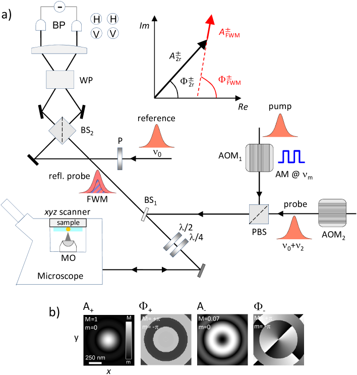
Figure 1: Four-wave mixing interferometry epi-detected dual-polarisation resolved. a) Sketch. Pump pulses are amplitude-modulated (AM) at $\nu_{\rm m}$ and probe pulses are frequency shifted by $\nu_{2}$, using acousto-optical modulators (AOMs). Pulses are coupled into an inverted microscope equipped with a high NA microscope objective (MO). Pump and probe beams are adjusted to be circularly polarized at the sample by $\lambda/4$ and $\lambda/2$ waveplates. Circular polarisations are transformed into horizontal (H) and vertical (V) linear polarisation by the same waveplates and both components are simultaneously detected through their interference with a frequency-unshifted reference linearly polarised at $45^{\circ}$. BP: Balanced photodiodes. WP: Wollaston prism deflecting beam out of drawing plane. (P)BS: (polarising) beam splitter. P: Polariser. Inset: amplitude ($A$) and phase ($\Phi$) of the reflected probe and FWM field, measured by a multi-channel lock-in, where +(-) refers to the co(cross) polarised component relative to the incident circularly polarized probe. b) Calculated field distribution in the focal plane of a 1.45 NA objective for an incident field left circularly polarized. $A_{+}$ $(A_{-})$ is the co (cross) polarised amplitude , and $\Phi_{+}$ ($\Phi_{-}$) the corresponding phase.

A sketch of the FWM technique is shown in Fig. 1a. The key developments in this new design compared to previous works are the epi-collection (reflection) geometry and the dual-polarisation heterodyne detection scheme. We use a train of femtosecond optical pulses with repetition rate $\nu_{\rm L}$ which is split into three beams, all having the same center wavelength, resulting in a triply degenerate FWM scheme. One beam acts as pump and excites the NP at the LSPR with an intensity which is temporally modulated with close to unity contrast by an acousto-optic modulator (AOM₁) driven at carrier frequency $\nu_{1}$ with a square wave amplitude modulation of frequency $\nu_{\rm m}$. The change in the NP optical properties induced by this excitation is resonantly probed by a second pulse at an adjustable delay time $\tau$ after the pump pulse. Pump and probe pulses of fields ${\mathbf{E}}_{1}$ and ${\mathbf{E}}_{2}$, respectively, are recombined into the same spatial mode and focused onto the sample by a high NA microscope objective. The sample can be positioned and moved with respect to the focal volume of the objective by scanning an $xyz$ sample stage with nanometric position accuracy. A FWM field ${\mathbf{E}}_{\rm FWM}$ (proportional to ${\mathbf{E}}_{1}{\mathbf{E}}_{1}^{*}{\mathbf{E}}_{2}$) is collected together with the probe in reflection (epi-direction) by the same objective, transmitted by the beam splitter (BS₁) used to couple the incident beams onto the microscope, and recombined in a second beam splitter (BS₂) with a reference pulse field (${\mathbf{E}}_{\rm R}$) of adjustable delay. The resulting interference is detected by two pairs of balanced photodiodes. A heterodyne scheme discriminates the FWM field from pump and probe pulses and detects amplitude and phase of the field. In this scheme, the probe optical frequency is slightly upshifted via a second AOM (AOM₂), driven with a constant amplitude at a radiofrequency of $\nu_{2}$, and the interference of the FWM with the unshifted reference field is detected. As a result of the amplitude modulation of the pump at $\nu_{\rm m}$ and the frequency shift of the probe at $\nu_{2}$, this interference gives rise to a beat note at $\nu_{2}$ with two sidebands at $\nu_{2}\pm\nu_{\rm m}$, and replica separated by the repetition rate $\nu_{\rm L}$ of the pulse train. A multi-channel lock-in amplifier enables the simultaneous detection of the carrier at $\nu_{2}-\nu_{\rm L}$ and the sidebands at $\nu_{2}\pm\nu_{\rm m}-\nu_{\rm L}$. Via the in-phase ($Re$) and in-quadrature ($Im$) components for each detected frequency, amplitude and phase of the probe field reflected by the sample $({\mathbf{E}}_{\rm 2r})$ and of the epi-detected FWM field are measured (see sketch in Fig. 1a).

A key point of the technique is the use of a dual-polarisation balanced detection. Firstly, probe and pump beams, linearly polarised horizontally (H) and vertically (V) respectively in the laboratory system, are transformed into cross-circularly polarized beams at the sample by a combination of $\lambda/4$ and $\lambda/2$ waveplates. The reflected probe and FWM fields collected by the same microscope objective travel backwards through the same waveplates, such that the probe reflected by a planar surface returns V polarized in the laboratory system. The reference beam is polarised at 45 degree (using a polariser) prior recombining with the epi-detected signal via the non-polarizing beamsplitter BS₂. A Wollaston prism vertically separates H and V polarizations for each arm of the interferometer after BS₂. Two pairs of balanced photodiodes then provide polarization resolved detection, the bottom (top) pair detecting the current difference (for common-mode noise rejection) of the V (H) polarised interferometer arms. In turn, this corresponds to detecting the co- and cross-circularly polarised components of ${\mathbf{E}}_{\rm 2r}$ and ${\mathbf{E}}_{\rm FWM}$ relative to the incident circularly polarized probe, having amplitudes (phases) indicated as $A_{\rm 2r}^{\pm}$ and $A_{\rm FWM}^{\pm}$ ($\Phi_{\rm 2r}^{\pm}$ and $\Phi_{\rm FWM}^{\pm}$) in the sketch in Fig. 1a where $+$ ($-$) refers to the co (cross) polarised component.

II The concept of nanometric localisation using optical vortices

To elucidate conceptually how the nanometric position accuracy arises from this dual-polarisation resolved FWM interferometry detection scheme, we simulated numerically the field distribution in the focal region of a 1.45 NA objective. The simulation parameters (wavelength, coverslip thickness, medium refractive index, back objective filling factor) were chosen to match the actual experimental conditions (see Methods). The amplitude and phase components of the field in the focal plane are shown in Fig. 1b for a left circularly ($\sigma^{+}$) polarised input field. Due to the high NA of the objective and the vectorial nature of the field, there is a significant cross-circularly polarised component that forms an optical vortex of topological charge $l=2$, i.e. it has an amplitude ($A_{-}$) which is zero in the focus center and radially-symmetric non-zero away from the center, and a phase ($\Phi_{-}$) changing with twice the in-plane polar angle. A point-like gold NP displaced from the focus center experiences this field distribution, and will in turn emit a field with an amplitude and a phase directly related to the NP radial and angular position. While this is the case for both reflected and FWM fields, only the FWM signal is background-free hence suited for tracking the NP in heterogeneous environments. In the following, we discuss the FWM field emitted from such NP and the corresponding coordinate retrieval.

We calculate the FWM field starting from the polarization of the NP at position $\mathbf{r}$ induced by the probe field, described by $\mathbf{p}(\mathbf{r})=\epsilon_{0}\epsilon_{\rm m}\hat{\alpha}\mathbf{E}_{2}(\mathbf{r})$ where $\epsilon_{0}$ is the vacuum permittivity, $\epsilon_{\rm m}$ is the dielectric constant of the medium surrounding the NP (glass and silicon oil in the experiment) and $\hat{\alpha}$ is the particle polarizability tensor. We calculate $\hat{\alpha}$ in the dipole approximation, valid for particle sizes much smaller than the wavelength of light (Rayleigh regime). To take into account non-sphericity of real particles, which will be relevant in the experiments as shown later, we adopted the model of a metallic ellipsoid with three orthogonal semi-axes of symmetry $a$, $b$ and $c$. In the particle reference system, $\hat{\alpha}$ is diagonal and its eigenvalues are given by bohren1998absorption $\alpha_{i}=4\pi abc(\epsilon-\epsilon_{\rm m})/(3\epsilon_{\rm m}+3L_{i}(\epsilon-\epsilon_{\rm m}))$, where $\epsilon$ is the dielectric permittivity of the particle, and $L_{i}$ with $i=a,b,c$ are dimensionless quantities defined by the particle geometry (see Supplementary Information section S1.i). For an arbitrary particle orientation in the laboratory system, the polarizability tensor can be transformed using $\hat{\alpha}=\hat{M}^{-1}\hat{\alpha}^{\prime}\hat{M}$ where $\hat{M}$ is a rotation matrix.

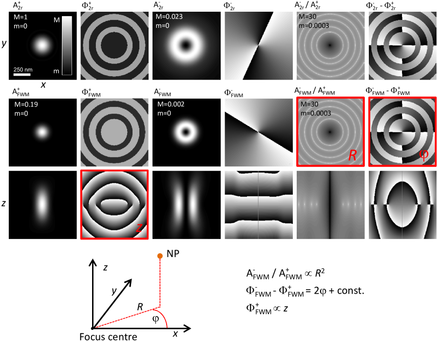
Figure 2: Nanometric localisation using optical vortices. Calculated amplitude (phase) components of the reflected probe field and FWM field $A_{\rm 2r}^{\pm}$ and $A_{\rm FWM}^{\pm}$ ($\Phi_{\rm 2r}^{\pm}$ and $\Phi_{\rm FWM}^{\pm}$) respectively, as a function of particle position in the sample focal plane $(x,y)$, and in a section along the axial direction $(x,z)$ through the focus, where + refers to the co-polarised component and - to the cross-polarised component relative to the left-circularly polarised incident probe. The calculation assumes a perfectly spherical gold NP in the dipole approximation. The inset shows a sketch of how the amplitude and phase of the FWM field ratio and the phase of the co-polarised FWM field can be used to locate in 3D the spatial position of the NP relative to the focus center. Linear grey scale from $-\pi$ to $\pi$ for all phases, and from m to M for field amplitudes, as indicated. The amplitude ratio of reflected probe and FWM are shown on a logarithmic greyscale over 5 orders of magnitudes.

The interference of the reflected probe field with the reference field is calculated using $E_{\rm 2r}^{\pm}=(\mathbf{E}_{\rm R}^{\pm})^{*}\cdot\hat{\alpha}\,{\mathbf{E}_{2}^{+}}$ where $\hat{\alpha}\,{\mathbf{E}_{2}^{+}}$ is the particle induced polarisation for a $\sigma^{+}$ polarised incident probe field (we dropped the constant $\epsilon_{0}\epsilon_{\rm m}$ in $\mathbf{p}$ for brevity), and $\mathbf{E}_{\rm R}^{\pm}$ are reference fields equal to left (+) and right (-) circularly polarised input fields. The technique is configured such that the optical mode of probe and reference fields are matched, hence $\mathbf{E}_{\rm R}$ was calculated as the field distribution in the focal region in the same way as $\textbf{E}_{2}$ (see Methods), and back-propagated via time reversal. Similarly, the FWM interference is calculated as $E_{\rm FWM}^{\pm}=(\mathbf{E}_{\rm R}^{\pm})^{*}\cdot\delta\hat{\alpha}\,{\mathbf{E}_{2}^{+}}$. Here, $\delta\hat{\alpha}$ is the pump-induced change of the particle polarizability which we have modeled as described in our previous work MasiaPRB12 . Briefly, $\delta\hat{\alpha}$ arises from the transient change of the electron and lattice temperature following the absorption of the pump pulse by the NP. $\delta\hat{\alpha}$ depends on the pump fluence at the NP, on the particle absorption cross-section, and on the delay time between pump and probe pulses (see also Supplementary Information Fig. S2 and S10). The simulations in Fig. 2 were performed to reproduce the experimentally measured FWM signal strength on a 30 nm radius gold NP at $\tau=0.5$ ps shown later (note that $\tau\sim 0.5$ ps is the delay for which the FWM amplitude reaches its maximum as a result of the ultrafast heating of the electron gas MasiaPRB12 ).

$E_{\rm 2r}^{\pm}$ and $E_{\rm FWM}^{\pm}$ have amplitudes and phases as a function of particle position in the focal region as shown in Fig. 2 for the case of a perfectly spherical NP. Similar to the spatial distributions of the focussed field shown in Fig. 1b, $E_{\rm 2r}^{-}$ and $E_{\rm FWM}^{-}$ form optical vortices of $l=2$ topological charge. The ratio $E_{\rm 2r}^{-}/E_{\rm 2r}^{+}$ is also shown with its amplitude $A_{\rm 2r}^{-}/{A_{\rm 2r}^{+}}$ and phase $\Phi_{\rm 2r}^{-}-\Phi_{\rm 2r}^{+}$. The FWM field distribution has a narrower PSF than the reflection, as expected from the third-order nonlinearity. The phase of $E_{\rm FWM}$ is shifted compared to $E_{\rm 2r}$ due to the phase difference between $\delta\hat{\alpha}$ and $\hat{\alpha}$. Slices along the axial direction ($z$) are shown for $E_{\rm FWM}$ (a similar behavior is observed for $E_{\rm 2r}$, see Supplementary Information Fig. S1). Of specific importance for the localization of the NP in 3D are the amplitude and phase of the FWM field ratio $E_{\rm FWM}^{-}/E_{\rm FWM}^{+}$ and the phase of the co-polarized $E_{\rm FWM}^{+}$ as highlighted by the red panels and sketch in Fig. 2.

The co-polarized FWM amplitude is much stronger ($\sim 90$ fold) than the cross-polarized FWM, and has a phase which is independent of the lateral position over the PSF width. Conversely, along the $z$-axis this phase is linear in the displacement between particle and center of the focus and can be used to determine the particle $z$ coordinate. This can be easily understood as due to the optical path length difference between the particle and the observation point. For a plane wave of wavevector $k=2{\pi}n/\lambda$ with $n$ refractive index in the medium the phase would be $2kz$, the factor of 2 accounting for the back and forth path in reflection geometry reflection. We find a linear relationship between $\Phi_{\rm FWM}^{+}$ and $z$ (see Supplementary Information Fig. S3) with a slope $\partial z/\partial\Phi=38.8$ nm/rad, slightly larger than $\lambda/(4\pi n)=28.8$ nm/rad. This is due to the propagation of a focussed beam with high NA where a Gouy phase shift occurs, reducing the wavevector in axial direction due to the wavevector spread in lateral direction.

For the in-plane radial coordinate $R$ of the NP position relative to the focus position (see sketch in Fig. 2), we find that the FWM amplitude ratio $A_{\rm FWM}^{-}/A_{\rm FWM}^{+}$ scales quadratically with $R$ up to $R\sim 60$ nm, such that this coordinate can be calculated as $R=R_{0}\sqrt{A_{\rm FWM}^{-}/A_{\rm FWM}^{+}}$. Notably, by using the FWM ratio the retrieved $R$ is independent of the pump, probe and reference powers, and of the NP size (in the dipole approximation). Conversely, $R_{0}$ is specific to the NA of the microscope objective used and the probe beam fill factor (see Supplementary Information Fig. S4) and decreases with increasing NA, showing that high NAs are required to localize the NP in $R$ down to small distances. Finally, the angular position coordinate $\varphi$ can be taken from the phase of the FWM ratio $\Theta=\Phi_{\rm FWM}^{-}-\Phi_{\rm FWM}^{+}$ as $\varphi=(\Theta-\Theta_{0})/2$ (see also Supplementary Information Fig. S3).

In essence, using these relationships we can locate the NP in 3D ($z$, $R$ and $\varphi$) by scanless polarisation-resolved and phase-resolved FWM acquisition at a single spatial point.

III Background-free Four-wave Mixing Detection

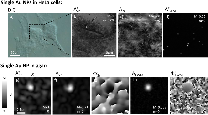
Figure 3: Background-free FWM detection of single NPs in heterogeneous environments. Top: Fixed HeLa cells that have internalized gold NPs of 20 nm radius imaged by (a) differential interference contrast (DIC) microscopy, (b) co-circularly polarised reflection amplitude $A_{\rm 2r}^{+}$, (c) cross-circularly polarised reflection amplitude $A_{\rm 2r}^{-}$, (d) co-circularly polarised FWM amplitude $A_{\rm FWM}^{+}$. FWM was acquired with pump-probe delay time of 0.5 ps, pump (probe) power at the sample of 30 $\mu$W (15 $\mu$W), 2 ms pixel dwell time, pixel size in plane of 95 nm and z-stacks over 6 $\mu$m in 250 nm z-steps. FWM is shown as a maximum intensity projection over the z-stack, while the reflection is on a single $(x,y)$ plane (scanning the sample position). Bottom: Single $(x,y)$ plane image of a 25 nm radius gold NP in 5% agarose gel, via the co-circularly polarised reflection amplitude $A_{\rm 2r}^{+}$ (e), cross-circularly polarised reflection amplitude $A_{\rm 2r}^{-}$ (f) and phase $\Phi_{\rm 2r}^{-}$ (g), co-circularly polarised FWM amplitude $A_{\rm FWM}^{+}$ (h) and phase $\Phi_{\rm FWM}^{+}$ (i). FWM was acquired with 0.5 ms pixel dwell time, pixel size in plane of 38 nm. Grey scales are linear from $-\pi$ to $\pi$ for all phases, and from m to M for field amplitudes, as indicated.

Prior to quantifying experimentally the nanometric localisation accuracy, it is important to emphasize that our FWM detection is background-free even in scattering and/or autofluorescing environments, making it applicable to imaging single small NPs inside cells, surpassing other methods reported in the literature. Localizing single plasmonic NPs with nanometric accuracy even at sub-millisecond exposure times can be achieved in an optically clear environment with simpler techniques such as dark-field microscopy UenoBJ10 and interferometric scattering microscopy Ortega-ArroyoPCCP12 . However, since these techniques use the linear response of the NP they are substantially affected by endogenous scattering and fluorescence, which severely limit their practical applicability in heterogeneous biological environments.

To exemplify this point, Fig. 3(top) shows fixed HeLa cells that have internalized gold NPs of 20 nm radius, imaged with FWM using a 1.45 NA oil-immersion objective. High-resolution DIC microscopy was available in the same instrument (for details see Supplementary Information section S2.iii and S2.vii). Fig. 3a shows the DIC image of a group of HeLa cells on which reflection and FWM imaging was performed in the region highlighted by the dashed frame. The co-circularly polarized reflection image $A_{\rm 2r}^{+}$ shown in Fig. 3b correlates with the cell contour seen in DIC, and shows a spatially varying contrast due to thickness and refractive index inhomogeneities in the sample. Even with a particle diameter as large as 40 nm, gold NPs are not distinguished from the cellular contrast neither in DIC nor in the $A_{\rm 2r}^{+}$ reflection image. Detecting the cross-polarized reflection $A_{\rm 2r}^{-}$ (Fig. 3c) which has been suggested as a way to improve contrast MilesACSPhotonics15 is still severely affected by the cellular scattering background. On the contrary, the co-circularly polarised FWM amplitude $A_{\rm FWM}^{+}$ shown in Fig. 3d as maximum intensity projection over a 6 ${\mu}$m $z$-stack is background-free (throughout the $z$-stack) and clearly indicates the location of single gold NPs in the cell. Notably, FWM acquisition can be performed simultaneously with confocal fluorescence microscopy for correlative co-localisation analysis, as shown in the Supplementary Information Fig. S11.

Fig. 3(bottom) shows a single 25 nm radius gold NP embedded in a dense (5% w/v) agarose gel. The scattering from the gel is visible as a structured background in the co-circularly polarized reflection image $A_{\rm 2r}^{+}$ in Fig. 3e. Detecting the cross-polarized reflection (Fig. 3f) again does not eliminate the background. With the reflection amplitude scaling as the volume of the particle, a 15 nm radius NP would be indistinguishable from the background in the present case. Furthermore, the interference with the background limits the accuracy of particle localization. Notably, the phase $\Phi_{\rm 2r}^{-}$ is also severely affected by the scattering from the gel. Conversely, the FWM amplitude $A_{\rm FWM}^{+}$ and phase $\Phi_{\rm FWM}^{+}$ shown in Fig. 3h,i are background-free (as can be seen by the random phase outside the particle) and clearly resolve the NP despite the heterogeneous surrounding.

IV Experimental localisation: The role of nanoparticle ellipticity

To experimentally quantify the nanometric localisation and its accuracy due to photon shot-noise, we started by examining a single nominally spherical 30 nm radius gold NP drop cast onto a glass coverslip and immersed in silicon oil, using an index-matched 1.45 NA oil-immersion objective.

The experimental data shown in Fig. 4 are scans of the $(x,y,z)$ sample position. They reveal all main features seen in the calculations, namely a ring-like spatial distribution in-plane of the amplitude ratio $A_{\rm FWM}^{-}/A_{\rm FWM}^{+}$ and a phase of the cross-polarized component, and in turn of the FWM ratio, twice rotating from 0 to $2\pi$ along the in-plane polar angle. A main difference to the calculations is the observation of two displaced nodes, rather than a single central node, in the amplitude of the cross-polarized component, and in turn a nearly constant phase of the cross-polarized component in the central area. The FWM ratio resolved across different axial planes is also shown in Fig. 4. We observe that, besides these minima, the axially resolved distributions agree with the calculated behavior of a linear relationship between $\Phi_{\rm FWM}^{+}$ and $z$ and a $z$-dependent $\Theta_{0}$ manifesting as a rotated phase pattern of $\Theta=\Phi_{\rm FWM}^{-}-\Phi_{\rm FWM}^{+}$ for different $z$-planes.

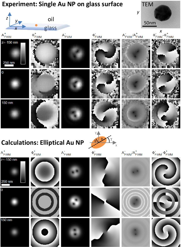
Figure 4: FWM of a single NP attached on glass. Amplitude and phase as a function of NP position in the $(x,y)$ plane at different axial positions $z$. Linear grey scale from $-\pi$ to $\pi$ for phases, and from $m$ to $M$ for field amplitudes. The amplitude ratio is on a logarithmic scale over 4 orders of magnitudes. Experiment: Top inset shows a sketch of the sample and a TEM image of a typical NP from the batch used. Pump (probe) power at the sample was 18 $\mu$W (9 $\mu$W), 3 ms pixel dwell time, 0.5 ps pump-probe delay time, pixel size in-plane (axial) was 17 nm (75 nm). Calculations assume particle asphericity in plane with semi-axes $a=30.135$ nm and $b=30$ nm (see text).

Notably, by measuring on $>50$ particles in the sample we could not find any pattern forming a $l=2$ optical vortex as simulated in Fig. 2. Different particles showed minima with different relative displacement, or single displaced minima, or no minima within the spatial range of sufficient signal to noise (see Supplementary Information Fig. S12), suggesting that these minima are related to physical differences between particles. Indeed, we can explain these experimental findings assuming a small particle asphericity. This is shown in the calculations in Fig. 4 where we used an ellipsoid nanoparticle with semi-axes $a=30.135$ nm and $b=c=30$ nm along the $x$, $y$ and $z$ axis in the particle reference system, which is rotated in plane relative to the laboratory system (see also see Supplementary Information Fig. S5 and S6). It is remarkable that an asymmetry of only 0.5% in aspect ratio, or about one atomic layer of gold, manifests as a significant perturbation of the cross-polarized field patterns compared to the spherical case. With such sensitivity to asymmetry, the lack of experimentally observed pattern corresponding to a perfectly spherical particle is not surprising, considering the real particle morphology as observed in transmission electron microscopy (TEM) for this sample (see top inset in Fig. 4 and Supplementary Information Fig. S8).

The shot-noise in the experiment as well as the deviation from perfect sphericity affect the localisation accuracy. This is analyzed in Fig. 5. Firstly, we performed simulations as in Fig. 2 for a perfectly spherical particle including experimental shot-noise. The experimental shot-noise was evaluated by taking the statistical distribution of the measured FWM field (in both the in-phase $Re$ and in-quadrature $Im$ components) in a spatial region away from the particle, where no FWM is detectable. The standard deviation $\sigma$ of this distribution was deduced, and was found to be identical in both components, and for the co-polarised and cross-polarised components, as expected for an experimental noise dominated by the shot-noise in the reference beam (see Supplementary Information Fig. S9 for the dependence of $\sigma$ on the power in the reference beam). A relative noise figure was defined as $\sigma/A_{0}$ with $A_{0}$ being the maximum measured value of the co-polarized FWM field amplitude. The simulations were performed using a statistical distribution of the FWM field values ($Re$ and $Im$ components) at each spatial pixel having the same relative noise $\sigma/A_{0}$ as the experimental data.

To quantify the uncertainty in the localisation of the particle coordinates, we then calculated the deviation $\Delta=\sqrt{(x-x_{\rm s})^{2}+(y-y_{\rm s})^{2}+(z-z_{\rm s})^{2}}$ between the set position of the NP in 3D ($x_{\rm s},y_{\rm s},z_{\rm s}$) and the deduced position ($x,y,z$) using the FWM field amplitude and phase as detailed above. The resulting $\Delta$ in the focal plane $(x,y,0)$ and in the $(x,0,z)$ cross-section along the axial direction are shown in Fig. 5a for the ideal case as in Fig.2, and in Fig. 5b when adding a relative noise of 0.07% corresponding to the experiment in Fig. 4. $\Delta\neq 0$ in the ideal case is a measure of the validity of the assumed dependencies, in particular the quadratic behavior in the radial coordinate $R$, which becomes inaccurate for $R>60$ nm as discussed. This deviation can be easily removed by including a $R^{4}$ term (see Supplementary Information Fig. S3). Notably, in the region where the assumed trends are valid, we observe that adding the experimental noise results in a localization uncertainty of less than 20 nm. Increasing the relative noise by one order of magnitude to 0.7% results in a localization uncertainty of $\sim 50$ nm, as shown in Fig. 5c. We emphasize that $\Delta$ is dominated by the in-plane uncertainty, i.e. $\Delta=\sqrt{(x-x_{\rm s})^{2}+(y-y_{\rm s})^{2}+(z-z_{\rm s})^{2}}\cong\sqrt{(x-x_{\rm s})^{2}+(y-y_{\rm s})^{2}}$. In fact, considering that the axial direction $z$ is determined directly by the slope of $\Phi_{\rm FWM}^{+}$ and does not involve the cross-polarized FWM, we find $z$ localization accuracies as small as 0.3 nm for 0.7% noise in $\Phi_{\rm FWM}^{+}$.

Note that the relative shot-noise in the experiments scales as $1/\left(V\sqrt{t}{I_{1}}\sqrt{I_{2}}\right)$ where $V$ is the particle volume (in the Rayleigh regime), $I_{1}$ ($I_{2}$) is the intensity of the pump (probe) beam at the sample, and $t$ is the acquisition time. It can therefore be adjusted according to the requirements. For example, a 15 nm radius NP imaged under the experimental conditions as in Fig. 4 would give rise to an 8-fold increase in relative noise, hence still maintaining the localization uncertainty to below 50 nm. These results elucidate that a localization accuracy of below 20 nm in-plane and below 1 nm in axial direction is achievable with the proposed method with a realistic shot-noise level as in the experiment.

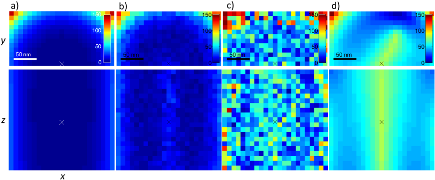
Figure 5: Position localisation accuracy. Difference between the set position of the nanoparticle in 3D and the deduced position using the FWM field amplitude and phase with the coordinate reconstruction parameters as described in the text. The color bar gives the values of this difference in nanometer. Top panels show maps in the $(x,y)$ plane, bottom panels are axial $(x,z)$ maps. The cross shows the position of the focus center. a) Spherical particle without shot-noise; b) Spherical particle with relative shot-noise of 0.07% as in the experiment in Fig. 4; c) spherical particle with relative shot-noise of 0.7%; d) asymmetric particle with semi-axis $a=30.135$ nm and $b=c=30$ nm, as in the simulations in Fig. 4.

However, the lack of particle symmetry is a limitation for the in-plane localization. Introducing the particle asymmetry, without shot-noise, as calculated in Fig. 4, results in a significant deviation $\Delta\sim 100$ nm in the central area, due to the lack of a central node in the cross-polarized FWM amplitude (see Fig. 5d). On the other hand, it is remarkable how sensitive the described FWM technique is to particle asymmetry, which can be used as a new tool to detect particle ellipticity down to $a/b-1=10^{-4}$ (corresponding to atomic accuracy comparable to TEM) as well as particle orientation. We find that the FWM amplitude ratio in the focus center scales linearly with the particle ellipticity and that the phase of the FWM ratio in the focus center scales with the in-plane particle orientation angle (which for the data in Fig.4 was found to be $\gamma=150^{\circ}$, see Supplementary Information Fig. S5 and S6).

The limitation of particle asymmetry can be overcome by improving colloidal fabrication techniques. For example, it has been reported in the literature that gold nanorods can be synthesized as single crystals without stacking faults or dislocations KatzBonnNL11 , and can be shaped to become spherical particles under high-power femtosecond laser irradiation TaylorACSNano14 . We also note that when examining gold NPs of 5 nm radius (see Supplementary Information Fig. S8 and S13), we found a large proportion ($\sim 70\%$) having a FWM amplitude ratio $A_{\rm FWM}^{-}/A_{\rm FWM}^{+}\leq 0.02$ in the center of the focal plane, in this case limited by the signal-to-noise ratio rather than the particle asymmetry, suggesting that smaller NPs might be intrinsically more mono-crystalline hence symmetric.

Importantly, when NPs are not immobilized onto a surface but freely rotating (a more relevant scenario for particle tracking applications) we can expect that the rotational averaging over the acquisition time (the rotational diffusion constant in water at room temperature of a 30 nm radius nanoparticle is $\sim 10^{4}$ rad²/s) would result in an effective symmetry, and would lead to a localization accuracy only limited by shot-noise. This case is discussed in the next section.

V Rotational averaging

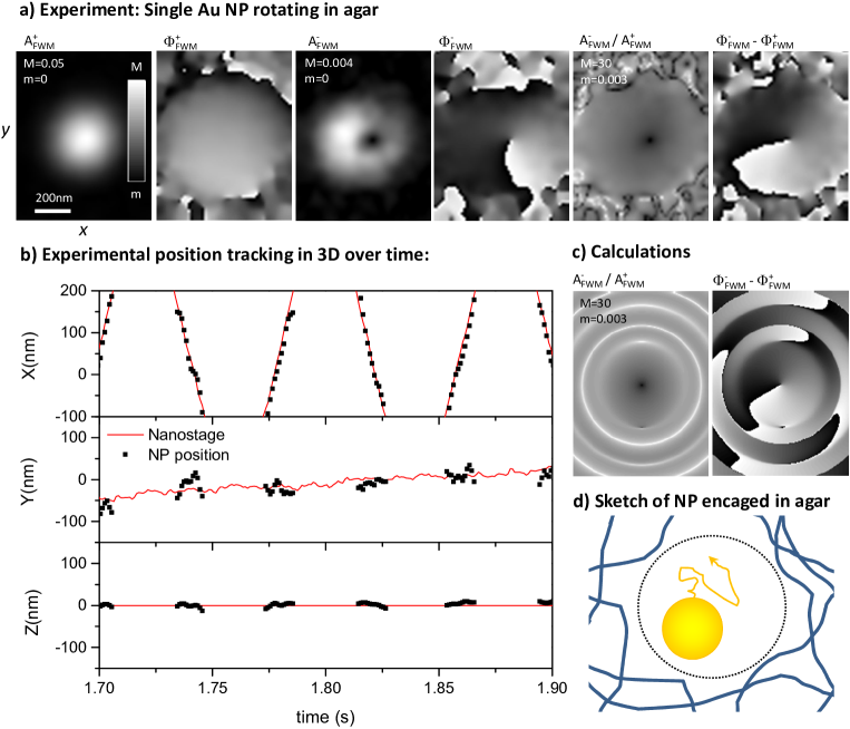
Figure 6: Rotational averaging of nanoparticle asymmetry. Single 25 nm radius gold NP freely rotating while encaged in an agarose gel pocket (see sketch). a) Experimental $xy$ scan of the cross and co-circularly polarised FWM field in the focal plane, using a 1.27 NA water-immersion objective. Linear grey scale from $-\pi$ to $\pi$ for phases, and from $m$ to $M$ for field amplitudes with $M$ given relative to the maximum $A_{\rm 2r}^{+}$. The amplitude ratio is on a logarithmic scale over 4 orders of magnitudes. Pump (probe) power at the sample was 70 ${\mu}$W (10 ${\mu}$W) with pump (probe) filling factor 2.15 (0.97). Measurements were performed with 0.5 ms pixel dwell time, 0.5 ps pump-probe delay time, and 13 nm pixel size in-plane. Data are shown as spatial averages over an effective area of $3\times 3$ pixels. b) Time traces of the retrieved particle position coordinates in 3D from the measured FWM amplitude and phase (symbols) compared with the coordinates recorded from the scanning piezoelectric sample stage (lines). Traces are binned to an equivalent 1 ms acquisition time. c) Calculated FWM field ratio assuming a polarisation tensor that projects the longitudinally polarised field component into the $(x,y)$ plane (see text).

To mimic a relevant biological environment such as the cytosolic network, as well as having single NPs freely rotating but not diffusing out of focus, gold NPs of 25 nm radius were embedded in a dense (5% w/v) agarose gel in water (see Supplementary Information section S2.ii) and measured using an index-matched 1.27 NA water-immersion objective. For these experiments the focused size of the pump beam was increased by a factor of two (by under-filling the back focal aperture), to enlarge the region where a single NP could diffuse while still being excited by the pump field hence giving rise to FWM (this also increases the maximum cross-polarized FWM amplitude). Conversely, the probe beam was tightly focused to exploit the full NA of the objective an in turn exhibit an $l=2$ optical vortex in the cross-circularly polarised component as calculated in Fig. 2.

Fig. 6a shows an $xy$ scan of the measured cross and co-circularly polarised FWM field in the focal plane, and the corresponding ratio in amplitude and phase, on a single NP while freely rotating but being enclosed in a tight pocket of the agar network resulting in a negligible average translation during the measurement time (for an estimate of the size of the pocket see Supplementary Information section S2.xi). As expected, the rotational averaging enables the observation of an optical vortex with a central amplitude node in the cross-circulalry polarised FWM. Surprisingly however, the phase pattern reveals an $l=1$ vortex, as opposed to the predicted $l=2$, i.e. the phase is directly changing with the in-plane polar angle instead of twice. Calculations show that for an incident circularly polarised field, the longitudinally polarised component ($E_{\rm z}$) in the focus of a high NA objective has this symmetry, and we can reproduce the experimental findings by introducing a particle polarisability tensor which projects the longitudinal component into the $xy$ plane (see Supplementary Information Section S1.vii). Conversely, it is not possible to reproduce the experimental findings by assuming a non-rotating randomly-oriented asymmetric particle (see Supplementary Information Section S2.xii), hence free rotation is key to the pattern observed in Fig. 6a. Since the only particle asymmetry that does not average upon rotation is 3D chirality, we suggest that this response is a manifestation of chirality (albeit a detailed theoretical understanding of the nonlinear optical response of a chiral particle is beyond the scope of this work). We remind that these quasi-spherical NPs have irregularities of few atoms clusters which can lead to symmetry breaking, as already seen for their ellipticity, and thus also 3D chirality (see TEM in Supplementary Information Fig. S8). Notably, an $l=1$ optical vortex offers a simpler dependence for the retrieval of the NP position coordinates, with a FWM amplitude ratio $A_{\rm FWM}^{-}/A_{\rm FWM}^{+}$ scaling linearly with $R$ and a phase $\Theta=\Phi_{\rm FWM}^{-}-\Phi_{\rm FWM}^{+}$ directly changing with the polar angle $\varphi$ (see Supplementary Information Fig. S14). Using these dependencies (alongside the axial position $z$ given by $\Phi_{\rm FWM}^{+}$ as previously shown), we have retrieved the NP position coordinates in 3D for the scan shown in Fig. 6a and compared them with the position coordinates recorded from the scanning piezoelectric sample stage. This is shown in Fig. 6b. We observe deviations below 50 nm in $x,y$ between the retrieved NP positions and the coordinates from the stage and a remarkable accuracy in $z$ better than 10 nm, limited by systematic drifts rather than shot-noise. From the shot noise $\sigma/A_{0}=0.007$ in these measurements and the coordinate retrieval parameters, we deduce the uncertainty to be below 20 nm in $x,y$ and 1 nm in $z$, using only 1 ms acquisition time.

VI Single particle tracking

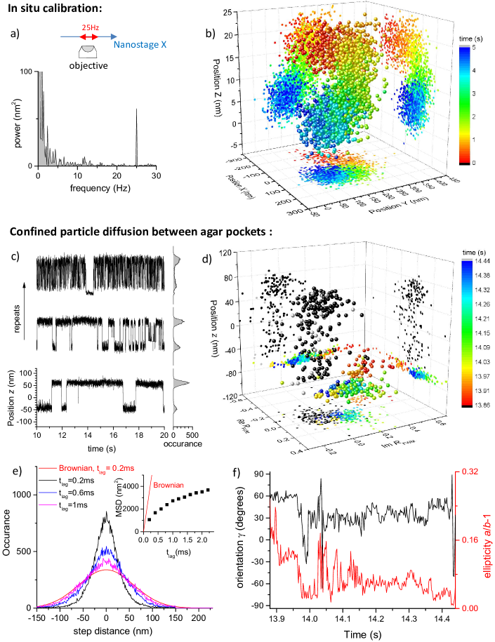
Figure 7: In situ calibration and nanoparticle tracking. a) Power spectrum of FWM field ratio showing the 25 Hz oscillation imposed onto the sample stage for calibration, as sketched. b) Retrieved position coordinates versus time of a single 25 nm radius NP in agar (2 ms per point). c) Axial position time traces of a single gold NP while jumping between two gel pockets. d) Zoom of top trace in (c) showing the axial position and FWM field ratio dominated by the NP asymmetry; corresponding in-plane ellipticity and orientation are in f). e) Analysis of axial position time traces acquired at 0.2 ms per point (see text).

A demonstration of the practical applicability of the method for scanless single particle tracking in 3D is shown in Fig. 7 on gold NPs of 25 nm radius embedded in a dense (5% w/v) agarose gel in water, which provides a heterogeneous environment as shown in Fig. 3(bottom). For practical purposes, we implemented a simple in situ calibration of the in-plane NP position coordinates without the need for prior knowledge and/or characterization of the particle optical response. As shown in Fig. 7a, we apply a small oscillation of known amplitude (16 nm) and frequency (25 Hz) to one axis of the sample stage. When the FWM field ratio from the NP encodes the NP in-plane position as discussed in the previous section, this oscillation is detected in the measured $E_{\rm FWM}^{-}/E_{\rm FWM}^{+}$ with an amplitude and a phase which we can use to directly calibrate the FWM field ratio in terms of in-plane position coordinates of known size and direction (see also Supplementary Information section S2 x.iii). Fig. 7a shows the power spectrum of the Fourier transform of $E_{\rm FWM}^{-}/E_{\rm FWM}^{+}$ which exhibits a peak at this modulation frequency. The correspondingly calibrated particle position coordinates over time are shown Fig. 7b. Conversely, if for a NP we do not observe this oscillation in $E_{\rm FWM}^{-}/E_{\rm FWM}^{+}$, the FWM field ratio is a measure of the NP in-plane asymmetry and orientation. This case is shown in Fig. 7c-d (for the power spectrum see Supplementary Information section S2 x.iii). Importantly, we can still accurately measure the axial position coordinate, which is directly given by $\Phi_{\rm FWM}^{+}$ and does not involve the cross-polarized FWM, while now $E_{\rm FWM}^{-}/E_{\rm FWM}^{+}$ encodes information on the NP asymmetry and orientation, rather than its in-plane position. Fig. 7c shows examples of traces of the NP $z$ position acquired over several tens of seconds (with 2 ms point acquisition) from which we can see a ’jumping behavior’ around two preferred axial locations, suggesting the presence of two pockets in the agar gel separated by about 100 nm. Fig. 7d shows the $z$ position together with $E_{\rm FWM}^{-}/E_{\rm FWM}^{+}$ (as real and imaginary parts) as a zoom over a time window (from the top trace in (c)) during which the NP got stuck in a corner, below the center of the lower pocket. From the strong and slowly varying FWM field ratio, the corresponding time evolution of the NP in-plane orientation angle and aspect ratio is given in Fig. 7f. Finally, Fig. 7e shows the analysis from an axial position time trace acquired at high speed (0.2 ms time per point, for over 10 s), indicating constrained diffusion. The traces were analyzed by calculating the mean square displacement (MSD) as a function of time lag ($t_{\rm lag}$) ManzoRPP15 . Histograms of the displacement for different $t_{\rm lag}$ are shown in Fig. 7e. The variance of the histogram gives the MSD, which is plotted versus $t_{\rm lag}$ in the inset. For Brownian diffusion MSD$=2Dt_{\rm lag}$ (for each dimension in space), with the free diffusion coefficient $D$ in water given in the Supplementary Information section S2 xi. The resulting linear behavior is shown as red line (and red Gaussian histogram) in Fig. 7e. The observed sub-linear dependence and saturation of MSD versus $t_{\rm lag}$ indicates confined diffusion.

VII Discussion and Conclusion

We have shown a new method to determine the position of a single non-fluorescing gold NP with nanometric accuracy in three dimensions from scanless far-field optical measurements. The method is based on the interferometric detection of the polarisation-resolved resonant FWM field in amplitude and phase, with a high numerical aperture objective. The displacement of the nanoparticle from the center focus in the axial direction is directly determined from the epi-detected FWM field phase, while the in-plane displacement manifests as a cross-circularly polarized component due to the optical vortex field pattern in the focus of a high numerical aperture objective, the amplitude and phase of which enables accurate position retrieval.

Shape asymmetry of the NP of as little as 0.5% ellipticity, corresponding to about one atomic layer of gold, also induces a cross-circularly polarized field. This exceptional sensitivity to asymmetry eventually limits accurate position retrieval in-plane. This can be overcome by observing a NP freely rotating, such that rotational averaging of the asymmetry occurs over the acquisition time.

Experimentally, we show that the FWM detection is completely background-free in scattering environments such as biological cells, and outperforms existing methods such as reflectometry, scattering and differential interference contrast. A localization accuracy of below 50 nm in-plane, and below 10 nm axial, limited by systematic drifts, is shown with a single NP of 25 nm radius freely rotating in an agarose gel, at an acquisition time of only 1 ms. The shot-noise limited accuracy is found to be below 20 nm in plane and 1 nm axially. Smaller NPs can be measured by correspondingly increasing the intensity of the incident beams and/or the acquisition time. Notably, we find that, during free rotation, the cross-circularly polarized FWM field distribution in the focal plane is an $l=1$ optical vortex, as opposed to the predicted $l=2$ for a perfectly spherical particle, and we suggest that this is a manifestation of NP chirality not averaged during rotation.

To demonstrate the practical applicability of the method for single particle tracking, we provide two examples of NPs diffusing in a dense agarose gel network. In one case, we show particle position coordinates retrieved using an in situ calibration procedure and the corresponding tracking in 3D. In the second case, we show that when the cross-circularly polarized component is dominated by the effect of shape asymmetry, it can be used for tracking the in-plane asymmetry and orientation, while the axial position coordinate provides information on the particle diffusion.

Ultimately, this method paves the way towards a new form of single particle tracking, where not only the NP position, but also its asymmetry, orientation, and chirality are detected with sub-millisecond time resolution, revealing much more information about the NP and its complex dynamics (e.g. hindered rotation) while moving and interacting within a disordered 3D environment.

VIII Appendix: Methods

FWM experimental set-up. Optical pulses of 150 fs duration centered at 550 nm wavelength with $\nu_{\rm L}=80$ MHz repetition rate were provided by the signal output of an optical parametric oscillator (Newport/Spectra Physics, OPO Inspire HF 100) pumped by a frequency-doubled femtosecond Ti:Sa laser (Newport/Spectra Physics, Mai Tai HP). In the experiment, the amplitude modulation frequency of the pump beam was $\nu_{\rm m}=0.4$ MHz. The MO was either a $100\times$ magnification oil-immersion objective of 1.45 NA (Nikon CFI Plan Apochromat lambda series) or a $60\times$ magnification water-immersion objective of 1.27 NA (Nikon CFI Plan Apochromat lambda series, super resolution) mounted into a commercial inverted microscope stand (Nikon Ti-U). The sample was positioned with respect to the focal volume of the objective by an $xyz$ piezoelectric stage with nanometric position accuracy (MadCityLabs NanoLP200). A prism compressor was used to pre-compensate the chirp introduced by all the optics in the beam path, to achieve Fourier limited pulses of 150 fs duration at the sample. Furthermore, since the reference beam does not travel through the microscope objective, glass blocks of known group velocity dispersion were added to the reference beam path, in order to match the chirp introduced by the microscope optics and thus maximize the interference between the reflected FWM field and the reference field at the detector. AOM₂ was driven at $\nu_{2}=$82 MHz. BS₁ is a 80:20 transmission:reflection splitter, transmitting most of the signal. We used balanced silicon photodiodes (Hamamatsu S5973-02) with home-built electronics and a high-frequency digital lock-in amplifier (Zürich Instruments HF2LI) providing six dual-phase demodulators, enabling to detect for both polarizations the carrier at $\nu_{2}-\nu_{\rm L}=2$ MHz and both sidebands at $\nu_{2}\pm\nu_{\rm m}-\nu_{\rm L}=2\pm 0.4$ MHz. This scheme overcomes the limitation in our previous work of using two separated lock-ins with associated relative phase offset MasiaPRB12 and provides an intrinsic phase referencing and a noise reduction via the detection of both side bands (see Supplementary Information section S2.iv).

Numerical simulations. The field in the focal area is calculated using PSF Lab - a software package that allows calculation of the point spread function of an aplanatic optical system Nasse2010 . For the calculations in Fig. 2 and Fig. 4 the simulation parameters - wavelength $\lambda$, objective lens NA, coverslip thickness $d$, medium refractive index $n$, back objective filling factor $\beta$ - were chosen to match the actual experimental conditions in Fig. 4, namely $\lambda=550$ nm, NA=1.45, $d=0.17$ mm, $n=1.5185$, and $\beta=0.83$. The filling factor is defined as $\beta=a/w$, where $a$ is the aperture radius of the objective lens and $w$ is the Gaussian parameter in the electric field radial dependence at the objective aperture $E=E_{0}e^{(-r^{2}/w^{2})}$. For the calculations in Fig. 6 the simulation parameters were NA=1.27, $n=1.333$, $\beta=2.15$ for the pump and $\beta=0.97$ for the probe beam. The calculation was performed for a linear polarization of the incident field along the $x$ axis. This results in a vectorial field at the focus called $\mathbf{E}^{x}(\mathbf{r})$. For the orthogonal linear incident polarization, the results were rotated counterclockwise to obtain $\mathbf{E}^{y}$. To simulate circular incident polarization, the calculated field maps $\mathbf{E}^{x}$ and $\mathbf{E}^{y}$ were combined with complex coefficients, namely: $\mathbf{E}^{+}=\frac{1}{\sqrt{2}}\left(\mathbf{E}^{x}+i\mathbf{E}^{y}\right)$, $\mathbf{E}^{-}=\frac{1}{\sqrt{2}}\left(\mathbf{E}^{x}-i\mathbf{E}^{y}\right)$ for left and right circular polarization, respectively.

IX Acknowledgments

This work was funded by the UK EPSRC Research Council (grant n. EP/I005072/1, EP/I016260/1, EP/L001470/1, EP/J021334/1 and EP/M028313/1) and by the EU (FP7 grant ITN-FINON 607842). P.B. acknowledges the Royal Society for her Wolfson Research Merit award (WM140077). We acknowledge Lukas Payne for help in sample preparation and TEM characterization and Peter Watson, Paul Moody and Arwyn Jones for help in cell culture protocols.

X Data availability

Information about the data created during this research, including how to access it, is available from Cardiff University data archive at http://doi.org/10.17035/d.2017.0031438581.

XI Author contributions

P.B. and W.L. conceived the technique and designed the experiments. W.L. wrote the acquisition software. F.M. performed preliminary experiments and calculations. G.Z. performed the final calculations, and the experiments on NPs attached onto glass. N.G. performed the experiments on cells and prepared NPs in agar. W.L. and P.B. performed the experiments on NPs in agar. P.B. wrote the manuscript. All authors discussed and interpreted the results and commented on the manuscript.

Background-free 3D nanometric localisation and sub-nm asymmetry detection of single plasmonic nanoparticles by four-wave mixing interferometry with optical vortices - Supplementary Information

S1 Calculations

i Polarisability of a non-spherical gold nanoparticle

We describe a non-spherical nanoparticle (NP) as a metallic ellipsoid with three orthogonal semi-axes of symmetry $a$, $b$ and $c$. In the particle reference system the polarisability tensor $\hat{\alpha}$ is diagonal, and its eigenvalues are given by bohren1998absorption

$$\alpha_{i}=4\pi abc\frac{\epsilon-\epsilon_{\rm m}}{3\epsilon_{\rm m}+3L_{i}(\epsilon-\epsilon_{\rm m})}\,,$$ (S1)

where $\epsilon$ is the dielectric constant of the NP, $\epsilon_{\rm m}$ is the dielectric constant of the surrounding medium, and $L_{i}$ with $i=a,b,c$ are dimensionless quantities defined by the NP geometry as

$$L_{a}=\frac{abc}{2}\int_{0}^{\infty}(a^{2}+q)^{-\frac{3}{2}}(b^{2}+q)^{-\frac{1}{2}}(c^{2}+q)^{-\frac{1}{2}}dq$$ (S2)

$$L_{b}=\frac{abc}{2}\int_{0}^{\infty}(a^{2}+q)^{-\frac{1}{2}}(b^{2}+q)^{-\frac{3}{2}}(c^{2}+q)^{-\frac{1}{2}}dq$$

$$L_{c}=\frac{abc}{2}\int_{0}^{\infty}(a^{2}+q)^{-\frac{1}{2}}(b^{2}+q)^{-\frac{1}{2}}(c^{2}+q)^{-\frac{3}{2}}dq$$

Only two out of three geometrical factors are independent, since for any ellipsoid $L_{a}+L_{b}+L_{c}=1$. For a spherical particle $a=b=c$, and

$$L_{1}=L_{2}=L_{3}=\frac{a^{3}}{2}\int_{0}^{\infty}(a^{2}+q)^{-5/2}dq=\frac{1}{3}$$ (S3)

For prolate spheroids (i.e. cigar-shaped) with $a>b=c$ or oblate (i.e. pancake-shaped) spheroids with $a=b>c$ the geometrical factors can be expressed analytically bohren1998absorption . In the most general case, we calculated the integrals in Eq. S2 using the numerical integration function integral of Matlab.

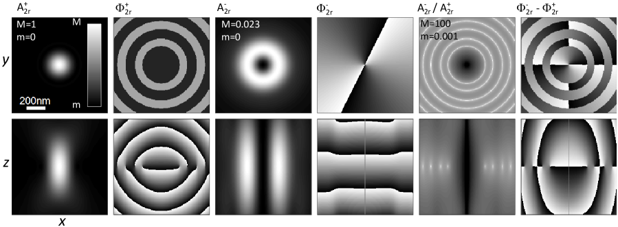
Figure S1: Calculated amplitude and phase of the reflected probe field $A_{\rm 2r}^{\pm}$ and $\Phi_{\rm 2r}^{\pm}$, as function of the NP position, in the $(x,y)$ focal plane, and in the $(x,z)$ plane through the focus. Here $+$ refers to the co-polarised component and $-$ to the cross-polarised component relative to the left-circularly polarised incident probe. The calculation assumes a perfectly spherical gold NP in the dipole approximation. Linear grey scale from $-\pi$ to $\pi$ for phases, and from $m$ to $M$ for field amplitudes, as indicated. The amplitude ratio is shown on a logarithmic scale over 5 orders of magnitude as indicated.

ii Reflected probe field

Fig. S1 shows the reflected probe field as function of the NP position, calculated as in Fig. 2 of the main manuscript, including its axial dependence through the focus.

iii Pump-induced change of particle polarisability: Spatial distribution

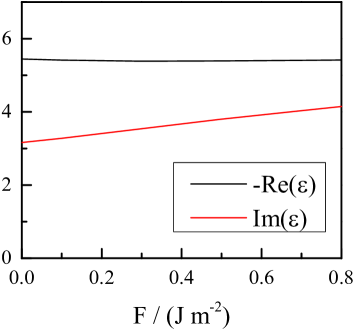
Figure S2: Calculated dependence of the real and imaginary part of the gold dielectric function $\epsilon$ assuming isotropic absorption by a 30 nm radius gold NP as a function of the pump fluence, for a pump and probe wavelength of 550 nm and a delay time of 0.5 ps. Other parameters as described in the methods section of the main text.

To calculate the pump-induced change of the particle polarizability $\delta\hat{\alpha}$ we used the model developed in our previous work MasiaPRB12 . Briefly, $\delta\hat{\alpha}$ arises from the transient change of the electron and lattice temperature following the absorption of the pump pulse by the nanoparticle, and therefore depends on the pump fluence at the NP, on the absorption cross-section of the NP, and on the delay time between pump and probe pulses. We calculated the change in the gold dielectric function $\epsilon$ as in Ref. MasiaPRB12, as a function of pump fluence at the particle, using the absorption cross-section of a 30 nm radius gold NP, for a pump-probe wavelength of 550 nm and delay time of 0.5 ps. The result is shown in Fig. S2. To account for the spatial profile of the pump we use the pump intensity spatial distribution $|\mathbf{E}_{1}^{-}(\mathbf{r})|^{2}$ to deduce $\epsilon(\mathbf{r})$ in the presence of the pump, and in turn $\delta\hat{\alpha}(\mathbf{r})$.

iv Parameters for NP position localisation

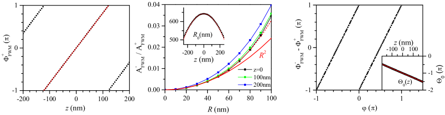
Figure S3: Left: Calculated axial dependence of the phase of the co-polarised FWM component (symbols) together with a linear fit (red line) having the slope $\partial z/\partial\Phi=38.8$ nm/rad. Middle: Radial dependence of the cross to co-polarised FWM amplitude ratio for three different axial positions as indicated. The red solid line shows a fit assuming the quadratic dependence $(R/R_{0})^{2}$ at the focal plane $z=0$, while the red dashed line assumes the dependence $(R/R_{0})^{2}+(R/R_{1})^{4}$. Inset: Dependence of $R_{0}$ on the axial position. Right: Phase of the cross to co-polarised FWM ratio $\Theta=\Phi_{\rm FWM}^{-}-\Phi_{\rm FWM}^{+}$ versus polar angle in the $z=0$ plane, following the relationship $\varphi=(\Theta-\Theta_{0})/2$. Inset: $\Theta_{0}$ versus axial position.

From the calculations in Fig. 2 of the main manuscript we find a linear relationship between $\Phi_{\rm FWM}^{+}$ and $z$ as shown in Fig. S3 with a slope $\partial z/\partial\Phi=38.8$ nm/rad, slightly larger than $\lambda/(4\pi n)=28.8$ nm/rad. This is due to the propagation of a focussed beam with high NA where a Gouy phase shift occurs, effectively increasing the wavelength in axial direction. Note that the measured $\Phi_{\rm FWM}^{+}$ has an offset, due to the phase of the reference field. In the shown representation, the value of $\Phi_{\rm FWM}^{+}$ at the focal plane was taken as offset and subtracted, such that Fig. S3 directly gives $\partial z/\partial\Phi$.

For the in-plane radial coordinate $R$ of the NP position relative to the focus position we find that the FWM amplitude ratio $A_{\rm FWM}^{-}/A_{\rm FWM}^{+}$ scales quadratically with $R$ up to $R\sim 60$ nm, such that this coordinate can be calculated as $R=R_{0}\sqrt{A_{\rm FWM}^{-}/A_{\rm FWM}^{+}}$. $R_{0}$ slightly depends on the $z$ position as shown in Fig. S3, a behavior which is well described as $R_{0}(z)=R_{00}-Cz^{2}$ with $R_{00}=642.3$ nm and $C=0.002218$ nm². Finally, the angular position coordinate $\varphi$ can be taken from the phase of the FWM ratio $\Theta=\Phi_{\rm FWM}^{-}-\Phi_{\rm FWM}^{+}$ as shown in Fig. S3. We find $\varphi=(\Theta-\Theta_{0})/2$ with $\Theta_{0}=Bz-\pi$ and $B=0.008514$ rad/nm.

Note that there is a $\pi$ ambiguity in the angular position coordinate $\varphi$ due to the scaling of the FWM ratio phase proportional to $2\varphi$. This corresponds to an inversion of the position in the $(x,y)$ plane.

v Dependence of $R_{0}$ on objective NA

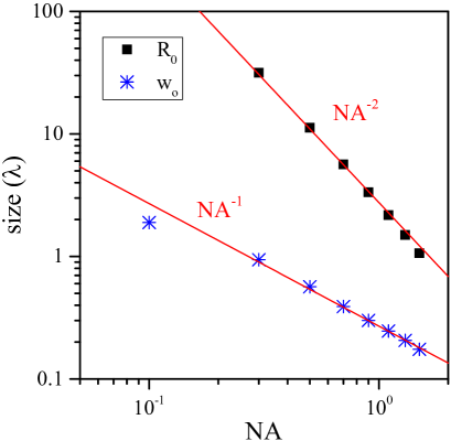
Figure S4: Calculated dependence of the coefficient $R_{0}$ in the focal plane (solid squares) on the objective numerical aperture, using a filling factor $\beta=0.83$ as in the experiment in a medium of $n=1.5185$. The Gaussian width $w_{0}$ for the in-plane distribution of $A_{\rm FWM}^{+}$ is also shown (stars). Sizes are in unit of wavelength ($\lambda$). Red lines show linear and quadratic dependencies on $1/{\rm NA}$ as indicated.

As described in the previous section and in the manuscript, the four-wave mixing amplitude ratio $A_{\rm FWM}^{-}/A_{\rm FWM}^{+}$ scales quadratically with the radial coordinates $R$ (for small values of $R$), such that in first approximation this coordinate can be calculated as $R=R_{0}\sqrt{A_{\rm FWM}^{-}/A_{\rm FWM}^{+}}$. Fig. S4 shows the dependence of the parameter $R_{0}$ in the focal plane ($z=0$) on the objective numerical aperture using a filling factor $\beta=0.83$ as in the experiment, and in a medium of $n=1.5185$. We find that $R_{0}$ scales quadratically with $1/{\rm NA}$. The width $w_{0}$ for the in-plane distribution of $A_{\rm FWM}^{+}$ fitted as a Gaussian function using the curvature near the center, i.e. $A_{\rm FWM}^{+}=A_{0}e^{-(R/w_{0})^{2}}$, is also shown, representing an effective point-spread function which scales linearly with $1/{\rm NA}$.

vi Amplitude and phase of FWM ratio versus particle ellipticity

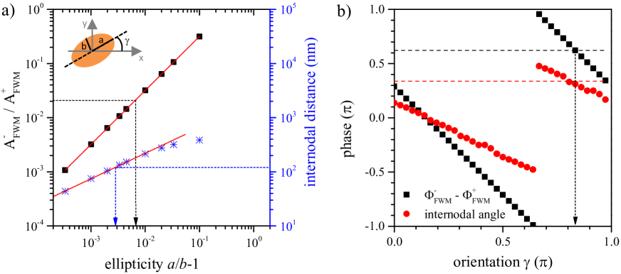
Figure S5: Calculated dependencies of the amplitude and phase of the cross to co-circularly polarised FWM ratio $E_{\rm FWM}^{-}/E_{\rm FWM}^{+}$ in the focal plane versus nanoparticle ellipticity and orientation. a) FWM ratio amplitude $A_{\rm FWM}^{-}/A_{\rm FWM}^{+}$ in the focus center (left axis) and distance between the two displaced amplitude minima (right axis) versus particle ellipticity $a/b-1$. b) Phase of the FWM ratio $\Phi_{\rm FWM}^{-}-\Phi_{\rm FWM}^{+}$in the focus center (squares) and angle of the internodal axis relative to the $x$-axis (circles). Dashed lines show the experimental values from Fig. 4 in the main text. The inset in (a) shows a sketch of the elliptical nanoparticle with long (short) semi-axis $a$ ($b$), and orientation angle $\gamma$.

Although being a limitation to achieve nanometric position accuracy, it is remarkable how sensitive the described FWM technique is to particle asymmetry, which could be used as a new tool to detect particle ellipticity down to $10^{-4}$ (corresponding to atomic accuracy comparable to TEM) as well as particle orientation. This is shown in Fig. S5. The FWM amplitude ratio in the focus center scales linearly with the particle ellipticity $a/b-1$ (where we assumed $b=c$ and $a$, $b$ and $c$ aligned along the $x$, $y$ and $z$ axis respectively). Furthermore the distance between the two displaced amplitude minima scales with the square root of the ellipticity. Fig. S5a shows these dependencies (red lines) and the experimental values (dashed lines) observed in Fig. 4 of the main manuscript, which indicate an ellipticity of about 0.5%. The occurrence of higher order modes in the measured data could also be used with appropriate modelling (beyond the the Rayleigh regime) to determine more details about the specific shape of the measured particle. Fig. S5b shows that the finite value of the phase of the FWM ratio in the focus center is given by -2$\gamma$ plus an offset, with the particle orientation angle $\gamma$ defined as the angle between the longer particle axis and the $x$-axis (see sketch in Fig. S5). Conversely, this phase is almost independent on the ellipticity (see Fig. S6). Furthermore, the orientation angle of the internodal axis relative to the $x$-axis scales as -$\gamma$ (plus an offset). Dashed lines show the experimental values from Fig. 4 of the main manuscript which indicate that the particle was oriented with $\gamma$ of about $150^{\circ}$.

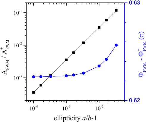
Figure S6: Calculated cross to co-circularly polarised FWM ratio amplitude and phase in the focus center versus nanoparticle ellipticity, for a particle orientation angle $\gamma=150^{\circ}$.

vii Polarisability resulting in an $l=1$ optical vortex of the cross-circularly polarised FWM

Firstly, we note that for a circularly polarized incident field, the longitudinally polarized field component ($E_{\rm z}$) in the focal plane exhibits an $l=1$ optical vortex, while the cross-circularly polarized component is an $l=2$ vortex. This is shown in Fig. S7 for the case of a 1.45 NA objective, as calculated in the main manuscript in Fig. 1b.

In order to reproduce the experimental findings in Fig. 6a of the main manuscript, we assumed a particle polarisability tensor representing a rotationally-averaged elliptical particle (hence an effectively spherical particle with equal semiaxis) plus a contribution coupling the longitudinal field component into the $(x,y)$ plane. Therefore, the particle polarisability tensor was described as:

$$\hat{\alpha}=\alpha_{0}\left(\begin{matrix}1&0&0\\ 0&1&0\\ 0&0&1\end{matrix}\right)+C\alpha_{0}\left(\begin{matrix}0&0&1\\ 0&0&0\\ 1&0&0\end{matrix}\right)$$ (S4)

with $\alpha_{0}$ given by Eq. S1 for $a=b=c=25$ nm in a surrounding medium consisting of water with index $n=\sqrt{\epsilon_{\rm m}}=1.333$, and $C$ being a complex coefficient, the amplitude of which was adjusted to reproduce the strength of the FWM amplitude ratio in the experiment (for the calculations in Fig. 6c we used $|C|$=0.37).

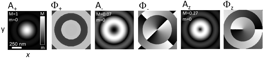
Figure S7: Calculated field distribution in the focal plane of a 1.45 NA objective for an incident field left ($\sigma^{+}$) circularly polarized, using a filling factor $\beta=0.83$ as in the experiment. $A_{+}$, $A_{-}$ and $A_{\rm z}$ are the co-circular, cross-circular and longitudinally polarised amplitudes, and $\Phi_{+}$, $\Phi_{-}$, and $\Phi_{\rm z}$ the corresponding phases. Linear grey scale from $-\pi$ to $\pi$ for phases, and from $m$ to $M$ for field amplitudes, as indicated

S2 Experiments

i Gold nanoparticles attached onto glass

Before use, glass slides and coverslips were cleaned from debris. Cleaning was performed first with acetone and high-quality cleanroom wipes, followed by a chemical etch called Caro’s etch, or more commonly, Piranha etch. The investigated samples were nominally spherical gold NPs of 30 nm and 5 nm radius (BBI Solutions) drop cast onto a glass coverslip, covered in silicon oil (refractive index $n=1.518$) and sealed with a glass slide. Examples of transmission electron microscopy (TEM) images of these NPs are shown in Fig. S8.

ii Gold nanoparticles in agarose gel

Before use, glass slides and coverslips were cleaned with acetone. 500 mg of agar powder (high molecular biology grade agarose, Bioline Cat. 41025) was placed in a conical glass beaker filled with 10 mL of pure water, and the mixture was boiled in a microwave for about 60 s until a homogeneous liquid was formed. Nominally spherical gold NPs of 25 nm radius (BBI Solutions) in pure water were added to the mixture to achieve a typical concentration of $10^{9}$ NPs/mL. A chamber was formed by attaching an adhesive imaging spacer of 0.12 mm thickness with a 13 mm diameter hole (GraceBioLabs) onto a glass coverslip. 20 ${\mu}$L volume of the gold NP agar mixture was pipetted into the chamber and sealed with a glass slide.

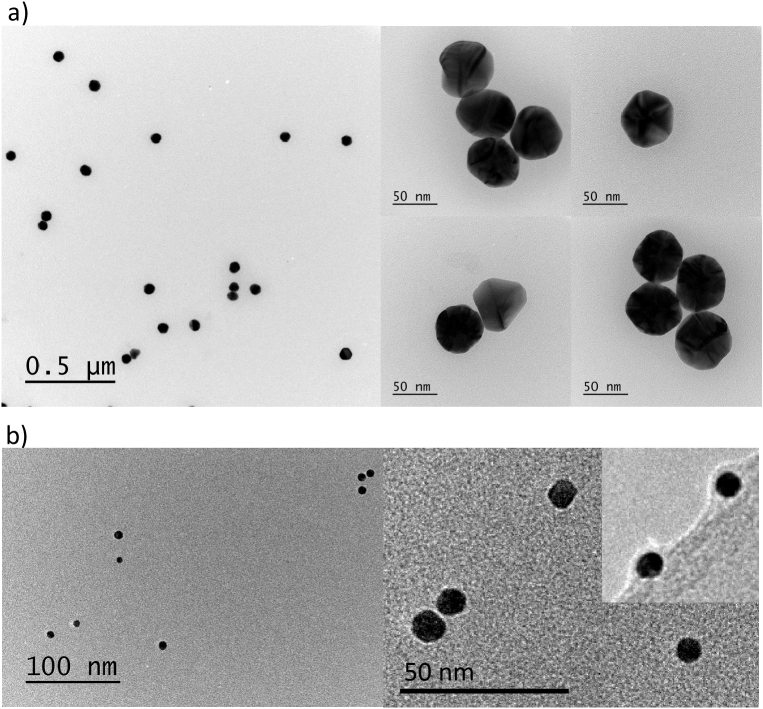
Figure S8: Transmission electron microscopy of nominally spherical 30 nm radius (a), and 5 nm radius (b) gold nanoparticles.

iii Gold nanoparticles in fixed cells

HeLa cells were seeded onto gridded coverslips and then loaded with 20 nm radius gold NPs via clathrin mediated endocytosis, using the transferrin (Tf) ligand attached onto the NP via a biotin-streptavidin conjugate. Tf-biotin was purchased from Sigma Aldrich and 20 nm radius gold NPs covalently bound to streptavidin were purchased from Innova Biosciences. Cells were placed on ice for 10 min to inhibit endocytosis, incubated with 50 $\mu$g/mL Tf-biotin in ice-cold serum-free medium for 8 min and then washed 3 times in ice-cold phosphate-buffered saline (PBS) at pH 7.4. Cells were then incubated with a dilution of gold NP-streptavidin conjugate in ice-cold serum-free medium, followed by washing 3 times in PBS pH 7.4. Cells were subsequently incubated in pre-warmed imaging medium for 6 hours to enable endocytosis, and then fixed in 3% paraformaldehyde for 10 mins at room temperature. They were washed 3 times in PBS at room temperature and mounted onto a glass slide using a DAKO (Dako UK Ltd) mounting medium at 80%.

iv Lock-In detection of the modulation

A digital lock-in amplifier Zurich Instruments HF2LI was used to detect the FWM signal at both sidebands $\nu_{2}\pm\nu_{\rm m}-\nu_{\rm L}=(2\pm 0.4)$MHz together with the reflected probe at the carrier $\nu_{\rm c}=\nu_{2}-\nu_{\rm L}=2$MHz ($\nu_{2}=$82 MHz is the frequency up-shift of the probe field via AOM₂, $\nu_{\rm m}=0.4$ MHz is the intensity modulation of the pump via AOM₁, and $\nu_{\rm L}=80$ MHz is the pulsed laser repetition rate, see also Fig. 1 in main paper). To produce a modulation of the pump intensity, we supplied a modulation at $\nu_{\rm m}$ to the digital input of the AOM₁ driver (Intraaction DFE-834C4-6), generated by the internal oscillator of the lock-in. To provide an electronic reference to the lock-in at the carrier frequency of 2 MHz, we assembled an external electronic circuit using coaxial BNC components (Minicircuits), mimicking the optical mixing. The laser repetition frequency was taken from the 80 MHz photodiode signal output of the Ti:Sa laser (Newport/Spectra Physics MaiTai). After filtering for the first harmonics using a 50 MHz high pass (BHP-50+) and a 100 MHz low-pass (BLP-100+), the signal was mixed with the frequency $\nu_{2}$ from the +10dBm reference output of the AOM₂ driver (Intraaction DFE-774C4-6) using an electronic mixer (ZP-1LH+) and a 10 MHz low pass filter (BLP-10.7+) to produce an electric sine wave at the difference frequency $\nu_{2}-\nu_{\rm L}=2$ MHz. The latter was then converted from sine to TTL using a comparator (Pulse Research Lab - PRL-350TTL-220), to be suited as external reference for the HF2LI using the DIO0 input (the two available high-frequency analog inputs were used for the two balanced-diode signals).

To discuss the analysis of the dual sideband detection by the lock-in, we start by describing the detected voltage of the balanced-diode signal as the real part of

$$U=a_{\rm c}e^{i\omega_{\rm c}t}\left(1+a_{\rm m}\cos(\omega_{\rm m}t+\varphi)\right).$$ (S5)

with the complex carrier amplitude $a_{\rm c}$, which is measured directly by the ZI-HF2LI via the in-phase ($Re$) and in-quadrature ($Im$) components at the carrier frequency $\nu_{\rm c}=\omega_{\rm c}/(2\pi)$, and the complex relative modulation of the carrier $a_{\rm m}$ with the frequency $0<2\pi\nu_{\rm m}=\omega_{\rm m}<\omega_{\rm c}$ and the phase $\varphi$. The modulation is due to the intensity modulation of the pump field, which is a real quantity and can thus be described by a cosine. This can be rewritten as

$$U=a_{\rm c}e^{i\omega_{\rm c}t}+\frac{a_{\rm c}a_{\rm m}}{2}e^{i\varphi}e^{i(\omega_{\rm c}+\omega_{\rm m})t}+\frac{a_{\rm c}a_{\rm m}}{2}e^{-i\varphi}e^{i(\omega_{\rm c}-\omega_{\rm m})t}.$$ (S6)

Accordingly, the complex amplitudes of the lower and upper sidebands are $a_{\pm}=a_{\rm c}a_{\rm m}e^{\pm i\varphi}/2$, which are detected together with $a_{\rm c}$ by the ZI-HF2LI using the dual sideband modulation detection. The modulation phase $\varphi$ can be determined modulo $\pi$ by

$$e^{2i\varphi}=\frac{a_{+}}{a_{-}}$$ (S7)

and is due to the delay $\tau$ between the modulation output of the lock-in and the detection of the amplitude modulation by the lock-in, specifically $\varphi=-\omega_{\rm m}\tau$, resulting in the modulation term $\cos(\omega_{\rm m}(t-\tau))$. The modulation of the detected probe field, which is the FWM signal, is given by

$$a_{\rm c}a_{\rm m}=a_{+}e^{-i\varphi}+a_{-}e^{i\varphi}$$ (S8)

The determination of $\varphi$ modulo $\pi$ leads to an uncertainty of the sign of the modulation. The phase shift $\varphi$ can be determined including its sign by directly detecting the reflected pump beam which is frequency up-shifted via AOM₁ by the amount $\nu_{1}=83$ MHz, using $\nu_{1}-\nu_{\rm L}$ instead of $\nu_{2}-\nu_{\rm L}$ in the lock-in reference, and knowing that $a_{\rm m}>0$. Since the phase shift is given by electronic and acousto-optic delays it is stable to a few degrees. Once $\varphi$ is known, the four-wave mixing field $a_{\rm m}a_{\rm c}$ is determined using Eq.(S8).

v Shot-noise limited detection: Dependence on reference power

Figure S9: Standard deviation $\sigma$ of the distribution of the measured FWM field (in-phase $Re$ component, cross-circularly polarized) in a spatial region away from the particle, as a function of the total power in the reference beam. 1 ms pixel dwell time. A fit to the data is shown as indicated

The experimental noise was evaluated by taking the statistical distribution of the measured FWM field (in both $Re$ and $Im$ components) in a spatial region away from the particle where no detectable signal is present. The standard deviation $\sigma$ of this distribution was deduced for each component. For the measurement conditions as in Fig. 4 in the main paper, $\sigma$ was found to be the identical in the $Re$ and $Im$ component, and for the co-polarised and cross-polarised components, as expected for an experimental noise given by the shot-noise of the reference beam and the electronic noise. Fig. S9 shows $\sigma$ as a function of the total power $P_{\rm R}$ of the reference beam entering the balanced detector, which is split onto the 4 photodiodes (Hamamatsu S5973-02) of the dual-polarization balanced detector with a transimpedance of $10^{4}$ V/A. It shows a noise at a frequency of 2 MHz and 1 ms integration time of $\sigma_{0}\sqrt{1+P_{\rm R}/P_{\rm el}}$, with the electronic noise of $\sigma_{0}=3.2\,\mu$eV, equivalent to the shot noise created by $P_{\rm el}=1.85$ mW at the detector input, and is thus shot-noise limited for $P_{\rm R}>P_{\rm el}$. We used $P_{\rm R}\sim 3\,$mW in the experiments shown.

vi Pump-induced change of particle polarisability: Pump power and delay dependence

An example of the co-polarised FWM field amplitude $A_{\rm FWM}^{+}$ for a 30 nm radius NP at the focus center as a function of the pump-probe delay time and power is shown in Fig.S10.

As discussed in detail in our previous work MasiaPRB12 , the pump-probe delay dependence reflects the transient change of the electron and lattice temperature following the absorption of the pump pulse by the nanoparticle. As a result of the ultrafast heating of the electron gas, the pump-induced change of the particle polarisability, and in turn the transient FWM field amplitude, reaches its maximum at a pump-probe delay $\tau$ of about 0.5 ps. The subsequent decay on a picosecond time scale reflects the thermalization with the lattice, i.e. the cooling of the electron gas via electron-phonon coupling.

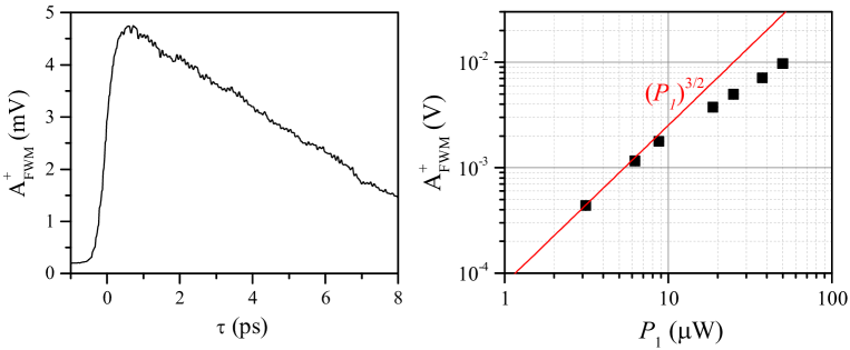
Figure S10: Left: Co-polarised FWM field amplitude for a 30 nm radius NP at the focus center versus pump-probe delay time $\tau$ for a pump (probe) power at the sample of 40 ${\mu}$W (20 ${\mu}$W). Right: Co-polarised FWM field amplitude at the focus center versus versus pump power at $\tau=0.5$ ps. The probe power is half the pump power. The scaling $\propto P_{1}^{3/2}$ expected in the third-order regime is shown.

The scaling of $A_{\rm FWM}^{+}$ at $\tau=0.5$ ps with increasing pump and probe power shown in Fig. S10 follows the expected third-order nonlinear behavior for small powers, and the onset of saturation at higher power. Pump power ($P_{1}$) and probe power ($P_{2}$) were increased while keeping a constant ratio $2P_{2}=P_{1}$. At small powers, in the limit of a pump-induced change of the particle polarisability linear with the pump intensity, the FWM field amplitude scales as $P_{1}\sqrt{P_{2}}\propto P_{1}^{3/2}$.

vii Background-free FWM detection in cells

To exemplify that our FWM detection is very specific to gold NPs and free from background even in highly scattering and fluorescing environments, Fig. 3 in the main manuscript shows HeLa cells that have internalized 20 nm radius gold NPs bound to the transferrin receptor, via clathrin mediated endocytosis. Cells were fixed (with 3% paraformaldehyde solution) onto gridded glass coverslips, and immersed in a mounting medium (80% Dako) chambered with a glass slide. They were imaged with FWM using the $100\times$ magnification 1.45 NA oil-immersion objective specified in the main manuscript. Differential interference contrast (DIC) microscopy was also available in the same instrument, with wide-field illumination via an oil condenser of 1.4 NA and detection with a sCMOS camera (Pco.edge 5.5).

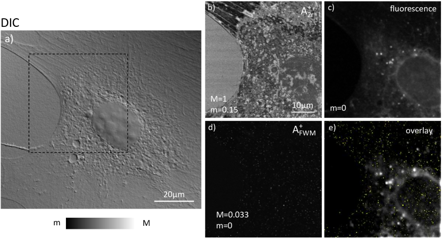
Figure S11: Fixed 3T3 cells that have internalized gold NPs of 10 nm radius imaged by (a) differential interference contrast (DIC) microscopy, (b) co-circularly polarised reflection amplitude $A_{\rm 2r}^{+}$, (c) confocal epi-fluorescence, (d) co-circularly polarised FWM amplitude $A_{\rm FWM}^{+}$. Amplitude scales from m to M are indicated (for confocal fluorescence M$=1.37\times 10^{6}$ (photoelectrons/sec)). FWM was acquired with pump-probe delay time of 0.5 ps, pump (probe) power at the sample of 60 $\mu$W (30 $\mu$W), 0.4 ms pixel dwell time, pixel size in plane of 63 nm and z-stacks over 3 $\mu$m in 500 nm z-steps. FWM is shown as a maximum intensity projection over the z-stack, while the reflection and fluorescence images are on a single $(x,y)$ plane (scanning the sample position). e) is a false color overlay of the FWM (yellow) and fluorescence images in c) and d) respectively, brightness and contrast enhanced for visualization purposes.

Notably, FWM acquisition can be performed simultaneously with confocal fluorescence microscopy for correlative co-localisation analysis. An example of this simultaneous acquisition is shown in Fig. S11. Confocal epi-fluorescence detection was implemented in the same microscope set-up, by conjugating the sample plane onto a confocal pin-hole of adjustable opening in front of a photomultiplier detector (Hamamatsu H10770A-40). Excitation occurred via the same laser beam used for FWM; fluorescence was collected via the same objective (in this case 1.45 NA oil-immersion) and spectrally separated using a dichroic beam splitter for pick-up and a bandpass filter transmitting in the 600-700 nm wavelength range in front of the photomultiplier. Fig. S11 shows 3T3 cells loaded with 10 nm radius gold NPs using a protocol similar to the one described above for HeLa cells. Fixed cells were image with DIC, reflection, FWM and simultaneous confocal fluorescence. The co-circularly polarized reflection image $A_{\rm 2r}^{+}$ in Fig. S11b correlates with the cell contour seen in DIC in the region highlighted by the dashed frame, and shows a spatially varying contrast due to thickness and refractive index inhomogeneities in the sample. Epi-fluorescence in Fig. S11c correlates with the cell morphology seen in DIC and reflection image, and is dominated by autofluorescence near the cell nucleus. The co-circularly polarised FWM amplitude $A_{\rm FWM}^{+}$ shown in Fig. S11d is a maximum intensity projection over a 3 ${\mu}$m $z$-stack and clearly indicates the location of single gold NPs in the cell. FWM imaging is background-free (throughout the $z$-stack) despite the significant scattering and autofluorescing cellular contrast seen in Fig. S11a,b,c. Fig. S11e shows a false color overlay of the FWM and fluorescence image.

viii FWM field images of various particles

Fig. S12 gives examples of the measured FWM field ratio $E_{\rm FWM}^{-}/E_{\rm FWM}^{+}$ in amplitude and phase in the focal plane for different NPs of nominally spherical 30 nm radius, showing a variety of patterns in terms of the amplitude and phase in the focus center, the position of the amplitudes nodes, their distance and orientation and the angular distribution of the ratio phase. Fig. S12a is an overview while Fig. S12b-e are higher resolution zooms over individual NPs. The heterogeneity of the observed patterns is consistent with the heterogeneous NP shape and asymmetry observed in TEM.

Figure S12: Measured FWM ratio amplitude and phase as a function of NP position in the focal plane on various nominally spherical 30 nm radius single gold nanoparticles. Grey scale is from $-\pi$ to $\pi$ for all phases. Amplitude ratio is in logarithmic scale over 3 orders of magnitudes from 0.01 to 10. Reference power was 2.6 mW. Pump-probe delay time was 0.5 ps. Pump (probe) power at the sample was 24 $\mu$W (12 $\mu$W) for (a)-(c), 8 $\mu$W (4 $\mu$W) for (d), and 18 $\mu$W (9 $\mu$W) for (e). Pixel dwell time was 0.5 ms for (a) and 3 ms for (b)-(e). Pixel size in plane was 32 nm for (a), 17 for (b) and 10 nm for (c)-(e).

ix FWM measurements on 5 nm radius nanoparticles

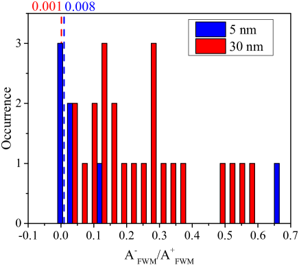
Figure S13: Histogram of the occurrence of the FWM amplitude ratio $A_{\rm FWM}^{-}/A_{\rm FWM}^{+}$ measured on nominally spherical 5 nm and 30 nm radius gold NPs in the focus center, as indicated. Dashed lines show the shot-noise limit in the corresponding experiments. For the 5 nm radius NPs, measurements were performed typically with 90 ${\mu}$W (45 ${\mu}$W) pump (probe) power at the sample, 10 ms pixel dwell time, 10 nm pixel size. FWM ratios (and corresponding shot-noise) were calculated by spatial averaging over an effective area of $9\times 9$ pixels. For the 30 nm radius NPs, measurements were performed with 24 ${\mu}$W (12 ${\mu}$W) pump (probe) power at the sample, 0.5 ms pixel dwell time, 32 nm pixel size. FWM ratios (and corresponding shot-noise) were calculated by spatial averaging over an effective area of $3\times 3$ pixels.

The FWM amplitude ratio $A_{\rm FWM}^{-}/A_{\rm FWM}^{+}$ in the focus center was measured on nominally spherical 5 nm radius gold NPs of the type shown in Fig. S8b, and compared with the ratio obtained on nominally spherical 30 nm radius gold NPs of the type shown in Fig. S8a. The results are summarized in Fig. S13. The shot-noise limit $\sigma/A_{0}$ in these experiment is indicated by the dashed lines. Notably, we observe that for the 5 nm radius NPs, a large proportion ($\sim 70\%$) has a FWM amplitude ratio $A_{\rm FWM}^{-}/A_{\rm FWM}^{+}\leq 0.02$ in the center of the focal plane, in this case limited by the signal-to-noise ratio rather than the particle asymmetry. Conversely, almost all NPs of nominal 30 nm radius have $A_{\rm FWM}^{-}/A_{\rm FWM}^{+}>0.02$ which is well above the shot-noise limit and is due to the particle asymmetry.

x Parameters for position localisation of a freely rotating single NP

Figure S14: Left: Axial dependence of the phase of the co-polarised FWM component (black) together with a linear fit (red line) having the slope $\partial z/\partial\Phi=37$ nm/rad. Middle: Radial dependence of the cross to co-polarised FWM amplitude ratio at the focal plane $z=0$. The red solid line shows a fit assuming the linear dependence $R/R_{0}=A_{\rm FWM}^{-}/A_{\rm FWM}^{+}$ with $R_{0}=1.33\,\mu$m at the focal plane. Right: Phase of the cross to co-polarised FWM ratio $\Theta=\Phi_{\rm FWM}^{-}-\Phi_{\rm FWM}^{+}$ versus polar angle in the $z=0$ plane, following the relationship $-\varphi=\Theta-\Theta_{0}$. The red solid line shows a fit using $\Theta_{0}=0.22$.

From the measurements on a freely rotating NP in an agarose gel shown in the main manuscript in Fig. 6 we have deduced the relationship between the FWM amplitude ratio $A_{\rm FWM}^{-}/A_{\rm FWM}^{+}$ and phase $\Phi_{\rm FWM}^{-}-\Phi_{\rm FWM}^{+}$ and the position coordinates in the focal plane, as measured from the sensor positions in the scanned piezoelectric sample stage. This is shown in Fig. S14. The $(x,y)$ experimental scans in Fig. 6 were first converted in 2D images along the polar coordinates $R$, $\varphi$. The data for $A_{\rm FWM}^{-}/A_{\rm FWM}^{+}$ were averaged over the full range of the $\varphi$ coordinate to obtain the one-dimensional dependence versus $R$ shown in Fig. S14. Similarly, the data for $\Phi_{\rm FWM}^{-}-\Phi_{\rm FWM}^{+}$ were averaged in $R$ over a region of about $60$ nm $<R<100$ nm to obtain the dependence versus $\varphi$. The FWM field phase $\Phi_{\rm FWM}^{+}$ versus $z$ also shown in Fig. S14 was taken from rapid 3D scans. We find that $\Phi_{\rm FWM}^{+}$ varies linearly with $z$, as discussed in Section S1.iv, with the slope $\partial z/\partial\Phi=37$ nm/rad (note that the experiments in the main manuscript in Fig. 6 were performed using a 1.27 NA water-immersion objective). We also find that $A_{\rm FWM}^{-}/A_{\rm FWM}^{+}$ has a simple linear dependence in $R$ given by $R/R_{0}=A_{\rm FWM}^{-}/A_{\rm FWM}^{+}$ with $R_{0}=1.33\,\mu$m in the focal plane. Moreover, the phase of the cross to co-polarised FWM ratio $\Theta=\Phi_{\rm FWM}^{-}-\Phi_{\rm FWM}^{+}$ versus polar angle follows the relationship $-\varphi=\Theta-\Theta_{0}$ with $\Theta_{0}=0.22$ for the data shown in Fig. S14.

xi Axial fluctuations of a rotating single NP encaged in an agarose gel pocket

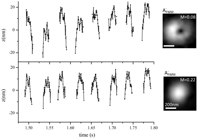
Figure S15: Time traces of the NP axial position coordinate retrieved from the measured $\Phi_{\rm FWM}^{+}$ during the scan corresponding to the distribution of the cross-circularly polarized FWM amplitude $A_{\rm FWM}^{-}$ shown in the inset. Images are on a linear grey scale from 0 to $M$, with $M$ given relative to the maximum $A_{\rm FWM}^{+}$. Pump (probe) power at the sample was 70 ${\mu}$W (10 ${\mu}$W); the focused size of the pump beam is twice larger than the probe in this experiment. Measurements were performed with 0.5 ms pixel dwell time, 0.5 ps pump-probe delay time, and 13 nm pixel size in-plane.

We investigated the fluctuations in the axial position coordinate retrieved from the phase $\Phi_{\rm FWM}^{+}$ of the co-circularly polarised FWM during a scan giving rise to an $l=1$ optical vortex in the cross-circularly polarized FWM (as shown in the main manuscript in Fig. 6b) in comparison with those observed during a scan where the highest value of $A_{\rm FWM}^{-}$ in the focus is measured. This is shown in Fig. S15. The behaviour is quite similar on both traces, dominated by systematic effects in the $z$ coordinate due to a cross-coupling to the $xy$ scanning, and a slow drift in $z$ – note that the $z$ range shown is only 50 nm. Superimposed, we find random variations in $z$ which are larger than the shot noise (estimated to be $\leq 3$ nm under the experimental conditions in Fig. S15). Based on our calculation of the effect of NP asymmetry on the cross-circularly polarized FWM (see also section S1.vi), the trace corresponding to the large $A_{\rm FWM}^{-}$ is attributed to the NP not rotating but stuck in a position where the NP ellipticity determines $A_{\rm FWM}^{-}$ in the focus center (from which we estimate the NP ellipticity to be $a/b-1=0.08$). For the trace corresponding to the observation of the $l=1$ mode in $A_{\rm FWM}^{-}$, we do observe larger jumps in the $z$-coordinate and the range spanned is slightly larger, consistent with the idea that the NP is freely rotating in 3D in this case, and hence also bouncing about within the agarose gel pocket in which it is trapped.

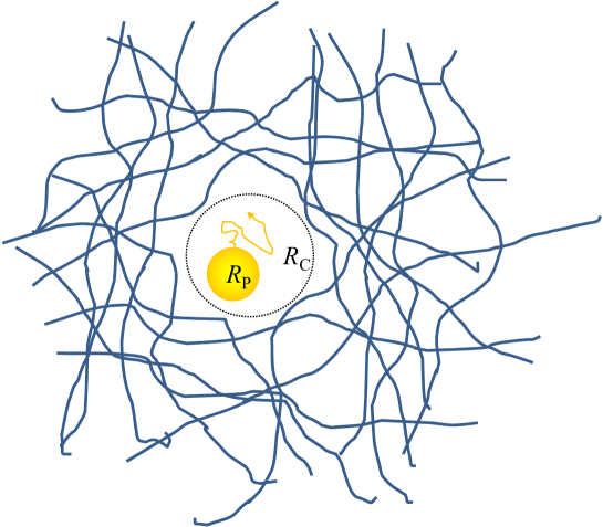
Figure S16: Sketch of the diffusion of a NP caged in a pocket of agar. The NP radius $R_{\rm P}$ and the cage radius $R_{\rm C}$ is indicated, together with a possible diffusion path.

To estimate the effect of restricted diffusion of a NP confined in a cage in agar, as sketched in Fig. S16, we assume a NP radius of $R_{\rm P}$ and a cage radius of $R_{\rm C}$. The free diffusion of the NP in water is given by

$$\langle x^{2}\rangle=2Dt=\frac{k_{\rm B}T}{3\pi\eta R_{\rm P}}t$$ (S9)

for each dimension of space, where $k_{\rm B}$ is Boltzmann’s constant, $T$ is the temperature, and $\eta$ is the dynamic viscosity of water. Here we are interested only in the $z$ coordinate. The boundary of the cage will limit this diffusion, confining the particle motion to a range $2(R_{\rm C}-R_{\rm P})$, which the particle explores in the characteristic time

$$\tau_{\rm C}=\frac{12\pi\eta R_{\rm P}(R_{\rm C}-R_{\rm P})^{2}}{k_{\rm B}T}$$ (S10)

If the measurement integration time $\tau$ is smaller than $\tau_{\rm C}$, the measured position fluctuation will explore the full cage size. If instead $\tau>\tau_{\rm C}$, the measured position will be an averaged position, with less fluctuations, an effect also known as motional narrowing. The standard deviation of the position fluctuations scales as the inverse root of the number of averages, hence is given by

$$\sigma=\frac{2(R_{\rm C}-R_{\rm P})}{\sqrt{12(1+\tau/\tau_{\rm C})}}$$ (S11)

where the $1/\sqrt{12}$ factor originates from the standard deviation of a uniform distribution. For the present measurements, we have $T=300\,$K, $\eta=1$ mPa$\cdot$s, $R_{\rm P}=25\,$nm, $\tau=0.5\,$ms. The resulting $\sigma$ as function of the cage radius is given in Fig. S17. We find that due to the motional narrowing, $\sigma$ is suppressed to below 5 nm for $R_{\rm C}\lesssim 45\,$nm, for which the NP has 40 nm space to move and thus also to rotate. The observed fluctuations in Fig. S15, which have a $\sigma$ in in the order of 5 nm, are therefore consistent with the assumption of free rotational diffusion.

Figure S17: Estimated standard deviation of the measured position of a NP of radius $R_{\rm P}=25\,$nm diffusing in a cage of radius $R_{\rm C}$ in water at room temperature for an integration time of $\tau=0.5\,$ms.

xii Randomly oriented non-rotating particle

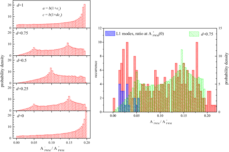
Figure S18: Left: Calculated histograms of the FWM ratio amplitude in the focus center for an asymmetric ellipsoid stuck in randomly oriented positions. The ellipsoid has semiaxis $a=b(1+e_{1})$ and $c=b(1+de_{1})$, with $e_{1}=0.0825$, and $d$ is varied as indicated. Right: Histogram of the FWM ratio amplitude in the focus center experimentally measured while repeatedly scanning over time a single 25 nm radius NP in agarose gel in the focal plane. The blue bars represent scans where an $l=1$ optical vortex was observed in the measurement of $A_{\rm FWM}^{-}$ with its node slightly off-centered, hence the finite non-zero value of $A_{\rm FWM}^{-}/A_{\rm FWM}^{+}$. Green bars are the calculated histogram shown in left for $d=0.75$.

We cannot reproduce the experimental finding of an $l=1$ optical vortex in the cross-circularly polarized FWM by assuming a non-rotating randomly-oriented asymmetric particle. This is shown in Fig. S18 where we have calculated the statistical distribution of the FWM ratio $A_{\rm FWM}^{-}/A_{\rm FWM}^{+}$ in the focus center assuming an asymmetric particle ellipsoid with axis $a=b(1+e_{1})$ and $c=b(1+de_{1})$ using the ellipticity $e_{1}=0.0825$ and considering random orientations in 3D. Note that by varying the parameter $d$ from 1 to 0 we change the particle shape from oblate to prolate. The histograms shown in Fig. S18 are significantly different from the experimentally observed one, the latter exhibiting a large occurrence of FWM ratios having values $A_{\rm FWM}^{-}/A_{\rm FWM}^{+}<0.05$ in the range where we see $l=1$ optical vortices. These calculations indicate that the experimental findings of an $l=1$ optical vortex in $A_{\rm FWM}^{-}$ cannot be attributed to a non-rotating asymmetric particle stuck in a randomly-oriented position.

xiii In situ calibration of in-plane particle position

Figure S19: Power spectrum of FWM field ratio not showing the 25 Hz oscillation imposed onto the sample stage for calibration, for the NP traces shown in the main paper Fig.7c-f.

For practical purposes, we implemented a simple way to achieve in situ calibration of the in-plane NP position coordinates without the need for prior knowledge and/or characterization of the particle optical response. This is achieved by applying a small oscillation of known amplitude (here 16 nm) at 25 Hz frequency to the $x$ axis of the sample stage, which is accurately measured by the position sensor in the stage. When the FWM field ratio from the NP encodes the NP in-plane position as discussed in the main manuscript, this oscillation is detected in the measured $E_{\rm FWM}^{-}/E_{\rm FWM}^{+}$. To find the amplitude $\widetilde{A}$ of this oscillation (as a complex number i.e. including its phase) we then Fourier transform $E_{\rm FWM}^{-}/E_{\rm FWM}^{+}$ and multiply it with a Gaussian filter centered at 25 Hz (with 0.5 Hz FWHM). We also Fourier transform the detected $x$ position sensor from the sample stage to deduce the corresponding complex amplitude $\widetilde{x}_{0}$. We can then calibrate $E_{\rm FWM}^{-}/E_{\rm FWM}^{+}$ in terms of NP in-plane positions as $X={\rm Re}((\widetilde{x}_{0}/\widetilde{A})E_{\rm FWM}^{-}/E_{\rm FWM}^{+})$ and $Y={\rm Im}((\widetilde{x}_{0}/\widetilde{A})E_{\rm FWM}^{-}/E_{\rm FWM}^{+})$.

Conversely, if a NP exhibits a FWM field ratio dominated by the shape asymmetry, we do no longer observe this oscillation in $E_{\rm FWM}^{-}/E_{\rm FWM}^{+}$. This case is shown in the paper in Fig.7c-f. The power spectrum for this case is shown in Fig. S19.

References

- (1) Betzig, E. & Trautman, J. K. Near-field optics: Microscopy, spectroscopy, and surface modification beyond the diffraction limit. Science 257, 189–195 (1992).
- (2) Sánchez, E. J., Novotny, L. & Xie, X. S. Near-field fluorescence microscopy based on two-photon excitation with metal tips. Phys. Rev. Lett. 82, 4014–4017 (1999).
- (3) Schuck, P. J., Fromm, D. P., Sundaramurthy, A., Kino, G. S. & Moerner, W. E. Improving the mismatch between light and nanoscale objects with gold bowtie nanoantennas. Phys. Rev. Lett. 94, 017402 (2005).
- (4) Rust, M. J., Bates, M. & Zhuang, X. Sub-diffraction-limit imaging by stochastic optical reconstruction microscopy (storm). Nature Methods 3, 793–795 (2006).
- (5) Betzig, E. et al. Imaging intracellular fluorescent proteins at nanometer resolution. Science 313, 1642–1645 (2006).
- (6) Hell, S. W. Far-field optical nanoscopy. Science 316, 1153–1158 (2007).
- (7) Fujiwara, T., Ritchie, K., Murakoshi, H., Jacobson, K. & Kusumi, A. Phospholipids undergo hop diffusion in compartmentalized cell membrane. The Journal of Cell Biology 157, 1071–1081 (2002).
- (8) Ueno, H. et al. Simple dark-field microscopy with nanometer spatial precision and microsecond temporal resolution. Biophysical Journal 98, 2014–2023 (2010).
- (9) Gu, Y., Di, X., Sun, W., Wang, G. & Fang, N. Three-dimensional super-localization and tracking of single gold nanoparticles in cells. Anal. Chem. 84, 4111–4117 (2012).
- (10) Ortega-Arroyo, J. & Kukura, P. Interferometric scattering microscopy (iscat): new frontiers in ultrafast and ultrasensitive optical microscopy. Phys. Chem. Chem. Phys. 14, 15625–15636 (2012).
- (11) Lasne, D. et al. Single nanoparticle photothermal tracking (snapt) of 5-nm gold beads in live cells. Biophysical J. 91, 4598–4604 (2006).
- (12) Lasne, D. et al. Label-free optical imaging of mitochondria in live cells. Opt. Express 15, 14184–14193 (2007). And references therein.
- (13) Masia, F., Langbein, W., Watson, P. & Borri, P. Resonant four-wave mixing of gold nanoparticles for three-dimensional cell microscopy. Opt. Lett. 34, 1816–1818 (2009).
- (14) Masia, F., Langbein, W. & Borri, P. Measurement of the dynamics of plasmons inside individual gold nanoparticles using a femtosecond phase-resolved microscope. Phys. Rev. B 85, 235403 (2012).
- (15) Bohren, C. F. & Huffman, D. R. Absorption and Scattering of Light by Small Particles (Wiley-VCH, 1998).
- (16) Miles, B. T. et al. Sensitivity of interferometric cross-polarization microscopy for nanoparticle detection in the near-infrared. ACS Photonics 2, 1705–1711 (2015).
- (17) Katz-Boon, H. et al. Three-dimensional morphology and crystallography of gold nanorods. Nano Letters 11, 273 (2011).
- (18) Taylor, A. B., Siddiquee, A. M. & Chon, J. W. M. Below melting point photothermal reshaping of single gold nanorods driven by surface diffusion. ACS Nano 8, 12071–12079 (2014).
- (19) Manzo, C. & Garcia-Parajo, M. F. A review of progress in single particle tracking: from methods to biophysical insights. Rep. Prog. Phys. 78, 124601 (2015).
- (20) Nasse, M. J. & Woehl, J. C. Realistic modeling of the illumination point spread function in confocal scanning optical microscopy. J. Opt. Soc. Am. A 27, 295–302 (2010).