Chiral symmetry and the properties
of hadrons in the Generalised Nambu–Jona-Lasinio model

Abstract

Various aspects of the Generalised Nambu–Jona-Lasinio model for QCD in four dimensions are reviewed. The properties of mesonic excitations are discussed in detail, with special attention paid to the chiral pion. The spontaneous chiral symmetry breaking in the vacuum and the effective chiral symmetry restoration in the spectrum of highly excited mesons and baryons are described microscopically.

1 Introduction

Quark models for strong interactions have a long history, starting from the mid of the previous century when the idea of hadrons, to be composed of quarks, was commonly accepted. And, as it happens, not only the number of various quark models, but even the number of their types turns out to be quite large. For example, the so-called Coulomb+linear potential model of [1] describes heavy quarkonium spectra with rather good accuracy, which is clearly due to the heavy quark mass being much larger than the scale of strong interaction $\Lambda_{\rm QCD}$. A naïve kinematical relativisation [2] of quark model allows one to consider mesons made of light quarks, though the justification of the potential model approach is less obvious in this case. The given approach, as well as similar models, is simple, also for numerical calculations, however its range of applicability is very limited, and many phenomena inherent to Quantum Chromodynamics (QCD), which are of interest for the phenomenology of strong interactions, cannot be addressed in such a framework. Among those one should mention the effect of spontaneous breaking of chiral symmetry in QCD vacuum, its implications in the spectrum of hadrons, and the effective restoration of chiral symmetry in excited hadrons.

It is well-known that, in the chiral limit, the $SU(2)_{L}\times SU(2)_{R}$ symmetry of QCD Lagrangian is broken, and this affects the observed spectrum of hadrons. Thus, the spontaneous symmetry breaking $SU(2)_{L}\times SU(2)_{R}\rightarrow SU(2)$ [3] manifests itself through the absence of low-lying hadrons populating multiplets of the $SU(2)_{L}\times SU(2)_{R}$ group, through the Goldstone nature of the pion, in particular, through its vanishing (beyond the strict chiral limit — finite but quite small compared to the typical hadronic scale) mass, through the nonzero value of the chiral condensate in the vacuum, and so on. Thus, chiral symmetry is realised nonlinearly in the low-lying hadrons.

Meanwhile, there are good reasons to believe that the aforementioned symmetry is effectively restored both in the spectrum of excited baryons [4, 5, 6] and excited mesons [7, 8, 9]. A nice and convincing justification of such a restoration in the spectrum of excited hadrons was suggested in a recent paper [10], where the masses of the light hadrons were extracted from the lattice configuration after the near-zero modes of the Dirac operator, responsible for the spontaneous chiral symmetry breaking [11], had been artificially removed from the latter. The resulting mass spectrum demonstrated a remarkably high degeneracy pattern, including formation of the chiral multiplets [12].

The full solution of QCD would yield a microscopic description of the effect of the spontaneous breaking of chiral symmetry. In the absence of a such solution, various approaches were suggested aimed at identification of gluonic field configurations which could be responsible for chiral symmetry breaking. It is quite natural to relate chiral symmetry breaking to confinement, yet another prominent feature of QCD. For example, in the approach of [13] confining kernel derived in the Vacuum Correlator Method [14] gives rise to the interaction of light quarks with Nambu-Goldstone fields, arriving in such a way at an effective chiral Lagrangian. The subject of the present review is a phenomenological approach which employs a simple ansatz for the confining kernel pertinent to the matter in hand. The approach gains experience from the ’t Hooft model [15] for two-dimensional QCD in the limit of the large number of colours ($N_{C}\to\infty$).

First, we notice that a microscopic description of the effect of the spontaneous breaking of chiral symmetry requires an intrinsically field theoretical approach which takes into account, within the very same formalism, both particles and antiparticles on equal footing. And this necessity lies outside the scope of constituent quark models as they merely provide an essentially quantum mechanical approach, even if one considers relativistic kinematics. Formally, the problems stems from the fact that, working in the formalism of relativistic quantum-mechanical Hamiltonians, one is stuck to a particular (positive) sign of the energy while the contributions from the other (negative) sign of the energy are neglected. Such “negative” solutions correspond to antiparticles, so that the interplay of both positive and negative solutions leads to the Z-like (Zitterbewegung) trajectory of the particle, that is, to the so-called $Z$-graphs. The problem can be traced down to the spectrum: the Salpeter equation that emerges for the bound states is defined with the help of a single-component Hamiltonian which describes the particle and, therefore, the resulting bound-state equation is derived curtailed of the full Hamiltonian components related to antiparticles. Such an approximation is well-justified for heavy particles, however it is obviously misleading for the light quarks and henceforth for the light hadrons built thereof — for the chiral pion in the first place.

The proper mechanism to account for the Zitterbewegung motion of particles can be established in terms of a matrix Hamiltonian and a two-component wave function. In [16] such an approach to the two-dimensional ’t Hooft model was suggested and described in detail. The key approximations which allowed one to control the pair creation process is the limit of the large number of colours, $N_{C}\to\infty$ (an introduction to this limit in QCD and related issues can be found in [17]). Also, it has to be noticed that the limit of the large number of degrees of freedom allows one to override [18] the Coleman’s no-go theorem which forbids spontaneous breaking of chiral symmetry in two dimensions [19]. Additional simplifications in the model arise from the instantaneous type of the interaction mediated by the two-dimensional gluon. To establish the latter property, it is sufficient to count the number of the degrees of freedom for the two-dimensional gluon and then to arrive straightforwardly at the absence of the gluon transversal propagating degrees of freedom. Then the ’t Hooft model in the axial gauge considered in [16] describes the interaction of two quark currents taken at equal time and mediated by the confining potential which depends on the one-dimensional interquark separation. The terms containing higher powers of the quark currents do not appear in this Hamiltonian, which is a reflection of the fact that all correlators of several gluonic fields either vanish or reduce to the powers of the bilocal correlator, which is nothing but the gluon propagator. As a result, there exists only one irreducible field correlator $\langle\langle A_{1}A_{2}\rangle\rangle=\langle A_{1}A_{2}\rangle-\langle A_{1}\rangle\langle A_{2}\rangle=\langle A_{1}A_{2}\rangle$ with all such irreducible correlators of higher orders vanishing. This result is exact in two dimensions and it does not rely on any approximations or assumptions. A review of the ’t Hooft model in the axial gauge can be found in [20].

In contrast to the two-dimensional case, the instantaneous nature of the interquark interaction and the absence in the Hamiltonian of the terms with the product of more than two quark currents are approximations that allow one to build a realistic quark model which we review in what follows. Thus, a quark model with quark currents endowed with an instantaneous interaction was suggested as a model for QCD about 30 years ago in [21, 22, 23, 24] and it was studied in detail in the Hamiltonian formalism in [25, 26, 27, 28, 29, 30], as well as in the later works [31, 32, 33, 34, 35]. As was mentioned above, this model can be regarded as the four-dimensional generalisation of the ’t Hooft model in two dimensions. At the same time, the same model can also be viewed as the generalisation of the four-dimensional Nambu-Jona-Lasinio (NJL) model [3] to a nonlocal interaction of the quark currents. It is important to notice that, in spite of its long history, the NJL model [3] still remains a useful and convenient tool for various studies in the physics of strong interactions. An important role for this to come true was played by a detailed study of the connection of the given model with QCD (see, for example, [36, 37]) and by its further developments (see the review papers [38, 39]) which allow one to extend considerably the spectrum of the problems where this model can be successfully employed. An important feature of the Nambu-Jona-Lasinio-type model, hereafter referred to as the Generalised Nambu-Jona-Lasinio (GNJL) model, is the presence of the confining interaction which allows one to employ this model to address the problem of bound states and which also brings in an intrinsic scale into the model.

The model is defined through the Hamiltonian (for simplicity, only one quark flavour is considered, generalisation to the multi-flavour case is trivial)

$$\hat{H}=\int d^{3}x\bar{\psi}({\bm{x}},t)\left(-i{\bm{\gamma}}\cdot{\bm{\bigtriangledown}}+m\right)\psi({\bm{x}},t)+\frac{1}{2}\int d^{3}xd^{3}y\;J^{a}_{\mu}({\bm{x}},t)K^{ab}_{\mu\nu}({\bm{x}}-{\bm{y}})J^{b}_{\nu}({\bm{y}},t),$$ (1)

where, as it was explained above, one has an interaction of the quark currents $J_{\mu}^{a}({\bm{x}},t)=\bar{\psi}({\bm{x}},t)\gamma_{\mu}\frac{\lambda^{a}}{2}\psi({\bm{x}},t)$ parametrised with the help of the instantaneous kernel

$$K^{ab}_{\mu\nu}({\bm{x}}-{\bm{y}})=g_{\mu 0}g_{\nu 0}\delta_{ab}V_{0}(|{\bm{x}}-{\bm{y}}|).$$ (2)

Hereinafter the following notations are used:

• low-case letters from the beginning of the greek (latin) alphabet, that is, $\alpha$, $\beta$ and so on ($a$, $b$ and so on) are used for the colour indices in the fundamental (adjoint) representation which run over $1,2\ldots N_{C}$ ($1,2\ldots N_{C}^{2}-1$);

• low-case letters from the middle of the greek alphabet ($\mu$, $\nu$ and so on) are used for the Lorentz indices which take values from 0 to 3;

• $\psi({\bm{x}},t)$ is the fermion (quark) field; $\bar{\psi}=\psi^{\dagger}\gamma_{0}$;

• $m$ is the mass of the quark (the chiral limit implies that $m=0$);

• $\gamma^{\mu}=(\gamma_{0},{\bm{\gamma}})$ are the Dirac matrices;

• $\lambda$ are the colour matrices (generators of the $SU(N_{C})$ group);

• $g_{\mu\nu}$ is the Minkowski metric tensor;

• $\delta_{ab}$ is the Kronecker symbol.

Typically, the confining potential is chosen in a power-like form,

$$V_{0}(|{\bm{x}}|)=K_{0}^{\alpha+1}|{\bm{x}}|^{\alpha},\quad 0\leqslant\alpha\leqslant 2,$$ (3)

where $K_{0}$ is the parameter of the model which has the dimension of mass. The qualitative predictions of the model are independent of the particular form of the potential, provided it should only be confining for coloured objects, on the one hand, and should demonstrate a moderate growth with the interquark separation to avoid divergent integrals, on the other.

The boundary cases with $\alpha=0$ and $\alpha=2$ require a special treatment. In particular, in the limit $\alpha\to 0$, the potential has to be re-defined as

$$\left.V_{0}(|{\bm{x}}|)\to{\tilde{V}}_{0}(|{\bm{x}}|)=K_{0}\frac{(K_{0}|{\bm{x}}|)^{\alpha}-1}{\alpha}\right|_{\alpha\to 0}=K_{0}\ln(K_{0}|{\bm{x}}|),$$ (4)

so that the resulting interaction is logarithmic. Strictly speaking, the potential can also be defined for negative values of $\alpha$ up to $\alpha>-1$ (for $\alpha=-1$, that is, for the Coulomb potential the integrals become divergent again (see [32] for the details)). However, the negative powers $\alpha$ do not provide confinement for the quarks, so they will be disregarded in what follows.

In the limit of $\alpha=2$ the Fourier transform of the potential reduces to the Laplacian of the three-dimensional $\delta$-function, so that, by taking integrals by parts one can turn all integral equations into second-order differential equations which are much simpler to deal with from the technical point of view. This explains why such a choice is quite popular in the literature (see, for example, [21, 22, 23, 24, 25, 26, 27, 28, 29]). Even larger values of $\alpha$, $\alpha>2$, lead to divergent integrals and are not considered (a detailed discussion of the problem can be found in [21, 22, 23, 32]). More realistic quantitative predictions can be made with the help of the linear confinement [40, 41, 42, 43, 44].

As was mentioned above, qualitative results are insensitive to the particular form of the potential, so that in most cases in what follows it will not be fixed. If, however, a quantitative investigation of equations is needed, the potential will be chosen in the most appropriate power-like form as given in equation (3).

The GNJL model meets a wide set of requirements, such as a) the ability to account for relativistic effects; b) the presence of an explicit confining force and, therefore, it can be employed to address various questions related to bound states of quarks, including excited hadrons; c) it is chirally symmetric (for $m=0$), d) it is able to describe the effect of the spontaneous breaking of chiral symmetry in the vacuum. The last point above deserves an additional remark. In particular, the given model fulfills all low-energy theorems such as the Gell-Mann-Oakes-Renner relation [45] (see [21, 22, 23]), the Goldberger–Treiman relation [46] (see [47]), the Adler self-consistency condition [48], and the Weinberg theorem [49] (see [50]). At the same time, the model possesses an attractive feature to describe microscopically the phenomenon of the spontaneous breaking of chiral symmetry in the vacuum and its effective restoration in the spectrum of excited hadrons. These questions are discussed in detail in the review. Furthermore, since the effects of the chiral symmetry breaking and restoration are closely related to the problem of the Lorentz nature of the confining interaction in quarkonia, the latter issue is also addressed in this review.

2 BCS approximation, mass-gap equation, and chirally broken vacuum

A convenient approach to studies of the model described by Hamiltonian (1) is the Bogoliubov-Valatin transformation which allows one to proceed from the “bare” quarks, which are the relevant degrees of freedom in the chirally symmetric vacuum, to the “dressed” quarks, which are the physical degrees of freedom in the chirally broken vacuum [25, 26, 27, 28, 29]. The quark field $\psi_{\alpha}({\bm{x}},t)$ is defined in terms of annihilation and creation operators $\hat{b}$, $\hat{d}$ and $\hat{b}^{\dagger}$, $\hat{d}^{\dagger}$, and takes the form

$$\psi_{\alpha}({\bm{x}},t)=\sum_{s=\uparrow,\downarrow}\int\frac{d^{3}p}{(2\pi)^{3}}e^{i{\bm{p}}{\bm{x}}}[\hat{b}_{\alpha s}({\bm{p}},t)u_{s}({\bm{p}})+\hat{d}_{\alpha s}^{\dagger}(-{\bm{p}},t)v_{-s}(-{\bm{p}})],$$ (5)

$$\left\{\begin{array}[]{rcl}u_{s}({\bm{p}})&=&\displaystyle\frac{1}{\sqrt{2}}\left[\sqrt{1+\sin\varphi_{p}}+\sqrt{1-\sin\varphi_{p}}\;({\bm{\alpha}}\hat{{\bm{p}}})\right]u_{s}(0),\\[8.53581pt] v_{-s}(-{\bm{p}})&=&\displaystyle\frac{1}{\sqrt{2}}\left[\sqrt{1+\sin\varphi_{p}}-\sqrt{1-\sin\varphi_{p}}\;({\bm{\alpha}}\hat{{\bm{p}}})\right]v_{-s}(0),\end{array}\right.$$ (6)

$$\hat{b}_{s}({\bm{p}},t)=e^{iE_{p}t}\hat{b}_{s}({\bm{p}},0),\quad\hat{d}_{s}(-{\bm{p}},t)=e^{iE_{p}t}\hat{d}_{s}(-{\bm{p}},0).$$ (7)

Here the rest-frame bispinors are defined as

$$u_{s}(0)=\left(\begin{array}[]{c}w_{s}\\ 0\\ \end{array}\right),\quad v_{-s}(0)=-i\gamma_{2}u_{s}^{*}(0)=\left(\begin{array}[]{c}0\\ i\sigma_{2}w_{s}^{*}\\ \end{array}\right),$$ (8)

where $\gamma_{2}(\sigma_{2})$ is the second Dirac(Pauli) matrix, $s=\pm 1$ labels the spin eigenstates, so that $(w_{s})_{i}=\delta_{si}$, $E_{p}$ is the dressed-quark energy. The quantity $\varphi_{p}$ which parametrises the Bogoliubov-Valatin transformation is known as the chiral angle and it is defined with the boundary conditions $\varphi_{p}(p=0)=\pi/2$ and $\varphi_{p}(p\to\infty)=0$.

Then, after the normal ordering in terms of the dressed creation and annihilation operators, Hamiltonian (1) takes the form

$$\hat{H}=E_{\rm vac}+:\hat{H}_{2}:+:\hat{H}_{4}:,$$ (9)

$$E_{\rm vac}[\varphi_{p}]=-\frac{1}{2}gV\int\frac{d^{3}p}{(2\pi)^{3}}\biggl{(}A_{p}\sin\varphi_{p}+B_{p}\cos\varphi_{p}\biggr{)},$$ (10)

where $V$ is the three-dimensional volume and the factor $g$ counts the total number of the degrees of freedom for each quark, $g=(2S+1)N_{C}$, where $2S+1$ with $S=1/2$ is the number of the quark spin projections (in the multi-flavour case, $g$ is to be additionally multiplied by the number of flavours $N_{f}$). The functions of the momentum $A_{p}$ and $B_{p}$ are given by the formulae

$$A_{p}=m+\frac{1}{2}\int\frac{d^{3}k}{(2\pi)^{3}}V({\bm{p}}-{\bm{k}})\sin\varphi_{k},\quad B_{p}=p+\frac{1}{2}\int\frac{d^{3}k}{(2\pi)^{3}}\;(\hat{{\bm{p}}}\hat{{\bm{k}}})V({\bm{p}}-{\bm{k}})\cos\varphi_{k},$$ (11)

where hats in $\hat{{\bm{p}}}$ and $\hat{{\bm{k}}}$ denote the unit vectors for the respective momenta (hats over scalar quantities identify the latter as operators — see, for example, (5)), $V=C_{F}V_{0}$ and $C_{F}=(N_{C}^{2}-1)/(2N_{C})$ is the eigenvalue of the fundamental Casimir operator. To ensure that the potential takes finite values in the limit $N_{C}\to\infty$, its strength is subject to an appropriate rescaling, that is, $K_{0}^{\alpha+1}N_{C}\underset{N_{C}\to\infty}{\to}\mbox{const}$.

The explicit form of the chiral angle $\varphi_{p}$ is determined from the requirement that the vacuum energy is kept to the minimum. For a qualitative investigation of the properties of the corresponding functional (10) it is convenient to use the following trick [30]. Suppose the given functional has a minimum at a particular function $\varphi_{0}(p)$. Then, if evaluated at a rescaled function $\varphi_{0}(p/\xi)$, with $0\leqslant\xi<\infty$, it must take larger values for all $\xi\neq 1$, and it should reproduce the above minimum at $\xi=1$. Finally, taking the limit $\xi\to 0$ is equivalent to taking an infinitely large argument of the chiral angle and, since $\varphi_{p}(p\to\infty)\to 0$, such a limit is equivalent to the evaluation of the energy functional for the trivial, chirally symmetric solution. Thus, it proves instructive to study the behaviour of the function $E_{\rm vac}(\xi)$ which should have a minimum at $\xi=1$. For simplicity, consider the chiral limit and set $m=0$. In this case, the only remaining dimensional parameter is the potential strength $K_{0}$. Then, by the redefinition of the integration variable in the functions $A_{p}$ and $B_{p}$, $p\to p/\xi$, one readily arrives at

$$E_{\rm vac}(\xi)=C_{1}\xi^{d+1}+C_{2}K_{0}^{\alpha+1}\xi^{d-\alpha},$$ (12)

where $D$ is the dimension of the space-time, $d=D-1$, while $C_{1}$ and $C_{2}$ are two $\xi$-independent constants. For convenience, let us count the energy from the chirally symmetric solution $\varphi_{p}\equiv 0$ which corresponds to $\xi=0$, that is, we set $E_{\rm vac}(0)=0$. Whether or not there exists a minimum with a negative energy at $\xi=1$ depends on the relation between the coefficients and the powers of the two contributions in expression (12). An interesting case is given by the limit $\alpha=d$. The ’t Hooft model for two-dimensional QCD constitutes an example of such a limit for which $\alpha=d=1$. Naively, one could expect that, in this limit, the second term in (12) turns to a constant, so that no nontrivial minimum can exist. However, this is not the case. It is important to notice that, for $\alpha=d$, the integrals in momentum are logarithmically divergent in the infrared and, as such, they need a regulator, hereinafter denoted as $\lambda$. Then, in the given limit, the second term in formula (12) contains a logarithmic dependence on $\xi$,

$$E_{\rm vac}^{(\alpha=d)}(\xi)=C_{1}\xi^{d+1}+C_{2}K_{0}^{d+1}\ln\left(\xi\frac{K_{0}}{\lambda}\right),$$ (13)

that entails two consequences: (i) a nontrivial minimum is possible, if the coefficients $C_{1}$ and $C_{2}$ have different signs and (ii) the vacuum energy grows as one approaches the trivial solution at $\xi=0$. In other words, the chirally symmetric phase of the theory ceases to exist [30]. A similar conclusion for the ’t Hooft model is made in [51].

Figure 1: Solution of the mass-gap equation (14) for $m=0$ and for the linear confining potential $V(r)=\sigma r$ where the parameter $\sigma$ has the dimension of the mass squared. The momentum $p$ is shown in the units of $\sqrt{\sigma}$.

For the Generalised Nambu-Jona-Lasinio model $d=3$, and in view of the restrictions for the value of the power $\alpha$ — see (3) — one always has $\alpha<d$. This ensures, for a particular choice of the signs of the coefficients $C_{1}$ and $C_{2}$ in (12), the existence of a nontrivial energetically favourable solution, as compared to the trivial vacuum. By a straightforward check, one can ensure that, indeed, the needed signs take place.

It should be noticed that the requirement that the vacuum energy should be a minimum guarantees at the same time that the quadratic part of the Hamiltonian, $:\hat{H}_{2}:$, is diagonal (that is, the anomalous terms of the form $\hat{b}^{\dagger}\hat{d}^{\dagger}-\hat{d}\hat{b}$ are missing), and the corresponding equation is known as the mass-gap equation [21, 22, 23, 24, 25, 26, 27, 28, 29],

$$A_{p}\cos\varphi_{p}=B_{p}\sin\varphi_{p}.$$ (14)

Then the dressed-quark dispersive law is

$$E_{p}=A_{p}\sin\varphi_{p}+B_{p}\cos\varphi_{p}.$$ (15)

It is easy to verify that the solution of the mass-gap equation for a free particle takes the form $\varphi_{p}=\arctan(m/p)$, and then the free dispersive law $E_{p}=\sqrt{p^{2}+m^{2}}$ is readily reproduced. It is also worthwhile mentioning that the same angle defines the Foldy-Wouthuysen transformation that brings the free Dirac Hamiltonian $H={\bm{\alpha}}{\bm{p}}+\beta m$ to the diagonal form $H^{\prime}=\beta E_{p}$. Such a deep connection between the chiral angle and the Foldy-Wouthuysen transformation persists for the nontrivial confining interaction and for the chiral angle given by the solution for the corresponding mass-gap equation (see, for example, [20, 33]).

For an arbitrary power-like confining potential (3), the mass-gap equation takes the form (in the chiral limit, that is, for $m=0$):

$$p^{3}\sin\varphi_{p}=\frac{1}{2}K_{0}^{3}\left[p^{2}\varphi^{\prime\prime}_{p}+2p\varphi_{p}^{\prime}+\sin 2\varphi_{p}\right],$$ (16)

for $\alpha=2$ [21, 22, 23, 24, 25, 26, 27, 28, 29], and

$$p^{3}\sin\varphi_{p}=K_{0}^{\alpha+1}\Gamma(\alpha+1)\sin\frac{\pi\alpha}{2}\int_{-\infty}^{\infty}\frac{dk}{2\pi}\left\{\frac{pk\sin[\varphi_{k}-\varphi_{p}]}{|p-k|^{\alpha+1}}+\frac{\cos\varphi_{k}\sin\varphi_{p}}{(\alpha-1)|p-k|^{\alpha-1}}\right\},$$ (17)

for $0\leqslant\alpha<2$ [32], where $\Gamma(\alpha+1)$ is the Euler Gamma function. For convenience and to make the formulae more compact, the absolute value of the momentum $p$ is formally prolonged to the domain $p<0$ according to the rule: $\cos\varphi_{-p}=-\cos\varphi_{p}$, $\sin\varphi_{-p}=\sin\varphi_{p}$. As was mentioned above, the mass-gap equation for the Harmonic Oscillator potential reduces to a second-order differential equation.

In Fig. 1, the behaviour of the chiral angle as a function of the momentum is exemplified by the solution of the mass-gap equation with the linear potential. Qualitatively, the shape of the curve does not depend on the particular form of the interquark potential. Further details of the formalism of the chiral angle can be found in [21, 22, 23, 24, 25, 26, 27, 28, 29, 30, 33], whereas the details of various studies of the mass-gap equation can be found in [32] (for the four-dimensional theory) and in [16, 52] (for the two-dimensional theory). In particular, in some of the works mentioned above it was pointed out that the mass-gap equation supports the existence of “excited” solutions, with the chiral angle possessing knots. Attempts to prescribe a physical meaning to such solutions can be found in [30, 31, 35]. In what follows, the problem of excited solutions (replicas) is not discussed, and we always refer to the chiral angle of the form depicted in Fig. 1 as to the nontrivial solution of the mass-gap equation.

For the chiral angle — solution of the mass-gap equation (14) Hamiltonian (9) takes a diagonal form [25, 26, 27, 28, 29],

$$\hat{H}=E_{\rm vac}+\sum_{\alpha=1}^{N_{C}}\sum_{s=\uparrow,\downarrow}\int\frac{d^{3}p}{(2\pi)^{3}}E_{p}[\hat{b}^{\dagger}_{\alpha s}({\bm{p}})\hat{b}_{\alpha s}({\bm{p}})+\hat{d}^{\dagger}_{\alpha s}(-{\bm{p}})\hat{d}_{\alpha s}(-{\bm{p}})],$$ (18)

and the contribution of the omitted term $:\hat{H}_{4}:$ is suppressed as $1/\sqrt{N_{C}}$ in the large-$N_{C}$ limit. In the literature, such an approximation is often referred to as the BCS approximation, in analogy with the similar approach by Bardeen, Cooper, and Schrieffer to the theory of superconductivity. The new, dressed, operators $b$ and $d$ annihilate the vacuum $|0\rangle$ which is related to the trivial vacuum $|0\rangle_{0}$, annihilated by the bare operators, through the following relations [25, 26, 27, 28, 29]:

$$|0\rangle=e^{Q-Q^{\dagger}}|0\rangle_{0},\quad Q^{\dagger}=\frac{1}{2}\sum_{{\bm{p}}}\varphi_{p}C_{p}^{\dagger},\quad C_{p}^{\dagger}=\sum_{\alpha=1}^{N_{C}}\sum_{s,s^{\prime}=\uparrow,\downarrow}b^{\dagger}_{\alpha s}({\bm{p}})[({\bm{\sigma}}\hat{{\bm{p}}})i\sigma_{2}]_{ss^{\prime}}d^{\dagger}_{\alpha s^{\prime}}({\bm{p}}),$$ (19)

where ${\bm{\sigma}}$ is given by the standard Pauli matrices and the operator $C_{p}^{\dagger}$ creates quark-antiquark pairs with the quantum numbers of the vacuum, $J^{PC}=0^{++}$, that is, ${}^{3}P_{0}$ pairs. With the help of the (anti)commutation relations between the quark and the antiquark operators, one can arrive at the following representation for the chirally broken (BCS) vacuum [25, 26, 27, 28, 29],

$$|0\rangle=\mathop{\prod}\limits_{p}\left[\sqrt{w_{0p}}+\frac{1}{\sqrt{2}}\sqrt{w_{1p}}C^{\dagger}_{p}+\frac{1}{2}\sqrt{w_{2p}}C^{\dagger 2}_{p}\right]|0\rangle_{0},$$ (20)

where the coefficients take the form

$$w_{0p}=\cos^{4}\frac{\varphi_{p}}{2},\quad w_{1p}=2\sin^{2}\frac{\varphi_{p}}{2}\cos^{2}\frac{\varphi_{p}}{2},\quad w_{2p}=\sin^{4}\frac{\varphi_{p}}{2},$$ (21)

and they obey the condition $w_{0p}+w_{1p}+w_{2p}=1$. It should be noticed that the coefficients (21) support a natural interpretation in terms of probabilities to find in the new vacuum one ($w_{1p}$) or two ($w_{2p}$) quark-antiquark pairs with the given relative momentum $2p$, or to find no such pairs at all ($w_{0p}$) [34]. The Fermi statistics for the quark and the antiquarks makes it impossible to create more pairs with the same relative momentum.

It is straightforward to ensure, with the help of equations (20) and (21), that the wave function of the BCS vacuum is normalised (the trivial vacuum is assumed to be normalised as well),

$$\langle 0|0\rangle=\prod_{p}(w_{0p}+w_{1p}+w_{2p})=1,$$ (22)

and that the two vacua are orthogonal in the limit of an infinite volume $V$,

$$\langle 0|0\rangle_{0}=\exp\left[\sum_{p}\ln\left(\cos^{2}\frac{\varphi_{p}}{2}\right)\right]=\exp\left[V\int\frac{d^{3}p}{(2\pi)^{3}}\ln\left(\cos^{2}\frac{\varphi_{p}}{2}\right)\right]\mathop{\longrightarrow}\limits_{V\to\infty}0.$$ (23)

It is easy to see that the BCS vacuum describes a cloud of strongly correlated quark-antiquark pairs at each point of the configuration space that is created by the operator $\exp[Q-Q^{\dagger}]$, and this fact ensures the appearance of a nonzero quark-antiquark condensate in the vacuum,

$$\langle\bar{\psi}\psi\rangle=-\frac{N_{C}}{\pi^{2}}\int_{0}^{\infty}dp\;p^{2}\sin\varphi_{p},$$ (24)

which vanishes at the trivial solution $\varphi_{p}\equiv 0$ but which takes nonzero values for the nontrivial solution depicted in Fig. 1. Therefore, spontaneous breaking of chiral symmetry takes place: the Hamiltonian of the theory is chirally symmetric while the BCS vacuum is not. The large-momentum asymptotic of the chiral angle is related to the chiral condensate as

$${\varphi_{p}}_{|{m=0}}\mathop{\approx}\limits_{p\to\infty}-\frac{\pi}{N_{C}}\Gamma(\alpha+2)K_{0}^{\alpha+1}\sin\left(\frac{\pi\alpha}{2}\right)\frac{\langle\bar{\psi}\psi\rangle}{p^{\alpha+4}}.$$ (25)

It is instructive to notice that, by a substitution $\varphi(p)\to\varphi(p/\xi)$ and a subsequent variable change $p=\xi p^{\prime}$ in formula (24), it is easy to demonstrate that the chiral condensate scales as $\xi^{3}$. Then, one can rewrite (12) in the form of the function $E_{\rm vac}(\langle\bar{\psi}\psi\rangle)$ which, therefore, supports the interpretation as an effective potential which reaches the minimum at a nonzero value of the chiral condensate.

Figure 2: Graphical representation of the equation for the propagator and for the mass operator of the dressed quark.

An alternative approach to the derivation of the mass-gap equation is related to the Dyson equation for the dressed quark propagator that is shown graphically in Fig.  2. Schematically, this equation can be represented as a sum of the infinite series of loops,

$$S=S_{0}+S_{0}\Sigma S_{0}+S_{0}\Sigma S_{0}\Sigma S_{0}+\ldots=S=S_{0}+S_{0}\Sigma S,$$ (26)

with the mass operator given by the integral from the dressed propagator,

$$i\Sigma({\bm{p}})=\int\frac{d^{4}k}{(2\pi)^{4}}V({\bm{p}}-{\bm{k}})\gamma_{0}S(k_{0},{\bm{k}})\gamma_{0},\quad V({\bm{p}})=C_{F}V_{0}({\bm{p}}),\quad C_{F}=\frac{N_{C}^{2}-1}{2N_{C}}.$$ (27)

The propagator $S(p_{0},{\bm{p}})$ can be written with the help of the projectors on the positive- and negative-energy solutions of the Dirac equation,

$$S(p_{0},{\bm{p}})=\frac{\Lambda^{+}({\bm{p}})\gamma_{0}}{p_{0}-E_{p}+i0}+\frac{{\Lambda^{-}}({\bm{p}})\gamma_{0}}{p_{0}+E_{p}-i0},$$ (28)

where

$$\Lambda^{\pm}({\bm{p}})=\frac{1}{2}[1\pm\gamma_{0}\sin\varphi_{p}\pm({\bm{\alpha}}\hat{{\bm{p}}})\cos\varphi_{p}].$$ (29)

The pole of the dressed quark is given by the value $E_{p}$ ($-E_{p}$ for the antiquark) which, in turn, depends on the mass operator, so that one arrives at a closed system of equations,

$$i\Sigma({\bm{p}})=\int\frac{d^{4}k}{(2\pi)^{4}}V({\bm{p}}-{\bm{k}})\gamma_{0}\frac{1}{S_{0}^{-1}(k_{0},{\bm{k}})-\Sigma({\bm{k}})}\gamma_{0},\quad S_{0}(p_{0},{\bm{p}})=\frac{1}{\gamma_{0}p_{0}-{\bm{\gamma}}{\bm{p}}-m+i0}.$$ (30)

Since the Fourier transform of the potential does not depend on the energy (this is a consequence of the instantaneous form of the interaction), the integral on the temporal component of the momentum in the mass operator (27) only touches upon the propagator (28) and, therefore, it can be evaluated explicitly, which, in turn, allows one to parametrise the mass operator in the form

$$\Sigma({\bm{p}})=[A_{p}-m]+({\bm{\gamma}}\hat{{\bm{p}}})[B_{p}-p],\quad E_{p}=A_{p}\sin\varphi_{p}+B_{p}\cos\varphi_{p},$$ (31)

and gives for the propagator

$$S^{-1}(p_{0},{\bm{p}})=\gamma_{0}p_{0}-({\bm{\gamma}}\hat{{\bm{p}}})B_{p}-A_{p}.$$ (32)

The self-consistency condition for such a parametrisation is nothing but the mass-gap equation for the chiral angle (14).

3 Beyond the BCS level. Mesonic states

In the previous chapter, the Generalised Nambu–Jona-Lasinio model was studied in the BCS approximation having the dressed quarks as the physical degrees of freedom. This approximation allows one to describe microscopically the phenomenon of the spontaneous breaking of chiral symmetry in the vacuum. Notice that the model contains confinement and, therefore, it does not support the existence of free quarks. Then, a natural next step is to proceed beyond the BCS approximation, with the inclusion of the interaction between the dressed quarks and thus with the building of colourless objects thereof — the hadrons. In this chapter this problem is addressed in the framework of two approaches: in the matrix formalism (see [21, 22, 23, 24, 25, 26, 27, 28, 29, 33] for the details) and with the help of the generalised Bogoliubov-Valatin transformation (the relevant details can be found in [33]).

3.1 Bethe-Salpeter equation

Figure 3: Graphical representation for the Bethe-Salpeter equation for the amplitude $\chi({\bm{p}};M)$.

In the framework of the matrix formalism, proceeding beyond the BCS approximation is done by considering the Bethe-Salpeter equation for the bound states of quarks and antiquarks which is written as an equation for the mesonic amplitude $\chi({\bm{p}};M)$ in the meson rest frame (here ${\bm{p}}$ is the momentum of the quark and $M$ is the mass of the meson) — see Fig. 3,

$$\chi({\bm{p}};M)=-i\int\frac{d^{4}q}{(2\pi)^{4}}V({\bm{p}}-{\bm{q}})\;\gamma_{0}S({\bm{q}},q_{0}+M/2)\chi({\bm{q}};M)S({\bm{q}},q_{0}-M/2)\gamma_{0}.$$ (33)

The instantaneous form of the interaction allows one to simplify this equation considerably. In particular, once the integral in the energy in equation (33) only depends on the position of the poles of the propagators, it is easy to see that, when the propagators are substituted in the form of equations (28), only two terms of the four survive, with the poles in the $q_{0}$ complex plane located on different sides from the real axis. The corresponding integrals are straightforwardly evaluated then and give

$$\int_{-\infty}^{\infty}\frac{dq_{0}}{2\pi i}\left[\frac{1}{q_{0}\pm M/2-E_{q}+i0}\right]\left[\frac{1}{q_{0}\mp M/2+E_{q}-i0}\right]=-\frac{1}{2E_{q}\mp M},$$ (34)

so that equation (33) turns to a system of coupled equations,

$$\left\{\begin{array}[]{l}[2E_{p}-M]\chi^{[+]}=-\displaystyle\int\frac{d^{3}q}{(2\pi)^{3}}V({\bm{p}}-{\bm{q}})\;\gamma_{0}\left[(\Lambda^{+}\gamma_{0})\chi^{[+]}(\Lambda^{-}\gamma_{0})+(\Lambda^{-}\gamma_{0})\chi^{[-]}(\Lambda^{+}\gamma_{0})\right]\gamma_{0}\\[0.0pt] [2E_{p}+M]\chi^{[-]}=-\displaystyle\int\frac{d^{3}q}{(2\pi)^{3}}V({\bm{p}}-{\bm{q}})\;\gamma_{0}\left[(\Lambda^{+}\gamma_{0})\chi^{[+]}(\Lambda^{-}\gamma_{0})+(\Lambda^{-}\gamma_{0})\chi^{[-]}(\Lambda^{+}\gamma_{0})\right]\gamma_{0},\end{array}\right.$$ (35)

where we introduced the amplitudes

$$\chi^{[+]}({\bm{q}};M)=\frac{\chi({\bm{q}};M)}{2E_{q}-M},\quad\chi^{[-]}({\bm{q}};M)=\frac{\chi({\bm{q}};M)}{2E_{q}+M}.$$

In order to proceed, we

• multiply the first equation in the system (35) by $\bar{u}_{s_{1}}$ from the left and by $v_{s_{2}}$ from the right, and do the same for the second equation, however, with $\bar{v}_{s_{3}}$ and $u_{s_{4}}$, respectively;

• represent the projectors $\Lambda^{\pm}$ through the bispinors,

  $$\Lambda^{+}({\bm{p}})=\sum_{s}u_{s}({\bm{p}})\otimes u^{\dagger}_{s}({\bm{p}}),\quad\Lambda^{-}({\bm{p}})=\sum_{s}v_{-s}(-{\bm{p}})\otimes v^{\dagger}_{-s}(-{\bm{p}});$$ (36)

• define matrix amplitudes $\phi_{s_{1}s_{2}}^{+}=[\bar{u}_{s_{1}}\chi^{[+]}v_{-s_{2}}]$ and $\phi_{s_{1}s_{2}}^{-}=[\bar{v}_{-s_{1}}\chi^{[-]}u_{s_{2}}]$.

As a result, the Bethe-Salpeter equation takes the form

$$\left\{\begin{array}[]{l}[2E_{p}-M]\phi_{s_{1}s_{2}}^{+}=-\displaystyle\sum_{s_{3}s_{4}}\int\frac{d^{3}q}{(2\pi)^{3}}V({\bm{p}}-{\bm{q}})\left\{[v^{++}]_{s_{1}s_{3}s_{4}s_{2}}\phi_{s_{3}s_{4}}^{+}+[v^{+-}]_{s_{1}s_{3}s_{4}s_{2}}\phi_{s_{3}s_{4}}^{-}\right\}\\[2.84526pt] [2E_{p}+M]\phi_{s_{1}s_{2}}^{-}=-\displaystyle\sum_{s_{3}s_{4}}\int\frac{d^{3}q}{(2\pi)^{3}}V({\bm{p}}-{\bm{q}})\left\{[v^{-+}]_{s_{1}s_{3}s_{4}s_{2}}\phi_{s_{3}s_{4}}^{+}+[v^{--}]_{s_{1}s_{3}s_{4}s_{2}}\phi_{s_{3}s_{4}}^{-}\right\},\end{array}\right.$$ (37)

where we defined the quantities $v^{\pm\pm}$,

$$\begin{array}[]{c}[v^{++}({\bm{p}},{\bm{q}})]_{s_{1}s_{3}s_{4}s_{2}}=[\bar{u}_{s_{1}}({\bm{p}})\gamma_{0}u_{s_{3}}({\bm{q}})][\bar{v}_{-s_{4}}(-{\bm{q}})\gamma_{0}v_{-s_{2}}(-{\bm{p}})],\\[0.0pt] [v^{+-}({\bm{p}},{\bm{q}})]_{s_{1}s_{3}s_{4}s_{2}}=[\bar{u}_{s_{1}}({\bm{p}})\gamma_{0}v_{-s_{3}}(-{\bm{q}})][\bar{u}_{s_{4}}({\bm{q}})\gamma_{0}v_{-s_{2}}(-{\bm{p}})],\\[0.0pt] [v^{-+}({\bm{p}},{\bm{q}})]_{s_{1}s_{3}s_{4}s_{2}}=[\bar{v}_{-s_{1}}(-{\bm{p}})\gamma_{0}u_{s_{3}}({\bm{q}})][\bar{v}_{-s_{4}}(-{\bm{q}})\gamma_{0}u_{s_{2}}({\bm{p}})],\\[0.0pt] [v^{--}({\bm{p}},{\bm{q}})]_{s_{1}s_{3}s_{4}s_{2}}=[\bar{v}_{-s_{1}}(-{\bm{p}})\gamma_{0}v_{-s_{3}}(-{\bm{q}})][\bar{u}_{s_{4}}({\bm{q}})\gamma_{0}u_{s_{2}}({\bm{p}})],\end{array}$$ (38)

with

$$\begin{array}[]{c}[\bar{u}_{s}({\bm{k}_{1}})\gamma_{0}u_{s^{\prime}}({\bm{k}_{2}})]=\left[C_{k_{1}}C_{k_{2}}+S_{k_{1}}S_{k_{2}}({\bm{\sigma}}\hat{{\bm{k}_{1}}})({\bm{\sigma}}\hat{{\bm{k}_{2}}})\right]_{s,s^{\prime}},\\[0.0pt] [\bar{v}_{-s}({-\bm{k}_{1}})\gamma_{0}v_{-s^{\prime}}({-\bm{k}_{2}})]=\left[(-i\sigma_{2})(C_{k_{1}}C_{k_{2}}+S_{k_{1}}S_{k_{2}}({\bm{\sigma}}\hat{{\bm{k}_{1}}})({\bm{\sigma}}\hat{{\bm{k}_{2}}}))(i\sigma_{2})\right]_{s,s^{\prime}},\\[0.0pt] [\bar{v}_{-s}({-\bm{k}_{1}})\gamma_{0}u_{s^{\prime}}({\bm{k}_{2}})]=\left[(S_{k_{1}}C_{k_{2}}({\bm{\sigma}}\hat{{\bm{k}_{1}}})-S_{k_{2}}C_{k_{1}}({\bm{\sigma}}\hat{{\bm{k}_{2}}}))(i\sigma_{2})\right]_{s,s^{\prime}},\\[0.0pt] [\bar{u}_{s}({\bm{k}_{1}})\gamma_{0}v_{-s^{\prime}}({-\bm{k}_{2}})]=-\left[(i\sigma_{2})(S_{k_{1}}C_{k_{2}}({\bm{\sigma}}\hat{{\bm{k}_{1}}})-S_{k_{2}}C_{k_{1}}({\bm{\sigma}}\hat{{\bm{k}_{2}}}))\right]_{s,s^{\prime}},\end{array}$$ (39)

and where the following shorthand notations are used:

$$C_{p}=\cos\frac{1}{2}\left(\frac{\pi}{2}-\varphi_{p}\right)=\sqrt{\frac{1+\sin\varphi_{p}}{2}},\quad S_{p}=\sin\frac{1}{2}\left(\frac{\pi}{2}-\varphi_{p}\right)=\sqrt{\frac{1-\sin\varphi_{p}}{2}}.$$ (40)

It also proves convenient to include the potential into the definition of the amplitudes, thus writing

$$\begin{array}[]{l}[T^{++}({\bm{p}},{\bm{q}})]_{s_{1}s_{3}s_{4}s_{2}}=[\bar{u}_{s_{1}}({\bm{p}})\gamma_{0}u_{s_{3}}({\bm{q}})][-V({\bm{p}}-{\bm{q}})][\bar{v}_{-s_{4}}(-{\bm{q}})\gamma_{0}v_{-s_{2}}(-{\bm{p}})],\\[0.0pt] [T^{+-}({\bm{p}},{\bm{q}})]_{s_{1}s_{3}s_{4}s_{2}}=[\bar{u}_{s_{1}}({\bm{p}})\gamma_{0}v_{-s_{3}}(-{\bm{q}})][-V({\bm{p}}-{\bm{q}})][\bar{u}_{s_{4}}({\bm{q}})\gamma_{0}v_{-s_{2}}(-{\bm{p}})],\\[0.0pt] [T^{-+}({\bm{p}},{\bm{q}})]_{s_{1}s_{3}s_{4}s_{2}}=[\bar{v}_{-s_{1}}(-{\bm{p}})\gamma_{0}u_{s_{3}}({\bm{q}})][-V({\bm{p}}-{\bm{q}})][\bar{v}_{-s_{4}}(-{\bm{q}})\gamma_{0}v_{-s_{2}}({\bm{p}})],\\[0.0pt] [T^{--}({\bm{p}},{\bm{q}})]_{s_{1}s_{3}s_{4}s_{2}}=[\bar{v}_{-s_{1}}(-{\bm{p}})\gamma_{0}v_{-s_{3}}(-{\bm{q}})][-V({\bm{p}}-{\bm{q}})][\bar{u}_{s_{4}}({\bm{q}})\gamma_{0}u_{s_{2}}({\bm{p}})],\end{array}$$ (41)

or, symbolically,

$$\begin{array}[]{c}T^{++}=[\bar{u}\gamma_{0}u][-V][\bar{v}\gamma_{0}v],\quad T^{+-}=[\bar{u}\gamma_{0}v][-V][\bar{u}\gamma_{0}v],\\ T^{-+}=[\bar{v}\gamma_{0}u][-V][\bar{v}\gamma_{0}u],\quad T^{--}=[\bar{v}\gamma_{0}v][-V][\bar{u}\gamma_{0}u].\end{array}$$ (42)

Equations (37) comprise the Bethe-Salpeter equation in the so-called energy-spin formalism of [25, 26, 27, 28, 29].

In [16], the approach of the matrix wave functions is suggested for the two-dimensional QCD which is convenient in various applications. Below, this approach is generalised to the four-dimensional Generalised Nambu–Jona-Lasinio model [33].

To begin with, we notice that it is convenient to define the Foldy operator $T_{p}$ and to re-write the Dirac projectors $\Lambda^{\pm}$ (29) with its help,

$$\Lambda^{\pm}({\bm{p}})=T_{p}P_{\pm}T_{p}^{\dagger},\quad P_{\pm}=\frac{1\pm\gamma_{0}}{2},\quad T_{p}=\exp{\left[-\frac{1}{2}({\bm{\gamma}}\hat{{\bm{p}}})\left(\frac{\pi}{2}-\varphi_{p}\right)\right]}.$$ (43)

As a nest step, equation (33) for the mesonic amplitude is re-written through the matrix wave function

$$\tilde{\phi}({\bm{p}};M_{\pi})=\int\frac{dp_{0}}{2\pi}S({\bm{p}},p_{0}+M)\chi({\bm{p}};M)S({\bm{p}},p_{0}-M),$$ (44)

which is subject to the rotation with the Foldy operator $T_{p}$ both from the left and from the right, thus defining $\phi({\bm{p}};M)=T^{\dagger}_{p}\tilde{\phi}({\bm{p}};M)T^{\dagger}_{p}$. For such a matrix wave function, the Bethe-Salpeter equation (33) takes the form

$$\phi({\bm{p}};M)=-\int\frac{d^{3}q}{(2\pi)^{3}}V({\bm{p}}-{\bm{q}})\left[P_{+}\frac{T_{p}^{\dagger}T_{q}\phi({\bm{q}};M)T_{q}T_{p}^{\dagger}}{2E_{p}-M}P_{-}+P_{-}\frac{T_{p}^{\dagger}T_{q}\phi({\bm{q}};M_{\pi})T_{q}T_{p}^{\dagger}}{2E_{p}+M}P_{+}\right].$$ (45)

It is easy to see that the solution of equation (45) has the form

$$\phi({\bm{p}};M)=P_{+}{\cal A}P_{-}+P_{-}{\cal B}P_{+},$$ (46)

where ${\cal A}$ and ${\cal B}$ are two unknown matrix functions which can be expanded in the complete set of the $4\times 4$ matrices, $\{1,\gamma_{\mu},\gamma_{5},\gamma_{\mu}\gamma_{5},\sigma_{\mu\nu}\}$. It should be noticed however that, due to the orthogonality properties of the projectors $P_{+}P_{-}=P_{-}P_{+}=0$ and also due to the fact that the matrix $\gamma_{0}$ can always be absorbed into their definition, the actual set of matrices is reduced to just two, $\{\gamma_{5},{\bm{\gamma}}\}$, so that the wave function (46) can be represented as

$$\phi({\bm{p}};M)=\left(\begin{array}[]{cc}0&\varphi^{+}({\bm{p}})\\ \varphi^{-}({\bm{p}})&0\\ \end{array}\right),$$ (47)

where $\varphi^{\pm}({\bm{p}})$ are $2\times 2$ matrices. It is a straightforward exercise to demonstrate that the eigenvalue problem given by (37) is equivalent to the one given by (45), with

$$\phi^{+}_{s_{1}s_{2}}=i(\varphi^{+}\sigma_{2})_{s_{1}s_{2}},\quad\phi^{-}_{s_{1}s_{2}}=i(\sigma_{2}\varphi^{-})_{s_{1}s_{2}}.$$ (48)

The further transformations correspond to projecting the matrix amplitudes onto the states with the given total momentum and spatial and charge parities.

3.2 The chiral pion

Consider first the case of the chiral pion. For the corresponding matrix amplitude one has

$$\phi_{s_{1}s_{2}}^{\pm}({\bm{p}})=\left[\frac{i}{\sqrt{2}}\sigma_{2}\right]_{s_{1}s_{2}}Y_{00}(\hat{{\bm{p}}})\varphi_{\pi}^{\pm}(p),$$ (49)

where $Y_{00}(\hat{{\bm{p}}})=1/\sqrt{4\pi}$ is the normalised to unity lowest spherical harmonic. Then, if the amplitudes $T_{\pi}^{\pm\pm}(p,q)$ are introduced according to equation (41) and all spin traces are taken explicitly, then one arrives at the following system of equations for the scalar wave functions $\varphi_{\pi}^{\pm}$:

$$\left\{\begin{array}[]{l}[2E_{p}-M_{\pi}]\varphi_{\pi}^{+}(p)=\displaystyle\int\frac{\displaystyle q^{2}dq}{\displaystyle(2\pi)^{3}}[T^{++}_{\pi}(p,q)\varphi_{\pi}^{+}(q)+T^{+-}_{\pi}(p,q)\varphi_{\pi}^{-}(q)]\\[0.0pt] [2E_{p}+M_{\pi}]\varphi_{\pi}^{-}(p)=\displaystyle\int\frac{\displaystyle q^{2}dq}{\displaystyle(2\pi)^{3}}[T^{-+}_{\pi}(p,q)\varphi_{\pi}^{+}(q)+T^{--}_{\pi}(p,q)\varphi_{\pi}^{-}(q)],\end{array}\right.$$ (50)

where

$$T_{\pi}^{++}(p,q)=T_{\pi}^{--}(p,q) = -\displaystyle\int d\Omega_{q}V({\bm{p}}-{\bm{q}})\left[\cos^{2}\frac{\varphi_{p}-\varphi_{q}}{2}-\frac{1-(\hat{{\bm{p}}}\hat{{\bm{q}}})}{2}\cos\varphi_{p}\cos\varphi_{q}\right],$$

$$T_{\pi}^{+-}(p,q)=T_{\pi}^{-+}(p,q) = -\displaystyle\int d\Omega_{q}V({\bm{p}}-{\bm{q}})\left[\sin^{2}\frac{\varphi_{p}-\varphi_{q}}{2}+\frac{1-(\hat{{\bm{p}}}\hat{{\bm{q}}})}{2}\cos\varphi_{p}\cos\varphi_{q}\right].$$

The resulting system of equations (50) can be interpreted as a bound-state equation for a quark-antiquark pair in the channel with the quantum numbers of the pion. The physical interpretation of the two amplitudes used to describe one meson comes from the observation that the quark-antiquark pair in it can move both forward and backward in time, and each type of the motion is described by an independent amplitude [21, 22, 23, 24, 25, 26, 27, 28, 29, 16]. Thus, the Hamiltonian turns out to be a matrix in the space of the so-called energy spin, and the bound-state equation takes the form of a system of two coupled equations.

One can explicitly verify that, in the strict chiral limit $m=0$, the function

$$\varphi_{\pi}^{+}(p)=\varphi_{\pi}^{-}(p)=\sin\varphi_{p},$$ (52)

is a solution of system (50) with the eigenvalue $M_{\pi}=0$. Indeed, substituting function (52) and $M_{\pi}=0$ into system (50) one arrives at the single equation

$$2E_{p}\varphi_{\pi}(p)=\int\frac{q^{2}dq}{(2\pi)^{3}}[T_{\pi}^{++}(p,q)+T_{\pi}^{+-}(p,q)]\varphi_{\pi}(q)=-\int\frac{d^{3}q}{(2\pi)^{3}}V({\bm{p}}-{\bm{q}})\varphi_{\pi}(q),$$ (53)

which holds true due to the mass-gap equation (14) and dispersive law (15). The resulting equation looks especially simple and instructive in the coordinate space,

$$[2E_{p}+V(r)]\varphi_{\pi}=0,$$ (54)

that is, formally, it takes the form of the simple Salpeter equation with equal masses and with the eigenvalue $M=0$; however, the form of the quantity $E_{p}$ is very different from the simple kinetic energy of the free quark $\sqrt{p^{2}+m^{2}}$ that guarantees the existence of the vanishing eigenvalue.

We show in such a way that in the chiral limit the pion Bethe-Salpeter equation is equivalent to the mass-gap equation for the chiral angle, which, in turn, demonstrates the celebrated dualism of the pion: as a Goldstone boson, it appears already at the BCS level while, beyond the BCS, the same pion emerges from the Bethe-Salpeter equation, as the lowest level in the spectrum of the quark-antiquark states.

The system of equations (50) allows one to study the behaviour of the pionic solution near the chiral limit. In particular, one can demonstrate that, for $M_{\pi}\to 0$, the solution of this system has the form (higher-order terms in the pion mass are neglected)

$$\varphi_{\pi}^{\pm}(p)=\frac{\sqrt{2\pi N_{C}}}{f_{\pi}}\left[\frac{1}{\sqrt{M_{\pi}}}\sin\varphi_{p}\pm\sqrt{M_{\pi}}\Delta_{p}\right],\quad f_{\pi}^{2}=\frac{N_{C}}{\pi^{2}}\int_{0}^{\infty}p^{2}dp\Delta_{p}\sin\varphi_{p},$$ (55)

where the function $\Delta_{p}$ obeys an equation which does not contain $M_{\pi}$ any more (see also [25, 26, 27, 28, 29]):

$$2E_{p}\Delta_{p}=\sin\varphi_{p}+\int\frac{d^{3}k}{(2\pi)^{3}}V({\bm{p}}-{\bm{k}})\Bigl{(}\sin\varphi_{p}\sin\varphi_{k}+(\hat{{\bm{p}}}\hat{{\bm{k}}})\cos\varphi_{p}\cos\varphi_{k}\Bigr{)}\Delta_{k}.$$ (56)

It is easy to verify that the normalisation condition for the wave functions $\varphi_{\pi}^{\pm}$ takes the form

$$\int\frac{p^{2}dp}{(2\pi)^{3}}\left[\varphi_{\pi}^{+2}(p)-\varphi_{\pi}^{-2}(p)\right]=1.$$ (57)

The physical interpretation of such a normalisation will become clear from the generalised Bogoliubov-Valatin transformation for the mesonic operators.

Let us consider now the matrix structure of the pionic wave function. In case of the pion, it is obvious that only $\gamma_{5}$ contributes, so that one can extract the matrix structure of the quantities ${\cal A}$ and ${\cal B}$ explicitly and introduce the scalar wave functions $\varphi_{\pi}^{\pm}$ as

$${\cal A}_{\pi}=\gamma_{5}\varphi^{+}_{\pi}(p),\quad{\cal B}_{\pi}=\gamma_{5}\varphi_{\pi}^{-}(p),$$ (58)

where the signs and the coefficients are chosen to comply with definition (49) used before. Thus, with the help of equations (46) and (58), it is easy to see that the pion wave function takes the form

$$\tilde{\phi}({\bm{p}};M_{\pi})=T_{p}\left[P_{+}\gamma_{5}\varphi_{\pi}^{+}+P_{-}\gamma_{5}\varphi_{\pi}^{-}\right]T_{p}=\gamma_{5}G_{\pi}+\gamma_{0}\gamma_{5}T_{p}^{2}F_{\pi},$$ (59)

where $G_{\pi}=\frac{1}{2}(\varphi_{\pi}^{+}+\varphi_{\pi}^{-})$ and $F_{\pi}=\frac{1}{2}(\varphi_{\pi}^{+}-\varphi_{\pi}^{-})$, and the Bethe-Salpeter equation (45) can be re-written in the form

$$M_{\pi}\tilde{\phi}({\bm{p}};M_{\pi})=[({\bm{\alpha}}{\bm{p}})+\gamma_{0}m]\tilde{\phi}({\bm{p}};M_{\pi})+\tilde{\phi}({\bm{p}};M_{\pi})[({\bm{\alpha}}{\bm{p}})-\gamma_{0}m]\hskip 142.26378pt$$

$$+\int\frac{d^{3}q}{(2\pi)^{3}}V({\bm{p}}-{\bm{q}})\left\{\Lambda^{+}({\bm{q}})\tilde{\phi}({\bm{p}};M_{\pi})\Lambda^{-}(-{\bm{q}})-\Lambda^{+}({\bm{p}})\tilde{\phi}({\bm{q}};M_{\pi})\Lambda^{-}(-{\bm{p}})\right.$$ (60)

$$\hskip 142.26378pt\left.-\Lambda^{-}({\bm{q}})\tilde{\phi}({\bm{p}};M_{\pi})\Lambda^{+}(-{\bm{q}})+\Lambda^{-}({\bm{p}})\tilde{\phi}({\bm{q}};M_{\pi})\Lambda^{+}(-{\bm{p}})\right\}.$$

On multiplying the latter equation by $\gamma_{0}\gamma_{5}$, integrating it in the momentum ${\bm{p}}$, and taking the trace in the spin matrices, one arrives at the relation

$$M_{\pi}\int\frac{d^{3}p}{(2\pi)^{3}}F_{\pi}\sin\varphi_{p}=2m\int\frac{d^{3}p}{(2\pi)^{3}}G_{\pi},$$ (61)

which can be easily identified as the celebrated Gell-Mann–Oakes–Renner relation, if the explicit form of the pion wave function (55) is used together with the quantities $G_{\pi}$ and $F_{\pi}$ defined as

$$G_{\pi}=\frac{\sqrt{2\pi N_{C}}}{f_{\pi}\sqrt{M_{\pi}}}\sin\varphi_{p},\quad F_{\pi}=\frac{\sqrt{2\pi M_{\pi}N_{C}}}{f_{\pi}}\Delta_{p},$$ (62)

where the pion decay constant $f_{\pi}$ and the function $\Delta_{p}$ were introduced in equation (55). Then the conventional form of the Gell-Mann–Oakes–Renner relation [45] is readily restored as soon as formula (24) for the chiral condensate is used,

$$f_{\pi}^{2}M_{\pi}^{2}=-2m\langle\bar{\psi}\psi\rangle.$$ (63)

3.3 Bogoliubov transformation for mesonic operators

In [53], an alternative approach to mesonic states in the two-dimensional model for QCD was proposed allowing one to study mesonic states in this theory with the help of the generalised Bogoliubov-Valatin transformation for the mesonic sector. This approach can be naturally generalised to the four-dimensional Generalised Nambu–Jona-Lasinio model. Such a generalisation suggested in [33] is described in detail below.

Let us define four operators quadratic in the quark operators. Among those, the first two,

$$\begin{array}[]{c}\hat{B}_{ss^{\prime}}({\bm{p}},{\bm{p}}^{\prime})=\displaystyle\frac{\displaystyle 1}{\displaystyle\sqrt{N_{C}}}\sum_{\alpha}\hat{b}_{\alpha s}^{\dagger}({\bm{p}})\hat{b}_{\alpha s^{\prime}}({\bm{p}}^{\prime}),\quad\hat{D}_{ss^{\prime}}({\bm{p}},{\bm{p}}^{\prime})=\frac{\displaystyle 1}{\displaystyle\sqrt{N_{C}}}\sum_{\alpha}\hat{d}_{\alpha s}^{\dagger}(-{\bm{p}})\hat{d}_{\alpha s^{\prime}}(-{\bm{p}}^{\prime}),\end{array}$$ (64)

“count” the number of quarks and antiquarks while the other two,

$$\begin{array}[]{c}\hat{M}^{\dagger}_{ss^{\prime}}({\bm{p}},{\bm{p}}^{\prime})=\displaystyle\frac{\displaystyle 1}{\displaystyle\sqrt{N_{C}}}\sum_{\alpha}\hat{b}^{\dagger}_{\alpha s^{\prime}}({\bm{p}}^{\prime})\hat{d}^{\dagger}_{\alpha s}(-{\bm{p}}),\quad\hat{M}_{ss^{\prime}}({\bm{p}},{\bm{p}}^{\prime})=\displaystyle\frac{\displaystyle 1}{\displaystyle\sqrt{N_{C}}}\sum_{\alpha}\hat{d}_{\alpha s}(-{\bm{p}})\hat{b}_{\alpha s^{\prime}}({\bm{p}}^{\prime}),\end{array}$$ (65)

create and annihilate quark-antiquark pairs. In the limit $N_{C}\to\infty$, the introduced operators obey the standard bosonic commutation relations. In particular, the only nonvanishing commutator reads

$$[\hat{M}_{ss^{\prime}}({\bm{p}},{\bm{p}}^{\prime})\;\hat{M}_{\sigma\sigma^{\prime}}^{\dagger}({\bm{q}},{\bm{q}}^{\prime})]=(2\pi)^{3}\delta^{(3)}({\bm{p}}-{\bm{q}})(2\pi)^{3}\delta^{(3)}({\bm{p}}^{\prime}-{\bm{q}}^{\prime})\delta_{s\sigma}\delta_{s^{\prime}\sigma^{\prime}}.$$ (66)

It is easy to see that, at the BCS level, Hamiltonian (18) is expressed entirely in terms of the first pair of the above operators,

$$\hat{H}=E_{\rm vac}+\sqrt{N_{C}}\sum_{s=\uparrow,\downarrow}\int\frac{d^{3}p}{(2\pi)^{3}}E_{p}[\hat{B}_{ss}({\bm{p}},{\bm{p}})+\hat{D}_{ss}({\bm{p}},{\bm{p}})],$$ (67)

while the omitted (at the BCS level, suppressed in the large-$N_{C}$ limit) part of the Hamiltonian $:\hat{H}_{4}:$ contains all four operators. The key observation of the approach is the statement that, in the presence of confinement, quarks and antiquark cannot be created or annihilated as isolated objects — this is only possible for quark-antiquark pairs. Therefore, beyond the BCS approximation, operators (64) cannot be independent, but they must be expressed through operators (65). In the large-$N_{C}$ limit, it is sufficient to stick to the minimal number of the quark-antiquark pairs, that is, to retain only one accompanying antiquark for each created quark and vice versa and not to consider the entire quark-antiquark cloud. Then, the sought relation between the operators reads

$$\left\{\begin{array}[]{c}\hat{B}_{ss^{\prime}}({\bm{p}},{\bm{p}}^{\prime})=\frac{\displaystyle 1}{\displaystyle\sqrt{N_{C}}}\displaystyle\sum_{s^{\prime\prime}}\int\frac{\displaystyle d^{3}p^{\prime\prime}}{\displaystyle(2\pi)^{3}}\hat{M}_{s^{\prime\prime}s}^{\dagger}({\bm{p}}^{\prime\prime},{\bm{p}})\hat{M}_{s^{\prime\prime}s^{\prime}}({\bm{p}}^{\prime\prime},{\bm{p}}^{\prime})\\ \hat{D}_{ss^{\prime}}({\bm{p}},{\bm{p}}^{\prime})=\frac{\displaystyle 1}{\displaystyle\sqrt{N_{C}}}\displaystyle\sum_{s^{\prime\prime}}\int\frac{\displaystyle d^{3}p^{\prime\prime}}{\displaystyle(2\pi)^{3}}\hat{M}_{ss^{\prime\prime}}^{\dagger}({\bm{p}},{\bm{p}}^{\prime\prime})\hat{M}_{s^{\prime}s^{\prime\prime}}({\bm{p}}^{\prime},{\bm{p}}^{\prime\prime}).\end{array}\right.$$ (68)

It is easy to verify that, in the limit $N_{C}\to\infty$, substitution (68) reproduces the commutation relations between the operators (64), so that it can be interpreted as an independent solution for the equations given by these commutation relations.

If relations (68) are substituted in Hamiltonian (9), the terms $:\hat{H}_{2}:$ and $:\hat{H}_{4}:$ appear to be of the same order of magnitude, while all other terms, suppressed in the limit $N_{C}\to\infty$, can be neglected. Then the centre-of-mass Hamiltonian of the quark-antiquark cloud takes the form

$$\hat{H}=E_{\rm vac}^{\prime}+\int\frac{d^{3}P}{(2\pi)^{3}}\hat{\cal H}({\bm{P}}),$$ (69)

where (for simplicity, the Hamiltonian density $\cal H$ is taken in the rest frame, with ${\bm{P}}=0$)

$$\hat{\cal H}\equiv\hat{\cal H}({\bm{P}}=0)=\sum_{s_{1}s_{2}}\int\frac{d^{3}p}{(2\pi)^{3}}2E_{p}\hat{M}_{s_{1}s_{2}}^{\dagger}({\bm{p}},{\bm{p}})\hat{M}_{s_{2}s_{1}}({\bm{p}},{\bm{p}})+\frac{1}{2}\sum_{s_{1}s_{2}s_{3}s_{4}}\int\frac{d^{3}p}{(2\pi)^{3}}\frac{d^{3}q}{(2\pi)^{3}}V({\bm{p}}-{\bm{q}})$$

$$\times\left\{[v^{++}({\bm{p}},{\bm{q}})]_{s_{1}s_{3}s_{4}s_{2}}\hat{M}^{\dagger}_{s_{2}s_{1}}({\bm{p}},{\bm{p}})\hat{M}_{s_{4}s_{3}}({\bm{q}},{\bm{q}})\right.+[v^{+-}({\bm{p}},{\bm{q}})]_{s_{1}s_{3}s_{4}s_{2}}\hat{M}^{\dagger}_{s_{2}s_{1}}({\bm{q}},{\bm{q}})\hat{M}^{\dagger}_{s_{3}s_{4}}({\bm{p}},{\bm{p}})$$ (70)

$$\left.+[v^{-+}({\bm{p}},{\bm{q}})]_{s_{1}s_{3}s_{4}s_{2}}\hat{M}_{s_{1}s_{2}}({\bm{p}},{\bm{p}})\hat{M}_{s_{4}s_{3}}({\bm{q}},{\bm{q}})+[v^{--}({\bm{p}},{\bm{q}})]_{s_{1}s_{3}s_{4}s_{2}}\hat{M}_{s_{3}s_{4}}({\bm{p}},{\bm{p}})\hat{M}_{s_{1}s_{2}}^{\dagger}({\bm{q}},{\bm{q}})\right\},$$

and the amplitudes $v$ are given by the expressions from equation (38).

Strictly speaking, only two amplitudes of the four in equation (38), for example, $v^{++}$ and $v^{+-}$, are independent while the others, $v^{--}$ and $v^{-+}$, are related to them through the operation of Hermitian conjugation. Nevertheless, we prefer to keep all four amplitudes explicitly in order to preserve the most symmetric form of the equations.

3.3.1 The case of the chiral pion

Before we come to the diagonalisation of the full Hamiltonian (70), we treat the case of the chiral pion separately. For the pion, $J=L=S=0$, so that the operator $\hat{M}_{ss^{\prime}}({\bm{p}},{\bm{p}})$ can be written in the form

$$\hat{M}_{ss^{\prime}}({\bm{p}},{\bm{p}})=\left[\frac{i}{\sqrt{2}}\sigma_{2}Y_{00}(\hat{{\bm{p}}})\right]_{ss^{\prime}}\hat{M}(p),$$ (71)

where the spin-angular structure is equivalent to the one in the matrix wave function of the pion (49).

On substituting expression (71) into Hamiltonian (70), one can find

$$\hat{\cal H}_{\pi}=\int\frac{p^{2}dp}{(2\pi)^{3}}2E_{p}\hat{M}^{\dagger}(p)\hat{M}(p)-\frac{1}{2}\int\frac{p^{2}dp}{(2\pi)^{3}}\frac{q^{2}dq}{(2\pi)^{3}}\left\{T^{++}_{\pi}(p,q)\hat{M}^{\dagger}(p)M(q)\right.$$

$$\left.+T^{+-}_{\pi}(p,q)\hat{M}^{\dagger}(q)\hat{M}^{\dagger}(p)+T^{-+}_{\pi}(p,q)\hat{M}(p)\hat{M}(q)+T^{--}_{\pi}(p,q)\hat{M}^{\dagger}(q)\hat{M}(p)\right\},$$ (72)

where the amplitudes $T_{\pi}^{\pm\pm}(p,q)$ are nothing but combinations of the amplitudes $v^{\pm\pm}({\bm{p}},{\bm{q}})$ and the potential $V({\bm{p}}-{\bm{q}})$, integrated in the angle — see equation (LABEL:pia).

Expression (72) is a typical Hamiltonian requiring diagonalisation through the bosonic Bogoliubov-Valatin transformation of the form

$$\left\{\begin{array}[]{l}\hat{M}(p)=\hat{m}_{\pi}\varphi_{\pi}^{+}(p)+\hat{m}_{\pi}^{\dagger}\varphi_{\pi}^{-}(p)\\ \hat{M}^{\dagger}(p)=\hat{m}^{\dagger}_{\pi}\varphi_{\pi}^{+}(p)+\hat{m}_{\pi}\varphi_{\pi}^{-}(p),\end{array}\right.$$ (73)

that can be inverted as

$$\left\{\begin{array}[]{l}\hat{m}_{\pi}=\displaystyle\int\frac{p^{2}dp}{(2\pi)^{3}}\left[\hat{M}(p)\varphi_{\pi}^{+}(p)-\hat{M}^{\dagger}(p)\varphi_{\pi}^{-}(p)\right]\\[5.69054pt] \hat{m}_{\pi}^{\dagger}=\displaystyle\int\frac{p^{2}dp}{(2\pi)^{3}}\left[\hat{M}^{\dagger}(p)\varphi_{\pi}^{+}(p)-\hat{M}(p)\varphi_{\pi}^{-}(p)\right].\end{array}\right.$$ (74)

The operators $\hat{m}_{\pi}^{\dagger}$ and $\hat{m}_{\pi}$ support a clear physical interpretation: they create and annihilate the pion in its rest frame. Then, with the help of the commutator

$$[\hat{M}(p),\;\hat{M}^{\dagger}(q)]=\frac{(2\pi)^{3}}{p^{2}}\delta(p-q),$$ (75)

which follows directly from equation (66), it is straightforward to find that

$$[\hat{m}_{\pi},\;\hat{m}_{\pi}^{\dagger}]=\int\frac{p^{2}dp}{(2\pi)^{3}}\left[\varphi_{\pi}^{+2}(p)-\varphi_{\pi}^{-2}(p)\right].$$ (76)

Therefore, the requirement of the canonical commutation relation between the bosonic creation and annihilation operators for the pion, $[\hat{m}_{\pi},\hat{m}_{\pi}^{\dagger}]=1$, leads to the normalisation condition (amplitudes $\varphi_{\pi}^{\pm}(p)$ are chosen real) of the form (57) which is just the standard one for the Bogoliubov amplitudes. At the same time, the equation which guarantees cancellation of the anomalous Bogoliubov terms in Hamiltonian (72), that is, that $\langle\Omega|\hat{\cal H}_{\pi}|\pi\pi\rangle=0$ and $\langle\pi\pi|\hat{\cal H}_{\pi}|\Omega\rangle=0$ (here $|\Omega\rangle$ is the vacuum annihilated by the mesonic operators, for example, $\hat{m}_{\pi}$), takes the form of the bound-state equation for the amplitudes $\varphi_{\pi}^{\pm}(p)$ — see equation (50).

It is important to note that the vacuum $|\Omega\rangle$, annihilated by the operator $\hat{m}_{\pi}$, differs from the BCS vacuum $|0\rangle$ and both vacua are related through a unitary transformation,

$$\hat{m}_{\pi}|\Omega\rangle=\hat{m}_{\pi}U^{\dagger}|0\rangle=U^{\dagger}(U\hat{m}_{\pi}U^{\dagger})|0\rangle\propto U^{\dagger}\hat{M}(p)|0\rangle=0.$$

Since the quark-antiquark pair creation is suppressed in the large-$N_{C}$ limit, then the deviation of the operator $U^{\dagger}$ from unity demonstrates the same suppression pattern. Similarly, the vacuum energy $E_{\rm vac}^{\prime}$ in equation (69) differs from the vacuum energy $E_{\rm vac}$ in the BCS Hamiltonian (18) and it contains contributions from the commutators of the operators $\hat{M}$ and $\hat{M}^{\dagger}$ (suppressed in the limit $N_{C}\to\infty$). Finally, the chiral condensate evaluated in the BCS approximation provides the leading-order term in the expansion of the exact condensate in the inverse powers of $N_{C}$.

Hamiltonian (72) diagonalised in the given order in $N_{C}$ takes the form

$$\hat{\cal H}_{\pi}=M_{\pi}\hat{m}_{\pi}^{\dagger}\hat{m}_{\pi},\quad M_{\pi}=\langle\pi|\hat{\cal H}_{\pi}|\pi\rangle,$$ (77)

where $M_{\pi}$ is the pion mass, and the omitted (suppressed in $N_{C}$) terms describe the pion-pion scattering.

3.3.2 The general case

Now we diagonalise the full Hamiltonian (70) in terms of compound mesonic states. With a trivial generalisation of equations (73) and (74),

$$\left\{\begin{array}[]{l}\hat{M}_{ss^{\prime}}({\bm{p}},{\bm{p}})=\displaystyle\sum_{n}[\hat{m}_{n}\phi^{+}_{n,ss^{\prime}}({\bm{p}})+\hat{m}_{n}^{\dagger}\phi^{-}_{n,ss^{\prime}}({\bm{p}})]\\[5.69054pt] \hat{M}_{ss^{\prime}}^{\dagger}({\bm{p}},{\bm{p}})=\displaystyle\sum_{n}[\hat{m}^{\dagger}_{n}\phi^{+\dagger}_{n,ss^{\prime}}({\bm{p}})+\hat{m}_{n}\phi^{-\dagger}_{n,ss^{\prime}}({\bm{p}})]\end{array}\right.$$ (78)

and

$$\left\{\begin{array}[]{l}\hat{m}_{n}=\displaystyle\int\frac{d^{3}p}{(2\pi)^{3}}\textrm{Tr}\left[\hat{M}({\bm{p}},{\bm{p}})\phi^{+\dagger}_{n}({\bm{p}})-\hat{M}^{\dagger}({\bm{p}},{\bm{p}})\phi^{-}_{n}({\bm{p}})\right]\\ \hat{m}^{\dagger}_{n}=\displaystyle\int\frac{d^{3}p}{(2\pi)^{3}}\textrm{Tr}\left[\hat{M}^{\dagger}({\bm{p}},{\bm{p}})\phi^{+}_{n}({\bm{p}})-\hat{M}({\bm{p}},{\bm{p}})\phi^{-\dagger}_{n}({\bm{p}})\right],\end{array}\right.$$ (79)

it is straightforward to find for the commutators $\hat{m}_{n}$ and $\hat{m}_{m}^{\dagger}$ the following expressions:

$$\begin{array}[]{l}[\hat{m}_{n},\;\hat{m}_{m}^{\dagger}]=\displaystyle\int\frac{d^{3}p}{(2\pi)^{3}}\textrm{Tr}\left[\phi^{+\dagger}_{n}({\bm{p}})\phi^{+}_{m}({\bm{p}})-\phi^{-\dagger}_{m}({\bm{p}})\phi^{-}_{n}({\bm{p}})\right],\\[8.53581pt] [\hat{m}_{n},\;\hat{m}_{m}]=\displaystyle\int\frac{d^{3}p}{(2\pi)^{3}}\textrm{Tr}\left[\phi^{+\dagger}_{n}({\bm{p}})\phi^{-}_{m}({\bm{p}})-\phi^{+\dagger}_{m}({\bm{p}})\phi^{-}_{n}({\bm{p}})\right].\end{array}$$ (80)

Here the subscripts $n$ and $m$ denote the complete set of quantum numbers describing mesonic states.

A natural requirement that $[\hat{m}_{n},\;\hat{m}_{m}^{\dagger}]=\delta_{mn}$ and $[\hat{m}_{n},\;\hat{m}_{m}]=0$ leads to the orthogonality condition for the wave functions in the form

$$\begin{array}[]{l}\displaystyle\int\frac{d^{3}p}{(2\pi)^{3}}\textrm{Tr}\left[\phi^{+\dagger}_{n}({\bm{p}})\phi^{+}_{m}({\bm{p}})-\phi^{-\dagger}_{m}({\bm{p}})\phi^{-}_{n}({\bm{p}})\right]=\delta_{nm},\\[8.53581pt] \displaystyle\int\frac{d^{3}p}{(2\pi)^{3}}\textrm{Tr}\left[\phi^{+\dagger}_{n}({\bm{p}})\phi^{-}_{m}({\bm{p}})-\phi^{+\dagger}_{m}({\bm{p}})\phi^{-}_{n}({\bm{p}})\right]=0.\end{array}$$ (81)

It is easy to verify then that representation (78), together with the orthogonality and normalisation condition (81), guarantees that the Hamiltonian is diagonal, that is,

$$\hat{\cal H}=\sum_{n}M_{n}m^{\dagger}_{n}m_{n}+O\left(\frac{1}{\sqrt{N_{C}}}\right),$$ (82)

provided the mesonic wave functions $\phi^{\pm}_{n,s_{1}s_{2}}$ obey the system of equations (37) with the eigenvalue $M=M_{n}$.

In the leading order in $N_{C}$, Hamiltonian (82) describes stable mesons while the neglected ($N_{C}$-suppressed) terms include quark exchanges and, therefore, they describe decays and scattering of the mesons — see review [20] where such suppressed terms are restored for two-dimensional QCD.

In practical applications one diagonalises the Hamiltonian in the $J^{PC}$ basis. To this end one should have in mind that, while the Hamiltonian commutes with the sum ${\bm{J}}={\bm{S}}+{\bm{L}}$, it does not commute either with the operator of the total quark spin ${\bm{S}}$ or with the operator of the angular momentum ${\bm{L}}$ separately.

The case of spin-singlets, $P=(-1)^{J+1}$, $C=(-1)^{J}$, is trivial in this respect as the wave functions are given by the expression

$$\phi_{n,s_{1}s_{2}}^{\pm}({\bm{p}})=\left[\frac{i}{\sqrt{2}}\sigma_{2}\right]_{s_{1}s_{2}}Y_{Jm}(\hat{{\bm{p}}})\varphi_{n}^{\pm}(p),$$ (83)

where $Y_{Jm}(\hat{{\bm{p}}})$ is the spherical harmonic with the momentum $J$ and magnetic quantum number $m$. Spin-triplets with $J=L$, $P=(-1)^{J+1}$, $C=(-1)^{J+1}$ are described by

$$\phi_{n,s_{1}s_{2}}^{+}({\bm{p}})=\left[({\bm{\sigma}}{\bm{Y}}_{JJm}(\hat{{\bm{p}}}))\frac{i}{\sqrt{2}}\sigma_{2}\right]_{s_{1}s_{2}}\varphi_{n}^{+}(p),$$

(84)

$$\phi_{n,s_{1}s_{2}}^{-}({\bm{p}})=\left[\frac{i}{\sqrt{2}}\sigma_{2}({\bm{\sigma}}{\bm{Y}}_{JJm}(\hat{{\bm{p}}}))\right]_{s_{1}s_{2}}\varphi_{n}^{-}(p),$$

where ${\bm{Y}}_{Jlm}(\hat{{\bm{p}}})$ is the spherical vector with the total momentum $J$, orbital momentum $l$, and magnetic quantum number $m$.

The case of $L=J\pm 1$, $P=(-1)^{J}$, $C=(-1)^{J}$ is more elaborated, as it has to be described by four scalar amplitudes $\varphi_{J\pm 1,n}^{\pm}(p)$ (with an obvious exception of the $0^{++}$ scalar meson with $J=0$ and $l=1$):

$$\phi_{n,s_{1}s_{2}}^{+}({\bm{p}})=\left[({\bm{\sigma}}{\bm{Y}}_{JJ-1m}(\hat{{\bm{p}}}))\frac{i}{\sqrt{2}}\sigma_{2}\right]_{s_{1}s_{2}}\varphi_{J-1,n}^{+}(p)+\left[({\bm{\sigma}}{\bm{Y}}_{JJ+1m}(\hat{{\bm{p}}}))\frac{i}{\sqrt{2}}\sigma_{2}\right]_{s_{1}s_{2}}\varphi_{J+1,n}^{+}(p),$$

(85)

$$\phi_{n,s_{1}s_{2}}^{-}({\bm{p}})=\left[\frac{i}{\sqrt{2}}\sigma_{2}({\bm{\sigma}}{\bm{Y}}_{JJ-1m}(\hat{{\bm{p}}}))\right]_{s_{1}s_{2}}\varphi_{J-1,n}^{-}(p)+\left[\frac{i}{\sqrt{2}}\sigma_{2}({\bm{\sigma}}{\bm{Y}}_{JJ+1m}(\hat{{\bm{p}}}))\right]_{s_{1}s_{2}}\varphi_{J+1,n}^{-}(p),$$

and the interaction in the system of equations (37) mixes all four amplitudes from (85) thus giving rise, after projection onto spin-angular states, to four coupled equations for the scalar amplitudes $\varphi_{J\pm 1,n}^{\pm}(p)$. This can be exemplified by the $\rho$-meson: its quantum numbers $1^{--}$ correspond to two terms — ${}^{3}S_{1}$ and ${}^{3}D_{1}$ — so that the $\rho$-meson has to be described by four amplitudes, rather than the only two needed for, say, a $0^{-+}$ meson. It is instructive to notice that system (37) would describe not only the $\rho$-meson, but also a heavier vector meson which is defined by the orthogonal combination of the $S$ and $D$ waves. Thus, the doubling of the number of scalar functions is nothing but a mere consequence of the situation in which the wave function of the $\rho$-meson is “entangled” with the wave function of its heavier partner.

Wave functions (83)-(85) are spelled out in the $LS$ basis, however, the problem of the adequate choice of the basis cannot be solved in general terms since the mixing pattern of different partial waves with the same quantum numbers is a dynamical problem. The $LS$ basis is quite suitable for heavy quarkonia where partial-wave mixing can be treated as a relativistic correction. Another notable exception is provided by the regime of the effective restoration of chiral symmetry in the spectrum of excited mesons (see Section 5 below) filling chiral multiplets and, as a result, possessing the wave functions strictly fixed by chiral symmetry — see review [54] and references therein. In paper [55] a chiral basis is discussed in detail which provides a much more convenient framework for studies of the spectrum of mesons in the regime of the effectively restored chiral symmetry. However, it has to be noticed that this chiral basis per se cannot solve the problem of the dynamical mixing of different waves; it only refers to particular combinations of such waves corresponding to the multiplets with the restored chiral symmetry.

One more final remark is in order here. The Bethe-Salpeter equation (37) derived above describes the spectrum of the genuine quark-antiquark states. In the limit $N_{C}\to\infty$, that is, in the limit inherent to the model under study, such states possess well-known properties. In particular, as the number of colours grows, the mass of a genuine $\bar{q}q$ state remains nearly constant while its width tends to zero since the effects of the light-quark pair creation from the vacuum are suppressed in this limit. As it can be seen from equation (82), the leading suppressed terms describing the amplitudes of the two-body decays of the mesons behave as $O(1/\sqrt{N_{C}})$ thus yielding for the width of the mesons the well-known typical behaviour $1/N_{C}$. This property allows one to tell genuine quarkonia from dynamically generated objects, for example, from the scalar state $f_{0}(500)$. Thus, in [56], in the framework of the unitarised chiral perturbation theory, it was demonstrated that, in the limit $N_{C}\to\infty$, the poles which describe the genuine quarkonia indeed behave as it was explained above. In the meantime, the pole responsible for the $f_{0}(500)$ (in the cited paper an obsolete notation $f_{0}(600)$ is used) demonstrates a severely different behaviour: its real part (the mass) grows with $N_{C}$ while the $N_{C}$-dependence on its width is rather nontrivial and it does not follow the law $1/N_{C}$. This observation confirms the common belief that the $f_{0}(500)$ is a result of the strong interaction between mesons in the final state, so that to describe this state one needs to proceed beyond the formalism used above.

4 The Lorentz nature of confinement

One of the important problems of the phenomenology of strong interactions is related to the Lorentz nature of the confining interaction. For example, spin-dependent interactions in the quark-antiquark system are very sensitive to the relations between the potentials added to the mass (scalar interaction) and the potentials added to the energy or to the momentum (vector interaction) — see, for instance, the key papers [57, 58] as well as a series of later works, like [59, 60, 61, 62, 63] and others. Phenomenology of heavy quarkonia and lattice calculations [64] are better compatible with the spin-dependent potentials which stem from the scalar confinement. Meanwhile, in a theory with scalar confinement, chiral symmetry would be broken explicitly and that would contradict the idea of its spontaneous breaking (see [65] for the discussion of a possibility of the co-existence of the scalar confinement and the spontaneous breaking of chiral symmetry). In order to investigate this problem we consider a heavy-light quarkonium with the heavy quark treated as a static centre. This will allow us to study the Lorentz nature of the confining potential and some properties of the quark-antiquark mesons avoiding unnecessary technical complications. The spectrum of the heavy-light system should be described by the system of equations (37) generalised to the case of two quark flavours. Later, the limit of the static antiquark will be taken explicitly in equation (37). But first, it would be helpful to stick to a different approach to the heavy-light quarkonium based on the Vacuum Background Correlators Method (see review [14] and references therein) and to investigate the Lorentz nature of confinement in such a system [59, 60, 61, 62, 63].

The motion of the light quark in the field of the static antiquark should be described by a single-particle Dirac-like equation with the interaction with the static centre given by an effective potential. The Lorentz nature of this potential can be investigated this way.

We start from the Green’s function of such a heavy-light quarkonium $S_{q\bar{Q}}$ taken in the form [60, 62, 63] (until stated otherwise, all expressions are written in Euclidean space)

$$S_{q\bar{Q}}(x,y)=\frac{1}{N_{C}}\int D{\psi}D{\psi^{\dagger}}DA_{\mu}\exp{\left\{-\frac{1}{4}\int d^{4}xF_{\mu\nu}^{a2}-\int d^{4}x\psi^{\dagger}(-i\hat{\partial}-im-\hat{A})\psi\right\}}$$ (86)

$$\times\psi^{\dagger}(x)S_{\bar{Q}}(x,y|A)\psi(y),$$

where $S_{\bar{Q}}(x,y|A)$ is the propagator of the static antiquark placed at the origin. To proceed it is convenient to stick to a particular version of the Fock-Schwinger gauge allowing to express the vector potential through the field tensor [66],

$${\bm{x}}{\bm{A}}(x_{4},{\bm{x}})=0,\quad A_{4}(x_{4},{\bm{0}})=0.$$ (87)

This particular gauge condition proves convenient because the gluonic field vanishes at the trajectory of the static antiquark, so that its Green’s function takes a particularly simple form,

$$S_{\bar{Q}}(x,y|A)=S_{\bar{Q}}(x,y)=i\frac{1-\gamma_{4}}{2}\theta(x_{4}-y_{4})e^{-M(x_{4}-y_{4})}+i\frac{1+\gamma_{4}}{2}\theta(y_{4}-x_{4})e^{-M(y_{4}-x_{4})},$$ (88)

where $\theta$ is the step-like function.

It is easy to notice then that equation (86) takes the form

$$S_{q\bar{Q}}(x,y)=\frac{1}{N_{C}}\int D{\psi}D{\psi^{\dagger}}\exp{\left\{-\int d^{4}xL_{\rm eff}(\psi,\psi^{\dagger})\right\}}\psi^{\dagger}(x)S_{\bar{Q}}(x,y)\psi(y),$$ (89)

that is, the antiquark is completely decoupled from the system and the dynamics of the light quark is defined by the effective Lagrangian $L_{\rm eff}(\psi,\psi^{\dagger})$, such that

$$\int d^{4}xL_{\rm eff}(\psi,\psi^{\dagger})=\int d^{4}x\psi^{\dagger}_{\alpha}(x)(-i\hat{\partial}-im)\psi^{\alpha}(x)+\int d^{4}x\psi^{\dagger}_{\alpha}(x)\gamma_{\mu}\psi^{\beta}(x)\langle\langle{A_{\mu}}^{\alpha}_{\beta}\rangle\rangle$$

$$+\frac{1}{2}\int d^{4}x_{1}d^{4}x_{2}\psi^{\dagger}_{\alpha_{1}}(x_{1})\gamma_{\mu_{1}}\psi^{\beta_{1}}(x_{1})\psi^{\dagger}_{\alpha_{2}}(x_{2})\gamma_{\mu_{2}}\psi^{\beta_{2}}(x_{2})\langle\langle{A_{\mu_{1}}}_{\beta_{1}}^{\alpha_{1}}(x_{1}){A_{\mu_{2}}}_{\beta_{2}}^{\alpha_{2}}(x_{2})\rangle\rangle+\ldots,$$ (90)

where $\alpha$ and $\beta$ are the colour indices in the fundamental representation, and the gluonic field enters in the form of the irreducible correlators $\langle\langle{A_{\mu_{1}}}_{\beta_{1}}^{\alpha_{1}}(x_{1})\ldots{A_{\mu_{n}}}_{\beta_{n}}^{\alpha_{n}}(x_{n})\rangle\rangle$ of all orders, as was already mentioned in the Introduction. Retaining only the first nonvanishing, that is, the Gaussian, correlator is an approximation (here it is taken into account that $\langle\langle{A_{\mu}}^{\alpha}_{\beta}\rangle\rangle=\langle{A_{\mu}}^{\alpha}_{\beta}\rangle=0$). Discussions on the justification for this approximation can be found, for example, in review paper [14]. It is also important to mention here the results of the lattice calculations [67] and their relation to the Casimir scaling in QCD traced in papers [68, 69].

Then, defining the interaction kernel of the two quark currents through the bilocal correlator of the gluonic fields in the vacuum,

$$\langle\langle{A_{\mu}}_{\beta}^{\alpha}(x){A_{\nu}}_{\delta}^{\gamma}(y)\rangle\rangle=\langle{A_{\mu}}_{\beta}^{\alpha}(x){A_{\nu}}_{\delta}^{\gamma}(y)\rangle\equiv 2(\lambda_{a})_{\beta}^{\alpha}(\lambda_{a})_{\delta}^{\gamma}K_{\mu\nu}(x,y),$$ (91)

making use of the Fierz identity $(\lambda_{a})_{\beta}^{\alpha}(\lambda_{a})_{\delta}^{\gamma}=\frac{1}{2}\delta_{\delta}^{\alpha}\delta_{\beta}^{\gamma}-\frac{1}{2N_{C}}\delta_{\beta}^{\alpha}\delta_{\delta}^{\gamma}$ and taking the limit of the infinite number of colours, we can write

$$L_{\rm eff}(\psi,\psi^{\dagger})=\psi^{\dagger}_{\alpha}(x)(-i\hat{\partial}-im)\psi^{\alpha}(x)+\frac{1}{2}\int d^{4}y\;\psi^{\dagger}_{\alpha}(x)\gamma_{\mu}\psi^{\beta}(x)\psi^{\dagger}_{\beta}(y)\gamma_{\nu}\psi^{\alpha}(y)K_{\mu\nu}(x,y),$$ (92)

that entails the Schwinger-Dyson equation for the light quark in the form [60, 62, 63]

$$\displaystyle(-i\hat{\partial}_{x}-im)S(x,y)-i\int d^{4}zM(x,z)S(z,y)=\delta^{(4)}(x-y),$$

(93)

$$\displaystyle-iM(x,z)=K_{\mu\nu}(x,z)\gamma_{\mu}S(x,z)\gamma_{\nu}.$$

Here $S(x,y)=\frac{1}{N_{C}}\langle\psi^{\beta}(x)\psi^{\dagger}_{\beta}(y)\rangle$. It is instructive to notice that, although (93) looks like a single-particle equation, it nevertheless contains the information about the heavy antiquark since the kernel $K_{\mu\nu}$ is evaluated in gauge (87) which is closely related to the static antiquark placed at the origin.

Making use of the aforementioned property of the gauge condition (87), we can express the vector potential of the gluonic field through the field tensor [66],

$$\displaystyle A^{a}_{4}(x_{4},{\bm{x}}) = \int_{0}^{1}d\alpha x_{i}F^{a}_{i4}(x_{4},\alpha{\bm{x}})$$

$$\displaystyle A^{a}_{i}(x_{4},{\bm{x}}) = \int_{0}^{1}\alpha x_{k}F^{a}_{ki}(x_{4},\alpha{\bm{x}})d\alpha,\quad i=1,2,3,$$

and, therefore, the interaction kernel $K_{\mu\nu}$ can be expressed through the field correlator $\langle F^{a}_{\mu\nu}(x)F^{b}_{\lambda\rho}(y)\rangle$. Then, with the help of the Vacuum Background Correlators Method (see review [14]) and retaining only the confining part of the interaction, one can arrive at the kernel $K_{\mu\nu}(x,y)=K_{\mu\nu}(x_{4}-y_{4},{\bm{x}},{\bm{y}})$ ($\tau=x_{4}-y_{4}$) in the form (for a detailed derivation see papers [60, 61, 70])

$$\left\{\begin{array}[]{l}K_{44}(\tau,{\bm{x}},{\bm{y}})=\displaystyle({\bm{x}}{\bm{y}})\int_{0}^{1}d\alpha\int_{0}^{1}d\beta D(\tau,|\alpha{\bm{x}}-\beta{\bm{y}}|),\\[2.84526pt] K_{i4}(\tau,{\bm{x}},{\bm{y}})=\displaystyle K_{4i}(\tau,{\bm{x}},{\bm{y}})=0,\\[2.84526pt] K_{ik}(\tau,{\bm{x}},{\bm{y}})=\displaystyle(({\bm{x}}{\bm{y}})\delta_{ik}-y_{i}x_{k})\int_{0}^{1}\alpha d\alpha\int_{0}^{1}\beta d\beta D(\tau,|\alpha{\bm{x}}-\beta{\bm{y}}|),\end{array}\right.$$ (95)

where the function $D(\tau,\lambda)$ decreases in all directions and describes the profile of the bilocal correlator of the nonperturbative gluonic fields in the QCD vacuum — see review [14].

Equation (93) is essentially nonlinear. It can, however, be linearised if the free Green’s function is substituted, $S(x,z)\to S_{0}(x,z)$, in the mass operator $M(x,z)$. Such an approach, appropriate in the heavy-quark limit, was used in papers [59, 61] to derive the effective potentials and the spin-dependent corrections to it. The leading correction due to the proper dynamics of the string was found in [71]. Meanwhile, the above linearisation is only possible if $mT_{g}\gg 1$ [61], where $m$ is the mass of the quark and $T_{g}$ is the correlation length of the vacuum which governs the decrease of the correlator $D$ (see papers [72, 73] and references therein for the extraction of the correlation length from the interquark potentials). In the opposite limit of $mT_{g}\ll 1$ such a linearisation procedure is misleading and it results in a divergent series [61], so that, in this limit, the nonlinear equation (93) has to be studied in the full form.

Once the question discussed in this chapter is related to the spontaneous breaking of chiral symmetry, we must have a small quark mass and, therefore, it is exactly the nonpotential regime with $mT_{g}\ll 1$ which is adequate for the situation. Thus, we need to use a different simplification scheme for the equation. To begin with, we neglect the spatial part of kernel (95), $K_{ik}$, which does not affect the qualitative result. Then we take the Fourier transform of $K_{44}$ in time,

$$K_{44}(\omega,{\bm{x}},{\bm{y}})\equiv K(\omega,{\bm{x}},{\bm{y}})=K({\bm{x}},{\bm{y}})=({\bm{x}}{\bm{y}})\int_{0}^{1}d\alpha\int_{0}^{1}d\beta\int_{-\infty}^{\infty}d\tau D(\tau,|\alpha{\bm{x}}-\beta{\bm{y}}|).$$ (96)

To proceed further we notice that the vacuum correlation length extracted from the lattice data is very small compared to the other scales of the problem ($T_{g}\lesssim 0.1$ fm [72, 73]). It is therefore natural to take the so-called string limit $T_{g}\to 0$ which, given the normalisation condition,

$$\sigma=2\int_{0}^{\infty}d\nu\int_{0}^{\infty}d\lambda D(\nu,\lambda),$$ (97)

where the parameter $\sigma$ defines the tension of the QCD string [14], yields for the correlator a $\delta$-function-like profile,

$$D(\tau,\lambda)=2\sigma\delta(\tau)\delta(\lambda),$$ (98)

so that

$$K({\bm{x}},{\bm{y}})=2\sigma({\bm{x}}{\bm{y}})\int_{0}^{1}d\alpha\int_{0}^{1}d\beta\;\delta(|\alpha{\bm{x}}-\beta{\bm{y}}|).$$ (99)

The fact that kernel (99) does not vanish only for collinear vectors ${\bm{x}}$ and ${\bm{y}}$ is a consequence of the infinitely thin (in the limit $T_{g}\to 0$) string connecting the quark and the antiquark. Then, the integral in (99) can be taken exactly to yield

$$K({\bm{x}},{\bm{y}})=2\sigma{\rm min}(|{\bm{x}}|,|{\bm{y}}|)=\left\{\begin{array}[]{ll}\sigma(|{\bm{x}}|+|{\bm{y}}|-|{\bm{x}}-{\bm{y}}|),&{\bm{x}}\parallel{\bm{y}}\\ 0,&{\bm{x}}\nparallel{\bm{y}}.\end{array}\right.$$ (100)

The expression arrived can be viewed as the three-dimensional generalisation of the one-dimensional kernel derived in [20] for the ’t Hooft model. Notice that the condition of collinearity for the vectors ${\bm{x}}$ and ${\bm{y}}$ is trivial in case of only one spatial dimension, however, for kernel (100) it leads to technical complications not important for the mechanisms of the spontaneous breaking of chiral symmetry. Therefore, it is natural to relax this condition and to consider, for any ${\bm{x}}$ and ${\bm{y}}$, the interaction kernel in the form

$$K({\bm{x}},{\bm{y}})=\sigma(|{\bm{x}}|+|{\bm{y}}|-|{\bm{x}}-{\bm{y}}|).$$ (101)

This kernel possesses a number of attractive features, such as

• it allows one to pass over trivially from Euclidean space to Minkowski space — from now on only Minkowski space is considered;

• it admits a simple physical interpretation: the part $-\sigma|{\bm{x}}-{\bm{y}}|$ describes the self-interaction of the light quark while the term $\sigma(|{\bm{x}}|+|{\bm{y}}|)$ is responsible for the interaction of the quark with the static antiquark. The fact that both interactions are encoded in the same kernel is a consequence of gauge condition (87) which results in the static antiquark decoupling from the system. Then, once the gauge condition violates translational invariance, then kernel (101) does not demonstrate such an invariance either;

• it admits a natural generalisation to an arbitrary profile of the interquark interaction potential $V(r)$, so that the generic form of the kernel reads

  $$K({\bm{x}},{\bm{y}})=V(|{\bm{x}}|)+V(|{\bm{y}}|)-V(|{\bm{x}}-{\bm{y}}|);$$ (102)

• it establishes a natural relation between the Vacuum Background Correlators Method and the Generalised Nambu–Jona-Lasinio model, since from now on any equation can be derived with the help of the either approach of the two.

Although the above consideration cannot be treated as a true derivation of the Generalised Nambu–Jona-Lasinio model from QCD, it nevertheless allows one to establish a close relation between the fundamental theory and this model. In the literature, one can find a similar derivation of the Hamiltonian in the form of equation (1) in the Gaussian approximation for the QCD vacuum (see [74]) as well as attempts of a more rigorous derivation of the classic Nambu–Jona-Lasinio model from QCD — see, in particular, papers [36, 37].

We are now in a position to return to the equation for the heavy-light quarkonium. In particular, Schwinger-Dyson equation (93) for the light quark can be written in the form

$$\left(-i\gamma_{0}\frac{\partial}{\partial t}+i{\bm{\gamma}}\frac{\partial}{\partial{\bm{x}}}-m\right)S(t,{\bm{x}},{\bm{y}})-\int d^{3}zM({\bm{x}},{\bm{z}})S(t,{\bm{z}},{\bm{y}})=\delta(t)\delta^{(3)}({\bm{x}}-{\bm{y}}),$$ (103)

where

$$M({\bm{x}},{\bm{z}})=-\frac{i}{2}K({\bm{x}},{\bm{z}})\gamma_{0}\Lambda({\bm{x}},{\bm{z}}),\quad\Lambda({\bm{x}},{\bm{z}})=2i\int\frac{d\omega}{2\pi}S(\omega,{\bm{x}},{\bm{z}})\gamma_{0}.$$ (104)

The Lorentz nature of the interaction described by the kernel $K$ depends on the matrix structure of the mass operator $M({\bm{x}},{\bm{y}})$. Thus, if $M({\bm{x}},{\bm{y}})$ acquires a contribution proportional to the unity matrix, it gives rise to the interaction added to the mass, that is, to scalar confinement. For a detailed study of this problem we make use of the natural separation of kernel (101) on the local and nonlocal part. As was explained above, the local part of the kernel is responsible for the light quark self-interaction and, therefore, it defines “dressing” of the quark. Indeed, it is easy to see that, omitting the nonlocal contribution $\sigma(|{\bm{x}}|+|{\bm{y}}|)$, one can proceed from equation (93) to the Dyson equation

$$(\gamma_{0}p_{0}-{\bm{\gamma}}{\bm{p}}-m-\Sigma({\bm{p}}))S(p_{0},{\bm{p}})=1,$$ (105)

where the mass operator for the light quark $\Sigma({\bm{p}})$ takes the form

$$\Sigma({\bm{p}})=-i\int\frac{d^{4}k}{(2\pi)^{4}}V({\bm{p}}-{\bm{k}})\gamma_{0}S(k_{0},{\bm{k}})\gamma_{0},$$ (106)

and, due to the instantaneous nature of the interaction, it does not depend on the energy. It is easy to verify that expression (106) for the mass operator reproduces equation (27) which was derived above through the summation of the Dyson series for the dressed-quark propagator — see Fig. 2.

Once the Green’s function $S(p_{0},{\bm{p}})$ is defined from equation (105) then its substitution to (106) results in the self-consistence condition which is nothing but the mass-gap equation (30) in the Generalised Nambu–Jona-Lasinio model [21, 22, 23, 24, 25, 26, 27, 28, 29] which can be conveniently written as equation (14) for the chiral angle $\varphi_{p}$.

For the function $\Lambda({\bm{p}},{\bm{q}})$ parametrised through the chiral angle, which is the double Fourier transform of the quantity $\Lambda({\bm{x}},{\bm{y}})$ introduced in equation (104), it is straightforward to find

$$\Lambda({\bm{p}},{\bm{q}})=2i\int\frac{d\omega}{2\pi}S(\omega,{\bm{p}},{\bm{q}})\gamma_{0}=(2\pi)^{3}\delta^{(3)}({\bm{p}}-{\bm{q}})U_{p},$$ (107)

where

$$U_{p}=\beta\sin\varphi_{p}+({\bm{\alpha}}\hat{{\bm{p}}})\cos\varphi_{p},\quad\beta=\gamma_{0},\quad{\bm{\alpha}}=\gamma_{0}{\bm{\gamma}}.$$ (108)

Let us revisit equation (103) and rewrite it in the form of the bound-state equation for the wave function $\tilde{\Psi}({\bm{x}})$,

$$({\bm{\alpha}}\hat{{\bm{p}}}+\beta m)\tilde{\Psi}({\bm{x}})+\beta\int d^{3}zM({\bm{x}},{\bm{z}})\tilde{\Psi}({\bm{z}})=E\tilde{\Psi}({\bm{x}}),$$ (109)

where now both local and nonlocal parts of the kernel are taken into account. Then, passing over to the momentum space and employing the mass-gap equation in the form

$$E_{p}U_{p}={\bm{\alpha}}{\bm{p}}+\beta m+\frac{1}{2}\int\frac{d^{3}k}{(2\pi)^{3}}V({\bm{p}}-{\bm{k}})U_{k},$$ (110)

one can write equation (109) as

$$E_{p}U_{p}\tilde{\Psi}({\bm{p}})+\frac{1}{2}\int\frac{d^{3}k}{(2\pi)^{3}}V({\bm{p}}-{\bm{k}})[U_{p}+U_{k}]\tilde{\Psi}({\bm{k}})=E\tilde{\Psi}({\bm{p}}).$$ (111)

Equation (111) admits an exact Foldy-Wouthuysen transformation [75]

$$\tilde{\Psi}({\bm{p}})=T_{p}\Psi({\bm{p}}),\quad\Psi({\bm{p}})={\psi({\bm{p}})\choose 0},\quad T_{p}=\exp{\left[-\frac{1}{2}({\bm{\gamma}}\hat{{\bm{p}}})\left(\frac{\pi}{2}-\varphi_{p}\right)\right]},$$ (112)

which brings it to the Shrödinger-like equation for the two-component spinor for the light quark $\psi({\bm{p}})$,

$$E_{p}\psi({\bm{p}})+\int\frac{d^{3}k}{(2\pi)^{3}}V({\bm{p}}-{\bm{k}})\left[C_{p}C_{k}+({\bm{\sigma}}\hat{{\bm{p}}})({\bm{\sigma}}\hat{{\bm{k}}})S_{p}S_{k}\right]\psi({\bm{k}})=E\psi({\bm{p}}),$$ (113)

where $C_{p}$ and $S_{p}$ are defined in (40).

Before we study in detail the properties of equation (113), let us derive it directly in the framework of the Generalised Nambu–Jona-Lasinio model. First of all, we notice that the bound-state equation for the quark-antiquark system (45) is symmetric with respect to the change

$$\{M_{n},\varphi_{n}^{\pm}({\bf p})\}\leftrightarrow\{-M_{n},\varphi_{n}^{\mp}({\bm{p}})\}.$$ (114)

As was explained in Subsec. 3.2, the two components of the wave function, $\varphi_{n}^{+}$ and $\varphi_{n}^{-}$, describe the forward and backward in time motion of the quark-antiquark pair in the meson and, what is more, because of the instantaneous form of the interaction kernel (2), the quark and the antiquark can only move forth and back in time in unison. Therefore, once the static antiquark can never move back in time, the other quark is forced to do the same. Thus one expects that, in the limit of the static antiquark, system (45) splits into two disentangled equations.

Indeed, equation (33) is generalised to the heavy-light system as

$$\chi({\bm{p}};M)=-i\int\frac{d^{4}k}{(2\pi)^{4}}V({\bm{p}}-{\bm{k}})\;\gamma_{0}S_{q}({\bm{k}},k_{0}+M/2)\chi({\bm{k}};M)S_{\bar{Q}}({\bm{k}},k_{0}-M/2)\gamma_{0},$$ (115)

where, similarly to equation (28),

$$S_{q}(p_{0},{\bm{p}})=\frac{\Lambda^{+}({\bm{p}})\gamma_{0}}{p_{0}-E_{p}+i0}+\frac{{\Lambda^{-}}({\bm{p}})\gamma_{0}}{p_{0}+E_{p}-i0},$$ (116)

$$\Lambda^{\pm}({\bm{p}})=T_{p}P_{\pm}T_{p}^{\dagger},\quad P_{\pm}=\frac{1\pm\gamma_{0}}{2},$$ (117)

while the chiral angle for the static antiquark is simply $\varphi_{\bar{Q}}(p)\equiv\frac{\pi}{2}$, so that the positive- and negative-energy projectors take a simpler form and so does the Green’s function of the antiquark,

$$S_{\bar{Q}}(p_{0},{\bm{p}})=\frac{P_{+}\gamma_{0}}{p_{0}-m_{\bar{Q}}+i0}+\frac{P_{-}\gamma_{0}}{p_{0}+m_{\bar{Q}}-i0}.$$ (118)

Similarly to the generic case (see equation (44)), it proves convenient to define the matrix wave function,

$$\tilde{\phi}({\bm{p}})=\int\frac{dp_{0}}{2\pi}S_{q}({\bm{p}},p_{0}+M/2)\chi({\bm{p}};M)S_{\bar{Q}}({\bm{p}},p_{0}-M/2),$$ (119)

which is subject to the Foldy-Wouthuysen transformation with the help of the operator $T_{p}$ (see definition (112)) from the left (for the light quark) and with the help of the operator $T_{p}(\varphi_{p}\equiv\pi/2)=\hat{1}$ from the right (for the static antiquark),

$$\tilde{\phi}({\bm{p}})=T_{p}\phi({\bm{p}})\hat{1}.$$ (120)

Then it is easy to arrive at the following equation:

$$(E-E_{p})\phi({\bm{p}})=P_{+}\left[\int\frac{d^{3}k}{(2\pi)^{3}}V({\bm{p}}-{\bm{k}})T_{p}^{\dagger}T_{k}\phi({\bm{k}})\right]P_{-},$$ (121)

where $E$ is the excess of the energy over the mass of the static antiquark, $E=M-m_{\bar{Q}}$. The form of the solution of equation (121) follows from the projectors on the right-hand side (r.h.s),

$$\phi({\bm{p}})=\left(\begin{array}[]{cc}0&\psi({\bm{p}})\\ 0&0\end{array}\right)={\psi({\bm{p}})\choose 0}\otimes(0\;1)=\Psi({\bm{p}})\otimes\Psi^{T}_{\bar{Q}}({\bm{p}}),$$ (122)

where the r.h.s. is written in the form of the tensor product of the components describing the light (see equation (112)) and the heavy degree of freedom. Substituting the explicit form of the operators $T_{p}$ and $T_{k}$ into (121), its is easy to re-arrive at equation (113).

Due to symmetry (114) of system (45), the solution for the meson with the energy $M_{n}=-m_{\bar{Q}}-E_{n}$ can be obtained with the help of the same (inverse) Foldy-Wouthuysen transformation (120), now applied to the wave function $(0,\psi({\bm{p}}))^{T}$. As a result, one can reproduce equation (109) with the propagator given by [75]

$$S(\omega,{\bm{p}},{\bm{k}})=\sum_{E_{n}>0}\frac{\tilde{\Psi}_{n}({\bm{p}})\tilde{\Psi}^{\dagger}_{n}({\bm{k}})\gamma_{0}}{\omega-E_{n}+i0}+\sum_{E_{n}<0}\frac{\tilde{\Psi}_{n}({\bm{p}})\tilde{\Psi}^{\dagger}_{n}({\bm{k}})\gamma_{0}}{\omega+E_{n}-i0},$$ (123)

while for the quantity $\Lambda({\bm{p}},{\bm{k}})$ result (107) is reproduced with

$$U_{p}=T_{p}\gamma_{0}T_{p}^{\dagger}.$$ (124)

Equations (103) and (113) allow one to answer the question on the Lorentz nature of the confining interaction in the heavy-light quarkonium. For the low-lying states with the small relative momentum between the quarks, the chiral angle $\varphi_{p}$ takes values close to $\pi/2$ (see Fig. 1). Then, in the limit $\varphi_{p}=\frac{\pi}{2}$, it is easy to find that $C_{p}=1$, $S_{p}=0$, so that it is straightforward to pass over to the coordinate space in equation (113), and the interaction reduces to the linear potential $\sigma r$. If, in addition, the kinetic term $E_{p}$ is substituted by the energy of the free particle, then the resulting equation reproduces the Salpeter equation,

$$[\sqrt{{\bm{p}}^{2}+m^{2}}+\sigma r]\psi=E\psi,$$ (125)

which is commonly used in the literature in regard to the hadronic spectroscopy (see, for example, [76, 77]).

On the other hand, for $\varphi_{p}=\frac{\pi}{2}$, one has $U_{p}=\gamma_{0}$ and, therefore,

$$\Lambda({\bm{x}},{\bm{y}})=\gamma_{0}\delta^{(3)}({\bm{x}}-{\bm{y}}),\quad M({\bm{x}},{\bm{y}})=\sigma|{\bm{x}}|\delta^{(3)}({\bm{x}}-{\bm{y}}),$$ (126)

so that the entire potential $\sigma|{\bm{x}}|$ in equation (103) is added to the mass, that is, the interquark interaction is purely scalar. It is important to notice that this scalar has essentially dynamical origins and it appears entirely due to the chiral angle deviation from the trivial solution which, in turn, is closely related to the effect of chiral symmetry breaking in the vacuum.

In the opposite limit of large interquark momenta, when the chiral angle decreases and tends to zero, the contribution of the scalar interaction also decreases while, on the contrary, the contribution of the (spatial) vectorial interaction increases. This regime is realised for highly excited states in the spectrum of hadrons — see a detailed discussion of this problem in Sect. 5. It has to be noticed that the matrix $\Lambda({\bm{p}},{\bm{k}})$ does not contain contributions proportional to the unity matrix which could have brought about the temporal component of the rising-with-distance vectorial interaction and which would, therefore, be potentially dangerous from the point of view of the Klein paradox.

In short, we used the heavy-light quark-antiquark system to demonstrate, at the microscopic level, the emergence of the effective scalar interquark interaction as a result of the phenomenon of the spontaneous breaking of chiral symmetry in the vacuum. Besides that we traced the connection between the Generalised Nambu–Jona-Lasinio model and QCD in the Gaussian approximation for the gluonic fields in the vacuum.

5 Effective chiral symmetry restoration in the spectrum of hadrons

5.1 Introductory comments

In the previous chapters, the Generalised Nambu–Jona-Lasinio model was used to address microscopically the phenomenon of the spontaneous breaking of chiral symmetry in the vacuum. Besides, the properties of the chiral pion — the lowest state in the spectrum of hadrons which also plays the role of the pseudo Goldstone boson — were described in detail. Meanwhile, there are good reasons to expect that the effects of the spontaneously broken chiral symmetry are not manifest in the spectrum of excited hadrons, so that it is relevant to discuss its effective restoration and how it comes about — see review [54] and references therein. It is important to emphasise that the discussion in this chapter concerns the way chiral symmetry is realised in the spectrum of excited hadrons and, in particular, it will be demonstrated that the properties of highly excited hadrons are only weakly sensitive to the phenomenon of the spontaneous chiral symmetry breaking in the vacuum. This entails various observable consequences which will also be discussed below.

In papers [78, 79, 80, 81, 82, 83, 75] this phenomenon was described in the framework of various approaches to QCD. Meanwhile, regardless of the particular model used, such an effective chiral symmetry restoration implies the emergence of multiplets of hadronic states approximately degenerate in mass. An important comment is in order here. It is well-known that the spectrum of mass of the quark-antiquark mesons bound by the linear potential shows a Regge behaviour, that is, $M_{n,l}^{2}\propto n$ and $M_{n,l}^{2}\propto l$ for $n,l\gg 1$. Here $n$ and $l$ are the radial quantum number and the angular momentum, respectively. It is easy to see that the states with the opposite parity which form approximate degenerate doublets possess the angular momenta different by one unit (for example, the scalar ${}^{3}P_{0}$ and the pseudo-scalar ${}^{1}S_{0}$). Therefore, for a given angular momentum $l_{0}$, the splitting in such a pair is

$$\Delta M^{+-}_{n,l_{0}}\equiv M^{+}_{n,l_{0}+1}-M^{-}_{n,l_{0}}\sim\frac{1}{M^{+}_{n,l_{0}+1}+M^{-}_{n,l_{0}}}\sim\frac{1}{\sqrt{n}},$$ (127)

that is, it decreases with the growth of the radial quantum number. Clearly, such a decrease does not imply the effective chiral symmetry restoration. Indeed, exactly the same dependence takes place for the splitting between the same-parity neighbours,

$$\Delta M^{\pm\pm}_{n,l_{0}}\equiv M^{\pm}_{n,l_{0}+1}-M^{\pm}_{n,l_{0}}\sim\frac{1}{M^{\pm}_{n,l_{0}+1}+M^{\pm}_{n,l_{0}}}\sim\frac{1}{\sqrt{n}},$$ (128)

which has nothing to do with chiral symmetry. Therefore, it is necessary to define the quantity which would allow one to judge whether or not the effective restoration of chiral symmetry in the spectrum occurs. For such a quantity one can choose the splitting between the masses squared, $\Delta(M^{+-})^{2}=(M^{+})^{2}-(M^{-})^{2}$, [75] or, equivalently, the ratio of the splittings $\Delta M^{+-}/\Delta M^{\pm\pm}$ within the same chiral multiplet [84].

Thus, it would be natural to take advantage of the microscopic approach to chiral symmetry breaking provided by the Generalised Nambu–Jona-Lasinio model and to use it to study the influence of chiral symmetry breaking over the spectrum of excited hadrons.

5.2 Quantum fluctuations and the quasiclassical regime in the spectrum of excited hadrons

The phenomenon of the effective restoration of chiral symmetry in the spectrum of excited hadrons has a simple qualitative explanation. Once the spontaneous breaking of chiral symmetry is a consequence of quantum fluctuations (loops) then it must be a quantum effect itself. The parameter defining the role played by such fluctuations is provided by the ratio $\hbar/{\cal S}$, where ${\cal S}$ is the classical action responsible for the internal degrees of freedom in the hadron. For large values of the quantum numbers, that is, in the quasiclassical region of the spectrum, one has ${\cal S}\gg\hbar$ and, therefore, the effect of the spontaneous breaking of chiral symmetry cannot affect the properties of the highly excited hadrons [85].

Below, we exemplify this qualitative picture with the help of the Generalised Nambu–Jona-Lasinio mode. As before, we take the large-$N_{C}$ limit that allows us to consider only planar (ladder and rainbow) diagrams and, in addition, for illustrative purposes, we stick to the simplest structure of the confining potential, $\gamma_{0}\times\gamma_{0}$, — see equation (2).

Consider Dyson equation (30) for the mass operator. Similarly to many nonlinear equations, this equation possesses several solutions. One of them is perturbative and it is given by the series

$$\Sigma=\int d^{4}k\;V\gamma_{0}S_{0}\gamma_{0}+\int d^{4}k\;d^{4}q\;V^{2}\gamma_{0}S_{0}\gamma_{0}S_{0}\gamma_{0}S_{0}\gamma_{0}+\ldots,$$ (129)

which converges fast in the limit of a weak interaction. It is easy to demonstrate that this solution is nothing but a series in the powers of the Planck constant $\hbar$. To this end let us restore the latter explicitly in formula (30).

The confining potential is defined by the averaged Wilson loop,

$$\langle W(C)\rangle=\exp\left[-\frac{\sigma A}{\hbar c}\right],$$ (130)

where $\sigma$ is the string tension and $A$ is the area of the minimal surface in Euclidean space which is bounded by the contour $C$. For convenience, the speed of light $c$ is also explicitly shown, to be omitted later when appropriate. Then, for a rectangular loop one has

$$\frac{\sigma A}{\hbar c}=\frac{\sigma R\times(cT)}{\hbar c}=\frac{1}{\hbar}\int_{0}^{T}\sigma Rdt=\frac{1}{\hbar}\int_{0}^{T}V(R)dt.$$ (131)

From equation (131), it is easy to find the linear confinement $V(r)=\sigma r$ as the interquark potential which is assumed to be a classical quantity to survive in the formal classical limit of $\hbar\to 0$. Then, for its Fourier transform one finds

$$V({\bm{p}})=\int d^{3}xe^{i{\bm{p}}{\bm{x}}/\hbar}\sigma|{\bm{x}}|=-\frac{8\pi\sigma\hbar^{4}}{p^{4}}=\hbar^{4}\tilde{V}({\bm{p}}),$$ (132)

where the quantity $\tilde{V}({\bm{p}})$ does not contain $\hbar$. As a result, it is easy to arrive at

$$i\Sigma({\bm{p}})=\hbar\int\frac{d^{4}k}{(2\pi)^{4}}\tilde{V}({\bm{p}}-{\bm{k}})\gamma_{0}\frac{1}{S_{0}^{-1}(k_{0},{\bm{k}})-\Sigma({\bm{k}})}\gamma_{0},$$ (133)

where the factor $\hbar^{4}$ from the potential in the numerator cancels the factor $\hbar^{4}$ from the differential $d^{4}k/(2\pi\hbar)^{4}$ in the denominator. The remaining $\hbar$ is easily restored to provide the correct dimension of the r.h.s. Therefore, the perturbative expansion in powers of potential (129) is the expansion in the loops, and each power of the potential (each loop) brings $\hbar$.

Consider now mass-gap equation (14) with the Planck constant $\hbar$ and the speed of light $c$ restored explicitly,

$$pc\sin\varphi_{p}-mc^{2}\cos\varphi_{p}=\frac{\hbar}{2}\int\frac{d^{3}k}{(2\pi)^{3}}\tilde{V}({\bm{p}}-{\bm{k}})\left[\cos\varphi_{k}\sin\varphi_{p}-(\hat{{\bm{p}}}\hat{{\bm{k}}})\sin\varphi_{k}\cos\varphi_{p}\right].$$ (134)

Let us study the limit $m=0$ first. It is easy to see that, in the formal classical limit $\hbar\to 0$, the r.h.s of equation (134) vanishes and the only solution to this equation is given by the trivial chirally symmetric solution $\varphi_{p}=0$. This result is quite natural because, for $m=0$, the chiral angle parametrises the contribution of the loops which is a purely quantum effect and which, therefore, must vanish in the classical limit. Any attempt to find a solution of equation (134) in the form of the series in the powers of $\hbar$, $\varphi_{p}=\hbar\times f_{1}(p)+\hbar^{2}\times f_{2}(p)+\ldots$, has to fail as all coefficients in such a series vanish. This should not come as a surprise either, for it has a simple qualitative explanation. Indeed, the full form of the given expansion of the chiral angle in powers of $\hbar$ should look like

$$\varphi_{p}=\frac{\hbar}{\cal S}\times f_{1}\left(\frac{p}{\mu c}\right)+\frac{\hbar^{2}}{{\cal S}^{2}}\times f_{2}\left(\frac{p}{\mu c}\right)+\ldots,$$ (135)

where the Planck constant enters divided by the quantity ${\cal S}$ which has the dimension of the action while the momentum is measured in the units of some mass parameter $\mu$. It is easy to verify that the only two dimensional parameters at hand, $\sigma$ and $c$, are not sufficient to build the quantity ${\cal S}$, and this fact alone automatically invalidates expansion (135).

To get an insight in the behaviour of the chiral angle in the classical limit, let us proceed to the dimensionless mass-gap equation obtained from (134) with the help of the substitution ${\bm{p}}=\mu c{\bm{\xi}}$ and ${\bm{k}}=\mu c{\bm{\eta}}$, so that all dimensional parameters in the equation produce a single mass scale $\mu=\sqrt{\sigma\hbar c}/c^{2}$. It easy to see that the scale $\mu$ depends on the Planck constant. Then, the small-momentum expansion of the chiral angle reads

$$\varphi_{p}\mathop{\approx}\limits_{p\to 0}\frac{\pi}{2}-{\rm const}\frac{pc}{\mu c^{2}}+\ldots=\frac{\pi}{2}-{\rm const}\frac{pc}{\sqrt{\sigma\hbar c}}+\ldots,$$

and, therefore, in the formal limit $\hbar\to 0$, the chiral angle becomes steeper at the origin thus approaching the chirally symmetric solution $\varphi_{p}=0$. In other words, one witnesses the collapse of the chiral angle similar to the one which happens to the quantum mechanical wave function in the classical limit. Indeed, the chiral angle can be viewed as the radial wave function of the quark-antiquark pairs in the vacuum — see, for example, formula (19). Besides that, the chiral angle defines the wave function of the chiral pion. Thus, the chiral angle — solution of the mass-gap equation — depends on the Planck constant essentially nonperturbatively.

Beyond the chiral limit, if the quark mass is introduced as a perturbation, the chiral angle can be presented as a series in powers of the small dimensionless parameter $\frac{mc^{2}}{\sqrt{\sigma\hbar c}}$,

$$\varphi_{p}=\sum_{n=0}^{\infty}\left(\frac{mc^{2}}{\sqrt{\sigma\hbar c}}\right)^{n}f_{n}\left(\frac{pc}{\sqrt{\sigma\hbar c}}\right),$$ (136)

where the plot of the leading term $f_{0}(p)$ is shown in Fig. 1.

On the other hand, as was mentioned above, beyond the chiral limit, the quark mass $m$, as furnishing an additional dimensional parameter, allows one to build both the classical dimension of the action, ${\cal S}\sim\frac{m^{2}c^{3}}{\sigma}$, together with the classical dimension of the momentum, $mc$. Then, expansion (135) becomes possible and takes the form

$$\varphi_{p}=\sum_{n=0}^{\infty}\left(\frac{\sigma\hbar c}{(mc^{2})^{2}}\right)^{n}\tilde{f}_{n}\left(\frac{p}{mc}\right),$$ (137)

that is, the dimensionless expansion parameter is given by $\frac{\sigma\hbar c}{(mc^{2})^{2}}$. The leading term in series (137) is known analytically and it is given by the free chiral angle $\tilde{f}_{0}=\arctan\frac{mc}{p}$. In other words, perturbative solution (137) is given by expansion (129).

Both expansions (136) and (137) reproduce the same solution for the chiral angle. However, expansion (136) converges fast near the chiral limit with $m=0$ and beyond the classical limit with $\hbar\neq 0$ (expansion (137) blows up in this limit). On the contrary, for $m\gg\frac{\sqrt{\sigma\hbar c}}{c^{2}}$ expansion (137) converges much better than expansion (136). Meanwhile, there is no one-to-one correspondence between the functions $\{f_{n}\}$ and $\{\tilde{f}_{n}\}$, and each function from one set is given by an infinite series in terms of the functions from the other set and vice versa. For example, for asymptotically large momenta, the function $f_{0}$, depicted in Fig. 1, tends to zero as $1/p^{5}$ (see equation (25)) while the asymptotic behaviour of the function $\tilde{f}_{0}$ is much slower, as $1/p$.

As a final remark, expansions (136) and (137) define two dynamical regimes of the system depending on the value of the parameter $m/\sqrt{\sigma}$. Spontaneous breaking of chiral symmetry takes place in the limit $m\ll\sqrt{\sigma}$ — regime (136) — while, in the opposite limit of $m\gg\sqrt{\sigma}$ one deals with the “heavy-quark” physics — regime (137).

5.3 Effective chiral symmetry restoration in the spectrum of excited mesons

As was mentioned in Subsect. 5.1, the spectrum of highly excited hadrons is expected to show the phenomenon of an effective restoration of chiral symmetry. In Subsect. 5.2, general qualitative arguments were given in favour of such a restoration in the Generalised Nambu–Jona-Lasinio model. Below, we study this phenomenon quantitatively [75].

We start from Schrödinger equation (113) describing the mass spectrum of heavy-light quarkonia. Multiplying this equation by $({\bm{\sigma}}{\bm{p}})$ from the left, we can re-write the result in the form of the bound-state equation for the wave function

$$\psi^{\prime}({\bm{p}})=({\bm{\sigma}}\hat{{\bm{p}}})\psi({\bm{p}})$$ (138)

which, by construction, possesses the opposite parity, as compared with $\psi({\bm{p}})$. The resulting equations,

$$E_{p}\psi^{\prime}({\bm{p}})+\int\frac{d^{3}k}{(2\pi)^{3}}V({\bm{p}}-{\bm{k}})\left[S_{p}S_{k}+({\bm{\sigma}}\hat{{\bm{p}}})({\bm{\sigma}}\hat{{\bm{k}}})C_{p}C_{k}\right]\psi^{\prime}({\bm{k}})=E\psi^{\prime}({\bm{p}}),$$ (139)

differs from equation (113) by the permutation of the quantities $C_{p}$ and $S_{p}$ defined in (40). It is easy to see then that, in the limit of a large relative momenta, $\varphi_{p}\mathop{\to}\limits_{p\to\infty}0$ (see Fig. 1), so that $C_{p}=S_{p}=\frac{1}{\sqrt{2}}$ and equations (113) and (139) coincide to take the form

$$E_{p}\psi^{(\prime)}({\bm{p}})+\frac{1}{2}\int\frac{d^{3}k}{(2\pi)^{3}}V({\bm{p}}-{\bm{k}})\left[1+({\bm{\sigma}}\hat{{\bm{p}}})({\bm{\sigma}}\hat{{\bm{k}}})\right]\psi^{(\prime)}({\bm{k}})=E\psi^{(\prime)}({\bm{p}}).$$ (140)

Therefore, the opposite-parity states $\psi({\bm{p}})$ and $({\bm{\sigma}}\hat{{\bm{p}}})\psi({\bm{p}})$ become degenerate. Notice that the Fourier transform of the potential in equations (113) and (139) picks up the region ${\bm{p}}\approx{\bm{k}}$, so that, approximately, one can speak of the effective restoration of chiral symmetry if $C_{p}^{2}\approx S_{p}^{2}$. Then it is easy to find that, in the chiral limit,

$$C_{p}^{2}-S_{p}^{2}=\sin\varphi_{p}={\cal N}_{\pi}^{-1}\varphi_{\pi}^{\pm}(p),$$ (141)

where $\varphi_{\pi}^{\pm}(p)$ are the components of the wave function of the chiral pion (see equation (55)). This relation emphasises the connection between the parity degeneracy observed in the spectrum of highly excited mesons and chiral symmetry. In Fig. 4 one can see the dependences of the quantities $C_{p}^{2}$ and $S_{p}^{2}$ on the momentum for the potentials of the form $V(r)=K_{0}^{\alpha+1}r^{\alpha}$ with different values of the power parameter $\alpha$. It is easy to see from the plot that the above functions, indeed, reach the asymptotic value 1/2 fast.

Figure 4: The momentum dependence of the coefficients $C_{p}^{2}$ and $S_{p}^{2}$ for the potential $V(r)=K_{0}^{\alpha+1}r^{\alpha}$ with $\alpha=0.3$, 0.5, 0.7, 0.9, 1.0, 1.1, 1.3, 1.7, and 2.0. For each potential, the parameter $K_{0}$ is tuned to provide the same value of the chiral condensate equal to $-(250\leavevmode\nobreak\ \mbox{MeV})^{3}$.

As was many times mentioned above, qualitative predictions of the model do not depend on the power $\alpha$. Moreover, the quantitative predictions also demonstrate only a very weak dependence on $\alpha$ — see Fig. 4. Thus, for a detailed quantitative study of the problem of the chiral symmetry restoration in the spectrum of highly excited mesons it is sufficient to choose the power $\alpha$ which provides the simplest form of the equations, that it, $\alpha=2$. Then,

$$V({\bm{p}}-{\bm{k}})=-K_{0}^{3}\Delta_{k}\delta^{(3)}({\bm{p}}-{\bm{k}}),$$ (142)

and the mass-gap equation reduces to the second-order differential equation (16). Chiral condensate (24) equals $-(0.51K_{0})^{3}$ and takes the standard value $-(250\leavevmode\nobreak\ \mbox{MeV})^{3}$ for

$$K_{0}=490\leavevmode\nobreak\ \mbox{MeV}.$$ (143)

It has to be noticed that the most adequate basis to deal with the spectrum of highly excited mesons and, in particular, to study the prevalence of the chiral symmetry restoration is the chiral basis [55]. For example, in the work [86], this basis was successfully used for numerical studies on the mass spectrum of excited mesons in the Generalised Nambu–Jona-Lasinio model. Nevertheless, to get a better contact with the calculations done in the framework of the Generalised Nambu–Jona-Lasinio model and for the simple Salpeter equation, we adhere to the standard basis $\{J,L,S\}$. Then, the wave function of the light quark $\psi({\bm{p}})$ is decomposed in the basis of spherical spinors,

$$\Omega_{jlm}(\hat{{\bm{p}}})=\sum_{\mu_{1}\mu_{2}}C^{jm}_{l\mu_{1}\frac{1}{2}\mu_{2}}Y_{l\mu_{1}}(\hat{{\bm{p}}})\chi_{\mu_{2}},$$ (144)

in the form

$$\psi({\bm{p}})=\Omega_{jlm}(\hat{{\bm{p}}})\frac{u(p)}{p},$$ (145)

where $u(p)$ is the radial wave function in the momentum representation for which the following equation can be derived from (113):

$$u^{\prime\prime}=[E_{p}-E]u+K_{0}^{3}\left[\frac{\varphi_{p}^{\prime 2}}{4}+\frac{\kappa}{p^{2}}\left(\kappa+\sin\varphi_{p}\right)\right]u,$$ (146)

and where the spin-orbit interaction for the central potential is introduced in the standard way,

$$\kappa=\left\{\begin{array}[]{ccc}l,&\mbox{for}&j=l-\frac{1}{2}\\[2.84526pt] -(l+1),&\mbox{for}&j=l+\frac{1}{2}\end{array}=\pm\left(j+\frac{1}{2}\right).\right.$$

Equation (146) can now be re-written in the form of the Schrödinger equation,

$$-K_{0}^{3}u^{\prime\prime}+V_{[j,l]}(p)u=Eu,$$ (147)

with the effective potential

$$V_{[j,l]}(p)=E_{p}+K_{0}^{3}\left[\frac{\varphi_{p}^{\prime 2}}{4}+\frac{\kappa}{p^{2}}\left(\kappa+\sin\varphi_{p}\right)\right].$$ (148)

Notice that the well-known property of the spherical spinors,

$$({\bm{\sigma}}\hat{{\bm{p}}})\Omega_{jlm}(\hat{{\bm{p}}})=-\Omega_{jl^{\prime}m}(\hat{{\bm{p}}}),\quad l+l^{\prime}=2j,$$ (149)

guarantees the opposite parity of the states with $j=l\pm\frac{1}{2}$. With the help of the explicit form of effective potential (148) it is easy to find the difference of the potential for the states with $\kappa=\pm(j+\frac{1}{2})$,

$$\Delta V=-\frac{(2j+1)K_{0}^{3}}{p^{2}}\sin\varphi_{p},$$ (150)

that demonstrates explicitly the relation between the splitting in mass for the opposite-parity states and chiral symmetry which was already discussed above in general terms. Obviously, for highly excited states with larger mean values of the relative momentum, the chiral angle decreases (see Fig. 1) and so does the potential responsible for the splitting of the opposite-parity energy levels.

$j$	1/2	3/2	5/2	7/2		$j$	1/2	3/2	5/2	7/2
$E_{l=j-\frac{1}{2}}$	2.04	3.51	4.51	5.35		$E_{l=j-\frac{1}{2}}^{\rm Salp}$	2.34	3.36	4.24	5.05
$E_{l=j+\frac{1}{2}}$	2.66	3.69	4.57	5.36		$E_{l=j+\frac{1}{2}}^{\rm Salp}$	3.36	4.24	5.05	5.79
$\Delta E_{j}$	0.62	0.18	0.06	0.01		$\Delta E_{j}^{\rm Salp}$	1.02	0.88	0.81	0.74

Table 1: The masses of the orbitally excited states and their splittings for the radial quantum number $n=0$ as they come out from the solution of the exact equation (147) with potential (148) and from the approximate Salpeter equation (151). All energies are given in the units of the parameter $K_{0}$.

$j$	1/2	3/2	5/2	7/2		$j$	1/2	3/2	5/2	7/2
$E_{l=j-\frac{1}{2}}$	3.91	5.03	5.87	6.60		$E_{l=j-\frac{1}{2}}^{\rm Salp}$	4.09	4.88	5.63	6.33
$E_{l=j+\frac{1}{2}}$	4.39	5.17	5.92	6.61		$E_{l=j+\frac{1}{2}}^{\rm Salp}$	4.88	5.63	6.33	7.00
$\Delta E_{j}$	0.48	0.14	0.05	0.01		$\Delta E_{j}^{\rm Salp}$	0.79	0.75	0.70	0.67

Table 2: The same as in Table 1 but for $n=1$.

This type of behaviour is clearly seen from the explicit solution of equation (147) quoted in Tables 1 and 2 and shown in Fig. 5. For the sake of clarity, we compare the obtained solutions with those for the naïve Salpeter equation,

$$[\sqrt{{\bm{p}}^{2}+m^{2}}+K_{0}^{3}{\bm{x}}^{2}]\psi({\bm{x}})=E\psi({\bm{x}}),$$ (151)

as derived from equation (147) through the substitution $E_{p}=\sqrt{p^{2}+m^{2}}$ and $\varphi_{p}\equiv\pi/2$ in potential (148),

$$V_{[j,l]}^{\rm Salp}(p)=\sqrt{p^{2}+m^{2}}+K_{0}^{3}\frac{\kappa(\kappa+1)}{p^{2}}=\sqrt{p^{2}+m^{2}}+K_{0}^{3}\frac{l(l+1)}{p^{2}}.$$ (152)

Once the opposite-parity states correspond to the angular momenta different by one unit then, in analogy with equation (150), one can find that

$$\Delta V^{\rm Salp}=-\frac{2(l+1)K_{0}^{3}}{p^{2}}.$$ (153)

         

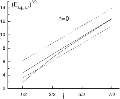
Figure 5: The Regge trajectories for equation (147) with potential (148) (solid line) and for Salpeter equation (151) (dashed line). The lower and the upper line correspond to $l=j-\frac{1}{2}$ and $l=j+\frac{1}{2}$, respectively.

The quasiclassical spectrum of equation (151) demonstrates a linear dependence of $E^{3/2}$ ($E^{(\alpha+1)/\alpha}$ with $\alpha=2$) on the angular momentum $l$, so that, for a given radial quantum number $n$, equation (151) produces two parallel trajectories $E^{3/2}(j)$ with $l=j\pm\frac{1}{2}$. Similar trajectories for equation (147) with potential (148) have a comparable level splitting for small $j$’s which, however, decreases fast with the growth of the angular momentum $l$.

This calculation explicitly demonstrates the phenomenon of the effective restoration of chiral symmetry in the spectrum of highly excited mesons in the Generalised Nambu–Jona-Lasinio model. As one can see by just comparing potentials (150) and (153),

$$E-E^{\prime}\propto\langle\sin\varphi_{p}\rangle,$$ (154)

where $E$ and $E^{\prime}$ are the energies of the opposite-parity states, and averaging over the radial wave function is assumed on the r.h.s.

5.4 Pion decoupling from excited mesons

One of specific predictions for highly excited hadrons with effectively restored chiral symmetry is the decoupling of the chiral pion from them which manifests itself through the decrease of the corresponding coupling constant with the increase of the hadron excitation number [8, 87, 88, 89, 90]. This behaviour of the coupling can be readily established with the help of the Goldberger–Treiman relation for the transitions $n\to n^{\prime}+\pi$, where $n$ and $n^{\prime}$ are the chiral partners, that is, the opposite-parity hadronic states which become degenerate in mass if chiral symmetry is restored in the spectrum.

Let us stick to the BCS approximation first and show that the pion coupling to excited hadrons is defined by the effective mass of the dressed quark. To this end, we consider the axial-vector current (for simplicity, we consider the single-flavour case and the chiral anomaly is omitted),

$$J_{\mu}^{5}(x)=\bar{q}(x)\gamma_{\mu}\gamma_{5}q(x),$$ (155)

which, due to the hypothesis of the Partial Conservation of the Axial-vector Current (PCAC), is related to the wave function of the chiral pion $\phi_{\pi}$,

$$J_{\mu}^{5}(x)=f_{\pi}\partial_{\mu}\phi_{\pi}(x).$$ (156)

Then, with the help of equation (156), it is easy to average the divergence of this current, $\partial_{\mu}J_{\mu}^{5}$, between the states of the dressed quarks,

$$\langle q(p)|\partial_{\mu}J_{\mu}^{5}(x)|q(p^{\prime})\rangle=f_{\pi}m_{\pi}^{2}\langle q(p)|\phi_{\pi}(x)|q(p^{\prime})\rangle\propto f_{\pi}g_{\pi}(q^{2})(\bar{u}_{p}\gamma_{5}u_{p^{\prime}}),\quad q=p-p^{\prime},$$ (157)

where we have introduced the pion-quark-quark form factor $g_{\pi}(q^{2})$.

On the other hand, if chiral symmetry is spontaneously broken and the quark wave functions obey the effective Dirac equation with the dynamically generated mass $m_{q}^{\rm eff}$ then, with the help of equation (155), it is easy to arrive at

$$\langle q(p)|\partial_{\mu}J_{\mu}^{5}(x)|q(p^{\prime})\rangle\propto m_{q}^{\rm eff}(\bar{u}_{p}\gamma_{5}u_{p^{\prime}}).$$ (158)

Equating the r.h.s.’s of equations (157) and (158) one finds that

$$f_{\pi}g_{\pi}=m_{q}^{\rm eff},\quad g_{\pi}\equiv g_{\pi}(m_{\pi}^{2}),$$ (159)

where, for simplicity, all numerical coefficients are absorbed into the definition of the coupling constant $g_{\pi}$. From equation (11) one can see that the effective mass of the quark is described by the quantity $A_{p}$. Then, with the help of relation (159), it is straightforward to find finally that [91]

$$f_{\pi}g_{\pi}(p)\simeq A_{p}.$$ (160)

Beyond the BCS level, the Goldberger–Treiman relation connects the pion coupling constant to an excited hadron with the mass splitting between the two hadronic chiral partners. For definiteness, let us consider the transition ${\bar{D}}(J^{P}=0^{+})\to{\bar{D}}^{\prime}(J^{P}=0^{-})\pi$, where the quark contents of the $\bar{D}^{(\prime)}$ meson is $\bar{c}q$ with the light quark $q=u,d$.

From PCAC condition (156), generalised to the isospin group $SU(2)$, one has

$$\langle 0|J_{\mu}^{5a}(0)|\pi^{b}({\bm{q}})\rangle=if_{\pi}q_{\mu}\delta^{ab},$$ (161)

so that for the transition matrix element $\langle n^{\prime}|J_{\mu}^{5a}|n\rangle$ ($n^{(\prime)}=\bar{D}^{(\prime)}$) it is easy to find

$$\langle n^{\prime}|J_{\mu}^{5a}|n\rangle=\langle n^{\prime}|J_{\mu}^{5a}|n\rangle_{\mbox{nonpion}}-\frac{2Mq_{\mu}f_{\pi}g_{nn^{\prime}\pi}}{q^{2}-M_{\pi}^{2}+i0}D^{\prime{\dagger}}\tau^{a}D,$$ (162)

where we introduced the pion coupling constant $g_{nn^{\prime}\pi}$ and the isospin doublets $D$ and $D^{\prime}$.

On the other hand, it is easy to establish the most general form of the l.h.s. of equation (162) compatible with Lorentz invariance,

$$\langle n^{\prime}|J_{\mu}^{5a}|n\rangle=\left[(P_{\mu}+P^{\prime}_{\mu})G_{A}(q^{2})-(P_{\mu}-P^{\prime}_{\mu})G_{S}(q^{2})\right]D^{\prime{\dagger}}\left(\frac{\tau^{a}}{2}\right)D,$$ (163)

where $P_{\mu}$ and $P_{\mu}^{\prime}$ are the momenta of the initial and final $D$ meson, respectively, and $q_{\mu}=P_{\mu}-P^{\prime}_{\mu}$. Then, in the leading order in the heavy-quark mass, conservation of the axial-vector current leads to the condition

$$2M(M-M^{\prime})G_{A}-q^{2}G_{S}=0.$$ (164)

In the meantime, from relation (162) one can see that, in the limit $q^{2}\to 0$, one has $G_{A}(0)\equiv G_{A}\neq 0$ if $G_{S}$ is identifies with the pion pole, that is,

$$\lim_{q^{2}\to 0}G_{S}(q^{2})\to\frac{4Mf_{\pi}g_{nn^{\prime}\pi}}{q^{2}}.$$ (165)

The resulting equation,

$$\frac{1}{2}(M-M^{\prime})G_{A}=f_{\pi}g_{nn^{\prime}\pi},$$ (166)

is nothing but the sought Goldberger–Treiman relation for the heavy-light mesons. This relation implies that, as the excitation of the $D$ grows and, therefore, as its degeneracy with its chiral partner $D^{\prime}$ becomes more manifest, the pion decouples from this meson.

Figure 6: The $n\to n^{\prime}+\pi$ transition amplitude.

Let us now derive relations (160) and (166) microscopically. Consider the pion emission process by the hadron $n$ (here hadrons $n$ and $n^{\prime}$ are mesons; the case of the baryons is studied in the next chapter), $n\to n^{\prime}+\pi$. The corresponding diagrams are depicted in Fig. 6 and the matrix element reads

$$\begin{array}[]{c}\displaystyle M(n\to n^{\prime}+\pi)=\int\frac{d^{4}k}{(2\pi)^{4}}\textrm{Tr}\left[\chi_{n}({\bm{k}},{\bm{P}})S(k-P)\bar{\chi}_{n^{\prime}}({\bm{k}}-{\bm{P}},{\bm{P}}^{\prime})S(k-q)\bar{\chi}_{\pi}({\bm{k}},{\bm{q}})S(k)\right]\\[8.53581pt] \displaystyle+\int\frac{d^{4}k}{(2\pi)^{4}}\textrm{Tr}\left[\chi_{n}({\bm{k}},{\bm{P}})S(k-P)\bar{\chi}_{\pi}({\bm{k}},{\bm{q}})S(k-q)\bar{\chi}_{n^{\prime}}({\bm{k}}-{\bm{P}},{\bm{P}}^{\prime})S(k)\right],\end{array}$$ (167)

where $q=P-P^{\prime}$ and each hadronic vertex contains the amplitude $\chi$ ($\bar{\chi}$ for the outgoing meson) which obeys Bethe-Salpeter equation (33). Thus, the pion emission vertex is given by the overlap of the three vertex functions. The maximal overlap is achieved if the wave functions of all three mesons are localised in the same region in momentum. As it happens, the pion wave function (44) is localised at small relative momenta between the quark and the antiquark and it decreases fast with increased momentum. The wave functions of the mesons $n$ and $n^{\prime}$ are localised at approximately the same momenta which grow with the excitation number. This implies that the overlap of the vertex functions decreases with the growth of the excitation of the meson $n$ and so does the pion coupling constant.

In order to describe this effect quantitatively we write the matrix vertex $\chi({\bm{p}},{\bm{P}})$ through the matrix wave function defined in equation (44),

$$\chi({\bm{p}},{\bm{P}})=\int\frac{d^{3}k}{(2\pi)^{3}}V({\bm{p}}-{\bm{k}})\gamma_{0}\tilde{\phi}({\bm{k}},{\bm{P}})\gamma_{0}.$$ (168)

The matrix vertex for the incoming meson is simply related to the vertex for the outgoing meson,

$$\bar{\chi}({\bm{p}},{\bm{P}})=\gamma_{0}\chi^{\dagger}({\bm{p}},{\bm{P}})\gamma_{0}.$$ (169)

The explicit form of the matrix wave function $\tilde{\phi}_{\pi}$ for the pion at rest (${\bm{P}}_{\pi}\equiv{\bm{q}}\to 0$) is given by equation (59) while the components $\varphi_{\pi}^{\pm}$ are quoted in equation (55). Then it is easy to find for the pion emission vertex $\bar{\chi}_{\pi}({\bm{p}},{\bm{q}}=0)\equiv\bar{\chi}_{\pi}({\bm{p}})$ that

$$f_{\pi}\bar{\chi}_{\pi}({\bm{p}})=\sqrt{\frac{2\pi N_{C}}{m_{\pi}}}\gamma_{5}\int\frac{d^{3}k}{(2\pi)^{3}}V({\bm{p}}-{\bm{k}})\sin\varphi_{k}={\rm const}\times\gamma_{5}A_{p},$$ (170)

where definition (11) for the function $A_{p}$ was used. If the pion form factor $g_{\pi}(p)$ is defined with the same constant as in equation (170),

$$\bar{u}_{p}\bar{\chi}_{\pi}({\bm{p}})u_{p}={\rm const}\times g_{\pi}(p)(\bar{u}_{p}\gamma_{5}u_{p}),$$ (171)

then we finally arrive at the Goldberger–Treiman relation in the form

$$f_{\pi}g_{\pi}(p)=A_{p},$$ (172)

that coincides with formula (160), but now this relation is derived rigorously.

It is important to emphasise an essential difference between equations (172) and (159), with the latter taken naïvely. Indeed, naïvely, one could conclude that the r.h.s. of equation (159) contains the quantity which depends only on the momentum transfer in the pion emission vertex, that is, on the pion momentum ${\bm{q}}=0$. Then $m_{q}^{\rm eff}$ has to be treated as a constant, independent of the excitation number of the hadron which emits the pion. The same would be true for the pion coupling $g_{\pi}$. However, the microscopic treatment performed above demonstrates that the pion emission vertex is a function of two variables: the pion momentum and the loop momentum floating through the pion emission vertex. The latter quantity also plays the role of the momentum of the quark interacting with the pion. Therefore, even in the limit ${\bm{q}}=0$, the r.h.s of equation (172) is a decreasing function of the momentum rather than a constant. It is easy to estimate its decrease rate. Indeed, in the chiral limit, $A_{p}=E_{p}\sin\varphi_{p}$, while, for large momenta, $E_{p}\approx p$ with the chiral angle behaving as $\varphi_{p}\propto 1/p^{4+\alpha}$, where $\alpha$ is the parameter of the power-like potential (see equation (25)). Thus,

$$g_{\pi}(p)\mathop{\sim}_{p\to\infty}\frac{1}{p^{\alpha+3}}.$$ (173)

Figure 7: Dependence of the ratio $g_{\pi}(p)/g_{\pi}(0)$ on the momentum evaluated for the Harmonic Oscillator potential. For definiteness, the parameter $K_{0}$ is fixed as in equation (143).

The result of the numerical calculation of the ratio $g_{\pi}(p)/g_{\pi}(0)$ for the Harmonic Oscillator potential ($\alpha=2$), given in Fig. 7, shows that, indeed, the pion coupling decreases with the quark momentum growth.

To finalise this chapter, let us derive microscopically Goldberger–Treiman relation (166) for the pion emission by a heavy-light meson [92].

First, we proceed from the nonrelativistic normalisation (57) for the pion wave functions (55) to the relativistic one, so that we define the wave functions

$$X_{p}=\frac{\sqrt{N_{C}}}{f_{\pi}}\left[\sin\varphi_{p}+M_{\pi}\Delta_{p}\right],\quad Y_{p}=\frac{\sqrt{N_{C}}}{f_{\pi}}\left[\sin\varphi_{p}-M_{\pi}\Delta_{p}\right].$$ (174)

Then one can find that

$$\int\frac{d^{3}p}{(2\pi)^{3}}\Bigl{(}X_{p}^{2}-Y_{p}^{2}\Bigr{)}=2M_{\pi},$$ (175)

and the pionic field with the isospin projection $a$ in its rest frame can be written in the form

$$|\pi^{a}\rangle=\frac{1}{\sqrt{N_{C}}}\sum_{\alpha=1}^{N_{C}}\sum_{s_{1},s_{2}=\uparrow,\downarrow}(\sigma_{2})_{s_{1}s_{2}}\sum_{i_{1},i_{2}=\pm 1/2}\left(\frac{\tau^{a}}{2}\right)^{i_{1}i_{2}}\int\frac{d^{3}p}{(2\pi)^{3}}\left[b_{\alpha,s_{1}i_{1}}^{\dagger}({\bm{p}})d_{s_{2}i_{2}}^{\alpha{\dagger}}(-{\bm{p}})X_{p}+\right.$$

(176)

$$\left.\hskip 199.16928pt+d_{s_{2}i_{2}}^{\alpha}(-{\bm{p}})b_{\alpha,s_{1}i_{1}}({\bm{p}})Y_{p}\right]|0\rangle,$$

where $|0\rangle$ is the BCS vacuum.

The wave functions of the pseudo-scalar and scalar heavy-light mesons which obey equations (113) and (139) can be written in the form

$$\psi({\bm{p}})=\frac{i}{\sqrt{2}}\sigma_{2}\phi_{p},\quad\psi^{\prime}({\bm{p}})=({\bm{\sigma}}\hat{{\bm{p}}})\psi({\bm{p}})=\frac{i}{\sqrt{2}}({\bm{\sigma}}\hat{{\bm{p}}})\sigma_{2}\phi^{\prime}_{p}$$ (177)

and normalised by the relativistic conditions,

$$\textrm{Tr}\int\frac{d^{3}p}{(2\pi)^{3}}|\psi({\bm{p}})|^{2}=\int\frac{d^{3}p}{(2\pi)^{3}}\phi_{p}^{2}=2M,\quad\textrm{Tr}\int\frac{d^{3}p}{(2\pi)^{3}}|\psi^{\prime}({\bm{p}})|^{2}=\int\frac{d^{3}p}{(2\pi)^{3}}\phi_{p}^{\prime 2}=2M^{\prime},$$ (178)

where the trace is taken in the spin indices. Besides, in the above normalisation conditions one can set $M=M^{\prime}$.

The pion coupling constant $g_{nn^{\prime}\pi}$ is defined through the relation

$$\langle{\bar{D}}^{\prime}\pi^{a}|V|{\bar{D}}\rangle=2Mig_{nn^{\prime}\pi}(D^{{}^{\prime}{\dagger}}\tau^{a}D)(2\pi)^{3}\delta^{(3)}({\bm{P}}^{\prime}+{\bm{q}}-{\bm{P}}),$$ (179)

where $V$ is the interaction responsible for the pion emission. In what follows, we shall evaluate the matrix element on the l.h.s of equation (179) in the framework of the Generalised Nambu–Jona-Lasinio model.

Figure 8: The diagrams contributing to the matrix element $\langle{\bar{D}}^{\prime}\pi|V|{\bar{D}}\rangle$.

In Fig. 8 we draw the four diagrams contributing to the matrix element $\langle{\bar{D}}^{\prime}\pi|V|{\bar{D}}\rangle$ for which we can write then

$$\langle{\bar{D}}^{\prime}\pi^{a}|V|{\bar{D}}\rangle=2M\left[A^{a}_{X}+B^{a}_{Y}+C^{a}_{X}+D^{a}_{Y}\right](2\pi)^{3}\delta^{(3)}({\bf P}^{\prime}+{\bm{q}}-{\bf P}),$$ (180)

where the contributions $A^{a}_{X}$ and $B^{a}_{Y}$ cancel against each other while the amplitudes $C^{a}_{X}$ and $D^{a}_{Y}$ take the form [92]

$$C^{a}_{X} = \frac{(D^{\prime}\tau^{a}D)}{4M\sqrt{N_{C}}}\int\frac{d^{3}k}{(2\pi)^{3}}\frac{d^{3}p}{(2\pi)^{3}}\phi^{\prime}_{p}V({\bm{p}}-{\bm{k}})X_{k}\phi_{k}[S_{p}C_{k}-(\hat{{\bm{p}}}\hat{{\bm{k}}})C_{p}S_{k}],$$

$$D^{a}_{Y} = \frac{(D^{\prime}\tau^{a}D)}{4M\sqrt{N_{C}}}\int\frac{d^{3}k}{(2\pi)^{3}}\frac{d^{3}p}{(2\pi)^{3}}\phi^{\prime}_{p}V({\bm{p}}-{\bm{k}})Y_{p}\phi_{k}[S_{p}C_{k}-(\hat{{\bm{p}}}\hat{{\bm{k}}})C_{p}S_{k}],$$

where $C_{p}$ and $S_{p}$ are defined in (40) and their products stem from the vertices shown in the diagrams as black dots and given by various products of the dressed quark bispinors (6).

For instance, in the amplitude $A_{X}^{a}$ (see Fig. 8) one has the following combination:

$$u^{\dagger}({\bm{p}})u({\bm{k}})=C_{p}C_{k}+({\bm{\sigma}}\cdot\hat{{\bm{p}}})({\bm{\sigma}}\cdot\hat{{\bm{k}}})S_{p}S_{k}.$$ (182)

Now, taking relations (179), (180), and (LABEL:CD) together and using the explicit form of the pion wave functions (174), it is easy to find for the coupling constant $g_{nn^{\prime}\pi}$ in the leading order in $M_{\pi}$ [92],

$$f_{\pi}g_{nn^{\prime}\pi}=\frac{1}{2M}\int\frac{d^{3}k}{(2\pi)^{3}}\frac{d^{3}p}{(2\pi)^{3}}\phi_{p}^{\prime}V({\bm{p}}-{\bm{k}})\phi_{k}(\sin\varphi_{p}+\sin\varphi_{k})[S_{p}C_{k}-(\hat{{\bm{p}}}\hat{{\bm{k}}})C_{p}S_{k}].$$ (183)

The nonpion contribution to the off-diagonal axial charge $G_{A}$ can be evaluated with the help of the explicit expression for the temporal component of the axial-vector current and it takes the form [92]

$$G_{A}=\frac{1}{2M}\int\frac{d^{3}k}{(2\pi)^{3}}\phi^{\prime}_{k}\phi_{k}\cos\varphi_{k}.$$ (184)

To proceed, we multiply equation (113) for the wave function $\psi({\bm{p}})$ by $\psi^{\prime}({\bm{p}})\cos\varphi_{p}$, take trace in the spinor indices, and integrate both sides of the resulting equation in the momentum $d^{3}p/(2\pi)^{3}$. Then we repeat the above procedures for equation (139) for the wave function $\psi^{\prime}({\bm{p}})$, now multiplied by $\psi({\bm{p}})\cos\varphi_{p}$. Subtracting one resulting equation from the other, we arrive at the relation

$$\frac{1}{2}(E-E^{\prime})G_{A}=\frac{1}{2M}\int\frac{d^{3}k}{(2\pi)^{3}}\frac{d^{3}p}{(2\pi)^{3}}\phi_{p}^{\prime}V({\bm{p}}-{\bm{k}})\phi_{k}[\cos\varphi_{p}(C_{p}C_{k}+(\hat{{\bm{p}}}\hat{{\bm{k}}})S_{p}S_{k})-$$

(185)

$$-\cos\varphi_{k}((\hat{{\bm{p}}}\hat{{\bm{k}}})C_{p}C_{k}+S_{p}S_{k})].$$

After simple trigonometric transformations the r.h.s. of the last equation reduces to that of relation (183). Therefore, equating the l.h.s.’s of equations (183) and (185) and proceeding from the energies $E$ and $E^{\prime}$ to the corresponding masses (that is, adding the mass of the heavy antiquark), we finally arrive at Goldberger–Treiman relation (166).

Two comments are in order here. On the one hand, it is easy to see that the role played by the $Y$ ($\varphi_{\pi}^{-}$) component of the pion wave function in the derivation of relation (166) is as important as the role of the component $X$ ($\varphi_{\pi}^{+}$). This emphasises once more the Goldstone nature of the chiral pion which as a matter of principle cannot be described in naïve (constituent) quark models.

On the other hand, it follows from equation (184), from the properties of the chiral angle, and from normalisation condition (177) that for excited mesons the axial charge approaches unity, $G_{A}\mathop{\to}\limits_{n\to\infty}1$. Therefore, as it was stated above, for highly excited mesons, the pion coupling constant decreases,

$$g_{nn^{\prime}\pi}=\frac{G_{A}\Delta M_{\pm}}{2f_{\pi}}\propto\Delta M_{\pm}\mathop{\to}\limits_{n\to\infty}0,$$ (186)

and that implies that the Goldstone boson decouples from the spectrum of excited heavy-light quarkonia.

5.5 Effective chiral symmetry restoration in the spectrum of excited baryons

In the previous chapters we studied in detail the problem of the effective restoration of chiral symmetry in the spectrum of highly excited hadrons and the related question of the chiral pion (Goldstone boson) decoupling from the spectrum of highly excited mesons. A similar situation takes place in the spectrum of excited baryons. We start from a general symmetry-based discussion.

Consider a chiral doublet $B$ built from the effective baryonic fields of the opposite parity $B_{+}$ and $B_{-}$ [54],

$$B=\genfrac{(}{)}{0.0pt}{0}{B_{+}}{B_{-}}.$$ (187)

The states $B_{+}$ and $B_{-}$ are mixed by the axial transformation,

$$B\to\exp\left(i\frac{\theta^{a}_{A}\tau^{a}}{2}\sigma_{1}\right)B,$$ (188)

where $\sigma_{1}$ is the Pauli matrix in the space of the doublet $B$. It is easy to establish the form of the Lagrangian invariant with respect to the above transformation (for the alternative forms of this Lagrangian see papers [93, 94]),

$$\mathcal{L}_{0}=i\bar{B}\gamma^{\mu}\partial_{\mu}B-m_{0}\bar{B}B=i\bar{B}_{+}\gamma^{\mu}\partial_{\mu}B_{+}+i\bar{B}_{-}\gamma^{\mu}\partial_{\mu}B_{-}-m_{0}\bar{B}_{+}B_{+}-m_{0}\bar{B}_{-}B_{-}.$$ (189)

An important property of the given Lagrangian is the presence of a nonvanishing chirally invariant mass $m_{0}$, the same for the opposite-parity fields. This implies the Wigner-Weyl realisation of chiral symmetry with massive fermions. Chiral doublets are inevitable in this scenario. Therefore, in the spectrum of baryons, in addition to the “standard” scenario when the fermion mass emerges as a result of the spontaneous breaking of chiral symmetry (Nambu–Goldstone realisation), an alternative realisation is possible which is consistent with chiral doublets. It is straightforward to build the Noether current which corresponds to symmetry (188) of Lagrangian (189),

$$j^{a}_{5\mu}=\bar{B}_{+}\gamma_{\mu}\frac{\tau^{a}}{2}B_{-}+\bar{B}_{-}\gamma_{\mu}\frac{\tau^{a}}{2}B_{+},$$ (190)

which does not contain diagonal terms of the form either $\bar{B}_{+}\gamma_{\mu}\gamma_{5}\frac{\tau^{a}}{2}B_{+}$ or $\bar{B}_{-}\gamma_{\mu}\gamma_{5}\frac{\tau^{a}}{2}B_{-}$. Therefore, the diagonal axial charges of the baryons $B_{+}$ and $B_{-}$ which form the chiral doublet vanish while the off-diagonal axial charges related to the transitions between the opposite-parity states equal to unity [54],

$$G_{A}^{+}=G_{A}^{-}=0,\quad G_{A}^{+-}=G_{A}^{-+}=1.$$ (191)

It has to be noticed that the axial charge of the standard Dirac fermion equals to 1.

It is easy to trace the consequences of property (191). Firstly, the diagonal pion couplings to baryons must vanish in unison with the diagonal axial charges of the baryons, that is, $g_{\pi B_{\pm}B_{\pm}}=\frac{G_{A}^{\pm}m_{\pm}}{f_{\pi}}=0$.

Below, we derive the formulae for the off-diagonal constant $g_{\pi B_{+}B_{-}}$. To this end, consider the matrix element of the axial-vector current between two arbitrary opposite-parity baryonic states, $1/2^{+}$ and $1/2^{-}$,

$$\langle B_{-}(p_{f})|j^{a}_{5\mu}|B_{+}(p_{i})\rangle=\bar{u}(p_{f})\left[\gamma_{\mu}H_{1}(q^{2})+\sigma_{\mu\nu}q^{\nu}H_{2}(q^{2})+q_{\mu}H_{3}(q^{2})\right]\frac{\tau^{a}}{2}u(p_{i}),$$ (192)

where $p_{i}$ and $p_{f}$ are the initial-state and the final-state momenta, respectively, ($q=p_{f}-p_{i}$) and we introduced the form factors $H_{1}$, $H_{2}$, and $H_{3}$. Then, for the matrix element of the divergence of the axial-vector current we arrive at

$$\langle B_{-}(p_{f})|\partial^{\mu}j^{a}_{5\mu}|B_{+}(p_{i})\rangle=i\left[(m_{+}-m_{-})H_{1}(q^{2})+q^{2}H_{3}(q^{2})\right]\bar{u}(p_{f})\frac{\tau^{a}}{2}u(p_{i}).$$ (193)

Once the l.h.s. of equation (193) vanishes in the chiral limit due to the PCAC condition, then, in the limit $q\to 0$, the form factors must obey the following condition:

$$(m_{+}-m_{-})H_{1}(0)+\lim_{q\to 0}q^{2}H_{3}(q^{2})=0,$$ (194)

which can be easily recognised as the Goldberger–Treiman relation,

$$g_{\pi B_{+}B_{-}}=\frac{G_{A}^{+-}(m_{+}-m_{-})}{2f_{\pi}},\quad G_{A}^{+-}=H_{1}(0).$$ (195)

Indeed, PCAC requires that the contribution of the term proportional to $H_{1}$ is compensated by the term proportional to $H_{3}$, and the latter has to develop a pole at $q^{2}\to 0$ which is identified naturally with the Goldstone pole. Thus, if the states $B^{\pm}$ belong to the same chiral doublet then they become degenerate in the mass that ensures that $g_{\pi B_{+}B_{-}}=0$, and this condition, being a consequence of PCAC, is independent of the particular degeneracy mechanism for the states $B^{\pm}$.

Similarly to mesons, the general symmetry-based arguments given above possess a particular microscopic realisation in the framework of the Generalised Nambu–Jona-Lasinio model. However, it is important to make a comment on the baryonic states in this model. In spite of the fact that the model is considered in the formal limit $N_{C}\to\infty$, properties of the baryons can be studied qualitatively (in many cases also quantitatively) if $N_{C}=3$ is substituted. Then the baryon can be built by acting the three dressed-quark operators on the BCS vacuum and contracting the result with the relevant wave function,

$$\Psi_{B}=\Psi_{\rm colour}\otimes\Psi_{\rm flavour}\otimes\Psi_{\rm spin}\otimes\Psi_{\rm space},\quad\Psi_{\rm colour}=\frac{1}{3!}\varepsilon_{\alpha\beta\gamma}q^{\alpha}q^{\beta}q^{\gamma},$$ (196)

where $\varepsilon_{\alpha\beta\gamma}$ is the antisymmetric Levi-Civita tensor. Baryons do not bring any new effects to the model and, even more, the Dyson equations for baryons turn out to be much simpler than the similar equations for mesons. The simplification comes from the fact that for baryons the positive-energy component of the amplitude does not couple to the negative-energy component, for such transitions would imply the existence of the states with open colour (see Fig. 9).

Figure 9: Diagram A: a typical colour-allowed (singlet — singlet, $0_{c}\rightarrow 0_{c}$) transition between the positive-energy and negative-energy amplitudes for the $q\bar{q}$ pair. Diagram B: a similar transition is forbidden in the baryon since it results in the state with an open colour ($3_{c}$). Diagram C: a typical colour-allowed diagram contributing to the Dyson equation for the baryon in the ladder approximation.

Since, by construction, the colour wave function of the baryon is antisymmetric with respect to the permutation of the quarks, then it is sufficient to study only symmetric combinations $\Psi_{\rm flavour}\otimes\Psi_{\rm spin}\otimes\Psi_{\rm space}$, so that in the generic case the spatial wave function $\Psi_{\rm space}^{{\cal Y}}({\bm{\rho}},{\bm{\lambda})}$ (here $\bm{\rho}$ and $\bm{\lambda}$ are the standard Jacobi coordinates) should contain all possible permutations ${\cal Y}$: antisymmetric (${\cal A}$), symmetric (${\cal S}$), and mixed $F$ (${\cal D}_{F}$) or $D$ (${\cal D}_{D}$). So far, all considerations were quite general while below in this chapter a particular form of some baryonic wave functions will be quoted and used to calculate the axial charges of these baryons.

Consider the operator of the axial charge,

$$Q_{5}^{a}=\int d^{3}x\;\bar{\psi}_{i}\gamma_{0}\gamma_{5}\left(\frac{\tau^{a}}{2}\right)^{ij}\psi_{j},$$ (197)

and evaluate it for the dressed quarks using equations (5) and (6). The result reads [95]

$$Q_{5}^{a}=\sum_{i,j}\sum_{\alpha=1}^{N_{C}}\sum_{s,s^{\prime}=\uparrow,\downarrow}\left(\frac{\tau^{a}}{2}\right)^{ij}\int\frac{d^{3}p}{(2\pi)^{3}}\Bigl{[}\cos\varphi_{p}({\bm{\sigma}}\hat{\bm{p}})_{ss^{\prime}}\Bigl{(}b_{i\alpha s}^{\dagger}({\bm{p}})b_{js^{\prime}}^{\alpha}(-{\bm{p}})+d_{js}^{\alpha\dagger}(-{\bm{p}})d_{i\alpha s^{\prime}}({\bm{p}})\Bigr{)}$$

(198)

$$\hskip 142.26378pt+\sin\varphi_{p}(i\sigma_{2})_{ss^{\prime}}\Bigl{(}b_{i\alpha s}^{\dagger}({\bm{p}})d^{\alpha\dagger}_{js^{\prime}}(-{\bm{p}})+d_{i\alpha s}({\bm{p}})b_{js^{\prime}}^{\alpha}(-{\bm{p}})\Bigr{)}\Bigr{]},$$

where the two contributions in the square brackets have different physical interpretation. The first term is diagonal in the quark creation and annihilation operators (nonanomalous term) and because it contains the operator $({\bm{\sigma}}\hat{{\bm{p}}})$ it is responsible for the transition from the baryonic state with a given parity to the baryonic state with the opposite parity, that is, to the chiral partner. The second term in equation (198) has the content of a Bogoliubov anomalous term. Since the axial current is a component of the conserved Noether current and, therefore, it commutes with the Hamiltonian, $[Q_{5}^{a},H]=0$, then the state $Q_{5}^{a}|0\rangle=|\pi^{a}\rangle$ is degenerate with the vacuum and it is the Goldstone boson, that is, it is nothing but the chiral pion. Indeed, the quantity $\sin\varphi_{p}(i\sigma_{2})$ is the wave function of the pion in its rest frame — see equations (55) and (71).

Consider the diagonal part of the axial charge operator of a baryon defined as the sum of operators (198) over all quarks in the baryon,

$${\cal Q}_{5}\equiv{\cal Q}_{5}^{3}=\sum_{n=1}^{3}Q_{5n}^{3}.$$ (199)

From the above consideration, it is easy to see that the result of such an operator acting on the baryonic state can be schematically presented in the form

$${\cal Q}_{5}|B\rangle=|B^{\prime}\rangle+|B\pi\rangle,$$ (200)

where the first term on the r.h.s. describes the chiral partner of the state $|B\rangle$ and the second term contains the neutral pion. The relative weight of the above two terms is defined by the chiral angle $\varphi_{p}$. In particular, in case of the maximal symmetry breaking $\varphi_{p}=\pi/2$ and, therefore, only the second term survives on the r.h.s. of equation (200). In the opposite limit of unbroken chiral symmetry $\varphi_{p}=0$, so that only the first term survives. In this case it is easy to arrive at the following (obvious) properties of the operator ${\cal Q}_{5}$:

$${\cal Q}_{5}^{\dagger}={\cal Q}_{5},\quad\langle B_{2}|{\cal Q}_{5}^{2}|B_{1}\rangle\propto\langle B_{2}|B_{1}\rangle=\delta_{B_{1}B_{2}}.$$ (201)

Therefore,

$${\cal Q}_{5}|B^{\pm}\rangle=G_{A}^{\pm\raisebox{-1.42262pt}{\scriptsize$\mp$}}|B^{\mp}\rangle,$$ (202)

where $B^{\pm}$ stand for the opposite-parity baryons and $G_{A}^{\pm\raisebox{-1.42262pt}{\scriptsize$\mp$}}$ stand for the axial charges. Then, for the baryon spectrum in the limit of the exact chiral symmetry restoration the following relations between various axial charges hold true:

$$G_{A}^{+-}=G_{A}^{-+}=1,\quad G_{A}^{++}\equiv G_{A}^{+}=0,\quad G_{A}^{--}\equiv G_{A}^{-}=0,$$ (203)

which are approached asymptotically with the growth of the excitation number of the baryon. Once, as was mentioned above, the axial charge operator commutes with the Hamiltonian, then the states $|B^{+}\rangle$ and $|B^{-}\rangle$ should become degenerate in this limit.

5.6 Axial charges of baryons in the nonrelativistic quark model

In the previous chapter, the effective restoration of chiral symmetry in the spectrum of excited baryons was described in detail in the framework of the microscopical framework provided by the Generalised Nambu–Jona-Lasinio model. In particular, predictions were made for the axial charges of baryons. For comparison, let us evaluate the axial charges of some baryons in a different approach. In particular, a popular alternative approach to baryons is provided by the well-known nonrelativistic $SU(6)$ quark model which includes the $SU(3)$ isospin and $SU(2)$ spin group and which is quite successful in describing the ground states of baryons [96, 97]. All ground-state baryons with the quantum numbers $1/2^{+}$ and $3/2^{+}$, which form the octet and the decuplet, respectively, of the isospin $SU(3)$ group enter the 56-plet of the group $SU(6)$. Then, for example, magnetic moments of baryons (in fact, their ratios) are reproduced in the $SU(6)$ model with accuracy about 10-15%. One of the most well-known predictions of this model, the nucleon axial charge $G_{A}=5/3$, coincides with the experimental value $G_{A}=1.26$ quite well, the discrepancy is caused by the neglected relativistic effects, by the pionic cloud, by the effects of the $SU(6)$ symmetry breaking because of the different quark masses, and so on.

In the large-$N_{C}$ limit, the ground states in the spectrum of baryons indeed obey the $SU(6)$ algebra [98, 99] that is a consequence of the spontaneous breaking of chiral symmetry which results in the emergence of large constituent quark masses. In order to predict the masses of the excited baryons, the symmetry group $SU(6)$ needs to be supplied with the dynamical assumptions about the structure of the radial and angular excitations of the quarks in the baryons. In the simplest case of the Harmonic Oscillator confining potential the energy of the quarks is fully fixed by the principal quantum number, and the masses of the excited negative-parity states of the nucleon and the $\Delta$ agree well with the predictions of such a $SU(6)\times O(3)$ classification scheme with $N=1$. However, for the positive-parity states, the given scheme meets certain difficulties such as an overestimated splitting with the negative-parity states and, for the Roper resonance, with the wrong ordering of the opposite-parity levels. In the literature, there exist successful attempts to resolve the aforementioned difficulties through a particular symmetry breaking mechanism [100]. However, a systematic mass degeneracy of opposite-parity excited baryons looks quite unnatural in the framework of this quark model and there is no explanation for this phenomenon. In particular, in the $SU(6)\times O(3)$ scheme there are no reasons whatsoever for the axial charges of the baryons to obey formula (203). Meanwhile, once the axial charges of baryons can be evaluated on the lattice (see, for example, papers [97, 101, 102, 103, 104]) then it would be natural to confront the lattice results with the predictions of the quark model $SU(6)\times O(3)$ in which the effective restoration of chiral symmetry is not possible. Then, deviations of the lattice data from the predictions of the quark model can be interpreted as an argument in favour of the chiral symmetry restoration in the spectrum of excited baryons.

In order to evaluate the axial charges of baryons in the nonrelativistic quark model one needs to work out the averages over the baryons’ wave functions of the form

$$G_{A}^{fi}=\langle\Psi_{f}(1,2,3)|\sum_{n=1}^{3}Q^{A}_{n}|\Psi_{i}(1,2,3)\rangle,$$ (204)

where $Q^{A}_{n}$ is the operator of the axial charge of the $n$-th quark which in the leading order is given by the Gamov–Teller formula $\sigma_{3}\tau_{3}$ (here ${\bm{\sigma}}$ and ${\bm{\tau}}$ are the spin and the isospin operators of the Dirac fermion, respectively). This operator admits relativistic corrections (which, however, will not be considered below) of the form

$$\frac{1}{2M}{\bm{\sigma}}({\bm{p}}_{i}+{\bm{p}}_{f})\tau^{a}e^{i\bm{q}\bm{r}},$$ (205)

where ${\bm{q}}={\bm{p}}_{f}-{\bm{p}}_{i}$. In addition, the operator of the axial charge of a nonrelativistic quark in the leading order also contains a dependence on the spatial coordinate in form of the exponent $\exp{[i{\bm{q}}{\bm{r}}]}$. However, evaluation of both the diagonal and off-diagonal axial charges amounts to taking the limit ${\bm{q}}\to 0$ [105]. Then, in the leading order, the operator of the axial charge does not depend on the coordinate and, therefore, matrix element (204) is nonzero only if the spatial wave functions of the initial and the final baryons coincide. This prediction of the $SU(6)\times O(3)$ scheme appears to be at odds with the predictions of the chiral symmetry restoration in the spectrum and, in particular, with its microscopic realisation in the framework of the Generalised Nambu–Jona-Lasinio model — see equation (203).

Evaluation of the diagonal matrix elements (204) requires one to know the wave functions of the baryons in the $SU(6)\times O(3)$ scheme which are well-known in the literature and are quoted in Table 3. Each wave function is characterised by several quantum numbers. First, there is the multiplet of the spin-flavour group $SU(6)$ to which the given state belongs and which is encoded in the Young symbol $[f]_{FS}$. In each such multiplet the baryon’s wave function possesses a particular symmetry in the flavour space (symbol $[f]_{F}$ with $f=3,21,111$) and a particular spin symmetry (symbol $[f]_{S}$ with $f=3,21$ for $S=3/2$ and $S=1/2$, respectively). Finally, the spatial part of the wave function is fixed by the angular momentum $L$ and by the permutation symmetry $[f]_{X}$ which is fixed by the Pauli principle as $[f]_{X}=[f]_{FS}$. For a particular basis used, additional quantum numbers may arise like the principal quantum number $N$ in the Harmonic Oscillator basis or the spatial symmetry of the angular wave function $(\lambda\mu)$.

$N(\lambda\mu)L[f]_{X}[f]_{FS}[f]_{F}[f]_{S}$	$J^{P}$,
$0(00)0[3]_{X}[3]_{FS}[21]_{F}[21]_{S}$	$\frac{1}{2}^{+},N$
$2(20)0[3]_{X}[3]_{FS}[21]_{F}[21]_{S}$	$\frac{1}{2}^{+},N(1440)$
$1(10)1[21]_{X}[21]_{FS}[21]_{F}[21]_{S}$	$\frac{1}{2}^{-},N(1535)\quad\frac{3}{2}^{-},N(1520)$
$1(10)1[21]_{X}[21]_{FS}[21]_{F}[3]_{S}$	$\frac{1}{2}^{-},N(1650)\quad\frac{3}{2}^{-},N(1700)\quad\frac{5}{2}^{-},N(1675)$
$2(20)2[3]_{X}[3]_{FS}[21]_{F}[21]_{S}$	$\frac{3}{2}^{+},N(1720)\quad\frac{5}{2}^{+},N(1680)$
$2(20)0[21]_{X}[21]_{FS}[21]_{F}[21]_{S}$	$\frac{1}{2}^{+},N(1710)$

Table 3: Wave functions of some nucleons in the mass region below 2 GeV in the $SU(6)$ scheme (see, for example, reference [100]).

The diagonal axial charges of some baryons evaluated with the help of the wave functions quoted in Table 3 are given in Table 4 (the details of the calculations can be found in paper [105]). The charges found allow one to compare the predictions of the $SU(6)$ model with the predictions of the chiral restoration model. In particular, the states $N(1440)$ and $N(1535)$ form a chiral doublet and, therefore, according to the model of chiral restoration, their axial charges should be small. From Table 4 one can see that the $SU(6)$ model also predicts a small axial charge for the $N(1535)$, however, for the state $N(1440)$ the prediction of this model is rather large — larger than unity. A similar situation takes place for another pair of chiral partners — for $N(1710)$ and $N(1650)$: the $SU(6)$ model predicts rather large values of both axial charges. Other examples of model calculations of the axial charges of excited baryons can be found in papers [106, 107, 108, 109, 110].

Baryon	$N(1440)$	$N(1710)$	$N(1535)$	$N(1650)$
$J^{P}$	$1/2^{+}$	$1/2^{+}$	$1/2^{-}$	$1/2^{-}$
$G_{A}$	$5/3$	$1/3$	$-1/9$	$5/9$

Table 4: Diagonal axial charges of baryons evaluated in the framework of the $SU(6)$ quark model.

6 Conclusions

In this review we discussed some aspects of the phenomenon of chiral symmetry breaking and properties of hadrons in the framework of the Generalised Nambu–Jona-Lasinio model. An important feature of this model is its microscopic approach to the chiral symmetry breaking in the vacuum and the presence of confinement allowing one to employ the model to address a wide class of problems related not only with the low-lying states in the spectrum of hadrons but also with various properties of excited hadrons. In particular, the phenomenon of the effective restoration of chiral symmetry in the spectrum of excited mesons and baryons is described microscopically.

The main problems discussed in the review are as follows.

• An explicit microscopic description of the phenomenon of chiral symmetry breaking in the vacuum is given in terms of the dressed quark fields and the wave function of the chirally broken vacuum which has the form of a coherent-like state formed by the condensed ${}^{3}P_{0}$ quark-antiquark pairs.

• The bosonic Bogoliubov transformation is generalised to the case of compound mesonic operators and the equivalence of the given method to the approach based on the Bethe-Salpeter equation for mesonic amplitudes is proved.

• The problem of the interrelation between the Lorentz nature of confinement and the spontaneous breaking of chiral symmetry is addressed. The connection of the spontaneous chiral symmetry breaking with the dynamically generated scalar interquark potential in quarkonium is traced at the microscopic level.

• The existence of two different dynamical regimes in the mass-gap equation is established from the most general arguments and only one of them is shown to be realised in the chiral limit. For the latter regime the chiral angle is shown to collapse in the classical limit, that is, the quantum nature of the spontaneous breaking of chiral symmetry in the vacuum is demonstrated directly.

• A detailed microscopic description of the phenomenon of the effective chiral symmetry restoration in the spectrum of excited hadrons is presented in the framework of the Generalised Nambu–Jona-Lasinio model. In particular, both qualitative and quantitative analysis of the mass-gap equation for the given model with an arbitrary power-like confining potential is presented and the existence of chirally nonsymmetric solutions is demonstrated for all such power-like potentials.

• The connection is traced between the interquark potential in quarkonium responsible for the splitting between the opposite-parity states and the chiral angle, that is, the quantity which describes the effect of the spontaneous breaking of chiral symmetry. This potential is demonstrated to decrease fast with the increase of the excitation number of the meson.

• A microscopic derivation of the Goldberger–Treiman relation for the pion coupling constant with a heavy-light quarkonium is presented and the pion is explicitly shown to decouple from the excited hadrons which form approximate chiral multiplets.

• A microscopic derivation of the behaviour of the diagonal and off-diagonal axial charges of baryons which form approximate chiral multiplets is presented and the results are confronted with the predictions of the $SU(6)\times O(3)$ quark model.

In conclusion, let us mention a few questions and problems of the phenomenology of strong interactions which can be addressed using Generalised Nambu–Jona-Lasinio model. First of all, it has to be noticed that highly excited mesons made of light quarks demonstrate a higher level of degeneracy of the spectrum than just the restored chiral symmetry. In particular, the slopes of the Regge trajectories in the total spin $J$ and in the radial quantum number $n$ coincide with a high accuracy (see, for example, a recent paper [111]) that complies well with the idea of the existence of the principle quantum number $n+J$ [55]. Besides, in a series of recent papers it was conjectured that highly excited hadrons form multiplets of the $SU(4)$ group which includes chiral symmetry as a subgroup [12, 112]. This hypothesis finds support on the lattice if a cute trick is employed [113, 114], namely, it was suggested to investigate the properties of hadrons using the field configurations after the artificial removal of the near-zero modes of the Dirac operator. Once the chiral condensate in QCD vacuum is defined by the density of such near-zero modes [115], then their removal should result in the chiral symmetry restoration and, therefore, all results obtained with the help of such special lattice configurations should demonstrate all implications of the restored chiral symmetry. Indeed, the result demonstrates the emergence of a rather high degeneracy in the spectrum which is consistent with the $SU(4)$ group [113, 114]. Building a dynamical model of QCD string which possesses the above property is an important problem of the theoretical high-energy physics which can be addressed using, in particular, the experience gained from the microscopic calculations in the framework of the Generalised Nambu–Jona-Lasinio model.

Work of Yu. K. and A. N. was performed within the Institute of Nuclear Physics and Engineering supported by MEPhI Academic Excellence Project (contract No 02.a03.21.0005, 27.08.2013). They also acknowledge support from the Russian Foundation for Basic Research (Grant No. 17-02-00485).

References

- [1] Eichten E, Gottfried K, Kinoshita T, Lane K D, and Yan T M Phys. Rev. D 17 3090 (1978)
- [2] Godfrey S and Isgur N Phys. Rev. D 32 189 (1985)
- [3] Nambu Y, Jona-Lasinio G Phys. Rev. 124 246 (1961)
- [4] Glozman L Ya Phys. Lett. B 475 329 (2000)
- [5] Cohen T D, Glozman L Ya Phys. Rev. D 65 016006 (2001)
- [6] Cohen T D, Glozman L Y Int. J. Mod. Phys. A 17 1327 (2002)
- [7] Glozman L Y Phys. Lett. B 539 257 (2002)
- [8] Glozman L Ya Phys. Lett. B 587 69 (2004)
- [9] Glozman L Ya Phys. Lett. B 541 115 (2002)
- [10] Denissenya M, Glozman L Ya, Lang C B Phys. Rev. D 89 077502 (2014)
- [11] Banks T, Casher A Nucl. Phys. B 169 103 (1980)
- [12] Glozman L Ya Eur. Phys. J. A 51 27 (2015)
- [13] Simonov Yu A Int. J. Mod. Phys. A 31 1650104 (2016)
- [14] Di Giacomo A et al. Phys. Rept. 372 319 (2002)
- [15] ’t Hooft G Nucl. Phys. B 75 461 (1974)
- [16] Bars I, Green M B Phys. Rev. D 17 537 (1978)
- [17] Donoghue J F, Golowich E, Holstein B R Camb. Monogr. Part. Phys. Nucl. Phys. Cosmol. 2 1 (1992)
- [18] Witten E Nucl. Phys. B 145 110 (1978)
- [19] Coleman S R Commun. Math. Phys. 31 259 (1973)
- [20] Kalashnikova Yu S, Nefediev A V Phys. Usp. 45 347 (2002)
- [21] Amer A et al. Phys. Rev. Lett. 50 87 (1983)
- [22] Le Yaouanc A et al. Phys. Lett. B 134 249 (1984)
- [23] Le Yaouanc A et al. Phys. Rev. D 29 1233 (1984)
- [24] Le Yaouanc A et al. Phys. Rev. D 31 137 (1985)
- [25] Bicudo P J A, Ribeiro J E F T Phys. Rev. D 42 1611 (1990)
- [26] Bicudo P J A, Ribeiro J E F T Phys. Rev. D 42 1625 (1990)
- [27] Bicudo P J A, Ribeiro J E F T Phys. Rev. D 42 1635 (1990)
- [28] Bicudo P J A Phys. Rev. Lett. 72 1600 (1994)
- [29] Bicudo P J A Phys. Rev. C 60 035209 (1999)
- [30] Bicudo P J A, Ribeiro J E F T, Nefediev A V Phys. Rev. D 65 085026 (2002)
- [31] Nefediev A V, Ribeiro J E F T Phys. Rev. D 67 034028 (2003)
- [32] Bicudo P J A, Nefediev A V Phys. Rev. D 68 065021 (2003)
- [33] Nefediev A V, Ribeiro J E F T Phys. Rev. D 70 094020 (2004)
- [34] Nefediev A V, Ribeiro J E F T JETP Lett. 90 417 (2009)
- [35] Antonov D V, Nefediev A V, Ribeiro J E F T JETP Lett. 92 721 (2010)
- [36] Bijnens J, Bruno C, de Rafael E Nucl. Phys. B 390 501 (1993)
- [37] Arbuzov B A, Volkov M K, Zaitsev I V Int. J. Mod. Phys. A 21 5721 (2006)
- [38] Volkov M K, Radzhabov A E Phys. Usp. 49 551 (2006)
- [39] Kalinovsky Yu L, Toneev V D, Friesen A V Phys. Usp. 59 367 (2016)
- [40] Adler S L, Davis A C Nucl. Phys. B 244 469 (1984)
- [41] Kalinovsky Yu L, Kaschluhn L, Pervushin V N Phys. Lett. B 231 288 (1989)
- [42] Bicudo P, Ribeiro J E, Rodrigues J Phys. Rev. C 52 2144 (1995)
- [43] Horvat R, Kekez D, Palle D, Klabucar D Z. Phys. C 68 303 (1995)
- [44] Llanes-Estrada F J, Cotanch S R Phys. Rev. Lett. 84 1102 (2000)
- [45] Gell-Mann M, Oakes R J, Renner B Phys. Rev. 175 2195 (1968)
- [46] Goldberger M L, Treiman S B Phys. Rev. 111 354 (1958)
- [47] Bicudo P Phys. Rev. C 67 035201 (2003)
- [48] Adler S L Phys. Rev. 137 1022 (1965)
- [49] Weinberg S Phys. Rev. Lett. 17 616 (1966)
- [50] Bicudo P et al. Phys. Rev. D 65 076008 (2002)
- [51] Gogokhia V, Kluge Gy Phys. Rev. D 66 056013 (2002)
- [52] Bicudo P J A, Nefediev A V Phys. Lett. B 573 131 (2003)
- [53] Kalashnikova Yu S, Nefediev A V, Volodin A V Phys. At. Nucl. 63 1623 (2000) Yad.Fiz. 63 (2000)
- [54] Glozman L Ya Phys. Rept. 444 1 (2007)
- [55] Glozman L Ya, Nefediev A V Phys. Rev. D 76 096004 (2007)
- [56] Pelaez J R, Rios G Phys. Rev. Lett. 97 242002 (2006)
- [57] Eichten E, Feinberg F Phys. Rev. D 23 2724 (1981)
- [58] Gromes D Z. Phys. C 26 401 (1984)
- [59] Brambilla N, Vairo A Phys. Lett. B 407 167 (1997)
- [60] Simonov Yu A Phys. At. Nucl. 60 2069 (1997) [Yad. Fiz.60,2252(1997)]
- [61] Kalashnikova Yu S, Nefediev A V Phys. Lett. B 414 149 (1997)
- [62] Simonov Yu A Phys. Rev. D 65 094018 (2002)
- [63] Simonov Yu A, Tjon J A Phys. Rev. D 62 014501 (2000)
- [64] Koma Y, Koma M Nucl. Phys. B 769 79 (2007)
- [65] Biernat E P et al. Phys. Rev. D 89 016005 (2014)
- [66] Balitsky I I Nucl. Phys. B 254 166 (1985)
- [67] Bali G S Phys. Rev. D 62 114503 (2000)
- [68] Shevchenko V I, Simonov Yu A Phys. Rev. Lett. 85 1811 (2000)
- [69] Shevchenko V I, Simonov Yu A Int. J. Mod. Phys. A18 127 (2003)
- [70] Nefediev A V, Simonov Yu A Phys. Rev. D 76 074014 (2007)
- [71] Nefediev A V JETP Lett. 78 349 (2003)
- [72] Badalian A M, Nefediev A V, Simonov Yu A JETP Lett. 88 558 (2008)
- [73] Badalian A M, Nefediev A V, Simonov Yu A Phys. Rev. D 78 114020 (2008)
- [74] Bicudo P et al. Phys. Lett. B 442 349 (1998)
- [75] Kalashnikova Yu S, Nefediev A V, Ribeiro J E F T Phys. Rev. D 72 034020 (2005)
- [76] Allen T J, Olsson M G Phys. Rev. D 68 054022 (2003)
- [77] Allen T J et al. Phys. Rev. D 70 054012 (2004)
- [78] Nowak M A, Rho M, Zahed I Acta Phys. Polon. B 35 2377 (2004)
- [79] Beane S R Phys. Rev. D 64 116010 (2001)
- [80] Golterman M, Peris S Phys. Rev. D 67 096001 (2003)
- [81] Afonin S S et al. JHEP 2004 039 (2004)
- [82] Swanson E S Phys. Lett. B 582 167 (2004)
- [83] DeGrand T A Phys. Rev. D 69 074024 (2004)
- [84] Shifman M, Vainshtein A Phys. Rev. D 77 034002 (2008)
- [85] Glozman L Ya Int. J. Mod. Phys. A 21 475 (2006)
- [86] Wagenbrunn R F, Glozman L Ya Phys. Rev. D 75 036007 (2007)
- [87] Jaffe R L, Pirjol D, Scardicchio A Phys. Rev. D 74 057901 (2006)
- [88] Jaffe R L, Pirjol D, Scardicchio A Phys. Rev. Lett. 96 121601 (2006)
- [89] Jaffe R L, Pirjol D, Scardicchio A Phys. Rept. 435 157 (2006)
- [90] Cohen T D, Glozman L Ya Mod. Phys. Lett. B A21 1939 (2006)
- [91] Glozman L Ya, Nefediev A V Phys. Rev. D 73 074018 (2006)
- [92] Nefediev A V, Ribeiro J E F T, Szczepaniak A P Phys. Rev. D 75 036001 (2007)
- [93] Detar C E, Kunihiro T Phys. Rev. D 39 2805 (1989)
- [94] Jido D, Oka M, Hosaka A Prog. Theor. Phys. 106 873 (2001)
- [95] Nefediev A V, Ribeiro J E F T, Szczepaniak A P JETP Lett. 87 271 (2008)
- [96] Gursey F, Radicati L A Phys. Rev. Lett. 13 173 (1964)
- [97] Kokkedee J J J, Van Hove L Nuovo Cim. 42 711 (1966)
- [98] Gervais J L, Sakita B Phys. Rev. Lett. 52 87 (1984)
- [99] Dashen R F, Manohar A V Phys. Lett. B 315 425 (1993)
- [100] Glozman L Ya, Riska D O Phys. Rept. 268 263 (1996)
- [101] Takahashi T T, Kunihiro T Chin. Phys. C 33 1233 (2009)
- [102] Takahashi T T, Kunihiro T Nucl. Phys. Proc. Suppl. 186 113 (2009)
- [103] Erkol G, Oka M, Takahashi T T Phys. Lett. B 686 36 (2010)
- [104] Maurer T, Burch T, Glozman L Ya, Lang C B, Mohler D, Schafer A, arXiv:1202.2834
- [105] Glozman L Ya, Nefediev A V Nucl. Phys. A 807 38 (2008)
- [106] Choi K S, Plessas W, Wagenbrunn R F Phys. Rev. D 82 014007 (2010)
- [107] An C S, Riska D O Eur. Phys. J. A 37 263 (2008)
- [108] An C S Chin. Phys. C 33 1393 (2009)
- [109] Gallas S, Giacosa F, Rischke D H Phys. Rev. D 82 014004 (2010)
- [110] Yuan S G, An C S, He J Commun. Theor. Phys. 54 697 (2010)
- [111] Pang C Q, Wang B, Liu X, Matsuki T Phys. Rev. D 92 014012 (2015)
- [112] Glozman L Ya, Pak M Phys. Rev. D 92 016001 (2015)
- [113] Glozman L Ya, Lang C B, Schrock M Phys. Rev. D 86 014507 (2012)
- [114] Denissenya M, Glozman L Ya, Pak M Phys. Rev. D 91 114512 (2015)
- [115] Casher A Phys. Lett. B 83 395 (1979)