Bayesian nonparametric spectral density estimation using B-spline priors

Abstract

We present a new Bayesian nonparametric approach to estimating the spectral density of a stationary time series. A nonparametric prior based on a mixture of B-spline distributions is specified and can be regarded as a generalization of the Bernstein polynomial prior of Petrone (1999a, b) and Choudhuri et al. (2004). Whittle’s likelihood approximation is used to obtain the pseudo-posterior distribution. This method allows for a data-driven choice of the number of mixture components and the location of knots. Posterior samples are obtained using a Metropolis-within-Gibbs Markov chain Monte Carlo algorithm, and mixing is improved using parallel tempering. We conduct a simulation study to demonstrate that for complicated spectral densities, the B-spline prior provides more accurate Monte Carlo estimates in terms of $L_{1}$-error and uniform coverage probabilities than the Bernstein polynomial prior. We apply the algorithm to annual mean sunspot data to estimate the solar cycle. Finally, we demonstrate the algorithm’s ability to estimate a spectral density with sharp features, using real gravitational wave detector data from LIGO’s sixth science run, recoloured to match the Advanced LIGO target sensitivity.

1 Introduction

Useful information about a stationary time series is encoded in its spectral density, sometimes called the power spectral density (PSD). This quantity describes the variance (or power) each individual frequency component contributes to the overall variance of a time series, and forms a Fourier transform pair with the autocovariance function. More formally, assuming an absolutely summable autocovariance function ($\sum_{h=-\infty}^{\infty}|\gamma(h)|<\infty$), the spectral density function $f(.)$ of a zero-mean weakly stationary time series exists, is continuous and bounded, and is defined as:

$$f(\lambda)=\frac{1}{2\pi}\sum_{h=-\infty}^{\infty}\gamma(h)\exp(-\mathrm{i}h\lambda),\quad\lambda\in(-\pi,\pi],$$ (1)

where $\lambda$ is angular frequency.

Spectral density estimation methods can be broadly classified into two groups: parametric and nonparametric. Parametric approaches to spectral density estimation are primarily based on autoregressive moving average (ARMA) models (Brockwell and Davis, 1991; Barnett et al., 1996), but they tend to give misleading inferences when the parametric model is poorly specified.

A large number of nonparametric estimation techniques are based on smoothing the periodogram, a process that randomly fluctuates around the true PSD. The periodogram, $I_{n}(.)$, is easily and efficiently computed as the (normalized) squared modulus of Fourier coefficients using the fast Fourier transform. That is,

$$I_{n}(\lambda)=\frac{1}{2\pi n}\left|\sum_{t=1}^{n}Y_{t}\exp(-\mathrm{i}t\lambda)\right|^{2},\quad\lambda\in(-\pi,\pi],$$ (2)

where $\lambda$ is angular frequency, and $Y_{t}$ is a stationary time series with discrete time points, $t=1,2,\ldots,n$.

Though the periodogram is an asymptotically unbiased estimator of the spectral density, it is not a consistent estimator (Brockwell and Davis, 1991). Smoothing techniques such as Bartlett’s method (Bartlett, 1950), Welch’s method (Welch, 1967), and the multitaper method (Thomson, 1982) aim to reduce the variance of the periodogram by dividing a time series into (potentially overlapping) segments, calculating the periodogram for each segment, and averaging over all of these. Unfortunately, these techniques are sensitive to the choice of smoothing parameter (i.e., the number of segments), resulting in a variance/bias trade-off. Reducing the length of each segment also leads to lower frequency resolution.

Another common nonparametric approach to spectral estimation involves the use of splines. Smoothing spline techniques are not new to spectral estimation (see e.g., Cogburn and Davis (1974) for an early reference). Wahba (1980) used splines to smooth the log-periodogram, with an automatic data-driven smoothing parameter, avoiding the difficult problem of having to choose this quantity. Kooperberg et al. (1995) used maximum likelihood and polynomial splines to approximate the log-spectral density function.

Bayesian nonparametric approaches to spectrum estimation have gained momentum in recent times. In the context of splines, Gangopadhyay et al. (1999) used a fixed low-order piecewise polynomial to estimate the log-spectral density of a stationary time series. They implemented a reversible jump Markov chain Monte Carlo (RJMCMC) algorithm (Green, 1995), placing priors on the number of knots and their locations, with the goal of estimating spectral densities with sharp features. Choudhuri et al. (2004) placed a Bernstein polynomial prior (Petrone, 1999a, b) on the spectral density. The Bernstein polynomial prior is essentially a finite mixture of beta densities with weights induced by a Dirichlet process. The number of mixture components is a smoothing parameter, chosen to have a discrete prior. Zheng et al. (2010) generalized this and constructed a multi-dimensional Bernstein polynomial prior to estimate the spectral density function of a random field. Also extending the work of Choudhuri et al. (2004), Macaro (2010) used informative priors to extract unobserved spectral components in a time series, and Macaro and Prado (2014) generalized this to multiple time series.

Other interesting Bayesian nonparametric approaches include Carter and Kohn (1997) inducing a prior on the log-spectral density using an integrated Wiener process, and Tonellato (2007) placing a Gaussian random field prior on the log-spectral density. Liseo et al. (2001), Rousseau et al. (2012), and Chopin et al. (2013) used Bayesian nonparametric methods to estimate spectral densities from long memory time series, and Rosen et al. (2012) focused on time-varying spectra in nonstationary time series.

The majority of the Bayesian nonparametric methods (for short memory time series) mentioned here make use of Whittle’s approximation to the Gaussian likelihood, often called the Whittle likelihood (Whittle, 1957). The Whittle likelihood, $L_{n}(.)$, for a mean-centered weakly stationary time series $Y_{t}$ of length $n$ and spectral density $f(.)$ has the following formulation:

$$L_{n}(\mathbf{y}|f)\propto\exp\left(-\sum_{l=1}^{\lfloor\frac{n-1}{2}\rfloor}\left(\log f(\lambda_{l})+\frac{I_{n}(\lambda_{l})}{f(\lambda_{l})}\right)\right),$$ (3)

where $\lambda_{l}=2\pi l/n$ are the positive Fourier frequencies, $\lfloor(n-1)/2\rfloor$ is the greatest integer value less than or equal to $(n-1)/2$, and $I_{n}(.)$ is the periodogram defined in Equation (2).

The motivation for the work presented in this paper is to apply it in signal searches for gravitational waves (GWs) using data from Advanced LIGO (Aasi et al., 2015) and Advanced Virgo (Acernese et al., 2015). These interferometric GW detectors have time-varying spectra, and it will be important in future signal searches to be able to estimate the parameters describing the noise simultaneously with the parameters of a detected gravitational wave signal. In a previous study (Edwards et al., 2015), we utilized the methodology of Choudhuri et al. (2004) to estimate the spectral density of simulated Advanced LIGO (Aasi et al., 2015) noise, while simultaneously estimating the parameters of a rotating stellar core collapse GW signal. The method, based on the Bernstein polynomial prior, worked extremely well on simulated data, but we found that it was not well-equipped to detect the sharp and abrupt changes in an otherwise smooth spectral density present in real LIGO noise (Christensen, 2010; Littenberg and Cornish, 2015). Under default noninformative priors, the method tended to over-smooth the spectral density. As detailed in Section 2.2, this unsatisfactory performance is only partly due to the well-known slow convergence of order $O(r^{-1/2})$, where $r$ is the degree of the Bernstein polynomials (Perron and Mengersen, 2001), but mainly due to a lack of coverage of the space of spectral distributions by Bernstein polynomials. This can be overcome by using B-splines with variable knots instead of Bernstein polynomials, yielding a much improved approximation of order of $O(k^{-1})$ in the number of knots $k$ and adequate coverage of the space of spectral distributions.

The focus of this paper is to describe a new Bayesian nonparametric approach to modelling the spectral density of a stationary time series. Similar to Gangopadhyay et al. (1999), our goal is to estimate spectral density functions with sharp peaks, but the method is not limited to these special cases. Here we present an alternative nonparametric prior using a mixture of B-spline densities, which we will call the B-spline prior.

Following Choudhuri et al. (2004), we induce the weights for each of the B-spline mixture densities using a Dirichlet process prior. Furthermore, in order to allow for flexible, data-driven knot placements, a second (independent) Dirichlet process prior is put on the knot differences which, in turn, determines the shape and location of the B-spline densities, and hence the structure of the spectral density. Crandell and Dunson (2011) applied a similar approach in the context of functional data analysis.

A noninformative prior on the number of knots allows for a data-driven choice of the smoothing parameter. The B-spline prior could naturally be interpreted as a generalization of the Bernstein polynomial prior, as Bernstein polynomials are indeed a special case of B-splines where there are no internal knots.

B-splines have the useful property of local support, where they are only non-zero between their end knots. We will demonstrate that if knots are sufficiently close together, then the property of local support will allow us to model sharp and abrupt changes to a spectral density.

Samples from the pseudo-posterior distribution are obtained by updating the B-spline prior with the Whittle likelihood (Whittle, 1957). This is implemented as a Metropolis-within-Gibbs Markov chain Monte Carlo (MCMC) sampler (Metropolis et al., 1953; Hastings, 1970; Geman and Geman, 1984; Gelman et al., 2013). To improve mixing and convergence, we use a parallel tempering scheme (Swendsen and Wang, 1986; Earl and Deem, 2005).

We will demonstrate that the B-spline prior is more flexible than the Bernstein polynomial prior and can better approximate sharp peaks in a spectral density. We will show that for complicated PSDs with noninformative priors, the B-spline prior gives sensible Monte Carlo estimates and outperforms the Bernstein polynomial prior in terms of integrated absolute error (IAE) and frequentist uniform coverage probabilities. Furthermore, the placement of these knots is based on the nonparametric Dirichlet process prior, meaning trans-dimensional methods such as RJMCMC (Green, 1995) can be avoided. This is useful as RJMCMC is often fraught with implementation difficulties, such as finding an efficient jump proposal when there are indeed no natural choices for trans-dimensional jumps (Brooks et al., 2003).

The paper is organized as follows. Section 2 sets out the notation and defines B-splines and B-spline densities. After briefly reviewing the Bernstein polynomial prior, we explain the rationale for the B-spline prior, extending it to a prior for the spectral density of a stationary time series. We discuss the MCMC implementation in Section 3. Section 4 details the results of the simulation study, and in Section 5, we apply the method to two different astronomy problems. This includes the annual mean sunspot data set to estimate the duration of the solar cycle, and real gravitational wave detector data to estimate a PSD with sharp features. Concluding remarks are then given in Section 6.

2 The B-spline prior

In this section, the B-spline prior for the spectral density of a stationary time series will be defined. To this end, we first set the notation and define B-splines and B-spline densities. We review the Bernstein polynomial prior and extend this approach to the B-spline prior with variable knots.

2.1 B-splines and B-spline densities

A spline function of order $r+1$ is a piecewise polynomial of degree $\leq r$ with so-called knots where the piecewise polynomials connect. A spline is continuous at the knots (or continuously differentiable to a certain order depending on the multiplicity of the knots). The number of internal knots must be $\geq r$. Any spline function of order $r+1$ defined on a certain partition can be uniquely represented as a linear combination of basis splines, B-splines, of the same order over the same partition (Powell, 1981; Cai and Meyer, 2011). B-splines can be parametrized either recursively (de Boor, 1993), or by using divided differences and truncated power functions (Powell, 1981; Cai and Meyer, 2011). We will adopt the former convention. Without loss of generality, assume the global domain of interest is the unit interval $[0,1]$.

For a set of $k$ B-splines of degree $\leq r$ for some integer $r\geq 0$, define a nondecreasing knot sequence

$$\boldsymbol{\xi}= \{ 0=\xi_{0}=\xi_{1}=\ldots=\xi_{r}\leq\xi_{r+1}\leq\ldots\leq$$

$$\xi_{k-1}\leq 1=\xi_{k}=\xi_{k+1}=\ldots=\xi_{k+r}\}$$

of $k+r+1$ knots, comprised of $k-r+1$ internal knots and $2r$ external knots. The external knots outside or on the boundary of $[0,1]$ (i.e., $\xi_{0}\leq\ldots\leq\xi_{r-1}\leq\xi_{r}=0$ and $1=\xi_{k}\leq\xi_{k+1}\ldots\leq\xi_{k+r}$) are required for B-splines to constitute a basis of spline functions on $[0,1]$. Here we assume that the external knots are all exactly on the boundary. The knot sequence $\boldsymbol{\xi}$ yields a partition of the interval $[0,1]$ into $k-r$ subsets.

For $j=\{1,2,\ldots,k\}$, each individual B-spline of degree $r$, $B_{j,r}(.;\boldsymbol{\xi})$, depends on $\boldsymbol{\xi}$ only through the $r+2$ consecutive knots $(\xi_{j-1},\ldots,\xi_{j+r})$. The number of internal knots is equal to the degree of the B-spline $B_{j,r}$ if there are no knot multiplicities. There can be a maximum of $r+1$ coincident knots for (right) continuity. These knots determine the shape and location of each B-spline.

A B-spline with degree 0 is the following indicator function

$$B_{j,0}(\omega;\boldsymbol{\xi})=\begin{cases}1,\quad\omega\in[\xi_{j-1},\xi_{j}),\\ 0,\quad\mathrm{otherwise}.\end{cases}$$ (4)

Note that if $\xi_{j-1}=\xi_{j}$, then $B_{j,0}=0$.

Higher degree B-splines can then be defined recursively using

$$B_{j,r}(\omega;\boldsymbol{\xi}) =\upsilon_{j,r}B_{j,r-1}(\omega;\boldsymbol{\xi})$$

$$\quad+(1-\upsilon_{j+1,r})B_{j+1,r-1}(\omega;\boldsymbol{\xi}),$$ (5)

where $r>0$ is the degree and

$$\upsilon_{j,r}=\begin{cases}\frac{\omega-\xi_{j-1}}{\xi_{j+r-1}-\xi_{j-1}},&\xi_{j-1}\neq\xi_{j+r-1},\\ 0,&\mathrm{otherwise}.\end{cases}$$ (6)

B-spline densities are the usual B-spline basis functions, normalized so they each integrate to 1 (Cai and Meyer, 2011). The recursive B-spline parametrization used in this paper allows us to easily analytically integrate each B-spline, which we then use as normalization constant for the B-spline density defined as

$$b_{j,r}(\omega;\boldsymbol{\xi})=\frac{B_{j,r}(\omega;\boldsymbol{\xi})}{\int_{\xi_{j-1}}^{\xi_{j+r}}B_{j,r}(\omega;\boldsymbol{\xi})d\omega}.$$ (7)

2.2 Bernstein polynomial prior and B-spline prior

The Bernstein polynomial prior of Petrone (1999a, b) and Choudhuri et al. (2004) is based on the Weierstrass approximation theorem that states that any continuous function on $[0,1]$ can be uniformly approximated to any desired accuracy by Bernstein polynomials. Let $G$ denote a cumulative distribution function (cdf) with continuous density $g(.)$ on $[0,1]$, then the following mixture

$$\hat{G}(\omega) = \sum_{j=1}^{r}G\left(\frac{j-1}{r},\frac{j}{r}\right]I\beta(\omega;j,r-j+1)$$

$$= \sum_{j=1}^{r}w_{j,r}I\beta(\omega;j,r-j+1)$$

converges uniformly to $G(\omega)$, where $G(u,v]=G(v)-G(u)$ and $I\beta(\omega;a,b)$ and $\beta(\omega;a,b)$ denote the cdf and density of the beta distribution with parameters $a$ and $b$, respectively.

Define ${\cal F}=\{F:F\mbox{ is a cdf on }[0,1]\}$ and ${\cal F}_{r}=\{F:F\mbox{ is a mixture of }I\beta(j,r-j+1)\mbox{ distributions},j=1,\ldots,r\}$. Also define the loss function by

$$l({\cal F},{\cal F}_{r})=\sup_{G\in{\cal F}}\inf_{F\in{\cal F}_{r}}\rho(G,F),$$

where $\rho(G,F)=\sup_{x\in[0,1]}|G(x)-F(x)|$. As shown by Perron and Mengersen (2001), the loss associated with the approximation of ${\cal F}$ by the $r-1$ dimensional space ${\cal F}_{r}$ with respect to loss function $l(.)$ cannot be made arbitrarily small. Thus the mixture of beta cdfs does not provide an adequate coverage of the space of cdfs on $[0,1]$. However, Perron and Mengersen (2001) showed that if one replaces the beta distributions by B-spline distributions of fixed order (shown for order 2, i.e., triangular distributions) but with variable knots, the loss can be made arbitrarily small by increasing the number of knots. This is the rationale for using a mixture of B-spline distributions with variable knots in the following specification of a sieve prior.

The B-spline prior has the following representation as a mixture of B-spline densities:

$$s_{r}(\omega;k,{\bf w}_{k},\boldsymbol{\xi})=\sum_{j=1}^{k}w_{j,k}b_{j,r}(\omega;\boldsymbol{\xi}),$$ (8)

where $k$ is the number of B-spline densities of fixed degree $\leq r$ in the mixture, ${\bf w}_{k}=(w_{1,k},\ldots,w_{k,k})$ is the weight vector, and $\boldsymbol{\xi}$ is the knot sequence. Rather than putting a prior on the ${\bf w}_{k}$’s whose dimension changes with $k$, we follow the approach of Choudhuri et al. (2004) and assume that the weights are induced by a cdf $G$ on $[0,1]$. Similarly, we assume that the $k-r$ internal knot differences $\displaystyle\Delta_{j}=\xi_{j+r}-\xi_{j+r-1}=H\left(\frac{j-1}{k-r},\frac{j}{k-r}\right]$ for $j=\{1,\ldots,k-r\}$ are induced by a cdf $H$ on $[0,1]$. Or equivalently, $\xi_{j+r}=H(\frac{j}{k-r})$ for $j=\{1,\ldots,k-r\}$, yielding the B-spline prior parametrized in terms of $k,G,$ and $H$:

$$s_{r}(\omega;k,G,H)=\sum_{j=1}^{k}G\left(\frac{j-1}{k},\frac{j}{k}\right]\ b_{j,r}(\omega;H).$$ (9)

Independent Dirichlet process priors are then placed on $G$ and $H$ and a discrete prior is placed on the number of mixture components $k$.

The B-spline prior is similar in nature to the Bernstein polynomial prior introduced by Petrone (1999a, b) and applied to spectral density estimation by Choudhuri et al. (2004). The primary difference is that the B-spline prior is a mixture of B-spline densities with local support rather than beta densities with full support on the unit interval. This difference is illustrated in Figure 1.

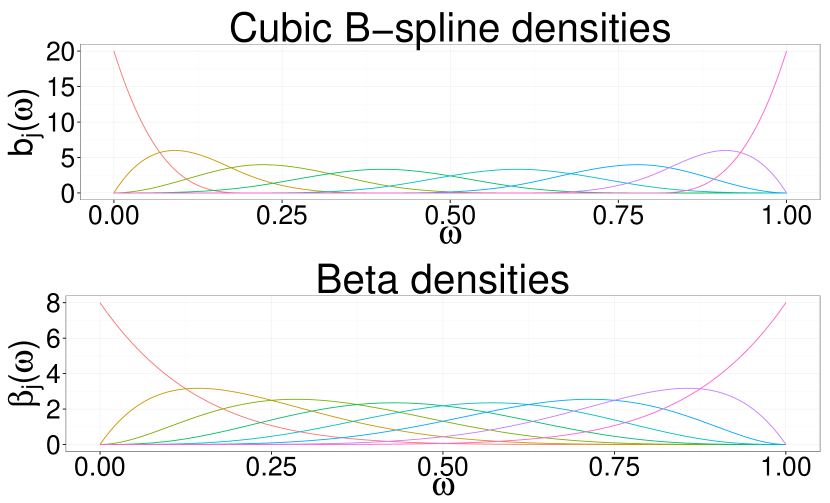
Figure 1: Top panel: Eight cubic B-spline densities with equidistant knots at $\omega=\{0,0.2,0.4,0.6,0.8,1\}$. Notice the local support. Bottom panel: Eight beta densities with full support on the entire unit interval.

When there are no internal knots, the B-spline basis becomes a Bernstein polynomial basis. Bernstein polynomials are thus a special case of B-splines, and the B-spline prior could be regarded as a generalization of the Bernstein polynomial prior.

Figure 2 demonstrates that it is possible to construct curves (B-spline mixtures) with sharp peaks if knots are sufficiently close together. The top panel shows a set of B-spline density functions and the bottom panel displays a mixture of these with random weights. The local support property of B-splines is the reason the B-spline prior will be instrumental in estimating a spectral density with sharp features.

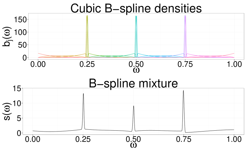
Figure 2: Top panel: Cubic B-spline densities with many knots close to each of the locations $\omega=\{0.25,0.5,0.75\}$. Bottom panel: A random mixture of these B-spline densities. It is possible to construct a B-spline mixture with abrupt, sharp peaks.

2.3 Prior for the spectral density

To place a prior on the spectral density $f(.)$ of a stationary time series defined on the interval $[0,\pi]$, we use the following reparametrization:

$$f(\pi\omega)=\tau\times s_{r}(\omega;k,G,H),\quad\omega\in[0,1],$$ (10)

where $\tau=\int_{0}^{1}f(\pi\omega)\mathrm{d}\omega$ is the normalization constant, and $s_{r}(.)$ is the B-spline prior defined in Equation (9).

The prior for $f(.)$ therefore has the following hierarchical structure:

• $G$ determines the weights (i.e., scale) for each of the $k$ B-spline densities. Let $G\sim\mathrm{DP}(M_{G},G_{0})$, where $M_{G}>0$ is the precision parameter and $G_{0}$ is the base probability distribution function with density $g_{0}$.

• $H$ determines the location of knots and hence the shape and location of the B-spline densities. Let $H\sim\mathrm{DP}(M_{H},H_{0})$, where $M_{H}>0$ is the precision parameter and $H_{0}$ is the base probability distribution function with density $h_{0}$.

• $k$ is the number of B-spline densities in the mixture (i.e., smoothness) and has discrete probability mass function $p(k)\propto\mathrm{exp}(-\theta_{k}k^{2})$ for $k=1,2,\ldots,k_{\mathrm{max}}$. Here $k_{\mathrm{max}}$ is the largest possible value we allow $k$ to take. We limit the maximum value of $k$ for computational reasons and do pilot runs to ensure a larger $k_{\max}$ is not required. A smaller $k$ implies smoother spectral densities.

• $\tau$ is the normalizing constant. Let $\tau\sim\mathrm{IG}(\alpha_{\tau},\beta_{\tau})$.

Assume all of these parameters are a priori independent.

3 Implementation using Markov chain Monte Carlo

As Dirichlet process priors have been placed on $G$ and $H$, we require an algorithm to sample from these distributions. To sample from a Dirichlet process, we use Sethuraman’s stick-breaking construction (Sethuraman, 1994), an infinite-dimensional mixture model. For computational purposes, the number of mixture components for the Dirichlet process representations of $G$ and $H$ is truncated to large but finite positive integers ($L_{G}$ and $L_{H}$ respectively). A larger choice of $L_{G}$ and $L_{H}$ will yield more accurate approximations, but at the expense of increasing the computation time.

To set up the stick-breaking process, reparametrize $G$ to $(Z_{0},Z_{1},\ldots,Z_{L_{G}},V_{1},\ldots,V_{L_{G}})$ such that

$$G = \left(\sum_{l=1}^{L_{G}}p_{l}\delta_{Z_{l}}\right)+\left(1-\sum_{l=1}^{L_{G}}p_{l}\right)\delta_{Z_{0}},$$ (11)

$$p_{1} = V_{1},$$ (12)

$$p_{l} = \left(\prod_{j=1}^{l-1}\left(1-V_{j}\right)\right)V_{l},\quad l\geq 2,$$ (13)

$$p_{0} = 1-\sum_{l=1}^{L_{G}}p_{l},$$ (14)

$$V_{l} \sim \mathrm{Beta}(1,M_{G}),\quad l=1,\ldots,L_{G},$$ (15)

$$Z_{l} \sim G_{0},\quad l=0,1,\ldots,L_{G},$$ (16)

and $H$ to $(X_{0},X_{1},\ldots,X_{L_{H}},U_{1},\ldots,U_{L_{H}})$ such that

$$H = \left(\sum_{l=1}^{L_{H}}q_{l}\delta_{X_{l}}\right)+\left(1-\sum_{l=1}^{L_{H}}q_{l}\right)\delta_{X_{0}},$$ (17)

$$q_{1} = U_{1},$$ (18)

$$q_{l} = \left(\prod_{j=1}^{l-1}\left(1-U_{j}\right)\right)U_{l},\quad l\geq 2,$$ (19)

$$q_{0} = 1-\sum_{l=1}^{L_{H}}q_{l},$$ (20)

$$U_{l} \sim \mathrm{Beta}(1,M_{H}),\quad l=1,\ldots,L_{H},$$ (21)

$$X_{l} \sim H_{0},\quad l=0,1,\ldots,L_{H},$$ (22)

where $\delta_{a}$ is a probability density, degenerate at $a$, i.e., $\delta_{a}=1$ at $a$ and 0 otherwise.

Conditional on $k$, the above hierarchical structure provides a finite mixture prior for the spectral density of a stationary time series

$$f(\pi\omega)=\tau\sum_{j=1}^{k}w_{j,k}b_{j,r}(\omega;\boldsymbol{\xi}),$$ (23)

with weights

$$w_{j,k}=\sum_{l=0}^{L_{G}}p_{l}I\left\{\frac{j-1}{k}<Z_{l}\leq\frac{j}{k}\right\},$$ (24)

and knot differences

$$\Delta_{j} = (\xi_{j+r}-\xi_{j+r-1})$$ (25)

$$= \sum_{l=0}^{L_{H}}q_{l}I\left\{\frac{j-1}{k-r}<X_{l}\leq\frac{j}{k-r}\right\},$$ (26)

for $j=\{1,\ldots,k-r\}$ and $k>r$. The denominator $k-r$ in the latter comes from assuming the exterior knots are the same as the boundary knots. Note also that we assume the lower internal boundary knot $\xi_{r}=0$, meaning the first knot difference is $\Delta_{1}=\xi_{r+1}-\xi_{r}=\xi_{r+1}$. The subsequent knot placements are determined by taking the cumulative sum of the knot differences.

Abbreviating the vector of parameters to $\boldsymbol{\theta}=(\mathbf{v,z,u,x},k,\tau)$, the joint prior is

$$p(\boldsymbol{\theta}) \propto\left(\prod_{l=1}^{L_{G}}M_{G}(1-v_{l})^{M_{G}-1}\right)\left(\prod_{l=0}^{L_{G}}g_{0}(z_{l})\right)$$

$$\quad\times\left(\prod_{l=1}^{L_{H}}M_{H}(1-u_{l})^{M_{H}-1}\right)\left(\prod_{l=0}^{L_{H}}h_{0}(x_{l})\right)$$

$$\quad\times p(k)p(\tau).$$

To produce the unnormalized joint pseudo-posterior, this joint prior is updated using the Whittle likelihood defined in Equation (3).

We implement a Metropolis-within-Gibbs algorithm to sample points from the pseudo-posterior, using the same modular symmetric proposal distributions for B-spline weight parameters $\mathbf{V}$ and $\mathbf{Z}$ as described by Choudhuri et al. (2004). That is, say for $V_{l}$, propose a candidate from a uniform distribution with $[V_{l}-\epsilon_{l},V_{l}+\epsilon_{l}]$, modulo the circular unit interval. If the candidate is greater than 1, take the decimal part only, and if the candidate is less than 0, add 1 to put it back into [0, 1]. This is done for all of the $\mathbf{V}$ and $\mathbf{Z}$ parameters. Choudhuri et al. (2004) found that $\epsilon_{l}=l/(l+2\sqrt{n})$ worked well for most cases, and we also adopt this. The same approach is used analogously for the B-spline knot location parameters $\mathbf{U}$ and $\mathbf{X}$. Parameter $\tau$ has a conjugate inverse-gamma prior and may be sampled directly. Smoothing parameter $k$ could be sampled directly from its discrete full conditional (as done by Choudhuri et al. (2004)), though this can be computationally expensive for large $k_{\max}$, so we use a Metropolis proposal centered on the previous value of $k$, such that there is a 75% chance of jumping according to a discrete uniform on $[-1,1]$, and a 25% chance of boldly jumping according to a discretized Cauchy random variable.

There is a common tendency towards multimodal posteriors in finite/infinite mixture models. If there are many isolated modes separated by low posterior density, it is important to use a sampling technique that mixes Markov chains efficiently, rather than relying on the random walk behaviour of the Metropolis sampler. In order to mitigate poor mixing and to accelerate convergence of Markov chains, we use parallel tempering, or replica exchange (Swendsen and Wang, 1986; Earl and Deem, 2005) for the gravitational wave application in Section 5.2.

The idea of parallel tempering is borrowed from physical chemistry, where a system may be replicated multiple times at a series different temperatures. Higher temperature replicas are able to sample larger volumes of the parameter space, whereas lower temperature replicas may become stuck in local modes. The method works by allowing the exchange of information between neighbouring systems. Information from the high temperature replicas can trickle down to the low temperature systems (including the posterior distribution of interest), providing more representative posterior samples.

In the context of MCMC, parallel tempering involves introducing an auxiliary variable called inverse-temperature, denoted $T_{c}^{-1}$ for chains $c=\{1,2,\ldots,C\}$. This variable becomes an exponent in the target distribution for each parallel chain, $p_{c}(.)$. That is, $p_{c}(\boldsymbol{\theta}|\mathbf{y})^{T_{c}^{-1}}$, where $\boldsymbol{\theta}$ are the model parameters, and $\mathbf{y}$ is the time series data vector. If $T_{c}^{-1}=1$, this is the posterior distribution of interest. All other inverse-temperature values produce tempered target distributions. As $T_{c}\rightarrow\infty$, the target distribution flattens out. Each chain moves on its own in parallel and occasionally swaps states between chains according to the following Metropolis acceptance ratio:

$$\varrho=\left(\frac{p(\boldsymbol{\theta}_{j})p(\mathbf{y}|\boldsymbol{\theta}_{j})}{p(\boldsymbol{\theta}_{i})p(\mathbf{y}|\boldsymbol{\theta}_{i})}\right)^{T_{i}^{-1}-T_{j}^{-1}},$$ (27)

where information is exchanged between chains $i$ and $j$ and $i<j$.

We use cubic B-splines ($r=3$) for all of the examples in the following sections. The serial version of the (cubic) B-spline prior algorithm is available as a function called gibbs_bspline in the R package bsplinePsd (Edwards et al., 2017). This is available on CRAN. The parallel tempered version is implemented in R using the Rmpi library but is not publicly available. Please contact the first author for access to this code.

4 Simulation study

In this section, we run a simulation study on two autoregressive (AR) time series of different order: AR(1) and AR(4). For the first scenario, an AR(1) with first order autocorrelation $\rho_{1}=0.9$ (a relatively simple spectral density) is generated. In the second scenario, an AR(4) with parameters $\rho_{1}~{}=~{}0.9,\rho_{2}~{}=~{}-0.9,\rho_{3}~{}=~{}0.9$, and $\rho_{4}~{}=~{}-0.9$ is generated, such that the spectral density has two large peaks. Let each time series have lengths $n~{}=~{}\{128,~{}256,~{}512\}$ with unit variance Gaussian innovations.

We simulate 1,000 different realizations of AR(1) and AR(4) data and model the spectral densities by running the Bernstein polynomial prior algorithm of Choudhuri et al. (2004) and the B-spline prior algorithm defined in Section 3 on each of these. The MCMC algorithms (without parallel tempering as mixing is satisfactory for these toy examples) run for 400,000 iterations, with a burn-in period of 200,000 and thinning factor of 10, resulting in 20,000 stored samples.

For both spectral density estimation methods, we choose default noninformative priors. That is, for the B-spline prior, let $M_{G}=M_{H}=1,G_{0}\sim\mathrm{Uniform}[0,1],H_{0}\sim\mathrm{Uniform}[0,1],\theta_{k}=0.01,\alpha_{\tau}=\beta_{\tau}=0.001$. For comparability, we let the Bernstein polynomial prior have exactly the same prior set-up as the B-spline prior, but obviously without knot location parameter $M_{H}$ and distribution $H_{0}$.

We set $k_{\mathrm{max}}=500$ for both algorithms. This may seem unnecessarily large for the B-spline prior algorithm as these simple cases converge to a low $k$. However, it is large enough to ensure the Bernstein polynomial algorithm converges to an appropriate $k$, without being truncated at $k_{\max}$.

Based on the suggestions by Choudhuri et al. (2004), we set the stick-breaking truncation parameters to $L_{G}=L_{H}=\max\{20,n^{1/3}\}$. This provides a reasonable balance between accuracy and computational efficiency.

The (cubic) B-spline prior algorithm is run using the gibbs_bspline function in the R package bsplinePsd (Edwards et al., 2017). The Bernstein polynomial prior algorithm is run using the gibbs_NP function in the R package beyondWhittle (Kirch et al., 2017; Meier et al., 2017). Both packages are available on CRAN.

An AR($p$) model has theoretical spectral density,

$$f(\lambda)=\frac{\sigma^{2}}{2\pi}\frac{1}{|1-\sum_{j=1}^{p}\rho_{j}\exp(-\mathrm{i}\lambda)|^{2}},$$ (28)

where $\sigma^{2}$ is the variance of the white noise innovations and $(\rho_{1},\ldots,\rho_{p})$ are the model parameters. We can compare estimates to this true spectral density to measure relative performance of the nonparametric priors. One measure of closeness and accuracy is the integrated absolute error (IAE), also known as the $L_{1}$-error. This is defined as:

$$\mathrm{IAE}=\lVert\hat{f}-f\rVert_{1}=\int_{0}^{\pi}|\hat{f}(\omega)-f(\omega)|d\omega,$$ (29)

where $\hat{f}(.)$ is the Monte Carlo estimate (posterior median) of the spectral density $f(.)$. We calculate the IAE for each replication and then compare the average IAE over all 1,000 replications. The results are presented in Table 1.

Table 1: Median $L_{1}$-error for the estimated spectral densities using B-spline prior and Bernstein polynomial prior on simulated AR(1) and AR(4) data.

AR(1)	$n=128$	$n=256$	$n=512$
B-spline	0.901	0.756	0.592
Bernstein	0.830	0.706	0.518
AR(4)	$n=128$	$n=256$	$n=512$
B-spline	3.242	2.371	1.886
Bernstein	3.427	2.920	2.656

Table 1 compares the median IAE of the estimated spectral densities under the two different nonparametric priors. For the AR(1) cases, the median IAE is only marginally higher for the B-spline prior than the Bernstein polynomial prior. As the AR(1) has a simple spectral structure, this is a case where the global support of the Bernstein polynomials makes sense. However, when estimating the more complicated AR(4) spectral density, we see that the B-spline prior yields more accurate estimates than the Bernstein polynomial prior in terms of IAE. We also see that for both priors, as $n$ increases, median IAE decreases.

For each simulation, we calculate two different credible regions: the usual equal-tailed pointwise credible region, and the uniform (or simultaneous) credible band (Neumann and Polzehl, 1998; Neumann and Kreiss, 1998; Lenhoff et al., 1999; Sun and Loader, 1994). Uniform credible bands are very useful as they allow the calculation of coverage levels for entire curves (spectral densities in this case) rather than pointwise intervals. To compute a $100(1-\alpha)$% uniform credible band, we use the following form:

$$\hat{f}(\lambda)\pm\zeta_{\alpha}\times\mathrm{mad}(\hat{f_{i}}(\lambda)),\quad\lambda\in[0,\pi],$$ (30)

where $\hat{f}(\lambda)$ is the pointwise posterior median spectral density, $\mathrm{mad}(\hat{f_{i}}(\lambda))$ is the median absolute deviation of the posterior samples $\hat{f_{i}}(\lambda)$ kept after burn-in and thinning (which are used as the estimate of dispersion of the sampling distribution of $\hat{f}(\lambda)$), and we choose the $\zeta_{\alpha}$ such that

$$\mathbb{P}\left\{\max\left\{\frac{|\hat{f_{i}}(\lambda)-\hat{f}(\lambda)|}{\mathrm{mad}(\hat{f_{i}}(\lambda))}\right\}\leq\zeta_{\alpha}\right\}=1-\alpha.$$ (31)

Based on these uniform credible bands, uniform coverage probabilities over all 1,000 replications of the simulation can be computed. That is, calculate the proportion of times that the true spectral density is entirely encapsulated within the uniform credible band. Computed coverage probabilities are shown in Table 2.

Table 2: Coverage probabilities based on 90% uniform credible bands.

AR(1)	$n=128$	$n=256$	$n=512$
B-spline	1.000	1.000	0.998
Bernstein	1.000	0.987	0.499
AR(4)	$n=128$	$n=256$	$n=512$
B-spline	0.936	0.979	0.907
Bernstein	0.000	0.000	0.000

It can be seen in Table 2 that the B-spline prior has higher coverage than the Bernstein polynomial prior in all examples (apart from the AR(1) with $n=128$, where it is the same). The B-spline prior produces excellent coverage probabilities for the AR(1) cases. The Bernstein polynomial prior also performs well in this regard, apart from the $n=512$ case, where half are not fully covered. An example from one of the 1,000 replications of the AR(1) with $n=512$ is given in Figure 3. Here, the uniform credible band fully contains the true PSD for the B-spline prior but not for the Bernstein polynomial prior (the true PSD falls outside the uniform credible band at the highest frequencies). The pointwise credible region and posterior median log-PSD for both priors are also very accurate. This is not surprising as the AR(1) has a relatively simple spectral structure.

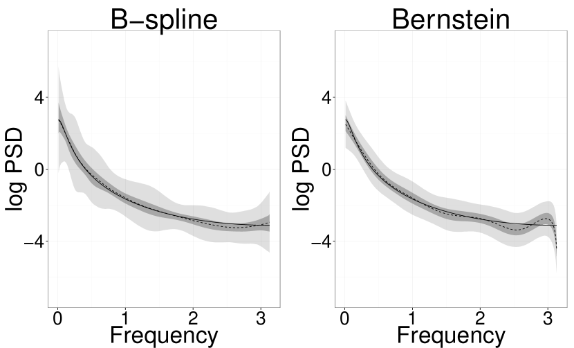
Figure 3: Estimated log-spectral densities for an AR(1) time series using the B-spline prior (left) and Bernstein polynomial prior (right). The solid line is the true log-PSD; the dashed line is the posterior median log-PSD; the dark shaded region is the pointwise 90% credible region; and the light shaded region is the uniform 90% credible band.

Coverage of the AR(4) spectral density under the B-spline prior is above 90% for each sample size. However, the Bernstein polynomial prior has extremely poor coverage in the AR(4) case, where none of the 1,000 replications are fully covered by the uniform credible band for each sample size. An example of this performance (for $n=512$) can be seen in Figure 4. The Bernstein polynomial prior (under the noninformative prior set-up) tends to poorly estimate the second large peak of the PSD, and introduces additional incorrect peaks and troughs throughout the rest of estimate. These false peaks and troughs are present due to the Bernstein polynomial prior algorithm converging to large $k$ in an attempt to approximate the two large peaks of the AR(4) PSD. The B-spline prior gives a much more accurate Monte Carlo estimate. The posterior median log-PSD is close to the true AR(4) PSD, the 90% pointwise credible region mostly contains the true PSD, and the 90% uniform credible band fully contains it.

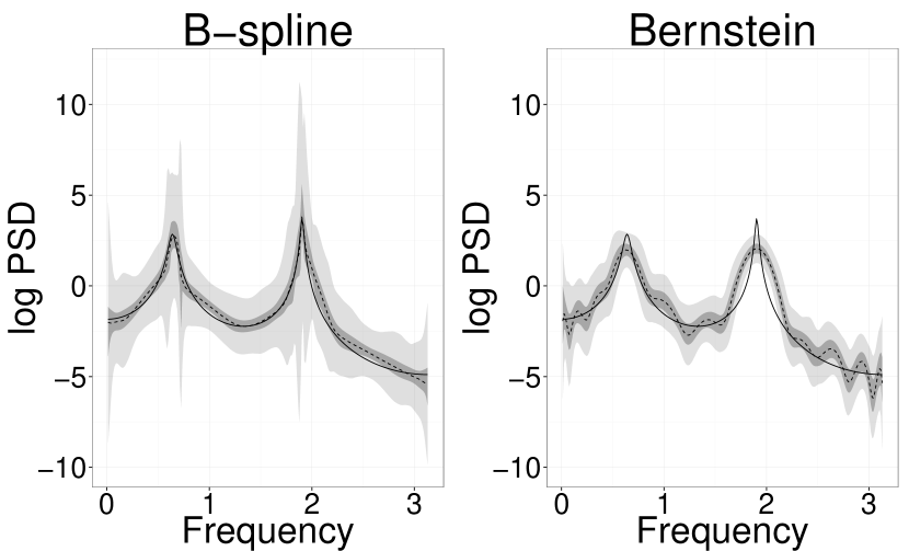
Figure 4: Estimated log-spectral densities for an AR(4) time series using the B-spline prior (left) and Bernstein polynomial prior (right). The solid line is the true log-PSD; the dashed line is the posterior median log-PSD; the dark shaded region is the pointwise 90% credible region; and the light shaded region is the uniform 90% credible band.

Of course, the Bernstein polynomial prior could perform better on spectral densities with sharp features if significant prior knowledge was known in advance. This can however be a formidable task, and is not very generalizable to other time series. A benefit of using the B-spline prior is its ability to estimate a variety of different spectral densities using the default noninformative priors used in this paper. We will see more examples of this in Section 5.

One slight drawback of the B-spline prior algorithm is its computational complexity relative to the Bernstein polynomial prior. B-spline densities must be evaluated many times per MCMC iteration (when sampling $k,\mathbf{U}$, and $\mathbf{X}$) due to the variable knot placements, whereas beta densities can be pre-computed and stored in memory, saving much computation time.

Table 3 displays the median run-time (over each 1,000 replication) for each of the six AR simulations.

Table 3: Median absolute run-times (hours) and their associated relative run-times.

AR(1)	$n=128$	$n=256$	$n=512$
B-spline	2.967	3.186	3.659
Bernstein	1.423	1.572	1.844
B-spline/Bernstein	2.086	2.026	1.985
AR(4)	$n=128$	$n=256$	$n=512$
B-spline	4.044	4.422	5.174
Bernstein	1.443	1.694	2.281
B-spline/Bernstein	2.802	2.610	2.268

It can be seen in Table 3 that the B-spline prior algorithm is approximately 2–3 times slower than the Bernstein polynomial prior algorithm for these examples. Due to the noted advantages that the B-spline prior has over the Bernstein polynomial prior (such as accuracy and coverage), particularly for PSDs with complicated structures, the increased computation time is an acceptable trade-off, though for simple spectral densities, the Bernstein polynomial prior should suffice.

5 Applications in astronomy

5.1 Annual sunspot numbers

In this section, we analyze the annual mean sunspot numbers from 1700 to 1987. Sunspots are darker and cooler regions of the Sun’s surface caused by magnetic fields penetrating the surface from below. Sunspots are linked to various solar phenomena such as solar flares and the auroras.

Previous analyses have shown that the sunspot (or solar) cycle reaches a solar maximum approximately every 11 years (see e.g., Schwabe (1843) for the original reference and Choudhuri et al. (2004) for analysis using the Bernstein polynomial prior). The analysis in this section is consistent with this claim.

As done by Choudhuri et al. (2004), we first transform the data by taking the square root of the original 288 observations to make the data stationary. We then mean-center the resulting data.

The serial version of the B-spline prior MCMC algorithm is run for 100,000 iterations, with a burn-in period of 50,000 and thinning factor of 10, resulting in 5,000 stored samples. This takes approximately 40 minutes to run. All other specifications are the same as in Section 4. An estimate of the PSD is displayed in Figure 5.

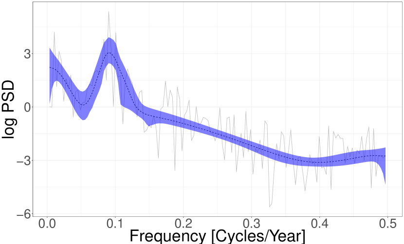
Figure 5: Estimated log-PSD for the annual mean sunspot numbers from 1700 to 1987. The posterior median log-PSD (dashed black) along with the 90% pointwise credible region (shaded blue) are overlaid with the log-periodogram (grey).

It can be seen in Figure 5 that a spectral peak occurs at the frequency of 0.0903 cycles per year. This is equivalent to a solar cycle every 11.07 years, consistent with existing knowledge.

5.2 Recoloured LIGO gravitational wave data

Gravitational waves (GWs) are ripples in the fabric of spacetime, caused by the most exotic and cataclysmic astrophysical events in the cosmos, such as binary black hole or neutron star mergers, core collapse supernovae, pulsars, and even the Big Bang. They are a consequence of Einstein’s general theory of relativity (Einstein, 1916).

On September 14, 2015, the breakthrough first direct detection of GWs was made using the Advanced LIGO detectors (Abbott et al., 2016a). The signal, GW150914, came from a pair of stellar mass black holes that coalesced approximately 1.3 billion light-years away. This was also the first direct observation of black hole mergers. Four subsequent detections of pairs of stellar mass black holes have been made (Abbott et al., 2016b, 2017b, 2017c, 2017d), as well as the first binary neutron star detection with an electromagnetic counterpart (Abbott et al., 2017a), signalling a new era of astronomy is now upon us.

Advanced LIGO is a set of two GW interferometers in the United States (one in Hanford, Washington, and the other in Livingston, Louisiana) (Aasi et al., 2015). Data collected by these observatories are dominated by instrument and background noise — primarily seismic, thermal, and photon shot noise. There are also high power, narrow band, spectral noise lines caused by the AC electrical supplies and mirror suspensions, among other phenomena. Though GW150914 had a large signal-to-noise ratio, signals detected by these observatories will generally be relatively weak. Improving the characterization of detector/background noise could therefore positively impact signal characterization and detection confidence.

The default noise model in the gravitational wave literature assumes instrument noise is Gaussian, stationary, and has a known PSD. Real data often depart from these assumptions, motivating the development of alternative statistical models for detector noise. In the literature, this includes Student-t likelihood generalizations by Röver et al. (2011) and Röver (2011), introducing additional scale parameters and marginalization by Littenberg et al. (2013) and Vitale et al. (2014), modelling the broadband PSD with a cubic spline and spectral lines with Cauchy random variables by Littenberg and Cornish (2015), and the use of a Bernstein polynomial prior by Edwards et al. (2015).

We found that due to the undesirable properties of the Bernstein polynomial prior, it was not flexible enough to estimate sharp peaks in the spectral density of real LIGO noise. This, coupled with the fact that B-splines have local support, provided the rationale for implementing the B-spline prior instead.

In the following example, using the parallel tempered B-spline prior algorithm, we estimate the PSD of a 1 s stretch of real LIGO data collected during the sixth science run (S6), recoloured to match the target noise sensitivity of Advanced LIGO (Christensen, 2010). LIGO has a sampling rate of 16384 Hz. To reduce the volume of data processed, a low-pass Butterworth filter (of order 10 and attenuation 0.25) is applied, then the data are downsampled to 4096 Hz (resulting in a sample size of $n=4096$). Prior to downsampling, the data are differenced once to become stationary, mean-centered, and then Hann windowed to mitigate spectral leakage. Though a 1 s stretch may seem small in the context of GW data analysis, this time scale is important for on-source characterization of noise during short-duration transient events, called bursts (Abadie et al., 2012). This is particularly true since LIGO noise has a time-varying spectrum, and systematic biases could occur if off-source noise was used to estimate the power spectrum of on-source noise.

We run 16 parallel chains (each at different temperatures) of the MCMC algorithm for $400,000$ iterations, with a burn-in of $200,000$ and thinning factor of 5, yielding $40,000$ stored samples. We propose swaps (of all parameters blocked together) between adjacent chains on every tenth iteration. For each chain $c$, we found the following inverse-temperature scheme gave reasonable results:

$$T_{c}^{-1}=T_{\mathrm{min}}^{-\Delta_{c}},$$ (32)

where $T_{\mathrm{min}}=0.005$ is the minimum inverse-temperature allowed, $\Delta_{c}=\frac{c-1}{C-1}$, and $C=16$ is the number of chains. The stick-breaking truncation parameters are set to $L_{G}=L_{H}=20$ and all of the other prior specifications are exactly the same as used in the AR simulation study of Section 4. Note that as the sample size for this example is very large ($n=4096$), the algorithm took several hours to run.

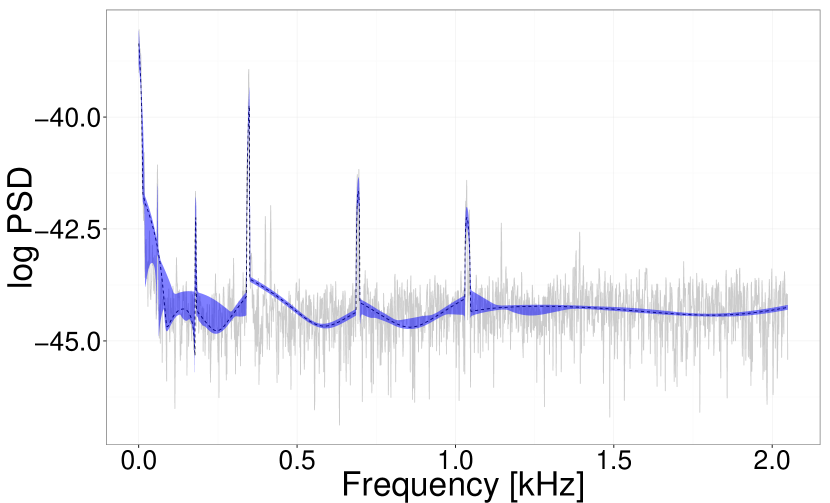
Figure 6: Estimated $\mathrm{log}_{10}$-PSD for a 1 s segment of recoloured LIGO S6 data. The posterior median log-PSD (dashed black) along with the 90% pointwise credible region (shaded blue) are overlaid with the log-periodogram (grey). The log transform is base 10 here.

As demonstrated in Section 4 (e.g., Figure 4), the Bernstein polynomial approach would have struggled to estimate the abrupt changes of power present in real detector data. It can be seen in Figure 6 though, that the B-spline approach estimates the log-spectral density very well. The estimated log-PSD follows the general broad-band shape of the log-periodogram well, and the primary sharp changes in power are also accurately estimated. The method, however, seems to be less sensitive to some of the smaller spikes.

6 Conclusions and outlook

In this paper, we have presented a novel approach to spectral density estimation, using a nonparametric B-spline prior with a variable number and location of knots. We have demonstrated that for complicated PSDs, this method outperforms the Bernstein polynomial prior in terms of IAE and uniform coverage probabilities.

The B-spline prior provides superior Monte Carlo estimates, particularly for spectral densities with sharp and abrupt changes in power. This is not surprising as B-splines have local support and better approximation properties than Bernstein polynomials. However, the favourable estimation qualities of the B-spline prior come at the expense of increased computation time.

The posterior distribution of the B-spline mixture parameters with variable number and location of knots could be sampled using the RJMCMC algorithm of Green (1995), however RJMCMC methods are often fraught with implementation difficulties, such as finding efficient jump proposals when there are no natural choices for trans-dimensional jumps (Brooks et al., 2003). We avoid this altogether by allowing for a data-driven choice of the smoothing parameter and knot locations using the nonparametric Dirichlet process prior. This yields a much more straightforward sampling mechanism.

The B-spline prior was applied to the annual mean sunspot data set. We got a reasonable estimate of the log-PSD, and estimated that the solar cycle occurs every 11.07 years. This is consistent with existing knowledge and previous analyses.

We have demonstrated that the B-spline prior provides a reasonable estimate of the spectral density of real instrument noise from the LIGO gravitational wave detectors. In a future paper, we will focus on characterizing this noise while simultaneously extracting a GW signal, similar to Edwards et al. (2015). As the algorithm is computationally expensive, it will be well-suited towards the shorter burst-type signals (of order 1 s or less) like rotating core collapse supernovae. Using a large enough catalogue of waveforms, estimation of astrophysically meaningful parameters could be done by sampling from the posterior predictive distribution, similar to Edwards et al. (2014). Another future initiative is to analyze the impact of informative priors on the LIGO PSD estimates.

Though we have only presented the B-spline prior in terms of spectral density estimation, it could be used in a much broader context, such as in density estimation. A paper using this approach for density estimation is in preparation and could yield a more flexible, alternative approach to the Triangular-Dirichlet prior function TDPdensity in the R package DPpackage (Jara et al., 2011).

References

- Aasi et al. [2015] J. Aasi et al. Advanced LIGO. Classical and Quantum Gravity, 32:074001, 2015.
- Abadie et al. [2012] J. Abadie et al. All-sky search for gravitational-wave bursts in the second joint LIGO-Virgo run. Physical Review D, 85:122007, 2012.
- Abbott et al. [2016a] B. P. Abbott et al. Observation of gravitational waves from a binary black hole merger. Physical Review Letters, 116:061102, 2016a.
- Abbott et al. [2016b] B. P. Abbott et al. GW151226: Observation of gravitational waves from a 22-solar-mass binary black hole coalescence. Physical Review Letters, 116:241103, 2016b.
- Abbott et al. [2017a] B. P. Abbott et al. GW170817: Observation of gravitational waves from a binary neutron star inspiral. Physical Review Letters, 119:161101, 2017a.
- Abbott et al. [2017b] B. P. Abbott et al. GW170104: Observation of a 50-solar-mass binary black hole coalescence at redshift 0.2. Physical Review Letters, 118:221101, 2017b.
- Abbott et al. [2017c] B. P. Abbott et al. GW170814: A three-detector observation of gravitational waves from a binary black hole coalescence. Physical Review Letters, 119:141101, 2017c.
- Abbott et al. [2017d] B. P. Abbott et al. GW170608: Observation of a 19-solar-mass binary black hole coalescence. Pre-print, arXiv:1711.05578 [astro-ph.HE], 2017d.
- Acernese et al. [2015] F. Acernese et al. Advanced Virgo: A second-generation interferometric gravitational wave detector. Classical and Quantum Gravity, 32(2):024001, 2015.
- Barnett et al. [1996] G. Barnett, R. Kohn, and S. Sheather. Bayesian estimation of an autoregressive model using Markov chain Monte Carlo. Journal of Econometrics, 74:237–254, 1996.
- Bartlett [1950] M. S. Bartlett. Periodogram analysis and continuous spectra. Biometrika, 37:1–16, 1950.
- Brockwell and Davis [1991] P. J. Brockwell and R. A Davis. Time Series: Theory and Methods. Springer, New York, 2nd edition, 1991.
- Brooks et al. [2003] S. P. Brooks, P. Giudici, and G. O. Roberts. Efficient construction of reversible jump Markov chain Monte Carlo proposal distributions. Journal of the Royal Statistical Society: Series B (Methodological), 65:3–55, 2003.
- Cai and Meyer [2011] B. Cai and R. Meyer. Bayesian semiparametric modeling of survival data based on mixtures of B-spline distributions. Computational Statistics and Data Analysis, 55:1260–1272, 2011.
- Carter and Kohn [1997] C. K. Carter and R. Kohn. Semiparametric Bayesian inference for time series with mixed spectra. Journal of the Royal Society, Series B, 59:255–268, 1997.
- Chopin et al. [2013] N. Chopin, J. Rousseau, and B. Liseo. Computational aspects of Bayesian spectral density estimation. Journal of Computational and Graphical Statistics, 22:533–557, 2013.
- Choudhuri et al. [2004] N. Choudhuri, S. Ghosal, and A. Roy. Bayesian estimation of the spectral density of a time series. Journal of the American Statistical Association, 99(468):1050–1059, 2004.
- Christensen [2010] N. Christensen. LIGO S6 detector characterization studies. Classical and Quantum Gravity, 27:194010, 2010.
- Cogburn and Davis [1974] R. Cogburn and H. R. Davis. Periodic splines and spectral estimation. The Annals of Statistics, 2:1108–1126, 1974.
- Crandell and Dunson [2011] J. L. Crandell and D. B. Dunson. Posterior simulation across nonparametric models for functional clustering. Sankhya B, 73:42–61, 2011.
- de Boor [1993] C. de Boor. B(asic)-spline basics, in: L. Piegl (Ed.), Fundamental developments of computer-aided geometric modeling. Academic Press, Washington, DC, 1993.
- Earl and Deem [2005] D. J. Earl and M. W. Deem. Parallel tempering: Theory, applications, and new perspectives. Physical Chemistry Chemical Physics, 7:3910–3916, 2005.
- Edwards et al. [2014] M. C. Edwards, R. Meyer, and N. Christensen. Bayesian parameter estimation of core collapse supernovae using gravitational wave signals. Inverse Problems, 30:114008, 2014.
- Edwards et al. [2015] M. C. Edwards, R. Meyer, and N. Christensen. Bayesian semiparametric power spectral density estimation with applications in gravitational wave data analysis. Physical Review D, 92:064011, 2015.
- Edwards et al. [2017] M. C. Edwards, R. Meyer, and N. Christensen. bsplinePsd: Bayesian power spectral density estimation using B-spline priors. R package, 2017.
- Einstein [1916] A. Einstein. Approximative integration of the field equations of gravitation. Sitzungsberichte Preußischen Akademie der Wissenschaften, 1916 (Part 1):688–696, 1916.
- Gangopadhyay et al. [1999] A. K. Gangopadhyay, B. K. Mallick, and D. G. T. Denison. Estimation of the spectral density of a stationary time series via an asymptotic representation of the periodogram. Jounal of Statistical Planning and Inference, 75:281–290, 1999.
- Gelman et al. [2013] A. Gelman, J. B. Carlin, H. S. Stern, D. B. Dunson, A. Vehtari, and D. B. Rubin. Bayesian Data Analysis. Chapman & Hall / CRC, Boca Raton, FL, 3rd edition, 2013.
- Geman and Geman [1984] S. Geman and D. Geman. Stochastic relaxation, Gibbs distributions, and the Bayesian restoration of images. IEEE Trans. Patt. Anal. Mach. Intell., 6:721–741, 1984.
- Green [1995] P. J. Green. Reversible jump Markov chain Monte Carlo computation and Bayesian model determination. Biometrika, 82:711–732, 1995.
- Hastings [1970] W. K. Hastings. Monte Carlo sampling methods using Markov chains and their applications. Biometrika, 57:97–109, 1970.
- Jara et al. [2011] A. Jara, T. E. Hanson, F. A. Quintana, P. Müller, and G. L Rosner. DPpackage: Bayesian semi- and nonparametric modeling in R. Journal of Statistical Software, 40:1–30, 2011.
- Kirch et al. [2017] C. Kirch, M. C. Edwards, A. Meier, and R. Meyer. Beyond Whittle: Nonparametric correction of a parametric likelihood with a focus on Bayesian time series analysis. Pre-print, arXiv:1701.04846v1 [stat.ME], 2017.
- Kooperberg et al. [1995] C. Kooperberg, C. J. Stone, and Y. K. Truong. Rate of convergence for logspline spectral density estimation. Journal of Time Series Analysis, 16:389–401, 1995.
- Lenhoff et al. [1999] M. W. Lenhoff, T. J. Santner, J. C. Otis, M. G. Peterson, B. J. Williams, and S. I. Backus. Bootstrap prediction and confidence bands: A superior statistical method for the analysis of gait data. Gait and Posture, 9:10–17, 1999.
- Liseo et al. [2001] B. Liseo, D. Marinucci, and L. Petrella. Bayesian semiparametric inference on long-range dependence. Biometrika, 88:1089–1104, 2001.
- Littenberg and Cornish [2015] T. B. Littenberg and N. J. Cornish. Bayesian inference for spectral estimation of gravitational wave detector noise. Physical Review D, 91:084034, 2015.
- Littenberg et al. [2013] T. B. Littenberg, M. Coughlin, B. Farr, and Farr W. M. Fortifying the characterization of binary mergers in LIGO data. Physical Review D, 88:084044, 2013.
- Macaro [2010] C. Macaro. Bayesian non-parametric signal extraction for Gaussian time series. Journal of Econometrics, 157:381–395, 2010.
- Macaro and Prado [2014] C. Macaro and R. Prado. Spectral decompositions of multiple time series: A Bayesian non-parametric approach. Psychometrika, 79:105–129, 2014.
- Meier et al. [2017] A. Meier, C. Kirch, M. C. Edwards, and R. Meyer. beyondWhittle: Bayesian spectral inference for stationary time series. R package, 2017.
- Metropolis et al. [1953] N. Metropolis, A. W. Rosenbluth, MN Rosenbluth, A. H. Teller, and Teller E. Equation of state calculations by fast computing machines. J. Chem. Phys., 21:1087–1092, 1953.
- Neumann and Kreiss [1998] M. H. Neumann and J-P Kreiss. Regression-type inference in nonparametric regression. The Annals of Statistics, 26:1570–1613, 1998.
- Neumann and Polzehl [1998] M. H. Neumann and J. Polzehl. Simultaneous bootstrap confidence bands in nonparametric regression. Journal of Nonparametric Statistics, 9:307–333, 1998.
- Perron and Mengersen [2001] F. Perron and K. Mengersen. Bayesian nonparametric modeling using mixtures of triangular distributions. Biometrics, 57:518–528, 2001.
- Petrone [1999a] S. Petrone. Random Bernstein polynomials. Scandanavian Journal of Statistics, 26:373–393, 1999a.
- Petrone [1999b] S. Petrone. Bayesian density estimation using Bernstein polynomials. Canadian Journal of Statistics, 27:105–126, 1999b.
- Powell [1981] M. J. D. Powell. Approximation theory and methods. Cambridge University Press, Cambridge, 1981.
- Rosen et al. [2012] O. Rosen, S. Wood, and A. Roy. AdaptSpec: Adaptive spectral density estimation for nonstationary time series. Journal of the American Statistical Association, 107:1575–1589, 2012.
- Rousseau et al. [2012] J. Rousseau, N. Chopin, and B. Liseo. Bayesian nonparametric estimation of the spectral density of a long or intermediate memory Gaussian time series. The Annals of Statistics, 40:964–995, 2012.
- Röver [2011] C. Röver. Student-t based filter for robust signal detection. Physical Review D, 84:122004, 2011.
- Röver et al. [2011] C. Röver, R. Meyer, and N. Christensen. Modelling coloured residual noise in gravitational-wave signal processing. Classical and Quantum Gravity, 28:015010, 2011.
- Schwabe [1843] S. H. Schwabe. Sonnenbeobachtungen im jahre 1843. Astronomische Nachrichten, 21:233–236, 1843.
- Sethuraman [1994] J. Sethuraman. A constructive definition of Dirichlet priors. Statistica Sinica, 4:639–650, 1994.
- Sun and Loader [1994] J. Sun and C. R. Loader. Confidence bands for linear regression and smoothing. The Annals of Statistics, 22:1328–1345, 1994.
- Swendsen and Wang [1986] R. H. Swendsen and J. S. Wang. Replica Monte Carlo simulation of spin glasses. Physical Review Letters, 57:2607–2609, 1986.
- Thomson [1982] D. J. Thomson. Spectrum estimation and harmonic analysis. Proceedings of the IEEE, 70:1055–1096, 1982.
- Tonellato [2007] S. F. Tonellato. Random field priors for spectral density functions. Journal of Statistical Planning and Inference, 137:3164–3176, 2007.
- Vitale et al. [2014] S. Vitale, G. Congedo, R. Dolesi, V. Ferroni, M. Hueller, D. Vetrugno, W. J. Weber, H. Audley, K. Danzmann, I. Diepholz, M. Hewitson, N. Korsakova, L. Ferraioli, F. Gibert, N. Karnesis, M. Nofrarias, H. Inchauspe, E. Plagnol, O. Jennrich, P. W. McNamara, M. Armano, J. I. Thorpe, and P. Wass. Data series subtraction with unknown and unmodeled background noise. Physical Review D, 90:042003, 2014.
- Wahba [1980] G. Wahba. Automatic smoothing of the log periodogram. Journal of the American Statistical Association, 75:122–132, 1980.
- Welch [1967] P. D. Welch. The use of fast Fourier transform for the estimation of power spectra: A method based on time averaging over short, modified periodograms. IEEE Transactions on Audio and Electroacoustics, 15:70–73, 1967.
- Whittle [1957] P. Whittle. Curve and periodogram smoothing. Journal of the Royal Statistical Society: Series B (Methodological), 19:38–63, 1957.
- Zheng et al. [2010] Y. Zheng, J. Zhu, and A. Roy. Nonparametric Bayesian inference for the spectral density function of a random field. Biometrika, 97:238–245, 2010.