First Principles Study of the Giant Magnetic Anisotropy Energy in Bulk Na₄IrO₄

Abstract

In $5d$ transition metal oxides, novel properties arise from the interplay of electron correlations and spin–orbit interactions. Na₄IrO₄, where $5d$ transition-metal Ir atom occupies the center of the square-planar coordination environment, is synthesized. Based on density functional theory, we calculate its electronic and magnetic properties. Our numerical results show that the Ir-$5d$ bands are quite narrow, and the bands around the Fermi level are mainly contributed by $d_{xy},d_{yz}$ and $d_{zx}$ orbitals. The magnetic easy-axis is perpendicular to the IrO₄ plane, and the magnetic anisotropy energy (MAE) of Na₄IrO₄ is found to be very giant. We estimate the magnetic parameters by mapping the calculated total energy for different spin configurations onto a spin model. The next nearest neighbor exchange interaction $J_{2}$ is much larger than other intersite exchange interactions and results in the magnetic ground state configuration. Our study clearly demonstrates that the huge MAE comes from the single-ion anisotropy rather than the anisotropic interatomic spin exchange. This compound has a large spin gap but very narrow spin-wave dispersion, due to the large single-ion anisotropy and relatively small exchange couplings. Noticing this remarkable magnetic feature originated from its highly isolated IrO₄ moiety, we also explore the possiblity to further enhance the MAE.

I Introduction

It is well known that the Coulomb interaction is of substantial importance in $3d$ electron systems, while the spin-orbit coupling (SOC) in these compounds is quite small 3d-1 ; 3d-2 . However, the SOC and electronic correlation in $5d$ electrons have comparable magnitudes. The delicate interplay between electronic interactions, strong SOC, and crystal field splitting can result in strongly competing ground states in these materials Rev-5d-1 ; Rev-5d-2 ; Rev-5d-3 . Thus recently, $5d$ transition metal (especially Ir or Os) oxides have attracted intensive interest and a great number of exotic phenomena have been observed experimentally or proposed theoretically, e.g. $J_{eff}$=1/2 Mott state J-1/2 1 ; J-1/2 2 ; J-1/2 3 , topological insulator TI-5d-1 ; TI-5d-2 ; TI-5d-3 , Kitaev model Kitav , Weyl Semimetal WSM , high $T_{c}$ superconductivity HTC-214 , Axion insulator Axion-Insulator , quantum spin liquid QSL-1 ; QSL-2 , Slater insulator Slater-1 ; Slater-2 ; Slater-3 , ferroelectric metal FE-Metal-1 ; FE-Metal-2 , etc.

In all the aforementioned systems, the $5d$ ions lie in the octahedral environment of the O ions. In addition to this common coordination geometry, Na₄IrO₄, where Ir atom occupies the center of the square-planar coordination environment, has also been synthesized str . By using density function theory (DFT) calculations, Kanungo 414 et al. reveal that the relative weak Coulomb repulsion of Ir ions plays a key role in the stabilization of the ideal square-planar geometry of the IrO₄ moiety in Na₄IrO₄. Located at the center of an ideally square-planar IrO₄ oxoanion, the $5d$ electrons of Ir ions in Na₄IrO₄ do not display the $J_{eff}$=1/2 configuration 414 . Moreover, the common $5d$ transition metal oxides own face (or edge, corner)-sharing structure of oxygen octahedrons, while the square-planar IrO₄ oxoanion in Na₄IrO₄ is quite isolated. Therefore, exploring the possible exotic properties of Na₄IrO₄ is an interesting study.

In this work, based on first principle calculations, we systematically study the electronic and magnetic properties of Na₄IrO₄. Our numerical results show that the Ir-$5d$ bands are quite narrow, and the bands around the Fermi level are mainly contributed by $d_{xy}$, $d_{yz}$ and $d_{zx}$ orbitals. Due to the isolated IrO₄ moiety, the magnetic moments are quite localized. We calculate several magnetic structures and find that the antiferromagnetic-1 (AFM-1) state as shown in Fig. 4 is the ground state configuration. The interatomic exchange interactions are estimated and the nearest-neighbor $J_{2}$ (shown in Fig. 1) dominates over the others. We find that there is a huge magnetic anisotropy energy (MAE) due to the special square-planar coordination environment and the long distance between IrO₄ moieties. We find the anisotropy of interatomic spin exchange couplings is relatively small, and the huge MAE comes from the single-ion anisotropy. We suggest that substituting Ir by Re atom can further enhance the MAE significantly.

II Method and Crystal structure

The electronic band structure and density of states calculations have been carried out by using the full potential linearized augmented plane wave method as implemented in Wien2k package wien2k . Local spin density approximation (LSDA) is widely used for various $4d$ and $5d$ TMOs J-1/2 1 ; J-1/2 2 ; WSM ; Axion-Insulator ; LSDA-4d , and we therefore adopt it as the exchange-correlation potential. A 9$\times$9$\times$15 k-point mesh is used for the Brillouin zone integral. Using the second-order variational procedure, we include the SOC socref , which has been found to play an important role in the $5d$ system. The self-consistent calculations are considered to be converged when the difference in the total energy of the crystal does not exceed 0.01 mRy. Despite the fact that the $5d$ orbitals are spatially extended, recent theoretical and experimental work has given evidence on the importance of Coulomb interactions in $5d$ compounds Rev-5d-1 ; Rev-5d-2 ; Rev-5d-3 . We utilize the LSDA + $U$ scheme LDA+U to take into account the effect of Coulomb repulsion in $5d$ orbital. We vary the parameter $U$ between 2.0 and 3.0 eV and find that the essential properties are independent on the value of $U$.

As shown in Fig. 1, Na₄IrO₄ crystallizes in the tetragonal structure (space group I4/m) str . The lattice constants of Na₄IrO₄ are $a$ = 7.17 Å and $c$ = 4.71 Åstr . There is only one formula unit in the primitive unit cell, and the nine atoms in the unit cell are located at three nonequivalent crystallographic sites: Ir atoms occupy the $2a$ position: (0,0,0), while both Na and O reside at the $8h$ sites: $(x,y,z)$str . The square-planar IrO₄ oxoanion occurs in the $ab$-plane, and is slightly rotated about the $c$ axis str . The Ir ions occupy the center of the square-planar coordination environment. The average distance of four Ir-O bonds in the square-planar IrO₄ is 1.91 Å, which is similar to the Ir-O bond length in IrO₆ octahedron. Instead of the face (or edge, corner)-sharing structure of octahedrons, the IrO₄ moiety is quite isolated as shown in Fig. 1, thus the Ir-Ir distance is quite large. These remarkable structural features significantly affect the electronic structure and magnetic properties of Na₄IrO₄ as shown in the following sections.

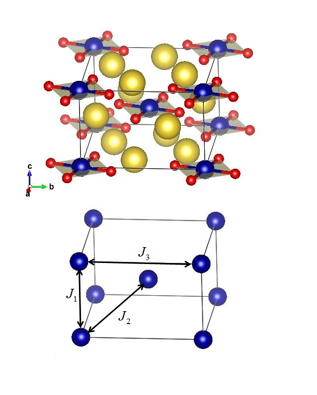
Figure 1: Crystal structure of Na₄IrO₄. The yellow, blue, and red balls represent the Na, Ir, and O ions, respectively. The nearest-neighbor, next-nearest-neighbor and third-nearest-neighbor exchange interactions for Ir magnetic moments are shown by $J_{1}$, $J_{2}$, $J_{3}$ respectively, which are the parameters in the Heisenberg model $H=\sum_{i<j}J_{ij}S_{i}\cdot S_{j}.$

III Band structures

To clarify the basic electronic features, we perform nonmagnetic LDA calculation, and show the band structures and the density of states (DOS) in Fig. 2(a) and Fig. 3, respectively. As shown in Fig. 3, that O-$2p$ states are mainly located between -7.0 and -1.0 eV while the Na $3s$ and $3p$ bands appear mainly above 3.0 eV which is much higher than the Fermi level and also appear between -7.0 and -1.0 eV contributed mainly by the O-$2p$ states, indicating the non-negligible hybridization between Na and O states despite that Na is highly ionic. Hence the chemical valence for Na is $+1$ while that for O is $-2$. As a result, the nominal valence of Ir in Na₄IrO₄ is +4, and the electronic configuration of Ir ion is $5d^{5}$. It is well known that in the octahedral environment the $5d$ orbitals will split into the $t_{2g}$ and $e_{g}$ states, and the strong SOC in $5d$ electrons splits the $t_{2g}$ states into $J_{eff}$ = 1/2 and $J_{eff}$ = 3/2 bands J-1/2 1 ; J-1/2 2 . Compared with the IrO₆ octahedra, the upper and lower O^2- ions are absent in the square-planar IrO₄ oxoanion. Consequently the Ir-5$d$ orbitals split into three non-degenerate orbitals: $d_{3z^{2}-r^{2}},\ d_{xy},\ d_{x^{2}-y^{2}}$, and doubly degenerate $d_{xz}/d_{yz}$ ones. There are in total 13 bands in the energy range from -7.0 eV to -1.0 eV, as shown in Fig. 2(a). The $d_{3z^{2}-r^{2}}$ states appear mainly between -3.0 eV to -2.0 eV, while the remaining 12 bands are contributed by O-$2p$ states. Mainly located above 4 eV, $d_{x^{2}-y^{2}}$ states have also large distribution around -6.5 eV due to the strong hybridization with O-$2p$ bands. The $d_{xz}/d_{yz}$ and $d_{xy}$ orbitals are mainly located from -1.0 to 1.0 eV, while the $d_{xy}$ state is slightly higher in energy. As shown in Fig. 2(a) and Fig. 3, these bands are separated from other bands, and around the Fermi level the orbital splitting can be displayed by the left panel of Fig. 6. The dispersion of the $5d$ bands around Fermi level is very narrow, due to that the IrO₄ moiety is quite isolated in the crystal structure. As shown in Fig. 3, the DOS at Fermi level is rather high, which indicates the magnetic instability.

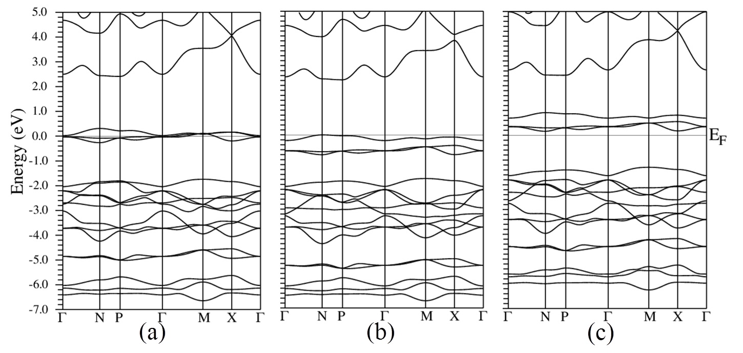
Figure 2: Band structures of Na₄IrO₄. (a) represents the LDA calculation while (b) and (c) represent spin-up and spin-down channel from LSDA calculation with FM configuration. The Fermi energy is set to zero.

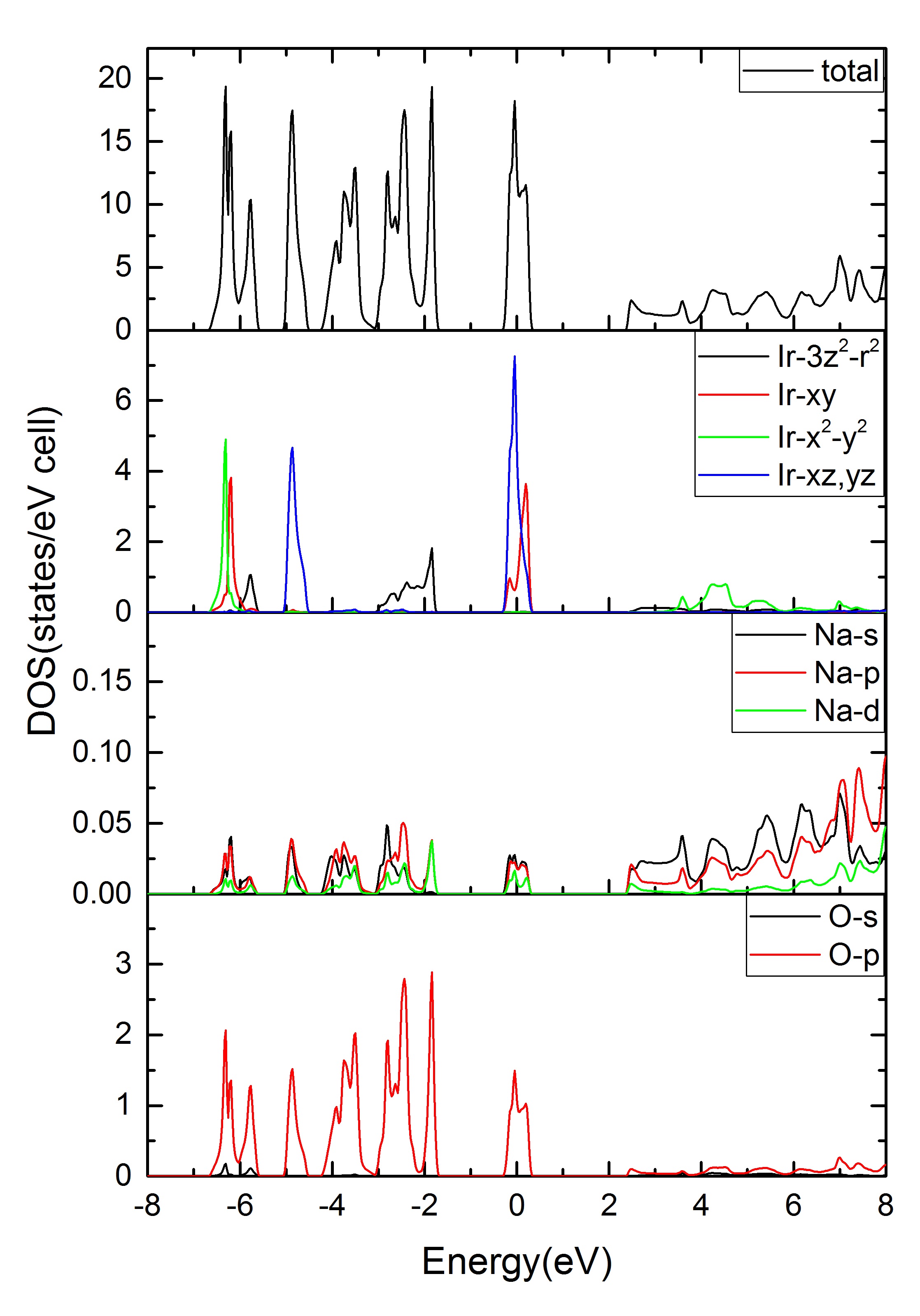
Figure 3: Partial density of states (PDOS) of Na₄IrO₄ calculated by the method of LDA calculation. The Fermi energy is set to zero.

To understand the magnetic properties, we also perform a spin polarized calculation and show the band structures of ferromagnetic (FM) configuration in Fig. 2(b) and 2(c). Basically, the $d_{3z^{2}-r^{2}}$ states are fully occupied while the $d_{x^{2}-y^{2}}$ ones are empty, and the spin polarization has a relatively small effect on these bands. On the other hand, the partially occupied $d_{xz}/d_{yz}$ and $d_{xy}$ states are significantly affected, and these bands have about 1 eV exchange splitting, as shown in Fig. 2(b) and 2(c). LSDA calculation for FM configuration gives a insulating solution with a band gap of 0.16 eV. Experiment reveals that Na₄IrO₄ has a long-range antiferromagnetic (AFM) order at low temperature 414 . Thus we also explore the magnetic configuration. In addition to the FM configuration, we also consider three AFM states: AFM-1 where Ir atoms at the body center and corners have opposite spin orientations, AFM-2 where Ir atoms couple anti-ferromagnetically along a-axis, AFM-3 where Ir atoms couple anti-ferromagnetically along c-axis (See Fig. 4 for the magnetic structures of different AFM configurations). The relative total energies and magnetic moments for the four magnetic configurations are summarized in Table. 1. Different magnetic configurations have similar calculated magnetic moments. This indicates that the magnetism in Na₄IrO₄ is quite localized. The distance between IrO₄ oxoanion is quite large as shown in Fig. 1, thus the effective hopping between Ir ions in Na₄IrO₄ is very weak. As a result, the magnetism in Na₄IrO₄ is very localized and different magnetic configurations have only small effects on the band structures. Regardless of the magnetic configuration, our numerical results show that the $5d$ electronic configuration can always be described by $d_{3z^{2}-r^{2},\uparrow}^{1}d_{3z^{2}-r^{2},\downarrow}^{1}d_{xz,\uparrow}^{1}d_{yz,\uparrow}^{1}d_{xy,\uparrow}^{1}$. While for most of $5d$ transition metal oxides, the magnetization is quite itinerant and the magnetic configuration strongly affect the band structure Rev-5d-3 . The calculated magnetic moment at Ir site is around 1.35 $\mu_{B}$, considerably small than that of $S$ = $3/2$ configuration. Due to the strong hybridization between Ir-$5d$ and O-$2p$ states, there is also considerable magnetic moment located at O site. As shown in Table 1, the AFM-1 configuration has the lowest total energy. Although we only consider four magnetic configurations, we believe that the AFM-1 is indeed the magnetic ground state configuration as discussed in the following sections.

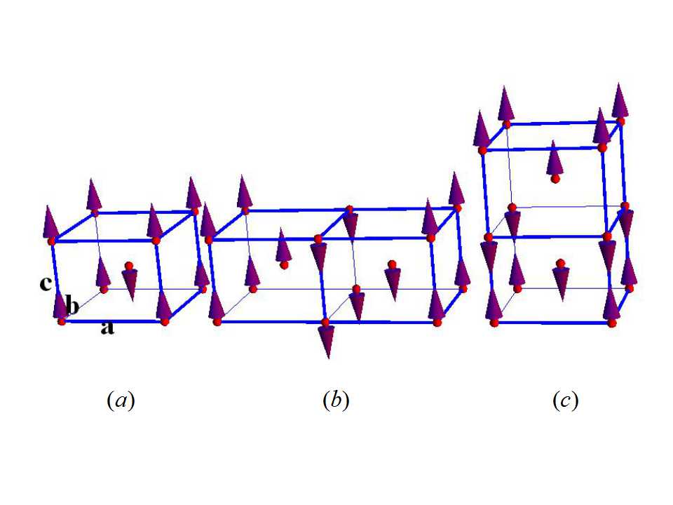
Figure 4: The AFM magnetic configurations of Na₄IrO₄ which we considered in DFT calculations. For clarity only Ir atoms are shown. (a), (b) and (c) represent AFM-1, AFM-2 and AFM-3 configurations, respecitvely.

Table 1: The calculated total energy (in meV) per unit cell and magnetic moments (in $\mu$B) for the four magnetic configurations from LSDA and LSDA + $U$ ($U$ = 2 eV) calculations. The total energy of AFM1 state is set to zero.

	LSDA				LSDA+$U$
	FM	AFM1	AFM2	AFM3	FM	AFM1	AFM2	AFM3
Etotal	44.5	0	19.7	17.9	22.8	0	10.8	8.4
mIr	1.40	1.32	1.34	1.35	1.48	1.45	1.46	1.46
mO	0.27	0.25	0.26	0.26	0.26	0.25	0.26	0.26

As the importance of electronic correlation for $5d$ orbitals has been recently emphasized Rev-5d-1 ; Rev-5d-2 ; Rev-5d-3 , we utilize the LSDA + $U$ scheme, which is adequate for the magnetically ordered insulating ground states, to consider the electronic correlation in Ir-$5d$ states. The estimates for the values of $U$ have been recently obtained between 1.4 and 2.4 eV in layered Sr₂IrO₄ and Ba₂IrO₄ 5dUvalue . The Ir ion in the IrO₄ moiety has only four nearest neighbors. Moreover IrO₄ moieties are highly-isolated, thus we generally expect that the value of $U$ in Na₄IrO₄ is larger than that in other $5d$ transition metal oxides. We have varied the value of $U$ from 2.0 to 3.0 eV, the electronic structure and magnetic properties depend moderately on $U$ and the numerical calculations show that the essential properties and our conclusions do not depend on the value of $U$. Thus we only show the results with $U$ = 2 eV at follows. Similarly we consider the four magnetic configurations and the results of relative total energies and magnetic moments are also summarized in Table. 1 while AFM-1 state still has the lowest energy. Including $U$ will enhance the exchange splitting in $5d$ bands, and slightly enlarge the calculated magnetic moments as shown in Table 1. The band structures of Na₄IrO₄ with AFM-1 order from the LSDA + $U$ calculation is presented in Fig. 5. The result from the LSDA calculation within the AFM-1 configuration is also shown for comparison. Compared with the LSDA calculation, the bands within LSDA + $U$ scheme are narrower but the order of crystal field splitting pattern and electronic occupation does not change. The LSDA + $U$ calculation predicts a little bigger magnetic moment for Ir ions (1.45 $\mu_{B}$) and a larger gap of about 0.57 eV, as shown in Table. 1 and Fig. 5. We also show the $d$ orbital splitting under the crystal field of square plane in the middle panel of Fig. 6, and the electronic occupation pattern is decided by the competition between the crystal field splitting and Hund’s rule. It is worth mentioning that the results such as the crystal splitting pattern, are not dependent on the value of $U$.

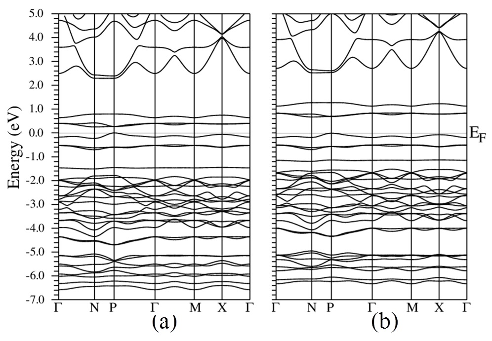
Figure 5: Band structure of AFM-1 configuration calculated by (a) LSDA (b) LSDA + $U$ (= 2 eV) method.

Figure 6: Schematic picture of orbital occupation around Fermi level. From LDA (left panel), LSDA+$U$ (middle panel) and LSDA+$U$+SOC (right panel) calculations. LSDA calculation has the same pattern with LSDA+$U$ calculations and is not presented here. $E_{F}$ represent the Fermi-level of Na₄IrO₄. As mentioned in the maintext, substituting Ir ions by Re ions, the Fermi-level shifts to $E_{F}^{\prime}$, which significantly enhances the MAE.

The strong SOC in $5d$ atoms usually significantly affects the band dispersions, thus we also perform the LSDA + $U$ + SOC calculations. Since the IrO₄ moiety is in the $ab$-plane, we perform the LSDA + $U$ + SOC calculations with spin orientations perpendicular to $ab$-plane and lying in $ab$-plane, i.e. the spin orientations are along (001), (010) and (100) directions. Our calculations show that the (001) is the easy axis and (100) is the hard axis. We list the calculated magnetic moments and total energies in Table 2 and find that AFM-1 state is still the ground state configuration. Unlike LSDA + $U$ calculations, the degeneracy of $d_{xz}$ and $d_{yz}$ is removed by SOC, as shown in Fig. 7 and the the right panel of Fig. 6. The most remarkable feature is the huge MAE. The MAE of Na₄IrO₄ is around 12 meV per Ir atom with the highly preferential easy axis being out of ab-plane. It is easy to see from Table. 2 that for all of the four magnetic configurations, (001) direction is the easy axis and the MAE have the similar values from 11.6 to 12.6 meV per Ir atom.

Large magnetic anisotropy energy (MAE) is desirable for magnetic devices. Recently, there has been considerable research interest in studying materials with a large MAE. Most of them are two dimensional materials or adatoms on surfaces. For example, Co atoms deposited on a Pt (111) surface pt , Fe or Mn atoms absorbed on the CuN surface cun , and Co or Fe atoms on Pd or Rh (111) surface pdrh . In addition, Rau et al. mgo found a giant MAE for the Co atoms absorbed on top of the O sites of MgO (001) surface. Generally, the bulk materials exhibit relatively small MAE of a few $\mu eV$ uev1 ; uev2 while anisotropy energies are larger by about three orders of magnitude for multilayers and surface systems uev2 . MAE originates from the interaction of the atom’s orbital magnetic moment and spin angular moment, thus an important factor of MAE is the strength of SOC, which increases from $3d$ to $5d$ metals. Another important factor is the special coordination environment, since a ligand field often quenches the orbital moment. Since the IrO₄ in Na₄IrO₄ shows an isolated planar structure, large MAE is expected.

In order to confirm the giant value of MAE, we also calculate the variation of the total energy by changing the magnetization direction with the force theorem. In this case, there is no need to converge a complete self-consistency cycle. The evaluated MAE using force theorem gives the similar values. We try to understand the magnetic properties in following sections.

Table 2: The calculated total energy (in meV) per unit cell and magnetic moments (in $\mu$B) for the four magnetic configurations from LSDA + SOC + $U$ ($U$ = 2 eV) calculations with (001) and (100) spin orientations. The total energy of AFM-1 state with (001) magnetization direction is set to zero. MAE (in meV) per Ir atom for four magnetic configurations are also summarized in the table.

	FM		AFM-1		AFM-2		AFM-3
	(001)	(100)	(001)	(100)	(001)	(100)	(001)	(100)
Etotal	22.3	34.4	0	11.6	11.1	22.8	8.9	21.5
mIr(spin)	1.37	1.38	1.34	1.35	1.36	1.36	1.36	1.36
mIr(orbital)	0.11	0.10	0.10	0.10	0.10	0.10	0.10	0.10
mO	0.25	0.24	0.24	0.23	0.24	0.24	0.24	0.24
MAE	12.1		11.6		11.7		12.6

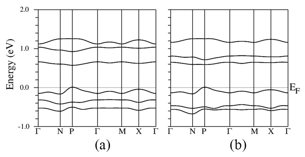
Figure 7: Band structure of Na₄IrO₄ calculated by the method of LSDA + $U$ + SOC ($U$ = 2 eV) calculation. (a) and (b) represent spin orientations along (001) direction and (100) direction, respectively.

IV Spin Model

As shown in Table 1, the calculated magnetic moments for the different magnetic configurations are similar, thus the total energy differences between the different magnetic configurations are mainly contributed by the inter-atomic exchange interaction where SOC is not considered. This allows us to estimate the exchange couplings by the energy-mapping analysis (see Appendix). As shown in Fig. 1, we consider three spin exchange paths. $J_{1}$ is the nearest-neighbor Ir-Ir exchange coupling along c-axis, $J_{2}$ is the next-nearest-neighbor one along diagonal line while $J_{3}$ is the 3rd-nearest-neighbor one along $a/b$-axis. The distance in $J_{3}$ (7.1 $\mathring{A}$) is much longer than $J_{1}$ (4.7 $\mathring{A}$) and $J_{2}$ (5.6 $\mathring{A}$). Compared with LSDA + $U$, LSDA overestimates the hopping, consequently gives larger exchange parameters as shown in Table 3. $J_{1}$, $J_{2}$ and $J_{3}$ are all AFM. Although $J_{1}$ has the nearest-neighbor exchange path, $d_{3z^{2}-r^{2}}$ orbital is fully occupied in both up and down spin channel as mentioned in the previous section and the hoppings for the other $d$ orbitals are relatively small. Therefore, it is easy to understand that the value of $J_{1}$ is less than $J_{2}$. Thus $J_{2}$ dominates over the others in strength, while $J_{3}$ is nearly negligible due to the much long distance, as shown in Table 3. Although the spin exchange couplings $J_{1}$-$J_{3}$ decrease with increasing $U$ values, $J_{2}$ is always dominated while $J_{3}$ is nearly negligible. The exchange interaction in magnetic insulators is predominantly caused by the so-called superexchange — which is due to the overlap of the localized orbitals of the magnetic electrons with those of intermediate ligands. The Ir-Ir distance in Na₄IrO₄ is very large, thus the value of exchange interaction $J$ with longer distance should be very smaller and have no influence on the magnetic ground state. Thus we believe that the strongest $J_{2}$ makes AFM-1 as the ground state, in agreement with the total energy calculations.

Based on the $J_{1}$-$J_{3}$ parameters from LSDA + $U$, we calculate the Curie-Weiss temperature $\theta$ and Néel temperature $T_{N}$ using the mean-field approximation theorytheta . $\theta$ is estimated to -105 K while $T_{N}$ is about 56 K. The values of -105 K and 56 K are both somewhat larger but qualitatively consistent with the experimental ones of -78 K and 25 K, respectively. Since the mean-field approximation theory often overestimate the Curie-Weiss and Néel temperatures, our mapping $J_{1}$-$J_{3}$ parameters are thought to be in reasonable agreement with experimental results.

V Magnetic anisotropy energy

In order to understand the origin of the giant MAE, we start from a generalized symmetry allowed spin model of Na₄IrO₄ (See Appendix):

$$H_{S}=-K\sum_{i}{S_{i}^{z}}^{2}+\frac{1}{2}\sum_{<i,j>,\alpha\beta}J_{ij}^{\alpha\beta}S_{i}^{\alpha}S_{j}^{\beta},$$ (1)

where the first term represents the single ion anisotropy Hamiltonian, the second one is the inter-atomic exchange Hamiltonian, $i,j$ label the Ir ions and $\alpha,\beta$ take $x,y,z$. Due to the inversion symmetry, $J_{ij}^{\alpha\beta}=J_{ij}^{\beta\alpha}$, which means there is no Dzyaloshinskii-Moriya interaction D ; M . We only consider the exchange neighbors $<ij>^{\prime}s$ to the 3rd nearest-neighbor, which are denoted by $J_{1},J_{2},J_{3}$ in order as shown in Fig. 1. For $J_{1}$, due to the $C_{4}$ rotation symmetry, $J_{1}^{\alpha\beta}=\delta_{\alpha\beta}J_{1}^{\alpha\alpha}$ and $J_{1}^{xx}=J_{1}^{yy}$. While for $J_{2}$ and $J_{3}$, the non-diagonal terms (i.e. $J^{xy},J^{xz}$ and $J^{yz}$) is symmetry-allowed, however these terms are proportional to the product of $\lambda^{2}$ and isotropic exchange nondiagonal , and should be very small, thus we ignore them hereafter.

Using the similar energy-mapping method (See Appendix), we estimate the parameters in Eq. (1) and show the results in Table. 3. It is clear that the anisotropy of spin exchange is small, especially for the dominating spin exchange, where $J_{2}$ shows a small difference between $J_{2}^{xx}$, $J_{2}^{yy}$ and $J_{2}^{zz}$. The different spin configurations have almost the same value of MAE, and the anisotropy of spin exchange coupling parameters is little, indicating that MAE is dominated by the single-ion anisotropy.

Table 3: Isotropic spin exchange parameters (in meV) and anisotropic spin exchange parameters evaluated by energy-mapping analysis from LSDA, LSDA + $U$, LSDA + SOC + $U$ ($U$ = 2 eV) calculations, respectively.

	LSDA	LSDA+$U$	LSDA+$U$+SOC
			$J_{i}^{xx}$	$J_{i}^{yy}$	$J_{i}^{zz}$
$J_{1}$/meV	0.97	0.66	0.32	0.32	0.51
$J_{2}$/meV	2.47	1.27	1.21	1.35	1.24
$J_{3}$/meV	0.56	0.14	0.02	0.02	0.01
$K$/meV	-	-	5.4

To understand the origin of single-ion anisotropy, we consider the crystal field splitting, electronic occupation shown in Fig. 6, and the SOC Hamiltonian $\lambda L\cdot S$ where $\lambda$ is the SOC constant. With the spin direction described by the two angles $(\theta,\varphi)$, where $\theta$ and $\varphi$ are the azimuthal and polar angles of the spin orientation with respect to the local coordinate environment, the $\lambda L\cdot S$ term can be written as soc

$$H_{so} =\lambda\hat{S}_{z^{\prime}}(\hat{L}_{z}\cos\theta+\frac{1}{2}\hat{L}_{+}e^{-i\varphi}\sin\theta+\frac{1}{2}\hat{L}_{-}e^{i\varphi}\sin\theta)$$

$$\quad+\frac{\lambda}{2}\hat{S}_{+^{\prime}}(-\hat{L}_{z}\sin\theta-\hat{L}_{+}e^{-i\varphi}\sin^{2}\frac{\theta}{2}+\hat{L}_{-}e^{i\varphi}\cos^{2}\frac{\theta}{2})$$

$$\quad+\frac{\lambda}{2}\hat{S}_{-^{\prime}}(-\hat{L}_{z}\sin\theta+\hat{L}_{+}e^{-i\varphi}\cos^{2}\frac{\theta}{2}+\hat{L}_{-}e^{i\varphi}\sin^{2}\frac{\theta}{2})$$ (2)

Using perturbation theory by treating the SOC Hamiltonian as the perturbation combined with the $d$ orbital occupation pattern, we can get the associated energy lowering:

$$\Delta E^{(1)} = \sum_{i}\left\langle i\left|H_{so}\right|i\right\rangle$$

$$\Delta E^{(2)} = -\sum\limits_{i,j}\frac{\left|\left\langle i\left|H_{so}\right|j\right\rangle\right|^{2}}{\left|e_{i}-e_{j}\right|}$$ (3)

where $i$ represents an occupied $d$-level state with energy $e_{i}$ while $j$ represents an unoccupied $d$-level state with energy $e_{j}$, and the third and higher order perturbations are not given here. In Na₄IrO₄, where the SOC has not been considered, $d_{xz,\uparrow}$ and $d_{yz,\uparrow}$ are doubly-degenerate. We can see that the degeneracy of $d_{xz,\uparrow}$ and $d_{yz,\uparrow}$ is lifted by the SOC and they split to $\left|Y_{2}^{1},\uparrow\right\rangle$ and $\left|Y_{2}^{-1},\uparrow\right\rangle$. The splitting is $\pm\frac{\lambda}{2}\left|\cos\theta\right|$ according to the first order perturbation, thus the splitting for the spin polarization of (001) direction is larger than that for (100) direction, as shown in Fig. 7. However, the $d_{xy,\uparrow}$, $d_{xz,\uparrow}$ and $d_{yz,\uparrow}$ are fully occupied and the band gap is quite big with respect to the SOC constant $\lambda$. Thus the first order perturbation is negligible and has no contribution to the single-ion anisotropy.

Therefore, we consider the second order perturbation. Note that in the common $5d$ transition metal oxides with face (or edge, corner)-sharing structure of oxygen octahedrons, the widths of the $t_{2g}$-block bandwidths are relatively large while the $\left|e_{i}-e_{j}\right|$ values are relatively small, so the perturbation theory does not lead to an accurate estimation of MAE. But in Na₄IrO₄, the widths of the bands around Fermi-level are about 0.2 eV and the $\left|e_{i}-e_{j}\right|$ value is around $\sim$2 eV, thus one can get the quantitative value of MAE more accurately by the second order perturbation

$$E=-\lambda^{2}\cos^{2}\theta[\frac{1}{4\Delta_{1}}+\frac{1}{4\Delta_{3}}-\frac{1}{2\Delta_{2}}]$$ (4)

Here $\Delta_{i}$ is the splitting of on-site $d$-orbital energy levels, as shown in Fig. 6. The orbitals of $d_{x^{2}-y^{2}}$ and $d_{z^{2}}$ are far away from the Fermi-level and can be ignored. From the LSDA + $U$ ($U$ = 2 eV) calculations, we estimate the orbital energy levels by the weight-center positions of DOS and get the values of $\Delta_{i}$. The calculated values of $\Delta_{1}$,$\ \Delta_{2}$ and $\Delta_{3}$ are 1.82, 1.35 and 0.89 eV, respectively. Using these value of $\Delta_{i}$ and $\lambda$ = 0.5 eV, we get the MAE as 12.0 meV, consistent with the value directly from DFT theory. Thus the second order perturbation is dominant in MAE and higher order perturbations are believed to be little. One reason of the giant MAE is the SOC strength, which is very strong for $5d$ electrons. It is about 3 times as high as $4d$ electrons and an order of magnitude higher than $3d$ electrons. Besides the strong SOC strength, the $d$-level splitting is also a significant cause of the giant MAE. The $d$-level splitting condition comes from the special square planar local environment which indicates a giant anisotropy between in-plane and out-of-plane. The long distances of IrO₄ moieties make the strong local magnetization. These factors together make the giant value of MAE.

We also calculate MAE with varying the SOC strength $\lambda$ within LSDA + $U$ + SOC scheme. As shown in Fig. 8, it is obviously that the MAE of Na₄IrO₄ is nearly proportional to the square of $\lambda$, in accordance with Eqn. (4).

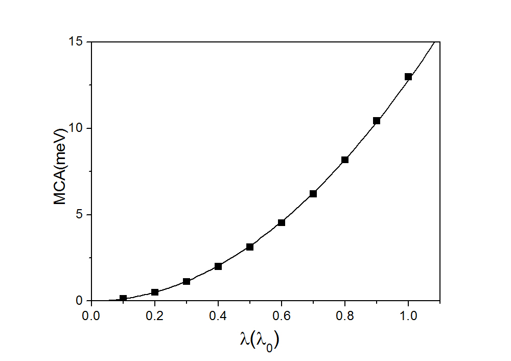
Figure 8: SOC strength dependence of the magnetic anisotropy energy of Na₄IrO₄ calculated by the method of LSDA + SOC + $U$ ($U$ = 2 eV).

Using the calculated spin model parameters, one can obtain the magnon spectrum on the basis of the Holstein-Prinmakoff transformation and the Fourier transformation. We calculate the spin-wave dispersion along high-symmetry axis and display the result in Fig. 9. As shown in Fig. 9, there is a large spin gap of about 26 meV while the width of spin-wave dispersion is only 4 meV. This is due to the large single-ion anisotropy and relatively small exchange couplings.

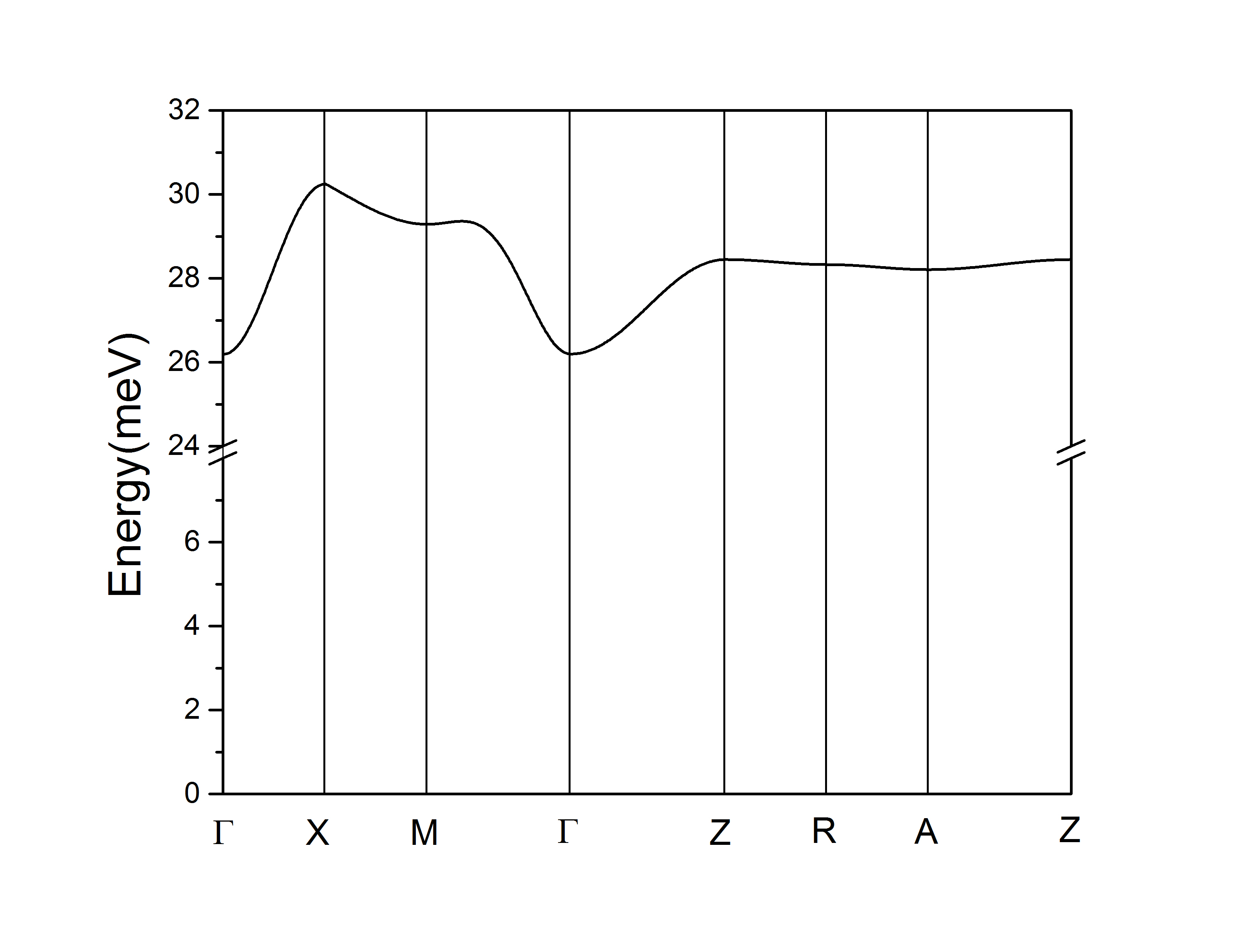
Figure 9: Calculated spin-wave dispersion curves along high-symmetry axis for the Na₄IrO₄.

VI Material Design

As shown in Fig. 6, for Na₄IrO₄, the exchange splitting is large and there is a relatively big gap between occupied and unoccupied states. Therefore the first order perturbation of SOC is very small. We expect that if the Fermi-level shifts to the position of $E_{F}^{\prime}$ as shown in Fig. 6, there is nonzero first order term and the MAE will be enhanced significantly. We try to realize the Fermi-level shift through substituting Ir ions in Na₄IrO₄ by Re ions. The MAE of Na₄ReO₄ may be even larger and it may reach the limit of MAE even in bulk materials, with the same size as Co or other atoms absorbed on top of the O sites of MgO (001) surface 3dmca ; wuhua .

In order to examine the dynamic stability, we calculate phonon spectrum of Na₄ReO₄ (See Appendix), and show the calculated phonon spectrum along high-symmetry lines in Fig. 10. All the phonon modes of Na₄ReO₄ are positive, indicating the structure is dynamically stable.

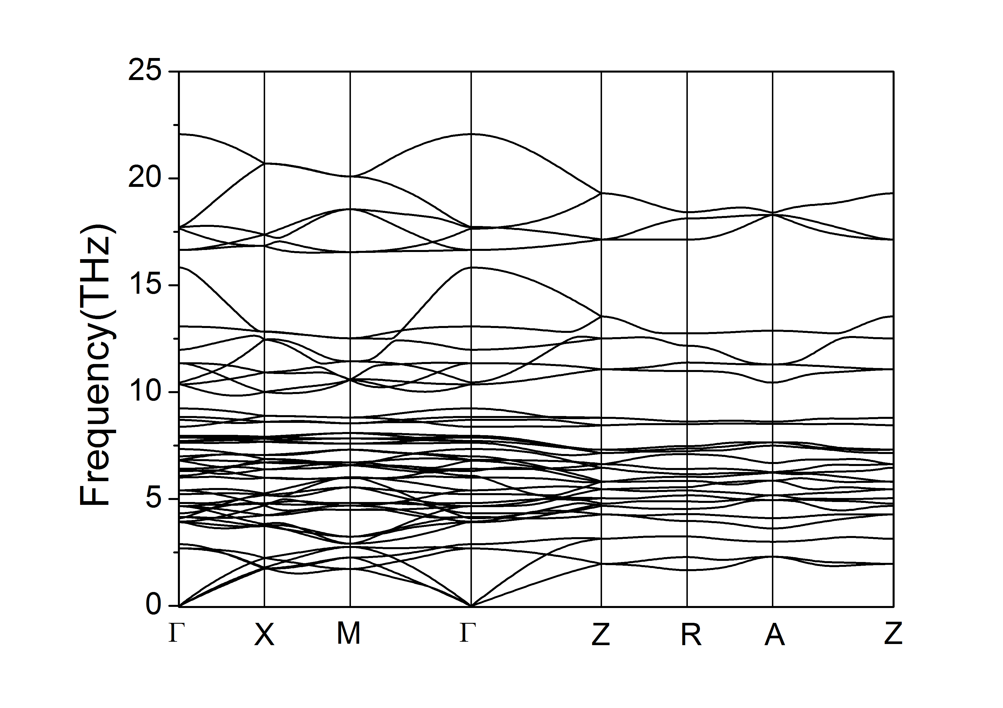
Figure 10: Calculated phonon dispersion for Na₄ReO₄.

The calculated value of MAE is about 140 meV per Ir atom. It can be explained by the same method using perturbation theory, where Na₄ReO₄ have two less occupied electrons. For Na₄ReO₄, with the absence of SOC interaction, the orbitals of $d_{xz,\uparrow}$ and $d_{yz,\uparrow}$ are doubly-degenerate and half-occupied. With the presence of SOC, the doubly-degenerate $d_{xz,\uparrow}$/$d_{yz,\uparrow}$ bands split to $\left|Y_{2}^{1},\uparrow\right\rangle$ and $\left|Y_{2}^{-1},\uparrow\right\rangle$, where $\left|Y_{2}^{-1},\uparrow\right\rangle$ is fully occupied while $\left|Y_{2}^{1},\uparrow\right\rangle$ is fully unoccupied. Thus the first order perturbation of total energy can be written as:

$$E=-\frac{\lambda}{2}\left|\cos\theta\right|$$ (5)

The calculated MAE of 140 meV is in good agreement with the expected value of $\frac{\lambda}{2}$, as the SOC strength $\lambda$ of the 5$d$ electrons is generally regarded as 0.3$\sim$0.5 eV.

VII Conclusions

In conclusion, using first-principles and perturbation theory, we present a comprehensive investigation of the $5d$ transition-metal oxides Na₄IrO₄, where Ir occupies the center of square-planar coordination environment. We discuss its electronic structures, determine its magnetic ground state configuration, and find a giant MAE for this compound. We clarify the microscopic mechanism about this novel magnetic properties, and also suggest possible way to further enhance MAE. We expect that the $5d$ transition metal oxides with low symmetry and long $5d$-$5d$ distance may exhibit extraordinarily large coercive fields. The prediction about giant MAE deserves experimental tests and may provide a route to nanoscale magnetic devices.

This work was supported by the Ministry of Science and Technology of China (Grant number: 2017YFA0303200), NSFC under Grants No. 11525417 and No. 11374137.

VIII Appendix

VIII.1 Symmetry analysis

Symmetry will add some restrictions on the magnetic model. Considering the time reversal symmetry and to the quadratic terms of spins, the magnetic model can be written in the following general form:

$$H=\frac{1}{2}\sum_{ls,l^{\prime}s^{\prime}}S_{ls}^{{\dagger}}J(ls,l^{\prime}s^{\prime})S_{l^{\prime}s^{\prime}},$$ (6)

where $S_{ls}$ represents the magnetic moment located at the magnetic ion labeled by $s$ in the $l$th unit cell. $J(ls,l^{\prime}s^{\prime})$ is the exchange interaction between $S_{ls}$ and $S_{l^{\prime}s^{\prime}}$. It is obviously a $3\times 3$ real matrix, because the magnetic moment is a three-component vector and we adopt the conventional Cartesian coordinate system. Translation symmetry will restrict $J(ls,l^{\prime}s^{\prime})$ to be related to $l^{\prime}-l$, irrespective of the starting unit cell. Rotation inversion or the combination of two will also give some restrictions on the exchange matrix. Considering a general space group element, $\{\alpha|\mathbf{t}\}$, of which $\alpha$ is the point operation, we denote the representation matrix as $R(\alpha)$ of $\alpha$ in the coordinate system here. Then $J(ls,l^{\prime}s^{\prime})$ should satisfy that,

$$R(\alpha)^{{\dagger}}J(mp,m^{\prime}p^{\prime})R(\alpha)=J(ls,l^{\prime}s^{\prime}),$$ (7)

where $mp$ and $m^{\prime}p^{\prime}$ are related to $ls$ and $l^{\prime}s^{\prime}$ by the action of $\{\alpha|\mathbf{t}\}$, respectively.

We then get ready to turn to the magnetic model for Na₄IrO₄. Because there is only one magnetic ion, namely Ir, in one unit cell, we can just label the magnetic moment by the unit cell label $l$. Utilizing the translation property, we just need to consider $J(0,l)$, which we denote to be $J(l)$ or $J(l_{1},l_{2},l_{3})$ hereafter. The onsite exchange $J(0,0,0)$ is found to own the following form,

$$J(0,0,0)=\left(\begin{array}[]{ccc}J(0,0,0)_{11}&0&0\\ 0&J(0,0,0)_{11}&0\\ 0&0&J(0,0,0)_{33}\end{array}\right),$$ (8)

which represent the single ion anisotropy $\sim S_{z}^{2}$.

According to the lattice parameters, we find that $l=(0,0,1)$ and $(0,0,-1)$ are for the nearest-neighborhoods, $l=(\eta_{1}1/2,\eta_{2}1/2,\eta_{3}1/2)$($\eta_{i}=\pm$) for the eight next-nearest-neighborhoods, and $l=(\pm 1,0,0),(0,\pm 1,0)$ for the 3rd-nearest-neighborhoods.

Then $J(0,0,\pm 1)$ are found to be in the following form:

$$J(0,0,\pm 1)=\left(\begin{array}[]{ccc}J(0,0,1)_{11}&0&0\\ 0&J(0,0,1)_{11}&0\\ 0&0&J(0,0,1)_{33}\end{array}\right),$$ (9)

and note that in the maintext, we relabel $J(0,0,1)_{11}$ and $J(0,0,1)_{22}$ to be $J_{1}^{xx}$ and $J_{1}^{yy}$, respectively.

For the next-nearest-neighborhoods, inversion symmetry will restrict $J(1/2,1/2,1/2)$ to be a symmetric matrix, which would allow finite non-diagonal elements. However we can ignore these symmetric non-diagonal elements, because physically they are relatively small nondiagonal . Then the $J(\eta_{1}1/2,\eta_{2}1/2,\eta_{3}1/2)$ are in the following form,

$$J(\eta_{1}1/2,\eta_{1}1/2,\pm 1/2)=\left(\begin{array}[]{ccc}J(1/2,1/2,1/2)_{11}&0&0\\ 0&J(1/2,1/2,1/2)_{22}&0\\ 0&0&J(1/2,1/2,1/2)_{33}\end{array}\right),$$ (10)

$$J(\eta_{1}1/2,-\eta_{1}1/2,\pm 1/2)=\left(\begin{array}[]{ccc}J(1/2,1/2,1/2)_{22}&0&0\\ 0&J(1/2,1/2,1/2)_{11}&0\\ 0&0&J(1/2,1/2,1/2)_{33}\end{array}\right),$$ (11)

and note that in the main text, we relabel $J(1/2,1/2,1/2)_{11}$, $J(1/2,1/2,1/2)_{22}$, and $J(1/2,1/2,1/2)_{33}$ to be $J_{2}^{xx}$, $J_{2}^{yy}$ and $J_{2}^{zz}$, respectively.

Finally $J(\pm 1,0,0)$ and $J(0,\pm 1,0)$ are found to be in the following form:

$$J(\pm 1,0,0)=\left(\begin{array}[]{ccc}J(1,0,0)_{11}&J(1,0,0)_{12}&0\\ J(1,0,0)_{12}&J(1,0,0)_{22}&0\\ 0&0&J(1,0,0)_{33}\end{array}\right),$$ (12)

$$J(0,\pm 1,0)=\left(\begin{array}[]{ccc}J(1,0,0)_{22}&-J(1,0,0)_{12}&0\\ -J(1,0,0)_{12}&J(1,0,0)_{11}&0\\ 0&0&J(1,0,0)_{33}\end{array}\right),$$ (13)

and note that in the main text, we relabel $J(1,0,0)_{11}$, $J(1,0,0)_{22}$ and $J(1,0,0)_{33}$ to be $J_{3}^{xx}$, $J_{3}^{yy}$ and $J_{3}^{zz}$, respectively. The non-diagonal elements $J(1,0,0)_{12}$ are still thought to be very small and ignored nondiagonal .

VIII.2 Energy-mapping analysis

We evaluate spin exchange parameters $J_{1}$-$J_{3}$ by energy-mapping analysis. Firstly we consider four magnetic configurations as shown in Fig. 4. The total energies of these four spin states can be described in terms of the spin Hamiltonian:

$$H=\sum_{i<j}J_{ij}\hat{S}_{i}\cdot\hat{S}_{j}$$ (14)

where $J_{ij}$ (= $J_{1}$, $J_{2}$, $J_{3}$) is the spin exchange parameter between the spin sites $i$ and $j$. By applying the energy expressions obtained for a spin dimer with S = 3/2 for Ir⁴⁺ ions, the total energies per unit cell for these four spin configurations are expressed as

$$E_{FM} =(2J_{1}+8J_{2}+4J_{3})(\frac{S^{2}}{2})$$ (15)

$$\quad E_{AFM1} =(2J_{1}-8J_{2}+4J_{3})(\frac{S^{2}}{2})$$ (16)

$$\quad E_{AFM2} =2J_{1}\times(\frac{S^{2}}{2})$$ (17)

$$\quad E_{AFM3} =(-\text{ }2J_{1}+4J_{3})(\frac{S^{2}}{2})$$ (18)

The relative energies of the four spin states are obtained from LSDA and LSDA + $U$ ($U$ = 2 eV) calculations and the values of $J_{1}$ to $J_{3}$ can be evaluated by mapping these energies. The calculated magnetic moments for the four magnetic configurations have little difference, as shown in Table. 1. The calculated spin exchange coupling parameters $J_{1}$ to $J_{3}$ are summarized in Table. 3. The spin exchanges $J_{1}$, $J_{2}$ and $J_{3}$ are all AFM and $J_{2}$ dominates over others in strength, while $J_{3}$ is almost negligible.

Considering a generalized symmetry allowed spin model described in Eq. (1), which includes the anisotropic part of $J$ and single-ion anisotropy, the values of $J^{xx}$, $J^{yy}$, $J^{zz}$ and $K$ can be determined by energy-mapping analysis of LSDA + $U$ + SOC calculations with different magnetization directions. In order to estimate these values, one more magnetic configuration should be considered, as shown in Fig. 11. The total energies per unit cell with different magnetic configurations are expressed as

$$E_{FM}^{(001)} =(2J_{1}^{zz}+8J_{2}^{zz}+4J_{3}^{zz})(\frac{S^{2}}{2})-KS^{2}$$ (19)

$$\quad E_{AFM1}^{(001)} =(2J_{1}^{zz}-8J_{2}^{zz}+4J_{3}^{zz})(\frac{S^{2}}{2})-KS^{2}$$ (20)

$$\quad E_{AFM2}^{(001)} =2J_{1}^{zz}\times(\frac{S^{2}}{2})-KS^{2}$$ (21)

$$\quad E_{AFM3}^{(001)} =(-\text{ }2J_{1}^{zz}+4J_{3}^{zz})(\frac{S^{2}}{2})-KS^{2}$$ (22)

$$E_{AFM4}^{(001)} =(2J_{1}^{zz}-4J_{3}^{zz})(\frac{S^{2}}{2})-KS^{2}$$ (23)

$$E_{FM}^{(100)} =(2J_{1}^{xx}+4J_{2}^{xx}+4J_{2}^{yy}+2J_{3}^{xx}+2J_{3}^{yy})(\frac{S^{2}}{2})$$ (24)

$$E_{AFM1}^{(100)} =(2J_{1}^{xx}-4J_{2}^{xx}-4J_{2}^{yy}+2J_{3}^{xx}+2J_{3}^{yy})(\frac{S^{2}}{2})$$ (25)

$$E_{AFM2}^{(100)} =(2J_{1}^{xx}+2J_{3}^{xx}-2J_{3}^{yy})(\frac{S^{2}}{2})$$ (26)

$$E_{AFM3}^{(100)} =(-2J_{1}^{xx}+2J_{3}^{xx}+2J_{3}^{yy})(\frac{S^{2}}{2})$$ (27)

$$E_{AFM4}^{(100)} =(2J_{1}^{xx}-4J_{2}^{xx}+4J_{2}^{yy}-2J_{3}^{xx}-2J_{3}^{yy})(\frac{S^{2}}{2})$$ (28)

$$E_{FM}^{(010)} =(2J_{1}^{xx}+4J_{2}^{xx}+4J_{2}^{yy}+2J_{3}^{xx}+2J_{3}^{yy})(\frac{S^{2}}{2})$$ (29)

$$E_{AFM1}^{(010)} =(2J_{1}^{xx}-4J_{2}^{xx}-4J_{2}^{yy}+2J_{3}^{xx}+2J_{3}^{yy})(\frac{S^{2}}{2})$$ (30)

$$E_{AFM2}^{(010)} =(2J_{1}^{xx}-2J_{3}^{xx}+2J_{3}^{yy})(\frac{S^{2}}{2})$$ (31)

$$E_{AFM3}^{(010)} =(-2J_{1}^{xx}+2J_{3}^{xx}+2J_{3}^{yy})(\frac{S^{2}}{2})$$ (32)

$$E_{AFM4}^{(010)} =(2J_{1}^{xx}+4J_{2}^{xx}-4J_{2}^{yy}-2J_{3}^{xx}-2J_{3}^{yy})(\frac{S^{2}}{2})$$ (33)

The relative total energies of these spin states are obtained from LSDA + $U$ + SOC calculations, which are summarized in Table. 4. The calculated magnetic moments for these magnetic configurations have little difference, as also summarized in Table. 4. By energy-mapping analysis, the calculated anisotropic spin exchange coupling parameters $J_{i}^{\alpha\alpha}$ and single-ion anisotropy parameter $K$ are summarized in Table. 3.

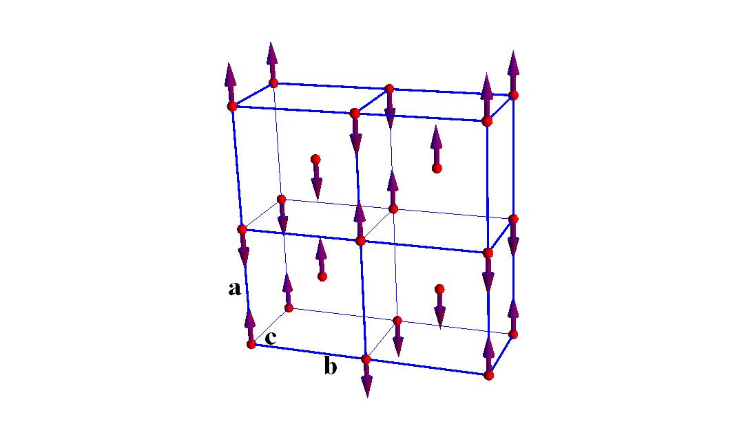
Figure 11: The AFM-4 magnetic configuration of Na₄IrO₄. For clarity only Ir atoms are shown.

Table 4: The calculated total energy (in meV) per unit cell and magnetic moments (in $\mu$B) for the four magnetic configurations from LSDA + SOC + $U$ ($U$ = 2 eV) calculations with (001), (010) and (100) spin orientations for energy-mapping analysis.

	FM			AFM-1			AFM-2			AFM-3			AFM-4
	(001)	(100)	(010)	(001)	(100)	(010)	(001)	(100)	(010)	(001)	(100)	(010)	(001)	(100)	(010)
Etotal	22.3	34.4	34.4	0	11.6	11.6	11.1	22.8	22.8	8.9	21.5	21.5	10.9	23.3	21.7
mIr(spin)	1.37	1.38	1.38	1.34	1.35	1.35	1.36	1.36	1.36	1.36	1.36	1.36	1.36	1.36	1.36
mIr(orbital)	0.11	0.10	0.10	0.10	0.10	0.10	0.10	0.10	0.10	0.10	0.10	0.10	0.10	0.10	0.10
mO	0.25	0.24	0.24	0.24	0.23	0.23	0.24	0.24	0.24	0.24	0.24	0.24	0.24	0.24	0.24

VIII.3 Details of results for Na₄ReO₄

The phonon calculation is performed from the finite displacement method as implemented in the Vienna ab-initio simulation package (VASP) vasp1 ; vasp2 ; vasp3 and the PHONOPY package vasp4 . After a series of tests, a $3\times 3\times 2$ supercell is constructed to ensure the force convergence, and a $2\times 2\times 4$ k-mesh for the Brillouin zone sampling is used in the phonon calculation. The calculated phonon spectrum along high-symmetry lines is shown in Fig. 10.

In Na₄ReO₄ case, Re⁴⁺ ion has two less occupied $5d$ electrons than Ir⁴⁺ ion. We perform first-principles calculations and find that the crystal field splitting does not change. The calculated magnetic moment is 0.51 $\mu_{B}$. We perform several calculations for different magnetic configurations and find that the magnetic ground-state configuration is the FM state. The calculated spin exchange coupling parameters $J_{1}$ to $J_{3}$ are -1.84 meV, -0.84 meV and -0.04 meV, respectively. However, the single-ion anisotropy has a overwhelmingly major contribution on MAE especially in Na₄ReO₄, which has an order of magnitude larger single-ion anisotropy than Na₄IrO₄.

References

- (1) M. Imada, A. Fujimori, and Y. Tokura, Rev. Mod. Phys. 70, 1039 (1998).
- (2) G. Kotliar, S. Y. Savrasov, K. Haule, V. S. Oudovenko, O. Parcollet, and C. A. Marianetti, Rev. Mod. Phys. 78, 865 (2006).
- (3) W. Witczak-Krempa, G. Chen, Y. B. Kim, and L. Balents, Annu. Rev. Condensed Matter Physics 5, 57 (2013).
- (4) J. G. Rau, E. K.-H. Lee, and H.-Y. Kee, Annu. Rev. Condensed Matter Physics 7, 195 (2016).
- (5) Y. Du and X. Wan, Computational Mater. Sci. 112, 416 (2016).
- (6) B. J. Kim et al., Phys. Rev. Lett. 101, 076402 (2008); B. J. Kim et al., Science 323, 1329 (2009).
- (7) H. Jin, H. Jeong, T. Ozaki, J. Yu, Phys. Rev. B 80, 075112 (2009).
- (8) H. Watanabe, T. Shirakawa, S. Yunoki, Phys. Rev. Lett. 105, 216410 (2010).
- (9) A. Shitade, H. Katsura, J. Kuneš, X.-L. Qi, S.-C. Zhang, N. Nagaosa, Phys. Rev. Lett. 102, 256403 (2009).
- (10) D.A. Pesin, L. Balents, Nat. Phys. 6, 376 (2010).
- (11) C. H. Kim, H. S. Kim, H. Jeong, H. Jin, and J. Yu, Phys. Rev. Lett. 108, 106401 (2012).
- (12) G. Jackeli, G. Khaliulin, Phys. Rev. Lett. 102, 017205 (2009); J. Chaloupka, G. Jackeli, and G. Khaliullin, Phys. Rev. Lett. 105, 027204 (2010).
- (13) X. Wan, A. M. Turner, A. Vishwanath, and S. Y. Savrasov, Phys. Rev. B 83, 205101 (2011).
- (14) F. Wang, T. Senthil, Phys. Rev. Lett. 106, 136402 (2011).
- (15) X. Wan, A. Vishwanath, S.Y. Savrasov, Phys. Rev. Lett. 108, 146601 (2012).
- (16) T. Okamoto, M. Nohara, H. Aruga-Katori, H. Takagi, Phys. Rev. Lett. 99, 137207 (2007).
- (17) P.A. Lee, Science 321, 1306 (2008); L. Balents, Nature 464, 199 (2010).
- (18) D. Mandrus, J. R. Thompson, R. Gaal, L. Forro, J. C. Bryan, B. C. Chakoumakos, L. M. Woods, B. C. Sales, R. S. Fishman, and V. Keppens, Phys. Rev. B 63, 195104 (2001); W. J. Padilla, D. Mandrus, and D. N. Basov, Phys. Rev. B 66, 035120 (2002).
- (19) Y. G. Shi, Y. F. Guo, S. Yu, M. Arai, A. A. Belik, A. Sato, K. Yamaura, E. Takayama-Muromachi, H. F. Tian, H. X. Yang, J. Q. Li, T. Varga, J. F. Mitchell, and S. Okamoto, Phys. Rev. B 80, 161104 (2009).
- (20) Y. Du, X. Wan, L. Sheng, J. Dong, and S. Y. Savrasov, 85, 174424 (2012); M.-C. Jung, Y.-J. Song, K.-W. Lee, and W. E. Pickett, Phys. Rev. B 87, 115119 (2013).
- (21) Y. Shi, Y. Guo, X.Wang, A. J. Princep, D. Khalyavin, P.Manuel, Y. Michiue, A. Sato, K. Tsuda, S. Yu, M. Arai, Y. Shirako, M. Akaogi, N. Wang, K. Yamaura, and A. T. Boothroyd, Nature Mat. 12, 1024 (2013).
- (22) H. Sim and B. G. Kim, Phys. Rev. B 89, 201107(R) (2014); H. J. Xiang, Phys. Rev. B 90, 094108 (2014); H. M. Liu, Y. P. Du, Y. L. Xie, J.-M. Liu, C.-G. Duan, and X. Wan, Phys. Rev. B 91, 064104 (2015).
- (23) R. Comin, G. Levy, B. Ludbrook, Z.-H. Zhu, C. N. Veenstra, J. A. Rosen, Y. Singh, P. Gegenwart, D. Stricker, J. N. Hancock, D. van der Marel, I. S. Elfimov, and A. Damascelli, Phys. Rev. Lett. 109, 266406 (2012).
- (24) K.Mader, R. Hoppe, Z. Anorg. Allg. Chem. 619, 1647 (1993).
- (25) S. Kanungo, B. Yan, P. Merz, C. Felser, and M. Jansen, Angew. Chem. 127, 5507 (2015).
- (26) P. Blaha, K. Schwarz, G. K. H. Madsen, D. Kvasnicka, and J. Luitz, WIEN2K, An Augmented Plane Wave+ Local Orbitals Program for Calculating Crystal Properties (Karlheinz Schwarz, Technische Universität Wien, Austria, 2001).
- (27) J. Kuneš, T. Jeong, and W. E. Pickett, Phys. Rev. B 70, 174510 (2004); D. J. Singh, J. Appl. Phys. 79, 4818 (1996); A. T. Zayak, X. Huang, J. B. Neaton, and K. M. Rabe, Phys. Rev. B 77, 214410 (2008); X. Wan, J. Zhou, and J. Dong, Europhys. Lett. 92, 57007 (2010).
- (28) D. D. Koelling and B. N. Harmon, J. Phys. C 10, 3107 (1977).
- (29) V. I. Anisimov, F. Aryasetiawan, and A. I. Lichtenstein, J. Phys. Condens. Matter 9, 767 (1997).
- (30) B. J. Kim, H. Ohsumi, T. Komesu, S. Sakai, T. Morita, H. Takagi, and T. Arima, Science 323, 1329 (2009).
- (31) R. Arita, J. Kuneš, A.V. Kozhevnikov, A.G. Eguiluz, and M. Imada, Phys. Rev. Lett. 108, 086403 (2012).
- (32) G. Kresse and J. Furthmüller, Comput. Mater. Sci. 6, 15 (1996).
- (33) G. Kresse and J. Furthmüller, Phys. Rev. B 54, 11169 (1996).
- (34) G. Kresse and D. Joubert, Phys. Rev. B 59, 1758 (1999).
- (35) A. Togo, F. Oba and I. Tanaka, Phys. Rev. B 78, 134106 (2008).
- (36) I. G. Rau, S. Baumann, S. Rusponi, F. Donati, S. Stepanow, L. Gragnaniello, J. Dreiser, C. Piamonteze, F. Nolting, S.Gangopadhyay, O. R. Albertini, R.M. Macfarlane, C. P. Lutz, B. A. Jones, P. Gambardella, A. J. Heinrich, and H. Brune, Science 344, 988 (2014).
- (37) X. Ou, H. Wang, F. Fan, Z. Li, and H. Wu, Phys. Rev. Lett. 115, 257201 (2015).
- (38) P. Gambardella, S. Rusponi, M. Veronese, S. S. Dhesi, C. Grazioli, A. Dallmeyer, I. Cabria, R. Zeller, P. H. Dederichs, K. Kern, C. Carbone, and H. Brune, Science 300, 1130 (2003).
- (39) C. F. Hirjibehedin, C. Y. Lin, A. F. Otte, M. Ternes, C. P. Lutz, B. A. Jones, and A. J. Heinrich, Science 317, 1199 (2007).
- (40) P. Blonski, A. Lehnert, S. Dennler, S. Rusponi, M. Etzkorn, G. Moulas, P. Bencok, P. Gambardella, H. Brune, and J. Hafner, Phys. Rev. B 81, 104426 (2010).
- (41) I. G. Rau, S. Baumann, S. Rusponi, F. Donati, S. Stepanow, L. Gragnaniello, J. Dreiser, C. Piamonteze, F. Nolting, S. Gangopadhyay, O. R. Albertini, R.M. Macfarlane, C. P. Lutz, B. A. Jones, P. Gambardella, A. J. Heinrich, and H. Brune, Science 344, 988 (2014).
- (42) G. H. O. Daalderop, P. J. Kelly, and M. F. H. Schuurmans, Phys. Rev. B 41, 11919 (1990).
- (43) R. Wu and A. J. Freeman, J. Magn. Magn. Mater. 200, 498 (1999).
- (44) J. Samuel Smart, Effective Field Theories of Magnetism (W. B. Sauders Company, 1966).
- (45) I. Dzyaloshinskii, Journal of Physics and Chemistry of Solids 4, 241 (1958).
- (46) T. Moria, Physical Review 120, 91 (1960).
- (47) M-H Whangbo, H-J Koo, and Dadi Dai, Journal of Solid State Chemistry 176, 417 (2003).
- (48) D. Dai, H. J. Xiang, and M.-H. Whangbo, J. Comput. Chem. 29, 13 (2008).