Asymptotic formula of the number of Newton polygons

Abstract

In this paper, we enumerate Newton polygons asymptotically. The number of Newton polygons is computable by a simple recurrence equation, but unexpectedly the asymptotic formula of its logarithm contains growing oscillatory terms. As the terms come from non-trivial zeros of the Riemann zeta function, an estimation of the amplitude of the oscillating part is equivalent to the Riemann hypothesis.

Keywords: Newton polygons, Asymptotic formula, Riemann hypothesis, Central limit theorem

2010 Mathematical Subject Classification: 11P82, 11M06

1 Introduction

In many algebro-geometric contexts, Newton polygons appear as combinatorial invariants of algebraic objects. For instance, a polynomial over a local field defines a Newton polygon, which knows much about how the polynomial factors. It is also well-known as Dieudonné-Manin classification (cf. [7]) that isogeny classes of $p$-divisible groups (resp. the $p$-divisible groups of abelian varieties) over an algebraically closed field in characteristic $p>0$ are classified by Newton polygons (resp. symmetric Newton polygons), where $p$-divisible groups are also called Barsotti-Tate groups. Also similar combinatorial data appear when we consider the Harder-Narasimhan filtration of vector bundles (cf. [5]). This paper aims to show that Newton polygons are not only useful to study such algebraic objects but also have an importance on the number of them.

A Newton polygon of height $n$ is a lower convex line graph $\xi$ over the interval $[0,n]$ with $\xi(0)=0$ where all breaking points of $\xi$ belong to ${\mathbb{Z}}^{2}$. Our main theorem (Theorem 3.1.1) describes the asymptotic behavior of the number ${\mathcal{N}}(n)$ of Newton polygons of height $n$ with slopes $\in[0,1)$ as $n\to\infty$. It says that the logarithm of ${\mathcal{N}}(n)$ oscillates around the logarithm of

$${\mathcal{P}}(n):=\frac{C^{1/9}K}{\sqrt{6\pi}}\frac{1}{n^{11/18}}\exp\left(\frac{3}{2}C^{1/3}n^{2/3}\right),$$

where $C=2\zeta(3)/\zeta(2)=1.4615\cdots$ and $K=\exp(-2\zeta^{\prime}(-1)-\log(2\pi)/6)=1.0248\cdots$. The oscillating terms are the second main terms but the coefficients of the terms are so small that it would be hard to predict the oscillation from any computational enumeration from the definition of ${\mathcal{N}}(n)$, whereas the value of the constant $C^{1/9}K/\sqrt{6\pi}$ could be approximately predicted. The oscillation gets larger and larger as $n$ increases. We shall see in Theorem 3.1.2 that the amplitude of the oscillating part of the logarithm of ${\mathcal{N}}(n)$ is $O(n^{1/6+\epsilon})$ for any $\epsilon>0$ if the Riemann hypothesis (cf. [9] and [10, 10.1]) is true and has a larger order otherwise.

This paper is organized as follows. In Section 2, we find a generating function of ${\mathcal{N}}(n)$ and describe the logarithm of the generating function. Section 3 is the main part of this paper. Our main results are stated in Section 3.1. In Section 3.2, we give a proof of the asymptotic formula (Theorem 3.1.1), following the method of the paper [1] by Báez-Duarte, where Hardy-Ramanujan asymptotic formula [6] for partitions of integers was re-proved by applying Lyapunov’s central limit theorem with some tail estimations. In Section 3.3 we prove the second theorem (Theorem 3.1.2) on the relation between the amplitude of the oscillation and the Riemann hypothesis. In Section 3.4, we treat two variants: one is the case that slopes belong to the interval $[0,1]$ and the other is the case that Newton polygons are symmetric. In Section 4 we find a recurrence equation for the numbers of Newton polygons and observe the asymptotic formula with numerical data.

Acknowledgments

This work started with the graduation thesis (February in 2017) by Takuya Tani (supervised by the author), where a variant of the generating function (2) was found. I would like to thank Professor Norio Konno for helpful suggestions and supports continuing after Tani’s presentation of his graduation thesis, which led me to the probabilistic approach. The author also thank the anonymous referee for his/her careful reading and helpful comments. This work was supported by JSPS Grant-in-Aid for Scientific Research (C) 17K05196.

2 The generating function and its logarithm

In this section, we find a generating function for the numbers of Newton polygons, and study its logarithm.

2.1 The generating function

A Newton polygon of height $n$ and depth $d$ is a lower convex line graph starting at $(0,0)$ and ending at $(n,d)$ with breaking points belonging to ${\mathbb{Z}}^{2}$. Let $n$ and $d$ be non-negative integers. Let $\rho(n,d)$ be the number of Newton polygons of height $n$ and depth $d$ with non-negative slopes $<1$. Note

$${\mathcal{N}}(n)=\sum_{d=0}^{\infty}\rho(n,d)$$ (1)

with $\rho(n,d)=0$ for $d\geq\max\{1,n\}$.

A Newton polygon is expressed as a multiple set of segments, where a segment is a pair $(k,\ell)$ of non-negative integers $k,\ell$ with $\gcd(k,\ell)=1$. Indeed, for a multiple set $\xi:=\{(k_{i},\ell_{i})\mid i=1,2,\ldots,t\}$ of segments with $n=\sum k_{i}$ and $d=\sum\ell_{i}$, we arrange them so that $\ell_{i}/k_{i}\leq\ell_{j}/k_{j}$ for $i<j$, and to $\xi$ we associate the Newton polygon of Figure 1.

Figure 1: Newton polygon

We have a generating function of $\rho(n,d)$ in the following form

$$\prod_{\begin{matrix}0\leq\ell/k<1,\\ \gcd(k,\ell)=1\end{matrix}}\frac{1}{1-x^{k}y^{\ell}}=\sum_{n=0}^{\infty}\sum_{d=0}^{n}\rho(n,d)x^{n}y^{d}.$$ (2)

To see this equation, we compare the $x^{n}y^{d}$-coefficients of the both sides. The $x^{n}y^{d}$-coefficient of the left-hand side is the number of multiple sets $\{(k_{i},\ell_{i})\}$ with $0\leq\ell_{i}/k_{i}<1$ and $\gcd(k_{i},\ell_{i})=1$ such that $\sum k_{i}=n$ and $\sum\ell_{i}=d$, which is nothing other than $\rho(n,d)$.

Substituting $1$ for $y$, we get

$$f(x):=\prod_{k=1}^{\infty}\left(\frac{1}{1-x^{k}}\right)^{\varphi(k)}=\sum_{n=0}^{\infty}{\mathcal{N}}(n)x^{n},$$ (3)

where $\varphi(k)$ is Euler’s totient function. The radius of convergence of $f(x)$ is one, since

$$\sum_{k=1}^{\infty}\varphi(k)\left|\frac{x^{k}}{1-x^{k}}\right|<\frac{1}{1-|x|}\sum_{k=1}^{\infty}k|x|^{k}<\infty$$ (4)

for any $|x|<1$.

2.2 The logarithm of the generating function

We study the logarithm of $f(e^{-\tau})$ for ${\operatorname{Re}}(\tau)>0$, following the method of Meinardus [8]. First we expand it as

$$\log f(e^{-\tau})=\sum_{k=1}^{\infty}\varphi(k)\sum_{m=1}^{\infty}\frac{1}{m}e^{-mk\tau}.$$

By the formula of Cahen and Mellin

$$e^{-\tau}=\frac{1}{2\pi i}\int_{\sigma_{0}-i\infty}^{\sigma_{0}+i\infty}\Gamma(s)\frac{1}{\tau^{s}}\ ds\quad({\operatorname{Re}}(\tau)>0,\sigma_{0}>0),$$

we get

$$\log f(e^{-\tau}) = \frac{1}{2\pi i}\int_{\sigma_{0}-i\infty}^{\sigma_{0}+i\infty}\frac{1}{\tau^{s}}\Gamma(s)\sum_{m=1}^{\infty}\frac{1}{m^{s+1}}\sum_{k=1}^{\infty}\frac{\varphi(k)}{k^{s}}\ ds$$ (5)

$$= \frac{1}{2\pi i}\int_{\sigma_{0}-i\infty}^{\sigma_{0}+i\infty}\frac{1}{\tau^{s}}\Gamma(s)\zeta(s+1)\frac{\zeta(s-1)}{\zeta(s)}\ ds$$

for $\sigma_{0}>2$. A formula of $\log f(e^{-\tau})$ will be obtained by moving the line of integration to the left.

Recall the fact [10, Theorem 9.7] that there exists a constant $A$ such that for every $\nu$ there exists $t_{\nu}\in[\nu,\nu+1]$ for which

$$\left|\frac{1}{\zeta(\sigma+it_{\nu})}\right|\leq t_{\nu}^{A}\quad(-1\leq\sigma\leq 2).$$ (6)

It is obvious to extend the interval to an arbitrary interval by using the well-known order-estimations as $|t|\to\infty$: $|\zeta^{\pm 1}(\sigma+it)|=O(1)$ for $\sigma>1$ (cf. [10, 3.1]) and $|\zeta^{\pm 1}(\sigma+it)|=O\left(|t|^{-\sigma+1/2}\right)$ for $\sigma<0$ (cf. [10, (4.12.3)]. Also it is known that $|\zeta^{\pm 1}(1+it)|=O(|t|^{\epsilon})$ for any $\epsilon>0$ (cf. [10, (3.5.2), (3.6.5)]). As for the estimation of $\zeta(s)$ in the critical strip, for instance use the convexity bound $|\zeta(s)|=O\left(|t|^{(1-\sigma)/2+\epsilon}\right)$ for any $\epsilon>0$, see [10, 5.1]. From Stirling’s formula (cf. [10, (4.12.2)]), in an arbitrary strip $a\leq{\operatorname{Re}}(s)\leq b$, for any $\varepsilon>0$ we have

$$\Gamma(s)=O\left(e^{-(\pi/2-\varepsilon)|{\operatorname{Im}}(s)|}\right)$$ (7)

as $|{\operatorname{Im}}(s)|\to\infty$, and $\Gamma(s)$ is rapidly decreasing also as $\sigma\to-\infty$.

Let $S$ be the set of poles of $\tau^{-s}\Gamma(s)\zeta(s+1)\zeta(s-1)\zeta(s)^{-1}$, and $g_{\alpha}(\tau)$ its residue at $\alpha\in S$:

$$g_{\alpha}(\tau):=\operatorname{Res}_{s=\alpha}\left(\tau^{-s}\Gamma(s)\zeta(s+1)\frac{\zeta(s-1)}{\zeta(s)}\right).$$ (8)

It is known that $\Gamma(s)$ has no zero and has poles only at non-positive integers and the poles are all simple. Note that $S$ consists of $2,0$ and the (non-trivial and trivial=negative even) zeros of $\zeta(s)$. Let $c_{0}$ be a real number with $c_{0}\geq 1$ or $c_{0}<0$, and assume that $c_{0}$ is not equal to the real part of any element $\alpha$ of $S$. Then $\log f(e^{-\tau})$ is equal to

$$\sum_{\alpha\in S\text{ s.t. }{\operatorname{Re}}(\alpha)>c_{0}}g_{\alpha}(\tau)+\frac{1}{2\pi i}\int_{c_{0}-i\infty}^{c_{0}+i\infty}\frac{1}{\tau^{s}}\Gamma(s)\zeta(s+1)\frac{\zeta(s-1)}{\zeta(s)}\ ds,$$ (9)

where for $c_{0}<0$ the sum is precisely

$$\lim_{\nu\to\infty}\sum_{\begin{matrix}\alpha\in S\text{ s.t. }{\operatorname{Re}}(\alpha)>c_{0},\\ |{\operatorname{Im}}(\alpha)|<t_{\nu}\end{matrix}}g_{\alpha}(\tau)$$ (10)

with $t_{\nu}$ as in (6) and this converges. As the integral in (9) is $O(|\tau|^{-c_{0}})$ by (7) with the other order-estimations reviewed above, we obtain

$$\log f(e^{-\tau})=\sum_{\alpha\in S\text{ s.t. }{\operatorname{Re}}(\alpha)>c_{0}}g_{\alpha}(\tau)+O(|\tau|^{-c_{0}}).$$ (11)

The residue of each pole is as follows. First the residue at $s=2$ is

$$g_{2}(\tau)=\frac{\zeta(3)}{\zeta(2)}\cdot\frac{1}{\tau^{2}}.$$ (12)

Let $\gamma$ be a non-trivial zero of $\zeta(s)$. If $\gamma$ is a simple zero, then

$$g_{\gamma}(\tau)=\frac{\Gamma(\gamma)\zeta(\gamma+1)\zeta(\gamma-1)}{\zeta^{\prime}(\gamma)}\cdot\frac{1}{\tau^{\gamma}}.$$ (13)

In general, $g_{\gamma}(\tau)$ is of the form

$$g_{\gamma}(\tau)=\tau^{-\gamma}P_{\gamma}(\log\tau)$$

for some polynomial $P_{\gamma}$ whose degree is the order at $\gamma$ of $\zeta(s)$ minus $1$.

The order of the pole at $s=0$ of $\Gamma(s)\zeta(s+1)\zeta(s-1)\zeta(s)^{-1}$ is two. We have $g_{0}(\tau)=D^{\prime}(0)-D(0)\log\tau$ with $D(s)=\zeta(s-1)/\zeta(s)$, whence

$$g_{0}(\tau)=-\frac{1}{6}\log\tau-2\zeta^{\prime}(-1)-\frac{1}{6}\log(2\pi).$$ (14)

We forgo determining $g_{\alpha}(\tau)$ for ${\operatorname{Re}}(\alpha)\leq-2$, as those contributions to our asymptotic formula are much smaller than the errors appearing in Section 3.2.

Proposition 2.2.1.

For any $\epsilon>0$, we have

$$\log f(e^{-\tau}) = \frac{\zeta(3)}{\zeta(2)}\tau^{-2}+\sum_{\gamma}g_{\gamma}(\tau)-\frac{1}{6}\log\tau-2\zeta^{\prime}(-1)-\frac{1}{6}\log(2\pi)+O(|\tau|^{2-\epsilon})$$

$$= \frac{\zeta(3)}{\zeta(2)}\tau^{-2}+O(\tau^{-1}).$$

as $\tau\to 0$, where $\gamma$ runs through non-trivial zeros of $\zeta(s)$.

Proof.

The first equality follows from (11) for $c_{0}=-2+\epsilon$ with (12) and (14). The second one follows from (11) for $c_{0}=1$. ∎

Remark 2.2.2.

In the same way, for any natural number $\nu$, one can show

$$\left(-\frac{d}{d\tau}\right)^{\nu}\log(e^{-\tau}) = (\nu+1)!\frac{\zeta(3)}{\zeta(2)}\frac{1}{\tau^{\nu+2}}+(-1)^{\nu}\sum_{\gamma}g_{\gamma}^{(\nu)}(\tau)$$

$$+\frac{(\nu-1)!}{6}\frac{1}{\tau^{\nu}}+O(|\tau|^{2-\nu-\epsilon})$$

$$= (\nu+1)!\frac{\zeta(3)}{\zeta(2)}\frac{1}{\tau^{\nu+2}}+O(\tau^{-1-\nu})$$

for any $\epsilon>0$, from the $\nu$-th derivative of (5)

$$\left(-\frac{d}{d\tau}\right)^{\nu}\log f(e^{-\tau})=\frac{1}{2\pi i}\int_{\sigma_{0}-i\infty}^{\sigma_{0}+i\infty}\frac{1}{\tau^{s+\nu}}\Gamma(s+\nu)\zeta(s+1)\frac{\zeta(s-1)}{\zeta(s)}\ ds$$

for $\sigma_{0}>2$.

3 The asymptotic formula

We state the main results on the asymptotic formula of ${\mathcal{N}}(n)$ and on relations to the Riemann hypothesis in Section 3.1, and prove them in later subsections.

3.1 Main results

Here is the main result on the asymptotic formula of ${\mathcal{N}}(n)$.

Theorem 3.1.1.

We have

$${\mathcal{N}}(n)\sim\frac{C^{1/9}K}{\sqrt{6\pi}}\frac{1}{n^{11/18}}\exp\left(\frac{3}{2}C^{1/3}n^{2/3}+\sum_{\gamma}g_{\gamma}\left(C^{1/3}n^{-1/3}\right)\right)$$

with $\displaystyle C=2\frac{\zeta(3)}{\zeta(2)}$ and $\displaystyle K=\exp\left(-2\zeta^{\prime}(-1)-\frac{1}{6}\log(2\pi)\right)$, where $\gamma$ runs through non-trivial zeros of $\zeta(s)$, and the sum is precisely defined to be

$$\lim_{\nu\to\infty}\sum_{|{\operatorname{Im}}(\gamma)|<t_{\nu}}g_{\gamma}(\tau),$$

with the notation of (6), see (8) for $g_{\gamma}(\tau)$. Note that

$$g_{\gamma}(\tau)=\frac{\Gamma(\gamma)\zeta(\gamma+1)\zeta(\gamma-1)}{\zeta^{\prime}(\gamma)}\frac{1}{\tau^{\gamma}}$$

for simple zeros $\gamma$.

As in Introduction, we put

$${\mathcal{P}}(n):=\frac{C^{1/9}K}{\sqrt{6\pi}}\frac{1}{n^{11/18}}\exp\left(\frac{3}{2}C^{1/3}n^{2/3}\right).$$ (15)

By Theorem 3.1.1 above $\log{\mathcal{N}}(n)$ is equivalent to $\log{\mathcal{P}}(n)$ as $n\rightarrow+\infty$; indeed the difference is

$$\sum_{\gamma}g_{\gamma}\left(C^{1/3}n^{-1/3}\right)=O(n^{1/3})$$

(cf. Proposition 2.2.1). In Proposition 3.2.3, this bound will be refined to

$$O\left(n^{1/3-c(\log\log n)^{-2/3}(\log\log\log n)^{-1/3}}\right)$$

for some constant $c>0$. A sharp estimation of the difference is equivalent to the Riemann hypothesis:

Theorem 3.1.2.

1. The Riemann hypothesis is true if and only if

   $$|\log{\mathcal{N}}(n)-\log{\mathcal{P}}(n)|=O\left(n^{1/6+\epsilon}\right)$$

   for any $\epsilon>0$.

2. The Riemann hypothesis is true and all the non-trivial zeros of $\zeta(s)$ are simple if

   $$|\log{\mathcal{N}}(n)-\log{\mathcal{P}}(n)|=O\left(n^{1/6}\right)$$

   holds.

3.2 Proof of Theorem 3.1.1

This paper follows the method by Báez-Duarte [1], where he applied a probabilistic approach to re-proving Hardy-Ramanujan’s asymptotic formula [6] for partitions of integers.

In general, let

$$f(t)=\sum_{n=0}^{\infty}a_{n}t^{n}$$ (16)

be a power series with $a_{n}\geq 0$ and positive radius $R$ of convergence. To each $t$ with $0<t<R$, an integral random variable $X_{t}$ is associated so that

$${\operatorname{\bf P}}(X_{t}=n)=\frac{a_{n}t^{n}}{f(t)}.$$ (17)

The characteristic function is given by

$${\operatorname{\bf E}}(e^{i\theta X_{t}})=\frac{f(te^{i\theta})}{f(t)}.$$ (18)

The mean and the variance are

$$m(t)=t\frac{d}{dt}\log f(t),\quad\sigma^{2}(t)=t\frac{d}{dt}m(t)\quad$$ (19)

respectively. More generally $\left(t\cdot d/dt\right)^{\nu}\log f(t)$ is equal to the $\nu$-th cumulant (also called semi-invariant). The $\nu$-th moment $\alpha_{\nu}(t):={\operatorname{\bf E}}((X_{t}-m(t))^{\nu})$ is described by a polynomial in the cumulants, especially we have

$$\alpha_{4}(t) = \left(t\frac{d}{dt}\right)^{4}\log f(t)+3\sigma^{4}(t),$$ (20)

see [4, Chap. IV, 2].

Let us return to our situation

$$f(t)=\sum_{n=0}^{\infty}{\mathcal{N}}(n)t^{n}.$$ (21)

As seen in (4), the radius of convergence of $f(t)$ is $1$. From now on $X_{t}$, $m(t)$ and $\sigma^{2}(t)$ stand for the random variable, the mean and the variance for (21) respectively. By (19) and Remark 2.2.2, we have

$$m(e^{-\tau})=-\frac{d}{d\tau}\log f(e^{-\tau})=2\frac{\zeta(3)}{\zeta(2)}\tau^{-3}+O(\tau^{-2})$$ (22)

and

$$\sigma^{2}(e^{-\tau})=-\frac{d}{d\tau}m(e^{-\tau}) = 6\frac{\zeta(3)}{\zeta(2)}\tau^{-4}+O(\tau^{-3}).$$ (23)

It follows from (23) that

$$\sigma(e^{-\tau})=\sqrt{6\frac{\zeta(3)}{\zeta(2)}}\tau^{-2}+O(\tau^{-1}).$$ (24)

Recall the definition of $f(t)$ given in (3):

$$f(t)=\prod_{k=1}^{\infty}f_{k}(t)^{\varphi(k)}$$ (25)

with

$$f_{k}(t)=(1-t^{k})^{-1}=1+t^{k}+t^{2k}+\cdots.$$

We may also consider the random variable $X_{t,k}$ for $f_{k}(t)$. Let $m_{k}(t)$ and $\sigma^{2}_{k}(t)$ be the mean and the variance for $X_{t,k}$, respectively. The product (25) means that the random variables $\{\varphi(k)\text{-copies of }X_{t,k}\}_{k}$ are stochastically independent.

With respect to the normalized random variable

$$Z(t)=\frac{X_{t}-m(t)}{\sigma(t)},$$ (26)

the coefficient ${\mathcal{N}}(n)$ of $f(t)$ is described as

$${\mathcal{N}}(n) = \frac{1}{2\pi t^{n}}\int_{-\pi}^{\pi}f(te^{i\theta})e^{-in\theta}d\theta$$ (27)

$$= \frac{f(t)}{2\pi\sigma(t)t^{n}}\int_{-\pi\sigma(t)}^{\pi\sigma(t)}{\operatorname{\bf E}}(e^{i\vartheta Z(t)})e^{-i\vartheta\frac{n-m(t)}{\sigma(t)}}\ d\vartheta$$

with $\vartheta=\sigma(t)\theta$. Now we choose $\tau_{n}$ so that

$$m(e^{-\tau_{n}})=n$$ (28)

and put $t_{n}=e^{-\tau_{n}}$. Then

$${\mathcal{N}}(n)=\frac{f(t_{n})}{2\pi\sigma(t_{n})t_{n}^{n}}\int_{-\pi\sigma(t_{n})}^{\pi\sigma(t_{n})}{\operatorname{\bf E}}(e^{i\vartheta Z(t_{n})})d\vartheta.$$ (29)

From the next proposition, we obtain

$${\mathcal{N}}(n)\sim\frac{f(t_{n})}{\sqrt{2\pi}\sigma(t_{n})t_{n}^{n}},$$ (30)

since obviously $\sigma(t_{n})\to\infty$ as $n\to\infty$.

Proposition 3.2.1.

$f(t)$ satisfies the strong Gaussian condition, i.e.,

$$\int_{-\pi\sigma(t)}^{\pi\sigma(t)}\left|{\operatorname{\bf E}}(e^{i\vartheta Z(t)})-e^{-\vartheta^{2}/2}\right|d\vartheta\to 0$$

as $t\to 1$.

Proof.

Put $Y_{t,k}=X_{t,k}-m_{k}(t)$. From the equation (20), we have

$${\operatorname{\bf E}}(Y_{t,k}^{4})=\left(t\frac{d}{dt}\right)^{4}\log\frac{1}{1-t^{k}}+3\sigma_{k}(t)^{4}=\frac{k^{4}(t^{3k}+7t^{2k}+t^{k})}{(1-t^{k})^{4}}.$$

Put

$$F_{k}(t)=\left(t\frac{d}{dt}\right)^{3}\log\frac{1}{1-t^{k}}=\frac{k^{3}(t^{2k}+t^{k})}{(1-t^{k})^{3}}.$$

There is a constant $c_{0}>0$ such that

$${\operatorname{\bf E}}(Y_{t,k}^{4})^{3/4}\leq c_{0}F_{k}(t^{3/4})$$ (31)

for $0\leq t<1$, since $(1-t^{k})^{-3}\leq(1-t^{3k/4})^{-3}$ and $(t^{2k}+7t^{k}+1)^{3}/(t^{3k/4}+1)^{4}$ is bounded. By a standard inequality (cf. [4, Chap. III, (20)]), we have

$$\sum_{k=1}^{\infty}\varphi(k){\operatorname{\bf E}}(|Y_{t,k}|^{3})\leq\sum_{k=1}^{\infty}\varphi(k){\operatorname{\bf E}}(|Y_{t,k}|^{4})^{3/4}\leq c_{0}F(t^{3/4}),$$

where

$$F(t)=\sum_{k=1}^{\infty}\varphi(k)F_{k}(t)=\left(-\frac{d}{d\tau}\right)^{3}\log f(e^{-\tau})=O(\tau^{-5})$$

with $t=e^{-\tau}$. Thus we have

$$\sigma(t)^{-3}\sum_{k=1}^{\infty}\varphi(k){\operatorname{\bf E}}(|Y_{t,k}|^{3})=O(\tau)$$ (32)

as $\tau\downarrow 0$. As in particular the Lyapunov condition is satisfied, the proof of the central limit theorem implies that

$${\operatorname{\bf E}}(e^{i\vartheta Z(t)})\to e^{-\vartheta^{2}/2}$$ (33)

uniformly over any fixed finite interval of $\vartheta$. By an estimate due to Lyapunov [4, Chap. VII, Lemma 3], in the set $|\vartheta|\leq c_{1}/\tau$ for some constant $c_{1}$, we have

$$\left|{\operatorname{\bf E}}(e^{i\vartheta Z(t)})\right|\leq e^{-\vartheta^{2}/3}.$$ (34)

For $|\vartheta|>c_{1}/\tau$ (in other words $|\theta|=|\vartheta/\sigma(t)|>c_{1}^{\prime}\tau$ for some constant $c_{1}^{\prime}$), we consider

$$\log{\operatorname{\bf E}}(e^{i\theta X_{t}}) = \log f(te^{i\theta})-\log f(t)$$

$$= \frac{\zeta(3)}{\zeta(2)}\left(\frac{1}{(\tau-i\theta)^{2}}-\frac{1}{\tau^{2}}\right)$$

$$+\frac{1}{2\pi i}\int_{1-i\infty}^{1+i\infty}\left(\frac{1}{(\tau-i\theta)^{s}}-\frac{1}{\tau^{s}}\right)\Gamma(s)\frac{\zeta(s+1)\zeta(s-1)}{\zeta(s)}\ ds.$$

The integral is $O(\tau^{-1})$, since so is $(\tau-i\theta)^{-s}-\tau^{-s}$ for ${\operatorname{Re}}(s)=1$. Hence

$$\log\left|{\operatorname{\bf E}}(e^{i\vartheta Z(t)})\right| = \log\left|{\operatorname{\bf E}}(e^{i\theta X_{t}})\right|$$

$$= -\frac{\zeta(3)}{\zeta(2)}\frac{1+3\left(\frac{\tau}{\theta}\right)^{2}}{\left(1+\left(\frac{\tau}{\theta}\right)^{2}\right)^{2}}\frac{1}{\tau^{2}}+O\left(\frac{1}{\tau}\right)$$

$$\leq -c_{2}\frac{1}{\tau^{2}}$$

for some constant $c_{2}>0$. Thus

$$\left|{\operatorname{\bf E}}(e^{i\vartheta Z(t)})\right|\leq e^{-c_{2}/\tau^{2}}$$ (35)

holds in the set $c_{1}/\tau<|\vartheta|\leq\pi\sigma(t)$. Hence for arbitrary large $A$ (independent of $t$), for any $\epsilon>0$ there exists $\delta>0$ such that for any $t$ with $1-\delta\leq t<1$ (i.e., $0<\tau\leq-\log(1-\delta)$), we have

$$\int_{|\vartheta|\leq A}\left|{\operatorname{\bf E}}(e^{i\vartheta Z(t)})-e^{-\vartheta^{2}/2}\right|d\vartheta<\epsilon,$$ (36)

and by (34) the inequality

$$\int_{A\leq|\vartheta|\leq c_{1}/\tau}\left|{\operatorname{\bf E}}(e^{i\vartheta Z(t)})-e^{-\vartheta^{2}/2}\right|d\vartheta<6e^{-A^{2}/3}$$ (37)

follows from the elementary inequality

$$\int_{A}^{\infty}e^{-\vartheta^{2}/3}d\vartheta\leq\int_{A}^{\infty}\vartheta e^{-\vartheta^{2}/3}d\vartheta=\left[-\frac{3}{2}e^{-\vartheta^{2}/3}\right]_{A}^{\infty}=\frac{3}{2}e^{-A^{2}/3}.$$

Also by (35) we have

$$\int_{c_{1}/\tau\leq|\vartheta|\leq\pi\sigma(t)}\left|{\operatorname{\bf E}}(e^{i\vartheta Z(t)})-e^{-\vartheta^{2}/2}\right|d\vartheta<\left(\pi\sigma(t)-\frac{c_{1}}{\tau}\right)e^{-c_{3}/\tau^{2}}$$ (38)

for some constant $c_{3}>0$. As (36) can be arbitrary small if $\tau$ is sufficiently small, (37) can be arbitrary small if $A$ is sufficiently large, and (38) goes to zero as $\tau\to 0$, we have the proposition. ∎

It is not so easy to evaluate $f(t_{n})/(\sqrt{2\pi}\sigma(t_{n})t_{n}^{n})$ even approximately after finding $t_{n}$ satisfying $m(t_{n})=n$. For this, we make use of the asymptotic substitution lemma: Báez-Duarte [1, Lemma 1]. Let us recall it in our situation. Put

$$m_{1}(t) = C\tau^{-3},$$ (39)

$$\sigma_{1}(t) = \sqrt{3C}\tau^{-2}$$

with $C=2\zeta(3)/\zeta(2)$, where $t=e^{-\tau}$. Let $t_{n}^{\prime}$ be the real number satisfying

$$m_{1}(t_{n}^{\prime})=n.$$ (40)

In the same way to get (29), we have

$$a_{n}=\frac{f(t^{\prime}_{n})}{2\pi\sigma_{1}(t_{n}^{\prime})(t_{n}^{\prime})^{n}}\int_{-\pi\sigma_{1}(t_{n}^{\prime})}^{\pi\sigma_{1}(t_{n}^{\prime})}{\operatorname{\bf E}}\left(e^{i\vartheta_{1}Z_{1}(t_{n}^{\prime})}\right)d\vartheta_{1},$$

where $Z_{1}(t)=(X_{t}-m_{1}(t))/\sigma_{1}(t)$. This is equal to

$$\frac{f(t_{n}^{\prime})}{2\pi\sigma_{1}(t_{n}^{\prime})(t_{n}^{\prime})^{n}}\frac{\sigma_{1}(t_{n}^{\prime})}{\sigma(t_{n}^{\prime})}\int_{-\pi\sigma(t_{n}^{\prime})}^{\pi\sigma(t_{n}^{\prime})}{\operatorname{\bf E}}\left(e^{i\vartheta Z(t_{n}^{\prime})}\right)e^{i\varepsilon(t_{n}^{\prime})\vartheta}d\vartheta,$$

where

$$\varepsilon(t):=\frac{m(t)-m_{1}(t)}{\sigma(t)}.$$ (41)

If $m_{1}(t)$ and $\sigma_{1}(t)$ satisfy (i) $m_{1}(t)\to\infty$, (ii) $\sigma_{1}(t)\sim\sigma(t)$ and (iii) $\varepsilon(t)\to 0$ as $t\uparrow 1$, then we have

$$a_{n}\sim\frac{f(t^{\prime}_{n})}{\sqrt{2\pi}\sigma_{1}(t_{n}^{\prime})(t^{\prime}_{n})^{n}}.$$ (42)

By (39) and (40) we have $\tau^{\prime}_{n}=C^{1/3}n^{-1/3}$ with $t^{\prime}_{n}=e^{-\tau^{\prime}_{n}}$ and

$$\sigma(t^{\prime}_{n})=\sqrt{3C}\left(C^{1/3}n^{-1/3}\right)^{-2}=\sqrt{3}C^{-1/6}n^{2/3}.$$

Then it is straightforward to get Theorem 3.1.1 from (42).

As (i) and (ii) follow from (22) and (24) respectively, it remains only to show (iii). Put

$$\beta_{0}:=\inf\{\beta\mid\zeta(s)\neq 0\text{ for }{\operatorname{Re}}(s)>\beta\}.$$

If $\beta_{0}<1$, then (iii) would also be clear. But $\beta_{0}<1$ has not been proven so far. However, by good fortune, we have (iii) unconditionally.

Proposition 3.2.2.

Put $u=-\log(-\log(t))$. Then

$$\varepsilon(t)=O\left(e^{-c\cdot u(\log u)^{-2/3}(\log\log u)^{-1/3}}\right)$$

for some constant $c>0$. In particular, $\varepsilon(t)\to 0$ as $t\uparrow 1$.

Proof.

Put

$$h(\tau) := \log f(e^{-\tau})-\frac{\zeta(3)}{\zeta(2)}\frac{1}{\tau^{2}}$$ (43)

$$= \int_{1-i\infty}^{1+i\infty}\frac{1}{\tau^{s}}\Gamma(s)\frac{\zeta(s+1)\zeta(s-1)}{\zeta(s)}\ ds.$$

As

$$m(t)-m_{1}(t)=-\frac{d}{d\tau}h(\tau)=\int_{1-i\infty}^{1+i\infty}\frac{1}{\tau^{s+1}}\Gamma(s+1)\frac{\zeta(s+1)\zeta(s-1)}{\zeta(s)}\ ds$$

with $t=e^{-\tau}$, we get

$$\frac{m(t)-m_{1}(t)}{\sigma(t)}=\frac{1}{\tau^{2}\sigma(t)}\int_{1-i\infty}^{1+i\infty}\tau^{1-s}\Gamma(s+1)\frac{\zeta(s+1)\zeta(s-1)}{\zeta(s)}\ ds$$ (44)

Note that $\tau^{2}\sigma(t)$ converges to a non-zero constant as $t\uparrow 1$ by (24).

Set

$$\psi(T):=(\log T)^{-2/3}(\log\log T)^{-1/3}.$$ (45)

Recall [10], 6.19 that $\zeta(s)$ has no zero and moreover

$$\frac{1}{\zeta(s)}=O\left(\psi({\operatorname{Im}}(s))^{-1}\right)$$ (46)

in the region

$${\operatorname{Re}}(s)>1-A\cdot\psi({\operatorname{Im}}(s))\quad\text{and}\quad{\operatorname{Im}}(s)\geq T_{0}$$

for some positive constants $A$ and $T_{0}$, which is known as the Vinogradov-Korobov zero-free region. Hence, the integral of (44) is equal to

$$\int_{{\mathcal{C}}}\tau^{1-s}\Gamma(s+1)\frac{\zeta(s+1)\zeta(s-1)}{\zeta(s)}\ ds$$ (47)

with

$${\mathcal{C}}:\quad\begin{cases}{\operatorname{Re}}(s)=\displaystyle 1-A\cdot\psi({\operatorname{Im}}(s))&\text{if }|{\operatorname{Im}}(s)|\geq T_{0},\\ {\mathcal{C}}_{0}&\text{otherwise},\end{cases}$$ (48)

where ${\mathcal{C}}_{0}$ is a path from $1-A\psi(T_{0})-iT_{0}$ to $1-A\psi(T_{0})+iT_{0}$ so that every zero of $\zeta(s)$ belongs to the left side from ${\mathcal{C}}$ and the real part of every point on ${\mathcal{C}}_{0}$ is less than one. It is obvious that the integral of (47) over ${\mathcal{C}}_{0}$ is $O(\tau^{\delta_{0}})$ for some constant $\delta_{0}>0$. By (46) there is a constant $B>0$ such that

$$\left|\Gamma(s+1)\frac{\zeta(s+1)\zeta(s-1)}{\zeta(s)}\right|\leq e^{-B\cdot{\operatorname{Im}}(s)}$$

over ${\mathcal{C}}$ with $|{\operatorname{Im}}(s)|\geq T_{0}$. Hence, the absolute value of (47) over $|{\operatorname{Im}}(s)|\geq T_{0}$ is less than twice of

$$\int_{T_{0}}^{\infty}\tau^{A\psi(T)}e^{-BT}\ dT.$$

Put $\tau=e^{-u}$. Let $T_{1}$ and $T_{2}$ satisfy $A\psi^{\prime}(T_{1})u+B=0$ and $2A\psi^{\prime}(T_{2})u+B=0$ respectively. We see that $T_{j}\to\infty$ if $u\to\infty$ for $j=1,2$. Moreover, by

$$\psi^{\prime}(T)=-\frac{2\log\log(T)+1}{3T(\log T)^{5/3}(\log\log T)^{4/3}}\sim-\frac{2}{3T(\log T)^{5/3}(\log\log T)^{1/3}},$$

we get

$$u=-\frac{B}{jA\psi^{\prime}(T_{j})}\sim\frac{3B}{2jA}T_{j}(\log T_{j})^{5/3}(\log\log T_{j})^{1/3}$$

for $j=1,2$. Hence, for sufficient large $u$ we have

$$T_{j}<u<T_{j}^{1+\delta}$$

for an arbitrary constant $\delta>0$, which implies $\psi(u)\sim\psi(T_{j})$ for $j=1,2$.

Note that $A\psi(T)u+BT$ is minimal at $T_{1}$. For sufficient large $u$ (so that $T_{0}<T_{1}$), we have

$$\int_{T_{0}}^{\infty}e^{-(A\psi(T)u+BT)}\ dT=\int_{T_{0}}^{T_{2}}e^{-(A\psi(T)u+BT)}\ dT+\int_{T_{2}}^{\infty}e^{-(A\psi(T)u+BT)}\ dT$$

$$\leq(T_{2}-T_{0})e^{-(A\psi(T_{1})u+BT_{1})}+\frac{2}{B}\int_{T_{2}}^{\infty}\left(A\psi^{\prime}(T)u+B\right)e^{-(A\psi(T)u+BT)}\ dT$$

$$\leq(T_{2}-T_{0})e^{-(A\psi(T_{1})u+BT_{1})}+\frac{2}{B}e^{-(A\psi(T_{2})u+BT_{2})}=O(e^{-c\psi(u)u})$$

for some constant $c>0$. ∎

As the referee suggested, the estimation of the integral of (44) can be applied to that of the sum $\sum_{\gamma}g_{\gamma}(\tau)$ over non-trivial zeros $\gamma$ of $\zeta(s)$.

Proposition 3.2.3.

$\sum_{\gamma}g_{\gamma}(\tau)=O(\tau^{-1+c\psi(-\log\tau)})$ as $\tau\to 0$ for some constant $c>0$, where $\psi$ is as in (45).

Proof.

It follows from (9) for $c_{0}=1$ and Proposition 2.2.1 that

$$\sum_{\gamma}g_{\gamma}(\tau)=\int_{1-i\infty}^{1+i\infty}\tau^{-s}\Gamma(s+1)\frac{\zeta(s+1)\zeta(s-1)}{\zeta(s)}\ ds+O(\log\tau).$$

Comparing with the integral of (44), we get $\sum_{\gamma}g_{\gamma}(\tau)=O(\tau^{-1}e^{-c\psi(u)u})$ with $\tau=e^{-u}$. ∎

3.3 Proof of Theorem 3.1.2

Let us show Theorem 3.1.2.

Proof of Theorem 3.1.2..

(1) First we prove the “only if”-part. Assume that Riemann hypothesis is true. Let $h(x)$ be as in (43) and set $H(x)=h(1/x)$. For any $\delta>0$, there exist $\varepsilon>0$ and $t_{0}>0$ such that for any $|t|>t_{0}$, we have $\zeta(1/2+\delta+it)^{-1}=O\left(|t|^{\varepsilon}\right)$, see [10, (14.2.6)]. From this, for $s=1/2+\delta+it$ we have $\Gamma(s)\zeta(s+1)\zeta(s-1)\zeta(s)^{-1}=O\left(e^{-(\pi/2-\varepsilon^{\prime})|t|}\right)$ for some $\varepsilon^{\prime}>0$ as $|t|\to\infty$. Hence

$$H(x) = \lim_{T\to\infty}\frac{1}{2\pi i}\int_{1-iT}^{1+iT}x^{s}\Gamma(s)\frac{\zeta(s+1)\zeta(s-1)}{\zeta(s)}\ ds$$ (49)

$$= \lim_{T\to\infty}\frac{1}{2\pi i}\left(\int_{1-iT}^{1/2+\delta-iT}+\int_{1/2+\delta-iT}^{1/2+\delta+iT}+\int_{1/2+\delta+iT}^{1+iT}\right)$$

$$\phantom{aaaaaaaaaaaaaaaaaaa}x^{s}\Gamma(s)\frac{\zeta(s+1)\zeta(s-1)}{\zeta(s)}\ ds$$

$$= O\left(\int_{-\infty}^{\infty}x^{1/2+\delta}e^{-(\pi/2-\varepsilon^{\prime})|v|}\ dv\right)=O\left(x^{1/2+\delta}\right)$$

as $x\to\infty$. As

$$H(\sqrt[3]{n/C})\sim\log{\mathcal{N}}(n)-\log{\mathcal{P}}(n),$$ (50)

we have $|\log{\mathcal{N}}(n)-\log{\mathcal{P}}(n)|=O\left(n^{1/6+\epsilon}\right)$ for any $\epsilon>0$.

We prove the “if”-part. Assume $|\log{\mathcal{N}}(n)-\log{\mathcal{P}}(n)|=O\left(n^{1/6+\epsilon}\right)$ for any $\epsilon>0$. By (50) we have $H(x)=O\left(x^{1/2+\epsilon}\right)$ as $x\to\infty$. We use

$$\tilde{H}(x)=\log f(e^{-1/x})-\begin{cases}\displaystyle\frac{\zeta(3)}{\zeta(2)}x^{2}&\text{if }x\geq 1,\\ 0&\text{otherwise}.\end{cases}$$ (51)

Note $\tilde{H}(x)=H(x)$ if $x\geq 1$. By the Mellin transformation, we get

$$\Gamma(s)\frac{\zeta(s+1)\zeta(s-1)}{\zeta(s)}-\frac{\zeta(3)}{\zeta(2)}\frac{1}{(s-2)}=\lim_{X\to\infty}\int_{0}^{X}\tilde{H}(x)x^{-s-1}dx.$$ (52)

Since $\tilde{H}(x)=O\left(x^{1/2+\epsilon}\right)$ as $x\to\infty$ for any $\epsilon>0$ and $\tilde{H}(x)=O(x^{\sigma_{0}})$ as $x\to 0$ for any $\sigma_{0}>2$ by (5), the right-hand side of (52) converges over ${\operatorname{Re}}(s)>1/2$. This implies that $\zeta(s)\neq 0$ for ${\operatorname{Re}}(s)>1/2$.

(2) Assume $|\log{\mathcal{N}}(n)-\log{\mathcal{P}}(n)|=O(n^{1/6})$. Then $\tilde{H}(x)=O(x^{1/2})$ as $x\to\infty$. In the same way as in the proof of the “if”-part of (1),

$$\Gamma(s)\frac{\zeta(s+1)\zeta(s-1)}{\zeta(s)}-\frac{\zeta(3)}{\zeta(2)}\frac{1}{(s-2)} = \int_{0}^{\infty}\tilde{H}(x)x^{-s-1}dx$$ (53)

$$= O\left(\frac{1}{{\operatorname{Re}}(s)-1/2}\right)$$

for ${\operatorname{Re}}(s)>1/2$. Let $\gamma$ be a non-trivial zero and write $s=\gamma+h$. When $h\downarrow 0$, this is $O(1/h)$. This would be false, if $\gamma$ were not simple. ∎

3.4 Some variants

In the previous subsections, we treated the case that all of the slopes of Newton polygons belong to $[0,1)$. In this section, we study when they have other slope conditions.

In general, for $I\subset{\mathbb{R}}$, a Newton polygon of height $n$ and depth $d$ with slope-range $I$ is a lower-convex line graph in ${\mathbb{R}}^{2}$ starting at $(0,0)$ and ending at $(n,d)$ whose breaking points belong to ${\mathbb{Z}}^{2}$ and every slope is in $I$. We denote by $\rho_{I}(n,d)$ the number of Newton polygons of height $n$ and depth $d$ with slope-range $I$. Then

$$\prod_{\begin{matrix}\ell/k\in I,\\ \gcd(k,\ell)=1\end{matrix}}\frac{1}{1-x^{k}y^{\ell}}=\sum_{n=0}^{\infty}\sum_{d}\rho_{I}(n,d)x^{n}y^{d}.$$ (54)

We are concerned with an asymptotic formula of

$${\mathcal{N}}_{I}(n):=\sum_{d}\rho_{I}(n,d).$$

Substituting one for $y$, we have a generating function of ${\mathcal{N}}_{I}(n)$:

$$f_{I}(x):=\prod_{\begin{matrix}\ell/k\in I,\\ \gcd(k,\ell)=1\end{matrix}}\frac{1}{1-x^{k}}=\sum_{n=0}^{\infty}{\mathcal{N}}_{I}(n)x^{n}.$$ (55)

3.4.1 The case of $I=[0,1]$

As the unique segment with slope $1$ is $(k,\ell)=(1,1)$, we have

$$f_{[0,1]}(x)=f(x)\cdot(1-x)^{-1}.$$ (56)

Hence

$$\log f_{[0,1]}(e^{-\tau})=\log f(e^{-\tau})-\log(1-e^{-\tau})$$

with

$$-\log(1-e^{-\tau})=-\log\tau+O(|\tau|).$$

In the same way we get ${\mathcal{N}}_{[0,1]}\sim{\tau^{\prime}_{n}}^{-1}{\mathcal{N}}(n)$ where $\tau_{n}^{\prime}=C^{1/3}n^{-1/3}$. Thus

$${\mathcal{N}}_{[0,1]}(n)\sim\frac{K}{\sqrt{6\pi}C^{2/9}}\frac{1}{n^{5/18}}\exp\left(\frac{3}{2}C^{1/3}n^{2/3}+\sum_{\gamma}g_{\gamma}\left(C^{1/3}n^{-1/3}\right)\right)$$

with the same notation as in Theorem 3.1.1.

3.4.2 Symmetric Newton polygons

Let $p$ be a prime number, and we fix it throughout this section. The Dieudonné-Manin classification says that the isogeny classes of $p$-divisible groups of abelian varieties of dimension $g$ over an algebraically closed field in characteristic $p$ are classified by symmetric Newton polygons of height $2g$ and depth $g$. It would be meaningful to give an asymptotic formula of the number of symmetric Newton polygons.

A Newton polygon is said to be symmetric if the sum of its slope at $x$ and that at $2g-x$ is one for every $x$ where the slope at $x$ is defined. Symmetric Newton polygons are divided into the following two types. Those of the first type are of the form (as multiple sets of segments)

$$\{(k_{1},\ell_{1}),\ldots,(k_{a},\ell_{a}),(k_{a},k_{a}-\ell_{a}),\ldots,(k_{1},k_{1}-\ell_{1})\}$$

with

$$\ell_{1}/k_{1}\leq\cdots\leq\ell_{a}/k_{a}\leq 1/2$$

and those of the second type are of the form

$$\{(k_{1},\ell_{1}),\ldots,(k_{a},\ell_{a}),(2,1),(k_{a},k_{a}-\ell_{a}),\ldots,(k_{1},k_{1}-\ell_{1})\}$$

with

$$\ell_{1}/k_{1}\leq\cdots\leq\ell_{a}/k_{a}\leq 1/2.$$

The number of those with height $2g$ of the first type is equal to ${\mathcal{N}}_{[0,1/2]}(g)$ and that of the second type is ${\mathcal{N}}_{[0,1/2]}(g-1)$. Thus the number ${\mathcal{N}}_{\text{sym}}(g)$ of symmetric Newton polygons of height $2g$ is

$${\mathcal{N}}_{\text{sym}}(g)={\mathcal{N}}_{[0,1/2]}(g)+{\mathcal{N}}_{[0,1/2]}(g-1)\sim 2\cdot{\mathcal{N}}_{[0,1/2]}(g).$$

Set $J=[0,1/2]$. It suffices to give an asymptotic formula of ${\mathcal{N}}_{J}(g)$. The generating function for $J$ is

$$f_{J}(x)=(1-x)^{-1/2}(1-x^{2})^{-1/2}f(x)^{1/2}.$$ (57)

This follows from the next two facts. Firstly, putting $J^{\prime}=[1/2,1]$, we have $f_{J}(x)=f_{J^{\prime}}(x)$ by (55) the definition of $f_{I}$. Secondly $f_{J}(x)f_{J^{\prime}}(x)=f_{[0,1]}(x)(1-x^{2})^{-1}$ holds, since the factor $(1-x^{2})^{-1}$ of slope $1/2$ (resp. that of slope $\in[0,1]\setminus\{1/2\}$ ) appears twice (resp. once) in $f_{J}(x)f_{J^{\prime}}(x)$.

By (57) we get

$$\log f_{J}(e^{-\tau})=\frac{1}{2}\log f(e^{-\tau})-\log\tau-\frac{1}{2}\log 2+O(|\tau|)$$

$$=\frac{\zeta(3)}{2\zeta(2)}\tau^{-2}+\frac{1}{2}\sum_{\gamma}g_{\gamma}(\tau)-\frac{13}{12}\log\tau+\frac{1}{2}\log K-\frac{1}{2}\log 2+O(|\tau|).$$

Put

$$m_{J}(t)=\frac{C}{2}\tau^{-3},\quad\sigma_{J}(t)=\sqrt{\frac{3C}{2}}\tau^{-2}.$$

Let ${\mathfrak{t}}_{n}=e^{-\tau_{n}^{\prime\prime}}$ be a solution of $m_{J}({\mathfrak{t}})=n$, namely $\tau_{n}^{\prime\prime}=C^{1/3}(2n)^{-1/3}$. Likewise, ${\mathcal{N}}_{J}(n)$ is asymptotically

$$\frac{f_{J}({\mathfrak{t}}_{n})}{\sqrt{2\pi}\sigma_{J}({\mathfrak{t}}_{n})({\mathfrak{t}}_{n})^{n}}.$$

By a tedious calculation, this is equal to

$$\frac{K^{1/2}}{\sqrt{6\pi}C^{7/36}}\frac{1}{(2n)^{11/36}}\exp\left(\frac{3}{4}C^{1/3}(2n)^{2/3}+\frac{1}{2}\sum_{\gamma}g_{\gamma}\left(C^{1/3}(2n)^{-1/3}\right)\right)$$

with the same notation as in Theorem 3.1.1.

4 A recurrence equation and numerical observation

In this section, we give a recurrence equation of $\rho(n,d)$’s and tables of $\rho(n,d)$ and ${\mathcal{N}}(n)$, and with these data we observe the asymptotic formula.

4.1 A recurrence equation of $\rho(n,d)$’s

Put

$$\phi(x,y):=\prod_{\begin{matrix}0\leq\ell/k<1,\\ \gcd(k,\ell)=1\end{matrix}}\frac{1}{1-x^{k}y^{\ell}}=\sum_{n=0}^{\infty}\sum_{d=0}^{n}\rho(n,d)x^{n}y^{d}$$

and consider the function with a different slope-condition:

$$\phi^{\vee}(x,y):=\prod_{\begin{matrix}0<\ell/k\leq 1,\\ \gcd(k,\ell)=1\end{matrix}}\frac{1}{1-x^{k}y^{\ell}}.$$ (58)

The following two lemmas produce a recurrence equation of $\rho(n,d)$’s.

Lemma 4.1.1.

We have

$$\phi^{\vee}(x,y)=\sum_{n=0}^{\infty}\sum_{d=0}^{n}\rho(n,n-d)x^{n}y^{d}.$$

Proof.

Indeed

$$\sum_{n=0}^{\infty}\sum_{d=0}^{n}\rho(n,n-d)x^{n}y^{d}=\sum_{n=0}^{\infty}\sum_{d=0}^{n}\rho(n,n-d)(xy)^{n}(y^{-1})^{n-d}$$

is equal to

$$\phi(xy,y^{-1})=\prod_{\begin{matrix}0\leq\ell/k<1,\\ \gcd(k,\ell)=1\end{matrix}}\frac{1}{1-(xy)^{k}(y^{-1})^{\ell}}.$$

This is equal to

$$\prod_{\begin{matrix}0<\ell^{\prime}/k\leq 1,\\ \gcd(k,\ell^{\prime})=1\end{matrix}}\frac{1}{1-x^{k}y^{\ell^{\prime}}}=\phi^{\vee}(x,y),$$

where we put $\ell^{\prime}=k-\ell$. ∎

Lemma 4.1.2.

We have

$$\phi(x,y)=\phi(x,xy)\phi^{\vee}(xy,x).$$

Proof.

Set

$$\phi_{<\frac{1}{2}}(x,y):=\prod_{\begin{matrix}0\leq\ell/k<1/2,\\ \gcd(k,\ell)=1\end{matrix}}\frac{1}{1-x^{k}y^{\ell}}$$

and

$$\phi_{\geq\frac{1}{2}}(x,y):=\prod_{\begin{matrix}1/2\leq\ell/k<1,\\ \gcd(k,\ell)=1\end{matrix}}\frac{1}{1-x^{k}y^{\ell}}.$$

Clearly

$$\phi(x,y)=\phi_{<\frac{1}{2}}(x,y)\phi_{\geq\frac{1}{2}}(x,y).$$

Using $k^{\prime}:=k-\ell$ instead of $k$ in $\phi_{<\frac{1}{2}}(x,y)$, we have

$$\phi_{<\frac{1}{2}}(x,y)=\prod_{\begin{matrix}0\leq\ell/k^{\prime}<1,\\ \gcd(k^{\prime},\ell)=1\end{matrix}}\frac{1}{1-x^{k^{\prime}}(xy)^{\ell}}=\phi(x,xy).$$

Similarly putting $k^{\prime}=\ell$ and $\ell^{\prime}=k-\ell$,

$$\phi_{\geq\frac{1}{2}}(x,y)=\prod_{\begin{matrix}0<\ell^{\prime}/k^{\prime}\leq 1,\\ \gcd(k^{\prime},\ell^{\prime})=1\end{matrix}}\frac{1}{1-(xy)^{k^{\prime}}x^{\ell^{\prime}}}=\phi^{\vee}(xy,x).$$

These show the lemma. ∎

Now we get a recurrence equation of $\rho(n,d)$’s.

Proposition 4.1.3.

We have

$$\rho(n,d)=\sum_{\begin{matrix}n-d=\alpha+\delta,\\ d=\beta+\gamma\end{matrix}}\rho(\alpha,\beta)\rho(\gamma,\gamma-\delta),$$

where $\alpha,\beta,\gamma$ and $\delta$ run through non-negative integers.

Proof.

It follows from Lemmas 4.1.1 and 4.1.2 that

$$\sum_{n=0}^{\infty}\sum_{d=0}^{n}\rho(n,d)x^{n}y^{d}$$

is equal to

$$\left(\sum_{\alpha=0}^{\infty}\sum_{\beta=0}^{\alpha}\rho(\alpha,\beta)x^{\alpha}(xy)^{\beta}\right)\left(\sum_{\gamma=0}^{\infty}\sum_{\delta=0}^{\gamma}\rho(\gamma,\gamma-\delta)(xy)^{\gamma}x^{\delta}\right).$$

Compare the coefficients of $x^{n}y^{d}$ of the both sides. ∎

Remark 4.1.4.

This recurrence equation does not contain any number-theoretic operation. But $\rho(n,d)$ should be also “oscillating”, because the maximum of $\rho(n,d)$ ($d=0,1,\ldots,n-1$) has the same order as ${\mathcal{N}}(n)$ in the exponential part. We shall discuss the asymptotic formula of $\rho(n,d)$ in a separated paper.

See the web page of the author [12] for $\rho(n,d)$ for $n\leq 1000$ computed from this recurrence equation and the code by Magma ([2] and [3]). Here is the table of $\rho(n,d)$ for small $n$.

	0	1	2	3	4	5	6	7	8	9	10	11	12	13	14
$0$	010	000	000	000	000	000	000	000	000	000	000	000	000	000	000
$1$	1	0	0	0	0	0	0	0	0	0	0	0	0	0	0
$2$	1	1	0	0	0	0	0	0	0	0	0	0	0	0	0
$3$	1	2	1	0	0	0	0	0	0	0	0	0	0	0	0
$4$	1	3	2	1	0	0	0	0	0	0	0	0	0	0	0
$5$	1	4	4	3	1	0	0	0	0	0	0	0	0	0	0
$6$	1	5	6	5	3	1	0	0	0	0	0	0	0	0	0
$7$	1	6	9	9	7	4	1	0	0	0	0	0	0	0	0
$8$	1	7	12	14	12	9	4	1	0	0	0	0	0	0	0
$9$	1	8	16	20	20	17	10	5	1	0	0	0	0	0	0
$10$	1	9	20	28	31	28	21	13	5	1	0	0	0	0	0
$11$	1	10	25	38	45	45	38	27	15	6	1	0	0	0	0
$12$	1	11	30	49	63	68	63	50	33	17	6	1	0	0	0
$13$	1	12	36	63	86	99	98	85	64	40	20	7	1	0	0
$14$	1	13	42	79	114	139	147	136	113	80	48	23	7	1	0
$15$	1	14	49	97	148	189	212	209	186	145	98	57	25	8	1

4.2 Numerical observation

To give a table of ${\mathcal{N}}(n)$, we compute ${\mathcal{N}}(n)$ by using the generating function (3), since it is much faster than by using the recurrence equation (Proposition 4.1.3) and (1). See the web page of the author [12] for the code by Magma ([2] and [3]) and its log-file for the list of ${\mathcal{N}}(n)$ for $n\leq 100000$. Here is a sample:

$n$	${\mathcal{N}}(n)$	${\mathcal{P}}(n)$
$1$	$1$	$1.350821266\cdots$
2	2	$2.403759900\cdots$
3	4	$4.340223158\cdots$
4	7	$7.696029030\cdots$
5	13	$13.36116532\cdots$
6	21	$22.74249494\cdots$
7	37	$38.03034100\cdots$
8	60	$62.59799195\cdots$
9	98	$101.5922302\cdots$
10	157	$162.7997475\cdots$
100	$124156847482548$	$1.248747592\cdots\ 10^{14}$
1000	$3.061052712\cdots\ 10^{71}$	$3.064377128\cdots\ 10^{71}$
10000	$1.235480725\cdots\ 10^{340}$	$1.235736815\cdots\ 10^{340}$
100000	$1.185775851\cdots\ 10^{1589}$	$1.185822461\cdots\ 10^{1589}$

From this table, ${\mathcal{N}}(n)/{\mathcal{P}}(n)$ looks to be approaching to $1$. This is true for relatively small $n$, but as Theorem 3.1.1 says, $\log{\mathcal{N}}(n)$ oscillates around $\log{\mathcal{P}}(n)$ for large $n$.

To see the oscillation, let us illustrate the contribution of the first zero $\gamma_{1}=1/2+14.13472514\cdots\sqrt{-1}$. With the notation of Theorem 3.1.1, Figure 2 is the graph of

$$y=\exp\left(2{\operatorname{Re}}\left(c_{\gamma_{1}}C^{-\gamma_{1}/3}x^{\gamma_{1}/3}\right)\right)$$ (59)

with $c_{\gamma}=\Gamma(\gamma)\zeta(\gamma+1)\zeta(\gamma-1)\zeta^{\prime}(\gamma)^{-1}$, which is an output by Maple 2016 ([11]), see the web page of the author [12].

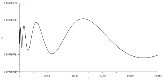
Figure 2: The wave of the first zero

The wave of the first zero occupies most of the oscillatory part, if the Riemann hypothesis is true, every zeros are simple and $c_{\gamma}$ is of rapid decay as ${\operatorname{Im}}(\gamma)\to\infty$ (very plausible since $\Gamma(\gamma)$ is rapidly decreasing). Here is a numerical data

$$c_{\gamma_{1}} = 3.011993987\cdots 10^{-11}+4.792386731\cdots 10^{-10}\sqrt{-1},$$

$$c_{\gamma_{2}} = -5.721173997\cdots 10^{-15}+1.369306521\cdots 10^{-14}\sqrt{-1},$$

$$c_{\gamma_{3}} = -2.705070957\cdots 10^{-17}+2.213981113\cdots 10^{-17}\sqrt{-1}$$

for ${\operatorname{Im}}(\gamma_{2})=21.02203963\cdots$ and ${\operatorname{Im}}(\gamma_{3})=25.01085758\cdots$. Comparing Figure 2 and the table of ${\mathcal{N}}(n)$, we see that the amplitude of the wave is still much smaller than the error term for $x\leq 100000$. However, it gets larger as $x$ increases. From Figure 2, the reader can guess how it grows.

References

- [1] L. Báez-Duarte: Hardy-Ramanujan’s asymptotic formula for partitions and the central limit theorem, Adv. Math. 125 (1997) 114–120.
- [2] W. Bosma, J. Cannon and C. Playoust: The Magma algebra system. I. The user language, Journal of Symbolic Computation 24, 235–265 (1997)
- [3] J. Cannon, et al.: Magma a Computer Algebra System, School of Mathematics and Statistics, University of Sydney, 2017. http://magma.maths.usyd.edu.au/magma/
- [4] H. Cramér: Random variables and probability distributions. Third edition. Cambridge Tracts in Mathematics and Mathematical Physics, No. 36 Cambridge University Press, London-New York 1970.
- [5] G. Harder and M. S. Narasimhan: On the cohomology groups of moduli spaces of vector bundles on curves. Math. Ann. 212 (1975) Issue 3, 215–248.
- [6] G. H. Hardy and S. Ramanujan: Asymptotic Formulaæ in Combinatory Analysis. Proc. London Math. Soc. S2-17 (1918), no. 1, 75–115.
- [7] Yu. I. Manin: The theory of commutative formal groups over fields of finite characteristic. Uspehi Mat. Nauk 18 (1963) no. 6 (114), 3–90; Russ. Math. Surveys 18 (1963), 1-80.
- [8] G. Meinardus: Asymptotische Aussagen über Partitionen. Math. Z. 59 (1954) 388–398.
- [9] B. Riemann: Ueber die Anzahl der Primzahlen unter einer gegebenen Grösse. Monatsberichte der Berliner Akademie, November 1859.
- [10] E. C. Titchmarsh: The theory of the Riemann zeta-function. Second edition. Edited and with a preface by D. R. Heath-Brown. The Clarendon Press, Oxford University Press, New York, 1986.
-
[11]
Maple User Manual: Toronto: Maplesoft, a division of Waterloo Maple Inc., 2016., available on the web page
http://www.maplesoft.com/products/maple/ -
[12]
Computation programs and log files for the paper “Asymptotic formula of the number of Newton polygons”, available on the web page
http://www.h-lab.ynu.ac.jp/AFofNP.html