More than one Author with different Affiliations

Smooth backfitting of proportional hazards with multiplicative components

Abstract

Smooth backfitting has proven to have a number of theoretical and practical advantages in structured regression. By projecting the data down onto the structured space of interest smooth backfitting provides a direct link between data and estimator. This paper introduces the ideas of smooth backfitting to survival analysis in a proportional hazard model, where we assume an underlying conditional hazard with multiplicative components. We develop asymptotic theory for the estimator. In a comprehensive simulation study we show that our smooth backfitting estimator successfully circumvents the curse of dimensionality and outperforms existing estimators. This is especially the case in difficult situations like high number of covariates and/or high correlation between the covariates, where other estimators tend to break down. We use the smooth backfitter in a practical application where we extend recent advances of in-sample forecasting methodology by allowing more information to be incorporated, while still obeying the structured requirements of in-sample forecasting.

1 Introduction

Nonparametric models suffer from the curse of dimensionality in high dimensional data spaces. Random forests (Breiman:01) circumvent the dimensionality problem by assuming that not all variables are relevant and that the function of interest can be approximated well by piecewise constant functions; see Wright:Ziegler:17 for a recent survival implementation. An alternative is to introduce some structure that stabilizes the system. Introducing structure has the additional advantage that it allows to visualize, interpret, extrapolate and forecast the properties of the underlying data. In this paper, we concentrate on structured models. The smooth backfitting algorithm of Mammen:etal:99 consideres the simplest nonparametric structure in the regression context - the additive structure. It has many theoretical and practical advantages to earlier approaches of regression backfitting. The popular regression backfitting approach of Hastie:Tibshirani:90 are numerical iterating-procedures estimating one component given the estimates of the rest. In contrast, smooth backfitting is a direct projection of the data down onto the structured space of interest. This direct relationship between data and estimates gives a more solid grip on what is being estimated and the theoretical properties underlying it, see also Nielsen:Sperlich:05 and Huang:Yu:19. The purpose of this paper is to introduce smooth backfitting to the field of survival analysis and nonparametric smooth hazard estimation. While the additive structure is the most natural and most widely used in regression, the multiplicative structure seems more natural in hazard estimation. The omnipresent Cox regression model is a proportional hazard model (also known as Cox proportional hazard model) and many extensions and alternatives to the Cox regression model have been formulated in a multiplicative framework. We will therefore consider the multiplicative structure in this paper. It can be used in applications to test Cox regression or other proportional hazard models either visually or quantitatively. But this is beyond the scope of this paper. Multiplicative smooth backfitting is theoretically more challenging than additive smooth backfitting. The smooth backfitting multiplicative regression structure was analysed by Yu:etal:08 as a special case of generalized additive models. Yu:etal:08 showed that the multiplicative structure - in contrast to the simpler additive case - provides asymptotic theory with a number of non-trivial interactions between exposure available in different directions. Naturally, the asymptotics provided here for smooth backfitting of multiplicative hazards contains similar interactive components in the asymptotic theory. The survival projection introduced in this paper is different and less intuitive than the nonparametric regression considered in Mammen:etal:99; Mammen:etal:01. As in density estimation, see Jones:93, hazard estimation requires a projection of a dirac-delta-sequence related to the jumps of the counting process, see also Nielsen:98 and Nielsen:Tanggaard:01. We provide a simple algorithm first projecting the data down onto an unstructured estimator, and then further projecting the unstructured estimator down onto the multiplicative space of interest. Our numerical algorithms are greatly simplified by a new principle of weighting the projection according to the final estimates.

We consider a multiplicatively structured proportional hazard model:

$$\alpha(t,z)=\alpha_{0}(t)\alpha_{1}(z_{1})\cdots\alpha_{d}(z_{d}),$$ (1.1)

where $\alpha_{k},$ $k=0,\dots,d$, are some smooth and positive one-dimensional functions and $z=(z_{1},\dots,z_{d})\in\mathbb{R}^{d}$ are possibly time $t$-dependent covariates. We do not impose any further structural assumption on $\alpha_{k}$. This is in contrast to the semiparametric Cox proportional hazard model where all components, with exception of the baseline hazard $\alpha_{0}$, are assumed to take a log-linear shape. We do expect that smooth backfitting of proportional hazard models can be generalized to much the same way as the Cox proportional hazard model is generalized. As one recent example that could be interesting to treat as a smooth backfitting problem, see Hsu:etal:18.

Estimators for model (1.1) can be categorized in four groups: (i) Therneau:etal:90 and Grambsch:etal:95 start with the Cox model and investigate smoothed residual plots; (ii) Hastie:Tibshirani:90; Hastie:Tibshirani:90b, OSullivan:88; OSullivan:93, Sleeper:Harrington:90 and Huang:99 consider splines via penalized partial likelihood; (iii) Linton:etal:03, Honda:05 build on marginal integration (Linton:Nielsen:95) and (iv) Lin:etal:16 use kernel smoothers starting from a global partial likelihood criterion.

Lin:etal:16 prove asymptotic efficiency of their estimator and they show by a detailed simulation study that their estimator outperforms the proposals in Huang:99, Linton:etal:03, Honda:05. For this reason in this paper we take their estimator as benchmark. It has been argued that in additive regression models smooth backfitting is less affected by sparseness of high-dimensional data and by strong correlated covariables, see Nielsen:Sperlich:05. In this paper we will show that this also holds for our smooth backfitter in a multiplicatively structured proportional hazard model. For this purpose we study the smooth backfitter in settings which include challenging high dimensional data and highly correlated covariates. The smooth backfitting approach turns out to show a very good performance compared to all other estimators and to be very robust to both, high dimensional and correlated data. In particular in high-dimensional settings it strongly outperforms the approach of Lin:etal:16 that already for low dimensions runs into instabilities and numerical problems. In this paper, we do not treat the problem of variable selection. It would in particular be interesting to investigate Lasso approaches or nonparametric tests on the significance of one component. For the development of tests our theory may be used as a first step.

The paper is structured as follows. Section 2 contains the mathematics of the underlying survival model. In Section 3 the smooth backfitting estimator is defined as a projection of unstructured hazard estimators. This is done for unstructured hazard estimators that can be written as a ratio of smooth occurrence and smooth exposure. An example is given by the local constant Nadaraya-Watson estimator. In Section 4 asymptotic properties are outlined for the smooth backfitting estimator. Details are explained in the Supplementary Material of this paper. Section 5 contains our finite sample study illustrating the strong performance of smooth backfitting. In Section 6 we consider a sophisticated version of in-sample forecasting generalising earlier approaches via our proportional hazard model, see Mammen:etal:15, Hiabu:etal:16 Lee:etal:15; Lee:etal:17; Lee:etal:18a. A smooth extension of the popular actuarial chain ladder model that is used in virtually all non-life insurance companies in the world while estimating outstanding liabilities. In-sample forecasting is possible because of the imposed multiplicative structure.

2 Aalen’s multiplicative intensity model

We consider a counting process formulation satisfying Aalen’s multiplicative intensity model. It allows for very general observations schemes. It covers filtered observations arising from left truncation and right censoring and also more complicated patterns of occurrence and exposure. In the next section we describe how to embed left truncation and right censoring into this framework. In contrast to Linton:etal:03 we will hereby allow the filtering to be correlated to the survival time and be represented in the covariate process. We briefly summarize the general model we are assuming.
We observe $n$ $iid$ copies of the stochastic processes $(N(t),Y(t),Z(t)),\ t\in[0,R_{0}],\,R_{0}>0.$ Here, $N$ denotes a right-continuous counting process which is zero at time zero and has jumps of size one. The process $Y$ is left-continuous and takes values in $\{0,1\}$ where the value $1$ indicates that the individual is under risk. Finally, $Z$ is a $d$-dimensional left-continuous covariate process with values in a hyperrectangle $\prod_{j=1}^{d}[0,R_{j}]\subset\mathbb{R}^{d}$.The multivariate process $((N_{1},Y_{1},Z_{1}),\dots,(N_{n},Y_{n},Z_{n}))$, $\ i=1,\dots,n$, is adapted to the filtration $\mathcal{F}_{t}$ which satisfies les conditions habituelles (the usual conditions), see Andersen:etal:93 (pp. 60). Now we assume that $N_{i}$ satisfies Aalen’s multiplicative intensity model, that is

$$\lambda_{i}(t)=\lim_{h\downarrow 0}h^{-1}E[N_{i}((t+h)-)-N_{i}(t-)|\ \mathcal{F}_{t-}]=\alpha(t,Z_{i}(t))Y_{i}(t).$$ (2.1)

The deterministic function $\alpha(t,z)$ is called hazard function and it is the failure rate of an individual at time $t$ given the covariate $Z(t)=z$.

2.1 Left truncation and right censoring time as covariates

The most prominent example for Aalen’s multiplicative intensity model is filtered observation due to left truncation and right censoring. We now show how to embed model (1.1) with covariate, $Z$, possibly carrying truncation and censoring information into Aalen’s multiplicative intensity model. Every covariate coordinate can carry individual truncation information as long as it corresponds to left truncation. That is, we observe $(T,Z)$ if and only if $(T,Z(T))\in\mathcal{I}$, where the set $\mathcal{I}$ is compact and it holds that if $(t_{1},Z(t_{1}))\in\mathcal{I}$ and $t_{2}\geq t_{1},\text{then}$ $(t_{2},Z(t_{2}))\in\mathcal{I},\ a.s..$ The set $\mathcal{I}$ is allowed to be random but is independent of $T$ given the covariate process $Z$. Furthermore, $T$ can be subject to right censoring with censoring time $C$. We assume that also $T$ and $C$ are conditional independent given the covariate process $Z$. This includes the case where the censoring time equals one covariate coordinate. In conclusion, we observe $n$ $iid$ copies of $(\widetilde{T},Z^{*},\mathcal{I},\delta)$, where $\delta=\mathds{1}(T^{*}<C),\ \widetilde{T}=\min(T^{*},C)$, and $(T^{*},Z^{*})$ is the truncated version of $(T,Z)$, i.e, $(T^{*},Z^{*})$ arises from $(T,Z)$ by conditioning on the event $(T,Z(T))\in\mathcal{I}$.

Then, for each subject, $i=1,\ldots,n$, we can define a counting process $N_{i}$ as $N_{i}(t)=\mathds{1}\left\{\widetilde{T}_{i}\leq t,\ \delta_{i}=1\right\},$ with respect to the filtration $\mathcal{F}_{i,t}=\sigma\left(\bigg{\{}\widetilde{T}_{i}\leq s,\ Z^{*}_{i}(s),\ \mathcal{I}_{i},\ \delta_{i}:\ s\leq t\bigg{\}}\cup\mathcal{N}\right),$ where $\mathcal{N}$ is a class of null-sets that completes the filtration. After straightforward computations one can conclude that under the setting above, Aalen’s multiplicative intensity model (2.1) is satisfied with

$$\alpha_{z}(t) =\alpha(t,z)=\lim_{h\downarrow 0}h^{-1}\mathrm{Pr}\{T_{i}\in[t,t+h)|\ T_{i}\geq t,\ Z_{i}(t)=z\},$$

$$Y_{i}(t) =\mathds{1}\big{\{}(t,Z^{*}_{i}(t))\in\mathcal{I}_{i},\ t\leq\widetilde{T}_{i}\big{\}}.$$

3 Estimation

We tackle the problem in two steps. First the data are projected down onto an unstructured space resulting in an unstructured estimator of the $d+1-$dimensional hazard function $\alpha(t,z)$; see (1.1). In the second step, the unstructured estimator is projected further down onto the multiplicative space of interest resulting in $d+1$ one-dimensional smooth backfitting estimators of the multiplicative components, $(\alpha_{0}(t),\alpha_{1}(z_{1}),\dots,\alpha_{d}(z_{d}))$. For the first step we assume to have an unstructured estimator with simple ratio of smoothed occurrence and smoothed exposure. Our theory will encompass all estimators with this simple ratio structure. We discuss in Section 4 and in the accompanied Supplementary Material that our estimation procedure works under quite general assumptions. In particular we do not need the unstructured estimator of the first step to be consistent. The final structured estimator circumvents the curse of dimensionality even if consistency is not assured in the first step. This is reassuring noting that the unstructured estimator will most probably have exponentially deteriorating performance with growing dimension $d$.

We introduce the notation $X_{i}(t)=\left(t,Z_{i}(t)\right)$. We also set $x=(t,z)$, with coordinates $x_{0}=t,\ x_{1}=z_{1},\dots,x_{d}=z_{d}$, and write the hazard as $\alpha(t,z)=\alpha(x)$.

3.1 First step: The unstructured estimator

To estimate the components of the structured hazard in (3.2) below, we will need an unstructured pilot estimator of the hazard $\alpha$ first. We propose the local constant kernel estimator, $\widetilde{\alpha}^{LC}$. Its value in $x$ is defined as

$$\widetilde{\alpha}^{LC}(x)=\lim_{\varepsilon\to 0}\arg\min_{\theta_{0}\in\mathbb{R}}\sum_{i=1}^{n}\int \left\{\frac{1}{\varepsilon}\int_{s}^{s+\varepsilon}\mathrm{d}N_{i}(u)-\theta_{0}\right\}^{2}$$ (3.1)

$$\quad\times\kappa_{n}(X_{i}(s))K_{b}(x-X_{i}(s))Y_{i}(s)\ \mathrm{d}s.$$

In the following, we restrict ourselves to a multiplicative kernel, i.e., for , $(u_{0},\dots,u_{d})\in\mathbb{R}^{d+1}$, $K(u_{0},\dots,u_{d})=\prod_{j=0}^{d}k(u_{j})$, and a one-dimensional bandwidth $b$ with boundary correction $\kappa_{n}(x)=\prod_{j=0}^{d}\left(\int K_{b}(x_{j}-u_{j})\ du_{j}\right)^{-1}$ and $K_{b}(u)=\prod_{j=0}^{d}b^{-1}k(b^{-1}u_{j})$, where for simplicity of notation the bandwidth $b>0$ does not depend on $j$. More general choices would have been possible with the cost of extra notation.

We get $\widetilde{\alpha}^{LC}(x)=\widehat{O}^{LC}(x)/\widehat{E}^{LC}(x)$, with smoothed occurrence and smoothed exposure given by

$$\widehat{O}^{LC}(x) =\sum_{i=1}^{n}\int\kappa_{n}(X_{i}(s))K_{b}(x-X_{i}(s))\mathrm{d}N_{i}(s),$$

$$\widehat{E}^{LC}(x) =\sum_{i=1}^{n}\int\kappa_{n}(X_{i}(s))K_{b}(x-X_{i}(s))Y_{i}(s)\mathrm{d}s.$$

Under standard smoothing conditions, if $b$ is chosen of order $n^{-1/(4+d+1)}$, then the bias of $\widetilde{\alpha}^{LC}(x)$ is of order $n^{-2/(4+d+1)}$ and the variance is of order $n^{-4/(4+d+1)}$, which is the optimal rate of convergence in the corresponding regression problem, see Stone:82. For an asymptotic theory of these estimators see Linton:etal:03.

3.2 Second step: The structured smooth backfitting estimator

In this section we will project the unstructured estimator of the previous section down onto the multiplicative space of interest. Other choices that have a simple ratio structure of occurrence and exposure are possible. Due to filtering, observations are assumed to be only available on a subset of the full support, $\mathcal{X}\subseteq\mathcal{R}=\prod_{j=0}^{d}[0,R_{j}]$. Our estimators are restricted to this set and detailed assumptions on $\mathcal{X}$ and the data generating functions are given in the Supplementary Material. Our calculations simplify via a new principle we call solution-weighted minimization. We assume that we have the solution and use it strategically in the least squares weighting. While the definition is not explicit, it is made feasible by defining it as an iterative procedure. In the sequel we will assume a multiplicative structure of the hazard $\alpha$, i.e.,

$$\alpha(x)=\alpha^{*}\prod_{j=0}^{d}\alpha_{j}(x_{j}),$$ (3.2)

where $\alpha_{j}$, $j=0,\dots,d,$ are some functions and $\alpha^{*}$ is a constant. For identifiability of the components, we make the following further assumption:

$$\int\alpha_{j}(x_{j})w_{j}(x_{j})\ \mathrm{d}x_{j}=1,\quad j=0,\dots,d,$$

where the $w_{j}$’s are some weight functions.

We also need the following notation:

$$F_{t}(z)=Pr\left(Z_{1}(t)\leq z|\ Y_{1}(t)=1\right),\quad y(t)=E[Y_{1}(t)].$$

By denoting $f_{t}(z)$ the density corresponding to $F_{t}(z)$ with respect to the Lebesgue measure, we also define $E(x)=f_{t}(z)y(t)$ and $O(x)=E(x)\alpha(x)$.

We define the estimators $\widehat{\alpha}^{*}$ and $\widehat{\alpha}=(\widehat{\alpha}_{0},\dots,\widehat{\alpha}_{d})$ of the hazard components in (3.2) as solution of the following system of equations:

$$\widehat{\alpha}_{k}(x_{k})=\frac{\int_{\mathcal{X}_{x_{k}}}\widehat{O}(x)\mathrm{d}x_{-k}}{\int_{\mathcal{X}_{x_{k}}}\widehat{\alpha}^{*}\prod_{j\neq k}\widehat{\alpha}_{j}(x_{j})\widehat{E}(x)\mathrm{d}x_{-k}},\quad k=0,\dots,d,$$ (3.3)

$$\int\widehat{\alpha}_{k}(x_{k})w_{k}(x_{k})\ \mathrm{d}x_{k}=1,\quad k=0,\dots,d.$$ (3.4)

Here $\mathcal{X}_{x_{k}}$ denotes the set $\{(x_{0},\dots,x_{k-1},x_{k+1},\dots,x_{d})|\ (x_{0},\dots,x_{d})\in\mathcal{X}\}$, and
$x_{-k}=(x_{0},\dots,x_{k-1},x_{k+1},\dots,x_{d})$. Furthermore, $\widehat{E}$ and $\widehat{O}$ are some full-dimensional estimators of $E$ and $O$ – not necessarily the one provided in the previous section. We will discuss in the Supplementary Material that the system above has a solution with probability tending to one. In the next section and in the Supplementary Material we will show asymptotic properties of the estimator. We will see that we do not require that the full-dimensional estimators $\widehat{E}$ and $\widehat{O}$ are consistent. We will only need asymptotic consistency of marginal averages of the estimators. This already highlights that our estimator efficiently circumvents the curse of dimensionality.

In practice, system (3.3) can be solved by the following iterative procedure:

$$\widehat{\alpha}_{k}^{(r+1)}(x_{k})=\frac{\int_{\mathcal{X}_{x_{k}}}\widehat{O}(x)\mathrm{d}x_{-k}}{\int_{\mathcal{X}_{x_{k}}}\prod_{j=0}^{k-1}\widehat{\alpha}_{j}^{(r+1)}(x_{j})\prod_{j=k+1}^{d+1}\widehat{\alpha}_{j}^{(r)}(x_{j})\widehat{E}(x)\mathrm{d}x_{-k}},\quad k=0,\dots,d$$ (3.5)

After a finite number of cycles or after a termination criterion applies, the last values of $\widehat{\alpha}_{k}^{(r+1)}(x_{k})$, $k=0,...,d$, are multiplied by a factor such that the constraint (3.4) is fulfilled. This can always be achieved by multiplication with constants. This gives the backfitting approximations of $\widehat{\alpha}_{k}(x_{k})$ for $k=0,...,d$.

3.3 Interpretation as direct projection

The strength of our smooth backfitting estimator is that it can be motivated directly from a least squares criterium on the data without ad-hoc adjustment. The estimator $\widehat{\alpha}$ can be motivated as solution of

$$\lim_{\varepsilon\to 0}\arg\min_{\theta}\sum_{i=1}^{n}\int\int \Bigg{\{}\frac{1}{\varepsilon}\int_{s}^{s+\varepsilon}\mathrm{d}N_{i}(u)-\theta(x)\Bigg{\}}^{2} \times K_{b}(x-X_{i}(s))Y_{i}(s)\ \mathrm{d}s\ \mathrm{d}\nu(x),$$ (3.6)

where $\theta$ runs over some space of smooth multiplicative functions of the form $\theta=\prod_{j=0}^{d}\theta_{j}(x_{j})$. To see this, consider the estimator $\overline{\alpha}=(\overline{\alpha}^{*},\overline{\alpha}_{0},\dots,\overline{\alpha}_{d})$ that minimizes

$$\arg\min_{\overline{\alpha}}\int_{\mathcal{X}}\left\{\widetilde{\alpha}^{LC}(x)-\overline{\alpha}^{*}\prod_{j=0}^{d}\overline{\alpha}_{j}(x_{j})\right\}^{2}w(x)\mathrm{d}x.$$ (3.7)

For $\nu(x)=w(x)/\widehat{E}^{LC}(x)dx$ the solution of (3.7) is exactly (3.6). With that choice, we get

$$\overline{\alpha}^{*}=\frac{\int_{\mathcal{X}}\widetilde{\alpha}(x)\prod_{j=0}^{d}\overline{\alpha}_{j}(x_{j})w(x)\mathrm{d}x}{\int_{\mathcal{X}}\left\{\prod_{j=0}^{d}\overline{\alpha}_{j}(x_{j})\right\}^{2}w(x)\mathrm{d}x},$$

and $(\overline{\alpha}_{0},\dots,\overline{\alpha}_{d})$ can be described via the backfitting equation

$$\overline{\alpha}_{k}(x_{k})=\frac{\int_{\mathcal{X}_{x_{k}}}\widetilde{\alpha}(x)\prod_{j\neq k}\overline{\alpha}_{j}(x_{j})w(x)\mathrm{d}x_{-k}}{\int_{\mathcal{X}_{x_{k}}}\overline{\alpha}^{*}\left\{\prod_{j\neq k}\overline{\alpha}_{j}(x_{j})\right\}^{2}w(x)\mathrm{d}x_{-k}},\quad k=0,\dots,d.$$ (3.8)

The asymptotic variance of kernel estimators of $\alpha$ is proportional to $\alpha(x)/E(x)$, see e.g. Linton:Nielsen:95. This motivates the choice $w(x)=E(x)/\alpha(x)$. However, this choice is not possible because $E(x)$ and $\alpha(x)$ are unknown. One could use $w(x)=\check{E}(x)/\check{\alpha}(x)$ where $\check{E}(x)$ and $\check{\alpha}(x)$ are some pilot estimators of $E$ and $\alpha$. We follow another idea and we propose to weight the minimization (3.7) with its solution. We choose

$$w(x) =\frac{\widehat{E}(x)}{\prod_{i}\widehat{\alpha}_{i}(x)},$$ (3.9)

and heuristically, by putting $\overline{\alpha}_{j}=\widehat{\alpha}_{j}$ and by plugging (3.9) into (3.8), we get (3.3).

4 Asymptotic properties of the smooth backfitter of multiplicative hazards

In the Supplementary Material we show that $\widehat{\alpha}_{j}$ converges to the true $\alpha_{j}$ with optimal one dimensional nonparametric rate $n^{-2/5}$, given that the bandwidth $b$ is chosen of order $n^{-1/5}$. This means in particular that the asymptotic rate does not depend on the dimension $d$. Under regularity assumptions, in Theorem 3 in the Supplementary Material we show that

$$n^{2/5}\{(\widehat{\alpha}_{j}-\alpha_{j})(x_{j})-\alpha_{j}(x_{j})B_{j}(x_{j}))\}\rightarrow\mbox{N}(0,\alpha^{2}_{j}(x_{j})\sigma_{j}^{2}(x_{j})),$$

where $B_{j}(x_{j})$ can be formally defined as the $j$-th component of a projection of the bias of the unconstrained estimator onto the multiplicative space and $\sigma_{j}^{2}(x_{j})$ is the variance of a weighted average of the unconstrained estimator where the other components are integrated out.

In the simulation study of the next section we show that estimation seems to work well even when $d$ is of similar order as $n$. This is, we believe, a major strength of our smooth backfitting estimator.

A few notes on the proof. The estimator $\widehat{\alpha}_{j}$ is defined as solution of a nonlinear operator equation. Asymptotic properties are derived by approximating the estimators of this equation by a linear equation that can be interpreted as one equation that arises in nonparametric additive regression models (Mammen:etal:99), and then one shows that the solution of the linear equation approximates the estimation error in the multiplicative model. The linear equation and its solution is well understood from the theory of additive models. This is our essential step to arrive at an asymptotic understanding of our estimator $\widehat{\alpha}_{j}$. Assumptions are of standard nature in marker dependent hazard papers and they can be verified for the local constant estimators we are interested in, see in particular Nielsen:Linton:95, Nielsen:98 and Linton:etal:03 for related arguments. However, the conditions are formulated more general and they are not restricted to the local constant smoothers. They are not even tight to kernel smoothers. Any smoother could be used as long as it obeys the structure of being a ratio of a smoothed occurrence and a smoothed exposure.

5 Simulation study

In this section we present detailed simulations of the smooth backfitter. The Supplementary Material contains additional simulation results for the setting discussed in Honda:05 and Lin:etal:16. In these latter settings, the performance of the smooth backfitter is similar to the estimator of Lin:etal:16. And both estimators outperform the estimators considered in Honda:05.

In the simulation study below, and with additional results in The Supplementary Material, we compare our estimator with the estimator of Lin:etal:16. The models of these simulations contain high-dimensional and correlated covariates and in particular, we will show that our estimator – in contrast to Lin:etal:16 – works in high dimensions where the dimension of the covariates is of similar order as the sample size and also in cases with higher correlation between the covariates. To highlight the impact of increasing dimension we will consider the dimensions $d=2$ and $d=9$. Further results for dimensions $d=30$ and $d=99$ can be found in the Supplementary Material. The low dimensional setting, $d=2$, with uncorrelated covariates is similar to the setting of Honda:05 and Lin:etal:16, and the difference between our estimator and the estimator of Lin:etal:16 are indeed marginal in this case. However, below and in the Supplementary Material we show that this changes drastically with increasing dimension and/or correlation.

5.1 The setting

Since the estimator of Lin:etal:16 is based on a partial likelihood approach, it does not estimate the baseline hazard, $\alpha_{0}$. We will consider the sub-model

$$\alpha(x)=\prod_{k=0}^{d}\alpha_{k}(x_{k})=\exp\left\{\sum_{k=1}^{d}\eta_{k}(x_{k})\right\},$$

i.e., we assume a constant baseline hazard, $\alpha_{0}\equiv 1$. More specifically, we assume that the survival times $T_{i}$ follow an exponential distribution with parameter value $\alpha(X_{i}),\quad(i=1,\dots,n)$. We add right censoring with censoring variables $C_{i}$ that follow an exponential distribution with parameter $\frac{4}{7}\alpha(X_{i}),\quad(i=1,\dots,n)$. We will compare the estimators for $\eta_{k},k=1,\dots,d$. Our proposed estimator is derived as $\widehat{\eta}_{k}^{SBF}=\log(\widehat{\alpha}_{k})$ and we compare it to, $\widehat{\eta}_{k}^{\text{Lin et al.}}$, proposed in Lin:etal:16.

We used the following two models:

$$\text{Model 1: }\eta_{k}(z_{k})=\begin{cases}-z_{k}\quad&\text{if k is odd,}\\ 2z_{k}\quad&\text{if k is even.}\end{cases}$$

$$\text{Model 2: }\eta_{k}(z_{k})=\begin{cases}2\sin(\pi z_{k})\quad&\text{if k is odd,}\\ 2z_{k}\quad&\text{if k is even.}\end{cases}$$

The covariates $(Z_{i1},\dots,Z_{id})$ are generated as follows. We first simulate $(\widetilde{Z}_{i1},\dots,\widetilde{Z}_{id})$ from a $d$-dimensional multi-normal distribution with mean equal 0 and $\textrm{Corr}(Z_{ij},Z_{il})=\rho$ if $j\neq l,$ else 1. Afterwards we set

$$Z_{ik}=2.5\pi^{-1}\text{arctan}(\widetilde{Z}_{ik}).$$

This has been independently repeated for every individual $i=1,\dots,n$. After trying several bandwidths, if not said otherwise, we present the results for a bandwidth $b=0.3$ for both estimators in every model. As kernel function k, we used the Epanechnikov kernel. Performance is measured via the integrated squared error evaluated at the observed points:

$$ISE_{k}=n_{obs}^{-1}\sum_{i_{obs}}\left(\eta_{k}(Z_{i_{obs}k})-\widehat{\eta}_{k}(Z_{i_{obs}k})\right)^{2},$$

$$ISE_{odd}=\{ISE_{k}|k=odd\},\quad ISE_{even}=\{ISE_{k}|k=even\},\quad$$

where $i_{obs}$ runs over all observed individuals and $n_{obs}<n$ is the number of observed individuals. The next two subsections discuss the outcomes of the simulations for $d=2$ and $d=9$.

5.2 Dimension $d=2$

In low dimensions both estimators perform satisfactorily. Already in dimension $d=2$, for Model 1, it occurred that the algorithm of Lin:etal:16 stopped before the final calculation of the estimator. This happened for three simulation samples out of 1200 ($6$ settings $\times 200$ samples each) runs. The algorithm stopped at a step where a matrix has to be inverted that is nearly singular. In contrast, our estimator does not need to invert matrices and we did not have any singularity or convergence issues for our estimator. Performance-wise, we refer to Figure 2 displaying boxplots of the integrated squared errors of both estimators. The two estimators perform similar with a small advantage towards our smooth backfitting estimator. The smooth backfitting estimator performs especially better for the smaller sample size $n=200$. While Lin:etal:16 performed better in Model 2 with no correlation, the performance of the smooth backfitting estimator seems more stable when correlation is added. Figure 1 shows the 200 sample estimates of the first component $\alpha_{1}$ of Model 2 with $\rho=0.8$. The estimator of Lin:etal:16 struggles especially at the boundaries and this is more pronounced with a small bandwidth (left panel). If bandwidth is increased (right panel), the estimate of Lin:etal:16 seems over-smoothed and it is not able to replicate the full magnitude of the local extrema at $-0.5$ and $-0.5$.

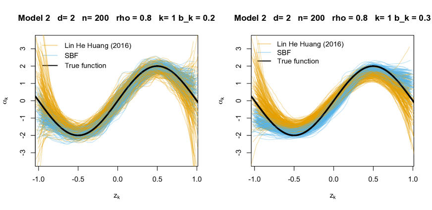
Figure 1: Estimates of $\alpha_{1}$ from 200 simulations. Left panel uses a bandwidth of 0.2 and right panel a bandwidth of 0.3.

Figure 2: Boxplots of the integrated squared errors. Simulations are taken out where the algorithm for the calculation of the estimator in Lin:etal:16 stopped without calculation of all values of the estimator. The value $n.sim$ is the number of the remaining simulations, i.e., 200 minus number of break downs.

5.3 Dimension $d=9$

When the dimension $d$ is increased to 9, the estimator of Lin:etal:16 breaks down considerably more often than in the case $d=2$, i.e., in 59 (4+5+48+1+1 out of 1200) cases in Model 1 and 9 times in Model 2; see Table 1. Note that in the more extreme cases of $d=99$, provided in the Supplementary Material, nearly all simulations of Lin:etal:16 (780 and 607 out of 800 for Model 1 and Model 2, respectively) broke down. In contrast, our estimator converged in all cases considered. Performance-wise we refer to Figure 4 displaying boxplots of the integrated squared errors of both estimators. We see that for $d=9$ the smooth backfitter performs better in every setting. The better performance is more pronounced when more correlation is present. Figure 3 shows 200 sample estimates of the first component $\alpha_{1}$ of Model 2 with $\rho=0.8$. The results are similar as in the case $d=2$, but now more pronounced: The estimator of Lin:etal:16 struggles at the boundaries and if bandwidth is increased (right panel), the estimate of Lin:etal:16 seems too smooth and is not able to replicate to full magnitude of the local extrema at $-0.5$ and $-0.5$.

Number of breakdowns in Lin:etal:16 for $d=9$
(out of 200 simulations)
	Model 1			Model 2
	$\rho=0$	$\rho=0.5$	$\rho=0.8$	$\rho=0$	$\rho=0.5$	$\rho=0.8$
n=200	4	5	48	0	0	9
n=500	0	1	1	0	0	0

Table 1: Number of breakdowns in the algorithm of Lin:etal:16 out of 200 simulations for dimension $d=9$.

Figure 3: Estimates of $\alpha_{1}$ from 200 simulations. Left panel uses a bandwidth of 0.2 and right panel a bandwidth of 0.3.

Figure 4: Boxplots of the integrated squared errors. Simulations are taken out where the algorithm for the calculation of the estimator in Lin:etal:16 stopped without calculation of all values of the estimator. The value $n.sim$ is the number of the remaining simulations, i.e., 200 minus number of break downs.

6 In-sample forecasting of outstanding loss liabilities

The so-called chain ladder method is a popular approach to estimate outstanding liabilities. It started off as a deterministic algorithm, and it is used today for almost every single insurance policy over the world in the business of non-life insurance. In many developed countries, the non-life insurance industry has revenues amounting to around 5%. It is therefore comparable to - but smaller than - the banking industry. In every single product sold, the chain ladder method (because actuaries hardly use other methods) comes in, estimating the outstanding liabilities that eventually aggregate to the reserve - the single biggest number of most non-life insurers balance sheets. The insurers liabilities often amount to many times the underlying value of the company. In Europe alone those outstanding liabilities are estimated to accumulate to around € 1$trn.Itisthereforeofobviousimportancethatthisestimateisnottoofarfromthebestpossibleestimate.Wedescribeinthissectionhowthemethodologyintroducedinthispapercanbeappliedtoprovideasolutiontothischallengingproblem.\par WeanalyzereportedclaimsfromamotorbusinesslineinCyprus.Thesamedatasethasbeenusedby\cite[citet]{\@@bibref{Authors Phrase1YearPhrase2}{Hiabu:etal:16}{\@@citephrase{(}}{\@@citephrase{)}}}anditconsistsofthenumberofclaimsreportedbetween2004and2013.Duringthese$10$years(3654days),$n=58180$claimswerereported.Thedataaregivenas${(T_1,Z_1),…, (T_n,Z_n)}$,where$Z_i$denotestheunderwritingdateofclaim$i$,and$T_i$thetimebetweenunderwritingdateandthedateofreportofaclaimindays,alsocalledreportingdelay.Hence,inthenotationoftheprevioussections,thecovariateunderwritingdate,$Z(t)=Z$,doesnotdependontimeandhasdimension$d=1$.Thedataexistonatriangle,with$T_i + Z_i ≤31 December 2013=R_0$,whichisasubsetofthefullsupport$R=[0,R_0]^2$($0=1  January   2004$).Theaimistoforecastthenumberoffutureclaimsfromcontractswritteninthepastwhichhavenotbeenreportedyet.Figure\ref{histo}showstheobserveddatathatlieonatriangle,whiletheforecastsarerequiredonthetrianglethataddedtothefirstcompletesasquare.Hereitisimplicitlyassumedthatthemaximumreportingdelayofaclaimis$10$years.Actuariescallthisassumptionthatthetriangleisfullyrunoff.Inourdataset,thisisareasonableassumptionlookingatFigure\text{<a href="\#S6.F5" title="Figure 5 ‣ 6 In-sample forecasting of outstanding loss liabilities ‣ More than one Author with different Affiliations" class="ltx\_ref ltx\_font\_italic"><span class="ltx\_text ltx\_ref\_tag">5</span></a>}.\text{Figure 55Figure 55Histogramofclaimnumbersofamotorbusin}$