A Real-Time Solver For Time-Optimal Control Of
Omnidirectional Robots with Bounded Acceleration

Abstract

We are interested in the problem of time-optimal control of omnidirectional robots with bounded acceleration (TOC-ORBA). While there exist approximate solutions for such problems, and exact solutions with unbounded acceleration, exact solvers to the TOC-ORBA problem have remained elusive until now. In this paper, we present a real-time solver for true time-optimal control of omnidirectional robots with bounded acceleration. We first derive the general parameterized form of the solution to the TOC-ORBA problem by application of Pontryagin’s maximum principle. We then frame the boundary value problem of TOC-ORBA as an optimization problem over the parameterized control space. To overcome local minima and poor initial guesses to the optimization problem, we introduce a two-stage optimal control solver (TSOCS): The first stage computes an upper bound to the total time for the TOC-ORBA problem and holds the time constant while optimizing the parameters of the trajectory to approach the boundary value conditions. The second stage uses the parameters found by the first stage, and relaxes the constraint on the total time to solve for the parameters of the complete TOC-ORBA problem. Furthermore, we implement TSOCS as a closed loop controller to overcome actuation errors on real robots in real-time. We empirically demonstrate the effectiveness of TSOCS in simulation and on real robots, showing that 1) it runs in real time, generating solutions in less than 0.5ms on average; 2) it generates faster trajectories compared to an approximate solver; and 3) it is able to solve TOC-ORBA problems with non-zero final velocities that were previously unsolvable in real-time.

I Introduction

Omnidirectional robots find use in a variety of domains where high maneuverability is important, such as indoor service mobile robots [1], robot soccer [2], and warehouse automation [3]. Such robots rely on one of several wheel designs [4] to decouple the kinematic constraints along the three degrees of freedom, two for translation and one for rotation, necessary for motion on a plane. The dynamics of the omnidirectional drive is constrained by the specific layout of the wheel configuration, and the drive motor characteristics. Owing to the complexity of modelling the angle-dependent dynamic constraints imposed by every motor, omnidirectional drive systems may be simplified as having acceleration and velocity that are bounded uniformly in all directions [5]. However, despite such simplifications, the solution to the time-optimal control of omnidirectional robots with bounded acceleration remains elusive: while there have been time-optimal solutions for omnidirectional robots with unbounded acceleration [6], and approximate solutions to time-optimal control with bounded acceleration and bounded velocity [5], until now, there has been no solution to the true time-optimal control of omnidirectional robots with bounded acceleration.

In this paper, we present an algorithm for true time-optimal control of an omnidirectional robot with bounded acceleration (TOC-ORBA) but unbounded velocity. By applying Pontryagin’s maximum principle to the dynamics of the omnidirectional robot with bounded acceleration, we derive the necessary conditions for the solution to the TOC-ORBA problem, and the adjoint variables of the problem. By analyzing the adjoint-space formulation, we derive the parametric form of a solution to the TOC-ORBA problem. Given a specific problem with initial and final conditions, we frame the TOC-ORBA problem as a boundary-value problem, to solve for the parameters of the optimal trajectory that satisfy the initial and final conditions.

However, this boundary value problem cannot be solved analytically, and direct application of optimization solvers result in poor convergence rates and sub-optimal local minima [7]. We therefore decouple the full solution into two stages to overcome local minima. In the first stage, we first compute the upper bound for the total time of the TOC-ORBA problem by decomposing the problem into three linear motion segments that are always solvable analytically, but which will be sub-optimal. We hold the total trajectory time constant at this upper bound, and solve for the parameters of the trajectory to approach the boundary value conditions. Since the total time is held constant in the first stage, it may not be able to exactly satisfy the boundary conditions, but will typically find the correct shape of the optimal trajectory. In the second stage, we use the first stage solution as an initial guess, relax the constraint on the total time, and solve for the parameters that exactly satisfy the boundary conditions. Thus, our two-stage optimal control solver (TSOCS) is able to compute exact solutions to the TOC-ORBA problem.

We further show how TSOCS can be modified for practical use in an iterative closed-loop controller for real robots with inevitable actuation errors. We demonstrate the closed-loop TSOCS controller running in real time at 60Hz on real robots, taking 0.5ms on average to solve the TOC-ORBA problem. We present results from experiments over extensive samples from the TOC-ORBA problem space with simulated noisy actuation, as well as on real robots. The evaluation of TSOCS shows that it outperforms existing approximate solvers [5], and that it can solve for, and execute time-optimal trajectories with non-zero final velocities, which were previously not solvable. We further demonstrate how varying a hyperparameter in the TSOCS controller can be used to trade-off accuracy in final location vs. final velocity.

II Background and Related Work

Omnidirectional robots, also referred to as holonomic drive robots, are governed by the following system of ordinary differential equations:

$$\frac{dx_{1}}{dt}=x_{3},\quad\frac{dx_{2}}{dt}=x_{4},\quad\frac{dx_{3}}{dt}=u_{1},\quad\frac{dx_{4}}{dt}=u_{2}$$ (1)

where $x_{1},\ x_{2}$ are the Cartesian coordinates of the robot’s position, $x_{3},\ x_{4}$ are the robot’s velocity and $u_{1},\ u_{2}$ are the accelerations along the $x_{1}$ and $x_{2}$ directions respectively. The velocity and acceleration of the robot are limited by the maximum speed and torque of the driving motors. While such limits are dependent on the number of omnidirectional wheels on the robot and their orientations [5], we consider orientation-independent bounds as the minimum possible bound in any orientation [5]:

$$(u_{1}^{2}+u_{2}^{2})^{\frac{1}{2}}\leq u_{\mathrm{max}},\quad(x_{3}^{2}+x_{4}^{2})^{\frac{1}{2}}\leq v_{\mathrm{\mathrm{max}}}$$ (2)

The initial state of the system is denoted by ${x}^{\mathcal{I}}_{i}$, for all state coordinates $i\in[1,n]$, and the final state by ${x_{i}}^{\mathcal{F}},i\in[1,n]$. The objective of the time-optimal control (TOC) problem is to find an optimal control input function $\mathbf{u}^{*}(t)$ among all admissible control functions which drives the system along an optimal trajectory $\mathbf{x}^{*}(t)$, $0\leq t\leq T^{*}$ such that $\mathbf{x}(T^{*})={\mathbf{x}}^{\mathcal{F}}$ and $T^{*}$ is minimized. Here we outline common strategies for solving optimal robotic control problems, describe previous work done on omnidirectional robots, and explain the contributions of this paper.

There are three main strategies employed to solve optimal control problems of this type. The first uses system dynamics to find an analytical solution with Pontryagin’s Maximum Principle (PMP) [8]. This approach has been used in the control of two-wheeled robots [9], two-legged robots [8] and robots with a trailing body [10]. A second approach solves the system numerically as an optimization problem–controlling the joint angles of a robot along a predefined path can be solved as a convex optimization [11]. A recurrent neural network can be used to satisfy Karush-Kuhn-Tucker conditions [12] on a dynamic structure known as a stewart structure [13]. The third approach is to discretize space and/or time and search for an optimal solution. This approach can be used to find time optimal paths that avoid collisions between coordinating robots with predefined paths [14]. The discretization method is common for path planning [15].

No time-optimal solution has been found for omnidirectional robots which accounts for constraints on velocity and acceleration. However, there have been successful solutions which either relax the constraints on the problem or find approximate solutions. A linearized kinematic model [16] and non-linear controller [17] can enforce wheel velocity constraints. An analytical near-time-optimal control (NTOC) [5] accounts for both the acceleration and velocity constraints; however, if the wheel velocity constraints are considered, but acceleration is left unbounded, time optimal solutions follow certain classes of optimal trajectories [18] with analytical solutions [6]. Previous work found the solution form to time-optimal control of omnidirectional robots with bounded acceleration (TOC-ORBA) and unbounded velocity [7], and we build upon this work and introduce a real-time solver capable of reliably solving the TOC-ORBA problem. With this solver, an omnidirectional robot can reach goal states with non-zero velocity, which the previous state-of-the-art NTOC [5] could not solve.

III Solution Form For TOC-ORBA

Pontryagin’s maximum principle (PMP) [8] provides necessary conditions for the optimal control $\mathbf{u}^{*}(t)$ to minimize $T$. PMP for TOC problems is stated in terms of the Hamiltonian of the system,

$$H(\Psi,\mathbf{x},\mathbf{u})=-1+\sum_{i=1}^{n}\psi_{i}\frac{dx_{i}}{dt},$$ (3)

where $\Psi=\psi_{1},\ldots,\psi_{n}$ are the adjoint variables of the system constrained by the following ODEs:

$$\frac{d\psi_{i}}{dt}=\frac{\partial H}{\partial x_{i}}\qquad\frac{dx_{i}}{dt}=\frac{\partial H}{\partial\psi_{i}}$$ (4)

PMP states that the optimal control $\mathbf{u}^{*}$ must maximize the Hamiltonian among all admissible control inputs $\mathbf{u}$ at every time step $t$: $H(\mathbf{u}^{*})=\operatorname*{arg\,max}_{\mathbf{u}}H(\mathbf{u})$. For omnidirectional robots with bounded acceleration, the Hamiltonian is

$$H(\Psi,\mathbf{x},\mathbf{u})=-1+\psi_{1}x_{3}+\psi_{2}x_{4}+\psi_{3}u_{1}+\psi_{4}u_{2},$$ (5)

and the adjoint variables $\Psi=\psi_{1},\psi_{2},\psi_{3},\psi_{4}$, constrained by Eq. 4, must satisfy: $\frac{d\psi_{1}}{dt}=0;\frac{d\psi_{2}}{dt}=0;\frac{d\psi_{3}}{dt}=\psi_{1};\frac{d\psi_{4}}{dt}=\psi_{2}$ Thus, the adjoint variables $\psi_{1},\psi_{2}$ are constant in time, and $\psi_{3},\psi_{4}$ vary linearly with time, yielding

$$\psi_{1} =\alpha_{1}\qquad\qquad\psi_{2}=\alpha_{2}$$

$$\psi_{3} =\alpha_{1}t+\alpha_{3}\qquad\psi_{4}=\alpha_{2}t+\alpha_{4}.$$ (6)

The constants $\vec{\boldsymbol{\alpha}}=\{\alpha_{1},\alpha_{2},\alpha_{3},\alpha_{4}\}$ in the expressions for $\Psi$ depend on the boundary conditions $\mathbf{x}(0),\mathbf{x}(T)$ of the problem. We reformulate the control variable as

$$u_{1}=a\cos\theta,\qquad u_{2}=a\sin\theta.$$ (7)

The Hamiltonian of the reformulated problem is thus

$$H=-1+\psi_{1}x_{3}+\psi_{2}x_{4}+a(\psi_{3}\cos\theta+\psi_{4}\sin\theta).$$ (8)

Since the Hamiltonian is linear with respect to $a$, from PMP, the time-optimal radial acceleration $a^{*}$ is given by,

$$a^{*}=u_{\mathrm{max}}\operatorname*{sign}(\psi_{3}\cos\theta+\psi_{4}\sin\theta),$$ (9)

This expression gives us the first insight to the problem:
Property 1: The magnitude of the time-optimal acceleration is always equal to the acceleration bound of the robot.

To find the optimal values of $\theta$, we find the extrema of the Hamiltonian with respect to $\theta$:

$$\left.\frac{\partial H}{\partial\theta}\right|_{\theta=\theta^{*}}=0\ \implies\theta^{*}=\operatorname*{atan2}2(\psi_{4},\psi_{3})$$ (10)

This expression gives us the second insight to the problem:
Property 2: The direction of the time-optimal acceleration is parallel to the line joining the origin and $(\psi_{3},\psi_{4})$.

$\theta^{*}$ will always point towards $(\psi_{3},\psi_{4})$. However, it could be possible that $a^{*}$ is negative, in which case the direction of the time-optimal acceleration would point away from $(\psi_{3},\psi_{4})$. Given $\theta^{*}$ we can find expressions for $\sin\theta^{*}$ and $\cos\theta^{*}$, then use Eq. 9 to get the third property:

$$a^{*} =u_{\mathrm{max}}\operatorname*{sign}\left(\frac{\psi_{3}^{2}+\psi_{4}^{2}}{\sqrt{\psi_{3}^{2}+\psi_{4}^{2}}}\right)=u_{\mathrm{max}}$$ (11)

Property 3: $a^{*}=u_{\mathrm{max}}$ is always positive, so the acceleration always points in the direction of the point $(\psi_{3},\psi_{4})$.

The adjoint variables make a parametric line, with linear dependence on time (Eq. 6). The acceleration always lies on a circle with radius $u_{\mathrm{max}}$, with its direction pointing towards the corresponding point on the adjoint line.

For the remainder of this section, we let $u_{\mathrm{max}}=1$ without loss of generality for ease of readability. From Eq. 7 and Eq. 11 we get the form of the optimal control in Cartesian Coordinates as a function of the adjoint variables:

$$u_{1}^{*}=\frac{\psi_{3}}{\sqrt{\psi_{3}^{2}+\psi_{4}^{2}}},\ u_{2}^{*}=\frac{\psi_{4}}{\sqrt{\psi_{3}^{2}+\psi_{4}^{2}}},$$ (12)

We choose coordinate axes such that the robot always starts from the origin with an initial velocity ${v}^{\mathcal{I}}_{1}$ and ${v}^{\mathcal{I}}_{2}$. For ease of readability, we rename the variables $x_{3}$ and $x_{4}$ as $v_{1}$ and $v_{2}$ to reflect their role as the velocity in the $x_{1}$ and $x_{2}$ directions. We also use boldface vector notation, $\mathbf{x}=[x_{1}~{}x_{2}]^{T},\mathbf{v}=[v_{1}~{}v_{2}]^{T},\mathbf{u}=[u_{1}~{}u_{2}]^{T}$. We find the velocity $\mathbf{v}$ by integrating the control function over time and the position $\mathbf{x}$ by integrating the resulting velocity over time.

III-A Solution to TOC-ORBA as a Boundary-Value Problem

From Eq. 12, the optimal control is symmetric in the adjoint variables, therefore the time-optimal solution to $u_{1}$ and $u_{2}$ will also be correspondingly symmetric. We thus derive the expressions for the position $x_{1}$ and velocity $v_{1}$, noting that the expressions for $x_{2}$ and $v_{2}$ will be symmetric in form with a change of variable from $\alpha_{1},\alpha_{3}$ to $\alpha_{2},\alpha_{4}$. Let $\mathbf{p}=\begin{bmatrix}\alpha_{3}\\ \alpha_{4}\end{bmatrix}$, $\mathbf{q}=\begin{bmatrix}\alpha_{1}\\ \alpha_{2}\end{bmatrix}$, and make the following abbreviations:

$$h_{1} =\sqrt{\Psi_{3}^{2}+\Psi_{4}^{2}}\qquad\quad h_{2}=h_{1}||\mathbf{q}||+||\mathbf{q}||t^{2}+\mathbf{p}\cdot\mathbf{q}$$

$$h_{3} =||\mathbf{p}||\ ||\mathbf{q}||\ +\ \mathbf{p}\cdot\mathbf{q}\quad\gamma=\frac{h_{2}}{h_{3}}$$ (13)

The velocity and position can then be expressed as below:

$$v_{1} (t,\mathbf{p},\mathbf{q})={v}^{\mathcal{I}}_{1}+\alpha_{1}\frac{h_{1}-||\mathbf{p}||}{||\mathbf{q}||^{2}}+\alpha_{2}\frac{\det(\mathbf{p}\ \mathbf{q})}{||\mathbf{q}||^{3}}\ln(\gamma)$$

$$x_{1} (t,\mathbf{p},\mathbf{q})={x}^{\mathcal{I}}_{1}+{v}^{\mathcal{I}}_{1}t+\frac{\alpha_{1}}{2||\mathbf{q}||^{5}}\Big{(}h_{1}\left(||\mathbf{q}||\mathbf{p}\cdot\mathbf{q}+t||\mathbf{q}||^{3}\right)$$

$$+||\mathbf{p}\times\mathbf{q}||^{2}\ln(\gamma)-||\mathbf{p}||\left(||\mathbf{q}||\mathbf{p}\cdot\mathbf{q}+2t||\mathbf{q}||^{3}\right)\Big{)}$$

$$+\frac{\alpha_{2}\det(\mathbf{p}\ \mathbf{q})}{||\mathbf{q}||^{3}}\left(\ln(\gamma)\left(t+\frac{\mathbf{p}\cdot\mathbf{q}}{||\mathbf{q}||^{2}}\right)-\frac{h_{1}-||\mathbf{p}||}{||\mathbf{q}||}\right)$$ (14)

We now have an expression for each of the four state variables $(x_{1}(t),x_{2}(t),v_{1}(t),v_{2}(t))$ describing the optimal trajectory given values for $\vec{\boldsymbol{\alpha}}$ at any desired time $t:[0,T]$. To solve the TOC-ORBA problem we therefore must find the parameters $\vec{\boldsymbol{\alpha}},T$ such that they satisfy the boundary conditions: $\mathbf{x}(\vec{\boldsymbol{\alpha}},T)={\mathbf{x}}^{\mathcal{F}},\mathbf{v}(\vec{\boldsymbol{\alpha}},T)={\mathbf{v}}^{\mathcal{F}}$ for given values of ${\mathbf{x}}^{\mathcal{F}}$ and ${\mathbf{v}}^{\mathcal{F}}$. By design, the initial conditions $\mathbf{x}(\vec{\boldsymbol{\alpha}},0)={\mathbf{x}}^{\mathcal{I}}=0,\mathbf{v}(\vec{\boldsymbol{\alpha}},0)={\mathbf{v}}^{\mathcal{I}}$ are already satisfied for any given values of ${\mathbf{v}}^{\mathcal{I}}$. We can solve this system of equations as a boundary value problem (BVP) with four non linear equations from the final conditions constraining the five parameters.

IV Solving TOC-ORBA by Nonlinear
Least Squares Optimization

TOC-ORBA can be solved by evaluating the nonlinear least squares optimization problem

$$\boldsymbol{\vec{\boldsymbol{\alpha}}^{*}},T^{*} =\operatorname*{arg\,min}_{\vec{\boldsymbol{\alpha}},T}F_{\mathrm{BV}}(\vec{\boldsymbol{\alpha}},T),$$ (15)

$$F_{\mathrm{BV}}(\vec{\boldsymbol{\alpha}},T) =||{\mathbf{x}}^{\mathcal{F}}-\mathbf{x}(\vec{\boldsymbol{\alpha}},T)||^{2}+||{\mathbf{v}}^{\mathcal{F}}-\mathbf{v}(\vec{\boldsymbol{\alpha}},T)||^{2},$$

where $F_{\mathrm{BV}}$ is the cost function that penalizes control parameters that violate the boundary value constraints.

We derive an upper bound on the optimal time $T^{*}$ for the TOC-ORBA problem by decomposing the 2D motion control problem into the following sequence of 1D problems: 1) First, the robot accelerates to rest if it has initial velocity. 2) Second, the robot moves to the point from which it can directly accelerate to the goal state (location and velocity) from rest. 3) Third, the robot accelerates directly to the goal state. The upper bound on $T^{*}$ is thus the sum of the time taken for all three steps, given by:

$$T_{\mathrm{max}}=\frac{||{\mathbf{v}}^{\mathcal{I}}||+||{\mathbf{v}}^{\mathcal{F}}||}{u_{\mathrm{max}}}+2\sqrt{\left\lVert\frac{{\mathbf{x}}^{\mathcal{F}}}{u_{\mathrm{max}}^{2}}-\frac{{\mathbf{v}}^{\mathcal{F}}||{\mathbf{v}}^{\mathcal{F}}||+{\mathbf{v}}^{\mathcal{I}}||{\mathbf{v}}^{\mathcal{I}}||}{2u_{\mathrm{max}}^{3}}\right\rVert}$$ (16)

For an initial guess of the parameters, we project the initial and goal velocities onto the displacement vector of the start and goal locations, and solve the corresponding one-dimensional time-optimal control problem. Regardless of the initialized parameters, non-linear least-squares optimization is not guaranteed to find a correct solution if the cost function contains local minima.

Fig. 1 shows a visualization of $F_{\mathrm{BV}}$ for an example TOC-ORBA problem. The global minimum is in the center of the center panel, and there is a local minimum in the area near $T=0$. Fig. 2 shows the path corresponding to the local minimum, which was obtained by running the nonlinear least-squares solver from a random initial guess.

\begin{overpic}[width=433.62pt]{FS3_nolabels_ticks.png} \par\put(0.0,13.5){$\alpha_{2}\!\!:0.99$} \put(0.0,30.5){$\alpha_{2}\!\!:0.83$} \put(0.0,47.5){$\alpha_{2}\!\!:0.66$} \put(0.0,64.5){$\alpha_{2}\!\!:0.50$} \put(0.0,81.5){$\alpha_{2}\!\!:0.33$} \par\put(12.5,90.0){$\alpha_{1}\!\!:1.90$} \put(29.5,90.0){$\alpha_{1}\!\!:2.86$} \put(46.4,90.0){$\alpha_{1}\!\!:3.81$} \put(63.4,90.0){$\alpha_{1}\!\!:4.76$} \put(80.4,90.0){$\alpha_{1}\!\!:5.71$} \par\put(17.0,1.0){$\alpha_{4}$} \put(34.0,1.0){$\alpha_{4}$} \put(51.0,1.0){$\alpha_{4}$} \put(68.0,1.0){$\alpha_{4}$} \put(85.0,1.0){$\alpha_{4}$} \par\par\put(10.0,3.5){$-2.33$} \put(19.0,3.5){$-0.78$} \par\put(27.0,3.45){$-2.33$} \put(36.0,3.45){$-0.78$} \par\put(44.0,3.4){$-2.33$} \put(53.0,3.4){$-0.78$} \par\put(61.0,3.35){$-2.33$} \put(70.0,3.35){$-0.78$} \par\put(78.0,3.3){$-2.33$} \put(87.0,3.3){$-0.78$} \par\put(95.0,13.5){$T$} \put(95.0,30.5){$T$} \put(95.0,47.5){$T$} \put(95.0,64.5){$T$} \put(95.0,81.5){$T$} \par\par\put(95.0,6.5){$0.04$} \put(95.0,20.5){$7.63$} \par\put(95.0,23.45){$0.04$} \put(95.0,37.45){$7.63$} \par\put(95.0,40.4){$0.04$} \put(95.0,54.4){$7.63$} \par\put(95.0,57.35){$0.04$} \put(95.0,71.35){$7.63$} \par\put(95.0,74.3){$0.04$} \put(95.0,88.3){$7.63$} \par\end{overpic}

Figure 1: Visualization of $F_{\mathrm{BV}}$ with $\alpha_{3}=-6.81$. In each panel $\alpha_{4}$ varies along the $x$ axis and $T$ along the $y$ axis. Darker colors correspond to lower cost.

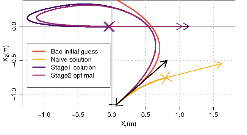
Figure 2: An example TOC-ORBA problem: solutions found by the different solvers, compared to the optimal and initial paths given a poor initial guess; arrows show direction and relative magnitude of final velocity.

IV-A Two-Stage Solver For TOC-ORBA

To avoid the problem of local minima, we split the solver into two stages: stage 1 holds $T$ constant at the computed upper bound (Section IV) and minimizes the cost function $F_{\mathrm{BV}}$; and stage 2 takes the parameter set found by stage 1 as an initial guess and minimizes $F_{\mathrm{BV}}$ further by allowing $T$ to vary. We call this solution the two-stage optimal control solver (TSOCS). Despite the fact that stage 1 is unlikely to find a valid solution, the parameter set found typically provides an initial guess to stage 2 within its optimal basin of attraction. Fig. 2 shows the paths corresponding to the local minimum and the global minimum found by TSOCS.

IV-B Iterative Closed-Loop Control

A real omnidirectional robot will have actuation errors, which will perturb it from the desired trajectory. To overcome such actuation errors, we present an iterative closed-loop controller using TSOCS, which re-solves the TOC-ORBA problem with new observations at every time-step.

Algorithm 1 lists IterativeTSOCS, which implements iterative closed-loop control using TSOCS. Given the desired final location and velocity ${\mathbf{x}}^{\mathcal{F}},{\mathbf{v}}^{\mathcal{F}}$, IterativeTSOCS first computes the initial guess to the optimal control parameters $\vec{\boldsymbol{\alpha}},T$ (line 3). Next, it executes the iterative control loop until the robot reaches the desired final location and velocity (line 4). At each time-step, IterativeTSOCS updates the current state of the robot based on new observations (line 18), and computes a new initial guess for the optimal control parameters by moving the initial adjoint point forward along the adjoint line (line 15–line 17) by the time-period $\Delta T$.

To prevent frequent backtracking due to small actuation errors, IterativeTSOCS runs an variant of the TSOCS second stage solver with a modified cost function $F_{\mathrm{it}}$,

$$F_{\mathrm{it}}= ||{\mathbf{x}}^{\mathcal{F}}-\mathbf{x}(T)||^{2}+\beta||{\mathbf{v}}^{\mathcal{F}}-\mathbf{v}(T)||^{2}+k_{1}e^{k_{2}(T/T_{e}-\tau)},$$

$$\beta= \max\left(1-\frac{||{\mathbf{v}}^{\mathcal{F}}-{\mathbf{v}}^{\mathcal{I}}||}{u_{\mathrm{max}}T_{e}},\beta_{\mathrm{min}}\right).$$ (17)

$F_{\mathrm{it}}$ modifies the boundary value cost function (Eq. IV) by including a regularization cost for the total time $T$, and a discount factor $\beta$ for the velocity error. The time regularization term, $k_{1}e^{k_{2}(T/T_{e}-\tau)}$, grows large if $T$ becomes more than $\tau$ times $T_{e}$, the expected time based off the previous iteration’s time. This prevents the robot from backtracking to correct for small actuation errors, which would take much more time that following the original trajectory. We chose $\tau=1.4$ in our experiments on real robots. The discount factor $\beta$ for the velocity error allows IterativeTSOCS to reach the final state with small errors in velocity while maintaining location accuracy, which would have been otherwise dynamically infeasible for the robot to correct without backtracking. $\beta$ decreases as the problem becomes near one-dimensional, because TSOCS fails on near one-dimensional cases more frequently.

If any iteration fails to find path using the paremeter guess from the updated adjoint line, then IterativeTSOCS runs the full two-stage solver on that iteration, with the second stage using the cost function in Eq. 17. If that fails as well, then IterativeTSOCS resorts to following open loop control from the last successful parameter set found.

Algorithm 1 Iterative TSOCS

1:procedure IterativeTSOCS(${\mathbf{x}}^{\mathcal{F}},{\mathbf{v}}^{\mathcal{F}}$)

2:    ${\mathbf{x}}^{\mathcal{I}},{\mathbf{v}}^{\mathcal{I}}\leftarrow$ Observe()

3:    $\langle\vec{\boldsymbol{\alpha}},T\rangle\leftarrow$ Stage1(${\mathbf{x}}^{\mathcal{I}},{\mathbf{v}}^{\mathcal{I}},{\mathbf{x}}^{\mathcal{F}},{\mathbf{v}}^{\mathcal{F}}$)

4:    while $||{\mathbf{x}}^{\mathcal{I}}-{\mathbf{x}}^{\mathcal{F}}||>\epsilon_{\mathbf{x}}\wedge||{\mathbf{v}}^{\mathcal{I}}-{\mathbf{v}}^{\mathcal{F}}||>\epsilon_{\mathbf{v}}\wedge T>\Delta T$ do

5:         $\langle\vec{\boldsymbol{\alpha}}_{\mathrm{n}},T_{\mathrm{n}},F_{\mathrm{it}}\rangle\leftarrow$ Stage2It(${\mathbf{x}}^{\mathcal{I}},{\mathbf{v}}^{\mathcal{I}},{\mathbf{x}}^{\mathcal{F}},{\mathbf{v}}^{\mathcal{F}},\vec{\boldsymbol{\alpha}},T$)

6:         if $F_{\mathrm{it}}<\epsilon_{\text{cost}}$ then

7:             $\langle\vec{\boldsymbol{\alpha}},T\rangle\leftarrow\langle\vec{\boldsymbol{\alpha}}_{\mathrm{n}},T_{\mathrm{n}}\rangle$

8:             $T\leftarrow T_{\mathrm{n}}$

9:         else

10:             $\langle\vec{\boldsymbol{\alpha}}_{\mathrm{n}},T_{\mathrm{n}}\rangle\leftarrow$ Stage1(${\mathbf{x}}^{\mathcal{I}},{\mathbf{v}}^{\mathcal{I}},{\mathbf{x}}^{\mathcal{F}},{\mathbf{v}}^{\mathcal{F}}$)

11:             $\langle\vec{\boldsymbol{\alpha}}_{\mathrm{n}},T_{\mathrm{n}},F_{\mathrm{it}}\rangle\leftarrow$ Stage2It(${\mathbf{x}}^{\mathcal{I}},{\mathbf{v}}^{\mathcal{I}},{\mathbf{x}}^{\mathcal{F}},{\mathbf{v}}^{\mathcal{F}},\vec{\boldsymbol{\alpha}},T$)

12:             if $F_{\mathrm{it}}<\epsilon_{\text{cost}}$ then

13:                 $\langle\vec{\boldsymbol{\alpha}},T\rangle\leftarrow\langle\vec{\boldsymbol{\alpha}}_{\mathrm{n}},T_{\mathrm{n}}\rangle$                       

14:         Execute($\vec{\boldsymbol{\alpha}}$)

15:         $\vec{\boldsymbol{\alpha}}.\alpha_{3}\leftarrow\vec{\boldsymbol{\alpha}}.\alpha_{3}+\vec{\boldsymbol{\alpha}}.\alpha_{1}\Delta T$

16:         $\vec{\boldsymbol{\alpha}}.\alpha_{4}\leftarrow\vec{\boldsymbol{\alpha}}.\alpha_{4}+\vec{\boldsymbol{\alpha}}.\alpha_{2}\Delta T$

17:         $T\leftarrow T-\Delta T$

18:         ${\mathbf{x}}^{\mathcal{I}},{\mathbf{v}}^{\mathcal{I}}\leftarrow$ Observe()     

After Stage2It recomputes the optimal control parameters $\vec{\boldsymbol{\alpha}}$ (line 5), the robot executes the control for the time-step according to the updated parameters $\vec{\boldsymbol{\alpha}}$ (line 14).

V Experimental Results

\begin{overpic}[width=433.62pt,unit=1mm]{true_path_zero.eps} \end{overpic}

(a) Zero final velocity

\begin{overpic}[width=433.62pt,unit=1mm]{true_path_nonzero.eps} \end{overpic}

(b) Non-zero final velocity

Figure 3: Examples of TSOCS and NTOC run on real robots. Yellow is the optimal path computed by TSOCS, blue is the path taken by real robots runnings TSOCS, and red is the path taken by real robots running NTOC.

We performed ablation tests in simulation to see how different parts of TSOCS affect its success rate. We also performed experiments in simulation and on real robots to evaluate 1) the execution times for TSOCS, 2) its accuracy at reaching final locations and velocities, and 3) the tradeoff between location and velocity accuracy for trajectories with non-zero final velocities. For the experiments with zero final velocities, we compared the results of TSOCS to NTOC.

TSOCS implementation

We implemented TSOCS in C++ using Ceres-Solver [19] as the nonlinear least-squares optimizer. Our implementation took an average of $0.38$\mathrm{ms}$$ to solve the TOC-ORBA problem for each iteration of closed loop control (Section IV-B), with some iterations taking as long as $9$\mathrm{ms}$$. The controller runs at $60$\mathrm{Hz}$$, so our implementation is able to execute within the timing constraints for real-time control.

Experiments in simulation

We simulated omnidirectional robots with actuation noise at every time step such that $v(t)=v_{u}(t)*\eta(1,n)$ where $v_{u}$ is the expected velocity from executing the control and $n$ is the noise level. TSOCS is run without regularization and with $\beta=1$ at all times in simulation. For comparing TSOCS to NTOC with problems with zero final velocity, we generated 10,000 random problems by sampling initial locations and velocities of the robot and setting the desired final location to the origin at rest. For evaluating the performance of TSOCS with problems with non-zero final velocities, we generated 10,000 problems by sampling initial locations and velocities, and setting the desired final location to the origin, with randomly sampled final velocities.

Experiments with real robots

We use four-wheeled omnidirectional robots designed for use in the RoboCup Small Size League [20]. For state estimation, we used SSL-Vision [21] with ceiling-mounted cameras to track the robots using colored markers, and performed state estimation with an extended Kalman filter. We limited the robots to a maximum of 2 m/s² acceleration.

We generated problems for real robots by starting the robot at the origin with randomly sampled initial velocities and final locations within a $2$\mathrm{m}$\times 2$\mathrm{m}$$ window of the starting location. We sampled 20 problems each with zero, and non-zero final velocities, and repeated each problem 5 times each, for a total of 100 trials for each condition on the real robot. We compared TSOCS and NTOC for the set of problems with zero final velocity, and evaluated TSOCS on the separate set of problems with nonzero final velocity, which NTOC cannot solve. We refer to TSOCS problems with zero final velocity as TSOCS-r.

V-A Ablation Tests

To compare how different features of TSOCS affect its success rate, we ran one million trials of the TSOCS solver on problems with nonzero final velocity. We performed one iteration of TSOCS per problem, rather than a full control sequence, to test the full two-stage solver. Table I shows the results without various features: $T_{\mathrm{max}}$ refers to the upper bound on travel time that stage 1 uses as an initial guess and holds constant. Without $T_{\mathrm{max}}$, we use $T=1$ for stage 1. Without the initial guess described in Section IV, we guess $\vec{\boldsymbol{\alpha}}=(1,2,3,4)$. Stage 1, along with the initial guess for $\vec{\boldsymbol{\alpha}}$ and $T$, both improve TSOCS’ success rate. TSOCS with the time upper bound, initial guess, and first stage (the configuration used on all subsequent experiments) can solve over 99% of problems.

Solution Method	Failure Rate
No $T_{\mathrm{max}}$, No Initial Guess, No Stage 1	30.49%
$T_{\mathrm{max}}$, No Initial Guess, No Stage 1	23.53%
No $T_{\mathrm{max}}$, No Initial Guess, Stage 1	9.76%
$T_{\mathrm{max}}$, Initial guess, No Stage 1	9.25%
$T_{\mathrm{max}}$, Initial Guess, Stage 1	0.39%

TABLE I: Impact of different steps on TSOCS failure rate.

V-B Accuracy in Travel Time

Control	Real Robots	Simulation
		No Noise	$5\%$ Noise
TSOCS	.13 [.09, .19]	0.00 [-0.01, 0.00]	0.09 [-0.09, 0.90]
TSOCS-r	.34 [.13, .57]	-0.01 [-0.01, 0.00]	0.07 [-0.12, 0.99]
NTOC	.33 [.15, .53]	0.00 [0.00, 0.05]	0.43 [0.00, 2.01]

TABLE II: Median $T_{\mathrm{rel}}$ with 95% confidence intervals.

To compare travel time accuracy between TSOCS and NTOC, we compared $T_{\mathrm{rel}}=\frac{T_{f}-T_{o}}{T_{o}}$, where $T_{f}$ is the actual time taken by the robot to reach its goal and $T_{o}$ is the optimal time for the problem. Table II shows the median and 95% confidence interval for $T_{\mathrm{rel}}$ for real and simulated robots.

In simulation without noise, iterative TSOCS and NTOC produce travel times that are close to optimal, as expected. With 5% simulated noise, both control algorithms take longer than the optimal time to execute, but TSOCS gets significantly closer to the optimal time than NTOC. For problems with non-zero final velocity and with 5% noise, TSOCS had a median execution error of $9\%$ of the optimal time.

On real robots, the effect of noisy actuation is much greater than that of 5% noise in simulation. TSOCS-r and NTOC both took around a third longer than optimal, partially because the robot could take extra time to reapproach the goal location if it overshot it. On TSOCS problems with nonzero final velocity, the robot could not reapproach the goal without incurring a large time penalty, which time regularization (Eq. 17) prevents, so the relative time of problems with nonzero final velocity was lower.

V-C Accuracy in Execution

We ran TSOCS and NTOC on the same problem conditions with zero final velocity, and separate TSOCS problems with nonzero final velocity that NTOC could not solve. We show examples of paths taken by TSOCS and NTOC alongside optimal paths in  Fig. 3. For problems with zero final velocity, TSOCS-r and NTOC had similar final location and velocity errors. All final location errors were less than $7$\mathrm{mm}$$, and all final velocity errors were less than $100$\mathrm{mm}\text{\,}{\mathrm{s}}^{-1}$$.

V-D Tradeoff Between Location and Velocity Error

In TSOCS problems with nonzero final velocity, there is a tradeoff between location accuracy and velocity accuracy. Unlike in problems with zero final velocity, if a robot overshoots its goal, it cannot immediately re-approach the final location without significant backtracking. Thus when a robot is perturbed slightly from its path and can no longer exactly acheive its goal location and velocity without backtracking, it must compromise by accepting either some location error or some velocity error. The $\beta_{\mathrm{min}}$ parameter of the iterative cost function in Eq. 17 controls that tradeoff.

Fig. 5 shows that increasing $\beta_{\mathrm{min}}$, which increases the weight given to the velocity error in the modified cost function in Eq. 17, increases location error and decreases velocity error, as expected. For $\beta_{\mathrm{min}}=0.01$, the final velocity errors were less than $0.16$\mathrm{m}\text{\,}{\mathrm{s}}^{-1}$$, and the final location errors less than $0.03$\mathrm{m}\text{\,}{\mathrm{s}}^{-1}$$ for all trials. We used $\beta_{\mathrm{min}}=0.01$ in all other experiments with TSOCS on real robots.

\begin{overpic}[width=433.62pt,unit=1mm]{error_histogram_location.eps} \end{overpic}

(c) Location errors.

\begin{overpic}[width=433.62pt,unit=1mm]{error_histogram_velocity.eps} \end{overpic}

(d) Velocity errors.

Figure 4: Distributions of TSOCS-r and NTOC errors in final location and velocity on real robots.

\begin{overpic}[width=433.62pt,unit=1mm]{xv_tradeoff_location.eps} \end{overpic}

(a) Location errors.

\begin{overpic}[width=433.62pt,unit=1mm]{xv_tradeoff_velocity.eps} \end{overpic}

(b) Velocity errors.

Figure 5: The tradeoff in location accuracy and velocity accuracy in problems with nonzero velocity on real robots.

VI Conclusion

We introduced a two-stage optimal control solver (TSOCS) to solve the time-optimal control problem for omnidirectional robots with bounded acceleration and unbounded velocity. TSOCS can exactly solve problems with both initial and final velocity, which were previously unsolvable. We demonstrated a closed loop real-time controller using TSOCS to control robots with noisy actuation in simulation, and on real robots.

References

- [1] J. Biswas and M. Veloso, “The 1,000-km challenge: Insights and quantitative and qualitative results,” IEEE Intelligent Systems , vol. 31, no. 3, pp. 86–96, 2016.
- [2] J. P. Mendoza, J. Biswas, P. Cooksey, R. Wang, S. Klee, D. Zhu, and M. Veloso, “Selectively reactive coordination for a team of robot soccer champions,” in AAAI Conference on Artificial Intelligence , 2016, pp. 3354–3360.
- [3] C. Röhrig, D. Heß, C. Kirsch, and F. Künemund, “Localization of an omnidirectional transport robot using IEEE 802.15. 4a ranging and laser range finder,” in IEEE/RSJ International Conference on Intelligent Robots and Systems, 2010, pp. 3798–3803.
- [4] F. G. Pin and S. M. Killough, “A new family of omnidirectional and holonomic wheeled platforms for mobile robots,” IEEE transactions on robotics and automation, vol. 10, no. 4, pp. 480–489, 1994.
- [5] T. Kalmár-Nagy, R. D’Andrea, and P. Ganguly, “Near-optimal dynamic trajectory generation and control of an omnidirectional vehicle,” Robotics and Autonomous Systems, vol. 46, no. 1, pp. 47–64, 2004.
- [6] W. Wang and D. J. Balkcom, “Analytical time-optimal trajectories for an omni-directional vehicle,” in IEEE International Conference on Robotics and Automation, 2012, pp. 4519–4524.
- [7] S. Pifko, A. Zorn, and M. West, “Geometric interpretation of adjoint equations in optimal low thrust trajectories,” Guidance, Navigation, and Control and Co-located Conferences, Aug 2008.
- [8] L. S. Pontryagin, Mathematical theory of optimal processes. CRC Press, 1987.
- [9] M. Renaud and J.-Y. Fourquet, “Minimum time motion of a mobile robot with two independent, acceleration-driven wheels,” in IEEE International Conference on Robotics and Automation, 1997, pp. 2608–2613.
- [10] M. Chyba and S. Sekhavat, “Time optimal paths for a mobile robot with one trailer,” in IEEE/RSJ International Conference on Intelligent Robots and Systems, vol. 3, 1999, pp. 1669–1674.
- [11] D. Verscheure, B. Demeulenaere, J. Swevers, J. De Schutter, and M. Diehl, “Time-optimal path tracking for robots: A convex optimization approach,” IEEE Transactions on Automatic Control, vol. 54, no. 10, pp. 2318–2327, 2009.
- [12] H. W. Kuhn and A. W. Tucker, “Nonlinear programming,” in Berkeley Symposium on Mathematical Statistics and Probability. Berkeley, Calif.: University of California Press, 1951, pp. 481–492.
- [13] A. M. Mohammed and S. Li, “Dynamic neural networks for kinematic redundancy resolution of parallel stewart platforms,” IEEE transactions on cybernetics, vol. 46, no. 7, pp. 1538–1550, 2016.
- [14] F. Altché, X. Qian, and A. de La Fortelle, “Time-optimal coordination of mobile robots along specified paths,” in IEEE/RSJ International Conference on Intelligent Robots and Systems, 2016, pp. 5020–5026.
- [15] M. Davoodi, F. Panahi, A. Mohades, and S. N. Hashemi, “Multi-objective path planning in discrete space,” Applied Soft Computing, vol. 13, no. 1, pp. 709–720, 2013.
- [16] X. Li and A. Zell, “Motion control of an omnidirectional mobile robot,” in Informatics in Control, Automation and Robotics. Springer, 2009, pp. 181–193.
- [17] O. Peñaloza-Mejía, L. A. Márquez-Martínez, J. Alvarez, M. G. Villarreal-Cervantes, and R. García-Hernández, “Motion control design for an omnidirectional mobile robot subject to velocity constraints,” Mathematical Problems in Engineering, vol. 2015, 2015.
- [18] D. J. Balkcom, P. A. Kavathekar, and M. T. Mason, “Time-optimal trajectories for an omni-directional vehicle,” The International Journal of Robotics Research, vol. 25, no. 10, pp. 985–999, 2006.
- [19] S. Agarwal, K. Mierle, and Others, “Ceres solver,” http://ceres-solver.org.
- [20] A. Weitzenfeld, J. Biswas, M. Akar, and K. Sukvichai, “Robocup small-size league: Past, present and future,” in Robot Soccer World Cup. Springer, 2014, pp. 611–623.
- [21] Zickler, Laue, G. Jr, Birbach, Biswas, and Veloso, “Five years of ssl-vision–impact and development,” in RoboCup 2013: Robot World Cup XVII. Springer Berlin Heidelberg, 2014, pp. 656–663.