The Discovery of a Gravitationally Lensed Supernova Ia at Redshift 2.22

Abstract

We present the discovery and measurements of a gravitationally lensed supernova (SN) behind the galaxy cluster MOO J1014+0038. Based on multi-band Hubble Space Telescope and Very Large Telescope (VLT) photometry of the supernova, and VLT spectroscopy of the host galaxy, we find a 97.5% probability that this SN is a SN Ia, and a 2.5% chance of a CC SN. Our typing algorithm combines the shape and color of the light curve with the expected rates of each SN type in the host galaxy. With a redshift of 2.2216, this is the highest redshift SN Ia discovered with a spectroscopic host-galaxy redshift. A further distinguishing feature is that the lensing cluster, at redshift 1.23, is the most distant to date to have an amplified SN. The SN lies in the middle of the color and light-curve shape distributions found at lower redshift, disfavoring strong evolution to $z=2.22$. We estimate an amplification due to gravitational lensing of $2.8^{+0.6}_{-0.5}$ ($1.10\pm 0.23$ mag)—compatible with the value estimated from the weak-lensing-derived mass and the mass-concentration relation from $\Lambda$CDM simulations—making it the most amplified SN Ia discovered behind a galaxy cluster.

1 Introduction

Gravitational lensing by massive galaxy clusters offers an amplified and magnified view of the high-redshift universe. Several examples of supernovae (SNe) lensed by foreground clusters have been found in recent years (Goobar et al., 2009; Amanullah et al., 2011; Nordin et al., 2014; Patel et al., 2014; Kelly et al., 2015; Rodney et al., 2015a; Petrushevska et al., 2016). Four of these cluster-lensed SNe have been of Type Ia (SNe Ia), from which the amplification due to lensing has been determined. (Two additional SNe Ia that were lensed by field galaxies have also been found, Quimby et al. 2014; Goobar et al. 2017; we summarize all referenced SNe in Table 1).

The uniquely precise standardization possible with SNe Ia provides amplification information, breaking the so-called mass-sheet degeneracy that is problematic for most shear-based lensing models, and permits independent direct tests of cluster mass models obtained from galaxy lensing (Nordin et al., 2014; Patel et al., 2014; Rodney et al., 2015a). Lenses that produce multiple SN images provide additional model constraints (Kelly et al., 2016a). To date the redshifts of gravitationally lensed background SNe Ia have been at $z<1.39$, a redshift range where even without lensing the complete (normal) SN Ia population can be detected using single-orbit HST visits. In cases of stronger amplification of sources beyond the redshift reach of normal observations, tests of SN Ia properties and rates over a larger look-back time become possible. Here we report the discovery of the most amplified SN Ia behind a galaxy cluster ever found, with a spectroscopic host-galaxy redshift making it also the most distant.

Table 1: Other high-redshift or gravitationally lensed SNe.

SN	Redshift	Redshift Type	Lens	Lens Redshift	Amplification	Type	Reference
CAND-ISAAC	0.64	Spec	Cluster	0.18	3.6	IIP	Goobar et al. (2009); Stanishev et al. (2009)
PS1-10afx	1.39	Spec	Field	1.12	30	Ia	Quimby et al. (2014)
A1, CLA11Tib	1.14	Spec	Cluster	0.19	1.4	Ia	Nordin et al. (2014); Patel et al. (2014)
H1, CLN12Did	0.85	Spec	Cluster	0.35	1.3	Ia	Nordin et al. (2014); Patel et al. (2014)
L2, CLO12Car	1.28	Spec	Cluster	0.39	1.7	Ia	Nordin et al. (2014); Patel et al. (2014)
Refsdal	1.49	Spec	Cluster	0.54	$\sim 100$	II	Kelly et al. (2015, 2016b)
HFF14Tom	1.35	Spec	Cluster	0.31	1.7	Ia	Rodney et al. (2015a)
GND13Sto	$1.80\pm 0.02$	Phot	$\cdots$	$\cdots$	$\cdots$	Ia	Rodney et al. (2015b)
GND12Col	$2.26^{+0.02}_{-0.10}$	Phot	$\cdots$	$\cdots$	$\cdots$	Ia	Rodney et al. (2015b)
CAND-669	0.67	Spec	Cluster	0.18	1.3	IIL	Petrushevska et al. (2016)
CAND-821	1.70	Spec	Cluster	0.18	4.3	IIn	Amanullah et al. (2011); Petrushevska et al. (2016)
CAND-1392	0.94	Spec	Cluster	0.18	2.7	IIP	Petrushevska et al. (2016)
CAND-10658	$0.94^{+0.07}_{-0.27}$	Spec	Cluster	0.18	1.7	IIn	Petrushevska et al. (2016)
CAND-10662	$1.03^{+0.20}_{-0.17}$	Spec	Cluster	0.18	2.6	IIP	Petrushevska et al. (2016)
iPTF16geu	0.41	Spec	Field	0.22	52	Ia	Goobar et al. (2017)
SCP16C03 (“Joseph”)	2.22	Spec	Cluster	1.23	2.8	Ia	This Work

2 Discovery

The Supernova Cosmology Project’s “See Change” program (PI: Perlmutter) monitored twelve massive galaxy clusters in the redshift range 1.13 to 1.75 using the Hubble Space Telescope (HST) Wide Field Camera 3 (WFC3) with the goals of greatly expanding the range of the high-redshift SN Ia Hubble diagram and accurately determining high-redshift cluster masses via weak lensing. We observed each cluster every 5 weeks for one orbit split between the UVIS $F814W$, the IR $F105W$, and the IR $F140W$ filters. The supernova survey was very deep; our 50% completeness for simulated SN detection was AB 26.6 in $F105W+F140W$ (Hayden et al., in prep.); this is $\sim 1$ magnitude fainter than a $z=1.75$ SN Ia at maximum. When a promising Type Ia supernova candidate was found, at least one extra visit was triggered and executed within 2–3 observer frame weeks after the initial discovery. These extra visits provided better light-curve sampling, usually close to maximum light, and frequently extended the wavelength range with the IR $F160W$ filter.

On 2016 Feb 29 UTC, we searched images of the WISE-selected (Wright et al., 2010) massive galaxy cluster MOO J1014+0038 ($z=1.23$, Decker et al. in prep.; $M_{200}=(5.6\pm 0.6)\times 10^{14}M_{\odot}$, Brodwin et al. 2015), from the Massive and Distant Clusters of WISE Survey (MaDCoWS; Gettings et al. 2012, Stanford et al. 2014, Gonzalez et al. 2015). We detected a red (WFC3 $F140W=25.1$, $F105W-F140W=1.4$ AB mag; upper limit only in $F814W$) supernova at $\alpha=153\fdg 52655$, $\delta=+0\fdg 64041$ (J2000, aligned to USNO-B1). This SN was internally designated as SN SCP16C03, as it was the third SN found in this cluster field (alphabetically labeled cluster “C”) in 2016. As shown in Figure 1, the SN lies on a red galaxy having a color of $F105W-F140W=1.5$ AB mag and is located 0$\farcs$7 from the core of this galaxy ($\alpha=153\fdg 52643$, $\delta=+0\fdg 64025$). We conclude that this galaxy must be the host galaxy; there are no other galaxies nearby, the light curve is incompatible with those possible from an intra-cluster SN within MOO J1014+0038 (as discussed in Section 6), and the probability of a chance projection is negligible ($\sim 0.2$%, as discussed in Appendix B).

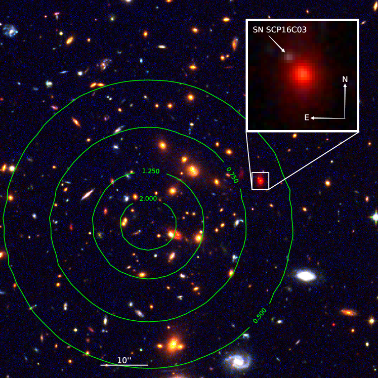
Figure 1: Color image of the central part of MOO J1014+0038 made with an $F814W$ stack and the $F105W$ and $F160W$ data from our first triggered HST imaging near maximum light. The inset panel uses different scaling, and incorporates only IR data ($F105W$, $F125W$, and $F160W$). The compass arrows are 1″ in linear scale. Both panels use hyperbolic arcsine intensity scaling. In green, we show contours of our computed lensing amplification model (in magnitudes), described in Section 8.

3 Spectroscopic and Photometric Follow-up

We activated ToO spectroscopic observations (PI: Hook) using X-shooter, the multi-wavelength medium resolution spectrograph on the Very Large Telescope (Vernet et al., 2011). Five “Observation Blocks” were taken between 2016 Mar 4-5 (UT), yielding a total integration time of 3.8, 4.4, and 5.0 hours in the X-shooter UVB, VIS, and NIR arms, respectively. Although the slit orientation captured both the host galaxy and the SN (shown in Figure 2), the galaxy was $\sim 4$ magnitudes brighter so only a host-galaxy spectrum could be extracted. The data were reduced to wavelength- and flux-calibrated, sky-subtracted, 2D spectra using the Reflex software (Freudling et al., 2013). Optimal 1D-extractions were determined using a combination of custom and IRAF (Tody, 1993) routines. The extractions used a Gaussian profile in the cross-dispersion direction, the width of which was determined by fitting the trace in each (binned) 2d spectrum individually. These extractions were combined using the weighted mean to create a final 1D spectrum. We corrected for telluric absorption using a model atmosphere computed by the Line-By-Line Radiative Transfer Model (Clough et al., 1992, 2005) retrieved through Telfit (Gullikson et al., 2014). Our observations were obtained at a low mean airmass of $\sim 1.15$ with a NIR slit width of $0\farcs 9$ (matching the mean seeing). The X-shooter NIR arm is aligned with the optical at 13,100 Å; the atmospheric differential refraction over the NIR wavelength range for this airmass range is $<0\farcs 1$. For a Gaussian PSF (with FWHM $0\farcs 9$) shifted by $0\farcs 1$, the differential slit loss would be $2\%$. Thus, atmospheric differential refraction has a negligible impact on the calibration of our NIR spectrum. The host-galaxy spectrum is shown in Figure 3. Balmer H$\delta$ and H$\beta$ absorption lines are clearly detected, as are the Ca H&K absorption lines. Mg b is likely detected as well. These lines provide the main contribution to the weighted cross-correlation, as shown in the lower panel of Figure 3, yielding a redshift of $2.2216\pm 0.0002$ for the host galaxy. No emission lines were detected (see Section 5.3 for further details).

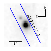
Figure 2: Illustration of the X-shooter slit orientation and location on the SN and host galaxy.

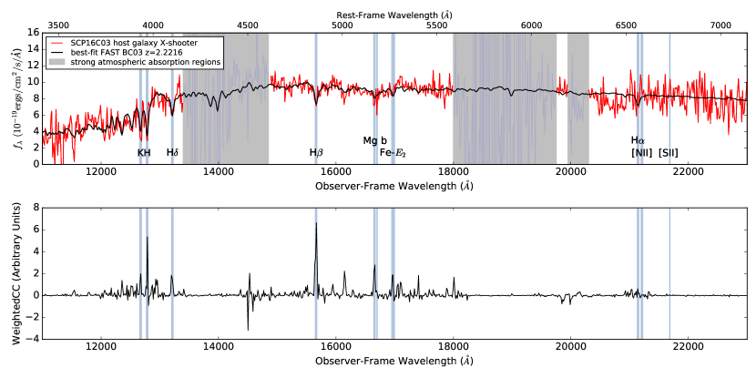
Figure 3: Top: Flux-calibrated, telluric corrected, de-lensed (by a factor of 2.8; see Section 7) and binned (14Å observer-frame) spectrum of the host galaxy (red line). Gray shaded regions indicate strong atmospheric absorption. The best-fit FAST model (fit to both the photometry and spectrum) is shown in black, convolved by the 305 km/s velocity dispersion estimated by ppxf. Prominent features identified in both spectra are highlighted with light blue shading, and labeled; the H$\alpha$ line is labeled for reference, but no prominent contribution to the cross-correlation is detected from it. Bottom: The contribution to the weighted cross-correlation of each wavelength element of the spectrum. Regions of heavy atmospheric absorption are properly de-weighted, and the prominent features easily identified by eye provide a confident redshift determination of $2.2216\pm 0.0002$.

This SN was 15″ away from the center of a dense concentration of cluster galaxies. Our initial flux amplification estimate was $\sim 2.2$, calculated by assuming that the optical and halo center were the same, and employing a Navarro-Frenk-White dark matter profile (Navarro et al., 1997). Based on the likelihood that this would turn out to be a highly magnified, high-redshift SN Ia, we applied for Director’s Discretionary time on HST and were granted a three-orbit disruptive ToO to ensure a good measurement of the SN SED. We triggered $F105W$, $F125W$, and $F160W$ imaging from our “See Change” allocation. We did not request HST grism spectroscopy, as the roll angle range available would not have allowed for a clean separation of the SN and its host. In addition to our triggered followup, we obtained additional WFC3 $F814W$, $F105W$, and $F140W$ imaging at two more previously scheduled orbits (the cadenced search visits for discovering SNe). We also were granted Director’s Discretionary time on VLT for imaging in the $K_{s}$ band (PI: Nordin) with HAWK-I (Kissler-Patig et al., 2008) in order to extend the wavelength range redder than is possible with HST.

4 SN Photometry

With a pixel size of $\sim 0\farcs 128$, the WFC3 IR channel undersamples the PSF, making it difficult to remove underlying galaxy light with image resampling and subtraction. In addition, this SN poses a (unusual, but not unknown) challenge, as we have no reference (SN-free) images in $F125W$ and $F160W$, necessitating interpolation of the galaxy light over the SN position. To meet these needs, we have developed a “forward modeling” code described in Suzuki et al. (2012) and Rubin et al. (2013) and updated for WFC3 IR in Nordin et al. (2014). This code fits each pixel as observed (flat-fielded “flt” images for WFC3 IR, CTE-corrected, flat-fielded “flc” images for WFC3 UVIS), i.e., without resampling due to spatial alignment or correction for distortion. It does this by creating an analytic model of the scene, convolving that model with the PSF, and fitting it to the pixel values. In all cases, the effect on the flatfield of pixel area variations over the FoV are taken into account in order to properly account for spatial distortion.

For the host-galaxy, our analytic model is a linear sum of an azimuthally symmetric spline (a 1D, radially varying component that is allowed to have ellipticity) and a 2D grid to capture azimuthal asymmetries. To these splines, we include a model for a point source representing the SN, with a different fitted amplitude in each epoch. As there are reference images in the cadenced IR filters ($F105W$ and $F140W$), these can be used as a cross-check of our ability to do photometry in $F125W$ and $F160W$, for which references are lacking. We obtain nearly identical photometry in the $F105W$ and $F140W$ bands with and without modeling the reference images, although the uncertainties are smaller when including references. Testing with simulated SNe indicates no photometric biases at the 0.01 magnitude level, and accurate uncertainties, even without using reference images.

There is only weak evidence for SN light in the $F814W$ filter, as expected for such a high redshift SN Ia. The low S/N necessitates a different treatment than the IR, where the offset between the SN and host galaxy was treated as a fit parameter. To determine the location of the SN in the $F814W$ images, we start by aligning the UVIS and IR exposures using TweakReg, and then drizzling to a common frame using AstroDrizzle. (These resampled images are not used for the SN photometry.) Then we perform PSF photometry on the UVIS images using the centroid transferred (using pixtopix) from that measured in the IR images, where the SN is detected. We fit for a spatially constant background underneath the SN, incorporating both sky and underlying galaxy. Even the core of the galaxy is only detected at low S/N in each $F814W$ exposure, so the second derivative underneath the SN is small.

Bad weather allowed only one of the seven Hawk-I $K_{s}$ observing blocks to be executed; 40 minutes of effective exposure time was obtained in excellent seeing (0$\farcs$27) enabling a measurement of the SN flux. We use the same host-galaxy model as for the WFC3 IR data, but with the offset of the SN from the host fixed, and employing field stars to derive the PSF. We determine the flux calibration (in AB mags) from the standard star FS19 and from the 2MASS (Skrutskie et al., 2006) magnitudes of the field stars. Although the brightness uncertainty of 60% is too large to improve the distance measurements, the additional rest-frame $R$-band coverage helped with photometric classification.

We present the resulting SN photometry in Table 2. The uncertainty in the host-galaxy subtraction in each band leads to correlations between the WFC3 IR photometry measurements (in the data for each filter), so we also provide the inverse covariance matrix in Table 3. We take the WFC3 IR zeropoints from Nordin et al. (2014), converted to AB magnitudes, which take into account the WFC3 IR count-rate nonlinearity. For the UVIS F814W filter, we use the STScI-provided UVIS zeropoint, after correcting the encircled energy to an infinite aperture.

Table 2: Photometry for SN SCP16C03.

MJD	UT	Observation	Flux (e-/s)	Uncertainty	Chip	AB Zeropoint
HST $F814W$
57414.741	01-27-2016	Cadenced	0.162	0.079	2	25.146
57446.809	02-28-2016	Cadenced	0.079	0.070	1	25.146
57479.413	04-01-2016	Cadenced	0.056	0.071	2	25.146
57513.068	05-05-2016	Cadenced	0.000	0.066	1	25.146
VLT $K_{s}$
57479.051	04-01-2016	Triggered	173	102	3	30.26
HST $F105W$
57414.751	01-27-2016	Cadenced	0.095	0.145	1	26.235
57446.824	02-28-2016	Cadenced	0.779	0.197	1	26.235
57465.544	03-18-2016	Triggered	1.543	0.094	1	26.235
57479.426	04-01-2016	Cadenced	1.542	0.161	1	26.235
57513.081	05-05-2016	Cadenced	0.483	0.156	1	26.235
HST $F125W$
57462.864	03-15-2016	Triggered	3.205	0.172	1	26.210
57465.506	03-18-2016	Triggered	3.351	0.173	1	26.210
HST $F140W$
57414.756	01-27-2016	Cadenced	0.363	0.161	1	26.437
57446.820	02-28-2016	Cadenced	3.294	0.245	1	26.437
57479.413	04-01-2016	Cadenced	4.835	0.213	1	26.437
57513.068	05-05-2016	Cadenced	2.396	0.220	1	26.437
HST $F160W$
57462.909	03-15-2016	Triggered	2.673	0.176	1	25.921
57465.572	03-18-2016	Triggered	2.691	0.182	1	25.921

Note. — Photometry measured for each band on each date. Table 3 has the weight matrices for the WFC3 IR measurements.

Table 3: Inverse covariance matrices for the WFC3 IR photometry.

MJD	Inverse Covariance Matrix
$F105W$
57414.751	$48.2472$	$-1.2956$	$-5.6335$	$-1.7874$	-1.8504
57446.824	$-1.2956$	$26.0744$	$-3.3404$	$-1.0842$	-1.1516
57465.544	$-5.6335$	$-3.3404$	$115.3885$	$-4.6158$	-4.7575
57479.426	$-1.7874$	$-1.0842$	$-4.6158$	$39.0092$	-1.5386
57513.081	$-1.8504$	$-1.1516$	$-4.7575$	$-1.5386$	41.7656
$F125W$
57462.864	$35.4715$	$-7.4421$	$\cdots$	$\cdots$	$\cdots$
57465.506	$-7.4421$	$35.0010$	$\cdots$	$\cdots$	$\cdots$
$F140W$
57414.756	$39.2367$	$-1.5114$	$-1.8203$	$-1.8066$	$\cdots$
57446.820	$-1.5114$	$16.7848$	$-0.7807$	$-0.9239$	$\cdots$
57479.413	$-1.8203$	$-0.7807$	$22.1654$	$-1.0547$	$\cdots$
57513.068	$-1.8066$	$-0.9239$	$-1.0547$	$20.8010$	$\cdots$
$F160W$
57462.909	$34.5919$	$-8.5948$	$\cdots$	$\cdots$	$\cdots$
57465.572	$-8.5948$	$32.1690$	$\cdots$	$\cdots$	$\cdots$

Note. — Inverse covariance matrices for the WFC3 IR photometric measurements. These data are correlated (within each band) due to uncertainty in the underlying host-galaxy light.

5 Host Galaxy Properties

In this section, we present our measurements of the host-galaxy properties from spectroscopy and imaging, and summarize the evidence that the galaxy is old for its redshift and therefore lacking significant star formation in Section 5.5.

5.1 Host-galaxy Photometry

We perform photometry of the host galaxy on aligned, stacked (SN-free) images using SEP To minimize contamination by light from the nearby galaxies, we use an elliptical aperture set to 1.2 times the Kron radius (Kron, 1980). In addition to the HST WFC3 photometry, we use archival Spitzer IRAC CH1 and CH2 data (Gonzalez et al., in prep.), and we obtained bluer $g^{\prime}$, $r^{\prime}$ and $i^{\prime}$ photometry of the host with the OSIRIS instrument at the Gran Telescopio Canarias (GTC). We determine the zeropoints of this photometry using an SDSS star in the GTC field of view (both the star and galaxy are measured with the same elliptical aperture). We present the host-galaxy photometry in Table 4.

Table 4: Host-galaxy photometry.

Instrument	Filter	Flux ($\mu$Jy)	Flux Uncertainty ($\mu$Jy)
OSIRIS	$g^{\prime}$	0.19	0.03
OSIRIS	$r^{\prime}$	0.37	0.06
OSIRIS	$i^{\prime}$	0.55	0.10
WFC3	$F814W$	1.06	0.20
WFC3	$F105W$	3.66	0.08
WFC3	$F125W$	8.72	0.32
WFC3	$F140W$	15.05	0.08
WFC3	$F160W$	20.79	0.44
Hawk-I	$K_{s}$	32.09	1.12
IRAC	CH1	57.1	1.7
IRAC	CH2	63.8	1.7

Note. — Measured host-galaxy fluxes in the HST and GTC imaging. We scale to $\mu$Jy (AB zeropoint of 23.9).

5.2 Host Age, Star-formation Rate, and Mass from SED Fitting

While SED fitting to broadband photometry has a well-known degeneracy between age, dust, and metallicity (e.g. Bell & de Jong, 2001), the X-shooter spectrum has many absorption features that can help break that degeneracy. To simultaneously fit the spectrum and the photometry, we use FAST (Kriek et al., 2009).

We calibrate the X-shooter spectrum to the de-lensed HST photometry in bands $F125W$, $F140W$, and $F160W$ by integrating the de-lensed X-shooter spectrum over these filters; we find a multiplicative factor of 1.5 in flux is required to match the HST photometry. We then bin the X-shooter spectrum to 5 Å. We use the high-resolution stellar population synthesis models included with FAST, performing a fit using both Bruzual & Charlot 2003 (BC03) and Conroy et al. 2009 (FSPS) models, and averaging the two results (they agree extremely well). We use the Chabrier IMF (Chabrier, 2003), with a delayed-exponential star-formation history and the default ‘kc’ parameterization of the dust attenuation curve (Kriek & Conroy, 2013). We first fit to a coarse grid, then progressively fit to a finer grid near the best-fit region of parameter space to better estimate uncertainties. Note that FAST does not model emission lines. FAST returns a $\chi^{2}$ of 1385 for 2182 degrees of freedom for the BC03 models, and $\chi^{2}$ of 1414 for 2179 degrees of freedom using the FSPS models. The final uncertainties are estimated using the FAST Monte Carlo simulation option, sampling 1000 times. The best-fit model and derived parameters are presented in Table 5 and the model spectrum is shown overlaid on the X-shooter spectrum in Figure 3. The best-fit composite-stellar-population template has an age of $1.60\pm 0.1$ Gyr; as the age of the universe at $z=2.22$ is only 2.96 Gyr, the implied formation redshift is $z_{\mathrm{form}}\sim 4.5$. The galaxy is very massive, with a stellar mass of $11.08\pm 0.02$ M_⊙, and it has a low SFR of $0.4\pm 0.2$ M_⊙/yr (averaged over the prior 30 Myr) given its mass. The FAST star-formation history model indicates that 99.94% of all stars expected to ever form have already formed in this galaxy. FAST finds little dust, with a mean $A_{V}=$ $0.3\pm 0.08$. We assume a two-component dust model of Charlot & Fall (2000) where the dust optical depth for older stars is 0.3 times the optical depth for young (i.e., $<10$ Myr) stars. This implies $A_{V}\sim 1.0\pm 0.27$ mag for any young stellar component. The age measurement is sufficiently precise to contribute a cosmochronometry measurement and thereby help constrain cosmological parameters (e.g., Jimenez & Loeb, 2002; Stern et al., 2010; Moresco et al., 2012).

5.3 Emission-line measurement of the Star-Formation Rate

We measure equivalent widths from the spectral extractions centered on the core of the galaxy (shown in Figure 4). The region around [OII] and H$\alpha$ are modeled with the sum of the best-FIT FAST SED model (convolved to the ppxf velocity dispersion of 305 km/s) and Gaussian emission. We fix the emission component to have a velocity dispersion of 305 km/s. For [OII], we use two Gaussians, with the relative amplitude fixed to 0.74 for the $3726$Å component and 0.26 for the $3729$Å one.

We find a [OII] $\lambda 3727$ Å rest-frame equivalent width of $\textrm{EW([OII])}=1.5^{+3.0}_{-2.8}$ Å, as shown in Figure 4. We see no evidence of [OIII] $\lambda 5007$ Å emission; a nearby strong night sky line residual prevents us from measuring this spectral region. After correcting for the stellar Balmer absorption predicted by the FAST SED fit, we measure H$\alpha$ having EW(H$\alpha$) $=1.1^{+1.9}_{-1.7}$ Å. These weak emission line equivalent widths point to a low SFR per unit stellar mass.

Using the X-Shooter calibration discussed in Section 5.2, and correcting for extinction, we convert our H$\alpha$ equivalent width to a line luminosity of $L(\mathrm{H}\alpha)=2.4^{+4.1}_{-3.7}\times 10^{41}$ ergs/s. We then convert to a star formation rate using $\dot{\mathrm{M}}=5.45\times 10^{-42}\,L(\textrm{H}\alpha)$ (M_⊙/yr)/(erg/s) from Calzetti et al. (2010), resulting in $\dot{M}=1.3^{+2.3}_{-2.0}$ M_⊙/yr. The H$\alpha$ and SED-fit star-formation rates agree well, within $0.4\,\sigma$. At low SFR, OII emission can be badly contaminated by emission from post-AGB stars (e.g., Belfiore et al., 2016). If there were no such contamination, the derived SFR would be $9^{+20}_{-17}$ (M_⊙/yr)/(erg/s), using the conversion $\dot{M}=2.65\times 10^{-41}\,L(\textrm{OII})$ (Meyers et al., 2012) and our FAST SED extinction-corrected [OII] $\lambda 3727$ Å luminosity of L([OII]) $3.3^{+7.6}_{-6.2}\times 10^{41}$ M_⊙/yr)/(erg/s). This SFR estimate is consistent with the others (although with much larger uncertainties). However, we do not use it to estimate the SFR for this host. Likewise, while [OIII] $\lambda 5007$ Å is usually present when there is star formation, it is a poor SFR indicator due to its strong dependence on metallicity and the hardness of the stellar UV spectrum.

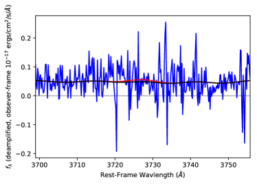
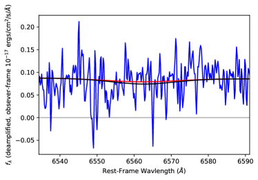
Figure 4: In blue, we show cutouts of the spectral regions for [OII] (left panel) and H$\alpha$ (right panel). No emission lines are detected in either region. In black, we show the best-fit FAST template, convolved to the ppxf velocity dispersion of 305 km/s. In red, we show the best-fit [OII] (left panel) and H$\alpha$ (right panel) contribution.

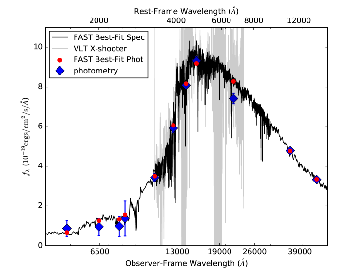
Figure 5: Host galaxy photometry and spectrum with the best-fit FAST model. The HST photometry was used for flux calibration of the X-shooter spectrum. The best-fit FAST model for both BC03 and FSPS templates is a massive galaxy with low SFR $0.4\pm 0.2$ M_⊙/yr. The age, SFR timescale parameter $\tau$, and rest-frame $U-V$ and $V-J$ colors (well-constrained by the GTC, HST, and Spitzer photometry) all imply a quiescent galaxy; with an age that is 10 times the e-folding timescale of the best fit stellar population model, 99.94% of stars expected to ever form in this galaxy have already formed.

Table 5: SCP16C03 Host-galaxy Properties

Quantity	Value	Notes
EW(OII 3727) (Å)	$1.5^{+3.0}_{-2.8}$
EW(H$\alpha$) (Å)	$1.1^{+1.9}_{-1.7}$	corrected for stellar absorption
Emission line SFR (M⊙/yr)	$1.3^{+2.3}_{-2.0}$	corrected for FAST $A_{V}$
Galaxy SED SFR (M⊙/yr)	$0.4\pm 0.2$	from FAST SED fit – integrated over past 30 Myr
$\log_{10}$(M/M⊙)	$11.08\pm 0.02$	from FAST SED fit
$\log_{10}$(Specific SFR (1/yr))	$-11.48^{+0.17}_{-0.30}$	derived from best-fit FAST SED
age (Gyr)	$1.60\pm 0.1$	age of universe $2.96$ Gyr at $z=2.2216$
$\tau$ (Gyr)	$0.16\pm 0.02$	SFR $\propto$ $t$e-t/τ
$A_{V}$	$0.3\pm 0.08$	using ‘kc’ dust parametrization in FAST
$(U-V)_{\mathrm{AB}}$	1.74	rest-frame $U-V$ derived from best-fit FAST SED
$(V-J)_{\mathrm{AB}}$	0.9	rest-frame $V-J$ derived from best-fit FAST SED
$\sigma$ (km/s)	$305\pm 42$	velocity dispersion measured with ppxf
$n$	$2.8\pm 0.1$	Sérsic index from forward model
reff (arcsec)	$0\farcs 225\pm 0.006$	half-light radius from raw pixels; not de-magnified
reff (kpc, de-mag)	$0.679\pm 0.017$	half-light radius in kpc, de-magnified by 2.8$\times$
log${}_{10}\Sigma$ (M${}_{\odot}/\mathrm{kpc}^{2}$)	$10.62\pm 0.02$	derived compactness

5.4 Profile Fitting

We also measure the surface brightness profile of the host galaxy. We fit the $F140W$ imaging, as it is close to rest-frame $B$-band. To determine the central profile given the undersampled imaging, we again use a forward-model approach. We model the observed pixels (without resampling) of nine dithers (from SN-free epochs) with a Sérsic profile (Sérsic, 1963) convolved with the PSF (the same PSF as for the SN photometry). We marginalize over the amplitude, half-light radius, ellipticity, and orientation. The galaxy is fit well by this simple model, with no evidence of an on-core point source (or variability) which might imply a central AGN (see Figure 6). We find a Sérsic index of $2.8\pm 0.1$, and a de-magnified half-light radius of $0.679\pm 0.017$ kpc. In combination with the total stellar mass, this implies central density of log${}_{10}\Sigma$ (M${}_{\odot}/\mathrm{kpc}^{2}$) = $10.62\pm 0.02$, as summarized in Table 5.

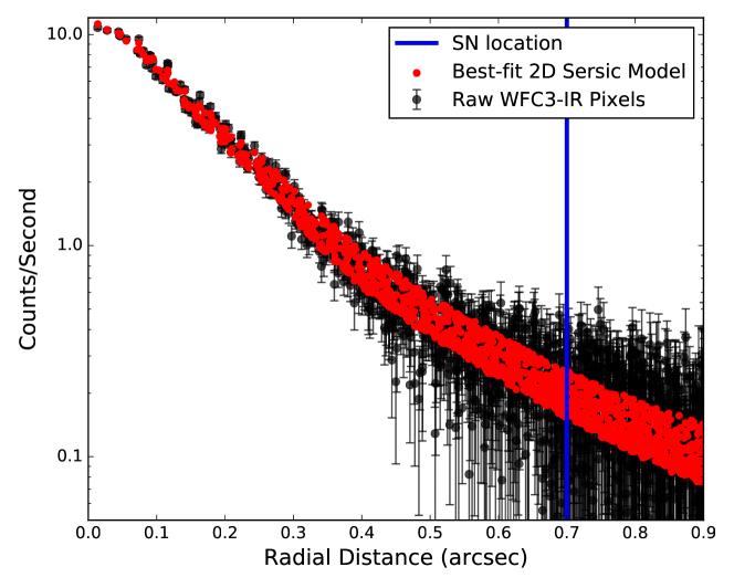
Figure 6: The radial brightness profile of the host galaxy (black points), with the best-fit 2D Sérsic model (red points). The scatter in the best-fit Sérsic model is a combination of the elliptical galaxy plotted in radial coordinates, and the asymmetric WFC3 IR PSF. The galaxy is well-fit by the 2D Sérsic profile, with a best-fit Sérsic index of $2.8\pm 0.1$ and a half-light radius of $0\farcs 225\pm 0.006$. The galactocentric radius at which the SN occurred is indicated by a vertical blue line at $0\farcs 7$.

5.5 Host Galaxy Summary

All host parameters point to the host galaxy being a massive quiescent galaxy. The velocity dispersion from the spectrum and the stellar mass from SED fitting provide joint confirmation of a high mass, while the SED fit to the spectrum and photometry provides a strong constraint on low SFR, reinforced by lack of evidence for emission lines in the spectrum. The derived specific SFR of log${}_{10}(\mathrm{sSFR})=-11.48^{+0.17}_{-0.30}$ qualifies this galaxy as being in a stage of quiescent star-formation, as defined by the mass-doubling criterion of Feulner et al. (2005) or the log${}_{10}(\mathrm{sSFR})<-11$ criterion of Domínguez Sánchez et al. (2011). The 10 star-formation $e$-folding times that have passed reinforces this conclusion. The structure of the host galaxy – its moderately high Sérsic index, small $r_{\mathrm{eff}}$, and high central density – is also consistent with other massive quiescent galaxies found at similar redshifts (Muzzin et al., 2012; van der Wel et al., 2014; Newman et al., 2015; van Dokkum et al., 2015; Barro et al., 2017).

At these high-redshifts it has become standard practice to define quiescence photometrically, based on the statistical separation of galaxies in rest-frame $U-V$ versus $V-J$ (the $UVJ$ diagram; Williams et al., 2009; Brammer et al., 2011) into a red, dead “clump” and a star-forming “track” derived using the UV$+$IR SFR. Spectroscopic follow-up has confirmed that the $UVJ$ diagram selects older, quiescent galaxies efficiently (Whitaker et al., 2013). In this space, dusty star-forming galaxies move along a track that is perpendicular to the separation between the quiescent clump and the star-forming track (Williams et al., 2009; Brammer et al., 2011). Movement from the star-forming track to the quiescent clump is well-described by passive stellar evolution (Williams et al., 2009). The unpopulated region between the quiescent clump and the star-forming track is known as the the “green valley”; it is not yet established whether these galaxies represent a short-lived (and dusty) evolutionary path from the star-formation main sequence to the red sequence of galaxies, or are merely the overlapping tails of two distinct populations with measurement scatter (see e.g. Pandya et al., 2017, for a review). Regardless, the $U-V$ and $V-J$ colors of the galaxy place it firmly in the quiescent regime according to the $UVJ$ classification scheme (see Table 5 and e.g. Brammer et al. 2011).

The lack of emission lines that trace star-formation, the low specific SFR and stellar extinction, the red color of the SED from rest-frame $U$ to $J$, and estimates of morphology from the imaging combine to strongly imply a quiescent galaxy, and not a dusty star-forming galaxy. Of course very sharp-edged dust structures, such that the affected stars contribute negligibly to the light and associated extinction we do detect, could hide more stellar mass and star formation. Such dust would also be required to preserve the smooth structure of this galaxy. In this particular case, such a contrived means of hiding significant stellar mass is especially unlikely since this galaxy is already on the steeply falling segment of the galaxy luminosity function. For instance, if half the stellar mass were hidden, the $2.0<z<2.5$ galaxy luminosity function (e.g. Davidzon et al., 2017) predicts a $65\times$ lower incidence per unit volume for the resulting galaxy. We also cannot rule-out a situation in which the specific line of sight for this SN has much less dust, thereby escaping these constraints from host galaxy properties. But such a finely-tuned case seems unlikely, and is unnecessary to explain our observations, as the following section will make apparent.

6 SN Photometric Classification

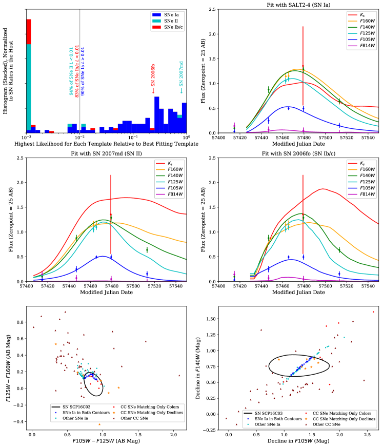
Figure 7: Top left panel: histogram of relative likelihoods from the light curve fits to the templates of each type of SN. The likelihoods are scaled so that the template with the highest likelihood has a value of 1. The histogram is normalized such that the area for each type of SN matches the relative rates expected in this galaxy (Section 6). This histogram indicates that, although there are two CC templates with a reasonable fit to the light curves, there are many more that are poor fits and thus the probability that SN SCP16C03 is a SN Ia is high. Light-curve panels: the best-fit for the SN Ia templates (top right), the SN II templates (middle left), and the SN Ib/c templates (middle right). In the bottom panels, we show how SN SCP16C03 compares to the template library in both color (bottom left: the $F105W-F125W$ and $F125W-F160W$ colors at the epoch with all three) and decline rate (bottom right: the decline between the last two epochs in $F105W$ and $F140W$). Each point plotted is from the best-fit (i.e., best-fit amplitude, date of maximum, and extinction) of one of the SN templates (for display purposes, we show as many SNe Ia realizations as CC templates, although most SNe in the host galaxy are SNe Ia). The black contours show the 68% confidence intervals from our measurements of SN SCP16C03. The blue squares represent SNe Ia templates inside both contours; the cyan squares represent SNe Ia outside of at least one contour. The consistency of SN SCP16C03 with the SN Ia distribution is evident. There are no CC SNe in both contours. The red dots represent CC SNe matching the colors, the orange stars represent CC SNe matching the observed declines, and the brown triangles represent CC SNe matching neither colors nor declines.

It was not possible to obtain a spectrum of the SN itself, so we use our photometry, host-galaxy redshift, and host-galaxy star-formation rate to ascertain the SN type. The major types we wish to distinguish are SNe Ia and CC SNe. Within each of these are subtypes: SNe II and SNe Ibc among the CC SNe, and normal and abnormal subtypes among the SNe Ia. In order to arrive at an estimate for the probability of each SN type to be the type for SN SCP16C03, we must take into account several factors. The first is the average relative likelihood for each (sub)type, $\overline{L}_{\mathrm{type}}$, derived using the light curve fits. Then, we need an estimate of the a priori SN Ia fraction, $f_{\mathrm{Ia}}$, for the specific host of SN SCP16C03. An estimate of the a priori relative incidence of the normal vs abnormal subtypes for SNe Ia and the SN II and SN Ibc subtypes for CC SNe that correspond to our light curve templates is also needed. The product of $f_{\mathrm{Ia}}$ with these subtype apportionments gives the a priori expectation, $f_{\mathrm{type}}$, for each type of template. These can then be combined to give the probability of each (sub)type based on our measurements:

$$P_{\mathrm{type}}=\frac{f_{\mathrm{type}}\;\overline{L}_{\mathrm{type}}/\overline{L}_{\mathrm{Ia}}}{\sum f_{\mathrm{type}}\;\overline{L}_{\mathrm{type}}/\overline{L}_{\mathrm{Ia}}}$$ (1)

6.1 Light-curve likelihoods

Quantitative photometric typing is made more challenging by the limited signal-to-noise, wavelength coverage, and phase coverage of our light curves. Similarly to the photometric typing efforts performed for other high-redshift SNe (Rodney et al., 2012; Jones et al., 2013; Nordin et al., 2014; Patel et al., 2014; Rodney et al., 2015a), as well as the Photometric Supernova Identifier (Sako et al., 2011), we fit the photometry with a range of templates to compare light curve shape and color. Non-parametric methods have shown comparable promise (e.g., Kessler et al., 2010; Lochner et al., 2016), but better temporal sampling than available here would be necessary to implement these.

The core-collapse templates are taken from SNANA (Kessler et al., 2009), some of which are described in Gilliland et al. 1999, Nugent et al. 2002, Stern et al. 2004, Levan et al. 2005, and Sako et al. 2011, and are implemented in sncosmo. When multiple versions of the same non-Ia template are available, we conservatively take that with the lowest $\chi^{2}$ (giving that non-Ia SN template the highest probability of matching). We do not expect the CC template set to be complete for several reasons. Typically, the absolute magnitudes of CC SNe are fainter than those of SNe Ia (Richardson et al., 2014), so proportionately fewer are found. Furthermore, the CC SNe that are discovered are less likely to be followed up (because they are not as cosmologically useful).

For the SN Ia templates, we construct a random sample with the latest version (SALT2-4) of the Spectral Adaptive Lightcurve Template model (Guy et al., 2007; Mosher et al., 2014) (SALT2 is described more in Section 7), with Gaussian distributions of the light-curve shape parameters $x_{1}$ and $c$, centered at zero and having dispersions of 1 in $x_{1}$ and $0.1$ in $c$. Because SALT2 is a parameterized model, we use it to simulate a distribution of SNe Ia. We also include the Hsiao et al. (2007) SN Ia spectral template, the Nugent et al. (2002) templates for normal and underluminous SN 1991bg-like SN Ia subtypes, and the Stern et al. (2004) template for the overluminous SN 1991T-like SN Ia subtype. SALT2 does not mimic the SN 1991bg-like and SN 1991T-like subtypes well, so we separately keep track of those subtypes. The templates of normal SNe Ia from Hsiao et al. (2007) and Nugent et al. (2002) are only used as a cross-check of our SALT2 results.

Next we fit the templates to the data. We leave the date of maximum and normalization (i.e., luminosity) fully unconstrained. As the unreddened colors of the templates are unknown, it is necessary to allow the relative extinction between SN SCP16C03 and the SN used to determine the template colors to vary between positive and negative values. We achieve this using a broad, double-sided exponential prior having a scale length of 0.2 in $E(B-V)$. As $R_{V}$ cannot be constrained by the data, we fix it to the Galactic value of 3.1 (e.g., Schlafly et al., 2016) for all SN types). It is also necessary to account for the fact that the parameter space is sampled with only a finite number of templates. As with previous work (Rodney & Tonry, 2009), we add 0.15 magnitudes uncertainty in quadrature with each photometry point to address this.

The three best-fitting templates (with a spread in log-likelihood of just 0.2) are the SALT2 SN Ia template (close to the mean of the $x_{1}$ and $c$ distributions), the Nugent template for SN 1991T-like SNe Ia, and an SDSS SN II (SN 2007md). Encouragingly, the best-fit SALT2 template has a $\chi^{2}$ of 8.7 for 8 DoF (including the SALT2 model uncertainties, but not the 0.15 magnitude uncertainty floor). Other templates with a best-fit likelihood within a factor of 20 of the SN Ia template are the Nugent SN Ia template, an SDSS SN Ib/c template (SN 2006fo), and the Hsiao SN Ia template.

From the light curve fits we obtain relative likelihoods of $\overline{L}_{\mathrm{Ia\ 91T}}/\overline{L}_{\mathrm{Ia}}=2.67$, $\overline{L}_{\mathrm{Ia\ 91bg}}/\overline{L}_{\mathrm{Ia}}=0$, $\overline{L}_{\mathrm{Ibc}}/\overline{L}_{\mathrm{Ia}}=0.05$, and $\overline{L}_{\mathrm{II}}/\overline{L}_{\mathrm{Ia}}=0.07$. The highest likelihood (best-fit) points in normal SN Ia parameter space are slightly higher than for the SN 1991T-like template, but the average likelihood for the normal SNe Ia population is lower due to points with extreme $x_{1}$ or $c$ values, i.e., those that do not match the data well. Because the likelihood for the SN 1991bg-like template is so remote, we do not consider this subtype further.

It is worth noting that the two CC SNe are $\gtrsim 2$ magnitudes fainter in absolute magnitude than any reasonable value for SN SCP16C03 (we discuss the lensing amplification in Section 8), so our typing analysis is very conservative since absolute magnitude is not included in the evaluation (see Appendix A). However, we do not have enough templates derived from CC SNe in the same absolute magnitude range as SNe Ia, so we include these fainter CC SNe for now.

6.2 The intrinsic fraction of SNe Ia

The next ingredient for computing an overall probability of being a SN Ia is an estimate of the relative rates of CC SNe and SNe Ia in the host galaxy. We follow Meyers et al. (2012) and estimate the intrinsic SN Ia fraction, i.e., without imposing any detection limit. Starting from relations for the relative rates of SNe Ia and CC SNe, based on SFR and stellar mass, along with our measurements of these properties — $\log_{10}{(\textrm{M/M}_{\odot})}=11.08\pm 0.02$ and $\dot{M}=0.4\pm 0.2$ M_⊙/yr from Table 5 of Section 5 — our estimated fraction of SNe Ia is

$$f_{\mathrm{\,Ia}} = \left[1+\frac{R_{\mathrm{CC}}}{R_{\mathrm{\,Ia}}}\right]^{-1}$$

$$= \left[1+\frac{6.8\times 10^{-3}\ \mathrm{\dot{M}}}{5.3\times 10^{-14}\ \mathrm{M}+3.9\times 10^{-4}\ \mathrm{\dot{M}}}\right]^{-1}$$

$$= \left[1+\frac{0.0028\ \mathrm{yr}^{-1}}{0.0065\ \mathrm{yr}^{-1}}\right]^{-1}=0.70\;$$

Thus, we expect that 70% of the SNe exploding in this host galaxy at the epoch when SN SCP16C03 was observed will be SNe Ia. We note that $f_{\mathrm{\,Ia}}$ as calculated here is essentially independent of the assumed amplification, as both the SFR and stellar mass have the same scaling with amplification and thus it cancels out of Equation 6.2. Moreover, these rates integrate over all SNe, regardless of their luminosity, and amplification can not change the intrinsic ratio. We further note that $f_{\mathrm{\,Ia}}$ does not depend on the spatial distribution of star formation in the host galaxy. For example, if there is $0.4\pm 0.2$ M_⊙/yr of star formation occurring in a satellite galaxy, then 70% of the SNe in the combined system will still be SNe Ia. Because all SNe are included, and because most CC SNe are fainter than most SNe Ia, this calculation of $f_{\mathrm{\,Ia}}$ will be lower than the actual observed SN Ia fraction.

In Appendix A we perform an analysis in which typical SN luminosity distributions, and the detection efficiency of our survey, are included, as well as allowing for an extra starburst component added to the old stellar population from the best-fit FAST model. We address whether enhanced star-formation obscured by dust at the SN location, in combination with amplification by MOO J1014+0038, could enhance the observed fraction of CC SNe, concluding that for realistic amounts of amplification, it does not.

Since photometric typing is the primary means by which large upcoming SN cosmology surveys plan to obtain large numbers of SNe Ia, it is worth noting that $f_{\mathrm{Ia}}$ could go as low as 0.05 for an extreme starburst in a low-mass host galaxy. Thus, this prior can significantly alter photometric classification probabilities across the full range of SN Ia host galaxies.

6.3 The intrinsic fraction of subtypes within each major type

The final ingredient required for photometric classification of SN SCP16C03 is the relative incidence in nature of the subtypes — normal SN Ia and SN 1991T-like subtypes among SNe Ia, and SN II and SN Ibc among CC SNe — corresponding to the light curve template categories that we use. We take a ratio of 3-1 for SNe II to SNe Ib/c (Li et al., 2011). We therefore apportion the CC fraction, $(1-f_{\mathrm{\,Ia}})$, into $0.75\,(1-f_{\mathrm{\,Ia}})$ for SNe II and $0.25\,(1-f_{\mathrm{\,Ia}})$ for SNe Ibc. In volume-limited nearby samples, 3% of SNe Ia are pure SN 1991T-like (Scalzo et al., 2012; Silverman et al., 2012). Another 5% of nearby SNe are SN 1999aa-like (Silverman et al., 2012) while at high redshift we derive a SN 1999aa-like fraction of 1–3% from Balland et al. (2009). However, SN 1999aa-like SNe are only marginally overluminous, and so these can be treated with the other normal SNe. We therefore apportion $f_{\mathrm{\,Ia}}$ into $0.03\,f_{\mathrm{\,Ia}}$ for SN 1991T-like and $0.97\,f_{\mathrm{\,Ia}}$ for normal SNe Ia (i.e., also excluding SN 1991bg-like or SN 2002cx-like SNe Ia). Although these subtype fractions are derived at low redshift and may be different at $z=2.22$, the assumed values do not strongly affect the classification as a SN Ia. Thus, our estimated fractions of each type of SN, $f_{\mathrm{type}}$, are: $f_{\mathrm{Ia}\,\mathrm{Normal}}=68\%$ for normal SN Ia, $f_{\mathrm{Ia\ 91T}}=2\%$ SN 1991T-like SN Ia, $f_{\mathrm{II}}=22\%$ SN II, and $f_{\mathrm{Ib/c}}=7\%$ SN Ib/c.

6.4 SN classification results

Combining the likelihoods from the light-curve fitting, with the product of the fraction of SN types in nature and the SN Ia fraction from the host-galaxy properties, we obtain our estimates of the overall probability of each type. Equation 1 gives a 90.1% chance that SN SCP16C03 is a normal SN Ia, a 7.4% chance it is a SN 1991T-like SN Ia, a 0.5% chance it is a SN Ib/c, and a 2.0% chance of it is a SN II. This analysis is summarized in the top left panel of Figure 7, which shows the highest (best-fit) relative likelihood for each template. The total probability that SN SCP16C03 is a SN Ia is $P(\mathrm{Ia})+P(\mathrm{Ia\ 91T})=97.5\%$. As a final (unlikely) possibility, in Appendix B we evaluate the probability that the SN is merely projected onto the nominal host galaxy, rather than being hosted by it, and find it to be negligible.

7 Light-Curve Parameters and Amplification Measurement

To compute an amplification estimate, and locate SN SCP16C03 in the lower-redshift light-curve parameter distributions, we fit the photometry in Table 2 with the SALT2 light-curve fitter. SALT2 fits a rest-frame model to the observer-frame photometry, extracting a date-of-maximum, amplitude (scaled by the inverse squared luminosity distance and typically quoted using a rest-frame $B$-band magnitude, $m_{B}$), light-curve shape ($x_{1}$), and color ($c$). We find $t_{\mathrm{max}}=57474.6\pm 1.4$ MJD, $m_{B}=26.067\pm 0.041$ mag, $x_{1}=0.54\pm 0.60$, and $c=0.039\pm 0.051$. Our light-curve fit parameters are consistent with the center of the low-redshift $x_{1}$ and $c$ distributions, disfavoring strong evolution in the population mean of these parameters. This test would have been difficult to perform with unlensed SNe in this redshift range due to selection effects (the 50% completeness limit at this redshift for unlensed SNe is about $-19.1$, similar to the median absolute magnitude of SNe Ia; Rodney et al. 2015b, Hayden et al. in prep.) and the difficulty of photometrically typing SNe $\sim 1$ magnitude fainter than the amplified SN SCP16C03.

In many previous analyses, linear shape and color standardization has been employed (Tripp, 1998), i.e.,

$$\mu_{B}=m_{B}+\alpha\ x_{1}-\beta\ c-M_{B}$$ (3)

where $\alpha$ and $\beta$ are the slope of the shape and color standardization relations, and $M_{B}$ is the absolute $B$-band magnitude. Here we assume $H_{0}=70$ km s^-1 Mpc^-1, but it drops out of the final analysis of the amplification.

We take our values of the standardization coefficients, $\alpha=0.141,\beta=-3.101$, from Betoule et al. (2014). Evidence is steadily increasing that the $x_{1}$ and $c$ relations are not linear; at a minimum, broken-linear relations are more accurate (Amanullah et al., 2010; Suzuki et al., 2012; Scolnic et al., 2014; Rubin et al., 2015; Scolnic & Kessler, 2016; Mandel et al., 2016). For simplicity, we use linear relations here, as this SN is close to the center of both the $x_{1}$ and $c$ distributions, so applying non-linear relations makes little difference. The observed absolute magnitude has a weak dependence on host-galaxy stellar mass (Kelly et al., 2010; Sullivan et al., 2010), but this relation may be partially driven by progenitor age, and thus would weaken with redshift as young progenitors will dominate galaxies of both high and low stellar mass (Rigault et al., 2013; Childress et al., 2014). However, the lack of detectable emission lines in the host of SN SCP16C03 decreases the likelihood that it arose from a young progenitor system. Although most of the likelihood for our galaxy is in the high-mass category ($>10^{10}$ M_⊙), we split the difference in $M_{B}$, taking the average of the two host-mass categories (for a value of $-19.085$), and allocating half of the difference as uncertainty (0.035 magnitudes). We assume 0.12 magnitudes of “intrinsic” dispersion in the absolute magnitude of high-redshift SNe Ia (Rubin et al., in prep.). We also consider the various WFC3 IR systematic uncertainties highlighted in Nordin et al. (2014): count-rate nonlinearity, flux-dependent PSF, SED-dependent PSF, and the uncertainty in the CALSPEC system (Bohlin, 2007; Bohlin et al., 2014). We evaluate the impact of each systematic uncertainty on the distance modulus by varying each one and refitting the SN distance. We then include these differences in the quadrature sum for the total distance uncertainty.

In order to complete the amplification measurement, we need an estimate of the distance modulus (in the absence of lensing). One method for obtaining this is to compare against a sample of unlensed SNe at similar redshifts (Patel et al., 2014; Rodney et al., 2015a), but no such sample exists for SN SCP16C03. We thus compute the estimated amplification by comparing the SN distance modulus estimate with a cosmological model. We take $\Omega_{m}=0.3089$ from Planck Collaboration et al. (2015) (including all cosmological datasets), and for simplicity we assume a flat $\Lambda$CDM cosmology, but we use a large $\pm 0.03$ Gaussian uncertainty on $\Omega_{m}$. This yields a predicted distance modulus of $\mu=46.219\pm 0.057$, again for $H_{0}=70$ km s^-1 Mpc^-1 (as noted above, $H_{0}$ drops out of the analysis). As the uncertainty on our measured distance modulus is much larger than the uncertainty on this prediction, the impact of our assumptions is minor. We obtain a distance modulus estimate of $45.11\pm 0.22$ mag, and an amplification estimate of $1.10\pm 0.23$ mag, with almost all of the measurement uncertainty (0.22 mag) statistical, and not from the cosmological model or systematic uncertainties.

8 Amplification Interpretation

As noted in Nordin et al. (2014), we can either test a lensing-derived model with the measured supernova amplification, or improve the lensing-derived model by including our amplification measurement. For the moment, we choose the former, comparing against the weak-lensing (WL) measurements of Kim et al. (in prep.), which are derived independently from this analysis. That analysis is based on galaxy shear measurements from the $F105W$ and $F140W$ imaging data; the total exposure time of each filter exceeded 16,000 s at the time of the analysis. The PSFs are modeled separately using globular cluster observations originally planned for the WFC3 on-orbit calibration. We measure a galaxy shear by fitting a PSF-convolved elliptical Gaussian profile to a galaxy image. After verifying the consistency of the results from both filters, we optimally combine the two shear measurements and create a single source catalog. The redshift distribution of the source population is estimated by utilizing the publicly available UVUDF photometric redshift catalog (Rafelski et al., 2015). Because of the limited angular scale, we assume a mass-concentration relation of Duffy et al. (2008) in our mass estimation of the cluster while fitting an NFW profile to tangential shears.

Given that the contours of the WL shear map appear to be reasonably smooth, we assume spherical symmetry for the cluster. We use Monte-Carlo methods to derive the predicted amplification at the location of the SN image, assuming Gaussian constraints on the centroid of the cluster and the virial mass, and find $0.61^{+0.20}_{-0.16}$ mag. This value is compatible at $1.6\,\sigma$ with the SN amplification measurement (assuming that the uncertainty on the difference is the quadrature sum of the amplification uncertainties). We note that a concentration of bright cluster galaxies lies slightly to the west of the lens center determined from weak lensing analysis. Their proximity to the SN may boost its amplification. We show contours of the full map (from the median of the Monte-Carlo samples) in Figure 1. We have also used the amplification determined from the SN observations to try to estimate the concentration parameter, $c_{200}$. While at the current level of observation it is not possible to place strong constraints on the concentration, the inferred value for $c_{200}$ is consistent with N-body simulations based on $\Lambda\mathrm{CDM}$ at $z=1.23$.

In previous work with high-redshift SNe, (e.g., Suzuki et al., 2012; Rubin et al., 2013; Nordin et al., 2014), we were able to make use of “blinded” analyses, in which the results are hidden until the analysis is finalized (e.g., Conley et al., 2006; Maccoun & Perlmutter, 2015). In those works, we were able to blind both the final photometry and the final typing, as both improved over the course of the analysis. In our analysis of SN SCP16C03, we approached the photometry and typing with a mature pipeline, and made the decision to trigger followup based on this pipeline. Those results cannot be taken to be blinded, although we know of no biases that were introduced. By contrast, the lensing comparison was only conducted after the rest of the analysis was frozen and is thus fully blinded.

9 Summary

We present our discovery and measurements of a lensed SN with a host-galaxy redshift of 2.22. The light curve of this SN most closely matches a SN Ia, in both shape and color; there are only two known core collapse templates within a factor of 20 of the best fit SN Ia likelihood (and with both of these requiring an additional two magnitudes of amplification to match the absolute magnitude of SNe Ia). We determine a robust host galaxy redshift of 2.2216 $\pm 0.0002$, from a VLT X-shooter spectrum displaying multiple absorption features. Measurements of the spectrum, SED fitting of the spectrum and broadband photometry (from the rest-frame UV to $J$ band), and measurement of the surface brightness profile consistently demonstrate a massive, low-SFR host galaxy. When combined with observational constraints on SN rates, the low-SFR environment implies that most of the SNe in this galaxy are expected to be SNe Ia. When considering the likelihoods from the light curve fits to all SN subtypes, this leads to a 97.5% probability that this exceptional event is a SN Ia. This makes it the highest redshift SN Ia with a spectroscopic redshift and the highest redshift lensed SN of any type. Using the conventional SN Ia standardization relation and assuming a Planck Collaboration et al. (2015) cosmology, we estimate the SN amplification is $2.8^{+0.6}_{-0.5}$ in flux (1.1 mag), making this the most amplified SN Ia discovered behind a galaxy cluster to date. We estimate only a 10% chance of finding a SN Ia at or beyond this redshift (using the high-redshift SN rate model in Rodney et al. (2014) up to $z=3$) at least this close to the center of one of our clusters (thus allowing it to be lensed), making this an exceptional discovery. The light-curve parameters of SN SCP16C03 are close to the mode of the population distribution of lower redshift SNe, indicating that our first unbiased look at the $z\sim 2$ SN Ia population shows no evidence of strong population drift in these parameters. We also find consistency between the estimated amplification from the weak-lensing-derived map and our Hubble diagram residual. Based on our work, it appears that there were normal SNe Ia $\sim 11$ Gyr before the present.

Appendix A Could Dust and Amplification Conspire to Enhance the Core-Collapse Fraction?

Without photometry that covers the rest-frame far-IR, it is difficult to entirely rule out obscured star-formation from the host galaxy alone. If the star-formation were obscured but undetected in our FAST fit, and the resulting core-collapse supernovae were still visible, our calculation of $f_{\mathrm{Ia}}$ from Equation 6.2 would overestimate the SN Ia fraction and thereby increase the estimated SN Ia probability. In this section, we address this scenario by evaluating the amount of star-formation that could be hidden by dust, modifying Equation 6.2 to account for a hidden starburst, and then applying the See-Change apparent magnitude detection efficiency curve to the modified rates for each SN type. We find that a hidden starburst as the source of this SN is very unlikely and does not alter its classification as a SN Ia.

We modify Equation 6.2 to include mass and SFR estimates from the FAST SED fit and a separate starburst component. We also modify the core-collapse and Ia rates by the fraction of supernovae that are detectable by our survey, estimated on a grid of amplification and the starburst dust values, $A_{V,SB}$. Both of these procedures are described below. Starting from Equation 6.2, we parameterize the rates components as

$$R_{\mathrm{CC}} \equiv \mathrm{A}\,\mathrm{\dot{M}_{\mathrm{T}}}\,\mathrm{D}_{\mathrm{CC}}$$ (A1)

$$R_{\mathrm{Ia}} \equiv \left(\mathrm{B}\,\mathrm{M}_{\mathrm{T}}+\mathrm{C}\,\dot{\mathrm{M}}_{\mathrm{T}}\right)\,\mathrm{D}_{\mathrm{Ia}}$$

with A$=6.8\times 10^{-3}$, B$=5.3\times 10^{-14}$, C$=3.9\times 10^{-4}$, $\dot{\mathrm{M}}_{\mathrm{T}}\equiv\left(\dot{\mathrm{M}}_{\mathrm{FAST}}+\dot{\mathrm{M}}_{\mathrm{SB}}\right)$, $\mathrm{M}_{\mathrm{T}}\equiv\left(\mathrm{M}_{\mathrm{FAST}}+\mathrm{M}_{\mathrm{SB}}\right)$, and D${}_{\textrm{CC}}$ and D${}_{\textrm{Ia}}$ the fractions of the CC and Ia absolute magnitude distributions that are visible in our survey. As shown below, these fractions are estimated on a grid of amplification and $A_{V,SB}$ values. Since M and $\dot{\mathrm{M}}$ scale linearly with amplification, the detection fractions are the only components of this modified $f_{\mathrm{Ia}}$ equation that scale with amplification. The amount of starburst $\mathrm{M}_{\mathrm{SB}}$ and $\dot{\mathrm{M}_{\mathrm{SB}}}$ allowed by the host galaxy photometry and spectroscopy, along with these detection fractions, are the critical components for investigating whether dusty star-formation could bias our typing procedure towards high SN Ia rates.

To determine the amount of star-formation that could be hidden in a dusty starburst component in the galaxy SED, we evaluate the $\chi^{2}$ value of the best-fit FAST template with a starburst component added, on a grid of $A_{V,SB}$ and starburst flux values. For low starburst fluxes, this component primarily affects the GTC $g$-band, but at higher fluxes, it can affect the GTC $r$ and $i$ bands, the $HST$ WFC3 UVIS $F814W$, and the bluest regions of the X-shooter spectrum. This provides a relatively tight constraint on the strength of a starburst component added to the SED (see i.e. Figure 5, where the GTC $r$ and $i$ and HST $F814W$ are already slightly over-estimated by the FAST SED fit); at $A_{V,SB}=0$, $\dot{\mathrm{M}}_{\mathrm{SB}}=0.07$ M_⊙/yr, while at $A_{V,SB}=3.0$, $\dot{\mathrm{M}}_{\mathrm{SB}}=1.09$ M_⊙/yr. The $\Delta\chi^{2}$ improvement is only $\sim 0.05$ for the additional 2 degrees of freedom, meaning that the simpler, starburst-free model is preferred statistically. Still, in Equation A1, we will include this best-fit $\dot{\mathrm{M}}_{\mathrm{SB}}$ in all SFR estimates for determination of $f_{\mathrm{Ia}}$ in the host galaxy.

To determine the detectable fractions of SNe of each type, we perform a simple Monte Carlo using the absolute magnitude distributions from Richardson et al. (2014), over a grid of $A_{V,SB}$ and amplification values. For each grid point, we draw absolute magnitudes from a normal distribution for each SN type given by Richardson et al. (2014). Using sncosmo, we build the spectral time-series for each type using SN 2007md for Type IIp, SN 2006fo for Type Ibc, and the Hsiao template (Hsiao et al., 2007) for Type Ia. We apply the given $A_{V,SB}$ to the spectral time-series and calculate its apparent magnitude at maximum brightness in the $F140W$ filter at $z=2.2216$ assuming a Planck Collaboration et al. (2015) cosmology (see Figure 8).

During the execution of the See Change survey, we planted blinded fake supernovae, and only unblinded after we had determined whether all objects were valuable enough to trigger $HST$ follow-up. As a result, we have a robust measurement of our detection efficiency curve in apparent magnitude (see black line in Figure 8). For each simulated supernova in our Monte Carlo simulation, we determine its likelihood of detection using this curve, so for each grid point in $A_{V,SB}$ and amplification, this provides D${}_{\textrm{CC}}$ and D${}_{\textrm{Ia}}$ for use in Equation A1.

Figure 9 shows the result for $f_{\mathrm{Ia}}$ after accounting for the starburst component and the detection efficiency of our survey. We find that for reasonable amplification values, the core-collapse rate is strongly truncated by the detection limit term in Equation A1; the initial detection efficiency for CC SNe, D${}_{\textrm{CC}}$ at $A_{V,SB}=0$, does not cross $95\%$ until an amplification of $\sim 17$. As a result, $f_{\mathrm{Ia}}$ increases with increasing dusty star-formation, and when combined with the fact that even at low $A_{V,SB}$ the CC distributions are truncated (see i.e. Figure 8), this implies that our main typing algorithm underestimates the SN Ia probability by not including absolute magnitude.

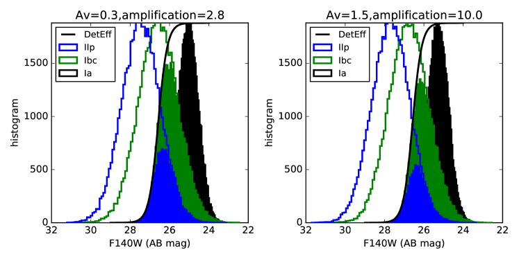
Figure 8: Monte Carlo simulation of supernova detectability by type, as the amount of dust is increased, and accounting for the See Change detection efficiency versus magnitude. The ratio of the area under the filled histograms to the open histograms is D${}_{\textrm{CC}}$ or D${}_{\textrm{Ia}}$ in Equation A1 (for D${}_{\textrm{CC}}$, the IIp and Ibc SNe are combined with equal weight). We find that for reasonable amplification values, the observable CC SN rate is highly impacted by the truncation of the detection efficiency curve, leading the observable SN rate in this galaxy to move towards SNe Ia at higher starburst fractions (see Figure 9).

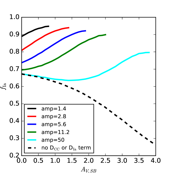
Figure 9: $f_{\mathrm{Ia}}$ using the modified rates from Equation A1, as a function of $A_{V,SB}$, for various amplification values with (solid) and without (dashed) the detection efficiency term. The $f_{\mathrm{Ia}}$ curves for different amplifications are shown only for D${}_{\textrm{CC}}>0.05$. For reasonable values of amplification, the CC SN magnitude distribution is truncated by the detection efficiency, and $R_{\mathrm{CC}}$ is dominated by the quickly declining D${}_{\textrm{CC}}$ term. For extremely high amplifications, the entire CC distribution is visible at low $A_{V,SB}$, so D${}_{\textrm{CC}}=1$; in this scenario, a small enhancement to $R_{\mathrm{CC}}$ occurs as the hidden starburst component increases, causing $f_{\mathrm{Ia}}$ to briefly decline with $A_{V,SB}$ until D${}_{\textrm{CC}}$ declines. We conclude that our primary typing algorithm, Equation 1, using $f_{\mathrm{Ia}}$ as in Equation 6.2, is conservative for the SN Ia probability, since the observable $R_{\mathrm{CC}}$ is in reality lower due to our magnitude limits.

Appendix B Is the redshift $2.22$ galaxy the SN host?

For use in Section 6, we now estimate the probability that this SN is merely projected on the $z=2.22$ galaxy, rather than hosted by it. As in Section 6, we consider the average likelihoods and rates for each type of SNe; for projected SNe, we must also consider these quantities over a range in redshift. We thus need three new ingredients 1) The likelihood as a function of redshift for CC SNe and SNe Ia. 2) The relative rates (per unit area, at the SN location) in the field and in the host. 3) The fraction of stellar mass and star-formation (and thus rate) that is excluded for this SN, as we do not see a second galaxy on top of the presumptive host.

For the likelihood as a function of redshift, we run the photometric typing at a range of redshifts and compute the equivalent redshift width for each type. This is defined relative to the likelihood at $z=2.22$, in the sense that averaging the likelihood over all redshifts gives the same answer as multiplying the $z=2.22$ value by the equivalent redshift width. We find this quantity is 0.35 for normal SNe Ia, 0.23 for SN 1991T-like SNe Ia, 1.93 for SNe Ib/c, and 0.93 for SNe II. The CC SN values are larger than for SNe Ia. The CC SNe have more heterogeneity, so they are consistent with the light curve over a wider range in redshift (i.e., a SN-only photo-z is not as accurate for a CC SN). As a special case, to test whether this SN could be an intra-cluster SN within MOO J1014+0038 having a chance alignment with a background galaxy, we also run the typing at the cluster redshift of 1.23. The best-fit likelihood values are $>100$ times lower, strongly disfavoring this possibility.

Now we need to consider the relative rates compared to the $z=2.22$ galaxy. From Rodney et al. (2014), the volumetric SN Ia rate in this redshift range is around $0.5\times 10^{-4}$ yr^-1 Mpc^-3 $h^{3}_{70}$. From Strolger et al. (2015), the volumetric CC SN rate in this redshift range is around $3.5\times 10^{-4}$ yr^-1 Mpc^-3 $h^{3}_{70}$. We must now transform these rates (and the above rates in the host galaxy) to observer-frame-rate surface densities evaluated at the SN location. For convenience, we work in per square arcsec units (although this is an arbitrary choice). From the factors in Equation 6.2, we estimate the global rates in the galaxy (0.0065 for SNe Ia and 0.0028 for CC SNe, both per rest-frame year); assuming the SN rates in the galaxy are roughly proportional to the rest-frame $B$-band ($F140W$) surface brightness (Heringer et al., 2017), we can find the rate surface density. Using a small aperture at the location of the SN (on an $F140W$ stacked image with no SN light), we measure the surface brightness. Multiplying this surface brightness by an area of one square arcsecond corresponds to 10% the luminosity of the $z=2.22$ galaxy. Thus, the SN rate per square arcsec is about 10% of the global galaxy rate, or 0.00028 for CC SNe and 0.00065 for SNe Ia (both per rest-frame year). For the volumetric rates, we would naively find 0.00032 CC SNe and 4.6$\times 10^{-5}$ SNe Ia per square arcsec, per unit redshift, per rest-frame year, but we must lower these by the amplification (as the volume behind the cluster is lowered by the same factor). To be conservative, we use the (smaller) weak-lensing amplification estimate of 1.75, for rates of 0.00019 (CC SNe) and 2.6$\times 10^{-5}$ (SNe Ia).

In some sense, the above volumetric rates count all expected galaxies along the line of sight, and thus double count the $z=2.22$ galaxy. They also count galaxies that would be clearly visible superposed on the $z=2.22$ galaxy (the vast majority of SN hosts). Thus, we must scale the rates by the fraction of star formation and stellar mass in galaxies too faint to detect in projection. Using only SN-free $F140W$ images, we measure a 95% upper limit for a point-like galaxy at the SN location of 0.2 e^-/s (after subtracting a smooth galaxy model for the $z=2.22$ galaxy). This is 28.2 (AB) as observed, or $\gtrsim 28.8$ after de-lensing. Assuming a redshift $\sim 2.22$, this corresponds to an absolute magnitude fainter than $16.2$ in rest-frame $B$ band. Comparing to the rest-frame $B$-band luminosity function at this redshift (Marchesini et al., 2007), we see that our limit is almost six magnitudes fainter than $M^{*}$. For a faint-end power law slope of $-1.5$, this would imply that 93% of $B$-band luminosity is excluded based on our upper limit. We apply this same factor to the SN rates; as we show, the probability of projection is small enough that reasonable variation in these assumptions does not affect the conclusion.

Finally, we complete the estimation of the projection probability, shown in Table 6. We collect the relative likelihood values from Section 6 and put them in the third column. The rates (per unit area and time for the $z=2.22$ galaxy, and per unit area, time, and $\Delta z$ for projections) are summarized in the fourth column. These are the only two quantities needed in the case that the $z=2.22$ galaxy is the host. However, we multiply by the redshift equivalent width for the projections, giving more probability to types of SNe which are consistent with the light curve over a longer redshift baseline. In the fifth column, we take the product of these factors, giving the rate-normalized likelihood for each type of SNe. In the final column, we show these values after normalizing to one. Summing the probabilities in the last four rows, we find the probability of a projection is $\sim 2\times 10^{-3}$.

Table 6: Extended typing analysis. The final column gives the probability of each scenario.

Host	SN Type	Relative Likelihood	Rate (Square Arcsec)-1 yr-1	Equivalent Redshift Width	Product	Normalized
			($\Delta z^{-1}$ for projections)
$z=2.22$	Ia	1	0.00063	$\cdots$	0.00063	0.898
$z=2.22$	Ia 1991T	2.67	2$\times 10^{-5}$	$\cdots$	5.2$\times 10^{-5}$	0.074
$z=2.22$	Ib/c	0.05	7$\times 10^{-5}$	$\cdots$	3.7$\times 10^{-6}$	0.005
$z=2.22$	II	0.07	0.00021	$\cdots$	1.4$\times 10^{-5}$	0.020
Projection	Ia	1	8.9$\times 10^{-6}$ $\times$ 0.07	0.35	6.2$\times 10^{-7}$	0.001
Projection	Ia 1991T	2.67	1.8$\times 10^{-7}$ $\times$ 0.07	0.23	3.4$\times 10^{-8}$	0.000
Projection	Ib/c	0.05	8.9$\times 10^{-5}$ $\times$ 0.07	1.93	3.3$\times 10^{-7}$	0.000
Projection	II	0.07	0.00013 $\times$ 0.07	0.93	6$\times 10^{-7}$	0.001

References

- Amanullah et al. (2010) Amanullah, R., Lidman, C., Rubin, D., et al. 2010, ApJ, 716, 712
- Amanullah et al. (2011) Amanullah, R., Goobar, A., Clément, B., et al. 2011, ApJ, 742, L7
- Balland et al. (2009) Balland, C., Baumont, S., Basa, S., et al. 2009, A&A, 507, 85
- Barro et al. (2017) Barro, G., Faber, S. M., Koo, D. C., et al. 2017, ApJ, 840, 47
- Belfiore et al. (2016) Belfiore, F., Maiolino, R., Maraston, C., et al. 2016, MNRAS, 461, 3111
- Bell & de Jong (2001) Bell, E. F., & de Jong, R. S. 2001, ApJ, 550, 212
- Betoule et al. (2014) Betoule, M., Kessler, R., Guy, J., et al. 2014, A&A, 568, A22
- Bohlin (2007) Bohlin, R. C. 2007, in Astronomical Society of the Pacific Conference Series, Vol. 364, The Future of Photometric, Spectrophotometric and Polarimetric Standardization, ed. C. Sterken, 315
- Bohlin et al. (2014) Bohlin, R. C., Gordon, K. D., & Tremblay, P.-E. 2014, PASP, 126, 711
- Brammer et al. (2011) Brammer, G. B., Whitaker, K. E., van Dokkum, P. G., et al. 2011, ApJ, 739, 24
- Brodwin et al. (2015) Brodwin, M., Greer, C. H., Leitch, E. M., et al. 2015, ApJ, 806, 26
- Bruzual & Charlot (2003) Bruzual, G., & Charlot, S. 2003, MNRAS, 344, 1000
- Calzetti et al. (2010) Calzetti, D., Wu, S.-Y., Hong, S., et al. 2010, ApJ, 714, 1256
- Cappellari (2017) Cappellari, M. 2017, MNRAS, 466, 798
- Cappellari & Emsellem (2004) Cappellari, M., & Emsellem, E. 2004, PASP, 116, 138
- Chabrier (2003) Chabrier, G. 2003, PASP, 115, 763
- Charlot & Fall (2000) Charlot, S., & Fall, S. M. 2000, ApJ, 539, 718
- Childress et al. (2014) Childress, M. J., Wolf, C., & Zahid, H. J. 2014, MNRAS, 445, 1898
- Clough et al. (1992) Clough, S. A., Iacono, M. J., & Moncet, J.-L. 1992, Journal of Geophysical Research: Atmospheres, 97, 15761
- Clough et al. (2005) Clough, S. A., Shephard, M. W., Mlawer, E. J., et al. 2005, J. Quant. Spec. Radiat. Transf., 91, 233
- Conley et al. (2006) Conley, A., Goldhaber, G., Wang, L., et al. 2006, ApJ, 644, 1
- Conroy et al. (2009) Conroy, C., Gunn, J. E., & White, M. 2009, ApJ, 699, 486
- Davidzon et al. (2017) Davidzon, I., Ilbert, O., Laigle, C., et al. 2017, A&A, 605, A70
- Decker et al. (in prep.) Decker, B., et al. in prep.
- Domínguez Sánchez et al. (2011) Domínguez Sánchez, H., Pozzi, F., Gruppioni, C., et al. 2011, MNRAS, 417, 900
- Duffy et al. (2008) Duffy, A. R., Schaye, J., Kay, S. T., & Dalla Vecchia, C. 2008, MNRAS, 390, L64
- Feulner et al. (2005) Feulner, G., Gabasch, A., Salvato, M., et al. 2005, ApJ, 633, L9
- Freudling et al. (2013) Freudling, W., Romaniello, M., Bramich, D. M., et al. 2013, A&A, 559, A96
- Gettings et al. (2012) Gettings, D. P., Gonzalez, A. H., Stanford, S. A., et al. 2012, ApJ, 759, L23
- Gilliland et al. (1999) Gilliland, R. L., Nugent, P. E., & Phillips, M. M. 1999, ApJ, 521, 30
- Gonzalez et al. (2015) Gonzalez, A. H., Decker, B., Brodwin, M., et al. 2015, ApJ, 812, L40
- Gonzalez et al. (in prep.) Gonzalez, A. H., et al. in prep.
- Goobar et al. (2009) Goobar, A., Paech, K., Stanishev, V., et al. 2009, A&A, 507, 71
- Goobar et al. (2017) Goobar, A., Amanullah, R., Kulkarni, S. R., et al. 2017, Science, 356, 291
- Gullikson et al. (2014) Gullikson, K., Dodson-Robinson, S., & Kraus, A. 2014, AJ, 148, 53
- Guy et al. (2007) Guy, J., Astier, P., Baumont, S., et al. 2007, A&A, 466, 11
- Hayden et al. (in prep.) Hayden, B., et al. in prep.
- Hayden et al. (2010) Hayden, B. T., Garnavich, P. M., Kessler, R., et al. 2010, ApJ, 712, 350
- Heringer et al. (2017) Heringer, E., Pritchet, C., Kezwer, J., et al. 2017, ApJ, 834, 15
- Hsiao et al. (2007) Hsiao, E. Y., Conley, A., Howell, D. A., et al. 2007, ApJ, 663, 1187
- Jimenez & Loeb (2002) Jimenez, R., & Loeb, A. 2002, ApJ, 573, 37
- Jones et al. (2013) Jones, D. O., Rodney, S. A., Riess, A. G., et al. 2013, ApJ, 768, 166
- Kelly et al. (2010) Kelly, P. L., Hicken, M., Burke, D. L., Mandel, K. S., & Kirshner, R. P. 2010, ApJ, 715, 743
- Kelly et al. (2015) Kelly, P. L., Rodney, S. A., Treu, T., et al. 2015, Science, 347, 1123
- Kelly et al. (2016a) —. 2016a, ApJ, 819, L8
- Kelly et al. (2016b) Kelly, P. L., Brammer, G., Selsing, J., et al. 2016b, ApJ, 831, 205
- Kessler et al. (2009) Kessler, R., Bernstein, J. P., Cinabro, D., et al. 2009, PASP, 121, 1028
- Kessler et al. (2010) Kessler, R., Bassett, B., Belov, P., et al. 2010, PASP, 122, 1415
- Kim et al. (in prep.) Kim, S., et al. in prep.
- Kissler-Patig et al. (2008) Kissler-Patig, M., Pirard, J.-F., Casali, M., et al. 2008, A&A, 491, 941
- Kriek & Conroy (2013) Kriek, M., & Conroy, C. 2013, ApJ, 775, L16
- Kriek et al. (2009) Kriek, M., van Dokkum, P. G., Labbé, I., et al. 2009, ApJ, 700, 221
- Kron (1980) Kron, R. G. 1980, ApJS, 43, 305
- Levan et al. (2005) Levan, A., Nugent, P., Fruchter, A., et al. 2005, ApJ, 624, 880
- Li et al. (2011) Li, W., Leaman, J., Chornock, R., et al. 2011, MNRAS, 412, 1441
- Lochner et al. (2016) Lochner, M., McEwen, J. D., Peiris, H. V., Lahav, O., & Winter, M. K. 2016, ArXiv e-prints, arXiv:1603.00882
- Maccoun & Perlmutter (2015) Maccoun, R., & Perlmutter, S. 2015, Nature, 526, 187
- Madau & Dickinson (2014) Madau, P., & Dickinson, M. 2014, ARA&A, 52, 415
- Mandel et al. (2016) Mandel, K. S., Scolnic, D., Shariff, H., Foley, R. J., & Kirshner, R. P. 2016, ArXiv e-prints, arXiv:1609.04470
- Mannucci et al. (2006) Mannucci, F., Della Valle, M., & Panagia, N. 2006, MNRAS, 370, 773
- Maoz & Mannucci (2012) Maoz, D., & Mannucci, F. 2012, PASA, 29, 447
- Marchesini et al. (2007) Marchesini, D., van Dokkum, P., Quadri, R., et al. 2007, ApJ, 656, 42
- Meyers et al. (2012) Meyers, J., Aldering, G., Barbary, K., et al. 2012, ApJ, 750, 1
- Moresco et al. (2012) Moresco, M., Cimatti, A., Jimenez, R., et al. 2012, J. Cosmology Astropart. Phys, 8, 006
- Mosher et al. (2014) Mosher, J., Guy, J., Kessler, R., et al. 2014, ApJ, 793, 16
- Muzzin et al. (2012) Muzzin, A., Labbé, I., Franx, M., et al. 2012, ApJ, 761, 142
- Navarro et al. (1997) Navarro, J. F., Frenk, C. S., & White, S. D. M. 1997, ApJ, 490, 493
- Newman et al. (2015) Newman, A. B., Belli, S., & Ellis, R. S. 2015, ApJ, 813, L7
- Nordin et al. (2014) Nordin, J., Rubin, D., Richard, J., et al. 2014, MNRAS, 440, 2742
- Nugent et al. (2002) Nugent, P., Kim, A., & Perlmutter, S. 2002, PASP, 114, 803
- Pandya et al. (2017) Pandya, V., Brennan, R., Somerville, R. S., et al. 2017, MNRAS, 472, 2054
- Patel et al. (2014) Patel, B., McCully, C., Jha, S. W., et al. 2014, ApJ, 786, 9
- Petrushevska et al. (2016) Petrushevska, T., Amanullah, R., Goobar, A., et al. 2016, A&A, 594, A54
- Planck Collaboration et al. (2015) Planck Collaboration, Ade, P. A. R., Aghanim, N., et al. 2015, ArXiv e-prints, arXiv:1502.01589
- Quimby et al. (2014) Quimby, R. M., Oguri, M., More, A., et al. 2014, Science, 344, 396
- Rafelski et al. (2015) Rafelski, M., Teplitz, H. I., Gardner, J. P., et al. 2015, AJ, 150, 31
- Richardson et al. (2014) Richardson, D., Jenkins, III, R. L., Wright, J., & Maddox, L. 2014, AJ, 147, 118
- Rigault et al. (2013) Rigault, M., Copin, Y., Aldering, G., et al. 2013, A&A, 560, A66
- Rodney & Tonry (2009) Rodney, S. A., & Tonry, J. L. 2009, ApJ, 707, 1064
- Rodney et al. (2012) Rodney, S. A., Riess, A. G., Dahlen, T., et al. 2012, ApJ, 746, 5
- Rodney et al. (2014) Rodney, S. A., Riess, A. G., Strolger, L.-G., et al. 2014, AJ, 148, 13
- Rodney et al. (2015a) Rodney, S. A., Patel, B., Scolnic, D., et al. 2015a, ApJ, 811, 70
- Rodney et al. (2015b) Rodney, S. A., Riess, A. G., Scolnic, D. M., et al. 2015b, AJ, 150, 156
- Rubin et al. (2013) Rubin, D., Knop, R. A., Rykoff, E., et al. 2013, ApJ, 763, 35
- Rubin et al. (2015) Rubin, D., Aldering, G., Barbary, K., et al. 2015, ApJ, 813, 137
- Rubin et al. (in prep.) Rubin, D., et al. in prep.
- Sako et al. (2011) Sako, M., Bassett, B., Connolly, B., et al. 2011, ApJ, 738, 162
- Salpeter (1955) Salpeter, E. E. 1955, ApJ, 121, 161
- Scalzo et al. (2012) Scalzo, R., Aldering, G., Antilogus, P., et al. 2012, ApJ, 757, 12
- Scannapieco & Bildsten (2005) Scannapieco, E., & Bildsten, L. 2005, ApJ, 629, L85
- Schlafly et al. (2016) Schlafly, E. F., Meisner, A. M., Stutz, A. M., et al. 2016, ApJ, 821, 78
- Scolnic & Kessler (2016) Scolnic, D., & Kessler, R. 2016, ApJ, 822, L35
- Scolnic et al. (2014) Scolnic, D. M., Riess, A. G., Foley, R. J., et al. 2014, ApJ, 780, 37
- Sérsic (1963) Sérsic, J. L. 1963, Boletin de la Asociacion Argentina de Astronomia La Plata Argentina, 6, 41
- Silverman et al. (2012) Silverman, J. M., Kong, J. J., & Filippenko, A. V. 2012, MNRAS, 425, 1819
- Skrutskie et al. (2006) Skrutskie, M. F., Cutri, R. M., Stiening, R., et al. 2006, AJ, 131, 1163
- Stanford et al. (2014) Stanford, S. A., Gonzalez, A. H., Brodwin, M., et al. 2014, ApJS, 213, 25
- Stanishev et al. (2009) Stanishev, V., Goobar, A., Paech, K., et al. 2009, A&A, 507, 61
- Stern et al. (2010) Stern, D., Jimenez, R., Verde, L., Kamionkowski, M., & Stanford, S. A. 2010, J. Cosmology Astropart. Phys, 2, 008
- Stern et al. (2004) Stern, D., van Dokkum, P. G., Nugent, P., et al. 2004, ApJ, 612, 690
- Strolger et al. (2015) Strolger, L.-G., Dahlen, T., Rodney, S. A., et al. 2015, ApJ, 813, 93
- Sullivan et al. (2006) Sullivan, M., Le Borgne, D., Pritchet, C. J., et al. 2006, ApJ, 648, 868
- Sullivan et al. (2010) Sullivan, M., Conley, A., Howell, D. A., et al. 2010, MNRAS, 406, 782
- Suzuki et al. (2012) Suzuki, N., Rubin, D., Lidman, C., et al. 2012, ApJ, 746, 85
- Tody (1993) Tody, D. 1993, in Astronomical Society of the Pacific Conference Series, Vol. 52, Astronomical Data Analysis Software and Systems II, ed. R. J. Hanisch, R. J. V. Brissenden, & J. Barnes, 173
- Tripp (1998) Tripp, R. 1998, A&A, 331, 815
- van der Wel et al. (2014) van der Wel, A., Franx, M., van Dokkum, P. G., et al. 2014, ApJ, 788, 28
- van Dokkum et al. (2015) van Dokkum, P. G., Nelson, E. J., Franx, M., et al. 2015, ApJ, 813, 23
- Vernet et al. (2011) Vernet, J., Dekker, H., D’Odorico, S., et al. 2011, A&A, 536, A105
- Whitaker et al. (2013) Whitaker, K. E., van Dokkum, P. G., Brammer, G., et al. 2013, ApJ, 770, L39
- Williams et al. (2009) Williams, R. J., Quadri, R. F., Franx, M., van Dokkum, P., & Labbé, I. 2009, ApJ, 691, 1879
- Wright et al. (2010) Wright, E. L., Eisenhardt, P. R. M., Mainzer, A. K., et al. 2010, AJ, 140, 1868