Multifractal study of quasiparticle localization in disordered superconductors

Abstract

The thermal metal to thermal insulator transition due to random disorder is studied in the context of the symmetries of the Bogoliubov de Gennes Hamiltonian. We focus on a three dimensional system with gapless s-wave pairing that possesses time reversal and spin rotational symmetry. The quasiparticle excitations (bogolons) undergo a metal insulator transition as the disorder increases. We determine the critical disorder strength and correlation exponent first by the transfer matrix method (TMM). We then apply a multifractal finite sized scaling (MFSS) of the bogolon wavefunction obtained from large scale diagonalization of the Hamiltonian and obtain the critical disorder strength and exponent, in agreement with those found by TMM.

I Introduction

Anderson localization involves the localization of single-particle electronic states in a disordered metalAnderson1958 . Although this has proved to be a challenging and complex problemKMreview , the basic interpretation of the transition is clear: it is a transition from a metallic phase where electrons are able to diffuse and transport over long distances to an insulating phase where this is prevented. Anderson localization occurs in normal electronic systems (most famously dopedPaalanenThomas1983 and amorphousMottDavis1979 semiconductors). The conducting electronic states are separated from the insulating states by a mobility edge in energy and disorder strength. Many features of the localization transition have been studied and much attention has been paid to two in particular: the multifractality of critical wave functions at the transition and the role played by the symmetries of the Hamiltonian Atland1997 ; Schnyder2008 ; Wigner1955 ; Castellani1986 .

The Anderson transition was first and most studied for Hamiltonians of the three Wigner-DysonWigner1955 symmetry classes. The identification of additional symmetry classes (bringing the full number to tenAtland1997 ) has lead to the study of the effects of Anderson localization beyond the original three symmetry classes and the additional rich phenomenaFerdinand2008 . In this paper, we consider the question of quasiparticle localization in the Bogoliubov de Gennes class for three dimensions with time reversal and spin rotation symmetry (class CI) which we use to model a dirty superconductor with a finite density of states at the Fermi level. The excitations of this class are Bogoliubov quasiparticlesBogoliubov1958 (also referred to as bogolons in this paper) with no definite charge as they are a superposition of electron and hole excitations Beenakker2015 , so this is different from the case of the Anderson model where the excitations have a well defined charge. In this case, the localization transition is interpreted as localization of bogolons that occurs within the superconducting phase. The two phases are refereed to as a “thermal metal” where the bogolons are extended and a “thermal insulator” where they are localizedvish1999 . As mentioned above, the quasiparticles do not transport charge and so there is no Weidemann-Franz law between the thermal and electric transport, but there is still thermal transport and so on the localized side of the transition the system will be thermally insulating and on the extended side it will be thermally metallic vish1999 .

The idea of multifractality was introduced by MandlebrotMandelbrot1974 ; Halsey1986 and describes spatial structures that have a complicated distribution and require an infinite number of critical exponents to describe the scaling of their moments. The multifractal nature of the wavefunction at criticality was realized for Anderson transitions wegner1980 ; Castellani1986 and is now recognized as a defining characteristic. A proposed generalization of the multifractal analysis can be used to calculate the critical parameters of the Anderson transitionRodriguez2010 ; Rodriguez2011 ; Ujfalusi2015 which has even been applied to calculations of doped semiconductorsharashima2014 .

In this paper, we apply the generalized multifractal finite size scaling (MFSS) Rodriguez2010 ; Rodriguez2011 analysis to a simple model of a dirty superconductor. The model Hamiltonian and methods of extracting critical parameters which include transfer matrix method and multifractal analysis are described in Sec.II. We will demonstrate that the multifractal analysis can be used to extract the critical disorder strength by showing agreement with transfer matrix method calculations and confirms that this transition falls outside the Wigner-Dyson symmetry class. Also, we will argue that the multifractal character of the wavefunctions can possibly explain some experimental findings on dirty superconductors, such as the increase in $T_{c}$ with disorder. These results are presented in Sec.III and discussed in Sec.III.1. We conclude in Sec. IV

II Model and methods

II.1 Model of Dirty Superconductor

We study our model of a dirty superconductor within the mean field Bogoliubov-de Gennes approximation, and so the Hamiltonian is given by

$$H=\sum_{i,j}[t_{i,j}\sum_{\sigma=\uparrow,\downarrow}(c_{i,\sigma}^{\dagger}c_{j,\sigma}+H.c)+\Delta_{i,j}(c_{i,\uparrow}^{\dagger}c_{j,\downarrow}^{\dagger}+H.c.)].$$ (1)

The annihilation operator for site $i$ with spin $\sigma$ is given by $c_{i,\sigma}$, and similarly for the creation operators. We only consider spin one-half fermions in this study, so $\sigma=\uparrow$ or $\downarrow$. $t_{i,j}$ and $\Delta_{i,j}$ are the hopping and pairing between site $i$ and $j$ respectively.

Previous studies of dirty superconductors predominately focused on the pairing with conventional s-wave symmetry with on-site pairing which has a spectral gap at the band center. Without disorder, the spectral function is given by $E({\bf k})=\sqrt{\Delta({\bf k})^{2}+\epsilon({\bf k})^{2}}$, and for a cubic lattice $\epsilon({\bf k})=-2t\sum_{i=x,y,z}\cos(k_{i})$. For the case of conventional s-wave pairing, we have $\Delta({\bf k})=\Delta_{0}$ a constant. Since we do not expect for gap formation to be required for multifractal behavior of the wavefunction, we instead focus on a gapless superconductor. A simple choice is one with extended s-wave pairing with the same nodal structure as that of the bare dispersion $\epsilon({\bf k})$ vish2001 , in which $\Delta({\bf k})=\Delta_{0}\sum_{i=x,y,z}\cos(k_{i})$.

Random disorder is introduced via two independent terms, one for the on-site local potential and the other for the on-site pairing. Following the convention in Ref. vish2001, , the total Hamiltonian may be written as

$$H=H_{0}+H_{dis},$$ (2)

$$H_{0}=\sum_{<i,j>}[\frac{1}{\sqrt{2}}\sum_{\sigma=\uparrow,\downarrow}(c_{i,\sigma}^{\dagger}c_{j,\sigma}+H.c)+\frac{1}{\sqrt{2}}(c_{i,\uparrow}^{\dagger}c_{j,\downarrow}^{\dagger}+H.c.)],$$ (3)

$$H_{dis}=\sum_{i}[\epsilon_{i}\sum_{\sigma=\uparrow,\downarrow}(c_{i,\sigma}^{\dagger}c_{i,\sigma}+H.c)+\Delta_{i}(c_{i,\uparrow}^{\dagger}c_{i,\downarrow}^{\dagger}+H.c.)].$$ (4)

The disorder in onsite potential and onsite pairing is assumed to be uniformly distributed from $-W$ to $W$, and so $P(\epsilon_{i})=P(\Delta_{i})=1/2W~{}\forall~{}-W<\epsilon_{i},\Delta_{i}<W$. The Hamiltonian possesses time reversal symmetry, spin rotation symmetry and particle-hole symmetry which dictates that eigenstates always come in pairs with energy $E$ and $-E$. These symmetries put the Hamiltonian into the CI class Atland1997 .

II.2 Transfer Matrix Method

We first locate the critical point of the model and its localization length exponent using the transfer matrix method. The three dimensional system has a width and height equal to $M$ for each slice of a $N$-slice cuboid, forming a “bar” of length $N$. The Hamiltonian can be decomposed into the form

$$H=\sum_{i}H_{i}+\sum_{i}(H_{i,i+1}+H.c.),$$ (5)

where $H_{i}$ describes the Hamiltonian for slice $i$ and $H_{i,i+1}$ is the coupling terms between the $i$ and $i+1$ slices. The Schrödinger equation can be written in the form

$${H}_{n,n+1}c_{n+1}=(E-{H}_{n})c_{n}-{H}_{n,n-1}c_{n-1}$$ (6)

where $c_{i}$ is the $M^{2}$ components wavefunction of the slice $i$. We introduce the transfer matrix

$$T_{i}=\begin{bmatrix}H_{i,i+1}^{-1}(E-H_{i})&-H_{i,i+1}^{-1}H_{i-1,i}\\ 1&0\end{bmatrix}$$ (7)

and Eq.6 can be interpreted as the iteration of

$$\left[\begin{array}[]{c}c_{i+1}\\ c_{i}\end{array}\right]=T_{i}\times\left[\begin{array}[]{c}c_{i}\\ c_{i-1}\end{array}\right].$$ (8)

The goal of the transfer matrix method is to calculate the localization length, $\lambda_{M}(E)$, from the product of $N$ transfer matricies

$$\tau_{N}\equiv\prod_{i=1}^{N}T_{i}.$$ (9)

The Lyapunov exponents of the matrix $\tau_{N}$ is given by the logarithm of its eigenvalues. The smallest exponent corresponds to the slowest exponential decay of the wavefunction and thus can be identified as corresponding to the localization length, $\lambda_{M}(E)$. The localization length is computed by repeated multiplication of $T_{i}$, but since the multiplication of matrices is numerically unstable periodic reorthogonalization is needed in the numerical implementationKramer2010 . We use a QR decomposition for reorthogonalization implemented by LAPACKLAPACK , and so at the $s$ reorthogonalization step the matrix (corresponding to some intermediate $L$’th multiplication in calculating Eq.9) the matrix is decomposed

$$\tau_{L}=QR$$ (10)

where $R$ is an upper triangular matrix and the Lyapunov exponents $\gamma_{s}$ are calculated as

$$\gamma_{s}=\gamma_{s-1}+\log b_{s}$$ (11)

where $b_{s}$ are the $2M^{2}$ diagonal elements of $R$ for the $s$ renormalization step. The multiplication of transfer matrices is then continued with the $Q$ matrix. The slowest decaying exponent ($\gamma_{\ell}$) is used to compute the localization length $\lambda_{M}(E)=1/\gamma_{\ell}$ for a given width $M$ and energy $E$.

The localization length is then used to calculate the the Kramer-MackinnonMacKinnonKramer1983 scaling parameter $\Lambda_{M}(E)=\lambda_{M}(E)/M$ which is expected to scale as

$$\Lambda_{M}=\frac{\lambda_{M}}{M}=f\left(\frac{M}{\xi}\right),$$ (12)

where $\xi\propto|W-W_{c}|^{-\nu}$. The scaling function $f$ is Taylor expanded about the critical point $W_{c}$ and the critical parameters $W_{c}$ and $\nu$ enter as fitting parameters and so can be determined by a least-squares minimization.

II.3 Multifractal Analysis

We consider the multifractal properties of the bogolon wave-function $|\psi_{i}|^{2}=|u_{i}|^{2}+|v_{i}|^{2}$ for a three dimensional simple cubic lattice of linear size $L$. The method is based on the study of Anderson models in Wigner-Dyson class. Rodriguez2010 ; Rodriguez2011 ; Ujfalusi2015 This cubic wavefunction is partitioned into boxes of linear size $\ell$. We introduce the quantity $\lambda=\ell/L$ and so we have $N_{b}=\lambda^{-d}$ as the number of boxes where $d$ is the dimensionality of the system. In this paper, we shall only consider $d=3$. We introduce the “coarse grained” box measure

$$\mu_{b(\ell)}=\sum_{i\in b(\ell)}|\psi_{i}|^{2}$$ (13)

where $b(\ell)$ indexes the $N_{b}$ boxes for a given box size $\ell$. We introduce for convenienceRodriguez2011 the quantity

$$\alpha\equiv\frac{\log\mu}{\log\lambda}$$ (14)

to work with instead of directly with the box measures given in Eq.13. Multifractility implies that the number of boxes that correspond to a given $\alpha$ (we denote as $N(\alpha)$) must scale as

$$N(\alpha)\sim\lambda^{-f(\alpha)}$$ (15)

where $f(\alpha)$ is some fractal dimension that depends on $\alpha$. For the case where $|\psi|^{2}$ are distributed uniformly in space, one would expect there to be only a singular $\alpha$ and from the definition of $\lambda$ above $f(\alpha)=d$. However, for finite $\lambda$ a narrow distribution peaked around $f(\alpha)=d$ would be expected and so the above Eq.15 is only defined in the limit $\lambda\rightarrow 0$. The fact that there exists an $\alpha$ dependent spectrum $f(\alpha)$ characterizes a system as being multifractalNakayama2003 .

We will want to consider the $q$-dependent moments of the distribution of $\alpha$ or $\alpha(q)$. We first introduce the generalized inverse participation ratios for the coarse grained distributions $P(\mu_{b(\ell)})$ as

$$R_{q}=\sum_{b(\ell)}^{N_{b}}\left(\mu_{b(\ell)}\right)^{q}$$ (16)

and assume (similarly to Eq.15) that the moments of the distribution of each box measure scale by the $q$ dependent exponents $\tau(q)$ or

$$\langle R_{q}\rangle\sim\lambda^{\tau(q)}$$ (17)

where $\langle\cdot\cdot\cdot\rangle$ denotes an ensemble average. It can be shownNakayama2003 that $f(\alpha)$ and $\tau(q)$ can be related by a Legendre transform

$$f(\alpha)=-\tau(q)+q\alpha\,,$$ (18)

where

$$\alpha(q)=\frac{d\tau(q)}{dq}.$$ (19)

Carrying out the differentiation in Eq.19 and using the definition of $\tau(q)$ in Eq.17 leads to the expression

$$\alpha(q)=\lim_{\lambda\rightarrow 0}\frac{\langle S_{q}\rangle}{\log\lambda\langle R_{q}\rangle}$$ (20)

where

$$S_{q}=\sum_{k}^{N_{b}}\mu_{k}^{q}\log\mu_{k}.$$ (21)

As defined above, the multifractal exponents are only strictly defined in the limit of infinite system size ($\lambda\rightarrow 0$ as mentioned above) and at the critical point. However, they can be defined for fixed $\lambda$ which we denote with a tilde as

$$\tilde{\alpha}_{q}=\frac{\langle S_{q}\rangle}{\log\lambda\langle R_{q}\rangle}.$$ (22)

The error in $\tilde{\alpha}_{q}$, $\sigma_{\tilde{\alpha}}$, is then estimated from standard propagation of uncertainty

$$\left(\frac{\sigma_{\tilde{\alpha}}}{\tilde{\alpha}}\right)^{2}=\left(\frac{\sigma_{\langle S_{q}\rangle}}{\langle S_{q}\rangle}\right)^{2}+\left(\frac{\sigma_{\langle R_{q}\rangle}}{\langle R_{q}\rangle}\right)^{2}-2\left(\frac{\sigma_{\langle R_{q}\rangle\langle S_{q}\rangle}}{\langle R_{q}\rangle\langle S_{q}\rangle}\right)^{2}$$

where the covariance term $\sigma_{\langle S_{q}\rangle\langle R_{q}\rangle}$ is kept to account for correlations as $R_{q}$ and $S_{q}$ are computed from the same data set.

The quantity $\tilde{\alpha}_{q}$ scales according to standard one parameter scaling for fixed $\lambda$ in a relevant ($\rho$) and an irrelevant ($\eta$) scaling variable or Rodriguez2010 ; Rodriguez2011

$$\tilde{\alpha}_{q}(W,L)=G(\rho L^{1/\nu},\eta L^{-|y|}).$$ (23)

We expand the scaling function to first order in the irrelevant operator $\eta$

$$\tilde{\alpha}_{q}(W,L)=G^{(0)}(\rho L^{1/\nu})+\eta L^{-|y|}G^{(1)}(\rho L^{1/\nu}),$$ (24)

where the sub-leading term is characterized by $\eta,y$, and $G^{(1)}$. The function $G^{(s)}$ (where $s=0,1$ from above) is expanded as a Taylor series

$$G^{(s)}(L^{1/\nu})=\sum_{k=0}^{n_{s}}a_{sk}\rho^{k}L^{k/\nu}.$$ (25)

The scaling fields $\rho$ and $\eta$ are likewise expanded in terms of $w=(W-W_{c})/W_{c}$ as

$$\rho(w)=w+\sum_{m=2}^{m_{\rho}}b_{m}w^{m}$$ (26)

and

$$\eta(w)=1+\sum_{m=1}^{m_{\eta}}c_{m}w^{m}.$$ (27)

The critical parameters ($W_{c}$, $\nu$) and the irrelevant scaling exponent $y$ are determined by fitting the data for $\tilde{\alpha}_{q}(W,L)$ to Eq.24. In addition, we have $n_{0}+n_{1}+m_{\rho}+m_{\eta}$ Taylor expansion parameters. The correlation length is $\xi=|\rho(\omega)|^{-\nu}$ and so the scaled $\tilde{\alpha}_{q}(W,L)$ data (which we denote as $\tilde{\alpha}^{\rm corr}_{q})$ collapses onto two branches

$$\tilde{\alpha}^{\rm corr}_{q}=G_{q}^{(0)}(\pm(L/\xi)^{1/\nu})$$ (28)

III Results

We employ the transfer matrix method to find the critical disorder strength by performing a finite size scaling analysis as shown in Fig.1. We will compare this result with that predicted by multifractal analysis of the bogolon wavefunction. The fitting is performed using the SciPy package which acts as a wrapper to MINPACK to perform the least squares minimization scipy_ref ; minpack_ref . The fitting range used in Fig.1 is determined by performing multiple fits and choosing the one that approximately provides the minimum for the sum of squares. This range is then used for $100$ bootstrapped resamples of the data to estimate the error bars. Note however that there can still be error in choosing the fitting range so the error bars are most likely under-estimated. The calculation was performed for $E=0$ as were are interested in only the lowest energy excitations which will also be the focus in the following multifractal analysis.

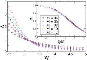
Figure 1: Kramer-Mackinnon scaling parameter as a function of disorder strength calculated with the transfer matrix method for a bar of length $N=20000$, $E=0$ and a QR reorthogonalization is performed after every $5$ multiplications. Note the crossing indicating a critical disorder strength around $W=3.2$. When the finite size scaling is performed as described in II.2 the data collapses as is shown in the inset. A bootstrap re-sampling is performed to generate $100$ data sets to estimate the fitting parameters yielding $W_{c}=3.212\pm 0.008$ and a critical exponent of $\nu=1.01\pm 0.05$.

For the multifractal analysis of the bogolon wavefunctions, we use the JADAMALU package which implements a Jacobi-Davidson method with preconditioningJADAMALU ; JADAMALU_code to diagonalize the Hamiltonian. In contrast to that of the conventional Anderson model, the disorder terms for the present model appear in the off-diagonal elements. This poses as a challenge for attaining convergence by the iterative algorithm, both in term of the memory storage and floating point operation. Therefore the accessible system sizes are limited in comparison to that of the models with diagonal disorder terms. Rodriguez2010 ; Rodriguez2011 Table 1 lists the number of realizations generated for different system size and disorder strength. We keep only one state from each realization with the closest eigenvalue (and associated eigenvector) to zero. This is to prevent correlations in wavefunctions that come from the same realization of disorder. The wave function can then be coarse grained (as described in Sec.II.3) and the distribution of $\alpha$ is plotted in in Fig.2.

We can then calculate $\tilde{\alpha}_{q}$ for $q=0$ (given by Eq.22 which we denote as $\tilde{\alpha}_{0}$) and is plotted in Fig.3 as a function of system size and disorder strength which is expected to show the characteristic finite size behavior and exhibit a crossing at the critical disorder strengthRodriguez2011 Rodriguez2010 . We also carry out multifractal finite size scaling for fixed $\lambda$ and we assume our data $y_{i}$ (with uncertainty $\sigma_{i}$) is uncorrelated (as we only consider fixed $\lambda$ so each point is from it’s own realization) and thus the $\chi^{2}$ statistic for our model fits $f_{i}$ is

$$\chi^{2}=\sum_{i}\frac{(y_{i}-f_{i})^{2}}{\sigma_{i}^{2}}$$ (29)

The order of expansion in $n_{0}$, $n_{1}$, $m_{\eta}$ and $m_{\rho}$ is determined by choosing the fit that keeps the $\chi^{2}$ statistic small, keeps the order of expansion small and provides a “good” collapse of the data into two branches. Error bars in fitting parameters are determined by generating new values of $\langle S_{q}\rangle$ and $\langle R_{q}\rangle$ for each corresponding $L$ and $W$ by pulling from a Gaussian distribution with mean $\langle S_{q}\rangle$ and variance $\sigma_{\langle S_{q}\rangle}/\sqrt{N-1}$ where N is the number of samples of $S_{q}$ and this is likewise done for $\langle R_{q}\rangle$. This allows for a new calculation of $\alpha_{q}$. The result from this procedure yields $Wc=3.208\pm 0.007$ and $\nu=0.97\pm 0.06$ in agreement with the above transfer matrix study. All simulation parameters used for the calculation of the bogolon wave functions is collected in Sec.V

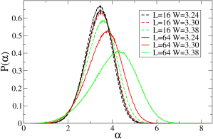
Figure 2: Distribution of the quantity $\alpha$ (defined in Eq.14) for a finite value of $\lambda=1/8$ for various system sizes and two disorder strengths. The behavior of the distributions as a function of $L$ motivates the application of the multifractal analysis in the Ref. Rodriguez2011, as when the transition is approached ($\sim 3.2$) the distributions become more scale invariant (not depending on system size).

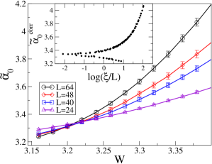
Figure 3: The multifractal exponent $\alpha_{0}$ as a function of disorder strength $W$ that exhibits scaling behavior around the critical disorder strength $W=3.2$. The inset shows the data collapse into after performing the finite size scaling and plotting the scaling function for both branches of $\tilde{\alpha_{0}}$ in Eq. 28. The critical parameters used are $W_{c}=3.21$, $\nu=1.09$, $y=15.94$. The orders of expansion used for $G^{(0)},G^{(1)},\rho$, and $\eta$ are $n_{0}=2,n_{1}=2,m_{\rho}=1$ and $m_{\eta}=0$ respectively. The resulting $\chi^{2}=22$. The fit was chosen by keeping the order of expansion low and taking the smallest $\chi^{2}$ for which the data collapse close to the fitting function $\tilde{\alpha_{0}}$.

III.1 Discussion

It has been established by the work of Ref. [vish2001, ] that the exponent $\nu$ is much different than the Anderson model. We confirm this with our multifractal analysis, establishing that this falls outside the Wigner-Dyson (WD) symmetry class.

The motivation for studying models of disordered superconductors is the rich variety of unusual properties they can exibit such as an enhanced single particle energy gap that persists even after superconductivity is destroyed Feigelman2007 . Specific to this paper, the motivation for studying the multifractal character of the eigenstates is the proposal that multifractility can lead to enhancements of the critical temperature at which superconductivity is destroyed ($T_{c}$)Burmistrov2012 ; Mayoh2015 which is observed in thin superconducting films that are weakly disordered, namely Aladams2 Abeles1966 wich is still not well understood. An explanation for the enhancement of $T_{c}$ due to multifractility is that multifractility implies a broad distribution of exponents for the spatial correlations at the transition (given by $f(\alpha)$). This can be understood by the fact that there are regions of the system that have exponents that will decay off more slowly than if there were only a single one, implying stronger correlations among bogolon wavefunction $|\psi_{i}|^{2}$. It is known that the regions of large $|\psi_{i}|^{2}$ for the lowest excitations will correspond to regions of large local pairing amplitude $\Delta_{i}$nandiniBook nandini2001 , and so $\Delta_{i}$ will also realize multifractal correlations. The result of the longer range correlations would lead to stronger pairing correlations, resulting in an increase in $T_{c}$. Given the present calculations are done with a fixed distribution of $\Delta_{i}$, we cannot address quantitatively the relation between the $T_{c}$ and the disorder.

Furthermore, it is known that the presence of bogolon excitations is what dissipates momentum and disrupts the flow of super current, destroying superconductivityLancaster2014 . Therefore, a state in which the excitations are localized would help to “protect” superconductivity at finite temperatures and increase $T_{c}$. As the localization effect would be very strong in a quasi-2D system, when a superconducting film is made more thin the bogolons must become localized. The reason it is not observed for all thin films (it is more typical for $T_{c}$ to decrease) is that if the disorder is strong this effect will not be observed because strong disorder is already destroying the superconductivity as it destroys the long range phase coherenceLiu1993 .

Finally, we note that the multifractal analysis used here could be applied to models of conventional s-wave superconductivity with disorder which has been well studied Ghosal2001 ; Kamar2014 ; Jiang2013 ; Sakaida2013 ; Seibold2012 ; Sacepe2011 ; Bouadim2011 ; Aryanpour2007 . This is important because the transfer matrix method cannot be used to locate the localization transition if the pairing must be solved self-consistently as this creates a correlation between layers Qin2005 . However, as all that is needed is the wavefunction for this method, the multifractal finite size scaling analysis could be applied.

IV Conclusion

We conclude that the multifractal analysis that works for the Anderson model can also be used for models of disordered superconductors to find the localization transition of the quasi particle excitations. In addition, it also confirms that the thermal metal to thermal insulator is indeed in a separate universality class from the Anderson model. vish2001

Future work would include addressing the question of the relation between multifractility of critical wavefunctions and the impact on $T_{c}$ more directly by finding the transition temperature for a model of a conventional s-wave superconductor by solving the pairing field $\Delta_{i}$ self consistently for a given attraction interaction strength $U$. nandini2001 The multifractal spectrum $f(\alpha)$ could then be compared as a function of interaction strength and $T_{c}$ to quantitatively address the role played by multifractal eigenstates and coupling strength on the critical temperature. Also, the question of whether this method can detect the superconductor to insulator transition Ghosal2001 would be of interest as this model could not be studied with transfer matrix due to the self consistency requirement on the pairing.

V Appendix A: Multifractal System Parameters

In the TABLE 1, are the number of realizations (in the units of 1000 realizations) used for the calculation of the bogolon wavefunctions where $L$ is the linear system size, $W$ the disorder strength and $N_{R}$ the number of realizations. In TABLE 2, we test effects of the order of expansion of the fitting functions. The table lists the $\chi^{2}$ obtained as a function of $n_{0}$, $n_{1}$, $m_{\rho}$, and $m_{\eta}$. See Eq. 25, 26, and 27 for their definitions.

	$24$	$32$	$40$	$48$	$56$	$64$
3.16	20	20	14	3.2	3.2	3.2
3.18	20	20	14	3.2	3.2	3.2
3.20	20	20	14	3.2	3.2	3.2
3.22	20	20	14	3.2	3.2	3.2
3.24	80	40	30	10	8	4
3.26	80	40	30	10	8	4
3.28	80	40	30	10	8	4
3.30	80	40	30	10	8	4
3.32	80	40	30	10	8	4
3.34	80	40	30	10	8	4
3.36	80	40	30	10	8	4
3.38	80	40	30	10	8	4
3.40	80	40	30	10	0	0

Table 1: Number of realizations as a function of $W$ and $L$. The number of realizations is in the units of 1000 realizations.

$n_{0}$	$n_{1}$	$m_{\rho}$	$m_{\eta}$	$\chi^{2}$
2	0	1	0	15.55
2	1	1	0	15.55
3	0	1	0	15.20
3	1	1	0	15.20
2	0	1	1	15.55
2	1	1	1	15.55
3	0	1	1	15.20
3	1	1	1	15.20
2	0	2	0	15.54
2	1	2	0	15.54
3	0	2	0	14.67
3	1	2	0	14.67
2	0	2	1	15.54
2	1	2	1	15.54
3	0	2	1	14.67
3	1	2	1	14.67
2	0	2	2	15.54
2	1	2	2	15.54
3	0	2	2	14.67
3	1	2	2	14.67
2	0	3	0	15.21
2	1	3	0	15.21
3	0	3	0	14.63
3	1	3	0	14.63
2	0	3	1	15.21
2	1	3	1	15.21
3	0	3	1	14.63
3	1	3	1	14.63
2	0	3	2	15.21
2	1	3	2	15.21
3	0	3	2	14.63
3	1	3	2	14.63

Table 2: $\chi^{2}$ dependence on order of expansion

- (1) P. W. Anderson, Phys. Rev. 109, 1492 (1958).
- (2) A. MacKinnon, Rep. Prog. Phys. 56, 1469 (1993).
- (3) A. MacKinnon and B. Kramer, Z. Phys. B 53, 1 (1983).
- (4) B. Kramer, A. MacKinnon, T. Ohtsuki and K. Slevin. Int. J. Mod. Phys. B 24, 1841 (2010).
- (5) E. Anderson, Z. Bai, C. Bischof, S. Blackford, J. Demmel, J. Dongarra, J. Du Croz, A. Greenbaum, S. Hammarling, A. McKenney and D. Sorensen, LAPACK Users’ Guide. Society for Industrial and Applied Mathematics (1999).
- (6) P. M. A. Thomas and G. A. Helv, Phys Acta. 56, 27 (1983).
- (7) N. F. Mott and E. A. Davis, Electronic Processes in Non-Crystalline Materials 2nd edn. Oxford. (1979).
- (8) A. Altland and M. R. Zirnbauer, Phys. Rev. B 55, 1142 (1997).
- (9) A. P. Schnyder, S. Ryu, A. Furusaki, and A. W. W. Ludwig, Phys. Rev. B 78, 195125 (2008).
- (10) E. P. Wigner, Phys. Rev. 98, 145 (1955).
- (11) T. Nakayama and K. Yakubo, Fractal Concepts in Condensed Matter Physics Springer-Verlag Berlin Heidelberg (2003).
- (12) C. Castellani and L. Peliti, J. Phys. A 19, L429 (1986).
- (13) F. Evers and A. D. Mirlin, Rev. Mod. Phys. 80, 1355 (2008).
- (14) N. N. Bogoliubov, Sov. Phys. JETP 7, 41 (1958).
- (15) C. W. J. Beenakker, Rev. Mod. Phys. 87 1037 (2015).
- (16) S. Vishveshwara, T. Senthil and M. P. A. Fisher, Phys. Rev. B 61 6966 (2000).
- (17) S. Vishveshwara and M. P. A. Fisher, Phys. Rev. B 64, 174511 (2001).
- (18) B. B. Mandelbrot, J. Fluid Mech. 62, 331 (1974).
- (19) T. C. Halsey, M. H. Jensen, L. P. Kadanoff, I. Procaccia, and B. I. Shraiman, Phys. Rev. A 33, 1141 (1986).
- (20) F. Wegner, Z. Phys. B 36, 209 (1980).
- (21) A. Rodriguez, L. J. Vasquez, K. Slevin, and R. A. Römer, Phys. Rev. B 84, 134209 (2011).
- (22) A. Rodriguez, L. J. Vasquez, K. Slevin, and R. A. Römer, Phys. Rev. Lett. 105, 046403 (2010).
- (23) L. Ujfalusi and I. Varga, Phys. Rev. B 91, 184206 (2015).
- (24) Y. Harashima and K. Slevin, Phys. Rev. B 89, 205108 (2014).
- (25) J. Mayoh and A. M. Garcia-Garcia, Phys. Rev. B 92, 174526 (2015).
- (26) I. S. Burmistrov, I. V. Gornyi, and A. D. Mirlin, Phys. Rev. Lett. 108, 017002 (2012).
- (27) M. Sakaida, K. Noda, and N. Kawakami, J. Phys. Soc. Jpn. 82, 074715 (2013).
- (28) Y. L. Loh and N. Trivedi, “Theoretical Studies of Superconductor-Insulator Transitions” Chapter 17, pp. 492-548 in Conductor-Insulator Quantum Phase Transitions. Oxford University Press (2012).
- (29) A. Ghosal, M. Randeria and N. Trivedi, Phys Rev B 65, 014501 (2001).
- (30) M. Bollhöfer and Y. Notay, Comput. Phys. Commun. 177, 951 (2007).
- (31) M. Bollhöfer and Y. Notay, JADAMILU code and documentation. Available online at http://homepages.ulb.ac.be/ jadamilu/.
- (32) E. Jones, E. Oliphant, P. Peterson, et al. SciPy: Open Source Scientific Tools for Python, 2001-, http://www.scipy.org/
- (33) J. J. Moré, D. C. Sorensen, K. E. Hillstrom, and B. S. Garbow, The MINPACK Project, in Sources and Development of Mathematical Software, W. J. Cowell, ed., Prentice-Hall,pages 88-111 (1984).
- (34) A.D. Mirlin, Y.V. Fyodorov, A. Mildenberger, and F. Evers, Phys Rev. Lett. 97, 046803 (2006).
- (35) I. A. Gruzberg, A. W. W. Ludwig, A. D. Mirlin, and M. R. Zirnbauer, Phys. Rev. Lett. 107, 086403 (2011).
- (36) N. A. Kamar and N. S. Vidhyadhiraja, J. Phys. C 26, 095701 (2014).
- (37) A. Ghosal, M. Randeria, and N. Trivedi, Phys. Rev. B 65, 014501 (2001).
- (38) M. Jiang, R. Nanguneri, N. Trivedi, G. G. Batrouni, and R. T. Scalettar, New J. Phys. 15, 023023 (2013).
- (39) G. Seibold, L. Benfatto, C. Castellani, and J. Lorenzana, Phys. Rev. Lett. 108, 207004 (2012).
- (40) B. Sacépé, T. Dubouchet, C. Chapelier, M. Sanquer, M. Ovadia, D. Shahar, M. Feigel’man, and L. Ioffe, Nat Phys 7, 239 (2011).
- (41) K. Bouadim, Y. L. Loh, M. Randeria, and N. Trivedi, Nat Phys 7, 884 (2011).
- (42) K. Aryanpour, T. Paiva, W. E. Pickett, and R. T. Scalettar, Phys. Rev. B 76, 184521 (2007).
- (43) M. V. Feigel’man, L. B. Ioffe, V. E. Kravtsov, and E. A. Yuzbashyan, Phys. Rev. Lett. 98, 027001 (2007).
- (44) Z.-J. Qin and S.-J. Xiong, Eur. Phys. J. B 46, 325 (2005).
- (45) Tom Lancaster and Stephen Blundell. Quantum Field Theory for the Gifted Amateur. Oxford University Press. (2014)
- (46) B. Abeles, Roger W. Cohen, and G. W. Cullen, Phys Rev Lett. 17, 632 (1966).
- (47) P.W. Adams, H. Nam, C.K. Shih, and G.Catelani. Phys. Rev. B. 95, 094520 (2017).
- (48) Y. Liu, D. B. Haviland, B. Nease and A. M. Goldman, Phys. Rev. B 47, 5931 (1993).