Stability in Chaos

Abstract

Intrinsic instability of trajectories characterizes chaotic dynamical systems. We report here that trajectories can exhibit a surprisingly high degree of stability, over a very long time, in a chaotic dynamical system. We provide a detailed quantitative description of this effect for a one-dimensional model of inertial particles in a turbulent flow using large-deviation theory. Specifically, the determination of the entropy function for the distribution of finite-time Lyapunov exponents reduces to the analysis of a Schrödinger equation, which is tackled by semi-classical methods.

Stochastic analysis methods (Fokker-Planck, Langevin, etc.) Nonlinear Dynamics and Chaos Fluctuation phenomena, random processes, noise, and Brownian motion

1 Introduction

This Letter concerns a phenomenon illustrated by the peculiar nature of the trajectories $x(t)$ of inertial particles (Fig. 1) in a one-dimensional model, which is described in detail later (Eq. (2)). The plot shows a very large number of trajectories, which start with a uniform initial density. The trajectories clearly show a strong tendency to cluster, and the plot (online version) is color-coded using a logarithmic density scale to illustrate the very intense accumulation of probability density in some regions. Clustering of trajectories of a dynamical system is usually characterised by showing that the highest Lyapunov exponent of the dynamics is negative [1], and conversely a positive Lyapunov exponent is the essential characteristic of chaotic dynamics. The flow illustrated in Fig. 1, however, is known to have a positive Lyapunov exponent, so the very marked clustering is only transient, as trajectories must eventually separate exponentially.

Earlier work has shown that one-dimensional chaotic systems may exhibit a temporary convergence preceding their eventual separation (see, e.g. [2, 3]), and it has been argued that the predictability of dynamical systems can be very strongly dependent on initial conditions [4, 5]. Figure 1, however, reveals that: (a) the convergence can lead to clusters of trajectories over times which are much longer than the expected divergence time, and (b) the simulated trajectories tend to form surprisingly dense clusters. It is the principal objective of this Letter to describe and quantify the extent to which the phase space of this chaotic system is permeated by islands of transient stability, and to argue that the reasoning extends to typical chaotic systems. It complements another work [6] which quantifies the intensity of the clustering effect, and which also shows examples of similar clustering effects in other dynamical systems. In the concluding remarks, we argue that this phenomenon may be applicable to pricing futures and insurance contracts.

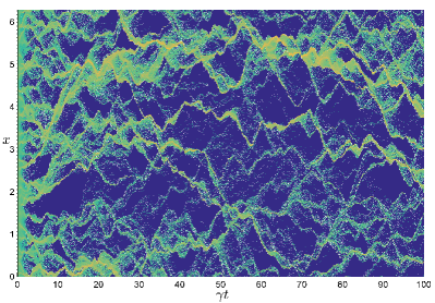
Figure 1: Trajectories, $x(t)$, for the dynamical system described by Eq. (2) with $\xi=0.08$, $L=2\pi$, and the dimensionless parameter [cf. Eq. (9)] is $\epsilon=1.7678$.

2 Distribution of sensitivity to initial conditions

The tendency of the trajectories to exhibit converging behavior is illustrated in Fig. 2, which shows the cumulative probability, $\Pi$, for the finite-time Lyapunov exponent (FTLE) at long times. The FTLE at time $t$ for a trajectory starting at $x_{0}$ is defined by

$$z(t)=\frac{1}{t}\ln\,\left|\frac{\partial x_{t}}{\partial x_{0}}\right|_{x(0)=x_{0}},$$ (1)

where $x_{t}$ denotes position at time $t$. The expectation value of $z(t)$ in the limit as $t\to\infty$ is termed the Lyapunov exponent: $\Lambda=\lim_{t\rightarrow\infty}\langle z(t)\rangle$ (angular brackets denote ensemble averages throughout). When $\Lambda>0$, there is an almost certain exponential growth of infinitesimal separations of trajectories. For the example in Fig. 1, we have $\Lambda=0.075\,\gamma$, where $\gamma$ is a positive parameter of the model [cf. Eq. (2)]. Figure 2 shows that the cumulative probability distribution for $z$ is very broad: even at time $t=41/\gamma$, which is comparable to the duration of the trajectories shown in Fig. 1, the probability of $z$ being negative is as high as $0.25$. We shall see how this very broad distribution can be quantified.

It is usually assumed that when the highest Lyapunov exponent is positive, the long-term behavior of a system is inherently unpredictable because of exponential sensitivity to the initial conditions. However, the phenomenon illustrated in Figs. 1 and 2 indicates that there may be basins in the space of initial conditions which attract a significant fraction of the phase space, giving a final position which is highly insensitive to the initial conditions. If the initial conditions which are of physical interest lie within one of these basins, the behavior of the system can be computed accurately for a time which is many multiples of the inverse of the Lyapunov coefficient.

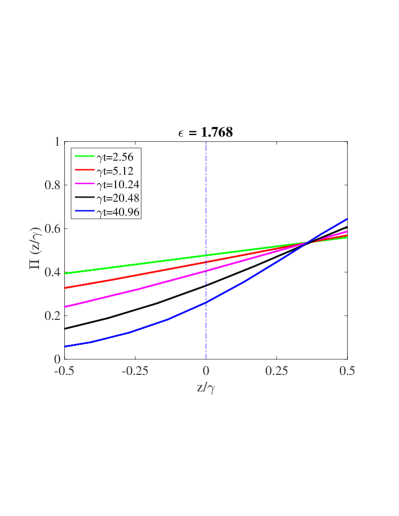
Figure 2: Cumulative probability, $\Pi$, for the value of the FTLE, $z(t)$, at different times (in dimensionless units). The distribution of $z(t)$ is very broad, even for large values of $t$. The parameters are the same as for Fig. 1.

Next we describe the equations of motion which were used to generate Fig. 1. They correspond to

$$\dot{x} = v,$$

$$\dot{v} = \gamma[u(x,t)-v],$$ (2)

where $x$ and $v$ are the position and velocity, respectively, of a small particle in a viscous fluid [7, 8]; $\gamma$ is a constant describing the rate of damping of the motion of a small particle relative to the fluid and $u(x,t)$ is a randomly fluctuating velocity field of the fluid in which the particles are suspended. In Fig. 1 we simulated a velocity field where the correlation function is white noise in time, satisfying $\langle u(x,t)\rangle=0$ and $\langle u(x,t)u(x^{\prime},t^{\prime})\rangle=\delta(t-t^{\prime})C(x-x^{\prime})$. The correlation function is $C(\Delta x)={\cal D}\xi^{2}\,\exp\left(-\Delta x^{2}/2\xi^{2}\right)$, where ${\cal D}$ and $\xi$ are constants. Trajectories which leave the interval $[0,L]$ are returned there by adding a multiple of $L$ to $x$. Equation (2) and related models have been studied intensively as descriptions of particles suspended in turbulent flows: see [9] and [10] for reviews.

3 Large-deviation analysis

In the large-time limit the probability density of $z$ is expected to be described by a large deviation approximation [11, 12]:

$$P(z)\sim\exp[-tJ(z)],$$ (3)

where $J(z)$ is termed the entropy function or the rate function. Large deviation methods have previously been applied to analyse the distribution of finite-time Lyapunov exponents in a variety of contexts: [13] and [14] are representative examples. In this Letter we are able to explain the broad distribution illustrated in Fig. 2 by determining the entropy function $J(z)$: if the second derivative, $J^{\prime\prime}(\Lambda)$, is small, the FTLE has a very broad distribution, giving a quantitative explanation for Fig. 2. In Fig. 3 we transform the empirical distributions of $z$ for different values of the time $t$ to determine the entropy function $J(z)$: the fact that the curves for different values of $t$ are quite accurately superimposed implies that the values of $t$ displayed in Fig. 2 are already sufficiently large for large deviation theory to be applicable. In Fig. 3 we also compare the entropy function obtained from our empirical distributions of $z$ with a theoretical curve (described below). There is very satisfactory agreement as $t\to\infty$, indicating that the effect illustrated in Figs. 1 and 2 has been understood quantitatively.

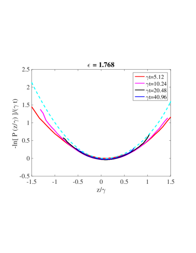
Figure 3: The transformed probability density function $-\ln\,P(z)/t$ approaches a limit, termed the large deviation entropy function $J(z)$. When $t\to\infty$, we find excellent agreement with a theoretical prediction for $J(z)$ (dashed line).

Our theoretical approach involves the analysis of a cumulant, $\lambda(k)$, which is defined by

$$\langle\exp(kzt)\rangle=\exp\left[t\lambda(k)\right].$$ (4)

The large deviation principle, as represented by equation (3), implies that

$$\langle\exp(kzt)\rangle=\int_{-\infty}^{\infty}{\rm d}z\ \exp[t(kz-J(z))].$$ (5)

A Laplace estimate shows that $\lambda$ and $J$ are a Legendre transform pair:

$$\lambda(k)=kz-J(z),\ \ \ J^{\prime}(z)=k.$$ (6)

For the model described by Eq. (2), the cumulant can be determined as an eigenvalue of a differential equation. Following the approach discussed in [15], we can obtain a Fokker-Planck equation for the variables $Y$ and $Z$ defined by $Z=\frac{\delta\dot{x}}{\delta x}$ and $Z=\dot{Y}$:

$$\frac{\partial\rho}{\partial t}=-\partial_{Y}(Z\rho)+\hat{\cal F}\rho,$$ (7)

where we have defined $\hat{\cal F}\rho\equiv\partial_{Z}(v(Z)\rho)+{\cal D}\gamma^{2}\partial_{Z}^{2}\rho$ with $v(Z)=-\gamma Z-Z^{2}$. Note that $Y=zt$, and we introduce the Lyapunov exponent, $\Lambda=\langle Z\rangle$. The cumulant $\lambda(k)$ is the largest eigenvalue of the operator $\hat{\cal F}+kZ$ [16]:

$$\hat{\cal F}\rho(Z)+kZ\rho(Z)=\lambda(k)\rho(Z)\ .$$ (8)

It is convenient to make a transformation of coordinates:

$$x=\left(\gamma{\cal D}\right)^{-1/2}Z\ ,\ \ \ \epsilon=\sqrt{\frac{{\cal D}}{\gamma}}\ ,\ \ \ E=-\frac{\lambda}{\gamma}\ .$$ (9)

The parameter $\epsilon$ is a dimensionless measure of the strength of inertial effects in the model (2). It is known that the Lyapunov exponent $\Lambda$ is negative, indicating almost certain coalescence of paths, when $\epsilon<\epsilon_{\rm c}=1.3309\ldots$ [17]. For $\epsilon>\epsilon_{\rm c}$, the Lyapunov exponent is positive so that the motion is chaotic. All of the illustrations in this paper are at $\epsilon=1.7678\approx 1.33\ldots\times\ \epsilon_{\rm c}$, where $\Lambda\approx 0.075\ \gamma$. In the coordinates defined by (9), the cumulant obeys an equation of the form

$$\partial_{x}(\partial_{x}+x+\epsilon x^{2})\rho(x)+k\epsilon x\rho(x)+E\rho(x)=0\ .$$ (10)

4 WKB method for cumulants

We now transform (10) so that it takes the form of a Schrödinger equation. Write $\hat{\cal F}=\partial_{x}[\partial_{x}+x+\epsilon x^{2}]$ and consider a transformation $\hat{\cal H}=\exp[-\Phi(x)]\hat{\cal F}\exp[\Phi(x)]$ with $\Phi(x)=-x^{2}/4-\epsilon x^{3}/6$. The cumulant $\lambda(k)$ is then obtained from the ground-state eigenvalue $E_{0}$ of a Hermitean operator

$$\psi^{\prime\prime}-V(x)\psi=E\psi$$ (11)

where $\lambda=-E_{0}/\gamma$ and the potential is

$$V(x)=\frac{1}{4}(x+\epsilon x^{2})^{2}-\frac{1}{2}-\epsilon(k+1)x\ .$$ (12)

Note that Eq. (11) corresponds to a Schrödinger equation with $m=\frac{1}{2}$ and $\hbar=1$. We remark that, when $\epsilon$ is small, the potential $V(x)$ has two minima, close to $x=0$ and to $x=-1/\epsilon$.

The WKB method [18, 19] provides a powerful tool for understanding the structure of solutions of the Schrödinger equation. It works best when the potential energy is slowly varying. In the case of equation (11), $\epsilon$ is the small parameter of WKB theory, because the minima of the potential move apart as $\epsilon\to 0$. In fact, a change of variable $x=\epsilon X$ formally reduces Eq. (11) to an expression where the $\psi^{\prime\prime}$ term has a small coefficient. We will find, however, that WKB methods yield surprisingly accurate results even when $\epsilon$ is not small. Define the momentum

$$p(x)=+\sqrt{V(x)-E},$$ (13)

with $p(x)=0$ where $V(x)<E$. The action integral is

$$S(x)=\int_{0}^{x}{\rm d}x^{\prime}\ p(x^{\prime}),$$ (14)

and define a pair of WKB functions

$$\phi_{\pm}(x)=\frac{1}{\sqrt{p(x)}}\exp[\pm S(x)]\ .$$ (15)

Then, as we get further away from turning points where $p(x)=0$, the solutions of (11) are asymptotic to a linear combination of WKB solutions $f(x)=a_{+}\phi_{+}(x)+a_{-}\phi_{-}(x)$, where $a_{\pm}$ are approximately constant, except in the vicinity of turning points where $E=V(x)$.

The Schrödinger equation (11) has unusual boundary conditions. The gauge transformation implies that the solutions of (10) and (11) are related by

$$\psi(x)=\exp[-\Phi(x)]\rho(x)=\exp\left[\frac{x^{2}}{4}+\epsilon\frac{x^{3}}{6}\right]\rho(x)\ .$$ (16)

Integration of equation (10) gives

$$\int_{-\infty}^{\infty}{\rm d}x\ (k\epsilon x+E)\rho(x)=0,$$ (17)

so that $\langle x\rangle$ must be finite. Then equation (16) implies that the coefficient of $a_{-}$ must be zero as $x\to-\infty$ (so that $\rho(x)$ does not diverge). Furthermore, $\rho(x)$ has an algebraic decay as $x\to\pm\infty$ and the coefficients of these algebraic tails must be equal in order for $\langle x\rangle$ to be finite. In terms of the coefficients $a_{\pm}$, the appropriate boundary conditions are therefore $\lim_{x\to-\infty}a_{+}=1$ and $\lim_{x\to-\infty}a_{-}=0$. At large positive values of $x$, we have

$$\lim_{x\to+\infty}\left\{\begin{array}[]{ll}a_{+}&=\exp(\Sigma)\\ a_{-}&=c\end{array}\right.$$ (18)

where $c$ is indeterminate, and where $\Sigma$ is defined by the finite limit of the following expression:

$$\Sigma=\lim_{x\to\infty}\left[S(x)-S(-x)-\Phi(x)+\Phi(-x)\right]\ .$$ (19)

We can determine the smallest eigenvalue $E(k)$ by using a shooting method to find a solution which satisfies (18). Solving numerically (11) amounts to propagating a two-dimensional vector $\mbox{\boldmath$a$}(x)=(\psi(x),\psi^{\prime}(x))$. We can take an initial condition for $x_{\rm i}$ large and negative in the form $\mbox{\boldmath$a$}_{\rm i}=\left(1,p(x_{\rm i})\right)\exp(\Phi(x_{\rm i}))$, corresponding to the asymptotic form of the solution which decays as $x\to-\infty$. We numerically propagate this solution for increasing $x$, and find that the solution increases exponentially. If the first element of the solution vector at $x_{\rm f}\gg 1$ is $a_{1}(x_{\rm f})=\psi(x_{\rm f})$, we can express the eigenvalue condition in the following form:

$$f(k,\epsilon,E)\equiv\frac{\psi(x_{\rm f})\exp[\Phi(x_{\rm f})]}{\psi(x_{\rm i})\exp[\Phi(x_{\rm i})]}=1\ .$$ (20)

This shooting method does provide very accurate values for the cumulant $\lambda=-\gamma E_{0}$. We used this method to obtain the cumulant. Performing a Legendre transform gives the theoretical curve in Figure 3. We remark that while the entropy function is well approximated by a quadratic, corresponding to the FTLE having an approximately Gaussian distribution for the parameter values reported here, our calculation can be used to accurately determine the non-Gaussian tails of the distribution of the FTLE.

5 Bohr-Sommerfeld quantisation for cumulant

It is also desirable to be able to make analytical estimates of the eigenvalues. The coefficients $a_{\pm}$ can be approximated as changing discontinuously when $x$ passes a turning point, where $E-V(x)$ is zero (or close to zero). Depending on the value of $E$ there may be one or two double turning points. We must take account of the fact that the amplitudes $a_{\pm}$ can change ‘discontinuously’ in the vicinity of turning points. Close to a double turning point, the equation is approximated by a parabolic cylinder equation

$$\frac{{\rm d}^{2}\psi}{{\rm d}x^{2}}-\frac{1}{4}x^{2}\psi+E\psi=0.$$ (21)

We are interested in constructing a solution which is exponentially increasing as $x$ increases, both when $x\to-\infty$ and for $x\to+\infty$. We can use this solution in the form $\phi(x)=A(x)\,\exp[S(x)]/\sqrt{p(x)}$ where $A(x)$ is asymptotically constant as $x\to\pm\infty$, and we take $A(-\infty)=1$. By adapting a calculation due to Miller and Good [20], we find that as $x\to+\infty$, the solution is approximated by $A(x)=F(E)$, where he function $F(E)$ is

$$F(E)=\frac{\sqrt{2\pi}}{\Gamma(\frac{1}{2}-E)}\exp[E(1-\ln\,|E|)],$$ (22)

and has zeros at $E=n+\frac{1}{2}$, $n=0,1,2,\ldots$. It approaches unity as $E\to-\infty$ and it oscillates approximately sinusoidally with amplitude equal to $2$ as $E\to+\infty$. Equation (22) can be used to determine the amplitude of the exponentially increasing solution after passing through a double turning point.

The eigenvalue condition (20) can also be expressed using the WKB approximation, leading to a generalisation of the Bohr-Sommerfeld quantisation condition. We consider cases where the potential has a closely spaced pair of real turning points, which will be treated as a double turning point, close to $x=0$. The effect of the double turning point is to cause the WKB amplitude of the exponentially increasing solution $\phi_{+}(x)$ to change by a factor $F(E)$, which we assume to be given correctly by the expression for a parabolic potential, Eq. (22). Because the potential is not precisely parabolic at the double turning point, the energy argument of $F(E)$ should be replaced by $F(\sigma/\pi)$, where $\sigma$ is a phase integral:

$$\sigma=\int_{x_{1}}^{x_{2}}{\rm d}x\ \sqrt{E-V(x)},$$ (23)

with $x_{1}$ and $x_{2}$ being the turning points where $E=V(x)$. This is the most natural choice of replacement variable, because it reproduces the standard Bohr-Sommerfeld condition in the case where the solution of the Schrödinger equation is square-integrable. In the more general case that we consider, the WKB eigenvalues are the solutions of

$$F(\sigma/\pi)\exp(\Sigma)=f$$ (24)

where $f=1$ corresponds to the correct boundary condition for our eigenvalue equation. Equation (24) is a generalisation of the usual Bohr-Sommerfeld condition, and it corresponds with the standard form of the Bohr-Sommerfeld criterion, which applies to bound-state problems, when $f=0$. We find that it does produce remarkably accurate eigenvalues, as illustrated in Fig. 4, despite that fact that $\epsilon$ is not small. In order to emphasise the fact that the modified Bohr-Sommerfeld condition does give very different eigenvalues, in Fig. 4 we display results for the conventional Bohr-Sommerfeld condition, $f=0$, as well as for $f=1$, which approximates the cumulant. We see that the modified Bohr-Sommerfeld condition provides accurate information about the cumulant $\lambda(k)$ in terms of two integrals of the momentum $\sqrt{V(x)-E}$, namely $\Sigma$ and $\sigma$.

We remark that Fyodorov et al have studied very closely related equations which occur in modelling pinning of polymers, including a related WKB analysis [21].

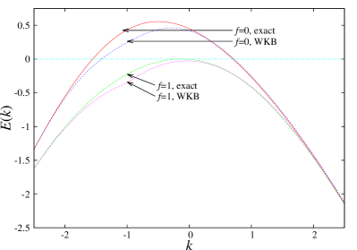
Figure 4: The generalised Bohr-Sommerfeld quantisation condition, Eq. (24), produces remarkably accurate eigenvalues. The upper curves are eigenvalues with the usual boundary condition (square-integrable wavefunction), with $f=0$, comparing the numerically exact eigenvalue with that obtained by the Bohr-Sommerfeld condition. The lower curves are for the criterion $f=1$ which applies to our cumulant eigenvalues. These data are for the case $\epsilon=1.7678$, and the dashed line in Fig. 3 is the Legendre transform of the numerically exact eigenvalue for $f=1$.

6 Conclusions

We have demonstrated, for the system described by Equations (2), that the usual definition of chaos, based on the instability of trajectories in the long time limit, does not preclude the existence of large islands of long term stability illustrated by the clustering of trajectories in Fig. 1. We argued that this clustering is related to the broad distribution of finite-time Lyapunov exponents, with a large probability of having negative values. In our analysis of Equations (2) we determined the cumulant, and performed a Legendre transform to obtain the large-deviation entropy function of the FTLE. We further showed how Bohr-Sommerfeld quantisation gives an accurate approximation to the cumulant. This analytical approach allows considerable scope for generalisation, for example to determine analytical approximations to the correlation dimension which describes the clustering of trajectories [22, 15]. We expect to explore this in a subsequent publication. We also anticipate that the methods will find quite direct application to clustering of particles advected on fluid surfaces, such as is seen in experiments reported in [23] and [24].

We should consider the extent to which the behaviour illustrated in Figure 1 is expected to be a general feature of chaotic dynamical systems. The differential structure of the equations of motion (2) has no properties which distinguish it from a generic dynamical system, and our argument was based upon considering the distribution of the FTLE, which has generic properties. In fact we can propose a simple criterion for observing the effect illustrated in Figures 1 and 2. We showed that the clustering is a consequence of there being a substantial probability to observe a negative FTLE at time $t$. Using Equation (3), and making a quadratic approximation for $J$, we have $P(z)\sim\exp[-tJ^{\prime\prime}(z-\Lambda)^{2}/2]$, which indicates that $P(0)$ is of order unity up to a dimensionless timescale given by:

$$t^{\ast}\Lambda=\frac{2}{J^{\prime\prime}(\Lambda)\Lambda}\ .$$ (25)

The natural expectation is that transient clustering may occur on a timescale such that $\Lambda t$ is of order unity. However, equation (25) indicates that the timescale over which transient clustering is observed may be much larger, and that $J^{\prime\prime}(\Lambda)/\Lambda$ is the relevant dimensionless measure of the clustering effect illustrated in Figure 1. This quantity diverges at the transition to chaos, and it may remain large even when the system is not close to a transition. For example, in Equations (2) we have $2/J^{\prime\prime}\Lambda\approx 13$ when $\epsilon/\epsilon_{\rm c}=1.33$. We remark that the dimensionless parameter in Eq. (25) can be expressed in terms of an integral of a correlation function:

$$t^{\ast}\Lambda=\frac{2}{\Lambda}\int_{-\infty}^{\infty}{\rm d}t\ \left[\langle Z(t)Z(0)\rangle-\Lambda^{2}\right]$$ (26)

where $Z(t)=\frac{{\rm d}}{{\rm d}t}\left[tz(t)\right]$. This expression can be useful in cases, such as Eq. (2), where it is practicable to write an equation of motion for $z(t)$ [22]. It is readily derived by estimating the variance of $tz(t)$.

Smith and co-workers (see [5, 4], and references cited therein) have emphasised the wide variability of the local instability of chaotic dynamical systems, indicating that the Lyapunov exponent is not sufficient to characterise chaos. Our work indicates that the transient stability can be very long-lived, and we propose that $1/J^{\prime\prime}\Lambda$ should be adopted as a parameter characterising the transient stability lifetime of chaotic systems. Our observation that trajectories of a generic chaotic system may be stable for surprisingly long times over a substantial domain of phase space implies in practice that small perturbations may not be amplified, making the system “predictable” longer than naturally expected. One potential application of this observation is to insurance or futures transactions, where someone takes a fee in exchange for writing a contract which requires a payment to be made if there is a loss or an unfavourable change in the price. The predictability of the behavior of the system over very long times for certain initial conditions, implied by our work, may be used to gain advantage. In some areas, such as weather-dependent risks, it may be possible to understand the conditions leading to a much smaller uncertainty than expected, so that the risk in a contract would be reduced. Finally, we remark that there are relations between our results and studies of the possibility of negative entropy production in systems out of equilibrium [25, 26]. The two processes are different because entropy is a property of phase-space volume, whereas the Lyapunov exponent describes distances between phase points. Whether the theoretical results developed in this context can lead to a better understanding of our system remains to be explored.

The authors are grateful to the Kavli Institute for Theoretical Physics for support, where this research was supported in part by the National Science Foundation under Grant No. PHY11-25915. We appreciate stimulating discussions with Arkady Vainshtein (on asymptotics and supersymmetry) and Robin Guichardaz (on large-deviation theory).

References

- [1] \NameOtt, E. \BookChaos in Dynamical Systems, 2nd edition \PublUniversity Press, Cambridge \Year2002
- [2] \NameFujisaka, H. \REVIEWProg. Theor. Phys.7019831264
- [3] \NameE. Aurell, E., Boffetta, G., Crisanti, A., Paladin, G. and Vulpiani, A. \REVIEWPhys. Rev. Lett.7719961262
- [4] \NameSmith, L. A., Ziehmann, C. and Fraedrich, K. \REVIEWQ. R. J. Meteor. Soc.12519992855-86
- [5] \NameSmith, L. A. \REVIEWPhil. Trans. Roy. Soc.3481994371-81
- [6] \NamePradas, M., Pumir, A, Huber, G. and Wilkinson, M. \REVIEWJ Phys A502017275101
- [7] \NameGatignol, R. \REVIEWJ. Méc. Théor. Appl.11983143-60
- [8] \NameMaxey, M. R. and Riley, J. J. \REVIEWPhys. Fluids261983883-9
- [9] \NameFalcovich, G., Gawedzki, K. and Vergassola, M. \REVIEWRev. Mod. Phys.732001913-75
- [10] \NameGustavsson, K and Mehlig, B. \REVIEWAdv. Phys.6520161-57
- [11] \NameFreidlin, M. I. and A. D. Wentzell, A. D. \BookRandom Perturbations of Dynamical Systems: Grundlehren der Mathematischen Wissenschaften \Vol260 \PublSpringer, New York \Year1984
- [12] \NameTouchette, H. \REVIEWPhys. Rep. 47820091
- [13] \NameTanase-Nicola, S. and Kurchan, J. \REVIEWJ. Phys. A: Math. and Gen.36200310299
- [14] \NameTailleur, J. and Kurchan, J. \REVIEWNature Physics32007203-7
- [15] \NameWilkinson, M., Guichardaz, R., Pradas, M. and Pumir, A. \REVIEWEurophys. Lett.111201550005
- [16] \NameDonsker, M. D. and Varadhan, S. R. S. \REVIEWCommun. Pure Appl. Math.2819761-47 \REVIEWCommun. Pure Appl. Math.281976279-301 \REVIEWCommun. Pure Appl. Math.291976389-461
- [17] \NameWilkinson, M. and Mehlig, B. \REVIEWPhys. Rev. E682003040101
- [18] \NameHeading, J. \BookAn Introduction io Phase Integral Methods \PublMethuen, London \Year1962
- [19] \NameLandau, L. D. and Lifshitz, E. M. \BookQuantum Mechanics \PublPergamon, Oxford \Year1958
- [20] \NameMiller, S. C. Jr. and Good, R. H. Jr. \REVIEWPhys. Rev.911953174-9
- [21] \NameFyodorov, Y. V., Le Doussal, P., Rosso, A. and Texier, C. arXiv:1703.10066.
- [22] \NameWilkinson, M., Mehlig, B., Gustavsson, K. and Werner, E. \REVIEWEur. Phys. J. B85201218
- [23] \NameSommerer, J. and E. Ott, E. \REVIEWScience3591993334
- [24] \NameLarkin, J., Bandi, M. M., Pumir, A. and Goldburg, W. I. \REVIEWPhys. Rev. E802009 066301
- [25] \NameGallavotti, G. and Cohen, E. G. D. \REVIEWPhys. Rev. Lett.7419952694
- [26] \NameSeifert, U. \REVIEWRep. Prog. Phys.752012126001