Machine learning techniques to select Be star candidates

Abstract

Context. Optical and infrared variability surveys produce a large number of high quality light curves. Statistical pattern recognition methods have provided competitive solutions for variable star classification at a relatively low computational cost. In order to perform supervised classification, a set of features is proposed and used to train an automatic classification system. Quantities related to the magnitude density of the light curves and their Fourier coefficients have been chosen as features in previous studies. However, some of these features are not robust to the presence of outliers and the calculation of Fourier coefficients is computationally expensive for large data sets.

Aims. We propose and evaluate the performance of a new robust set of features using supervised classifiers in order to look for new Be star candidates in the OGLE-IV Gaia south ecliptic pole field.

Methods. We calculated the proposed set of features on six types of variable stars and also on a set of Be star candidates reported in the literature. We evaluated the performance of these features using classification trees and random forests along with the K-nearest neighbours, support vector machines, and gradient boosted trees methods. We tuned the classifiers with a 10-fold cross-validation and grid search. We then validated the performance of the best classifier on a set of OGLE-IV light curves and applied this to find new Be star candidates.

Results. The random forest classifier outperformed the others. By using the random forest classifier and colours criteria we found 50 Be star candidates in the direction of the Gaia south ecliptic pole field, four of which have infrared colours that are consistent with Herbig Ae/Be stars.

Conclusions. Supervised methods are very useful in order to obtain preliminary samples of variable stars extracted from large databases. As usual, the stars classified as Be stars candidates must be checked for the colours and spectroscopic characteristics expected for them.

1 Introduction

In the last 30 years, several photometric surveys have been releasing huge amounts of data. This has motivated the use of statistical and computational techniques to process and analyse these large data sets (Bass (2016), Pichara et al. (2016), and references therein) and generate many catalogues of variable stars. Be stars are a particular class of variables, which despite more than 100 years of their discovery, evolutionary state, and dependency on metallicity are yet under study (Rivinius et al. 2013). For this reason, samples of Be stars in different environments are needed, and consequently, methods to classify the stars in a systematic way as well.

Debosscher et al. (2007) and Sarro et al. (2009) proposed using supervised learning methods to classify light curves of variable stars. This approach is a three-step process: representation, training, and evaluation. Light curves are represented with a set of features. These features can be categorical, discrete, or continuous parameters that are calculated for each light curve. They have to be informative enough to identify with high probability the variability class to which each light curve belongs. In the training step, a learning algorithm is used to infer, from available previously classified data (a training sample), a rule that assigns to each point of the feature space a variability type, that is, a classifier. Then, this rule can be used to classify light curves that have not been previously used in the training step. Finally, in the evaluation step, the performance of the resulting classifier is assessed on data that were not used in the training stage.

The selection of features is crucial because it is the only information available to the classifier. Debosscher et al. (2007) proposed using Fourier coefficients of light curves as features, finding that they could be used to classify classical Cepheids, Mira, RR Lyræ, among other variable stars. Deb & Singh (2009) performed principal component analysis on the interpolated values of magnitudes after folding the light curves using their periods. These authors found that the dimensionality of the representation of the light curves could be greatly reduced. Park et al. (2013) used the multi-scale visualisation technique, called thick-pen transformation, on the folded light curve to obtain features that can be used for classification. Kim et al. (2014) used a set of features that included the period of the light curves, quantities derived from Fourier decomposition, descriptive statistics of the magnitude density, and colour indexes. Despite the existence of efficient algorithms performing Fourier analysis, computing the Fourier coefficients is a demanding task for large data sets and the periods computed by automatic procedures often need to be checked manually.

Be stars are non-super giant very rapid rotators with spectral types between late O and early A, whose spectra at some time show or have shown one or more Balmer lines in emission, which are generated in a circumstellar decretion disk that emerges from the ejection of stellar mass whose causes are yet under study (Collins 1987, Rivinius et al. 2013). The decretion disk is conceptually different from the accretion disk that can be observed around young stellar objects such as Herbig Ae/Be (HAeBe) stars. The accretion disks are optically thick and feed a central young star.
Be stars show irregular spectroscopic and photometric variability. This behaviour is called the Be phenomenon. The most complete description of Be stars until now, including observations and models, has been presented by Rivinius et al. (2013). Photometric searches for Be star candidates (BeSC from hereafter) and the subsequent spectroscopic follow-up are useful to obtain samples of Be stars that allow us to analyse and prove different scenarios of the Be phenomenon. In particular, Mennickent et al. (2002) performed a photometric search for BeSC within the Small Magellanic Cloud (SMC) with the OGLE-II variable star catalogue. Those authors found that light curves of BeSC have morphologies similar to those of classical Be stars, but also they found other BeSC with completely different morphologies with diverse light curves. Based on the long-term morphology, those authors reported five types of variability: Type-1 stars are objects showing outbursts, some of which are characterised by a rise of brightness followed by a gradual decline lasting tens of days; and others are characterised by more symmetric rising and fading timescales, lasting hundreds of days. Their amplitudes are about 0.2 mag. The Galactic Be stars $\lambda$ Eri, $\mu$ Cen, and those stars reported by Hubert & Floquet (1998) and Hubert et al. (2000), exhibit this kind of variability. Type-2 stars show a brightness discontinuity or jump of the order of a few tenths of magnitudes that occurs on timescales of about few hundreds of days. This behaviour had never been observed in Galactic Be stars, as was also confirmed by Sabogal et al. (2014). Type-3 stars show periodic or quasi-periodic magnitude variations. Type-4 stars are objects with light curves showing stochastic magnitude variations, such as those exhibited by classical Be stars. Mennickent et al. (2002) also mentioned a group of BeSC light curves that showed brightness jumps and outbursts simultaneously. These stars were classified as Type1/2. Figure 1 shows examples of these morphological types. Sabogal et al. (2005) also found these morphological behaviour of BeSC in the Large Magellanic Cloud (LMC). Despite the diversity of the shape of their light curves, these stars are collectively classified as BeSC. Other light curve examples can be found in Mennickent et al. (2002) and Sabogal et al. (2014).

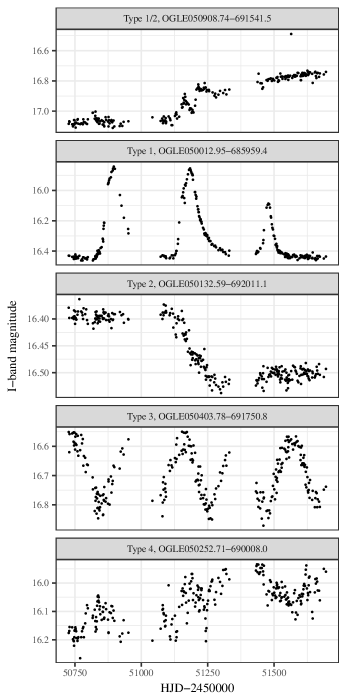
Figure 1: OGLE-II time series of LMC BeSC. Observations were sampled in a window close to 900 days.

Following the ideas of Sabogal et al. (2014), who used descriptive statistics of the magnitude density to search for BeSC, in this work we propose and evaluate a new set of features to classify variable stars and particularly BeSC. Since light curves sometimes contain atypical measurements, our descriptive statistics needs to be robust to the presence of such measurements. We train a set of state-of-the-art classifiers on a subset of six types of variable stars selected from OGLE-III and a set of BeSC to verify the usefulness of the features for performing classification of variables. Subsequently, we validate the resulting classifiers on a data set from the OGLE-IV database and use the best performing classifier to look for BeSC.

This article is organised as follows. In section 2, we describe the data used to train the classifiers. In section 3 we describe our features, the random forests classifier and classification trees. We only report the classification results for these two methods. For the sake of brevity of the main text, we defer the description of the other automatic classification techniques that we consider to the Appendix. In section 4, we show our results and discuss our findings of classification of variable stars using random forests and classification trees. In section 5 we present the results of applying the random forests method to classify BeSC from the OGLE-IV Gaia south ecliptic pole field catalogue (hereafter OGC). In section 6 we present a brief study of the infrared colours of our BeSC. Finally, in section 7 we present the main conclusions of this work.

2 Data

This work makes use of the variable star catalogues of the OGLE project, a long-term experiment whose main objective is searching for dark matter via gravitational lensing. This project began in 1992 and is in its fourth phase since 2010. The observations of this project have been made with the 1.3 m Warsaw telescope at Las Campanas Observatory in Chile. Characteristics of the new 32 chip mosaic camera and a technical overview can be found in Udalski et al. (2015).

Two OGLE data sets are used in this work. The first comes from OGLE-III and Sabogal et al. (2008). We use this data set to train and test our classifiers. The second comes from OGLE-IV. We use this data set to validate the best performing classifier. Within this last data set we also search for BeSC.

The OGLE-III data set consists of 432333 I band light curves (Udalski 2004) of variable stars belonging to the GB and Magellanic Clouds. These data cover about eight years from 2001 to 2009 (Udalski et al. 2015). From these data we select Cepheids (Ceph), $\delta$ Scuti ($\delta$ Sct), eclipsing binaries (EB), long period variables (LPV), RR Lyræ (RR Lyr), and type II Cepheid (T2Ceph) as our training sample. These variability classes and the number of stars in each class are shown in Table 1. Additionally, we selected the OGLE-III I band light curves of 475 BeSC reported by Sabogal et al. (2008) in the direction of the GB, and of 200 BeSC reported by Sabogal et al. (2005) in the LMC. These 675 BeSC are included in our training sample since they clearly exhibit the five morphological types shown in Figure 1.

Table 1: Training data set.

Variability	Location	Number	Total	References
type		of objects
BeSC	GB	475		1
	LMC	200	675	18
	GB	32		2
Ceph	LMC	3344	8006	3
	SMC	4630		4
$\delta$ Sct	LMC	2788	2788	5
EB	LMC	26121	32259	6
	SMC	6138		7
	GB	232406		8
LPV	LMC	91995	343785	9
	SMC	19384		10
	GB	16836		11
RR Lyr	LMC	24906	44217	12
	SMC	2475		13
	GB	357		14, 15
T2 Ceph	LMC	203	603	16
	SMC	43		17

(1) Sabogal et al. (2008); (2) Soszyński et al. (2011b); (3) Soszyński et al. (2008a); (4) Soszyński et al. (2010a); (5) Poleski et al. (2010); (6) Graczyk et al. (2011); (7) Pawlak et al. (2013); (8) Soszyński et al. (2013b); (9) Soszyński et al. (2009b); (10) Soszyński et al. (2011c); (11) Soszyński et al. (2011a); (12) Soszyński et al. (2009a); (13) Soszyński et al. (2010b); (14) Soszyński et al. (2011b); (15) Soszyński et al. (2013a); (16) Soszyński et al. (2008b); (17) Soszyński et al. (2010c); (18) Sabogal et al. (2005)

We applied the best performing classifier on the second data set, which consists of 6789 I band light curves. These light curves were reported and catalogued by Soszyński et al. (2012) in the study of OGLE-IV variable stars in the Gaia south ecliptic pole (GSEP) field. This work reported Ceph, $\delta$ Sct, EB, LPV, RR Lyr, and T2Ceph, as shown in Table 2. Stars showing variability with characteristics different to the mentioned classes, or showing similar characteristics with ambiguities, were assigned by Soszyński et al. (2012) to the class ”Other”, within this class 19 BeSC are reported. However, a visual inspection of the light curves belonging to the Other class suggests that the number of BeSC could be larger. For this reason we decide to look for BeSC in this data set.

Table 2: Gaia south ecliptic pole field OGLE-IV variables

Type	Ceph	$\delta$ Sct	EB	LPV	RR Lyr	T2 Ceph	Other
Number	135	159	1532	2799	686	5	1473

3 Set of features

In this section we describe what we mean by robustness; then we discuss our approach toward calculating robust quantities, describe our set of features, and visualise the data in the resulting feature space.

As OGLE variability studies are made principally in the I band, we compute the features only in that band. Our set of features carry information about the I band time series and are robust to the presence of outlying values, that is, their values do not change dramatically in the presence of such measurements as opposed to their non-robust counterparts. The robustness of a statistic is usually measured with the so-called breakdown point. This is the fraction of the data that needs to be contaminated before the statistic takes arbitrarily high (or low) values (see Huber & Ronchetti 2009, Chap. 1). We use the word “robust” in that sense throughout the document.

The approach we choose to calculate robust quantities is not the only approach in existence. One might be inclined to use a two-step process of first finding outlying values in the magnitude series and then applying classical estimates of parameters instead of their robust counterparts. We prefer the use of robust estimators for the following reasons. First, the process of automatic outlier identification in complex data is prone to false rejections and false retentions. For instance, popular outlying detection techniques could identify high magnitude values in the light curve of an EB system as outliers when they are not. Second, the process of screening for outliers and then applying classical statistical estimators to the remaining data usually requires the employment of robust estimators for the outlier identification step. Finally, robust estimation methods deal with outliers by appropriately down-weighting their effect on the resulting estimators. For a more detailed discussion, see Hampel et al. (1986) or Staudte & Sheather (1990).

In their study, Sabogal et al. (2014) used kurtosis and skewness. Kurtosis is a measure of both peakedness and tail weight. Skewness is the third standardised moment. In this work, we use the measure of skewness proposed by Brys et al. (2004), the octile skewness (OS) along with the measures of tail weight proposed by Brys et al. (2006), the left octile weight (LOW), and the right octile weight (ROW). We do not use the kurtosis and skewness because their calculation involve the third and fourth power of the deviation of the data points from the mean, which makes them very sensitive to outlying values. On the other hand the robustness of OS, LOW, and ROW comes from the robustness of quantile estimators. The OS is defined by

$$OS=\frac{(Q_{0.875}-Q_{0.5})-(Q_{0.5}-Q_{0.125})}{Q_{0.875}-Q_{0.125}},$$ (1)

where $Q_{p}$ is the p quantile of the magnitude distribution, that is, the value of $I$, such that the fraction $p$ of the values of I is smaller than $Q_{p}$. The OS is the difference between the lengths of the right and the left tails of the distribution scaled so that its maximum value is 1. It is positive for right-skewed distributions and negative for left-skewed distributions. Similarly,

$$LOW=\frac{(Q_{0.375}-Q_{0.25})-(Q_{0.25}-Q_{0.125})}{Q_{0.375}-Q_{0.125}},$$ (2)

and

$$ROW=\frac{(Q_{0.875}-Q_{0.75})-(Q_{0.75}-Q_{0.625})}{Q_{0.875}-Q_{0.625}},$$ (3)

describe how heavy the tail (left or right) of the distribution is relative to its magnitude near the centre of the distribution.

As estimators of location and scale we choose the median and the median absolute deviation (MAD), respectively. The median is $Q_{0.5}$ and MAD is defined by

$$MAD=\mathrm{median}_{i}(|I_{i}-\mathrm{median}_{j}(I_{j})|),$$ (4)

where $I_{i}$ is the $i$-th value of magnitude of the light curve in question. The $MAD$ is a measure of the dispersion of the magnitude distribution.

To measure the smoothness of the light curves, we choose a modified version of the Abbe value ($\mathcal{A}$) originally proposed by Von Neumann (1941) and later used by Mowlavi (2014) in the search of transients. The Abbe value is defined by

$$\mathcal{A}=\frac{n}{2(n-1)}\frac{\sum_{i=1}^{n-1}(I_{i+1}-I_{i})^{2}}{\sum_{i=1}^{n}(I_{i}-\overline{I})^{2}}$$ (5)

and compares the quadratic increments $(I_{i+1}-I_{i})^{2}$ with the standard deviation of the light curve. The $\mathcal{A}$ tends to one for a purely noisy light curve and to zero when the light curve shows a high degree of smoothness. In the case of periodic curves, when the sampling frequency is small with respect to the frequency of the curve, the light curve looks random before being folded and the Abbe value is close to one. This means that in this case the Abbe value does not reflect the smoothness of the folded curve, which is a limitation. On the other hand, for those curves whose variation patterns can be seen using the unfolded light curve, $\mathcal{A}$ is small. Since the quantities, $\overline{I}$, and $(I_{i}-\overline{I})^{2}$ are sensible to the presence of outlying values, we choose to modify this value by repeatedly using a robust measure of location instead of averages. As robust measure of location we use the M estimator proposed by Huber (1964) and explained in Venables & Ripley (2013). For a set of points $y_{1},\dots,y_{N}$, Huber’s estimate of location is the point $x$ at which

$$\sum_{i=1}^{N}\rho\left(\frac{y_{i}-x}{MAD}\right)$$ (6)

is minimised for

$$\rho(x)=\begin{cases}-c&\mbox{if }x<-c\\ x&\mbox{if }|x|<c\\ c&\mbox{if }x>c,\end{cases}$$ (7)

where $MAD$ is the median absolute deviation of the $y_{i}$ and $c$ can be chosen freely. We use $c=1.5$, that is, we winsorise at $1.5$ of the MAD. The point $\mathrm{loc}_{i}(y_{i})$ at which equation (6) is minimised is often called a Winsorised mean, defined by

$$\mathrm{loc}_{i}(y_{i})=\operatorname*{arg\,min}_{x}\sum_{i=1}^{N}\rho\left(\frac{y_{i}-x}{MAD}\right)$$ (8)

in the statistical literature. We then propose as measure of smoothness the modified Abbe value (MAV)

$$MAV=\frac{1}{2}\>\frac{\mathrm{loc}_{i}((I_{i+1}-I_{i})^{2})}{\mathrm{loc}_{i}((I_{i}-\mathrm{loc}_{j}I_{j})^{2})},$$ (9)

which has properties similar to those of $\mathcal{A}$. In figure 2, we compare two light curves with different values of $MAV$.

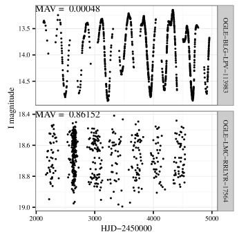
Figure 2: Time series of two variable stars from the OGLE-III catalogue. Upper panel shows LPV data with low MAV value, corresponding to curves that vary in the same timescale as the measurements. Bottom panel shows RR Lyr data with a higher MAV value that looks random before being folded.

The proposed feature statistics, i.e. the median, OS, LOW, ROW, MAD, and MAV combine robustness with the ability to measure the skewness, tail weight, location, scale, and smoothness of the light curves. In the case of OS, LOW, and ROW, their breakdown value is $12.5\%$, while that of the MAD and the median is $50\%$, which is the highest possible. In the case of OS, LOW, and ROW, we find that this level of robustness is enough for our purposes since it is rare to find light curves with such high levels of contamination. Other quantities with a higher breakdown point would result in less sensibility to distributional changes in tail weight and skewness (Brys et al. 2004, 2006).

Table 3: Statistical features

Measurement	Robust quantity
Location	Median
Scale	Median absolute deviation (MAD)
Skewness	Octile skewness (OS)
Tail weight	Left octile weight (LOW)
	Right octile weight (ROW)
Smoothness	Modified Abbe value (MAV)

In order to visualise how the data look in in the resulting six-dimensional feature space, we use the t-distributed stochastic neighbour embedding (t-SNE) (Van der Maaten & Hinton 2008). This is a non-supervised visualisation technique (it does not use the class to which each point belongs) that seeks to embed the six-dimensional data in the plane. This is carried out by minimising a loss function that captures the discrepancy between the high-dimensional and the two-dimensional structure. This procedure only involves one free parameter, called perplexity, which is to be set by the user. The perplexity is a continuous measure of how many neighbours of each point are taken into account. Figure 3 shows a t-SNE plot of the data used for training and Figure 4 shows a t-SNE plot of the data from OGLE-IV GSEP field. We built these figures via the Rtsne package (Krijthe 2015) for R and a perplexity value of $40$. The data set used for Figure 3 is a random sample that consists of either all or 2000 points of each variability class. This sample was subsampled further to avoid overplotting. In this plot it can be readily seen that light curves of the same variability class cluster together and that there is overlap between light curves from different classes that have similar light curves, for example T2Ceph and Ceph. The structure of this plot is robust to the choice of random sample.

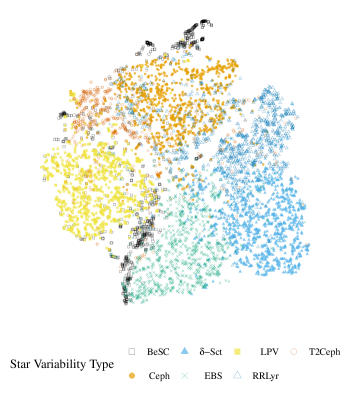
Figure 3: Visualisation of the six-dimensional feature space by t-SNE technique. The axes are omitted because the scale and orientation of this embedding carries no meaning. It can be seen how the different variability classes are separated in the six-dimensional feature space, although some overlapping of the classes is also evident.

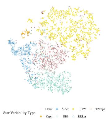
Figure 4: t-SNE visualisation of the OGC data. The axes are omitted because the scale and orientation of this embedding carries no meaning.

3.1 Method for classifier performance evaluation and parameter selection

Each classifier considered has one or more parameters that need to be tuned to maximise their performance. For each classifier, we performed a grid search on the classifier parameter space, that is, for each point in a grid of parameters, we estimated the performance and then chose one classifier. In this section we describe the procedure that we used to estimate the performance of the classifiers. We used normalised confusion matrices to prevent the imbalance in the number of light curves that belong to each class from affecting the performance measures. For more information on model selection via repeated cross-validation, Hastie et al. (2009) can be consulted.

We use 10-fold cross-validation and normalised confusion matrices to estimate the performance of the models that we consider. We randomly divided the data into 10 parts, called folds, with roughly the same number of examples, using stratified random sampling so that each fold had the same proportion of light curves of each variability class. For each fold, standard cross-validation was performed. This means that in each iteration the data on the fold were used as a hold-out sample on which a classifier trained with the remaining data was tested. In each iteration we cross-tabulated the observed and predicted classes for all light curves in the fold. This cross-tabulation is called (un-normalised) confusion matrix. We call the confusion matrix for the k-th iteration $C^{(k)}$. This is a table where each column represents the instances of the class to which each light curve belongs, while each row represents the class to which the classifier assigned it. This means that the entry $C_{ij}^{(k)}$ of the confusion matrix $C^{(k)}$ is the number of elements of the class $j$ that were classified as belonging to the class $i$ in the k-th cross-validation iteration. Thus, the cases in the diagonal are those that are classified correctly, while the cases outside the diagonals show the number of times that each possible error occurred. We normalised the confusion matrix so that each column sums up to one for reasons that we now explain.

Since the data that we used are surely not representative of the star populations that are observed, the use of the un-normalised confusion matrix can lead to misleading results. For instance, one common performance metric is the accuracy, which gives the proportion of light curves that are correctly classified. This can be the wrong measure of performance because of the imbalance in the number of members in each class. For example, if a classifier decided that all light curves of our sample are LPV, it would have almost 80% accuracy in our sample simply because of the over-representation of that variability class. Such a classifier achieves a relatively high accuracy but is not of practical use. Two other popular measures of performance are recall (also called sensitivity) and precision (also called positive predictive value). Recall is the proportion of light curves that are correctly classified, given that the light curves belong to a particular variability class. For the l-th class and the k-th cross-validation iteration, the recall is

$$\textrm{recall}_{l}^{(k)}=\frac{C_{ll}^{(k)}}{\sum_{i}C_{il}^{(k)}},$$ (10)

and precision is the fraction of light curves that are correctly classified given that the light curves are classified as belonging to a particular variability class. For the l-th class and the k-th cross-validation iteration, the precision is

$$\textrm{precision}_{l}^{(k)}=\frac{C_{ll}^{(k)}}{\sum_{j}C_{lj}^{(k)}}.$$ (11)

The cross-validation estimate of recall is

$$\textrm{recall}_{l}=\frac{1}{10}\sum_{k}\textrm{recall}_{l}^{(k)}$$ (12)

and is an estimator of the conditional probability of correct classification given that a light curve belongs to a variability class, while the cross-validation estimate of precision is

$$\textrm{precision}_{l}=\frac{1}{10}\sum_{k}\textrm{precision}_{l}^{(k)}$$ (13)

and is an estimator of the posterior probability of a light curve belonging to a particular class given that it is classified as such. While recall is not affected by the unrepresentativeness of our sample, precision is thus affected. For instance, if just 1% of LPV light curves were classified by a hypothetical model as BeSC and no other element of other class is wrongly classified as such, BeSC precision would drop to 12% when all BeSC light curves are correctly classified just because of the large number of LPV light curves in our sample. To avoid this and because the real proportion of objects belonging to each class in the observed fields is unknown, we normalised the confusion matrices by setting the population of each class to one, so that each column of the confusion matrices sums up to one. This is, if we call $\widehat{C}^{(k)}$ the normalised confusion matrix in the k-th fold, then

$$\widehat{C}^{(k)}_{ij}=\frac{C_{ij}^{(k)}}{\sum_{i}C_{ij}^{(k)}}.$$ (14)

We estimated precision, and recall analogues of equations (10) to (13) using normalised confusion matrices. This can be shown to lead to consistent estimates of the class conditional and posterior probability of correct classification (see appendix A), when the a priori probabilities of the different variability classes are all equal, that is, when the a priori distribution of the classes is uniform.

Ideally, a model should achieve perfect recall and precision for each class, but in practice it is found that there is a trade off between these two quantities when tuning parameter models: a compromise should be achieved. For this purpose, we use the mean $F_{1}$ score. For each class, the F1 score is defined as the harmonic mean of the precision and the recall

$$F_{1,l}=\frac{1}{\frac{1}{\textrm{precision}_{l}}+\frac{1}{\textrm{recall}_{l}}}=2\>\frac{\textrm{precision}_{l}\times\textrm{recall}_{l}}{\textrm{precision}_{l}+\textrm{recall}_{l}}.$$ (15)

The corresponding estimator from the k-th cross-validation iteration is

$$F_{1,l}^{(k)}=2\>\frac{\textrm{precision}_{l}^{(k)}\times\textrm{recall}_{l}^{(k)}}{\textrm{ precision}_{l}^{(k)}+\textrm{recall}_{l}^{(k)}}.$$ (16)

The mean (over the variability classes) F1 score for the k-th fold is

$$\overline{F}_{1}^{(k)}=\frac{1}{7}\sum_{l}F_{1,l}^{(k)}$$ (17)

and, finally, the cross-validation estimator of the mean F1 score is

$$\overline{F}_{1}=\frac{1}{10}\sum_{k}\overline{F}_{1}^{(k)}.$$ (18)

In the case of tree-based algorithms, in which the parameters of the classifier control their complexity, we choose the simplest model whose cross-validation estimate of the mean $F_{1}$ score is within one standard deviation (over the folds) of the highest value (Hastie et al. 2009, Chap. 7). This is carried out because simpler models are preferred and, in this case, the performance of the best and the simplest model cannot be statistically distinguished.

3.2 Classification trees and random forests

In this subsection we discuss in certain detail the random forest (RF) classifier, which achieved the best performance in our evaluation. We also describe classification trees (CT), which is necessary to understand random forests. Other classifiers considered in our study are described in Appendix B. All of the classifiers considered are non-linear, state-of-the-art classifiers, which are described, for instance, in Hastie et al. (2009). We use implementations of the classifiers in the R-statistical computing environment (R Core Team 2015), and the wrapper and other useful functions provided in the classification and regression training (caret) package (Khun 2016). Parameters for each classifier are tuned up following the process described in the previous subsection.

3.2.1 Classification trees

Classification trees were first proposed by Breiman, Friedman, Stone, and Olshen throughout several works that were later summarised by Breiman et al. (1984). The decision rule is implemented in the form of a binary decision tree. At each node a simple question is asked about one feature, and at the terminal nodes, a class is assigned to each example. In the case of numerical features $x_{i}$, these questions are of the form $x_{i}\leq c$ for constants $c$ that are chosen during the training step. These trees are constructed from the root by successively dividing the data using binary questions that maximise the reduction of a measure of “impurity”, that is, the diversity of classes in the resulting nodes. This process of successive division is repeated until each node contains only a predefined minimum number of examples or until they are pure. The resulting tree is usually large and, in order to avoid over fitting the data, it is then trimmed to reduce its complexity and improve its general properties. The resulting tree can be interpreted easily, since the divisions in the feature space give insight to the characteristics of the light curves.

We used the implementation of CT provided in the rpart package (Therneau et al. 2015). In this implementation, a complexity parameter (cp) needs to be tuned. It is the minimum decrease in the re-substitution estimate error that each partition has to achieve. The re-substitution estimate of the tree error is obtained from the proportions of the data classes at the terminal nodes and the a priori probability of each class (Breiman et al. 1984), which we chose to be uniform.

3.2.2 Random forests

Random forests were proposed by Breiman (2001) based on the idea that a set of weak classifiers can vote to conform a strong robust classifier. This method consists of building a large number of classification trees whose decisions are not very correlated and then taking the majority vote among them as the decision of the random forest. Each classification tree is built with a random sample taken with replacement from the complete learning sample (bootstrap sampling) using a random subset of a fixed size of features to reduce the correlation among trees. Each of the trees considered may over fit the data, but the ensemble does not, so pruning becomes unnecessary. Nevertheless, smaller trees may be grown by limiting their size. Thus, only the number of features that are randomly chosen for each tree, the total number of trees, and their size need to be tuned. Biau et al. (2008) showed that the decision rule given by random forests converges to the best possible decision rule for a given set of features when the size of the training set $N\to\infty$.

We used the implementation of RF provided in the randomForest package (Liaw & Wiener 2002). We tuned the number of trees (ntree), the maximum number of nodes of each tree (max_nodes), and the number of features randomly chosen for each tree (mtry).

4 Results and discussion

For CT and RF, the two classifiers performing best, we report the normalised confusion matrix, which we estimate using 10-fold cross-validation. We also report the cross-validation estimates of the recall and precision for each class with their cross-validation standard deviation (CV SD), that is, their standard deviation over the folds. In Table 4, we report the estimates of the mean $F_{1}$ scores for the five classifiers considered. We find the RF classifier to achieve the best performance.

In general, the decisions of the classifiers are not related in a simple manner. For classifiers with similar performances, their decisions are usually correlated. This happens because in some regions of feature space, where there are predominantly objects of one class, most well-performing classifiers agree on their decision, while in other regions, where there exists a mixed proportion of objects belonging to different classes, the performance of a classifier depends heavily on the complexity and shape of the decision boundary that they can learn. At the same time, the shape of the decision boundaries depends on the sample size and parameter choice. When comparing RF and CT, we find that they agreed on 93% of the sample. The majority of these stars are LPV objects, where both classifiers perform well. In the case of T2Ceph objects, where CT perform better than RF, 84% of the objects correctly classified by CT are also correctly classified by RF, and in the rest of classes, the agreement is higher than 94%.

Now we give a description of tuning and preprocessing steps that we follow CT and RF, as well as a brief discussion of their performance. We also present the results of applying the RF classifier to the Other sample in the OGC.

Table 4: Mean $F_{1}$ scores of the tuned classifiers.

Classifier	Mean $F_{1}$ Score	CV SD
Random forests	0.86	0.01
Classification trees	0.81	0.01
Gradient boosted trees	0.75	0.02
Support vector machines	0.72	0.02
K-nearest neighbours	0.65	0.01

4.1 Classification trees

We assessed the performance of CT with uniform prior on four values of the complexity parameter, i.e. $cp=0.1,0.01,0.001,0.0001$ (see section 3.2.1). We finally set the complexity parameter to 0.001 because lowering this parameter further than this does not bring statistically significant improvements and drastically increases the complexity of the resulting trees. In Table LABEL:table:resultsClassificationTrees we show the performance of the resulting classifier. The CT classifier offers a good compromise in terms of recall and precision, when compared to other classifiers, with the exception of RF. Ceph, RR Lyr, and T2 Ceph objects are classified with low recalls and sensitivities, but they are mainly confused between each other because the light curves of these objects are very similar.

Table 5: Cross-validation results of classification trees.

	Reference
Prediction	BeSC	Ceph	$\delta$Sct	EBS	LPV	RRLyr	T2Ceph
BeSC	0.93	0.02		0.02	0.02		0.01
Ceph	0.01	0.77				0.18	0.13
$\delta$Sct		0.01	0.89	0.06		0.03
EBS	0.01	0.02	0.05	0.86	0.01	0.03	0.04
LPV	0.04	0.01		0.02	0.94		0.06
RRLyr		0.05	0.04	0.01		0.69	0.06
T2Ceph	0.01	0.13	0.00	0.02	0.03	0.06	0.70
Recall	0.93	0.77	0.89	0.86	0.94	0.69	0.70
CV SD	0.03	0.02	0.02	0.01	0.01	0.01	0.08
Precision	0.93	0.70	0.90	0.84	0.87	0.81	0.74
CV SD	0.02	0.03	0.01	0.03	0.03	0.03	0.02
Number	675	8006	2788	32259	343785	44217	603

4.2 Random forests

We used a uniform prior and assess the performance of this method on five values of the number of features randomly selected for each tree, $mtry=2,3,4,5$ and grew a forest with 100, 200, and 500 trees without pruning. We find that different values of $mtry$ do not affect the performance of the method and that growing more than 200 trees does not have a significant effect on our performance metrics. Results for unpruned trees were not satisfactory, so we modified the maximum number of terminal nodes max_nodes that each tree in the forest could have. Since in the previous experiments the values of mtry did not affect the performance of the model, we fixed mtry to 2, and tried 10 values of max_nodes: $2^{1},2^{2},\dots,2^{10}$ while ntree was held fixed at 200. The maximum mean $F_{1}$ score was achieved at max_nodes$=2^{9}$ and max_nodes$=2^{10}$. We set the maximum number of nodes to $2^{9}$ and obtained the results shown in Table LABEL:table:resultsRandomForestMN9. This model achieved a better overall performance with recall/precision of 0.92/0.97 for BeSC objects; 0.91/0.91 for $\delta$-Scuti objects; 0.99/0.86 for LPV objects. Sensitivities for RRLyr, T2Ceph, and Ceph are lower than in the case of CT, but these classes were again confused among them. Additionally, since the maximum number of nodes max_nodes is smaller than that of unpruned trees, computation time and the memory needed is reduced.

Table 6: Cross-validation results of random forest. Each tree has a maximum number of nodes equal to $2^{9}$.

	Reference
Prediction	BeSC	Ceph	$\delta$Sct	EBS	LPV	RRLyr	T2Ceph
BeSC	0.92			0.01
Ceph	0.01	0.91	0.01			0.20	0.16
$\delta$Sct			0.91	0.05		0.04
EBS	0.02	0.01	0.05	0.89		0.02	0.03
LPV	0.04	0.01		0.02	0.99		0.09
RRLyr		0.02	0.03	0.01		0.72	0.06
T2Ceph	0.01	0.04	0.00	0.01		0.03	0.66
Recall	0.92	0.91	0.91	0.89	0.99	0.72	0.66
CV SD	0.04	0.01	0.02	0.01	$\sim 10^{-3}$	0.01	0.06
Precision	0.97	0.71	0.91	0.87	0.86	0.85	0.88
CV SD	0.01	0.02	0.01	0.02	0.03	0.03	0.03
Number	675	8006	2788	32259	343785	44217	603

4.3 Validation on the OGLE-IV Gaia south ecliptic pole field data

Random forest is the classifier that achieved the best overall performance during the cross-validation process in the OGLE-III data. We trained a RF classifier using the complete OGLE-III data set and the optimal parameters found in Section 4.2. We tested the resulting classifier on the OGC obtaining the results shown in Table LABEL:table:resultsOGLEIV. Since the variability classes of the new test data do not coincide with those of the training data, only recall (the proportion of objects that belong to a specific class that are correctly classified) for the classes found in both data sets is reported. No information about the classification posterior distribution can be extracted. The lowest recall is achieved for EB and T2Ceph objects at 72% and 60%, respectively. In the sample there are only five T2Ceph objects and four are classified either as T2Ceph or Ceph, but because of the small number of examples of this class, this result needs to be interpreted with caution. Remarkably, the rest of the objects belonging to the rest of variability classes, Ceph, $\delta$Sct, LPV, and RRLyr, are correctly classified at rates higher than 90%. From the Other class, 108 objects are classified as BeSC, and of those, 19 are the objects that were identified previously as BeSC by Soszyński et al. (2012). Besides, our classifiers found that in the Other class there are EB, $\delta$Sct, and LPV as shown in Table LABEL:table:resultsOGLEIV.

Despite the differences between the OGC and OGLE-III data in time span ($\sim$8 yr versus $\sim$ 2.4 yr) and the average number of photometric points per stars in the I band ($\sim$100-3000 versus $\sim$ 340), these results suggest that our set of features can also be used in such situations. Also, the proportion of time series belonging to each class in the OGC is not similar to that of the OGLE-III data either, where the imbalance from an abundance of LPV objects is much larger, or to the uniform prior distribution used to train the RF classifier. These results suggest that the procedure of assigning a uniform prior distribution and our set of features may be well suited for this situation and that the over-representation of LPV objects can be effectively overcome with these procedures. Nevertheless, since we do not have any other sensible prior distribution to which to compare, further conclusions could not be reached.

The RF classifier assigns to each object the class most frequently selected by the trees that makes up the forest. Table 8 shows the size of that ”majority” in our RF classification of the OGC data, by giving the octiles of the percentages of trees choosing the assigned class. For instance, half of the time, the assigned class gets the vote of at least $96\%$ of the trees, while $87.5\%$ of the classifications are made with a majority of at least $57\%$ of the trees. In general, the assigned class is selected by an ample majority of trees, especially considering that the votes are split among seven different classes, in principle. The Other class, as reported by Soszyński et al. (2012), contains objects whose variability type could not be unambiguously determined. This class includes objects that resemble rotating spotted stars, BeSC, and other variables. Since the training stage of the RF classifier did not include objects with the characteristics of some of those stars, RF probably assigns an incorrect class to some of those stars. This is a shortcoming of applying the supervised learning methods.

Table 7: Results of the random forest classifier on the OGLE-IV data set.

	Reference
Prediction	Ceph	$\delta$Sct	EB	LPV	RRLyr	T2Ceph	Other
BeSC	1		21	3			108
Ceph	126	1	42		10	1	52
$\delta$Sct		146	209		9		316
EB		2	1110	2	13		676
LPV	1		105	2790		1	226
RRLyr	3	10	19		652		86
T2Ceph	4		26	4	2	3	9
Total	135	159	1532	2799	686	5	1473
Recall	0.93	0.92	0.72	0.99	0.96	0.60	-

Table 8: Octiles of the size of the majority in RF classification.

Octile	100	87.5	75	62.5	50	37.5	25	12.5
Majority Size (%)	24.5	57.0	77.5	90.5	96.0	98.5	99.5	$\sim$100

5 Looking for BeSC in the OGLE-IV Gaia south ecliptic pole field using random forests

A visual inspection of the light curves classified as Others by Soszyński et al. (2012) suggests the presence of additional BeSC in the Other sample than the 19 reported by the authors. Since the RF classifier achieved the highest $F_{1}$ score for BeSC objects among the five classifiers considered, we used to look for BeSC in this data set. Additionally, we trained a binary RF classifier that distinguished BeSC objects from non-BeSC objects using the OGLE-III data and an a priori probability of 0.5. In order to train this binary RF, we followed the same procedure that we used for training the multi-class RF classifier, but we do not report the results because of the following. By inspecting the position of the objects that were classified as BeSC by both classifiers in the colour-magnitude diagram compared to the rest of the OGC sample, we decided to select the multi-class RF for further analysis because we believe it to be less prone to produce false positives. The multi-class RF classifier selects 108 objects as BeSC, while the binary RF classifier selects 215 objects. The multi-class RF classifier recovers the 19 BeSC reported previously in the OGC, and both the multi-class and the binary classifiers coincide in selecting 100 objects as BeSC, of which 18 had been previously reported in the OGC.

Figure 5: OGC colour-magnitude diagram for about 6700 variable stars reported by Soszyński et al. (2012). Black points represent 108 stars selected as BeSC by our multi-class RF classifier. Median magnitudes are used instead of average magnitudes.

Figure 5 shows the colour-magnitude diagram of all variable stars with $(V-I)$ colours reported by Soszyński et al. (2012). The BeSC selected in this work using the multi-class RF classifier are highlighted as darker points on the diagram. Two distinct groups of stars classified as BeSC by our procedure can be identified in Figure 5. One of these groups have stars showing blue colours, as expected to Be stars. The other is located in the red giant branch, indicating that these stars could probably be slowly pulsating variables (SPV) or LPV, whose light curve morphologies are similar to these of Be stars but their colours are redder. In order to obtain a more reliable list of BeSC, we discard the stars with colours out of the expected range of colours for Be stars from those initially labelled as BeSC. Intrinsic colours for Galactic Be stars, including their typical infrared excess, has been reported to be $-0.35<(V-I)_{0}<0.8$ mag (Wisniewski & Bjorkman 2006). The GSEP field covers four OGLE-IV fields (Soszyński et al. 2012), three of which are located about 270 arc min from the centre of the LMC. We search for the colour excess values of these fields at the Galactic Dust Reddening and Extinction Archive. For three fields (LMC562, LMC563, and LMC570), a $E(V-I)$ value of 0.093 mag is reported. These values are not derived from the IRAS/COBE extinction maps, while a value of 0.068 mag, for the field LMC571, was obtained from these maps. We adopt 0.093 mag as the colour excess for all fields. Therefore, we select BeSC the stars within the colour range $-0.257<(V-I)<0.893$ mag as more reliable, obtaining a total of 50 stars.

Table 9: Catalogue of BeSC in the GSEP field. Single or double asterisk appended to the last column indicates the stars that had been classified in the OGC as BeSC or the stars with infrared colours consistent with those of the HAeBe stars, respectively.

ID	RA	Dec	V	(V-I)	Type
LMC562.19.8354	05:58:54.52	-67:12:00.4	16.916	-0.195	Type-1
LMC563.21.7054	05:54:11.13	-65:58:00.5	16.103	-0.156	Type-1*
LMC562.28.8855	05:56:36.44	-66:56:51.4	16.660	-0.134	Type-1
LMC562.11.9588	05:57:04.69	-67:31:03.2	16.357	-0.126	Type-1*
LMC562.14.124	05:52:19.95	-67:39:59.4	16.286	-0.122	Type-2
LMC562.14.10726	05:51:55.37	-67:31:07.9	16.874	-0.119	Type-1
LMC562.01.211	06:00:43.40	-67:58:14.4	16.608	-0.112	Type-1*
LMC562.24.11360	05:51:09.41	-67:12:14.0	16.483	-0.107	Type-1*
LMC562.13.11357	05:53:14.85	-67:34:10.2	15.551	-0.104	Type-1
LMC562.16.231	05:48:48.80	-67:43:37.8	16.918	-0.097	Type-1*
LMC562.27.92	05:59:07.72	-67:05:13.6	16.612	-0.091	Type-1*
LMC562.26.8110	06:00:52.74	-66:58:17.4	16.399	-0.089	Type-1*
LMC562.02.7937	05:58:49.19	-67:55:28.9	15.159	-0.085	Type-4
LMC562.06.10895	05:51:53.39	-67:48:51.0	18.126	-0.070	Type-1
LMC563.04.477	05:53:21.94	-66:47:34.0	17.478	-0.049	Type-4
LMC562.09.110	06:00:10.48	-67:38:31.9	16.535	-0.031	Type-1
LMC562.32.173	05:50:07.46	-67:05:56.6	16.407	-0.016	Type-4
LMC562.24.132	05:50:04.86	-67:22:33.3	15.721	-0.008	Type-1*
LMC562.13.11454	05:53:22.34	-67:29:13.2	15.983	0.006	Type-1/2*
LMC562.21.180	05:55:28.96	-67:26:44.3	16.894	0.025	Type-1*
LMC563.16.113	05:48:08.49	-66:31:02.6	16.883	0.042	Type-3
LMC562.13.106	05:53:17.60	-67:43:38.0	15.848	0.053	Type-3
LMC563.06.110	05:50:01.51	-66:46:23.4	16.340	0.063	Type-1/2*
LMC562.13.11442	05:53:24.01	-67:30:36.1	16.451	0.066	Type-2
LMC562.12.10123	05:55:32.53	-67:32:20.9	15.088	0.075	Type-4
LMC562.20.85	05:57:07.95	-67:25:42.9	15.749	0.088	Type-3
LMC562.15.132	05:50:21.21	-67:41:43.8	15.717	0.111	Type-1
LMC562.20.9119	05:57:20.00	-67:12:46.5	16.065	0.113	Type-1*
LMC563.30.7056	05:52:13.54	-65:41:11.4	16.455	0.116	Type-4
LMC562.01.7994	06:00:12.35	-67:47:04.3	15.558	0.133	Type-4
LMC562.03.8441	05:56:48.78	-67:49:57.0	15.518	0.150	Type-1
LMC562.24.11487	05:51:01.93	-67:15:24.0	16.631	0.187	Type-2
LMC562.04.125	05:56:02.78	-67:57:41.8	16.122	0.191	Type-1
LMC562.28.207	05:56:30.97	-67:04:51.3	17.171	0.197	Type-4
LMC562.15.11956	05:50:54.39	-67:29:25.9	15.190	0.282	Type-1*
LMC570.14.103	06:02:19.40	-67:01:48.9	15.634	0.304	Type-4
LMC571.20.3879	06:05:28.35	-65:20:06.9	17.623	0.366	Type-3
LMC562.11.87	05:57:19.89	-67:43:19.9	15.695	0.370	Type-2
LMC562.20.78	05:56:45.52	-67:26:52.2	15.216	0.451	Type-1*
LMC562.02.8135	05:59:12.24	-67:50:07.5	17.503	0.484	Type-2
LMC562.16.12173	05:48:19.89	-67:29:40.6	15.112	0.580	Type-1*
LMC563.04.129	05:53:57.47	-66:50:01.6	17.078	0.582	Type-2**
LMC563.17.142	05:59:42.70	-66:09:08.0	16.543	0.610	Type-1**
LMC562.07.11068	05:50:26.35	-67:51:52.0	15.056	0.697	Type-4
LMC562.25.11162	05:49:04.56	-67:14:09.4	15.029	0.723	Type-4
LMC570.26.70	06:10:52.24	-66:30:11.4	16.730	0.757	Type-4**
LMC562.27.90	05:59:08.13	-67:05:20.0	16.269	0.846	Type-3
LMC570.17.266	06:12:12.82	-66:46:06.0	17.330	0.849	Type-2**
LMC563.05.450	05:52:48.46	-66:47:56.5	16.519	0.877	Type-1
LMC562.13.103	05:53:44.69	-67:43:54.5	14.911	0.888	Type-1*

Table LABEL:table:catalog presents the catalogue of these BeSC. The first column gives the OGC ID and the second and third columns show the equatorial coordinates (J2000). The fourth column gives the I band magnitude of each star. The fifth column shows the (V-I) colour for each star (all of these data are taken from Soszyński et al. (2012)). The last column gives our classification of the light curves based on the morphological types described by Mennickent et al. (2002). The total number of stars of each of these types is shown in Table LABEL:table:num.

Table 10: Types of BeSC found in the OGLE-IV GSEP field.

Type-1	Type-2	Type-3	Type-4	Type-1/2
25	7	5	11	2

It is seen that the majority of the BeSC selected are Type-1 stars. This reflects the useful effect of considering the LMC BeSC subsample as part of the training sample: in our Galaxy the amount of outbursting stars is much smaller than in the LMC, but since the GSEP field is near the LMC centre ($\sim 5^{\circ}$), it is expected to find outbursting BeSC. It is also worth noting that the presence in our catalogue of objects showing a brightness discontinuity of magnitude (Type-2 stars). Again, since these objects are observed in the direction of the GSEP, it is more probable that they are members of the LMC than of the Galaxy, where this type of variability for BeSC has never been detected. Spectroscopic follow-up of these stars are needed to confirm their Be nature. Figure 6 shows the time series of the 50 stars selected using the random forests algorithm and the colour criteria.

A fraction of the stars discarded from those initially selected as BeSC by our random forest procedure are periodic stars, as reported by the OGC. This fact gives more evidence that they are actually SPV, LPV, or non-periodic variable stars. LMC562.32.265 and LMC562.23.11510 are between the stars discarded by the colour criterion. The light curves of these non-periodic variables had been shown in Soszyński et al. (2012, Fig. 7). They are very similar to these of Type-1 and Type-2 BeSC, but their (V-I) colours are redder than the expected for Be stars.

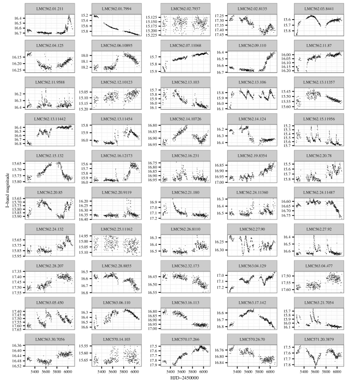
Figure 6: Time series of the selected 50 BeSC in the OGLE-IV Gaia south ecliptic pole field. Observations were sampled in a window close 900 days.

6 Infrared colours of the BeSC

Using 2MASS and WISE catalogues we explore the infrared properties of our selected sample of BeSC. Most of the 50 BeSC do not have reliable photometry in the 2MASS catalogue. Figure 7 shows the distribution of 15 BeSC in the 2MASS colour-colour diagram. About 8 BeSC have 2MASS colours with different levels of reddening. There are 4 stars (LMC563.04.129, LMC563.17.142, LMC570.26.70, and LMC570.17.266) that fall in the HAeBe region defined by Hernández et al. (2005) and have WISE colours consistent with HAeBe stars (Koenig 2014; Hernández et al. 2017). These stars are HAeBe candidates that could be surrounded by an optically thick accretion disk. The detection of HAeBe stars in the LMC has been reported previously (e.g. Hatano et al. 2006). Finally, there are 3 stars that fall below the HAeBe region (LMC562.13.11454, LMC562.26.8110, and LMC562.13.11454); these stars can be high mass objects (O type or early B) surrounded by a cool circumstellar envelope that produces excess at K band. Spectroscopic observations are necessary to reveal the nature of these objects. Despite the small sample of BeSC with infrared colours, apparently there is no relation between the morphological type of BeSC in table LABEL:table:catalog and the location on the 2MASS colour-colour diagram.

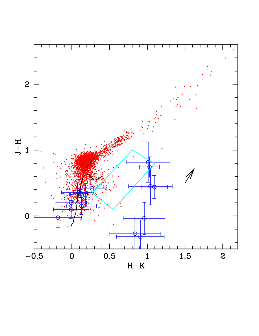
Figure 7: 2MASS colour-colour diagram for the variable stars (red dots) reported by Soszyński et al. (2012) and the 15 BeSC with 2MASS counterpart (blue open circles). The standard sequences from Bessel & Brett (1988) are shown in solid line (main sequence) and in dashed line (giant sequence). The loci of HAeBe stars is represented by the cyan box. Classical Be stars are located in the region near the blue end of the main sequence (Hernández et al. 2005). The arrow represents the reddening vector for 2 magnitudes of visual extinction.

7 Conclusions

In this work we presented and tested a new set of robust features for the supervised classification of variable stars and presented a new catalogue of 50 Be star candidates, four of which had infrared colours that were consistent with Herbig Ae/Be stars.

We presented a new set of features and showed their usefulness for the automatic classification of variable stars. This features are statistical parameters computed based on the I band magnitude density of the light curves that are robust to the presence of outliers. These parameters quantify the location, scale, skewness, tail weight, and smoothness of the magnitude density.

In order to prove the usefulness of our proposed set of features, we trained state-of-the-art classifiers on a sample of light curves from diverse variability types: Cepheids, $\delta$ Scuti, eclipsing binaries, long period variables, type II Cepheids, RR Lyræ, and Be star candidates. We tuned and tested the performance of classification trees and random forests along with K-nearest neighbours, support vector machines and gradient boosted trees via a grid search, 10-fold cross-validation, and the mean $F_{1}$ score based on normalised confusion matrices as performance metric. Our classifiers yielded correct classifications with high probability, which shows that our proposed set of features can be used to characterise different variability types. We found that the random forest classifier produces the best results.

We used the trained random forest classifier to look for Be star candidates in a subset of 1473 variable stars classified as Other in the OGLE-IV Gaia south ecliptic pole field field catalogue. After further selection using colour criteria, we present a new catalogue of 50 Be star candidates. Despite the necessity of a spectroscopic follow-up to confirm the presence of Balmer emission lines, and consequently the Be nature of these stars, their optical and infrared colours correspond to the expected for Be stars, except for four stars that have colours consistent with those of Herbig Ae/Be variables. Because there are BeSC in our selected sample showing in their light curves jumps or brightness discontinuities never observed in the Milky Way (Type 2 stars), this suggests that probably they belong to the Large Magellanic Cloud.

Appendix A Uniform prior probability, sensitivity, and specificity estimation

Here we show why the normalisation of the confusion matrix that we perform is equivalent to assigning a uniform a priori probability distribution to the observations of members of each variability class. First, we need to fix some notation. A classifier $g$ is a function that assigns to each vector $\@vec{x}$ a class $i\in\{1,\dots,M\}$. The value $P(\@vec{x},i)$ is the probability that a feature vector $\@vec{x}$ that corresponds to the class $i$ is observed. The recall seeks to estimate $P(g(\@vec{x})=i|i)$, and the precision $P(i|g(\@vec{x})=i)$ when the sample is representative of the object population. Since the sample considered in this work is surely not representative of the star populations, we need to assign subjectively a priori probabilities to the different variability classes. Because to our best knowledge there are no studies in this regard, we choose a uniform prior, that is, $P(i)=1/7$ for all classes. We can write in the case of uniform a priori probabilities

$$P(i|g(\@vec{x})=i)=\frac{P(g(x)=i|i)}{\sum_{j}P(g(x)=i|j)}.$$ (19)

For each $i$ and $j$ in the k-th iteration of the 10-fold cross-validation, we estimate $P(g(\@vec{x})=i|j)$ with

$$\hat{P}^{(k)}(g(\@vec{x})=i|j)=\frac{C_{ij}^{(k)}}{\sum_{k}C_{kj}^{(k)}},$$ (20)

where $C^{(k)}$ is the confusion matrix of the k-th holdout sample. The value $\hat{P}^{(k)}(g(\@vec{x})=i|j)$ is the $ij$ entry of the normalised confusion matrix, which we call $\hat{C}^{(k)}$. For the i-th class, the estimated recall for the k-th iteration, as given by 20, is just $\hat{C}^{(k)}_{ii}$. Our estimator of the precision in each iteration is

$$\hat{P}^{(k)}(i|g(\@vec{x})=i) =\frac{\hat{P}^{(k)}(g(x)=i|i)}{\sum_{j}\hat{P}^{(k)}(g(x)=i|j)},$$ (21)

$$=\frac{\hat{C}^{(k)}_{ii}}{\sum_{j}\hat{C}^{(k)}_{ij}}$$ (22)

which is the precision calculated with the normalised confusion matrix. Finally, our cross-validation estimators of $P(i|g(\@vec{x})=i)$, and $P(g(\@vec{x})=i|i)$ are just the average of the estimates over the folds, that is,

$$\hat{P}(i|g(\@vec{x})=i) =\frac{1}{10}\sum_{k}\hat{P}^{(k)}(i|g(\@vec{x})=i)$$ (23)

$$P(g(\@vec{x})=i|i) =\frac{1}{10}\sum_{k}\hat{P}^{(k)}(g(\@vec{x})=i|i).$$ (24)

Appendix B Other classifiers

B.0.1 K-nearest neighbours (KNN)

The KNN classifier was first proposed by Fix & Hodges Jr (1951) and republished by Silverman & Jones (1989). This algorithm is based on the observation that the examples of one class are close to each other and that it is possible to classify one example based on its nearest neighbours. Given a fixed integer, $k$, this rule assigns to each point in feature space the class to which the majority of its $k$ nearest neighbours belongs. It is possible to show that KNN converges to the best possible classification rule for a given set of features as the number of examples $N\to\infty$ as long as $k/N\to 0$. Despite its simplicity, KNN has been shown to be a competitive rule in the sense that it achieves accuracies comparable to those of more sophisticated decision rules, and only one parameter, the number $k$ of neighbours, needs to be tuned.

There exist weighted and bagged schemes of KNN. In weighting schemes, to each of the k nearest neighbours is given a different weight in the final decision. Bagging (short for bootstrap aggregating) consists of averaging the decision of several KNN classifiers trained with bootstrap samples of the original training sample, i.e. samples of the same size taken randomly with replacement from the original training sample. It has been shown that this reduces over-fitting and variance (Breiman 1996). Samworth (2012) showed that bagging is asymptotically equivalent to a weighted scheme and that there exists an optimal weighting scheme. We compare unweighted, optimal weighted (as shown by Samworth (2012)), and bagged KNN classifiers with the FNN package (Beygelzimer et al. 2013), which provides a fast implementation for these methods.
We scale the data so that each feature has standard deviation 1 and mean 0 and assess the performance of the model for 5 values: k = 1; 3; 5; 7; 9, finding that the best performance is achieved for low values of k and choose k = 1.

B.0.2 Support vector machines (SVM)

The SVM were first proposed by Cortes & Vapnik (1995) and a complete introduction to the topic can be found in Cristianini & Shawe-Taylor (2000). The SVM are binary classifiers that divide a transformed version of the feature space into two regions by finding the hyper-plane that separates data of both classes with maximal margin. Data are transformed hoping that in the high-dimensional space they are linearly separable. The maximal margin hyper-plane can be found by solving a convex optimisation problem for which efficient solvers are available and it includes a misclassification cost term that is controlled by a single parameter $C$. The transformation of the data into the high-dimensional space does not have to be known because the convex optimisation problem can only be solved by using the matrix of dot products in the high-dimensional space, which can be calculated directly using kernel functions. Consequently, the choice of kernel function is crucial for the performance of SVM. One of the most popular kernel functions is the radial basis kernel,

$$K(x,y)=e^{-\gamma\lVert x-y\rVert^{2}},$$ (25)

which has only one free parameter, $\gamma$. We tune the cost parameter $C$ and $\gamma$. In order to perform a $M$ class classification with SVM there are two popular approaches. The first one is called one-against-one and it consists of training $\frac{M(M-1)}{2}$ SVM that distinguish between each pair of classes. The final decision is to choose the class selected most often by the classifiers. The second one is called one-against-all and $M$ SVM are trained to distinguish between each class and the data non-belonging to that class. The decision is to select the class chosen by its classifier with the largest margin. One-against-one has proven to be faster and both approaches yield similar classification performances (Hsu & Lin 2002).

We use the interface to the libsvm implementation of SVM (Chang & Lin 2011) of the e1071 package (Meyer et al. 2015) and the wrapper function from the package caret.

Before adjusting the SVM, data are scaled so that each feature has a standard deviation of 1 and a mean of 0. The parameters $\gamma$ and C are selected by cross-validation as 0.04 and $2^{11}$, respectively. Candidates considered for $\gamma$ were equally spaced numbers between the reciprocals of the 0.1 and 0.9 percentiles of the interpoint distance distribution in the scaled feature space, while candidate values for C were powers of 2.

B.0.3 Gradient-boosted trees

Gradient boosting was proposed by Friedman (2001). In a similar fashion to random forests, it is based on the idea that a set of weak classifiers (classification trees) can be chosen to conform a strong classifier. In this case, each classification tree is built in a stagewise greedy manner, that is, each tree is built sequentially to maximise the decrease of a loss function associated with misclassification. During the training process, each tree is assigned different weight in the final decision of the classifier, whose final decision is the result of the weighted voting among the classification trees.

We use the implementation of the xgboost package (Chen et al. 2015) and several parameters need to be tuned. The learning rate, the number of trees, and their depth can be modified. The number of trees that are built is modified by the parameter nrounds. The learning rate modifies the contribution that each tree makes to the classifier and can be modified by changing between 0 and 1 the parameter eta. A smaller value eta makes the training more conservative, which means that a larger number of nrouds is needed. The depth of each tree is controlled by the parameter max_depth. We tune both nrouds and max_depth and left eta fixed to its default value of 0.3.

By grid search, the number of trees that are grown was set to nround = 100, while the maximum depth of the trees was chosen as max_depth=7.

References

- Bass (2016) Bass, G.and Borne, K. 2016, MNRAS, 459, 3721
- Bessel & Brett (1988) Bessel, M. S. & Brett, J. M. 1988, PASP, 100, 1134
- Beygelzimer et al. (2013) Beygelzimer, A., Kakadet, S., Langford, J., et al. 2013, FNN: Fast nearest neighbor search algorithms and applications., r package version 1.1
- Biau et al. (2008) Biau, G., Devroye, L., & Lugosi, G. 2008, The Journal of Machine Learning Research, 9, 2015
- Breiman (1996) Breiman, L. 1996, Machine Learning, 24, 123
- Breiman (2001) Breiman, L. 2001, Machine Learning, 45, 5
- Breiman et al. (1984) Breiman, L., Friedman, J., Stone, C. J., & Olshen, R. A. 1984, Classification and Regression Trees, 1st edn. (New York, N.Y.: Chapman and Hall/CRC)
- Brys et al. (2004) Brys, G., Hubert, M., & Struyf, A. 2004, Journal of Computational and Graphical Statistics, 13
- Brys et al. (2006) Brys, G., Hubert, M., & Struyf, A. 2006, Computational statistics & data analysis, 50, 733
- Chang & Lin (2011) Chang, C.-C. & Lin, C.-J. 2011, ACM Transactions on Intelligent Systems and Technology (TIST), 2, 27
- Chen et al. (2015) Chen, T., He, T., & Benesty, M. 2015, xgboost: Extreme Gradient Boosting, r package version 0.4-2
- Collins (1987) Collins, G. W. 1987, Physics of Be stars, ed. A. Slettebak & T. P. Snow, Proc. IAU Coll. 92 (Cambridge University Press)
- Cortes & Vapnik (1995) Cortes, C. & Vapnik, V. 1995, Machine Learning, 20, 273
- Cristianini & Shawe-Taylor (2000) Cristianini, N. & Shawe-Taylor, J. 2000, An introduction to support vector machines and other kernel-based learning methods (Cambridge University press)
- Deb & Singh (2009) Deb, S. & Singh, H. P. 2009, Astronomy and Astrophysics, 507, 1729
- Debosscher et al. (2007) Debosscher, J., Sarro, L. M., Aerts, C., et al. 2007, A&A, 475, 1159
- Fix & Hodges Jr (1951) Fix, E. & Hodges Jr, J. L. 1951, Discriminatory analysis-nonparametric discrimination: consistency properties, Tech. rep., DTIC Document
- Friedman (2001) Friedman, J. H. 2001, The Annals of Statistics, 29, 1189
- Graczyk et al. (2011) Graczyk, D., Soszyński, I., Poleski, R., et al. 2011, Acta Astron., 61, 103
- Hampel et al. (1986) Hampel, F. R., Ronchetti, E. M., Rousseeuw, P. J., & Stahel, W. A. 1986, Robust statistics: the approach based on influence functions (John Wiley & Sons)
- Hastie et al. (2009) Hastie, T., Tibshirani, R., & Friedman, J. 2009, The Elements of Statistical Learning, Springer Series in Statistics (New York, NY: Springer New York)
- Hatano et al. (2006) Hatano, H., Kadowaki, R., Nakajima, Y., et al. 2006, AJ, 132, 2653
- Hernández et al. (2005) Hernández, J., Calvet, N., Hartmann, L., et al. 2005, AJ, 129, 856
- Hernández et al. (2017) Hernández, J., Villareal, L., Calvet, N., et al. 2017, In prep.
- Hsu & Lin (2002) Hsu, C.-W. & Lin, C.-J. 2002, Neural Networks, IEEE Transactions on, 13, 415
- Huber (1964) Huber, P. J. 1964, The Annals of Mathematical Statistics, 35, 73
- Huber & Ronchetti (2009) Huber, P. J. & Ronchetti, E. M. 2009, Robust Statistics, 2nd edn. (Hoboken, N.J: Wiley)
- Hubert & Floquet (1998) Hubert, A. M. & Floquet, M. 1998, A&A, 335, 565
- Hubert et al. (2000) Hubert, A. M., Floquet, M., & Zorec, J. 2000, Proc. IAU Coll. 175, The Be Phenomenon in Early-Type Stars., ed. M. A. Smith, H. F. Henrichs, & J. Fabregat, Proc. IAU Coll. 92 (Astron. Soc. Pac.)
- Khun (2016) Khun, M. 2016, caret: Classification and Regression Training, , r package version 6.0-6.4
- Kim et al. (2014) Kim, D.-W., Protopapas, P., Bailer-Jones, C. A. L., et al. 2014, A&A, 566, A43
- Koenig (2014) Koenig, X. P. & Leisawitz, D. T. 2014, ApJ, 791, 131
- Krijthe (2015) Krijthe, J. 2015, Rtsne: T-Distributed Stochastic Neighbor Embedding using Barnes-Hut Implementation, r package version 0.10
- Liaw & Wiener (2002) Liaw, A. & Wiener, M. 2002, R News, 2, 18
- Mennickent et al. (2002) Mennickent, R. E., Pietrzyński, G., Gieren, W., & Szewczyk, O. 2002, A&A, 393, 887
- Meyer et al. (2015) Meyer, D., Dimitriadou, E., Hornik, K., Weingessel, A., & Leisch, F. 2015, e1071: Misc Functions of the Department of Statistics, Probability Theory Group (Formerly: E1071), TU Wien, r package version 1.6-7
- Mowlavi (2014) Mowlavi, N. 2014, A&A, 568, 78
- Park et al. (2013) Park, M., Oh, H.-S., & Kim, D. 2013, PASP, 125, 470
- Pawlak et al. (2013) Pawlak, M., Graczyk, D., Soszyński, I., et al. 2013, Acta Astron., 63, 323
- Pichara et al. (2016) Pichara, K., Protopapas, P., & León, D. 2016, ApJ, 819, 18
- Poleski et al. (2010) Poleski, R., Soszyński, I., Udalski, A., et al. 2010, Acta Astron., 60, 1
- R Core Team (2015) R Core Team, . 2015, R: A Language and Environment for Statistical Computing (Vienna, Austria: R Foundation for Statistical Computing)
- Rivinius et al. (2013) Rivinius, T., Carciofi, A. C., & Martayan, C. 2013, A&ARv, 21, 69
- Sabogal et al. (2014) Sabogal, B. E., García-Varela, A., & Mennickent, R. E. 2014, PASP, 126, 219
- Sabogal et al. (2005) Sabogal, B. E., Mennickent, R. E., Pietrzyński, G., & Gieren, W. 2005, MNRAS, 361, 1055
- Sabogal et al. (2008) Sabogal, B. E., Mennickent, R. E., Pietrzyński, G., et al. 2008, A&A, 478, 659
- Samworth (2012) Samworth, R. J. 2012, The Annals of Statistics, 40, 2733
- Sarro et al. (2009) Sarro, L. M., Debosscher, J., López, M., & Aerts, C. 2009, A&A, 494, 739
- Schlafly & Finkbeiner (2011) Schlafly, E. & Finkbeiner, D. 2011, ApJ, 737, 103
- Silverman & Jones (1989) Silverman, B. W. & Jones, M. C. 1989, International Statistical Review/Revue Internationale de Statistique, 57, 233
- Soszyński et al. (2011a) Soszyński, I., Dziembowski, W. A., Udalski, A., et al. 2011a, Acta Astron., 61, 1
- Soszyński et al. (2008a) Soszyński, I., Poleski, R., Udalski, A., et al. 2008a, Acta Astron., 58, 163
- Soszyński et al. (2010a) Soszyński, I., Poleski, R., Udalski, A., et al. 2010a, Acta Astron., 60, 17
- Soszyński et al. (2011b) Soszyński, I., Udalski, A., Pietrukowicz, P., et al. 2011b, Acta Astron., 61, 285
- Soszyński et al. (2013a) Soszyński, I., Udalski, A., Pietrukowicz, P., et al. 2013a, Acta Astron., 63, 37
- Soszyński et al. (2012) Soszyński, I., Udalski, A., Poleski, R., et al. 2012, Acta Astron., 62, 219
- Soszyński et al. (2010b) Soszyński, I., Udalski, A., Szymański, M. K., et al. 2010b, Acta Astron., 60, 165
- Soszyński et al. (2008b) Soszyński, I., Udalski, A., Szymański, M. K., et al. 2008b, Acta Astron., 58, 293
- Soszyński et al. (2009a) Soszyński, I., Udalski, A., Szymański, M. K., et al. 2009a, Acta Astron., 59, 1
- Soszyński et al. (2009b) Soszyński, I., Udalski, A., Szymański, M. K., et al. 2009b, Acta Astron., 59, 239
- Soszyński et al. (2010c) Soszyński, I., Udalski, A., Szymański, M. K., et al. 2010c, Acta Astron., 60, 91
- Soszyński et al. (2011c) Soszyński, I., Udalski, A., Szymański, M. K., et al. 2011c, Acta Astron., 61, 217
- Soszyński et al. (2013b) Soszyński, I., Udalski, A., Szymański, M. K., et al. 2013b, Acta Astron., 63, 21
- Staudte & Sheather (1990) Staudte, R. G. & Sheather, S. J. 1990, Robust estimation and testing, Wiley Series in Probability and Statistics (John Wiley & Sons)
- Therneau et al. (2015) Therneau, T., Atkinson, B., & Ripley, B. 2015, rpart: Recursive Partitioning and Regression Trees, r package version 4.1-10
- Udalski (2004) Udalski, A. 2004, Acta Astron., 53, 291
- Udalski et al. (2015) Udalski, A., Szymański, M. K., & Szymański, G. 2015, Acta Astron., 65, 138
- Van der Maaten & Hinton (2008) Van der Maaten, L. & Hinton, G. 2008, The Journal of Machine Learning Research, 9, 85
- Venables & Ripley (2013) Venables, W. N. & Ripley, B. D. 2013, Modern applied statistics with S-PLUS (Springer Science & Business Media)
- Von Neumann (1941) Von Neumann, J. 1941, The Annals of Mathematical Statistics, 12, 367
- Wisniewski & Bjorkman (2006) Wisniewski, J. P. & Bjorkman, K. S. 2006, ApJ, 652, 458