Quasiparticle interference in multiband superconductors with strong coupling.

Abstract

We develop a theory of the quasiparticle interference (QPI) in multiband superconductors based on strong-coupling Eliashberg approach within the Born approximation. In the framework of this theory, we study dependencies of the QPI response function in the multiband superconductors with nodeless s-wave superconductive order parameter. We pay a special attention to the difference of the quasiparticle scattering between the bands having the same and opposite signs of the order parameter. We show that, at the momentum values close to the momentum transfer between two bands, the energy dependence of the quasiparticle interference response function has three singularities. Two of these correspond to the values of the gap functions and the third one depends on both the gaps and the transfer momentum. We argue that only the singularity near the smallest band gap may be used as an universal tool to distinguish between $s_{++}$ and $s_{\pm}$ order parameters. The robustness of the sign of the response function peak near the smaller gap value, irrespective of the change in parameters, in both the symmetry cases is a promising feature that can be harnessed experimentally.

I Introduction

In recent decades, a number of new materials such as cuprates, magnesium diboride, chalcogenides and iron pnictides with a high critical temperature have been found. Hosono2008 ; Mazin02 ; Stewart11 ; Paglione10 ; Johnston10 ; Hosono15 This generated numerous proposals for the mechanisms of superconductivity and the symmetry of the order parameters. Cruz08 ; Hidenori09 ; Pratt09 ; Hirsch2016 The most recent findings are of iron-based superconductors (FeBS) having critical temperatures up to 100 KFeng2015 . The important issue of the pairing mechanisms and the symmetry of the order parameter in these materials is still a matter of an extensive debate. They, as shown by DFT calculations and confirmed by ARPES, are in-fact multiband materials with, either four or five, quasi-2D disconnected Fermi pockets. Singh2008 ; Kontani2015 The hole pockets are centred at $\Gamma=(0,0)$ and the electron pockets are centred at M=($\pi$,$\pi$). The nesting between the electron and hole pockets on the one hand leads to strong spin fluctuations, which favor $s_{\pm}$ superconductivity, with the order parameter having the opposite sign for the electron and the hole pockets.Johannes2008 ; McElroy2003 ; Mazin2010 ; Hirschfeld2011 ; Chubukov2008 On the other hand it may enhance orbital fluctuations, favoring s++ superconductivityHanaguri2010 , with the order parameter, having the same sign for the electron and the hole pockets. Therefore, such a sign change of the order parameter between the electron and hole pockets should hint at the possible pairing mechanism. Korshunov2011 ; Monthoux 2001 ; Golubov2008 ; Kuroki8 ; Kordyuk12 ; Werner2012 ; Chen2014

Even though the symmetry of the order parameter was determined for some of the representative of FeBS, e.g. in the inelastic neutron scattering experiments, it still does not give the complete picture for all compounds. The underlying reason is the multiband character of the Fermi surfaces in the FeBS. In this case the order parameter may change sign due to impurities; as it was demonstrated theoretically Efremov2011 ; Efremov13 ; Korshunov2014 and experimentally shilling2016 with doping either to d-wave symmetry Reid2012 ; Hafeiz2013 ; Grinenko2014 ; Grinenko20142 or change a sign Wang2016 . Therefore, a universal tool to ascertain the pairing symmetry is much needed. In contrast to high $T_{c}$ cuprates, phase-sensitive experiments using FeBS-based Josephson junctions have not been performed yet. The main difficulty for such a multiband superconductor is the need to design an experimental geometry in such an ingenious way, such that, the current through one contact is dominated by carriers having positive sign of order parameter and in the other contact the opposite case occurs. The isotropic nature of the s-wave fails the effort in this direction; however, the extended s-wave nature comes directly under the realm of such experimental investigation.Golubov2013 ; Mazin2009 ; Burmistrova2015 ; Golubov2009

One of the methods for resolving the symmetry of the order parameter, is the study of the local density of states (LDOS) modulations due to the quasiparticle interference (QPI), in the presence of impurities; which, could provide interesting information on the pairing symmetry of the gap function. The STM studies of conductance modulations have been utilized in earlier investigations as the direct probes of the quantum interference of electronic eigenstates in metalsCrommie1993 , semiconductorsKanisawa2001 and cupratesHoffman2002 ; Hanaguri2007 ; Howald2003 . In Fe-based superconductors, theoretical predictions for the dispersion of the QPI vector peaks have been made with models with electron and hole pockets for the case of $s_{\pm}$superconducting order.Coleman09 ; Skyora2011 ; Hirschfeld15 ; Scalapino2003 ; Scalapino2012

In view of the above discussion, it would be helpful to formulate a model for the QPI to reveal qualitative differences between the response in the $s_{\pm}$ and $s_{++}$ pairing states. In this work, we formulate such a model for multiband superconductors by employing the Eliashberg formalism which naturally takes into account the temperature and retardation effects. We discuss the temperature dependence of the QPI spectral function and emphasize upon the finite temperature effect on the distinction between the two symmetry cases viz. $s_{\pm}$ and $s_{++}$. We show, both analytically and numerically, that within the Born approximation, the quasiparticle interference response function given as the function of energy has three singularities. Two of these correspond to the values of the energy gaps and the third depends on both the gaps and the transfer momentum. We argue that only the lowest value in the energy singularity may be used as an universal tool for the determination of the phase shift of the order parameter between the bands. We identify the robustness of the sign of response function peak near the smaller gap value in both the symmetry cases is a promising feature that can be used to identify a pairing symmetry.

The paper is organized as follows. In section II we shortly introduce the main object of the present study, namely the QPI response function and the Eliashberg approach for the single-particle correlation functions in multiband systems with strong coupling interaction. The theoretical background to obtain the LDOS and the response function is explained in the section III. where, we numerically analyse the response function in strong coupling for inter- and intra-band case. In section IV, the general case of away from ideal nesting condition with non-zero band ellipticity $\epsilon$ and the shifted Fermi surface energy $\delta\mu$ is discussed. We show the dependence of QPI response function on the inherently present large momentum transfer process that could probe the sign-changing gap symmetry. In section V we conclude the paper with the summary of our results.

II The Eliashberg Approach

To find the single-particle correlation functions in multiband systems with strong coupling interaction we employ the Eliashberg approach Carbotte90 ; Scalapino66 ; Allen82 ; Marsiglio2008 ; Scalapino69 ; Maksimov82 ; Parker08 ; Vonsovskii82 . For the sake of simplicity, the consideration here is restricted by assuming the two bands scenario. The generalization for higher number of bands is straightforward. Since, the superconducting gap functions have weak momentum dependence, the systems like Fe-based superconductors can be successfully described in the frame of quasi-classical Green functions $\hat{\mathbf{g}}_{\alpha}(\omega)$:

$$\hat{\mathbf{g}}_{\alpha}(\omega)=N_{\alpha}(0)\int d\xi\hat{\mathbf{G}}_{\alpha}(\mathbf{k},\omega)$$ (1)

where $\alpha=a,b$ is the band index and and $N_{\alpha}(0)$ is the density of states. In the following, we will use retarded Green function throughout and therefore we shall omit the index R. In the Nambu notations the full Green functions have the form:

$$\hat{\mathbf{G}}_{\alpha}(\mathbf{k},\omega)=\frac{\tilde{\omega}_{\alpha}\hat{\tau}_{0}+\xi_{\alpha,\mathbf{k}}\hat{\tau}_{3}+\tilde{\phi}_{\alpha}\hat{\tau}_{1}}{\tilde{\omega}_{\alpha}^{2}-\xi_{\alpha,\mathbf{k}}^{2}-\tilde{\phi}_{\alpha}^{2}}$$ (2)

where, the $\hat{\tau}_{i}$ denote Pauli matrices in Nambu space. Here, $\xi_{\alpha,\mathbf{k}}=\epsilon_{\alpha,\mathbf{k}}-\epsilon_{F}$ is the dispersion at the Fermi energy. The order parameter $\tilde{\phi}_{\alpha}=\tilde{\phi}_{\alpha}(\omega)$ and the renormalized frequency $\tilde{\omega}_{\alpha}=\tilde{\omega}_{\alpha}(\omega)$ are complex functions of the $\omega$. Correspondingly, the quasi-classical $\xi$-integrated Green functions can be written:

$$g_{0\alpha}(\omega) = -i\pi N_{\alpha}\frac{\omega}{\sqrt{\omega^{2}-\tilde{\Delta}_{\alpha}^{2}(\omega)}},$$ (3)

$$g_{1\alpha}(\omega) = -i\pi N_{\alpha}\frac{\tilde{\Delta}_{\alpha}(\omega)}{\sqrt{\omega^{2}-\tilde{\Delta}_{\alpha}^{2}(\omega)}},$$ (4)

where, $\tilde{\Delta}_{\alpha}(\omega)=\tilde{\phi}_{\alpha}(\omega)/Z_{\alpha}(\omega)$ and $Z_{\alpha}(\omega)=\tilde{\omega}_{\alpha}(\omega)/\omega$ and are complex functions. The quasi classical Green functions are obtained by numerical solution of the Eliashberg equations Scalapino69 ; Parker08 ; Maksimov82 ; Vonsovskii82 :

$$\tilde{\omega}_{\alpha}(\omega)\!\!-\!\omega\!=\!\!\!\sum_{\beta}\,\int\limits_{-\infty}^{\infty}\!\!\!dzK_{\alpha\beta}^{\tilde{\omega}}(z,\omega)Re\frac{\tilde{\omega}_{\beta}(z)}{\sqrt{\tilde{\omega}_{\beta}^{2}(z)-\tilde{\phi}_{\beta}^{2}(z)}},$$

$$\tilde{\phi}_{\alpha}(\omega)\!\!=\sum_{\beta}\int\limits_{-\infty}^{\infty}dzK^{\tilde{\phi}}_{\alpha\beta}(z,\omega)Re\frac{\tilde{\phi}_{\beta}(z)}{\sqrt{\tilde{\omega}^{2}_{\beta}(z)-\tilde{\phi}^{2}_{\beta}(z)}}.$$ (5)

The kernels $K^{\tilde{\phi},\tilde{\omega}}_{\alpha\beta}(z,\omega)$ of the fermion-boson interaction have the standard form Scalapino69 :

$$K_{\alpha\beta}^{\tilde{\phi},\tilde{\omega}}(z,\omega)\!\!=\!\!\!\int\limits_{-\infty}^{\infty}\!\!d\Omega\frac{\lambda_{\alpha\beta}^{\tilde{\phi},\tilde{\omega}}B(\Omega)}{2}\left[\frac{\tanh\frac{z}{2T}+\coth\frac{\Omega}{2T}}{z+\Omega-\omega-i\delta}\right].$$ (6)

For simplicity, we use the same normalized spectral function of electron-boson interaction $B(\Omega)$ obtained for spin fluctuations in inelastic neutron scattering experiments Inosov09 for all the channels. The maximum of the spectra is $\Omega_{sf}=144~{}cm^{-1}$, which determines the natural energy scale Efremov13 . This spectrum gives a rather good description of thermodynamicalPopo2010 and optical Charnukha2010 ; Charnukha2014 properties in the SC as well as normal statesDolgov2011 . Moreover, we will use all temperatures and energies, expressed below, in the units of inverse $cm$ (i.e. $cm^{-1}$). The matrix elements $\lambda^{\tilde{\phi}}_{\alpha\beta}$ are positive for attractive interactions and negative for repulsive ones. The symmetry of the order parameter in the clean case is determined solely by the off-diagonal matrix elements. The case $sign\lambda^{\tilde{\phi}}_{\alpha\beta}=sign\lambda^{\tilde{\phi}}_{\beta\alpha}>0$ corresponds to ${s_{++}}$ superconductivity and $sign\lambda^{\tilde{\phi}}_{\alpha\beta}=sign\lambda^{\tilde{\phi}}_{\beta\alpha}<0$ to ${s_{\pm}}$ case. The matrix elements $\lambda^{\tilde{\omega}}_{\alpha\beta}$ have to be positive and are chosen $\lambda^{\tilde{\omega}}_{\alpha\beta}=|\lambda^{\tilde{\phi}}_{\alpha\beta}|$. Further for simplicity we will omit the subscripts $\tilde{\omega}$ and $\tilde{\phi}$ denoting $\lambda^{\tilde{\phi}}_{\alpha\beta}=\lambda_{\alpha\beta}$ and $\lambda^{\tilde{\omega}}_{\alpha\beta}=|\lambda_{\alpha\beta}|$. Additionally, we would also use notation $\Delta_{a}$ and $\Delta_{b}$ for the real band gap energy values.

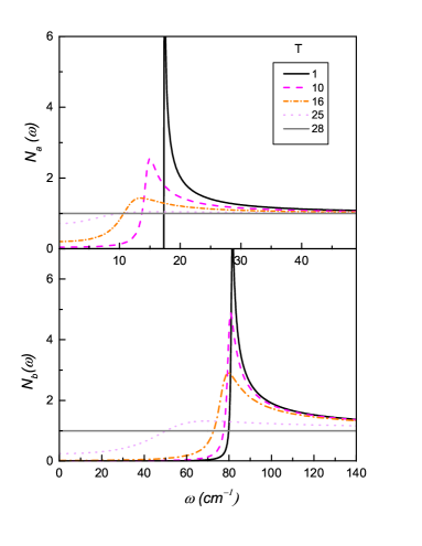
Figure 1: Density of states for the bands $a$ and $b$ calculated in strong coupling at various temperatures. The coupling constants are $\lambda_{aa}=0.5$, $\lambda_{ab}=0.2$, $\lambda_{ba}=0.1$, $\lambda_{bb}=3$. The superconducting critical temperature is $T_{c}=28\,cm^{-1}$. The DOS is normalized with respect to the normal state and is set equal to 1 for each band.

In the strong coupling approach, as opposed to the weak coupling limit, the gap functions are complex and frequency dependent $\tilde{\phi}_{\alpha}=\tilde{\phi}_{\alpha}(\omega)$. One of the consequences is the broadening of the quasiparticle peaks and appearing of the finite density of states $N_{\alpha}(\omega)=-\frac{1}{\pi}Img_{0\alpha}(\omega)$ at zero energy. This behavior is illustrated in Fig.1. At zero temperature, DOS in the strong coupling approach exhibits the coherence peak $N(\omega)\propto 1/\sqrt{\omega-\Delta}$ for $\omega\geq\Delta(\omega)$ and zero for $\omega<\Delta(\omega)$ quite similar to the weak coupling case. But at finite temperatures, DOS becomes finite for $\omega<\Delta(\omega)$ and the coherence peak is smeared out. This behavior is completely different from the weak coupling approximation. The reason is that the gap function $\Delta(\omega)$ in strong coupling approximation is a complex function. Accounting for the frequency dependence of the gap functions on the QPI is the key issue of the present work. At the same time, one has to point out that the DOS measurements are unable to distinguish between $s_{++}$ and $s_{\pm}$ order parameter symmetries (as is seen from Eq.3, DOS depends on $|\Delta(\omega,T)|$. A phase-sensitive QPI calculation is needed to bring out the contrast between the two types of pairing symmetries.

III Quasiparticle interference.

The STM measures the differential conductance; which, is proportional to the local single particle density of states $N(\mathbf{r},\omega)$:

$$\frac{dI}{dV}(\mathbf{r},\omega)\propto|M(\mathbf{r})|^{2}N(\mathbf{r},\omega),$$

where, $M(\mathbf{r})$ is the local tunnelling matrix element. The local density of states is related to the single particle retarded Green functions $G^{R}(\mathbf{r},\mathbf{r},\omega)$:

$$N(\mathbf{r},\omega)=-\frac{1}{\pi}\mbox{Im}Tr\left[\frac{1+\tau_{3}}{2}\hat{G}^{R}(\mathbf{r},\mathbf{r},\omega)\right]$$ (7)

Here, $Tr[..]$ is taken over both Nambu and band indices. Although the tunnelling matrix element may be important in the multiband case, sharpening the spectral weight contribution of some orbitals, the strong coupling does not affect the tunnelling matrix element. Since, we want to focus here on the effects of strong coupling the consideration is restricted by the impact of a single impurity on the local density of states. In the linear response approximation the perturbation of the density of states form due to an impurity with the point-like scattering $\displaystyle\hat{U}(\mathbf{r})=U_{\alpha\beta}\delta(\mathbf{r})\tau_{3}$ reads Dolgov2009 :

$$\delta N(\mathbf{r},\omega) = -\frac{1}{\pi}Im\sum_{\alpha,\beta}Tr\left[\frac{1+\tau_{3}}{2}\int dV^{\prime\prime}\hat{G}_{clean}^{\alpha}(\mathbf{r}-\mathbf{r}^{\prime\prime},\omega)\hat{U}_{\alpha\beta}(\mathbf{r}^{\prime\prime})\hat{G}_{clean}^{\beta}(\mathbf{r}^{\prime\prime}-\mathbf{r},\omega)\right]$$ (8)

for $\omega>0$. The negative values of $\omega$ can be obtained by substitution $\tau_{3}\to-\tau_{3}$. Since, in the response function, the bands are considered pairwise within the Born approximation; we will consider below the scattering between two bands, having in mind that one has to sum up the full response function afterwards. Considering Eq.(8) in the momentum space and keeping only the interband impurity scattering, which gives the leading contribution for the momentum $\mathbf{q}$ close to the interband vector $\mathbf{Q}$, we define the QPI response function $I(\mathbf{q},\omega)$ as:

$$\delta N(\mathbf{r},\omega)=U_{ab}\int\frac{d^{2}q}{(2\pi)^{2}}e^{i\mathbf{qr}}I(\mathbf{q},\omega)$$

The response function is given by the following expression:

$$I(\mathbf{q},\omega)=-\frac{1}{2\pi}\int\frac{d^{2}p}{(2\pi)^{2}}ImTr\left[\tau_{3}\hat{G}_{clean}^{a}(\mathbf{q+p},\omega)\tau_{3}\hat{G}_{clean}^{b}(\mathbf{p},\omega)\right]+(a\leftrightarrow b).$$ (9)

III.1 The model.

We apply the above formulation to develop the model for the general pnictide case as discussed below. In the low energy limit considered here, the spectrum near to the Fermi-level can be linearized:

$$\xi_{b}(\mathbf{p}+\mathbf{q})\approx\beta\xi_{a}(\mathbf{p})+\epsilon\cos 2\theta+\delta\mu.$$ (10)

Here, $sign\beta>0$ for impurity scattering between two electron or two hole bands, while $sign\beta<0$ for scattering between electron and hole bands. We assume constant density of states $\displaystyle N_{\alpha}=\int\delta(\xi_{\alpha,\mathbf{p}})d^{2}p/(2\pi)^{2}$ and $|\beta|=v_{b}/v_{a}$. Where, the $v_{a,b}$ are the Fermi velocities for the two bands. The parameter $\epsilon=\mathbf{k}_{Fy}\mathbf{v}_{b}-\mathbf{k}_{Fx}\mathbf{v}_{b}$ characterizes the ellipticity of the electron bands; where, $\mathbf{k}_{Fy}\,\text{and}\,\mathbf{k}_{Fx}$ are the electron band Fermi wave vectors. Here, $\theta$ is angle between the vector $\mathbf{p}$ and $\mathbf{q}$. We have $\epsilon=0$ for scattering between two hole bands; otherwise $\epsilon$ is finite. Finally, $\delta\mu$ accounts the relative energy shift of the Fermi-surfaces and is given by the relation $\delta\mu=(\mathbf{k}_{F}\mathbf{v}_{F})_{a}-(\mathbf{k}_{F}\mathbf{v}_{F})_{b}$.

III.2 Scattering at $q=Q$.

The direct integration over $\xi$ and the angle gives the following expression

$$I\!(\mathbf{q}=\mathbf{Q},\omega)\!=-\frac{\sqrt{N_{a}N_{b}}}{2}Im[K(\omega)F(\omega)],$$ (11)

where, the coherence factor $K(\omega)$ is

$$K(\omega)=\left[\frac{\tilde{\Delta}_{a}\tilde{\Delta}_{b}-\omega^{2}}{E_{a}E_{b}}\pm 1\right]$$ (12)

and

$$F \!\!\!(\omega)=\frac{1}{\sqrt{|\beta|^{-1}\epsilon^{2}-\!\left(\!\sqrt{|\beta|}\!Z_{a}\!E_{a}+\sqrt{|\beta|^{-1}}(\!Z_{b}\!E_{b}+\delta\mu)\right)^{2}}}\!$$ (13)

$$+ \!\!\frac{1}{\sqrt{|\beta|^{-1}\epsilon^{2}-\!\left(\!\sqrt{|\beta|}\!Z_{a}\!E_{a}+\sqrt{|\beta|^{-1}}(\!Z_{b}\!E_{b}-\delta\mu)\right)^{2}}}\!.$$

Here, $E_{\alpha}=\sqrt{\omega^{2}-\tilde{\Delta}_{\alpha}^{2}}$ is the quasiparticle energy spectrum. In the coherence factor $K(\omega)$ the sign ”+” corresponds to the scattering between two electron or two hole bands, while ”-” to the case of the scattering between electron and hole bands. One can immediately notice that the response function for intraband scattering at $q=0$ vanishes due to the coherence factor for all $\omega$. In our study, we have focussed completely on the inter-band interactions aspect of the phenomenon. This implies the choice of the ”-” sign in the relation for the coherence factor given by Eq.(12).

III.2.1 Zero ellipticity

The hole bands around $\Gamma$ point can be considered in a good approximations as circle ($\epsilon=0$). For simplicity, in discussing the two cases for the band ellipticity $\epsilon$, we shall assume the system to be in the weak coupling regime; and hence, take $\tilde{\Delta}_{\alpha/\beta}$ to be real and write it as $\Delta_{a/b}$ for the smaller (hole band) and larger (electron band) band gap energy, respectively. We start with perfectly matching hole bands ($\delta\mu=0$), having the gap functions $\Delta_{a}(\omega)>\Delta_{b}(\omega)$. The same ratio of the gap functions is used in the relation below. For the sake of simplicity, we put $\beta=1$ for further analysis. The function $I(\omega)$ diverges as $\displaystyle{\pm Re[1/\sqrt{\omega-\Delta_{b}}]}$ for $\omega>\Delta_{b}$ and as $1/\sqrt{|\omega-\Delta_{a}|}$ for $\omega$ close to $\Delta_{a}$. The sign in front of the first singularity depends on the symmetry of the order parameter. Sign ”$-$” corresponds to $s_{\pm}$ superconductivity, while ”$+$” for $s_{++}$ superconductivity. However, the sign in front of the second singularity does not depend on the superconducting order parameter symmetry. The mismatch of the bands creates non-zero $\delta\mu$, which, considerably changes the $\omega$-dependence of the response function. For very large values of $\delta\mu$, there is an additional dip at $\omega^{*}=\sqrt{(\Delta_{a}^{2}+\Delta_{b}^{2}+\delta\mu^{2})^{2}-4\Delta_{a}^{2}\Delta_{b}^{2}}/(2|\delta\mu|)$ at energy greater than $\Delta_{b}$. The divergence for energies near to $\Delta_{b}$ remains as $1/\sqrt{\omega-\Delta_{a}}$ for $\omega^{*}>\Delta_{a}$. The case for finite band ellipticity is considered below.

III.2.2 Finite ellipticity

For scattering between two electron bands, the essential role is played by the ellipticity of the electron bands i.e. $\epsilon$. Here, we have distinct cases: a) $|\epsilon|+|\delta\mu|<\Delta_{b}$, b) $|\epsilon|+|\delta\mu|>\Delta_{b}$ and $||\epsilon|-|\delta\mu||<\Delta_{a}$, c) $||\epsilon|-|\delta\mu||>\Delta_{a}$. For the case a) one finds the behaviour similar to the scattering between two hole bands i.e. the appearance of a dip. In the case b) in addition to $1/\sqrt{\omega-\Delta_{b}}$ and $1/\sqrt{\Delta_{a}-\omega}$ a new divergence of $1/\sqrt{\omega-\omega_{1}}$ appears at $\omega_{1}=\sqrt{(\Delta_{a}^{2}+\Delta_{b}^{2}+(\delta\mu+|\epsilon|)^{2})^{2}-4\Delta_{a}^{2}\Delta_{b}^{2}}/(2(|\delta\mu|+|\epsilon|))$. In the case c) one additional divergence $1/\sqrt{\omega-\omega_{2}}$ occurs at $\omega_{2}=\sqrt{(\Delta_{a}^{2}+\Delta_{b}^{2}+(\delta\mu-|\epsilon|)^{2})^{2}-4\Delta_{a}^{2}\Delta_{b}^{2}}/(2||\delta\mu|-|\epsilon||)$.

III.3 Scattering at $q=Q+\tilde{q}$

Now, we consider the quasiparticle interference due to interband scattering at the vector $\mathbf{\tilde{q}}=\mathbf{q}-\mathbf{Q}$. For small $\tilde{q}$ one can use the approximation $\xi_{b}(\mathbf{p}+\mathbf{q})\approx\beta\xi_{a}(\mathbf{p})+\epsilon\cos 2\theta+v_{b}\tilde{q}\cos(\theta-\phi)+\delta\mu$, where $\phi$ is the angle between the vector $\tilde{\mathbf{q}}$ and $\mathbf{Q}$. The F-function in Eq.(11) has the form:

$$F(\omega,\phi)=\left\langle\frac{\!\sqrt{|\beta|}Z_{a}E_{a}+\sqrt{|\beta|^{-1}}Z_{b}E_{b}}{(\!\sqrt{|\beta|}Z_{a}E_{a}\!+\!\sqrt{|\beta|^{-1}}Z_{b}E_{b})^{2}\!+|\beta|^{-1}\left(\epsilon\cos(2\theta)\!+\!v_{b}\tilde{q}\cos(\theta-\phi)\!+\!\delta\mu\right)^{2}}\right\rangle_{\!\!\theta\,},$$ (14)

where $\langle...\rangle_{\theta}$ is the averaging over the angle. The integration over the angle can be easily performed in two limits of $\epsilon\gg\mathbf{v}_{b}\mathbf{\tilde{q}}$ (setting $\mathbf{v}_{b}\mathbf{\tilde{q}}=0$) and $\epsilon\ll\mathbf{v}_{b}\mathbf{\tilde{q}}$ (setting $\epsilon=0$). In the second limit we recover expression similar to Eq.(13) with substitution $\epsilon\to\mathbf{v}_{b}\mathbf{\tilde{q}}$.

IV Numerical Analysis and Results

In the following, we will apply the above general formulation to Fe-BS, using the electron-boson spectral function, successfully used by Popovich et. al.Popo2010 for the thermal studies and by Charnukha et. al.Charnukha2010 for optical conductivities for the description of BaKFeAs at optimal doping. According to Charnukha2010 , the original four-band model for $Ba_{1-x}K_{x}Fe_{2}As_{2}$ can be reduced to an effective two-band model, where the first band is formed by the inner hole pocket with the gap $\Delta_{a}$, while the second band with the gap $\Delta_{b}>\Delta_{a}$ consists from combination of two electron pockets and outer hole pocket. Within this two-band model we will calculate the response $I(\mathbf{q},\omega)$ at $\mathbf{q}$ values around the nesting vector $\mathbf{Q}=(\pi,\pi)$.

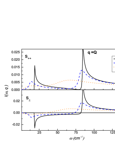
Figure 2: The response function I($\omega$) for the $s_{++}\,\text{and}\,s_{\pm}$ case with the strong coupling $\lambda$-matrix defined as ($\lambda_{aa}$=3, $\lambda_{ab}$=${\pm}$0.2, $\lambda_{ba}$=${\pm}$0.1, $\lambda_{bb}$=0.5) and $T_{c}$ =28 $cm^{-1}$.

The model is studied in the beginning with $\epsilon=\delta\mu$ =0 (non-FeBS case), and later in the paper, we would consider finite values of $\delta\mu$ and $\epsilon$, as is the case with pnictides. Hence, the model has broader implications to other high $T_{c}$ superconductors. In this case, we have only two characteristic energy values, namely the energies of the gaps $\Delta_{a}$ and $\Delta_{b}$. Our purpose is to identify certain peculiarities of the QPI response for the $s_{++}$ and $s_{\pm}$ pairing symmetries. The resulting real-valued energy gaps in $N_{\alpha}(\omega)$, as discussed in Fig.1, are $\Delta_{a}$ = 17 $cm^{-1}$, while $\Delta_{b}$ = 83 $cm^{-1}$ at T = 0, which gives a gap ratio $\Delta_{b}/\Delta_{a}$ = 4.82.

In Fig. 2, we discuss the temperature evolution of the response function for $s_{++}$ and $s_{\pm}$ symmetry. First, at temperature T =1, the QPI response vanishes for $\omega<\Delta_{a}$ for both $s_{++}$ and $s_{\pm}$ order parameters; since, there is no excitation at the energy below $\Delta_{a}$. In the whole temperature range, the response function for $s_{++}$ superconductivity is positive for all values of $\omega$; while in the $s_{\pm}$ case, for energies around the smaller gap, it is negative. As the temperature increases, the response related to the $s_{\pm}$ symmetry turns positive at much lower energies, while for $s_{++}$ case, the response peak shows a gradual shift towards the energy interval between the two band gaps. To sum up, the main feature that help us to distinguish between the response behaviour for the $s_{++}$ and $s_{\pm}$ symmetry cases is the robustness of the sign of the peaks near the small band gap $\Delta_{a}$ over a broad range of $T<T_{c}$.

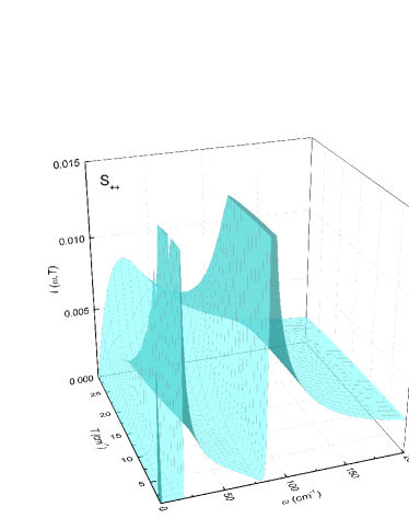
(a) $s_{++}$ symmetry

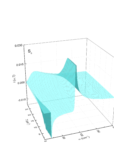
(b) $s_{\pm}$ symmetry

Figure 3: 3D plot of the response function vs temperature at fixed energy $\omega$ for $s_{++}$ (upper) and $s_{\pm}$ (lower) cases, respectively. The coupling parameters are the same as used above and the transition temperature, $T_{c}$=28 $cm^{-1}$.

The Fig. 3 represents the 3D plot depicting the variation of $I(\omega)$ simultaneously with temperature T and energy $\omega$ for the case of perfect nesting i.e. $\mathbf{q}=\mathbf{Q}$. For $s_{++}$ symmetry, at low temperatures and $\omega\leq\Delta_{a}$, we consider the slice in the region $0<T<10$ that shows a small sharp peak which dips smoothly as the temperature rises. Moving towards high energies and at low temperatures,the peak around the second band gap energy is very strong and decays much slower with rising temperature and energy than compared to the first peak. While in the $s_{\pm}$ case, we see the difference for the first band peak as the response at low temperature and low energy is inverted (at $\omega\leq$ 20) and has large magnitude. This is the main feature that reflects throughout our analysis. The peaks around the first band gap energy are a robust indication of the difference between the two symmetry cases viz. $s_{++}$ and $s_{\pm}$.

In the region of sub-gap energies and low temperatures, the $s_{++}$ response shows a negative gradient while the $s_{\pm}$ curve is almost flat and is negative; and for the same energies at high temperatures, the behaviour is similar for both the symmetries and hence it is indistinguishable in this region. Beyond that, the graph shows a monotonically decreasing trend for both $s_{++}$ and $s_{\pm}$ response function and does not provide any interesting distinguishable feature apart from the greater signal strength for $s_{++}$ curve than the latter. As we move to the higher temperatures, a bump in the response function arises, which is appreciably diffused and broadened as compared to the ones at low temperatures. This behaviour of response function is same, in both $s_{++}$ and $s_{\pm}$ case for $T>$25 as stated for the Fig. 2.

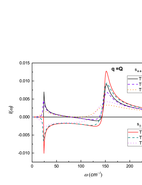
Figure 4: The QPI response function for the $s_{++}$ and $s_{\pm}$ case at very strong couplings $\tilde{\lambda}$ i.e. $\lambda_{aa}$=1,$\lambda_{bb}$=6,$\lambda_{ab}$=0.4, $\lambda_{ba}$=0.2 with the transition temperature $T_{c}$ =46 $cm^{-1}$.

For Fig. 4, we have I($\omega$) vs energy $\omega$ plotted at various temperatures with very strong coupling parameters $\tilde{\lambda}$ and a raised transition temperature i.e. $T_{c}$ = 46. In the subgap region, for the s₊₊ case, we identify a peculiar behaviour of the response function (compare Fig. 2) as it goes to negative values and peaks just like the response for $s_{\pm}$ case. In summary, for the energies near the second band gap, the behaviour of response function for both the symmetry cases is indistinguishable apart from their relative strengths. However, we again observe that the response peaks near the smaller gap are a defining and distinguishing feature even for a very strong coupling case.

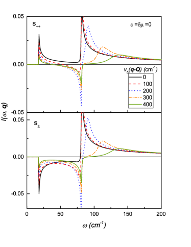
Figure 5: The 2D plot of the QPI response function I($\omega$) vs $\omega$ and the momentum $\mathbf{q}$ for the strong coupling case with $\epsilon=\delta\mu$ = 0 at temperature T = 1. The values of the coupling constants are $\lambda_{aa}=0.5$, $\lambda_{ab}=0.2$, $\lambda_{ba}=0.1$, $\lambda_{bb}=3$.

In the following, we present the study of the response function behaviour with respect to the changes in parameters such as the ellipticity $\epsilon$ of the electron-like bands, the shifted Fermi energy $\delta\mu$ between the hole-like and the electron-like bands and the experimentally tunable electron momentum parameter $v_{b}\tilde{q}$; which, points in the radial direction to the electron band Fermi surface. Here, $\mathbf{\tilde{q}}$ is tuned in order to obtain the correct matching condition for the shifted Fermi energy surface, as discussed later, and to study the response behaviour closer to the region of Fermi surface instability, as followed from Eq.(14).

In the Figs. 5 and 6, we plot in 2D and 3D, the behavior of $\mathbf{q}$-resolved response function for both the symmetry cases, with variation in the electron-like quasiparticle momentum $\mathbf{\tilde{q}}$ using Eq.(14) and setting the ellipticity and surface energy to zero. We also assume that the momentum vector $\tilde{\mathbf{q}}$ is directed along ${\mathbf{Q}}$ and hence, the angle $\phi$ =0. The finite value of $\mathbf{\tilde{q}}$ relates to the fact that we are probing the Fermi surface of the electron-like band pocket. We have $||\epsilon|-|\delta\mu||<\Delta_{a}$ satisfied in this case. For the peak near larger band gap energy, the amplitude and the sign of the peak are robust and distinguishing features.

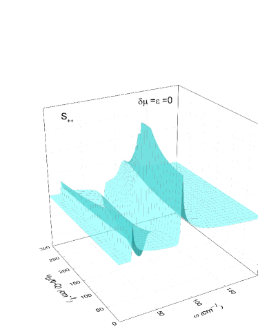
(a) $s_{++}$ symmetry

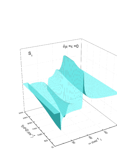
(b) $s_{\pm}$ symmetry

Figure 6: The 3D plot of the QPI response function I($\omega$) vs $\omega$ and momentum $\mathbf{q}$ with the zero ellipticity $\epsilon$=0 and zero shifted Fermi surface energy $\delta\mu$=0 for the strong coupling case at temperature T = 1. The values of the coupling constants are $\lambda_{aa}=0.5$, $\lambda_{ab}=0.2$, $\lambda_{ba}=0.1$, $\lambda_{bb}=3$..

We see that the energy dependence of the response function at finite $\mathbf{\tilde{q}}$ shows three peaks. Two of these are momentum independent and correspond to the gaps in the bands $\Delta_{a}$ and $\Delta_{b}$, while the third peaks has a strong $\mathbf{\tilde{q}}$ dependence. The strong difference between $s_{++}$ and $s_{\pm}$ symmetries we see only for the first peak at he energy of the small gap. For the $s_{\pm}$ order parameter the response function at $\omega=\Delta_{a}$ is negative, while for $s_{++}$ it is positive. It leads to the conclusion that for determining the symmetry of the order parameter, one has to consider the response function at momenta close to the nesting vector $\mathbf{Q}$, and find the momentum independent peaks. The smallest of these peak will determine the symmetry of the order parameter.

The QPI response at energies close to the second gap $\Delta_{b}$ is shown in Fig.2 for $\mathbf{\tilde{q}}$ i.e. ($\mathbf{q}-\mathbf{Q}$) has opposite sign compared to the results presented by Hirschfeld et. alHirschfeld15 , using a similar model in the weak-coupling regime. The results presented in Figs. 5 and 6 clearly demonstrate that with the increase of $\tilde{\mathbf{q}}$, the sign of the second peak reverses. In this respect, our results do not contradict to those of Hirschfeld15 , $\mathbf{q}$-integrated response function was presented to be dominated by large $\mathbf{q}$ values. Moreover, our $\mathbf{q}$-resolved results provide more information about the QPI response behaviour. In particular, for non-zero ellipticity $\epsilon$ or the non-zero chemical potential shift $\delta\mu$, we have obtained additional mode at energies above $\Delta_{b}$ as shown in Figs. (5-11).

Hence, we again argue that the peak near the first band gap energy i.e. $\omega\approx\Delta_{a}(\omega)$ is the only strong distinguishing feature for the phase sensitive experiments for the gap symmetry measurements.

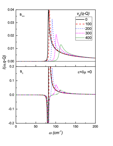
Figure 7: The 2D plot of the QPI response function I($\omega$) vs $\omega$ and momentum $\mathbf{q}$ for the strong coupling case, with $\Delta_{a}=\Delta_{b}$, and $\epsilon=\delta\mu$ = 0 at temperature T = 1; with the coupling constants given as $\lambda_{aa}=0.5$, $\lambda_{ab}=0.2$, $\lambda_{ba}=0.1$, $\lambda_{bb}=3$.

So far, we explored the region around the nesting vector $\mathbf{Q}=(\pi,\pi)$ with scattering between the smaller/inner hole-like band to the outer/larger averaged electron-like band. Now, we focus on the scattering of the quasiparticles from electron-like band to the outer hole-like band with larger gap value i.e. $\tilde{\Delta}_{a2}(\omega)\rightarrow\tilde{\Delta}_{b1/b2}(\omega)$. In Fig. 7, we plot the response function for various values of the electron-like quasiparticle momentum $\mathbf{\tilde{q}}$ over full spectrum of energy $\omega$ with equal band gap functions. For this, we modify Eq.(12) by the substitution of the full gap function $\tilde{\Delta}_{a}(\omega)\rightarrow\tilde{\Delta}_{b}(\omega)$ i.e. we replace the inner hole band gap function by the outer/larger hole band gap function, such that, we also replace all the corresponding renormalization functions i.e. $Z_{a}\rightarrow Z_{b}$ and the related density of states.

For $s_{++}$ symmetry, we find that the response function for the energies $\omega<\Delta_{b}$ is zero over a large range and becomes non-zero only at $\omega=75\,cm^{-1}$ and remains positive afterwards. This is in contrast to the behaviour of the response function given in Fig.5, for the same symmetry. Where, the function goes through the zero towards the negative peak situated near the larger gap energy i.e. $\Delta_{b}$. Only for $\mathbf{\tilde{q}}=0$, we have a response function that stays positive over the full energy range. At energies $\omega\geq\Delta_{b}$, we observe that the response function peaks are shifted towards higher energies with increase in $\mathbf{\tilde{q}}$ in both the figures. However, in Fig.7, for the $s_{++}$ case, there are only single positive peaks, i.e. only single mode, for all the $\mathbf{\tilde{q}}$.

In the $s_{\pm}$ case, as depicted in Fig. 7, the response function amplitude has a very large value, in fact an order of magnitude larger, than the $s_{++}$ case in the same figure and also in comparison to the response amplitudes in Fig.5. for both the $s_{++}$ and $s_{\pm}$ symmetry case. The reason for such a behaviour is the contribution of the divergent term $1/(\Delta_{b}-\omega)$ in the coherence factor $K(\omega)$ for the $s_{\pm}$ case, instead of a constant scalar multiple for the $s_{++}$ case (see Eq.(13)). In the region $\omega\approx\Delta_{b}$, there is a large negative peak of the response function. At $\omega>\Delta_{b}$ both the graphs in the upper and lower panel of Fig.7 are qualitatively similar for the increasing value of $\mathbf{\tilde{q}}$, along with the presence of an additional mode, which is shifted towards higher values of $\omega$, in all the cases without exception.

Although, a difference is present between both the symmetries at $\omega\approx\Delta_{b}$ for this scattering; it only exists within a very narrow energy range. Hence, we shall confine the study to the previous case of the scattering of quasiparticles between the smaller/inner hole-like band the gap-averaged electron-like bands to study QPI. In the following, we emphasize that this robustness of the QPI response peak, with respect to various parameters, provides an ideal tool to probe the order parameter phase symmetry.

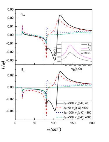
Figure 8: The 2D plot of the QPI response function I($\omega$) vs $\omega$, momentum $\mathbf{q}$ and the shifted Fermi surface energy $\delta\mu$ for the strong coupling case at temperature T = 1. In the inset, the dependence of $|I(\mathbf{q-Q})|$ is shown at fixed energy close to the smaller gap i.e. $\omega\approx$ 18 $cm^{-1}$. The values of the coupling constants are $\lambda_{aa}=0.5$, $\lambda_{ab}=0.2$, $\lambda_{ba}=0.1$, $\lambda_{bb}=3$.

In Fig. 8, the graph depicts the behaviour of the QPI response function for very large shifted Fermi surface energy i.e. $\delta\mu$=300 and the comparison with the case of zero $\delta\mu$ and non-zero value $\mathbf{v}_{b}\mathbf{\tilde{q}}$ for both the symmetry cases. The behaviour of $\mathbf{v}_{b}\mathbf{\tilde{q}}$ is shown by dashed curves as the momentum vector $\mathbf{\tilde{q}}$ varies from small to large values and connects the two order parameters on the Fermi surfaces when its of the order $(\pi)$. The black curve shows the behaviour of the response function for zero momentum and large shifted Fermi surface energy. The red dashed curve for zero $\delta\mu$ and large $\mathbf{v}_{b}\mathbf{\tilde{q}}$, shows the difference in the two cases with a shifting of the peak that arises for $\omega>\Delta_{b}$.

For the equal values of both the parameters, the behaviour is depicted by the blue dotted curve; where, the inverted peaks near the first and second band gap energies are almost equal in magnitude. Finally, the green curve shows the case for very large electron like quasiparticle momentum in comparison to the shifted Fermi surface energy and shifted peak is shown to be highly dispersed. The value of $\omega^{*}$ calculated through relation $\omega^{*}=\sqrt{(\Delta_{a}^{2}+\Delta_{b}^{2}+\delta\mu^{2})^{2}-4\Delta_{a}^{2}\Delta_{b}^{2}}/(2|\delta\mu|)$, for the case when $\delta\mu>\Delta_{b}$ is 162.03 $cm^{-1}$.

As stated previously, the most robust feature is the peak of the response function around the first band gap energy, which does not change the sign reversing behaviour with the change in parameters viz. $\delta\mu$, $\epsilon$ or $\mathbf{\tilde{q}}$ in the Eq.(14). Hence, this characteristic of the QPI response function presents itself as a very useful feature for the probe of order parameter symmetry between the $s_{++}$ and $s_{\pm}$ case, via the c-axis measurements from the FT-STM studies.

The inset in the upper panel of Fig. 8, depicts the strong dependence of the magnitude of the peak on the parameter $\mathbf{\tilde{q}}$. For the perfect nesting case, i.e. $\mathbf{q}=\mathbf{Q}$, we observe the maximum in response function magnitude. For a fixed $\delta\mu$ and for the energy chosen to be near $\Delta_{a}$, we have the experimentally tunable parameter $\mathbf{\tilde{q}}$ start at zero and scan over larger values. The peaks of $|I(\mathbf{\tilde{q}})|$ in both the symmetry cases emerge for some optimal value of the momentum i.e. when $\mathbf{\tilde{q}}$ becomes of the order $\delta\mu$ (in accordance with Eq.(14)). At small values of $\mathbf{\tilde{q}}$, this magnitude of the peaks is quite small; and hence, to observe this experimentally, we need to find the match between the large value of $\mathbf{\tilde{q}}$ and $\delta\mu$ to sample such behaviour correctly.

V Summary & Conclusion

We have analysed the problem of the identification of the order parameter symmetry for the Fe-based superconductors via the QPI measurements. For this purpose, we have developed a theory of the quasiparticle interference in multiband superconductors based on strong-coupling Eliashberg approach. In particular case of a two-band system, we consider two possible pairing symmetries the $s_{\pm}$ state, when the sign of the order parameters changes between the hole and the electron bands and the more conventional $s_{++}$ state.

The obtained results confirm the concept that the QPI is phase-sensitive technique and may help to determine pairing symmetry in Fe-based superconductors; and in general, could be applicable to other multiband superconductors. We calculate energy, temperature and momentum dependencies of the QPI response and point out qualitative differences between the response in the $s_{\pm}$ and $s_{++}$ cases. Application of the Eliashberg approach allows to take into account self-consistent retardation effects due to strong coupling and to properly describe temperature dependence of the QPI response function at various energies. Further, we have analyzed various regimes of the Fermi surface anisotropy by taking into account the influence of Fermi surface ellipticity.

We argued from the analysis that, in general, for $\mathbf{q}\approx\mathbf{Q}$, there are three singularities of the response function. Two of these are momentum independent (weak momentum dependence) $\omega\approx\Delta_{a,b}(\omega)$ and the one having a strong momentum dependence. Only the momentum independent (weak momentum dependence) peak, corresponding to the lowest gap value $\Delta_{a}$, may serve as a universal probe for the gap symmetry in the multiband superconductors. We emphasize that our analysis presents a convincing case in favour of the QPI measurements as a phase sensitive test of the gap symmetry for the FeBS. This conclusion is based on the robustness of the response function peak near the smaller gap energy and is independent of the exact nature or shape of the energy bands.

VI Acknowledgements

We acknowledge useful discussions with P. Hirschfeld, I.I. Mazin, D. Morr and Y. Tanaka. This work was financially supported by the Foundation for Fundamental Research on Matter (FOM), associated with the Netherlands Organization for Scientific Research (NWO), by Russian Science Foundation, Project No. 15-12-30030, and by Ministry of Education and Science of the Russian Federation, grant 14.Y26.31.0007. DE acknowledges DFG financial support through the grant GR 3330/4-1 and financial support of VW-foundation through the grant “Synthesis, theoretical examination and experimental investigation of emergent iron-based superconductors”.

VII Appendix

Here, we show the 2D and 3D graphs for the response function variation with shifted Fermi surface energy $\delta\mu$ versus the energy $\omega$ and with the electronic band ellipticity, $\epsilon$ = 0, for both the $s_{++}$ and $s_{\pm}$ cases, as discussed in the main text under sec. III(B).

First, in Fig. 9, the trend for the response function at zero ellipticity is presented. The response curve near the second band gap energy has a sharp small negative peak and a broadened secondary peak as the $\delta\mu$ values increase. The second peak shifts away from $\Delta_{b}$ with larger values of shifted Fermi energy between the electron-like and hole-like pockets and for very large $\delta\mu$ the two lower peaks become relatively similar in strength. The positive peak around the same energy interval also shows a shift towards $\omega>\Delta_{b}$ and flattens out at very high $\delta\mu$ value. Here, again we observe that the peaks around the smaller band gap is a robust feature with respect to the variation in the parameters.

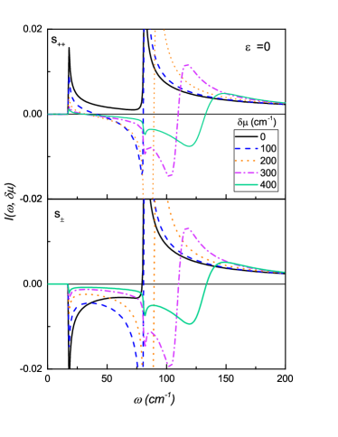
Figure 9: The 2D plot of the QPI response function I($\omega$) vs $\omega$ and the shifted Fermi surface energy $\delta\mu$ for the strong coupling case at temperature T = 1 at ellipticity $\epsilon$ and the momentum $\tilde{q}$ =0. The values of the coupling constants are $\lambda_{aa}=0.5$, $\lambda_{ab}=0.2$, $\lambda_{ba}=0.1$, $\lambda_{bb}=3$.

The 3D graph in Fig. 10, shows the change in response function as we move from $\omega<\Delta_{a}$ to the region $\omega>\Delta_{b}$. The response function gets the inverted peak near the second band gap energy in both the cases and there is a secondary dip that shifts towards higher energy with increasing shifted Fermi surface energy. The shift of the second peak at $\omega>\Delta_{b}$ is observed. There is almost similar amplitude of the QPI response in both the cases with the strong coupling around the region $\omega$ = $\Delta_{a}$ for $\epsilon$ =0 case as compared to Fig. 2. For higher energies and larger chemical potential, apart from strong peaks, we have no other distinguishing feature for both the cases except for the QPI peak around the smaller band gap, $\Delta_{a}$.

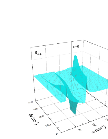
(a) $s_{++}$ symmetry

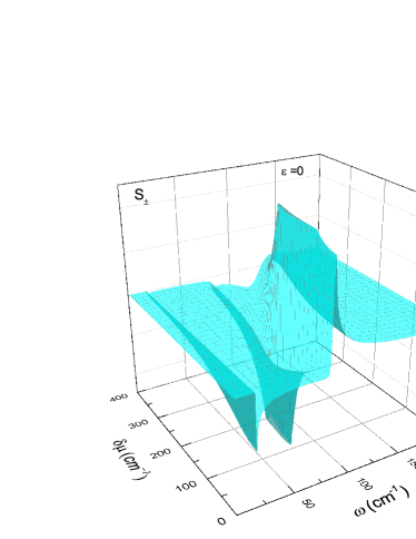
(b) $s_{\pm}$ symmetry

Figure 10: The 3D plot of the QPI response function I($\omega,\delta\mu$) vs $\omega$ and the non-zero Fermi surface energy $\delta\mu$ at zero ellipticity for the strong coupling case at temperature T = 1 for $s_{++}$ and $s_{\pm}$. There is a large amplitude for the response function in the region $\delta\mu$=[100,200] for the latter case. The values of the coupling constants are $\lambda_{aa}=0.5$, $\lambda_{ab}=0.2$, $\lambda_{ba}=0.1$, $\lambda_{bb}=3$.

The effect of the relative shift of the Fermi surface energy to a non-zero value shows that there is a rather strong suppression of the second response peak in $s_{++}$ case as compared to the $s_{\pm}$ in the region $\omega\approx\Delta_{b}$ as compared to the finite ellipticity case discussed below.

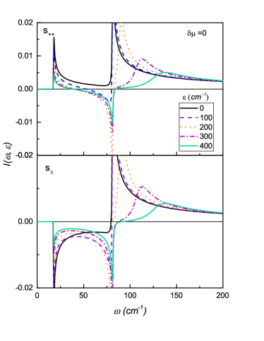
Figure 11: The 2D plot of the QPI response function I($\omega$) vs $\omega$ and the ellipticity $\epsilon$ for the strong coupling case with value of shifted Fermi surface energy $\delta\mu$ and the momentum $\tilde{q}$ =0, at temperature T = 1. The values of the coupling constants are $\lambda_{aa}=0.5$, $\lambda_{ab}=0.2$, $\lambda_{ba}=0.1$, $\lambda_{bb}=3$.

In Figs. 11 and 12, we present the change of the response function with variation in the band ellipticity $\epsilon$ as in Eq.(13) and setting the shift in Fermi surface energy $\delta\mu$ = 0 with 2D and 3D graphs. The larger ellipticity values lead to the inversion of the peak around second band gap, which reaches its maximum value around $\epsilon$ =200 and thereafter the overall amplitude drops, with the positive peak dampening strongly and shifting towards higher $\omega$ values. The peaks near the first band gap energy are unaltered by the change of the ellipticity and hence present a strong case for the probing of the gap symmetry based on QPI experiments.

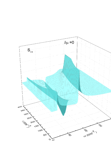
(a) $s_{++}$ symmetry

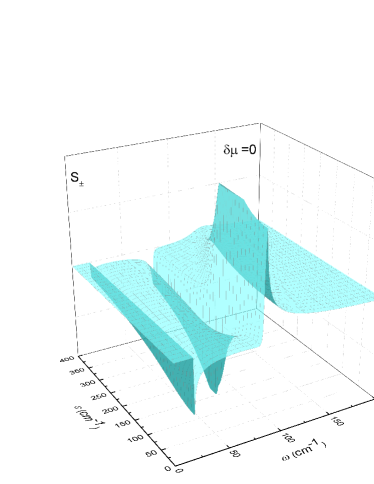
(b) $s_{\pm}$ symmetry

Figure 12: The 3D plot of the QPI response function I($\omega$) vs $\omega$ and the ellipticity $\epsilon$ for the strong coupling case with value of shifted Fermi surface energy $\delta\mu$ and the momentum $\tilde{q}$ =0, at temperature T = 1. The values of the coupling constants are $\lambda_{aa}=0.5$, $\lambda_{ab}=0.2$, $\lambda_{ba}=0.1$, $\lambda_{bb}=3$.

Additionally, for the energies close to the second band gap energy and with a large $\epsilon$, the response function is negatively peaked for both the cases and has a stronger peak around $\epsilon$ =200 with a very strongly damping for very high ellipticity values. In both the cases, we observe the shifting and high suppression of the positive peak towards energies $\omega>\Delta_{b}$ and the negative response peak just falls off very slowly without the shift. This gains confirms our assertion that the smaller band gap peak is a promising feature that could be used as a universal tool for the pairing symmetry measurements.

References

- (1) Y. Kamihara, T. Watanabe, M. Hirano, H. Hosono, J. Am. Chem. Soc., 130 , 3296, (2008).
- (2) G.R. Stewart, Rev. Mod. Phys. 83, 1589, (2011).
- (3) J. Paglione and R.L. Greene, Nat. Phys. 6, 645, (2010).
- (4) D.C. Johnston, Adv. Phys. 59, 803, (2010).
- (5) H. Hosono, K. Kuroki, Physica C 514 399, (2015).
- (6) I. I. Mazin, O. K. Andersen, O. Jepsen, O.V. Dolgov, J. Kortus, A. A. Golubov, A. B. Kuzmenko, and D. van der Marel, Phys. Rev. Lett. 89, 107002, (2002).
- (7) C. de la Cruz, Q. Huang, J. W. Lynn, Jiying Li, W. Ratcliff , J. L. Zarestky, H. A. Mook, G. F. Chen, J. L. Luo, N. L. Wang & P. Dai, Nature, 453, 899, (2008).
- (8) T. Hidenori, Nature Materials 8, 251, (2009).
- (9) D. K. Pratt, W. Tian, A. Kreyssig, J. L. Zarestky, S. Nandi, N. Ni, S. L. Bud’ko, P. C. Canfield, A. I. Goldman & R. J. McQueeney, Phys. Rev. Lett. 103, 087001, (2009).
- (10) P. J. Hirschfeld, C. R. Physique 17, 197-231, (2016).
- (11) J-Feng Ge, Zhi-Long Liu, C. Liu, C-Lei Gao, D. Qian, Qi-Kun Xue, Y. Liu J-Feng Jia, Nature Materials 14, 285-289, (2015).
- (12) D. J. Singh & M. H. Du, Phys. Rev. Lett., 100, 237003, (2008).
- (13) Y. Yamakawa & H. Kontani, Phys. Rev. B 92, 045124, (2015).
- (14) I. I. Mazin, D. J. Singh , M. D. Johannes & M.H. Du , Phys. Rev. Lett.101, 057003, (2008).
- (15) McElroy et. al, Nature 422, 592 (2003)
- (16) P.J. Hirschfeld, M.M. Korshunov, & I.I. Mazin, Rep. Prog. Phys. 74,124508, (2011).
- (17) Mazin, I. I., Nature 464, 183 (2010).
- (18) A. V. Chubukov, D. V. Efremov & I. Eremin, Phys. Rev. B, American Physical Society, 78, 134512 (2008).
- (19) T. Hanaguri, S. Niitaka, K. Kuroki, & H. Takagi, Science, 328, 474 (2010).
- (20) A. A. Kordyuk, Low Temperature Physics, 38, 888,(2012).
- (21) K. Kuroki, S. Onari, R. Arita, H. Usui, Y. Tanaka, H. Kontani & H.Aoki, Phys. Rev. Lett. 101,087004, (2008).
- (22) P. Werner, M. Casula, T. Miyake, F. Aryasetiawan, A. J. Millis & S.Biermann Nature Physics 8, 331â(2012).
- (23) X. Chen, P. Dai, D. Feng, T. Xiang & F. C. Zhang, National Science Review, 1, 371 (2014).
- (24) P. Monthoux & G. G. Lonzarich, Phys. Rev. B, 63, 054529 (2001).
- (25) P. J. Hirschfeld, M. M. Korshunov & I. I. Mazin, Reports on Progress in Physics, 74, 124508 (2011).
- (26) L. Boeri, O. V. Dolgov, and A. A. Golubov, Phys. Rev. Lett. 101, 026403 (2008).
- (27) D.V. Efremov, M. M. Korshunov, O.V. Dolgov, A. A. Golubov, & P. J. Hirschfeld, Phys. Rev. B 84, 180512 (2011).
- (28) M. M. Korshunov, D.V. Efremov, A. A. Golubov, and O.V. Dolgov, Phys. Rev. B 90, 134517 (2014).
- (29) D.V. Efremov, A. A. Golubov & O. V. Dolgov, New Journal of Physics, 15,013002 (2013).
- (30) M. B. Schilling, A. Baumgartner, B. Gorshunov, E. S. Zhukova, V. A. Dravin, K.V. Mitsen, D.V. Efremov, O.V. Dolgov, K. Iida, M. Dressel, and S. Zapf, Phys. Rev. B 93, 174515 (2016).
- (31) J. P. Reid, M. A. Tanatar, A. Juneau-Fecteau, R. T. Gorton, S. R. de Cortret, N. Doiron-Leyraud, T. Saito, H. Fukuzawa, Y. Kohoni, K. Kihour, C. H. Lee, A. Iyo, H. Eisaki, R. Prozorov, and L. Taillefer, Phys. Rev. Lett. 109, 087001 (2012).
- (32) M. Abdel-Hafiez, V. Grinenko, S. Aswartham, I. Morozov, M. Roslova, O. Vakaliuk, S. Johnston, D.V. Efremov, J. van den Brink, H. Rosner, M. Kumar, C. Hess, S. Wurmehl, A. U. B. Wolter, B. Buechner, E. L. Green, J.Wosnitza, P. Vogt, A. Reifenberger, C. Enss, M. Hempel, R. Klingeler, and S. L. Drechsler, Phys. Rev. B 87 180507 (2013).
- (33) V. Grinenko, D.V. Efremov, S. L. Drechsler, S. Aswartham, D. Gruner, M. Roslova, I. Morozov, K. Nenkov, S. Wurmehl, A. U. B. Wolter, B. Holzapfel, and B. Buechner, Phys. Rev. B 89,060504 (2014).
- (34) V. Grinenko, W. Schottenhamel, A. U. B. Wolter, D.V. Efremov, S. L. Drechsler, S. Aswartham, M. Kumar, S. Wurmehl, M. Roslova, I.V. Morozov, B. Holzapfel, B. Buechner, E. Ahrens, S. I. Troyanov, S. Koehler, E. Gati, S. Knoener, N. H. Hoang, M. Lang, F. Ricci, and G. Profeta, Phys. Rev. B 90, 094511 (2014).
- (35) Q.Wang, J. T. Park, F. Y., Y. Shen, Y. Hao, Y. Pan, J. Lynn, A. Ivanov, S. Chi, M. Matsuda, H. Cao, R. J. Birgenau, D.V. Efremov, and J. Zhao, Phys. Rev. Lett. 116, 197004 (2016).
- (36) A. A. Golubov & I. I. Mazin, Applied Physics Letters, 102, (2013).
- (37) D. Parker & I. I. Mazin, Phys. Rev. Lett. 102, 227007, (2009).
- (38) A. V. Burmistrova, I. A. Devyatov, A. A. Golubov, K. Yada, Y. Tanaka, M. Tortello, R. S. Gonnelli, V. A. Stepanov, X. Ding, H. H. Wen, & L. H. Greene, Phys. Rev. B 91, 214501, (2015).
- (39) A. A. Golubov, A. Brinkman, Yukio Tanaka, I. I. Mazin, & O. V. Dolgov, Phys. Rev. Lett. 103, 077003, (2009).
- (40) M.F. Crommie et. al, Nature, 363, 524- 527 (1993).
- (41) K. Kanisawa, M. J. Butcher, H. Yamaguchi & Y. Hirayama, Phys. Rev. Lett., 86, 3384 (2001).
- (42) J. E. Hoffman, K. McElroy, D.H. Lee, K. M. Lang, H. Eisaki, S. Uchida, J. C. Davis, Science, 297, 1148 ( 2002).
- (43) C. Howald, H. Eisaki, N. Kaneko, M. Greven, and A. Kapitulnik, Phys. Rev. B, 67, 014533 (2003).
- (44) T. Hanaguri, Y. Kohsaka, J. C. Davis, C. Lupien, I. Yamada, M. Azuma, M. Takano, K. Ohishi, M. Ono & H. Takagi, Nature Physics , 3, 865 (2007).
- (45) L. Capriotti, D. J. Scalapino & R. D. Sedgewick, Phys. Rev. B, 68,014508 (2003).
- (46) M. Maltseva and P. Coleman, Phys. Rev. B 80, 144514 (2009).
- (47) S. Sykora and P. Coleman, Phys. Rev. B 84, 054501 (2011).
- (48) P.J. Hirschfeld, D. Altenfeld, I. Eremin, I.I. Mazin, Phys. Rev. B 92, 184513 (2015).
- (49) D. J. Scalapino, Rev. Mod. Phys., 84, 1383 (2012).
- (50) D. J. Scalapino, J. R. Schrieffer & J. W. Wilkins, American Physical Society, 148, 263 (1966).
- (51) P. B. Allen and B. Mitrovic, ’Theory of Superconducting Tc. : ’’, F. Seitz, D. Turnbull, and H. Ehrenreich, eds. (Academic, New York, 1982) pp.1-92
- (52) J. P. Carbotte, Rev. Mod. Phys., 62, 1027 ( 1990).
- (53) F. Marsiglio & J. P. Carbotte in J. Bennemann, K. & Ketterson, J. (Eds.): Electron-Phonon Superconductivity, , Springer Berlin Heidelberg, 73 (2008).
- (54) D.J. Scalapino 1969 in ed. by Parks R D (New York: Marcel Dekker) Chap 0 449
- (55) D. Parker, O.V. Dolgov, M.M. Korshunov, A.A Golubov, and I.I. Mazin, Phys. Rev. B 78 134524 (2008).
- (56) E.G. Maksimov and D.I. Khomskii 1982 High Temperature Superconductivity ed. Ginzburg V L and Kirzhnitz D (New York: Consultant Bureau).
- (57) S.V. Vonsovskii, Yu A Izjumov, E.Z. Kurmaev 1982 Superconductivity of transition metals: their alloys and compounds (Berlin: Springer 1982).
- (58) D.S. Inosov, J.T. Park, P. Bourges, D.L. Sun, Y. Sidis, A. Schneidewind, K. Hradi, D. Haug, C.T. Lin, B. Keimer and V. Hinkov et al. Nature Physics, 6 178 (2009).
- (59) P. Popovich, A. V. Boris, O. V. Dolgov, A. A. Golubov, D. L. Sun, C. T. Lin, R. K. Kremer, and B. Keimer Phys. Rev. Lett. 105, 027003 (2010).
- (60) A. Charnukha, O. V. Dolgov, A. A. Golubov, Y. Matiks, D. L. Sun, C. T. Lin, B. Keimer, and A. V. Boris Phys. Rev. B 84, 174511 (2011).
- (61) A. Charnukha, J. Phys. Condens. Matter 26, 253203 (2014).
- (62) A.A. Golubov, O.V. Dolgov, A.V. Boris, et al. JETP Lett. 94 333 (2011).
- (63) O. V.Dolgov, I. I.Mazin, D. Parker & A. A. Golubov, Phys. Rev. B, 79,060502 (2009).