Multiloop functional renormalization group for general models

Abstract

We present multiloop flow equations in the functional renormalization group (fRG) framework for the four-point vertex and self-energy, formulated for a general fermionic many-body problem. This generalizes the previously introduced vertex flow [F. B. Kugler and J. von Delft, Phys. Rev. Lett. 120, 057403 (2018)] and provides the necessary corrections to the self-energy flow in order to complete the derivative of all diagrams involved in the truncated fRG flow. Due to its iterative one-loop structure, the multiloop flow is well suited for numerical algorithms, enabling improvement of many fRG computations. We demonstrate its equivalence to a solution of the (first-order) parquet equations in conjunction with the Schwinger-Dyson equation for the self-energy.

I Introduction

Two of the most powerful generic methods in the study of large or open many-body systems at intermediate coupling strength are the parquet formalism Bickers (2004); Roulet et al. (1969) and the functional renormalization group (fRG) Metzner et al. (2012); Kopietz et al. (2010). As is commonly known, these frameworks are intimately related. However, their equivalence has only recently been established via multiloop fRG (mfRG) flow equations, introduced in a case study of the X-ray-edge singularity Kugler and von Delft (2018). In this paper, we consolidate this equivalence and formulate the mfRG flow for the general many-body problem. For this, we generalize the multiloop vertex flow from Ref. Kugler and von Delft, 2018, and, to ensure full inclusion of the self-energy, we present two multiloop corrections to the self-energy flow. Altogether, the mfRG flow is shown to fully generate all parquet diagrams for the vertex and self-energy; it is thus equivalent to solving the (first-order) parquet equations in conjunction with the Schwinger-Dyson equation (SDE) for the self-energy.

The parquet equations (together with the SDE) provide exact, self-consistent equations for the four-point vertex and self-energy, allowing one to describe one-particle and two-particle correlations Bickers (2004). The only input is the totally irreducible (four-point) vertex. Approximating it by the bare interaction yields the first-order parquet equations Roulet et al. (1969) (or parquet approximation Bickers (2004)), a solution of which generates the so-called parquet diagrams for the four-point vertex and self-energy.

The functional renormalization group provides an infinite hierarchy of exact flow equations for vertex functions, depending on an RG scale parameter $\Lambda$. During the flow, high-energy ($\gtrsim\Lambda$) modes are successively integrated out, and the full solution is obtained at $\Lambda=0$, such that one is free in the specific way the $\Lambda$ dependence (regulator) is chosen Metzner et al. (2012); Kopietz et al. (2010). If one restricts the fRG flow equations to the four-point vertex and self-energy, one is left with the six-point vertex as input. In the typical approximation, the six-point vertex is neglected, implying that all diagrams contributing to the flow are of the parquet type Kugler and von Delft (2018, ). However, due to this truncation, the flow equations (for both self-energy and four-point vertex) no longer form a total derivative of diagrams w.r.t. the flow parameter $\Lambda$. This limits the predictive power of fRG and yields results that actually depend on the choice of regulator.

The mfRG corrections to the fRG flow simulate the effect of six-point vertex contributions on parquet diagrams, by means of an iterative multiloop construction. They complete the derivative of diagrams in the flow equations of both self-energy and four-point vertex, which are otherwise only partially contained. As it achieves a full resummation of all parquet diagrams in a numerically efficient way, the mfRG flow allows for significant improvement of fRG computations and overcomes weaknesses of the formalism experienced hitherto.

The paper is organized as follows. In Sec. II, we give the setup with all notations, before we recall the basics of the parquet formalism in Sec. III. In Sec. IV, we present the mfRG flow equations for the four-point vertex and self-energy. We show that they fully generate all parquet diagrams to arbitrary order in the interaction and comment on computational and general properties of the flow equations. Finally, we present our conclusions in Sec. V.

II Setup

We consider a general theory of interacting fermions, defined by the action

$$S =-\sum_{x^{\prime},x}\bar{c}_{x^{\prime}}\big{[}(G^{0})^{-1}\big{]}_{x^{\prime},x}c_{x}-\tfrac{1}{4}\!\!\!\!\sum_{x^{\prime},x,y^{\prime},y}\!\!\!\!\Gamma^{0}_{x^{\prime},y^{\prime};x,y}\bar{c}_{x^{\prime}}\bar{c}_{y^{\prime}}c_{y}c_{x},$$ (1)

with a bare propagator $G^{0}$ and a bare four-point vertex $\Gamma^{0}$, which is antisymmetric in its first and last two arguments. The index $x$ denotes all quantum numbers of the Grassmann field $c_{x}$. If we choose, e.g., Matsubara frequency, momentum, and spin, with $x=(i\omega,\bm{k},\sigma)=(k,\sigma)$, and consider a translationally invariant system with interaction $U_{|\bm{k}|}$, the bare quantities read

$$G^{0}_{x^{\prime},x} \overset{\textrm{e.g.}}{=}G^{0}_{k,\sigma}\delta_{k^{\prime},k^{\phantom{\prime}}}\delta_{\sigma^{\prime},\sigma^{\phantom{\prime}}}$$ (2a)

$$-\Gamma^{0}_{x_{1}^{\prime},x_{2}^{\prime};x_{1}^{\phantom{\prime}},x_{2}^{\phantom{\prime}}} \overset{\textrm{e.g.}}{=}(U_{|\bm{k}_{1}^{\prime}-\bm{k}_{1}^{\phantom{\prime}}|}\delta_{\sigma_{1}^{\prime},\sigma_{1}^{\phantom{\prime}}}\delta_{\sigma_{2}^{\prime},\sigma_{2}^{\phantom{\prime}}}$$

$$\,\ -U_{|\bm{k}_{1}^{\prime}-\bm{k}_{2}^{\phantom{\prime}}|}\delta_{\sigma_{1}^{\prime},\sigma_{2}^{\phantom{\prime}}}\delta_{\sigma_{2}^{\prime},\sigma_{1}^{\phantom{\prime}}})\,\delta_{k_{1}^{\prime}+k_{2}^{\prime},k_{1}^{\phantom{\prime}}+k_{2}^{\phantom{\prime}}}.$$ (2b)

Correlation functions of fields, corresponding to time-ordered expectation values of operators, are given by the path integral

$$\langle c_{x_{1}}\cdots\bar{c}_{x_{n}}\rangle=\frac{1}{Z}\int\!\mathcal{D}[\bar{c}]\mathcal{D}[c]\,c_{x_{1}}\cdots\bar{c}_{x_{n}}e^{-S},$$ (3)

where $Z$ ensures normalization, such that $\langle 1\rangle=1$. Two-point correlation functions are represented by the full propagator $G$. Via Dyson’s equation, $G$ is expressed in terms of the bare propagator $G^{0}$ and the self-energy $\Sigma$ [cf. Fig. 1(a)], according to

$$G_{x,x^{\prime}}=-\langle c_{x}\bar{c}_{x^{\prime}}\rangle,\quad G=G^{0}+G^{0}\cdot\Sigma\cdot G,$$ (4)

using the matrix product $(A\cdot B)_{x,x^{\prime}}=\sum_{y}A_{x,y}B_{y,x^{\prime}}.$

In a diagrammatic expansion, the lowest-order contribution to the self-energy is given by the diagram in Fig. 1(b), making use of the bare objects $G^{0}$, $\Gamma^{0}$. For later purposes, we define a self-energy loop ($L$) as

$$L(\Gamma,G)_{x^{\prime},x} =-\sum_{y^{\prime},y}\Gamma_{x^{\prime},y^{\prime};x,y}G_{y,y^{\prime}}.$$ (5)

With this, we can write the first-order contribution from Fig. 1(b) generally and in the above example as

$$\Sigma^{1\textrm{st}}_{x^{\prime},x} \overset{\hphantom{\textrm{e.g.}}}{=}L(\Gamma^{0},G^{0})_{x^{\prime},x}$$ (6a)

$$\overset{\textrm{e.g.}}{=}\big{(}U_{0}\sum_{\tilde{k},\tilde{\sigma}}G^{0}_{\tilde{k},\tilde{\sigma}}-\sum_{\tilde{k}}U_{|\bm{k}-\tilde{\bm{k}}|}^{\phantom{0}}G^{0}_{\tilde{k},\sigma}\big{)}\delta_{k^{\prime},k}\delta_{\sigma^{\prime},\sigma}.$$ (6b)

Figure 1: (a) Dyson’s equation relating the full propagator $G_{x,x^{\prime}}$ (black, thick line) to the bare propagator $G^{0}$ (gray, thin line) and the self-energy $\Sigma$ (circle). (b) First-order diagram for the self-energy using the bare vertex $\Gamma^{0}$ (solid dot).

Four-point correlation functions can be expressed via the full (one-particle-irreducible) four-point vertex $\Gamma$:

$$\langle c_{x_{1}^{\phantom{\prime}}}c_{x_{2}^{\phantom{\prime}}}\bar{c}_{x_{2}^{\prime}}\bar{c}_{x_{1}^{\prime}}\rangle =G_{x_{1}^{\phantom{\prime}}x_{1}^{\prime}}G_{x_{2}^{\phantom{\prime}}x_{2}^{\prime}}-G_{x_{1}^{\phantom{\prime}}x_{2}^{\prime}}G_{x_{2}^{\phantom{\prime}}x_{1}^{\prime}}$$

$$\ +G_{x_{1}^{\phantom{\prime}}y_{1}^{\prime}}G_{x_{2}^{\phantom{\prime}}y_{2}^{\prime}}\Gamma_{y_{1}^{\prime},y_{2}^{\prime};y_{1}^{\phantom{\prime}},y_{2}^{\phantom{\prime}}}G_{y_{1}^{\phantom{\prime}}x_{1}^{\prime}}G_{y_{2}^{\phantom{\prime}}x_{2}^{\prime}}.$$ (7)

Note that we omit the superscript compared to the usual notation ($\Gamma^{(4)}$) Kugler and von Delft (2018, ); Metzner et al. (2012); Kopietz et al. (2010) and often refer to the four-point vertex simply as the vertex. Our definition of $\Gamma$ agrees with that of Ref. Kopietz et al., 2010 and therefore contains a relative minus sign compared to Ref. Metzner et al., 2012.

The diagrammatic expansion of $\Gamma$ up to second order in the interaction is shown in Fig. 2. In such diagrams, the position of the external legs will always be fixed and labeled in correspondence to the four arguments of a vertex. Let us define bubble functions ($B$), distinguished between the three two-particle channels $r\in\{a,p,t\}$, as

$$B_{a}(\Gamma,\Gamma^{\prime})_{x_{1}^{\prime},x_{2}^{\prime};x_{1}^{\phantom{\prime}},x_{2}^{\phantom{\prime}}} =\sum_{y_{1}^{\prime},y_{1}^{\phantom{\prime}},y_{2}^{\prime},y_{2}^{\phantom{\prime}}}\Gamma_{x_{1}^{\prime},y_{2}^{\prime};y_{1}^{\phantom{\prime}},x_{2}^{\phantom{\prime}}}$$

$$\ \times G_{y_{1}^{\phantom{\prime}},y_{1}^{\prime}}G_{y_{2}^{\phantom{\prime}},y_{2}^{\prime}}\Gamma^{\prime}_{y_{1}^{\prime},x_{2}^{\prime};x_{1}^{\phantom{\prime}},y_{2}^{\phantom{\prime}}}$$ (8a)

$$B_{p}(\Gamma,\Gamma^{\prime})_{x_{1}^{\prime},x_{2}^{\prime};x_{1}^{\phantom{\prime}},x_{2}^{\phantom{\prime}}} =\tfrac{1}{2}\sum_{y_{1}^{\prime},y_{1}^{\phantom{\prime}},y_{2}^{\prime},y_{2}^{\phantom{\prime}}}\Gamma_{x_{1}^{\prime},x_{2}^{\prime};y_{1},y_{2}^{\phantom{\prime}}}$$

$$\ \times G_{y_{1}^{\phantom{\prime}},y_{1}^{\prime}}G_{y_{2}^{\phantom{\prime}},y_{2}^{\prime}}\Gamma^{\prime}_{y_{1}^{\prime},y_{2}^{\prime};x_{1}^{\phantom{\prime}},x_{2}^{\phantom{\prime}}}$$ (8b)

$$B_{t}(\Gamma,\Gamma^{\prime})_{x_{1}^{\prime},x_{2}^{\prime};x_{1}^{\phantom{\prime}},x_{2}^{\phantom{\prime}}} =-\sum_{y_{1}^{\prime},y_{1}^{\phantom{\prime}},y_{2}^{\prime},y_{2}^{\phantom{\prime}}}\Gamma_{y_{1}^{\prime},x_{2}^{\prime};y_{1}^{\phantom{\prime}},x_{2}^{\phantom{\prime}}}$$

$$\ \times G_{y_{2}^{\phantom{\prime}},y_{1}^{\prime}}G_{y_{1}^{\phantom{\prime}},y_{2}^{\prime}}\Gamma^{\prime}_{x_{1}^{\prime},y_{2}^{\prime};x_{1}^{\phantom{\prime}},y_{2}^{\phantom{\prime}}}.$$ (8c)

The translation of Fig. 2 is then simply given by

$$\textstyle\Gamma^{\textrm{2nd}}=\Gamma^{0}+\sum_{r}B_{r}(\Gamma^{0},\Gamma^{0}).$$ (9)

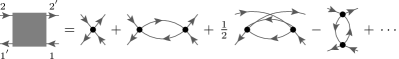
Figure 2: Diagrammatic expansion of the four-point vertex $\Gamma$ (square) up to second order in the interaction (i.e., these diagrams define $\Gamma^{\textrm{2nd}}$). The positions of the external (amputated) legs refer to the arguments of $\Gamma_{x_{1}^{\prime},x_{2}^{\prime};x_{1}^{\phantom{\prime}},x_{2}^{\phantom{\prime}}}$.

Following the conventions of Bickers Bickers (2004), the factor of $1/2$ in Eq. (8b) (Fig. 2) makes sure that, when summing over all internal indices, one does not overcount the effect of the two indistinguishable (parallel) lines. The minus sign in Eq. (8c) (Fig. 2) stems from the fact that the antiparallel bubbles (8a) and (8c) are related by exchange of fermionic legs. Indeed, using the antisymmetry of $\Gamma$ and $\Gamma^{\prime}$ in their arguments (crossing symmetry), we find

$$B_{a}(\Gamma,\Gamma^{\prime})_{x_{1}^{\prime},x_{2}^{\prime};x_{1}^{\phantom{\prime}},x_{2}^{\phantom{\prime}}}=-B_{t}(\Gamma,\Gamma^{\prime})_{x_{2}^{\prime},x_{1}^{\prime};x_{1}^{\phantom{\prime}},x_{2}^{\phantom{\prime}}}.\quad$$ (10)

The channel label $r\in\{a,p,t\}$ refers to the fact that the individual diagrams are reducible—i.e., they fall apart into disconnected diagrams—by cutting two antiparallel lines, two parallel lines, or two transverse (antiparallel) lines, respectively. (The term transverse itself refers to a horizontal space-time axis.) In using the terms antiparallel and parallel, we adopt the nomenclature used in the seminal application of the parquet equations to the X-ray-edge singularity by Roulet et al. Roulet et al. (1969). Equivalently, a common notation Rohringer et al. ; Wentzell et al. for the channels $a,p,t$ is $ph,pp,\overline{ph}$, referring to the (longitudinal) particle-hole, the particle-particle, and the transverse (or vertical) particle-hole channel, respectively. One also finds the labels $x,p,d$ in the literature Jakobs et al. (2010), referring to the so-called exchange, pairing, and direct channel, respectively.

In the context of fRG (cf. Sec. IV), functions such as $G$, $\Sigma$, $\Gamma$ develop a scale ($\Lambda$) dependence (which will be suppressed in the notation). If we write the bubble functions also symbolically as

$$B_{r}(\Gamma,\Gamma^{\prime}) =\big{[}\Gamma\circ G\circ G\circ\Gamma^{\prime}\big{]}_{r},$$ (11)

we can immediately define bubbles with differentiated propagators (but undifferentiated vertices) according to

$$\dot{B}_{r}(\Gamma,\Gamma^{\prime}) =\big{[}\Gamma\circ\big{(}\partial_{\Lambda}(G\circ G)\big{)}\circ\Gamma^{\prime}\big{]}_{r},$$ (12)

In the fRG flow equations, we will further need the (so-called) single-scale propagator, defined by ($\mathbbm{1}_{x,y}=\delta_{x,y}$)

$$S=\partial_{\Lambda}G|_{\Sigma=\textrm{const.}}=(\mathbbm{1}+G\cdot\Sigma)\cdot\big{(}\partial_{\Lambda}G^{0}\big{)}\cdot(\Sigma\cdot G+\mathbbm{1}).$$ (13)

Before moving on to the mfRG flow, let us next review the basics of the parquet formalism.

III Parquet formalism

The parquet formalism Bickers (2004); Roulet et al. (1969) provides exact, self-consistent equations for both four-point vertex and self-energy. Focusing on the vertex first, the central parquet equation represents a classification of diagrams distinguished by reducibility in the three two-particle channels:

$$\Gamma =R+\sum_{r}\gamma_{r},\quad I_{r}=R+\sum_{r^{\prime}\neq r}\gamma_{r^{\prime}}.$$ (14)

Diagrams of $\Gamma$ are either reducible in one of the three channels (i.e., part of $\gamma_{r}$ for $r\in\{a,p,t\}$, cf. Fig. 2), or they belong to the class of totally irreducible diagrams $R$ [cf. Fig. 3(a)]. (The notation again refers to Ref. Roulet et al., 1969.) As a diagram cannot simultaneously be reducible in more than one channel Roulet et al. (1969), one collects diagrams that are not reducible in $r$ lines into the irreducible vertex $I_{r}$ of that channel. Reducible and irreducible vertices are further related by the self-consistent Bethe-Salpeter equations (BSEs)

$$\gamma_{r} =B_{r}(I_{r},\Gamma),$$ (15)

the graphical representations of which are given in Fig. 4.

Figure 3: (a) Vertex diagram irreducible in all two-particle channels (i.e., it belongs to $R$) and thus not part of $\Gamma$ in the parquet approximation. (b) Schwinger-Dyson equation, relating the self-energy to the four-point vertex self-consistently.

The BSEs (15) are computed with full propagators $G$. Thus, they require knowledge of the self-energy, which itself can be determined by the self-consistent SDE depending on the four-point vertex [cf. Fig. 3(b)]:

$$\Sigma =L(\Gamma^{0},G)+L\big{[}B_{p}(\Gamma^{0},\Gamma),G\big{]}$$

$$=L(\Gamma^{0},G)+\tfrac{1}{2}L\big{[}B_{a}(\Gamma^{0},\Gamma),G\big{]}.$$ (16)

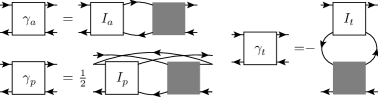
Figure 4: Bethe-Salpeter equations in the three two-particle channels, relating the reducible ($\gamma_{r}$) and irreducible ($I_{r}$) vertices self-consistently in the parquet formalism.

The only input required for solving the parquet equations is the totally irreducible vertex $R$. All remaining contributions to the vertex and self-energy are determined self-consistently. The simplest way to solve the parquet equations is to approximate $R$ by the bare vertex $\Gamma^{0}$. This is called the first-order parquet solution Roulet et al. (1969), or parquet approximation Bickers (2004), and corresponds to a summation of the leading logarithmic diagrams in logarithmically divergent perturbation theories.

The diagrams generated by the first-order parquet solution are called parquet diagrams. For $\Gamma$, these can be obtained by successively replacing bare vertices by one of the three bubbles from Eq. (8) (connected by full lines), starting from the bare vertex. For $\Sigma$, the parquet diagrams are obtained by inserting the parquet vertex into the SDE. They can also be characterized by the property that one needs to cut at most one bare line to obtain a parquet vertex with possible dressing at the external legs. By this, we mean that, instead of an ingoing or outgoing amputated leg, the external line is of the type $\mathbbm{1}+\Sigma\cdot G$ or $\mathbbm{1}+G\cdot\Sigma$, respectively, using again a parquet self-energy.

IV Multiloop fRG flow

The functional renormalization group Metzner et al. (2012); Kopietz et al. (2010) provides a hierarchy of exact flow equations for vertex functions, depending on an RG parameter $\Lambda$, serving as infrared cutoff in the bare propagator. A typical choice for the $\Lambda$ dependence, in order to flow from the trivially uncorrelated to the full theory, is characterized by the boundary conditions $G_{\Lambda_{i}}=0$ and $G_{\Lambda_{f}}=G$, implying $\Gamma_{\Lambda_{i}}=\Gamma^{0}$. Restring the flow to $\Sigma$ and $\Gamma$, the six-point vertex remains as input and is neglected in the standard approximation.

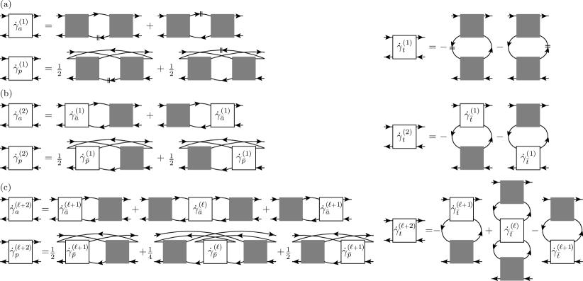
Figure 5: Multiloop flow equations for the four-point vertex in a general fermionic model. (a) Standard truncated, one-loop flow, where a line with double dashes denotes $\partial_{\Lambda}G$. (b) Two-loop correction (upon inserting the one-loop contributions, one obtains two loops connecting full vertices). (c) Higher-loop corrections starting from $\ell+2=3$, which contain the additional contribution (center part) where vertices from the complementary channels are connected by two bubbles.

Here, we view fRG as a tool to resum diagrams which does not necessarily rely on the original fRG hierarchy deduced from the flow of the (quantum) effective action. In previous works Kugler and von Delft (2018, ), we have used the X-ray-edge singularity as an example to show that the standard truncation of fRG restricts the flow to parquet diagrams of the vertex, and that the derivatives of those diagrams are only partially contained. Using the same model, we have introduced multiloop fRG flow equations for the vertex which complete the derivative of parquet diagrams in an iterative manner, as organized by the number of loops connecting full vertices, and thus do achieve a full summation of all parquet diagrams Kugler and von Delft (2018). The X-ray-edge singularity facilitates diagrammatic arguments as it allows one to consider only two two-particle channels and to neglect self-energies. Here, we give the details of how the mfRG flow of the vertex is generalized to all three two-particle channels with indistinguishable particles (as already indicated in Ref. Kugler and von Delft, 2018) and formulate the mfRG corrections to the self-energy flow (not discussed in Ref. Kugler and von Delft, 2018).

We first pose the mfRG flow equations and motivate them by showing examples of diagrams, which are otherwise only partially contained. Then, we justify the extensions of the truncated fRG flow by arguing that all diagrams are of the appropriate type without any overcounting. Subsequently, we give a recipe for counting the number of diagrams generated by the parquet and mfRG flow equations. This allows one to check that the mfRG flow fully captures all parquet diagrams order for order in the interaction. Finally, we discuss computational and general properties of the flow equations.

IV.1 Flow equations for the vertex

The mfRG flow of the vertex proposed in Ref. Kugler and von Delft, 2018 makes use of the channel classification known from the parquet equations and is organized by the loop order $\ell$. We write

$$\partial_{\Lambda}\Gamma=\sum_{r}\partial_{\Lambda}\gamma_{r},\ \partial_{\Lambda}\gamma_{r}=\sum_{\ell\geq 1}\dot{\gamma}_{r}^{(\ell)},\ \dot{\gamma}_{\bar{r}}^{(\ell)}=\sum_{r^{\prime}\neq r}\dot{\gamma}_{r^{\prime}}^{(\ell)},$$ (17)

where $\dot{\gamma}_{r}^{(\ell)}$ contains differentiated diagrams reducible in channel $r$ with $\ell$ loops connecting full vertices and will be constructed iteratively; $\bar{r}$ represents the complementary channels to channel $r$. Using the bubble functions (8) and the channel decomposition, the multiloop flow for $\Gamma$ is compactly stated as ($\ell\geq 1$)

$$\dot{\gamma}_{r}^{(1)} =\dot{B}_{r}(\Gamma,\Gamma),$$ (18a)

$$\dot{\gamma}_{r}^{(2)} =B_{r}\big{(}\dot{\gamma}_{\bar{r}}^{(1)},\Gamma\big{)}+B_{r}\big{(}\Gamma,\dot{\gamma}_{\bar{r}}^{(1)}\big{)},$$ (18b)

$$\dot{\gamma}_{r}^{(\ell+2)} =B_{r}\big{(}\dot{\gamma}_{\bar{r}}^{(\ell+1)},\Gamma\big{)}+\dot{\gamma}_{r,\textrm{C}}^{(\ell+2)}+B_{r}\big{(}\Gamma,\dot{\gamma}_{\bar{r}}^{(\ell+1)}\big{)},$$ (18c)

$$\dot{\gamma}_{r,\textrm{C}}^{(\ell+2)} =B_{r}\big{[}\Gamma,B_{r}\big{(}\dot{\gamma}_{\bar{r}}^{(\ell)},\Gamma\big{)}\big{]}=B_{r}\big{[}B_{r}\big{(}\Gamma,\dot{\gamma}_{\bar{r}}^{(\ell)}\big{)},\Gamma\big{]}$$ (18d)

and illustrated in Fig. 5.

The standard truncated, one-loop flow of $\Gamma$ is simply given by Eq. (18a) [Fig. 5(a)]. A simplified version of this equation, in which one uses the single-scale propagator $S$ (13) instead of $\partial_{\Lambda}G$ in the differentiated bubble (12), corresponds to the result obtained from the exact flow equation upon neglecting the six-point vertex . The form given here, with $\partial_{\Lambda}G$ instead of $S$ (also known as Katanin substitution Metzner et al. (2012); Katanin (2004)), already includes corrections to this originating from vertex diagrams containing differentiated self-energy contributions. In the exact flow equation, these contributions are contained in the six-point vertex $\Gamma^{(6)}$ and excluded in $S$; omitting $\Gamma^{(6)}$, they are incorporated again by $\partial_{\Lambda}G=S+G\cdot(\partial_{\Lambda}\Sigma)\cdot G$.

Comparing Eqs. (9), (11), (12) with Eq. (18a) [or Fig. 2 with Fig. 5(a)], it is clear that the one-loop flow is correct up to second order, for which only bare vertices are involved. Indeed, all differentiated diagrams of $\Gamma^{2^{\textrm{nd}}}$, which are obtained by summing all copies of diagrams in which one $G^{0}$ line is replaced by $\partial_{\Lambda}G^{0}$, are contained in $\sum_{r}\dot{\gamma}_{r}^{(1)}$. However, starting at third order, the one-loop flow (18a) does not fully generate all (parquet) diagrams, since, in the exact flow, the six-point vertex starts contributing. In mfRG, the two-loop flow [Eq. (18b), Fig. 5(b)] completes the derivative of third-order diagrams of $\Gamma$ (i.e., it contains all diagrams needed to ensure that $\dot{\gamma}_{r}^{(1)}+\dot{\gamma}_{r}^{(2)}$ fully represent $\partial_{\Lambda}\gamma_{r}^{\textrm{3rd}}$). An example is given in Fig. 6(a), which shows a parquet diagram reducible in channel $a$. The differentiated diagram in Fig. 6(d), as part of the derivative of Fig. 6(a), is not included in the one-loop flow. The reason is that $\dot{\gamma}_{a}^{(1)}$ only contains vertices connected by antiparallel $G^{0}$-$\partial_{\Lambda}G^{0}$ lines, and not parallel ones, as would be necessary for this differentiated diagram. It is, however, included in the two-loop correction to the flow, as can be seen by inserting the lowest-order contributions for all vertices into the first summand on the r.h.s. of $\dot{\gamma}_{a}^{(2)}$ (using $\dot{\gamma}_{p}^{(1)}$) in Fig. 5(b).

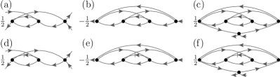
Figure 6: (a-c) Some diagrams that are included in the parquet approximation and only partially contained in one-loop fRG. (d-f) One particular differentiated diagram for each of the diagrams (a-c) [the (gray, thin) line with a dash stands for $\partial_{\Lambda}G^{0}$] that is not part of the standard truncated flow, but included in mfRG.

At all higher loop orders ($\ell+2\geq 3$) [Eq. (18c), Fig. 5(c)], we iterate this scheme and further add the center part (18d) of the vertex flow. This connects the $\ell$-loop flow from the complementary ($\bar{r}$) channels by $r$ bubbles on both sides, and is needed to complete the derivative of parquet diagrams starting at fourth order. Since $\dot{\gamma}_{r,\textrm{C}}^{(\ell+2)}$ raises the loop order by two, it was still absent in the two-loop flow. The three summands in $\dot{\gamma}_{r}^{(\ell+2)}$, including $\dot{\gamma}_{r,\textrm{C}}^{(\ell+2)}$, exhaust all possibilities to obtain differentiated vertex diagrams in channel $r$ at loop order $\ell+2$ in an iterative one-loop procedure. The mfRG vertex flow up to loop order $\ell$ therefore fully captures all parquet diagrams up to order $n=\ell+1$ in the interaction (cf. Sec. IV.4).

IV.2 Flow equation for the self-energy

The self-energy has an exact fRG flow equation, which simply connects the four-point vertex with the single-scale propagator (cf. Fig. 7). However, if a vertex obtained from the truncated vertex flow is inserted into this standard self-energy flow equation, it generates diagrams that are only partially differentiated. In fact, even after correcting the vertex flow via mfRG to obtain all parquet diagrams of $\Gamma$, $\dot{\Sigma}_{\textrm{std}}$ does not yet form a total derivative. Although $\dot{\Sigma}_{\textrm{std}}$ is in principle exact [as is the SDE (16)], using the parquet vertex in this flow gives a less accurate result than inserting it into the SDE: All diagrams obtained from $\dot{\Sigma}_{\textrm{std}}$ are of the parquet type, but their derivatives are not fully generated by the standard flow equation.

This problem can be remedied by adding multiloop corrections to the self-energy flow, which complete the derivative of all involved diagrams. The corrections consist of two additions that build on the center parts (18d) of the vertex flow in the $a$ and $p$ channels,

$$\dot{\gamma}_{\bar{t},\textrm{C}}=\sum_{\ell\geq 1}\big{(}\dot{\gamma}_{a,\textrm{C}}^{(\ell)}+\dot{\gamma}_{p,\textrm{C}}^{(\ell)}\big{)}.$$ (19)

Using the self-energy loop (5), the mfRG flow equation for $\Sigma$ is then given by (cf. Fig. 7)

$$\partial_{\Lambda}\Sigma =\dot{\Sigma}_{\textrm{std}}+\dot{\Sigma}_{\bar{t}}+\dot{\Sigma}_{t}, \dot{\Sigma}_{\textrm{std}} =L(\Gamma,S),$$ (20a)

$$\dot{\Sigma}_{\bar{t}} =L(\dot{\gamma}_{\bar{t},\textrm{C}},G), \dot{\Sigma}_{t} =L(\Gamma,G\cdot\dot{\Sigma}_{\bar{t}}\cdot G).$$ (20b)

Note that self-energy diagrams in $\dot{\Sigma}_{t}$ and $\dot{\Sigma}_{\bar{t}}$ are reducible and irreducible in the $t$ channel, respectively. However, here, this property is not exclusive; $\dot{\Sigma}_{\textrm{std}}$, too, contains diagrams that are reducible and irreducible in the $t$ channel, as is directly seen by inserting the second-order vertex from Fig. 2 into the first summand of Fig. 7.

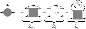
Figure 7: Multiloop flow equation for the self-energy, adding two corrections ($\dot{\Sigma}_{\bar{t}}$, $\dot{\Sigma}_{t}$) to the standard fRG flow, $\dot{\Sigma}_{\textrm{std}}$. The (black, thick) line with a dash denotes the single-scale propagator $S$.

To motivate the addition of $\dot{\Sigma}_{\bar{t}}$ and $\dot{\Sigma}_{t}$, let us consider the first examples where multiloop corrections are needed to complete the derivative of diagrams, which occur at fourth and fifth order, respectively. The diagram in Fig. 6(b) is obtained by inserting the $\gamma_{a}$ diagram from Fig. 6(a) (and the symmetry-related $\gamma_{t}$ diagram) into the SDE [Fig. 3(b)]. The differentiated diagram in Fig. 6(e) is part of the derivative of Fig. 6(b), but not contained in the standard flow. In fact, the vertex needed for this diagram to be part of $\dot{\Sigma}_{\textrm{std}}$ [i.e., the vertex obtained by cutting the differentiated line in Fig. 6(e)] is a so-called envelope vertex, the lowest-order realization of a nonparquet vertex [cf. Fig. 3(b)] . The diagram from Fig. 6(e) is, however, included in the first correction $\dot{\Sigma}_{\bar{t}}$, as can be seen by inserting the lowest-order contributions of all vertices in the center part of $\dot{\gamma}_{a}^{(3)}$ (using again $\dot{\gamma}_{p}^{(1)}$) in Fig. 5(c) and connecting the top lines.

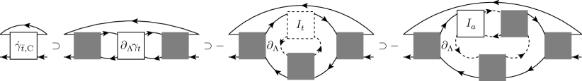
Figure 8: Special diagrams contributing to $\dot{\Sigma}_{\bar{t}}$. In the last two diagrams, we consider a scenario where the differentiated line is contained in one of the dashed contributions.

Inserting the self-energy diagram from Fig. 6(b) into the full propagator of the first summand in the SDE [Fig. 3(b)] yields the diagram in Fig. 6(c). Similar to the previous discussion, one finds that the differentiated diagram in Fig. 6(f), needed for the full derivative of Fig. 6(c), is neither contained in $\dot{\Sigma}_{\textrm{std}}$ nor $\dot{\Sigma}_{\bar{t}}$. It is, however, included in the second mfRG correction, $\dot{\Sigma}_{t}$, as one of the lowest-order realizations of the last summand in Fig. 7.

The two extra terms of the mfRG self-energy flow, $\dot{\Sigma}_{\bar{t}}$ and $\dot{\Sigma}_{t}$, incorporate the whole multiloop hierarchy of differentiated vertex diagrams via $\dot{\gamma}_{\bar{t},\textrm{C}}$ [Eq. (19)]. As is discussed in the following subsections, they suffice to generate all parquet diagrams of $\Sigma$ and, therefore, provide the full dressing of the parquet vertex in return.

IV.3 Justification

We will now justify our claim that the mfRG flow fully generates all parquet diagrams for $\Gamma$ and $\Sigma$. We will first show that all differentiated diagrams in mfRG are of the parquet type and that there is no overcounting of diagrams. Concerning the vertex, this has already been done for the two-channel case of the X-ray-edge singularity Kugler and von Delft (2018). The arguments for the general case are in fact completely analogous and repeated here for the sake of completeness. The self-energy is discussed thereafter.

The only totally irreducible contribution to the four-point vertex in the mfRG flow is the bare interaction stemming from the initial condition of the vertex, $\Gamma_{\Lambda_{i}}=\Gamma^{0}$. All further diagrams on the r.h.s. of the flow equations are obtained by iteratively combining two vertices by one of the three bubbles from Eq. (8). Hence, they correspond to differentiated parquet diagrams in the respective channel.

The fact that there is no overcounting in mfRG, i.e., that each diagram occurs at most once, can be seen employing arguments of diagrammatic reducibility and the unique position of the differentiated line in the diagrams. To be specific, let us consider here the $a$ channel; the arguments for the other channels are completely analogous.

First, we note that diagrams in the one-loop term always differ from higher-loop ones. The reason is that, in higher-loop terms, the differentiated line appears in the vertex coming from $\partial_{\Lambda}\gamma_{\bar{a}}$. This can never contain two vertices connected by an $a$ $G$-$\partial_{\Lambda}G$ bubble, since such terms only originate upon differentiating $\gamma_{a}$, the vertex reducible in $a$ lines.

Second, diagrams in the left, center, or right part [first, second, and third summand in Fig. 5(c), respectively] of an $\ell$-loop contribution always differ. This is because the vertex $\gamma^{(\ell)}_{\bar{a}}$ is irreducible in $a$ lines. The left part is then reducible in $a$ lines only after the differentiated line appeared, the right part only before, and the center part is reducible in this channel before and after $\partial_{\Lambda}G$.

Third, the same parts (say, the left parts) of different-order loop contributions ($\ell\neq\ell^{\prime}$) are always different. Assume they agreed: As the $a$ bubble induces the first reducibility in this channel, already $\gamma^{(\ell)}_{\bar{a}}$ and $\gamma^{(\ell^{\prime})}_{\bar{a}}$ would have to agree. For these, only the same parts can agree, as mentioned before. The argument then proceeds iteratively until one compares the one-loop part to a higher-loop ($|\ell-\ell^{\prime}|+1$) one. These are, however, distinct according to the first point.

Concerning the self-energy, all diagrams of the flow belong to the parquet type, since they are constructed from (differentiated) parquet vertices by closing loops of external legs in an iterative one-loop procedure. By cutting one $G^{0}$ or the $\partial_{\Lambda}G^{0}$ line in such a self-energy diagram, one can always obtain a (differentiated) parquet vertex with possibly dressed amputated legs.

First, there is no overcounting between $\dot{\Sigma}_{\textrm{std}}$ and $\dot{\Sigma}_{\bar{t}}$ because cutting the differentiated line in $\dot{\Sigma}_{\textrm{std}}$ generates a parquet vertex (with possibly dressed amputated legs coming from the single-scale propagator; cf. Fig. 7), whereas this is not the case for $\dot{\Sigma}_{\bar{t}}$. To illustrate this statement, we consider in Fig. 8 a typical case of a $\dot{\Sigma}_{\bar{t}}$ correction, where we take the $a$ part of $\dot{\gamma}_{\bar{t},\textrm{C}}$ [cf. Eq. (19)] with $\partial_{\Lambda}\gamma_{t}$ in the center. We can insert the BSE $\gamma_{t}=B_{t}(I_{t},\Gamma)$ (Fig. 4) and consider simultaneously all scenarios where the differentiated line, originating from $\partial_{\Lambda}\gamma_{t}$, is contained in any of the dashed parts. To be even more specific, we take a specific part of $I_{t}=R+\gamma_{a}+\gamma_{p}$, namely $\gamma_{a}=B_{a}(I_{a},\Gamma)$ (Fig. 4), and consider the cases where the differentiated line, if contained in $I_{t}$, is contained in the corresponding bubble. If one now cuts any of the dashed lines, as candidates for the differentiated line, one finds that the remaining vertex is not of the parquet type, as it is not reducible in any of the two-particle channels. The same irreducibility in three lines, when starting to cut the differentiated line in $\dot{\gamma}_{\bar{t},\textrm{C}}$, occurs in all diagrammatic realizations of $\dot{\Sigma}_{\bar{t}}$.

Since the standard flow $\dot{\Sigma}_{\textrm{std}}$ with the full instead of the parquet vertex is exact, it follows that the $\dot{\Sigma}_{\bar{t}}$ part can be written similarly as $\dot{\Sigma}_{\textrm{std}}$, but using a nonparquet (np) vertex [Fig. 9(a)]. As a consequence, $\dot{\Sigma}_{t}$, obtained by connecting $\dot{\Sigma}_{\bar{t}}$ and $\Gamma$ by a $t$ bubble, can similarly be written with a nonparquet vertex [Fig. 9(b)]. Thus, there cannot be any overcounting between $\dot{\Sigma}_{\textrm{std}}$ and $\dot{\Sigma}_{t}$, either. Finally, there is likewise no overcounting between $\dot{\Sigma}_{\bar{t}}$ and $\dot{\Sigma}_{t}$: After removing the differentiated line in $\dot{\Sigma}_{\bar{t}}$, the remaining nonparquet vertex $\Gamma_{\textrm{np}}$ is in particular irreducible in the $t$ channel (as was discussed above). However, removing the differentiated line in $\dot{\Sigma}_{t}$ after expressing $\dot{\Sigma}_{\bar{t}}$ via $\Gamma_{\textrm{np}}$ [cf. Fig. 9(b)], the remaining vertex $\Gamma^{\prime}_{\textrm{np}}$ is by construction reducible in $t$ lines (although not a parquet vertex).

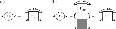
Figure 9: Rewriting of the corrections to the self-energy flow: (a) $\dot{\Sigma}_{\bar{t}}$ can be expressed by a nonparquet vertex $\Gamma_{\textrm{np}}$ contracted with the single-scale propagator $S$. (b) $\dot{\Sigma}_{t}$, obtained by connecting $\dot{\Sigma}_{\bar{t}}$ and $\Gamma$ by a $t$ bubble, then involves a bubble connecting a nonparquet and parquet vertex, which yields another nonparquet vertex $\Gamma^{\prime}_{\textrm{np}}$, contracted with $S$.

In summary, all diagrams of the four-point vertex and self-energy generated by the mfRG flow belong to the parquet class and are included at most once. To show that the mfRG flow generates all differentiated parquet diagrams, we will demonstrate next that, at any given order in the interaction, their number is equal to the number of diagrams generated by the mfRG flow.

IV.4 Counting of diagrams

In order to count the number of diagrams in all involved functions, we make use of either exact, self-consistent equations or the mfRG flow equations. As a first example, we count the number of diagrams in the full propagator $G$ at order $n$ in the interaction, $\mathcal{N}_{G}(n)$, given the number of diagrams in the self-energy, $\mathcal{N}_{\Sigma}(n)$. Concerning the bare propagator and self-energy, we know $\mathcal{N}_{G^{0}}(n)=\delta_{n,0}$ and $\mathcal{N}_{\Sigma}(0)=0$. From Dyson’s equation (4), we then get

$$\mathcal{N}_{G}(n)=\delta_{n,0}+\sum_{m=1}^{n}\mathcal{N}_{\Sigma}(m)\mathcal{N}_{G}(n-m).$$ (21)

Defining a convolution of sequences, according to

$$\mathcal{N}_{1}=\mathcal{N}_{2}\ast\mathcal{N}_{3}\ \Leftrightarrow\ \mathcal{N}_{1}(n)=\sum_{m=0}^{n}\mathcal{N}_{2}(m)\mathcal{N}_{3}(n-m)\ \forall n,$$ (22)

we can write Eq. (21) in direct analogy to the original equation (4) as

$$\mathcal{N}_{G}=\mathcal{N}_{G^{0}}+\mathcal{N}_{G^{0}}\ast\mathcal{N}_{\Sigma^{\vphantom{(6)}}}\ast\mathcal{N}_{G^{\vphantom{(6)}}}.$$ (23)

Similar relations for the self-energy and vertex can be obtained from the SDE (16), the parquet equation (14), and the BSEs (15). The number of diagrams in the bare vertex is $\mathcal{N}_{\Gamma^{0}}=\delta_{n,1}$ (one can also take any $\mathcal{N}_{\Gamma^{0}}\propto\delta_{n,1}$). From the SDE (16), we get for the self-energy

$$\mathcal{N}_{\Sigma}=\mathcal{N}_{\Gamma^{0}}\ast\mathcal{N}_{G^{\vphantom{(6)}}}+\tfrac{1}{2}\,\mathcal{N}_{\Gamma^{0}}\ast\mathcal{N}_{G^{\vphantom{(6)}}}\ast\mathcal{N}_{G^{\vphantom{(6)}}}\ast\mathcal{N}_{G^{\vphantom{(6)}}}\ast\mathcal{N}_{\Gamma^{\vphantom{(6)}}}.$$ (24)

Note that, when counting diagrams, we can ignore the extra minus signs but must keep track of prefactors of magnitude not equal to unity. These prefactors avoid double counting of the antisymmetric vertex Bickers (2004) and originate from the way the diagrams are constructed .

Concerning the full vertex, we can use that the symmetry relation between the $a$ and $t$ bubble given in Eq. (10) holds for the full reducible vertices $\gamma_{a}$ and $\gamma_{t}$ Bickers (2004), such that $\mathcal{N}_{\gamma_{a}}=\mathcal{N}_{\gamma_{t}}$. In the parquet approximation $R=\Gamma^{0}$, and the parquet equation (14) and the BSEs (15) yield

$$\mathcal{N}_{\Gamma} =\mathcal{N}_{R}+2\,\mathcal{N}_{\gamma_{a}}+\mathcal{N}_{\gamma_{p}}$$ (25a)

$$\mathcal{N}_{\gamma_{a}} =(\mathcal{N}_{\Gamma}-\mathcal{N}_{\gamma_{a}})\ast\mathcal{N}_{G}\ast\mathcal{N}_{G}\ast\mathcal{N}_{\Gamma}$$ (25b)

$$\mathcal{N}_{\gamma_{p}} =\tfrac{1}{2}(\mathcal{N}_{\Gamma}-\mathcal{N}_{\gamma_{p}})\ast\mathcal{N}_{G}\ast\mathcal{N}_{G}\ast\mathcal{N}_{\Gamma}.$$ (25c)

Since $\mathcal{N}_{\Gamma^{0}}(0)=0$, these equations, just like the original equations, can be solved iteratively. Knowing the number of diagrams in all quantities up to order $n-1$ allows one to calculate them at order $n$. This can also be done numerically. Table 1 (first two lines) shows the number of parquet diagrams up to order 6. For large interaction order $n$, we find that the number of diagrams in the parquet vertex and self-energy grows exponentially in $n$ [cf. Fig. 10(a)].

To prove our claim that the mfRG flow generates all parquet diagrams, we must count the number of diagrams, $\mathcal{N}_{\dot{\Sigma}}(n)$ and $\mathcal{N}_{\dot{\gamma}_{r}}(n)$, obtained by differentiating the set of all corresponding parquet graphs. Then, we check that these numbers are exactly reproduced by the number of diagrams contained on the r.h.s. of the mfRG flow equations. A diagram of the full propagator at order $n$ has $2n+1$ internal lines, a self-energy diagram $2n-1$, and vertex diagram $2n-2$. According to the product rule, the number of differentiated diagrams is thus

$$\mathcal{N}_{\dot{G}}(n) =\mathcal{N}_{G}(n)(2n+1),$$ (26a)

$$\mathcal{N}_{\dot{\Sigma}}(n) =\mathcal{N}_{\Sigma}(n)(2n-1),$$ (26b)

$$\mathcal{N}_{\dot{\gamma}_{r}}(n) =\mathcal{N}_{\gamma_{r}}(n)(2n-2).$$ (26c)

$n$	1	2	3	4	5	6
$\mathcal{N}_{\Gamma}$	1	2$\frac{1}{2}$	15$\tfrac{1}{4}$	108$\tfrac{1}{8}$	832$\tfrac{1}{16}$	6753$\tfrac{21}{32}$
$\mathcal{N}_{\Sigma}$	1	1$\frac{1}{2}$	5$\frac{1}{4}$	25$\frac{7}{8}$	156$\frac{1}{16}$	1073$\frac{3}{32}$
$\mathcal{N}_{\dot{\Gamma}}$	0	5	61	648$\frac{3}{4}$	6656$\frac{1}{2}$	67536$\frac{9}{16}$
$\mathcal{N}_{\dot{\Gamma}^{(1\ell)}}$	0	5	45	373$\frac{3}{4}$	3117$\frac{1}{2}$	26519$\frac{1}{16}$
$\mathcal{N}_{\dot{\Gamma}^{(2\ell)}}$	0	0	16	216	2264	21972
$\mathcal{N}_{\dot{\Gamma}^{(3\ell)}}$	0	0	0	59	1062	13481$\frac{1}{2}$
$\mathcal{N}_{\dot{\Gamma}^{(4\ell)}}$	0	0	0	0	213	4792$\frac{1}{2}$
$\mathcal{N}_{\dot{\Gamma}^{(5\ell)}}$	0	0	0	0	0	771$\frac{1}{2}$
$\mathcal{N}_{\dot{\Sigma}}$	1	4$\frac{1}{2}$	26$\frac{1}{4}$	181$\frac{1}{8}$	1404$\frac{9}{16}$	11804$\frac{1}{32}$
$\mathcal{N}_{\dot{\Sigma}_{\textrm{std}}}$	1	4$\frac{1}{2}$	26$\frac{1}{4}$	177$\frac{1}{8}$	1311$\frac{9}{16}$	10348$\frac{1}{32}$
$\mathcal{N}_{\dot{\Sigma}_{\bar{t}}}$	0	0	0	4	89	1349
$\mathcal{N}_{\dot{\Sigma}_{t}}$	0	0	0	0	4	107

Table 1: Number of (bare) parquet diagrams, differentiated parquet diagrams, and diagrams generated by mfRG up to interaction order 6 and loop order 5. Fractional parts originate from multiple factors of $1/2$, used to avoid double counting of the antisymmetric vertex Bickers (2004). As we use $\mathcal{N}_{\Gamma^{0}}=\delta_{n,1}$, we count Hugenholtz diagrams Negele and Orland (1998) [where, e.g., $\mathcal{N}_{\Sigma}(1)=1$, cf. Fig. 1]. The choice $\mathcal{N}_{\Gamma^{0}}=2\delta_{n,1}$ [cf. Eq. (2b)] would give an extra factor $2^{n}$ for all numbers of diagrams at order $n$, resulting in the (integer) numbers of Feynman diagrams [where, e.g., $\mathcal{N}_{\Sigma}(1)=2$].

From the mfRG flow of the vertex [Eq. (18)], we deduce

$$\mathcal{N}_{\dot{\gamma}_{a}^{(1)}} =2\,\mathcal{N}_{\Gamma\vphantom{\dot{G}}}\ast\mathcal{N}_{\dot{G}}\ast\mathcal{N}_{G\vphantom{\dot{G}}}\ast\mathcal{N}_{\Gamma\vphantom{\dot{G}}},$$ (27a)

$$\mathcal{N}_{\dot{\gamma}_{p}^{(1)}} =\mathcal{N}_{\Gamma\vphantom{\dot{G}}}\ast\mathcal{N}_{\dot{G}}\ast\mathcal{N}_{G\vphantom{\dot{G}}}\ast\mathcal{N}_{\Gamma\vphantom{\dot{G}}},$$ (27b)

$$\mathcal{N}_{\dot{\gamma}_{a}^{(2)}} =2\,(\mathcal{N}_{\dot{\gamma}^{(1)}_{a}}+\mathcal{N}_{\dot{\gamma}^{(1)}_{p}})\ast\mathcal{N}_{\Pi}\ast\mathcal{N}_{\Gamma},$$ (27c)

$$\mathcal{N}_{\dot{\gamma}_{p}^{(2)}} =2\,\mathcal{N}_{\dot{\gamma}^{(1)}_{a}}\ast\mathcal{N}_{\Pi}\ast\mathcal{N}_{\Gamma},$$ (27d)

where $\mathcal{N}_{\Pi}=\mathcal{N}_{G}\ast\mathcal{N}_{G}$ denotes the number of diagrams in a bubble. For $\ell+2\geq 3$, we have

$$\mathcal{N}_{\dot{\gamma}_{a}^{(\ell+2)}} =2\,(\mathcal{N}_{\dot{\gamma}^{(\ell+1)}_{a}}+\mathcal{N}_{\dot{\gamma}^{(\ell+1)}_{p}})\ast\mathcal{N}_{\Pi}\ast\mathcal{N}_{\Gamma}$$

$$\ +\mathcal{N}_{\Gamma}\ast\mathcal{N}_{\Pi}\ast(\mathcal{N}_{\dot{\gamma}^{(\ell)}_{a}}+\mathcal{N}_{\dot{\gamma}^{(\ell)}_{p}})\ast\mathcal{N}_{\Pi}\ast\mathcal{N}_{\Gamma},$$ (28a)

$$\mathcal{N}_{\dot{\gamma}_{p}^{(\ell+2)}} =2\,\mathcal{N}_{\dot{\gamma}^{(\ell+1)}_{a}}\ast\mathcal{N}_{\Pi}\ast\mathcal{N}_{\Gamma}$$

$$\ +\tfrac{1}{2}\,\mathcal{N}_{\Gamma}\ast\mathcal{N}_{\Pi}\ast\mathcal{N}_{\dot{\gamma}^{(\ell)}_{a}}\ast\mathcal{N}_{\Pi}\ast\mathcal{N}_{\Gamma}.$$ (28b)

Summing all loop contributions yields

$$\textstyle\mathcal{N}_{\dot{\gamma}_{a}}^{\textrm{mfRG}}=\sum_{\ell\geq 1}\mathcal{N}_{\dot{\gamma}^{(\ell)}_{a}},\quad\mathcal{N}_{\dot{\gamma}_{p}}^{\textrm{mfRG}}=\sum_{\ell\geq 1}\mathcal{N}_{\dot{\gamma}^{(\ell)}_{p}}.$$ (29)

For the flow of the self-energy (20), we need the center part of the vertex flow in the $a$ and $p$ channel, for which the number of diagrams sums up to

$$\mathcal{N}_{\dot{\gamma}_{\bar{t},\textrm{C}}} =\mathcal{N}_{\Gamma}\ast\mathcal{N}_{\Pi}\ast\Big{(}\tfrac{3}{2}\,\mathcal{N}_{\dot{\gamma}_{a}}^{\textrm{mfRG}}+\mathcal{N}_{\dot{\gamma}_{p}}^{\textrm{mfRG}}\Big{)}\ast\mathcal{N}_{\Pi}\ast\mathcal{N}_{\Gamma}.$$ (30)

The number of diagrams in the single-scale propagator $S$ (13) can be obtained from two equivalent relations

$$\mathcal{N}_{S\vphantom{\dot{G}}} =\mathcal{N}_{\dot{G}}-\mathcal{N}_{G\vphantom{\dot{G}}}\ast N_{\dot{\Sigma}}\ast\mathcal{N}_{G\vphantom{\dot{G}}}$$ (31a)

$$=(\mathcal{N}_{\mathbbm{1}\vphantom{\dot{G}}}+\mathcal{N}_{G\vphantom{\dot{G}}}\ast\mathcal{N}_{\Sigma\vphantom{\dot{G}}})\ast\mathcal{N}_{\dot{G}^{0}}\ast(\mathcal{N}_{\mathbbm{1}\vphantom{\dot{G}}}+\mathcal{N}_{\Sigma\vphantom{\dot{G}}}\ast\mathcal{N}_{G\vphantom{\dot{G}}}),$$ (31b)

with $\mathcal{N}_{\dot{G}^{0}}(n)=\delta_{n,0}=\mathcal{N}_{\mathbbm{1}}(n)$. From Eq. (20), we then get

$$\mathcal{N}_{\dot{\Sigma}}^{\textrm{mfRG}} =\mathcal{N}_{\dot{\Sigma}_{\textrm{std}}}+\mathcal{N}_{\dot{\Sigma}_{\bar{t}}}+\mathcal{N}_{\dot{\Sigma}_{t}}, \mathcal{N}_{\dot{\Sigma}_{\textrm{std}}} =\mathcal{N}_{\Gamma\vphantom{\dot{G}}}\ast\mathcal{N}_{S\vphantom{\dot{G}}},$$

$$\mathcal{N}_{\dot{\Sigma}_{\bar{t}}} =\mathcal{N}_{\dot{\gamma}_{\bar{t},\textrm{C}}}\ast\mathcal{N}_{G\vphantom{\dot{G}}}, \mathcal{N}_{\dot{\Sigma}_{t}} =\mathcal{N}_{\Gamma\vphantom{\dot{G}}}\ast\mathcal{N}_{\Pi\vphantom{\dot{G}}}\ast\mathcal{N}_{\dot{\Sigma}_{\bar{t}}}.$$ (32)

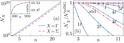
Figure 10: Logarithmic plots for the number of diagrams at interaction order $n$ for both vertex and self-energy. (a) $\mathcal{N}_{\Gamma}$, $\mathcal{N}_{\Sigma}$ grow exponentially for large $n$ (inset: the ratio of subsequent elements approaches a constant). (b) The cumulative low-loop vertex flows ($1\ell$ up to $5\ell$) and the self-energy flows $\dot{\Sigma}_{\textrm{std}}$ (labeled std) and $\dot{\Sigma}_{\textrm{std}}+\dot{\Sigma}_{\bar{t}}$ (labeled $\bar{t}$) miss differentiated parquet diagrams. However, the full multiloop flow for vertex and self-energy generates all differentiated parquet diagrams to arbitrary order in the interaction.

Numerically, one can check order for order in the interaction [cf. Table 1 and Fig. 10(b)] that, indeed, the mfRG flow generates exactly the same number of diagrams as obtained by differentiating all parquet diagrams, i.e.,

$$\mathcal{N}_{\dot{\gamma}_{r}}^{\textrm{\vphantom{G}}}(n) =\mathcal{N}_{\dot{\gamma}_{r}}^{\textrm{mfRG}}(n),\quad\mathcal{N}_{\dot{\Sigma}}^{\textrm{\vphantom{G}}}(n)=\mathcal{N}_{\dot{\Sigma}}^{\textrm{mfRG}}(n)\quad\forall n.$$ (33)

This demonstrates the equivalence between solving the multiloop fRG flow and solving the (first-order) parquet equations for a general model.

IV.5 Computational aspects

All contributions to the mfRG flow—for the vertex as well as for the self-energy—are of an iterative one-loop structure and hence well suited for numerical algorithms. In fact, by keeping track of the left (L) and right (R) summands in the higher-loop vertex flow (18c)

$$\dot{\gamma}_{r,\textrm{L}}^{(\ell+2)}=B_{r}\big{(}\gamma_{\bar{r}}^{(\ell+1)},\Gamma\big{)},\quad\dot{\gamma}_{r,\textrm{R}}^{(\ell+2)}=B_{r}\big{(}\Gamma,\gamma_{\bar{r}}^{(\ell+1)}\big{)},$$ (34)

the center part (18d) can be efficiently computed as

$$\dot{\gamma}_{r,\textrm{C}}^{(\ell+2)}=B_{r}\big{(}\Gamma,\gamma_{r,\textrm{L}}^{(\ell+1)}\big{)}=B\big{(}\gamma_{r,\textrm{R}}^{(\ell+1)},\Gamma\big{)}.$$ (35)

Consequently, the numerical effort in the multiloop corrections of the vertex flow scales linearly in $\ell$. The self-energy flow (20) is already stated with one integration only.

The (standard) fRG hierarchy of flow equations constitutes a (first-order) ordinary differential equation. Neglecting the six-point vertex, it can be written as

$$\partial_{\Lambda}\Sigma=f_{\Sigma}^{\textrm{std}}(\Lambda,\Sigma,\Gamma),\quad\partial_{\Lambda}\Gamma=f_{\Gamma}^{\textrm{std}}(\Lambda,\Sigma,\Gamma),$$ (36)

where, here and henceforth, $f$ denotes the part of the r.h.s. of the flow equation corresponding to its indices. Improving this approximation by adding differentiated self-energy contributions in the vertex flow (as is also done in mfRG), $f_{\Gamma}^{\textrm{std}}$ is replaced by another function $\tilde{f}_{\Gamma}^{\textrm{std}}(\Lambda,\Sigma,\Gamma,\partial_{\Lambda}\Sigma)$, which further depends on the $\Lambda$ derivative of the self-energy. Such a differential equation is still feasible for many algorithms as one can simply compute $\partial_{\Lambda}\Sigma$ first and use it in the calculation of $\partial_{\Lambda}\Gamma$. However, the full mfRG flow for the vertex and self-energy has the form

$$\partial_{\Lambda}\Sigma=f_{\Sigma}(\Lambda,\Sigma,\Gamma,\partial_{\Lambda}\Gamma),\quad\partial_{\Lambda}\Gamma=f_{\Gamma}(\Lambda,\Sigma,\Gamma,\partial_{\Lambda}\Sigma),$$ (37)

in which derivatives occur on all parts of the r.h.s., yielding an algebraic (as opposed to ordinary) differential equation.

Techniques to solve algebraic differential equations exist, but a discussion of them exceeds the scope of this paper. Let us merely suggest an approximate solution strategy that reduces the mfRG flow to an ordinary differential equation, has no computational overhead, and deviates from the exact flow starting at sixth order in the interaction, summarized as follows:

$$\dot{\Sigma}_{\textrm{std}} =f_{\dot{\Sigma}_{\textrm{std}}}(\Lambda,\Sigma,\Gamma),$$ (38a)

$$\partial_{\Lambda}\Gamma \approx\dot{\Gamma}_{\textrm{approx}}=f_{\Gamma}(\Lambda,\Sigma,\Gamma,\partial_{\Lambda}\Sigma=\dot{\Sigma}_{\textrm{std}}),$$ (38b)

$$\partial_{\Lambda}\Sigma \approx\dot{\Sigma}_{\textrm{std}}+f_{\dot{\Sigma}_{\bar{t}}}(\Lambda,\Sigma,\partial_{\Lambda}\Gamma=\dot{\Gamma}_{\textrm{approx}})$$

$$\ +f_{\dot{\Sigma}_{t}}(\Lambda,\Sigma,\partial_{\Lambda}\Gamma=\dot{\Gamma}_{\textrm{approx}}).$$ (38c)

According to this scheme, one computes first the standard flow of the self-energy, which deviates from the full $\Sigma$ flow at interaction order $U^{4}$. Inserting this into the vertex flow yields an approximate vertex derivative, $\dot{\Gamma}_{\textrm{approx}}$, where deviations from the full flow, induced by the approximate form of $\partial_{\Lambda}\Sigma$, start at order $U^{6}$. The center part of the vertex flow involves at least four vertices, such that deviations, induced by the self-energy, start at order $U^{8}$. The resulting, approximate $\dot{\gamma}_{\bar{t},\textrm{C}}$ can then be used to complete $\partial_{\Lambda}\Sigma$, adding the terms $\dot{\Sigma}_{\bar{t}}$ and $\dot{\Sigma}_{t}$, such that the self-energy flow is correctly computed up to errors of order $U^{8}$. Evidently, this scheme can also be iterated [using Eqs. (38b) and (38c)], increasing the accuracy by four orders with each step. We have attached a pseudocode for such a solution strategy of the mfRG flow in Appendix A.

IV.6 General aspects

Since the standard fRG flow for the self-energy and four-point vertex—including the six-point vertex—is exact, all mfRG corrections can be understood as fully simulating the effect of the six-point vertex on parquet diagrams of $\Sigma$ and $\Gamma$. For instance, the two-loop corrections to the vertex flow and the Katanin substitution in the improved one-loop flow equation contain all third-order contributions of the six-point vertex Kugler and von Delft ; Katanin (2004); Eberlein (2014). Nevertheless, in the standard fRG hierarchy of flow equations, the parquet graphs comprise $n$-point vertices of arbitrary order ($n$) Kugler and von Delft , such that a non-diagrammatic derivation of mfRG based on this hierarchy appears rather difficult. Conversely, the derivation of the mfRG flow does not rely on the fRG hierarchy or properties of the (quantum) effective action; it can thus be understood independently and without prior knowledge of fRG.

The mfRG flow at the two- or higher-loop level is exact up to third order in the interaction and therefore naturally fulfills Ward identities with accuracy $\textit{O}(\Gamma^{4})$, compared to $\textit{O}(\Gamma^{3})$ in the case of one-loop fRG Katanin (2004). Yet, since the parquet self-energy is exact up to fourth order but the parquet vertex only up to third order, such identities are typically violated starting at fourth order. One can think of schemes to extend mfRG beyond the parquet approximation. However, we find those rather impracticable and only briefly mention them in Appendix B.

Furthermore, the mfRG flow is applicable for any initial condition of the vertex functions. Whereas the choice $G_{\Lambda_{i}}=0$ used here leads to a summation of all parquet diagrams, starting the mfRG flow from the local quantities of dynamical mean-field theory (DMFT) Georges et al. (1996); Taranto et al. (2014) allows one to add nonlocal correlations, similarly to solving the parquet equations in the dynamical vertex approximation (D$\Gamma$A) Toschi et al. (2007); Held et al. (2008); Valli et al. (2010). However, contrary to D$\Gamma$A, the mfRG flow is built on the full vertex $\Gamma^{(4)}_{\textrm{DMFT}}$ and does not require the diagrammatic decomposition of the nonperturbative vertex $\Gamma^{(4)}_{\textrm{DMFT}}=R+\sum_{r}\gamma_{r}$ that leads to diverging results close to a quantum phase transition Schäfer et al. (2013, 2016); Gunnarsson et al. (2017).

Inspecting the one-loop flow equations of the vertex once more, we observe that diagrams on the r.h.s. contain the differentiated propagator only in the two-particle lines that induce the reducibility. Propagators which appear in two-particle lines which do not induce the reducibility are not differentiated. Therefore, only those diagrams that are reducible in all positions of two-particle lines—the so-called ladder diagrams—are fully included. It follows that the standard truncated, one-loop fRG flow is biased towards ladder constructions of the four-point vertex.

For a constant interaction $U$ and a transfer energy-momentum $\Omega$, ladder diagrams of a certain channel can easily be summed to $\Gamma^{\textrm{ladder}}_{\Omega}=U(1-U\Pi_{\Omega})^{-1}$, where $\Pi_{\Omega}$ is the corresponding bubble. Ladder diagrams are therefore particularly prone to divergences with increasing $U$ or increasing values of $\Pi_{\Omega}$ (as can occur upon lowering the cutoff scale $\Lambda$) and can thus be responsible for premature vertex divergences in fRG. Indeed, so far, fRG computations have often suffered from such vertex divergences, and the flow had be stopped at finite RG scale $\Lambda_{c}$ Metzner et al. (2012); Eberlein and Metzner (2014). In this context, the two-loop corrections have been found to significantly reduce the critical scale of vertex divergences $\Lambda_{c}$ Eberlein (2014); Rueck and Reuther . This suggests that it would be worthwhile to study the effect of higher-loop mfRG corrections—we expect that they reduce $\Lambda_{c}$ even further.

Throughout this paper, we have taken a perspective that views fRG as a tool to resum diagrams (say, physical diagrams) by integrating a collection of differentiated (and thus $\Lambda$-dependent) diagrams. In this regard, the mfRG corrections do not add new physical diagrams to the flow, they only add differentiated diagrams to complete those derivatives of physical diagrams that are only partially contained by one-loop fRG. In other words, for any physical diagram to which a differentiated diagram of mfRG contributes, there also exists a differentiated diagram in one-loop fRG. The differentiated diagrams of the higher-loop corrections and the one-loop flow all contribute the same set of physical diagrams—the parquet diagrams.

Whereas the one-loop flow of the vertex contains differentiated propagators at the two-particle-reducible positions, the multiloop flow iteratively adds those parts for which the differentiated line is increasingly nested. Such non-ladder contributions are crucial to suppress vertex divergences originating from the summation of ladder diagrams Kugler and von Delft (2018). Similarly, the standard self-energy flow does not form a total derivative any more if one has only the parquet vertex at one’s disposal. All diagrams of the standard flow are of the parquet type, but differentiated lines in heavily nested positions are omitted (cf. Fig. 6). The mfRG corrections incorporate all remaining contributions by two additions that build up on the multiloop vertex flow. Altogether, the mfRG flow achieves a full summation of all parquet diagrams of the vertex and self-energy. Consequently, mfRG solutions are no longer dependent on the specific way the $\Lambda$ dependence (regulator) was introduced Kugler and von Delft (2018) and thus fully implement the meaning of the original fRG idea.

V Conclusion

We have presented multiloop fRG flow equations for the four-point vertex and self-energy, formulated for the general fermionic many-body problem. The mfRG corrections fully simulate the effect of the six-point vertex on parquet diagrams, completing the derivatives of diagrams that are only partially contained in the standard truncated fRG flow. Whereas one-loop fRG contains differentiated propagators only at the two-particle-reducible positions and the standard self-energy flow does not suffice to form a total derivative when having only the parquet vertex at one’s disposal, the multiloop iteration adds all remaining parts, where the differentiated line appears at increasingly nested positions. We have motivated the multiloop corrections at low orders and ruled out any overcounting of diagrams. Moreover, we have put forward a simple recipe to count diagrams and numerically check that the mfRG flow generates all differentiated parquet diagrams for the vertex and self-energy, order for order in the interaction.

Due to its iterative one-loop structure, the mfRG flow is well suited for efficient numerical computations. We have given a simple approximation, which renders the algebraic differential equation accessible to standard solvers for ordinary differential equations and exhibits only minor deviations from the full mfRG flow. Given the general formulation, the benefits of mfRG on physical problems can be exploited in a large number of fRG applications. The full resummation of parquet diagrams via mfRG eliminates the bias of fRG computations towards divergent ladder constructions of the vertex and restores the independence on the choice of regulator. We expect that this will generically enhance the usefulness of the truncated fRG framework and increase the robustness of the physical conclusions drawn from fRG results.

Appendix A Pseudocode implementation

1: Function $f(\Lambda,\Psi$):

1:$S=S(\Lambda,\Psi.\Sigma)$

2:$G=G(\Lambda,\Psi.\Sigma)$

3:$\textrm{d}\Sigma_{\textrm{std}}=L(\Psi.\Gamma,S)$

4:$\textrm{d}\Psi.\Sigma=\textrm{d}\Sigma_{\textrm{std}}$

5:for $it=1\dots it_{f}$ do

6:   $\textrm{d}G=S+G\cdot\textrm{d}\Psi.\Sigma\cdot G$

7:   for $r=a,p,t$ do

8:      $\textrm{d}\gamma_{r}=\dot{B}_{r}(\Psi.\Gamma,\Psi.\Gamma,G,\textrm{d}G)$

9:   end for

10:/* jump to line 41 for one-loop fRG */

11:   for $r=a,p,t$ do

12:      $\textrm{d}\gamma_{r}^{\textrm{L}}=B_{r}\big{(}\sum_{r^{\prime}\neq r}\textrm{d}\gamma_{r^{\prime}},\Psi.\Gamma,G\big{)}$

13:      $\textrm{d}\gamma_{r}^{\textrm{R}}=B_{r}\big{(}\Psi.\Gamma,\sum_{r^{\prime}\neq r}\textrm{d}\gamma_{r^{\prime}},G\big{)}$

14:   end for

15:   for $r=a,p,t$ do

16:      $\textrm{d}\gamma_{r}^{\textrm{T}}=\textrm{d}\gamma_{r}^{\textrm{L}}+\textrm{d}\gamma_{r}^{\textrm{R}}$

17:      $\textrm{d}\gamma_{r}\leftarrow\textrm{d}\gamma_{r}+\textrm{d}\gamma_{r}^{\textrm{T}}$

18:   end for

19:/* jump to line 41 for two-loop fRG */

20:   $\textrm{d}\gamma_{\bar{t}}^{\textrm{C}}=0$

21:   for $\ell=3\dots\ell_{f}$ do

22:      for $r=a,p,t$ do

23:         $\textrm{d}\gamma_{r}^{\textrm{C}}=B_{r}(\Psi.\Gamma,\textrm{d}\gamma_{r}^{\textrm{L}},G)$

24:         $\textrm{d}\gamma_{r}^{\textrm{L}}=B_{r}\big{(}\sum_{r^{\prime}\neq r}\textrm{d}\gamma_{r^{\prime}}^{\textrm{T}},\Psi.\Gamma,G\big{)}$

25:         $\textrm{d}\gamma_{r}^{\textrm{R}}=B_{r}\big{(}\Psi.\Gamma,\sum_{r^{\prime}\neq r}\textrm{d}\gamma_{r^{\prime}}^{\textrm{T}},G\big{)}$

26:      end for

27:      for $r=a,p,t$ do

28:         $\textrm{d}\gamma_{r}^{\textrm{T}}=\textrm{d}\gamma_{r}^{\textrm{L}}+\textrm{d}\gamma_{r}^{\textrm{C}}+\textrm{d}\gamma_{r}^{\textrm{R}}$

29:         $\textrm{d}\gamma_{r}\leftarrow\textrm{d}\gamma_{r}+\textrm{d}\gamma_{r}^{\textrm{T}}$

30:      end for

31:      $\textrm{d}\gamma_{\bar{t}}^{\textrm{C}}\leftarrow\textrm{d}\gamma_{\bar{t}}^{\textrm{C}}+\textrm{d}\gamma_{a}^{\textrm{C}}+\textrm{d}\gamma_{p}^{\textrm{C}}$

32:      if $\textrm{max}_{r}\{||\textrm{d}\gamma_{r}^{\textrm{T}}||/||\textrm{d}\gamma_{r}||\}<\epsilon$ then

33:         break

34:      end if

35:   end for

36:/* jump to line 41 for $\ell_{f}$-loop fRG without corrections to the self-energy flow */

37:   $\textrm{d}\Sigma_{\bar{t}}=L(\textrm{d}\gamma_{\bar{t}}^{\textrm{C}},G)$

38:   $\textrm{d}\Sigma_{t}=L(\Psi.\Gamma,G\cdot\textrm{d}\Sigma_{\bar{t}}\cdot G)$

39:   $\textrm{d}\Psi.\Sigma=\textrm{d}\Sigma_{\textrm{std}}+\textrm{d}\Sigma_{\bar{t}}+\textrm{d}\Sigma_{t}$

40:   if $||S+G\cdot\textrm{d}\Psi.\Sigma\cdot G-\textrm{d}G||/||\textrm{d}G||<\epsilon$ then

41:      break

42:   end if

43:end for

44:$\textrm{d}\Psi.\Gamma=\sum_{r}\textrm{d}\gamma_{r}$

45:return $\textrm{d}\Psi$

ALGORITHM 1: Pseudocode for computing the r.h.s. of the mfRG flow for a given state of the system $\Psi$ (containing $\Psi.\Sigma$ and $\Psi.\Gamma$) and a scale parameter $\Lambda$.

In this section, we present a pseudocode for the approximate solution strategy of the mfRG flow explained in Sec. IV.5. Generally, an ordinary differential equation (ODE) is of the form $\partial_{\Lambda}\Psi(\Lambda)=f(\Lambda,\Psi)$, and numerous numerical ODE solvers are available. The only input required for such an ODE solver, apart from stating the initial condition $\Psi(\Lambda_{i})=\Psi_{i}$ and the extremal points $\Lambda_{i}$, $\Lambda_{f}$, is an implementation of the function $f(\Lambda,\Psi)$.

In the case of mfRG, $\Psi$—describing the state of the physical system at a specified value of the flow parameter $\Lambda$—is a vector that contains the self-energy (say, $\Psi.\Sigma$) and the vertex (say, $\Psi.\Gamma$) for all configurations of quantum numbers (e.g., Matsubara frequency, momenta, and spin). In order to use an ODE solver to compute the mfRG flow, we only need to specify a way to compute $f(\Lambda,\Psi)$. This is provided by Algorithm 1, written in pseudocode.

Algorithm 1 makes use of functions outlined in the main text, for which we also include dependencies that have been suppressed earlier. This applies to the single-scale propagator $S$ [Eq. (13)] in line 1, the Dyson equation for $G$ [Eq. (4)] in line 2, the differentiated bubble $\dot{B}$ [Eq. (12)] in line 8, and the bubble $B$ [Eq. (8)], which is used several times. For a good numerical performance, an efficient implementation of the bubble functions appearing in Algorithm 1 using vertex symmetries and high-frequency asymptotics is crucial Wentzell et al. ; Sup .

The algorithm has a few external parameters: $\ell_{f}$ (line 19) denotes the maximal loop order, and $it_{f}$ (line 5) the number of iterations that improve the accuracy of the flow by four orders of the interaction with each step (cf. Sec. IV.5). These parameters can also be used dynamically via the break conditions of the loops depending on the tolerance $\epsilon$ (lines 30, 37). Note that, typically, one also specifies a tolerance for the numerical ODE solver, say $\epsilon_{\textrm{ODE}}$. If $\epsilon$ is chosen in accordance with $\epsilon_{\textrm{ODE}}$ and the number of loops ($\ell_{f}$) or iterations ($it_{f}$) is not fixed a priori, this algorithm yields a solution of the full mfRG flow and thus a full summation of all parquet diagrams—to the specified numerical accuracy.

The straightforward implementation as given by the pseudocode in Algorithm 1 demonstrates the feasibility of the mfRG flow for almost any fRG application.

Appendix B Multiloop flow beyond the parquet approximation

The mfRG flow as described so far achieves a full summation of all parquet diagrams of the vertex and self-energy. The first deviations from the exact quantities, i.e., the first nonparquet diagrams, occur at fourth order for the vertex—these are the envelope vertices, such as the one shown in Fig. 3(a)—and, as follows by use of the SDE (16), at fifth order for the self-energy.

One can in principle add terms to the mfRG flow equations that go beyond the parquet approximation. The flow equation of $\Gamma$ then also needs to generate differentiated diagrams of envelope vertices. This is achieved by adding the differentiated envelope vertices, i.e., all envelope diagrams of $\Gamma$ with one $G$ line replaced by $\partial_{\Lambda}G$ at all possible positions, to the flow equation. Subsequently, one performs the replacement $\Gamma^{0}\to\Gamma$ to generate contributions at all interaction orders. (Note that the mfRG corrections of the self-energy flow have to be changed accordingly.) However, such contributions to the vertex flow are—by the very fact that they are of nonparquet type—not of an iterative one-loop structure anymore [i.e., their evaluation requires the computation of two or more (nested) integrals] and are thus computationally unfavorable.

Another possibility to obtain nonparquet diagrams from mfRG is to keep the flow equations unchanged and modify the initial condition. One can then add scale-independent envelope vertices, i.e., envelope vertices computed in the final theory (at $\Lambda_{f}$) with some approximation of the self-energy, to the initial condition of the vertex: $\Gamma_{\Lambda_{i}}^{\vphantom{a}}=\Gamma^{0}+\Gamma^{\textrm{envelope}}_{\Lambda_{f}}$. (Hence, $\Gamma^{\textrm{envelope}}$ must be computed only once.) This yields contributions to the flow that are not actually differentiated diagrams at a given scale $\Lambda$. Nevertheless, the initial vertex $\Gamma_{\Lambda_{i}}$ constitutes a new totally irreducible building block in the mfRG flow. After completion of the flow, one obtains a summation of all “parquet” diagrams with the totally irreducible vertex $R=\Gamma_{\Lambda_{i}}$ instead of $R=\Gamma^{0}$; i.e., one obtains vertex and self-energy at one level beyond the parquet approximation [cf. Eq. (14)]. Such results deviate from the exact quantities starting at fifth and sixth order for $\Gamma$ and $\Sigma$, respectively. This scheme of adding nonparquet contributions can also be iterated and used with expressions for $R=\Gamma_{\Lambda_{i}}$ of even higher order. However, it appears rather tedious and is more in the spirit of an iterative solution of the parquet equations than of an actual fRG flow.

References

- Bickers (2004) N. Bickers, in Theoretical Methods for Strongly Correlated Electrons, CRM Series in Mathematical Physics, edited by D. Sénéchal, A.-M. Tremblay, and C. Bourbonnais (Springer New York, 2004) pp. 237–296.
- Roulet et al. (1969) B. Roulet, J. Gavoret, and P. Nozières, Phys. Rev. 178, 1072 (1969).
- Metzner et al. (2012) W. Metzner, M. Salmhofer, C. Honerkamp, V. Meden, and K. Schönhammer, Rev. Mod. Phys. 84, 299 (2012).
- Kopietz et al. (2010) P. Kopietz, L. Bartosch, and F. Schütz, Introduction to the Functional Renormalization Group, Lecture Notes in Physics (Springer, Berlin, 2010).
- Kugler and von Delft (2018) F. B. Kugler and J. von Delft, Phys. Rev. Lett. 120, 057403 (2018).
- (6) F. B. Kugler and J. von Delft, arXiv:1706.06872 .
- Note (1) Defining the four-point vertex as expansion coefficient of the (quantum) effective action , we use at zero fields. Via antisymmetry, we have , and all of the standard relations in our paper agree precisely with those of Ref. \rev@citealpKopietz2010.
- (8) G. Rohringer, H. Hafermann, A. Toschi, A. A. Katanin, A. E. Antipov, M. I. Katsnelson, A. I. Lichtenstein, A. N. Rubtsov, and K. Held, arXiv:1705.00024 .
- (9) N. Wentzell, G. Li, A. Tagliavini, C. Taranto, G. Rohringer, K. Held, A. Toschi, and S. Andergassen, arXiv:1610.06520 .
- Jakobs et al. (2010) S. G. Jakobs, M. Pletyukhov, and H. Schoeller, Phys. Rev. B 81, 195109 (2010).
- Note (2) Note that in the flow equation of the vertex in Ref. \rev@citealpMetzner2012, Eq. (52), a minus sign in the first line on the r.h.s. is missing.
- Katanin (2004) A. A. Katanin, Phys. Rev. B 70, 115109 (2004).
- Note (3) The third-order diagram of in Fig. 1(b) of Ref. \rev@citealpKugler2017 is of nonparquet type only in the X-ray-edge singularity, where reducibility is required in interband two-particle lines. The corresponding diagram with identical lines belongs to the channel.
- Note (4) In the SDE (16), e.g., the self-energy is constructed in a way that involves two parallel lines connected to the same vertex, requiring a factor of to avoid double counting. In the standard flow equation (20a) for , no such lines exist and hence no extra factor either.
- Negele and Orland (1998) J. Negele and H. Orland, Quantum Many-particle Systems, Advanced Books Classics (Perseus Books, New York, 1998).
- Eberlein (2014) A. Eberlein, Phys. Rev. B 90, 115125 (2014).
- Georges et al. (1996) A. Georges, G. Kotliar, W. Krauth, and M. J. Rozenberg, Rev. Mod. Phys. 68, 13 (1996).
- Taranto et al. (2014) C. Taranto, S. Andergassen, J. Bauer, K. Held, A. Katanin, W. Metzner, G. Rohringer, and A. Toschi, Phys. Rev. Lett. 112, 196402 (2014).
- Toschi et al. (2007) A. Toschi, A. A. Katanin, and K. Held, Phys. Rev. B 75, 045118 (2007).
- Held et al. (2008) K. Held, A. A. Katanin, and A. Toschi, Prog. Theor. Phys. Supp. 176, 117 (2008).
- Valli et al. (2010) A. Valli, G. Sangiovanni, O. Gunnarsson, A. Toschi, and K. Held, Phys. Rev. Lett. 104, 246402 (2010).
- Note (5) Alternatives to DA which do not require the totally irreducible vertex are the dual fermion Rubtsov et al. (2008); Brener et al. (2008); Hafermann et al. (2009) and the related 1PI approach Rohringer et al. (2013). However, upon transformation to the dual variables, the bare action contains -particle vertices for all . Recent studies Ribic et al. (2017a, b) show that the corresponding six-point vertex yields sizable contributions for the (physical) self-energy, and it remains unclear how a truncation in the (dual) bare action can be justified.
- Rubtsov et al. (2008) A. N. Rubtsov, M. I. Katsnelson, and A. I. Lichtenstein, Phys. Rev. B 77, 033101 (2008).
- Brener et al. (2008) S. Brener, H. Hafermann, A. N. Rubtsov, M. I. Katsnelson, and A. I. Lichtenstein, Phys. Rev. B 77, 195105 (2008).
- Hafermann et al. (2009) H. Hafermann, G. Li, A. N. Rubtsov, M. I. Katsnelson, A. I. Lichtenstein, and H. Monien, Phys. Rev. Lett. 102, 206401 (2009).
- Rohringer et al. (2013) G. Rohringer, A. Toschi, H. Hafermann, K. Held, V. I. Anisimov, and A. A. Katanin, Phys. Rev. B 88, 115112 (2013).
- Ribic et al. (2017a) T. Ribic, G. Rohringer, and K. Held, Phys. Rev. B 95, 155130 (2017a).
- Ribic et al. (2017b) T. Ribic, P. Gunacker, S. Iskakov, M. Wallerberger, G. Rohringer, A. N. Rubtsov, E. Gull, and K. Held, Phys. Rev. B 96, 235127 (2017b).
- Schäfer et al. (2013) T. Schäfer, G. Rohringer, O. Gunnarsson, S. Ciuchi, G. Sangiovanni, and A. Toschi, Phys. Rev. Lett. 110, 246405 (2013).
- Schäfer et al. (2016) T. Schäfer, S. Ciuchi, M. Wallerberger, P. Thunström, O. Gunnarsson, G. Sangiovanni, G. Rohringer, and A. Toschi, Phys. Rev. B 94, 235108 (2016).
- Gunnarsson et al. (2017) O. Gunnarsson, G. Rohringer, T. Schäfer, G. Sangiovanni, and A. Toschi, Phys. Rev. Lett. 119, 056402 (2017).
- Eberlein and Metzner (2014) A. Eberlein and W. Metzner, Phys. Rev. B 89, 035126 (2014).
- (33) M. Rueck and J. Reuther, arXiv:1712.02535 .
- (34) See Supplemental Material of Ref. Kugler and von Delft, 2018.