Collaborative Nested Sampling: Big Data vs. complex physical models

Abstract

The data torrent unleashed by current and upcoming astronomical surveys demands scalable analysis methods. Many machine learning approaches scale well, but separating the instrument measurement from the physical effects of interest, dealing with variable errors, and deriving parameter uncertainties is often an after-thought. Classic forward-folding analyses with Markov Chain Monte Carlo or Nested Sampling enable parameter estimation and model comparison, even for complex and slow-to-evaluate physical models. However, these approaches require independent runs for each data set, implying an unfeasible number of model evaluations in the Big Data regime. Here I present a new algorithm, collaborative nested sampling, for deriving parameter probability distributions for each observation. Importantly, the number of physical model evaluations scales sub-linearly with the number of data sets, and no assumptions about homogeneous errors, Gaussianity, the form of the model or heterogeneity/completeness of the observations need to be made. Collaborative nested sampling has immediate application in speeding up analyses of large surveys, integral-field-unit observations, and Monte Carlo simulations.

1 Introduction

Big Data has arrived in astronomy (Feigelson2012, ; Zhang2015a, ; Mickaelian2016, ; Kremer2017, ). In the previous century it was common to analyse a few dozen objects in detail. For instance, one would use Markov Chain Monte Carlo to forward fold a physical model and constrain its parameters. This would be repeated for each member of the sample. However, current and upcoming instruments provide a wealth of data ($\sim$ millions of independent sources) where it becomes computationally difficult to follow the same approach, even though it is embarrassingly parallel. Currently, much effort is put into studying and applying machine learning algorithms such as (deep learning) neural networks or random forests for the analysis of massive datasets. This can work well if the measurement errors are homogeneous, but typically these methods make it difficult to insert existing physical knowledge into the analysis, to deal with variable errors and missing data points, and generally to separate the instrument measurement process from the physical effects of interest. Furthermore, we would like to derive probability density distributions of physical parameters for each object, and do model comparison between physical effects/sources classes.

In this work I show how nested sampling can be used to analyse $N$ data sets simultaneously. The key insight is that nested sampling allows effective sharing of evaluation points across data sets, requiring much fewer model evaluations than if the $N$ data sets were analysed individually. I only assume that the model can be split into two components: a slow-to-evaluate physical model which performs a prediction into observable space, and a fast-to-compute comparison to the individual data sets (e.g. the likelihood of a probability distribution). Otherwise, the user is free to chose arbitrary physical models and likelihoods. §3 presents a line fitting of a hypothetical many-object spectroscopic survey as a toy example; §4 constrains the properties of stellar populations in a real imaging-spectroscopy observation.

2 Methodology

2.1 Introduction to Classic Nested Sampling

Figure 1: Illustration of nested sampling. At a given iteration of the nested sampling algorithm, the live points (black) trace out the current likelihood constraint, a region (dashed) which is unknown. The RadFriends algorithm conservatively reconstructs the region (orange) by including everything within a certain, adaptively chosen radius of the current live points. Between iterations, the likelihood contour is elevated, making the sampled volume smaller and smaller. MultiNest works similarly, but clusters point into ellipsoids.

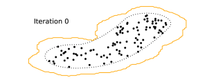
Nested sampling (Skilling2004, ) is a global parameter space exploration algorithm, which zooms in from the entire volume towards the best-fit models by steadily increasing the likelihood threshold. In the process it produces parameter posterior probability distributions and computes the integral over the parameter space. Assume that the parameter space is a $k$-dimensional cube. A number of live points $N_{{\rm live}}$ are randomly placed in the parameter space. Their likelihood is evaluated. Each point represents $1/N_{{\rm live}}$ of the entire volume. The live point with the lowest likelihood $L_{{\rm min}}$ is then removed, implying the removal of space with likelihood below $L_{{\rm min}}$ and shrinkage of the volume to $1-\exp\left(-1/N_{{\rm live}}\right)$, on average. A new random live point is drawn, with the requirement that its likelihood must be above $L_{{\rm min}}$. This replacement procedure is iterated, shrinking the volume exponentially. Each removed (“dead”) point and its likelihood $L_{i}$ is stored. The integral over the parameter space can then be approximated by $Z=\sum_{i}L_{i}\times w_{i}$, where $w_{i}$ is the removed volume at the iteration. At a late stage in the algorithm the volume probed is tiny and the likelihood $L_{i}$ increase is negligible, so that the weights $L_{i}\times w_{i}$ of the remaining live points becomes small. Then the iterative procedure can be stopped (the algorithm converged). The posterior probability distribution of the parameters is approximated as importance samples of weight $L_{i}\times w_{i}$ at the dead point locations, and can be resampled into a set of points with equal weights, for posterior analyses similar to those with Markov Chains. More details on the convergence and error estimates can be found in (skilling2009nested, ).

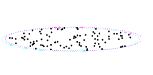
Efficient general solutions exist for drawing a new point above a likelihood threshold in low dimensions ($n_{{\rm dim}}<20$). The idea is to draw only in the neighbourhood of the current live points, which already fulfill the likelihood threshold. The best-known algorithm in astrophysics and cosmology is multinest (Shaw2007, ; Feroz2009, ). There, the contours traced out by the points are clustered into ellipses, and new points drawn from the ellipses. To avoid accidentally cutting away too much of the parameter space, the tightest-fitting ellipses are enlarged by an empirical (problem-specific) factor. Another algorithm is RadFriends (buchner2014statistical, ), which defines the neighbourhood as all points within a radius $r$ of an existing live point. By leaving out randomly a portion of the live points, and determining their distance to the remaining live points, the largest nearest-neighbour radius $r$ is determined. The worst-case analysis through bootstrapping cross-validation over multiple rounds makes RadFriends robust, independent of contour shapes and free of tuning parameters. Figure 1 illustrates the generated regions. RadFriends is efficient if one chooses a standardised euclidean metric (i.e. normalise by the standard deviation of the live points along each axis). The extension to nested sampling proposed in this paper works with any constrained drawing method.

2.2 Simplified description of the idea

Consider two independent nested sampling runs on different data sets, but initialised to the same random number generator state. Initially points are generated from across the entire parameter space, typically giving bad fits. If the data sets are somewhat similar, the phase of zooming to the relevant parameter space will be the same for the two runs. Importantly, while the exact likelihood value will be different for the same point, the ordering of the points will be similar. In other words, for both, the worst-fitting point to be removed is likely the same. The next key insight is that new points can be drawn efficiently from a contour which is the union of the likelihood contours from both runs. Ideally, the point can be accepted by both runs, keeping the runs similar (black points in Figure 2). When a point is shared, the (slow) predicting model has to be only evaluated once, speeding up the run. The model prediction is then compared against the data to produce a likelihood for each data set, an operation which I presume to be fast, e.g., when computing

$${\cal L}_{j}=-\sum_{i}(x_{ij}-m_{i})^{2}/(2\sigma_{ij}^{2})$$ (1)

where $m_{i}$, $x_{ij}$ and $\sigma_{ij}$ are the predictions, measurements and errors in data space respectively for data set $j$.

Figure 2: The analysis of two similar data sets yields at the same iteration similar likelihood contours (the two dotted ellipses). In the presented algorithm a large fraction of live points are shared across data sets (black points), which reduces the number of model evaluations. The differences (cyan crosses and magenta pluses) requiring additional draws.

What if the point can be accepted by only one run? It cannot simply be rejected or accepted in both, otherwise the uniform sampling property of nested sampling is broken. Instead, accepted points are stored in queues, one for each run/data set. Once both runs have a non-empty queue, the first accepted point is removed from each queue and replaces the dead point of each data set. Joint sampling also helps even if a point is not useful right away. If a point was only accepted by run A, but the following point is accepted by both runs, the second point becomes a live point immediately for run B, but can later also become a live point for run A (if it suffices the likelihood threshold at that later iteration). This technique allows sustained sharing of points, decreasing the number of unique live points and increasing the speed-up.

At a later point in the algorithm, the contours may significantly diverge and not share any live points. This is because the best-fit parameters of data sets will differ. Then, nested sampling runs can continue as in the classic case, without speed-up, falling back to a linear scaling. This happens earlier, the more different the data sets are. The run is longer for data sets with high signal-to-noise, making the algorithm most efficient when most observations are near the detection limit. This is typically the case in surveys as a consequence of powerlaw distributions.

2.3 Collaborative nested sampling

I now describe the collaborative nested sampling algorithm. A proof-of-concept reference implementation is available at https://github.com/JohannesBuchner/massivedatans/. The algorithm components are the nested sampling integrator, the constrained sampler and the likelihood function, as in classic nested sampling, except that works on $N$ data sets simultaneously, with $N$ a large number. The constrained sampler behaves substantially different in this algorithm.

2.3.1 Likelihood Function

The likelihood function receives a single parameter vector, and information which data sets to consider. It calls the physical model with the parameter vector to compute into a prediction into data space. The physical model may perform complex and slow numerical computations/simulations at this point. Finally the prediction is compared with the individual data sets to produce a likelihood for each considered data set. The likelihood at this point can be Gaussian (eq. 1), Poisson, a red noise process, or any other probability distribution appropriate for the instrument. In any case, this computation must be fast compared with producing the model predictions to receive any performance gains.

2.3.2 Nested Sampling Integrator

The integrator deals with each run individually just as in standard nested sampling. It keeps track of the remaining volume at the current iteration, and storing the live points and their weights for each data set individually. It calls the constrained sampler (see below), which holds the live points, to receive the next dead point (for all data sets simultaneously). The integrator must also test for convergence, and advance further only those runs which have not yet converged. Here I use the standard criterion that the nested sampling error is $\delta Z<0.5$ (from last equation in skilling2009nested, ). Once all runs have terminated, corresponding to each data set the integral estimates $Z$ and posterior samples are returned, giving the user the same output as e.g., a multinest analysis.

2.3.3 Constrained Sampler

Figure 3: To replace the least likely live point, new points are sampled and placed in queues if they have a high enough likelihood. Once every data set has a non-empty queue, the lowest points are pushed out and stored as dead points by the integrator. In this illustration, $N=4$ data sets are sampled with $N_{{\rm live}}=10$ live points.

The sampler initially draws $N_{{\rm live}}$ live points and stores their likelihoods in an array of size $N\times N_{{\rm live}}$. Sequential IDs are assigned to live points and the mapping between live point IDs and data sets ($N\times N_{{\rm live}}$ indices) is stored. The integrator informs the sampler when it should remove the lowest likelihood point and replace it. The integrator also informs the sampler when some data sets have finished and can be discarded from further consideration, in which case the sampler works as if they had never participated.

The main task of the constrained sampler is to do joint draws under likelihood constraint $L>L_{{\rm min}}$ to replace the lowest likelihood point in each of the $d$ data sets. For this, $d$ initially empty queues are introduced (see Figure 3). First, it is attempted to draw from the joint contour over all data sets (superset draw), i.e. letting RadFriends define a region based on the all unique live points. From this region a point is drawn which has $L>L_{{\rm min}}$ for at least one data set. Some will accept and the corresponding queues are filled. If this fails to fill all queues after several (e.g. 10) attempts, a focussed draw is done. In that case, only the data sets with empty queues are considered, the region is constructed from their live points, and the likelihood only evaluated for these data sets. For example, in the illustration of Figure 3, only Data Set 3 would be considered. Once all queues have at least one entry, nested sampling can advance: For each data set, the first queue entry is removed and replaces the dead live point. In Figure 3 this is illustrated by the queues pushing out the lowest live points. These dead points are returned to the integrator.

Storing queue entries is only useful if they can replace live points in future nested sampling iterations. To be accepted into the queue at position $j$, it must have a likelihood higher than $j$ points from the runs live points and existing entries of the queue. In other words, the first entry must merely beat a single existing live point, the second entry must beat both a live point and either another live point or the first queue entry (which will become a live point in the next iteration).

2.3.4 Data Set Clustering

Figure 4: Association of live point objects with data sets. In this illustration, some live points are shared between the group of Data Sets 1, 2 and 3; these form a connected subgraph. Data Set 4 has separate live points and can be treated independently. In this illustration, $N_{\mathrm{live}}=8$ and $N=4$, but there are only $26$ unique live points.

It can occur that between two groups of data sets the live points are not shared any more, i.e. the live point sets are disjoint (see Figure 4). For example, one may have a dichotomy between broad and narrow line objects, and the contours identify some of the data sets in the former, some in the latter class. Distinct groups caused by diverging likelihood contours are interesting aspect of the exploration: It defines a data set similarity through the constraints in parameter space, based on the likelihood ordering unique to nested sampling. This is different to clustering data sets in data space, which can be non-trivial for varying errors and completeness, and clustering in parameter space could scale poorly with model dimensionality. In practice, diverging live points groups can be identified by finding connected subsets in a graph. As illustrated in Figure 4, the necessary graph can be constructed with nodes corresponding to the data sets, nodes corresponding to the live points, and connecting the graph according to the current live point statuses. Algorithms for identifying connected subsets of graphs are well-known. These data-set groups can be processed independently, avoiding multi-modal contours. In the numerical examples shown in this work, this however does not yield substantial speed-ups.

3 Toy Application: Single-line fitting

Figure 5: Simulated noisy data. The location, width and amplitude of a single line is sought in Gaussian noise for the illustrative problem. The true line locations of the four spectra are indicated by triangles. The cyan data set shows a random fluctuation at $700{\rm nm}$.

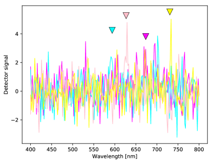
A simple toy example problem illustrates the use and scaling of the algorithm. Lets consider a spectroscopic survey which collected $N$ spectra in the $400-800{\rm nm}$ wavelength range. We look for a Gaussian line at $654{\rm nm}$ rest frame (but randomly shifted) with standard deviation of $0.5{\rm nm}$. The amplitudes vary with a powerlaw distribution with index $3$, with a signal-to-noise ratio of at least two. I generate a large random data set and analyse the first $N$ data sets simultaneously to understand the scaling of the algorithm, with $N=1$ to $N=10^{4}$. Figure 5 presents some high and low signal-to-noise examples of the simulated data set.

The parameter space of the analysis has three dimensions: The amplitude, width and location of a single Gaussian line, with log-uniform/log-uniform/uniform priors from $10^{0-2}$, $0.15-15{\rm nm}$ and $600-1000{\rm nm}$ respectively. The Gaussian line is our “slow-to-compute” physical model. The likelihood function is as in equation 1. A more elaborate example would include physical modelling of an ionised outflow emitting multiple lines with Doppler broadening and red detector noise, without necessitating any modification of the presented algorithm.

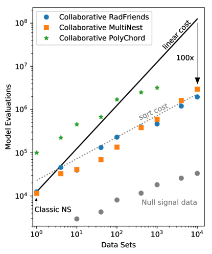
Figure 6 shows the number of model evaluations necessary for analysing $N$ data sets. We implemented our nested sampling variant on top of three constrained drawing methods, RadFriends (buchner2014statistical, ), multi-ellipsoidal sampling (MultiNest, (Shaw2007, ; Feroz2009, )) and eigenvector slice sampling (PolyChord, Handley2015a, , here for simplicity implemented without clustering). The black line shows the baseline linear scaling $O(N)$, i.e. analysing the data sets individually one-by-one. The algorithm scales much better, close to $O(\sqrt{N})$. For instance, it takes only $100$ times more model evaluations to analyse $10,000$ observations than a single observations, a $100$-fold speedup.

Figure 6: Number of model evaluations of collaborative nested sampling applied to RadFriends, multi-ellipsoidal sampling (MultiNest) and whitened slice sampling (PolyChord). A naive approach of independent nested sampling analyses would have a linear scaling (black line). The algorithm scales substantially better, similar to $O(\sqrt{N})$ in the considered problem, giving a 100x speed-up when analysing 10,000 data sets. Analysing Monte Carlo simulated data without signal (gray points) is also faster.

Figure 7: Parameter posterior constraints. Each error bar shows a simulated data set; the four examples from Figure 5 are shown in the same colours. The pink and yellow data sets have been well-detected and characterized, while the magenta line has larger uncertainties. The cyan constraints cover two solutions (see Figure 5). Error bars are centred at the median of the posteriors with the line lengths reflecting the 1-sigma equivalent quantiles.

Figure 8: Line location distribution for objects where the line was well-constrained (blue) compared to the input distribution (black).

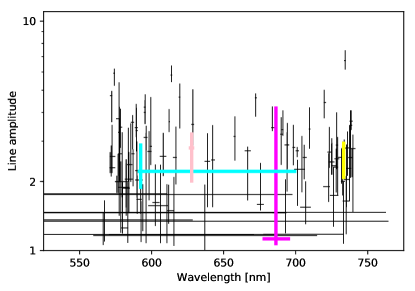
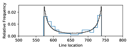
We can now plot the posterior distributions of the found line locations. Figure 7 demonstrates the wide variety of uncertainties. The spectra of Figure 5 are shown in the same colours. For many, the line could be identified and characterised with small uncertainties (yellow, pink, black), for others, the method remains unsure (cyan, magenta). Figure 8 shows that the input redshift distribution is correctly recovered.

Figure 9: Bayes factors between the single-line model and a no-line model. The black histogram shows Bayes factors from analysing the test data set. The red histogram shows Bayes factors from noise-only data. Because the latter has very few values above $B\gtrapprox 10$, a line can be claimed detected beyond that threshold with a low false positive fraction.

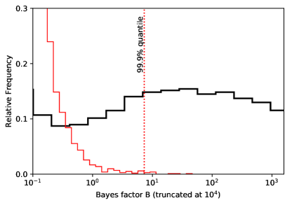
After parameter estimation we can consider model comparison: is the line significantly detected? For this, lets consider the Bayes factor, $B=Z_{1}/Z_{0}$, where $Z_{1}$ is the integral computed by nested sampling under the single-line model, and $Z_{0}$ is the same for the null hypothesis (no line). The latter can be analytically computed as $\ln Z_{0}=-\frac{1}{2}\left[\sum(x_{i}/\sigma_{i})^{2}+\ln 2\pi\sigma_{i}^{2}\right]$. Figure 9 shows in black the derived Bayes factors. To define a lower threshold for significant detections, I Monte Carlo simulate a dataset with $N=10^{4}$ spectra without signal, and derive $Z_{1}$ values. This can be done rapidly with the presented algorithm. The red histogram in Figure 9 shows the resulting Bayes factors. The $99.9\%$ quantile of $B$-values in this signal-free data set is $B\approx 10$. Therefore, in the “real” data, those with a Bayes factor $B>10$ can be securely claimed to have a line, with a small fraction of false detection ($p<0.001$).

4 Application to Imaging Spectroscopy

Figure 10: MUSE IFU data analysed with Collaborative Nested Sampling. Top left panel: White image of the input data. Several blobs and a extended arc is visible. Top right panel: Bayes factor $B$ comparing the single-stellar population model to a no-signal model. In the arc and blobs, $\log B>0$. The remaining panels present posterior parameters (left) and uncertainties (right). Redshift $z$ is well-constrained across the arc ($z\approx 0.6$) and the closer blobs ($z\approx 0.4$). While the blobs had a brief star formation episode ($\log\tau/\mathrm{yr}\approx 7$) long ago (age > $10^{10}$ years), the arc shows evidence for recent star formation (younger age, slower decay $\tau$).

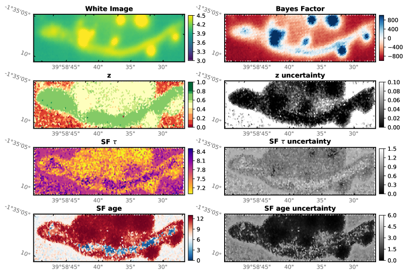
Finally, I apply collaborative nested sampling to a real-world data set. Integral-field unit (IFU) observations, where many spectra are taken in proximity on the sky are ideal for applying the algorithm. The MUSE spectrograph (1arcmin² field of view, wavelength range 480-930nm; (Bacon2010, )) observed the Abell 370 galaxy cluster in November 2014 (PI: Richard) for one hour. Following e.g., (Lagattuta2017, ) and (Patricio2018, ), standard data reduction procedures and sky line subtraction ((Soto2016ZAP, )) were used, and the errors increased by 20% of the data value to account for model inaccuracies. The chosen region in the sky (A370-sys1 in (Patricio2018, )) includes several galaxies, some of which heavily distorted by strong lensing. Its white image (sum across the spectrum) is shown in the top-left panel of Figure 10. The 169 arcsec² sized region is covered by 4223 fibers, each of which providing a spectrum with measured intensity and error.

A simple stellar population is used to model the spectra. The classic Bruzual & Charlot model stellar spectra (Bruzual2003, ) are weighed by an exponential star formation (decay timescale $\tau$) at time $t$ Gyrs in the past. Additionally, dust extinction is allowed through a Calzetti law(Calzetti2000, ) and the model is redshifted. To avoid a degeneracy with star formation age, I assume solar metallicity. This model thus has four parameters: redshift $z$ (0-1), star formation age $t$ (0-13 Gyr), star formation decay time $\tau$ ($10^{6-9}$ Gyr) and extinction $E(B-V)$ (0-1). Uniform priors are applied on $z$, $t$, $\log\tau$ and $E(B-V)$.

A Gaussian likelihood compares the model spectrum $M_{i}$ against the measurements $\mu_{i}$ and errors $\sigma_{i}$. To avoid having the model normalisation $s$ as a fitting parameter, it is marginalised over, by setting

$$s=\sum_{i}\left(\mu_{i}M_{i}\sigma_{i}^{-2}\right)/\sum_{i}\left(M_{i}^{2}\sigma_{i}^{-2}\right)$$ (2)

and neglecting constants in the likelihood (see (Arnouts1999, ) for more details):

$$\log L=-\frac{1}{2}\sum\left[(\mu_{i}-s\cdot M_{i})/\sigma_{i}\right]^{2}$$ (3)

With the model, likelihood and data defined, I apply collaborative nested sampling with multi-ellipsoidal sampling and derive posterior parameter distribution at each spaxel. Evidence values are also obtained. Similar to the previous section, Bayes factors are computed and shown in the top right panel in Figure 10 at each spaxel. The red areas indicate where the data prefer no input signal over the stellar model.

The second row of Figure 10 shows the derived redshift. Uncertainties (right panel) are extremely small (typically 0.001) over most of the image. Two solutions are visible in the left panel: The arc (green) is at distinctly higher redshifts than the blobs (yellow). Extended emission at the same redshift as the blobs is detected.

The third and forth row present the star formation properties in each pixel. The arc shows evidence for recent star formation. While uncertainties on the decay parameter are not small, generally the arc has a longer ($10^{8}\,\mathrm{Gyr}$) star formation episode than the blobs ($10^{7}\,\mathrm{Gyr}$). The extinction is constant over image and shows small values ($<0.1$; not shown). The model used here is overly simple and I do not interpret the physical meaning in great detail (see (Patricio2018, ) instead). In particular, the relation between metallicity and age should be explored further. (Patricio2018, ) however derived similar values e.g., for the star formation age and timescale when considering the stacked spectrum across the entire arc.

This application demonstrates the usefulness of collaborative nested sampling in a realistic dataset. Physical parameters were extracted while exploiting that spatial neighbours have similar physical properties. However, no assumption about smoothness or neighbourhood was made, i.e., the constraints at each pixel are independent. Also note that in every pixel, a posterior distribution over the parameters is derived. Here, the collaborative nested sampling analysis of 4223 fibers required 14.4 million likelihood evaluations (140h). This corresponds to a quadrupling of the efficiency compared to analysing only 100 fibers, which required 2.8 million likelihood evaluations (14.9h).

5 Discussion

Collaborative nested sampling is a scalable algorithm suitable for analysing massive data sets with arbitrarily complex physical models and complex, inhomogeneous noise properties. The algorithm brings to the Big Data regime parameter estimation with uncertainties, classification of objects and distinction between physical processes.

The key insight in this work is to take advantage of a property specific to nested sampling: The sampling regions can look similar across similar data sets, and rejection sampling from the union of contours is permitted. Collaborative nested sampling reduces the number of unique model evaluations, in particular at the beginning of the nested sampling run. The same approach cannot be followed with Markov Chain proposals: There, the proposal depends on the current point, and deviating acceptances prohibit a later joint proposal.

Compared to embarrassingly parallel analyses, collaborative nested sampling excels in specific types of problems, which have many uncertain data sets of similar structure into which a slow physical model is predicting. The algorithm has some overhead related to the management of live points, in particularly to determine the unique set of live points across a dynamically selected subgroup of data sets. The memory usage also grows if big data sets have to be held in the same machine. If only chunks of $N$ are managable, the analyses can be split into such sizes and analysed in parallel across multiple machines. In that case, one can take advantage of the scaling of the algorithm until $N$.

The algorithm can be applied immediately to any existing large data sets. Compared to other Big Data analysis approaches, nested sampling supports model comparison and yields full probability distributions on arbitrary models, allowing the exploration of degenerate fit solutions. Furthermore, the instrument response can be modelled out and separated from the process of interest. To give one application example, eROSITA (Predehl2014eRosita, ) requires the source classification and characterisation of 3 million point sources in its all-sky X-ray survey (Kolodzig2012, ). The position-dependent detector response and non-Gaussianity of count data make standard machine learning approaches difficult to apply.

Even in the analysis of single objects the presented algorithm can help. One might test the correctness of selecting a more complex model, e.g., based on Bayes factors, as in the toy example presented. Large Monte Carlo simulations of a null hypothesis model can be quickly analysed with the presented method, with a model evaluation cost that is essentially independent of the number of generated data sets. G̊oing further, approaches to validate models and Bayesian inference \cite[citep]{(e.g., \@@bibref{AuthorsPhrase1Year}{Talts2018}{\@@citephrase{, }}{})} over the entire parameter space can be sped up.

6 Acknowledgements

I thank Surangkhana Rukdee and Frederik Beaujean for reading the manuscript, and Franz E. Bauer for help with MUSE data. This work made use of the nestle free software implementation of the MultiNest algorithm and the matplotlib plotting library (matplotlib, ). I thank the two anonymous referees for helpful comments and suggestions.

I acknowledge support from the CONICYT-Chile grants Basal-CATA PFB-06/2007, FONDECYT Postdoctorados 3160439 and the Ministry of Economy, Development, and Tourism’s Millennium Science Initiative through grant IC120009, awarded to The Millennium Institute of Astrophysics, MAS. This research was supported by the DFG cluster of excellence “Origin and Structure of the Universe”.

References

- (1) Arnouts, S., Cristiani, S., Moscardini, L., Matarrese, S., Lucchin, F., Fontana, A., Giallongo, E.: Measuring and modelling the redshift evolution of clustering: the Hubble Deep Field North. MNRAS310, 540–556 (1999). DOI 10.1046/j.1365-8711.1999.02978.x
- (2) Bacon, R., Accardo, M., Adjali, L., Anwand, H., Bauer, S., Biswas, I., Blaizot, J., Boudon, D., Brau-Nogue, S., Brinchmann, J., Caillier, P., Capoani, L., Carollo, C.M., Contini, T., Couderc, P., Daguisé, E., Deiries, S., Delabre, B., Dreizler, S., Dubois, J., Dupieux, M., Dupuy, C., Emsellem, E., Fechner, T., Fleischmann, A., François, M., Gallou, G., Gharsa, T., Glindemann, A., Gojak, D., Guiderdoni, B., Hansali, G., Hahn, T., Jarno, A., Kelz, A., Koehler, C., Kosmalski, J., Laurent, F., Le Floch, M., Lilly, S.J., Lizon, J.L., Loupias, M., Manescau, A., Monstein, C., Nicklas, H., Olaya, J.C., Pares, L., Pasquini, L., Pécontal-Rousset, A., Pelló, R., Petit, C., Popow, E., Reiss, R., Remillieux, A., Renault, E., Roth, M., Rupprecht, G., Serre, D., Schaye, J., Soucail, G., Steinmetz, M., Streicher, O., Stuik, R., Valentin, H., Vernet, J., Weilbacher, P., Wisotzki, L., Yerle, N.: The MUSE second-generation VLT instrument. In: Ground-based and Airborne Instrumentation for Astronomy III, SPIE, vol. 7735, p. 773508 (2010). DOI 10.1117/12.856027
- (3) Bruzual, G., Charlot, S.: Stellar population synthesis at the resolution of 2003. MNRAS344, 1000–1028 (2003). DOI 10.1046/j.1365-8711.2003.06897.x
- (4) Buchner, J.: A statistical test for nested sampling algorithms. Statistics and Computing pp. 1–10 (2014)
- (5) Calzetti, D., Armus, L., Bohlin, R.C., Kinney, A.L., Koornneef, J., Storchi-Bergmann, T.: The Dust Content and Opacity of Actively Star-forming Galaxies. ApJL533, 682–695 (2000). DOI 10.1086/308692
- (6) Feigelson, E.D., Babu, G.J.: Big data in astronomy. Significance 9(4), 22–25 (2012). DOI 10.1111/j.1740-9713.2012.00587.x. URL http://dx.doi.org/10.1111/j.1740-9713.2012.00587.x
- (7) Feroz, F., Hobson, M.P., Bridges, M.: MULTINEST: an efficient and robust Bayesian inference tool for cosmology and particle physics. MNRAS398, 1601–1614 (2009). DOI 10.1111/j.1365-2966.2009.14548.x
- (8) Handley, W.J., Hobson, M.P., Lasenby, A.N.: POLYCHORD: next-generation nested sampling. MNRAS453, 4384–4398 (2015). DOI 10.1093/mnras/stv1911
- (9) Hunter, J.D.: Matplotlib: A 2d graphics environment. Computing In Science & Engineering 9(3), 90–95 (2007)
- (10) Kolodzig, A., Gilfanov, M., Sunyaev, R., Sazonov, S., Brusa, M.: AGN and QSOs in the eROSITA All-Sky Survey. I. Statistical properties. A&A558, A89 (2013). DOI 10.1051/0004-6361/201220880
- (11) Kremer, J., Stensbo-Smidt, K., Gieseke, F., Steenstrup Pedersen, K., Igel, C.: Big Universe, Big Data: Machine Learning and Image Analysis for Astronomy. ArXiv e-prints (2017)
- (12) Lagattuta, D.J., Richard, J., Clément, B., Mahler, G., Patrício, V., Pelló, R., Soucail, G., Schmidt, K.B., Wisotzki, L., Martinez, J., Bina, D.: Lens modelling Abell 370: crowning the final frontier field with MUSE. MNRAS469, 3946–3964 (2017). DOI 10.1093/mnras/stx1079
- (13) Mickaelian, A.M.: Astronomical surveys and big data. Baltic Astronomy 25, 75–88 (2016)
- (14) Patrício, V., Richard, J., Carton, D., Contini, T., Epinat, B., Brinchmann, J., Schmidt, K.B., Krajnović, D., Bouché, N., Weilbacher, P.M., Pelló, R., Caruana, J., Maseda, M., Finley, H., Bauer, F.E., Martinez, J., Mahler, G., Lagattuta, D., Clément, B., Soucail, G., Wisotzki, L.: Kinematics, turbulence, and star formation of z 1 strongly lensed galaxies seen with MUSE. MNRAS477, 18–44 (2018). DOI 10.1093/mnras/sty555
- (15) Predehl, P., Andritschke, R., Becker, W., Bornemann, W., Bräuninger, H., Brunner, H., Boller, T., Burwitz, V., Burkert, W., Clerc, N., Churazov, E., Coutinho, D., Dennerl, K., Eder, J., Emberger, V., Eraerds, T., Freyberg, M.J., Friedrich, P., Fürmetz, M., Georgakakis, A., Grossberger, C., Haberl, F., Hälker, O., Hartner, G., Hasinger, G., Hoelzl, J., Huber, H., von Kienlin, A., Kink, W., Kreykenbohm, I., Lamer, G., Lomakin, I., Lapchov, I., Lovisari, L., Meidinger, N., Merloni, A., Mican, B., Mohr, J., Müller, S., Nandra, K., Pacaud, F., Pavlinsky, M.N., Perinati, E., Pfeffermann, E., Pietschner, D., Reiffers, J., Reiprich, T., Robrade, J., Salvato, M., Santangelo, A.E., Sasaki, M., Scheuerle, H., Schmid, C., Schmitt, J., Schwope, A.D., Sunyaev, R., Tenzer, C., Tiedemann, L., Xu, W., Yaroshenko, V., Walther, S., Wille, M., Wilms, J., Zhang, Y.Y.: eROSITA on SRG. In: Society of Photo-Optical Instrumentation Engineers (SPIE) Conference Series, Society of Photo-Optical Instrumentation Engineers (SPIE) Conference Series, vol. 9144, p. 1 (2014). DOI 10.1117/12.2055426. URL http://proceedings.spiedigitallibrary.org/pdfaccess.ashx?ResourceID=7241319&PDFSource=24
- (16) Shaw, J.R., Bridges, M., Hobson, M.P.: Efficient Bayesian inference for multimodal problems in cosmology. MNRAS378, 1365–1370 (2007). DOI 10.1111/j.1365-2966.2007.11871.x
- (17) Skilling, J.: Nested sampling. In: AIP Conference Proceedings, vol. 735, p. 395 (2004). URL http://proceedings.aip.org/resource/2/apcpcs/735/1/395_1
- (18) Skilling, J.: Nested sampling’s convergence. In: BAYESIAN INFERENCE AND MAXIMUM ENTROPY METHODS IN SCIENCE AND ENGINEERING: The 29th International Workshop on Bayesian Inference and Maximum Entropy Methods in Science and Engineering, vol. 1193, pp. 277–291. AIP Publishing (2009). URL http://scitation.aip.org/content/aip/proceeding/aipcp/10.1063/1.3275625
- (19) Soto, K.T., Lilly, S.J., Bacon, R., Richard, J., Conseil, S.: ZAP - enhanced PCA sky subtraction for integral field spectroscopy. MNRAS458, 3210–3220 (2016). DOI 10.1093/mnras/stw474
- (20) Talts, S., Betancourt, M., Simpson, D., Vehtari, A., Gelman, A.: Validating Bayesian Inference Algorithms with Simulation-Based Calibration. ArXiv e-prints (2018)
- (21) Zhang, Y., Zhao, Y.: Astronomy in the big data era. Data Science Journal 14 (2015)