On the foundations of general relativistic celestial mechanics

Abstract

Towards the end of nineteenth century, Celestial Mechanics provided the most powerful tools to test Newtonian gravity in the solar systems, and led also to the discovery of chaos in modern science. Nowadays, in light of general relativity, Celestial Mechanics leads to a new perspective on the motion of satellites and planets. The reader is here introduced to the modern formulation of the problem of motion, following what the leaders in the field have been teaching since the nineties. In particular, the use of a global chart for the overall dynamics of $N$ bodies and $N$ local charts describing the internal dynamics of each body. The next logical step studies in detail how to split the $N$-body problem into two sub-problems concerning the internal and external dynamics, how to achieve the effacement properties that would allow a decoupling of the two sub-problems, how to define external-potential-effacing coordinates and how to generalize the Newtonian multipole and tidal moments. The review paper ends with an assessment of the nonlocal equations of motion obtained within such a framework, a description of the modifications induced by general relativity on the theoretical analysis of the Newtonian three-body problem, and a mention of the potentialities of the analysis of solar-system metric data carried out with the Planetary Ephemeris Program.

I Introduction

At the end of the nineteenth century, two hundred years after the publication of Newton’s Principia, Celestial Mechanics was a very successful branch of Mechanics (with hindsight, we would speak of Classical Mechanics, but the Planck constant had not yet been postulated nor measured). The monumental treatise by Tisserand T1 ; T2 ; T3 ; T4 had studied thoroughly planetary motions and their perturbations T1 , rotational motion of celestial bodies T2 , theories of lunar motion T3 , the theories of Jupiter and Saturn satellites T4 , and perturbations of small planets T4 . Moreover, in his outstanding work on new methods in celestial mechanics P1 ; P2 ; P3 ; P4 , Poincaré discovered periodic solutions of the three-body problem P2 ; P4 , asymptotic P2 and doubly asymptotic solutions P4 , the nonexistence of uniform integrals P2 , the theory of integral invariants P4 , and the whole topic of chaos became part of modern science, jointly with an assessment of asymptotic methods for studying secular terms P3 in the equations of celestial mechanics, gaining a better understanding of the limitations of several methods used by astronomers and applied mathematicians.

However, as was stressed by Poincaré in the introduction P2 to volume 1 of his monumental treatise, the relevance of celestial mechanics from the point of view of fundamental physics lies mainly in the possibility of using it to ascertain whether Newton’s theory provides the best theory of gravity at all scales (i.e. within the solar system and far beyond that). Although mankind landed safely on the moon thanks to Newtonian celestial mechanics in Szebehely’s book Sze , the discovery of general relativity led to a novel perspective on the classical problems of Newtonian celestial mechanics, as is clear from the work of Lorenz and Droste Lor , Einstein et al. E1 ; E2 , Levi-Civita Levi-Civita , Fock Fock1959 , Brumberg BR1 , Kopeikin K1 , Yamada et al. Y1 . But the most systematic application of general relativity methods to celestial mechanics is due to Damour and his collaborators D1987 ; BD ; D1 ; D2 ; D3 ; D4 (cf. Ref. ALBA1 ).

In our review paper, aimed at helping the general reader to become familiar with the modern formulation of the problem of motion, Sec. II is devoted to the theory of reference systems, Sec. III studies Newtonian tidal and multipole expansions, Sec. IV leads to relativistic tidal and multipole expansions, and the monopole model is briefly reviewed in Sec. V. Last, the integro-differential dynamical equations are discussed in Sec. VI and the effects of general relativity on the restricted three-body problem are summarized in Sec. VII; Sec. VIII outlines the potentialities of the analysis of solar-system metric data carried out with the Planetary Ephemeris Program, while concluding remarks are presented in Sec. IX.

II Theory of reference systems

We here outline the formalism lying behind general relativistic celestial mechanics of systems of $N$ arbitrarily composed and shaped, weakly self-gravitating, rotating, deformable bodies (D1, ; D2, ; D3, ; D4, ). Such a framework yields a complete description, at the first post-Newtonian order, of both the global dynamics of the $N$-body system and of the local structure of each body by employing $N+1$ coordinate charts: one global chart $x^{\mu}\equiv(ct,x^{i})$ $(i=1,2,3)$ covering the entire manifold $V_{4}$ (see below) for the overall dynamics of the $N$ bodies and $N$ local charts $X^{\alpha}_{\,A}\equiv(cT_{A},X^{a}_{A})$ $(A=1,2,\dots,N)$, $(a=1,2,3)$ describing the internal dynamics of each body. Hereafter, inspired by Refs. (D1, ; D2, ; D3, ; D4, ), we will use the following conventions: the $N$ bodies are labelled by upper case Latin indices $A,B,C=1,2,\dots,N$; the global coordinates $x^{\mu}\equiv(ct,x^{i})$ are such that spacetime indices belong to the second part of Greek alphabet $(\mu,\nu,\lambda,\dots)$ while purely space indices follow the second part of the Latin alphabet $(i,j,k,\dots)$; the local coordinate systems $X^{\alpha}_{\,A}\equiv(cT_{A},X^{a}_{A})$ are such that spacetime indices and spatial indices are taken from the first part of the Greek and Latin alphabet, respectively. In order to ease the notation, sometimes the labels $A,B,C$ are omitted. The essential ingredient of the formalism is represented by the exponential parametrization (in all frames) of the metric tensor which leads to the linearization of both the field equations (expressible in terms of some potential functions, in strict analogy with Maxwell theory of electromagnetism) and the transformation laws under a change of reference system.

Let there be given a four-dimensional smooth differentiable abstract manifold $V_{4}$ endowed with $N$ abstract world lines $\mathfrak{L}_{A}$ $(A=1,2,\dots,N)$ and $N$ topological tubes $\mathcal{T}_{A}\subset V_{4}$ representing some open neighbourhood of $\mathfrak{L}_{A}$. The local chart $X^{\alpha}_{\,A}$ is said to be adapted to the world line if it maps every point $P$ belonging to $\mathfrak{L}_{A}$ onto the “time axis” of $\mathbb{R}^{4}$, i.e.,

$$X^{\alpha}_{\,A}:\mathcal{T}_{A}\rightarrow\mathbb{R}^{4}\;|\;X^{\alpha}_{\,A}(P)=(S,0,0,0),\;\;P\in\mathfrak{L}_{A},\;S\in\mathbb{R}.$$ (1)

In this way it is possible to parametrize $\mathfrak{L}_{A}$ through the real factor $S=cT$ which fulfils the role of a special affine parameter having the physical dimensions of a length, i.e., $X^{\alpha}_{\,A}(P(S))=(S,0,0,0),\;(S\in\mathbb{R},\;P\in\mathfrak{L}_{A})$. Moreover, we can define a one-parameter family of vectorial bases $\boldsymbol{{\rm e}}^{A}_{\alpha}(S)$ along $\mathfrak{L}_{A}$ (i.e., a basis of the tangent vector space $T_{P(S)}V_{4}$ to $V_{4}$ at $P(S)\in\mathfrak{L}_{A}$) as

$$\boldsymbol{{\rm e}}^{A}_{\alpha}(S)=\left.\dfrac{\partial}{\partial X^{\alpha}_{\,A}}\right|_{P(S)},$$ (2)

such that

$$\boldsymbol{{\rm e}}^{A}_{0}(S)=\left.\dfrac{\partial}{\partial S}\right|_{P(S)},$$ (3)

represents the tangent vector to the $S$-parametrized world line.

By means of the metric-independent structure introduced above the most general coordinate transformation linking global and local coordinates D1

$$x^{\mu}=f^{\mu}_{\,A}(X^{0}_{A},X^{1}_{A},X^{2}_{A},X^{3}_{A}),$$ (4)

can be expressed by (label $A$ omitted)

$$x^{\mu}(X^{\alpha})=z^{\mu}(X^{0})+e_{a}^{\;\mu}(X^{0})X^{a}+\xi^{\mu}(X^{0},X^{a}),$$ (5)

where (label $A$ written explicitly)

$$z^{\mu}_{A}(S)=f^{\mu}_{\,A}(S,0,0,0),$$ (6)

represents the expression that the $S$-parametrized world line $\mathfrak{L}_{A}$ assumes in the global coordinate system $x^{\mu}$, while

$$e_{A\,a}^{\;\mu}(S)=\dfrac{\partial f^{\mu}_{\,A}}{\partial X^{a}_{\,A}}(S,0,0,0),$$ (7)

are the global components of the three vectors $\boldsymbol{{\rm e}}^{A}_{a}(S)$ (cf. Eq. (2)) and eventually the term

$$\xi^{\mu}_{\,A}(S,X^{a}_{\,A})=f^{\mu}_{\,A}(S,X^{a}_{\,A})-f^{\mu}_{\,A}(S,\boldsymbol{0})-X^{a}_{\,A}\dfrac{\partial f^{\mu}_{\,A}}{\partial X^{a}_{\,A}}(S,\boldsymbol{0}),$$ (8)

is such that

$$\xi^{\mu}(X^{0},X^{a})={\rm O}\left((X^{a})^{2}\right)\;\;\;{\rm as}\;X^{a}\rightarrow 0\;\;{\rm with\;fixed}\;X^{0}.$$ (9)

In particular, the last condition results from the requirement that the metric admits a post-Newtonian expansion of the usual type (see Eq. (13) below). Note also that Eq. (7) is closely connected with the values of the Jacobian matrix elements

$$A^{\mu}_{\,\alpha}=\dfrac{\partial x^{\mu}(X^{\beta})}{\partial X^{\alpha}},$$ (10)

of the coordinate transformation (4) evaluated at the origin of the local system.

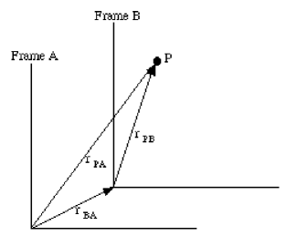
Figure 1: The Newtonian decomposition of a position vector in fixed (A) and mobile (B) coordinate systems.

We believe that Eq. (5) can be better understood once we have compared it with the Newtonian decomposition of a position vector $\mathbb{r}_{{\rm PA}}$ in two frames (Fig. 1)

$$\mathbb{r}_{{\rm PA}}=\mathbb{r}_{{\rm BA}}+\mathbb{r}_{{\rm PB}}.$$ (11)

In fact, since the term $z^{\mu}(X^{0})$ occurring in (5) just describes the world line $\mathfrak{L}_{A}$ in the global frame, it reminds us of the vector $\mathbb{r}_{{\rm BA}}$ denoting the position of the origin of the mobile frame as seen in the fixed one. As a result, in the post-Newtonian pattern the global spatial coordinates of the origin of the local coordinate system, following (the world line of) every body of the system, expressed as functions of the global time $t$ will be represented by $x^{i}=z^{i}(t)$. Moreover, the term $e_{a}^{\;\mu}(X^{0})X^{a}$ appearing in Eq. (5) resembles the quantity $\mathbb{r}_{{\rm PB}}=x_{{\rm PB}}\hat{x}_{{\rm B}}+y_{{\rm PB}}\hat{y}_{{\rm B}}+z_{{\rm PB}}\hat{z}_{{\rm B}}$ ($\hat{x}_{{\rm B}}$, $\hat{y}_{{\rm B}}$, and $\hat{z}_{{\rm B}}$ being the unit vectors of the axes of the mobile system) because, as pointed out before, $e_{a}^{\;\mu}$ are the global version of the vector basis of tangent vector space $T_{P(S)}V_{4}$. Finally the $\xi^{\mu}$ term of (5) measures the deviation between Newtonian and post-Newtonian dynamics. Furthermore, it is essential to stress that the structure of Eq. (5) results from the post-Newtonian analysis of those effacement properties which could allow, like in Newtonian theory, a separation of the $N$-body problem into two decoupled sub-problems: the internal problem concerning the motion of each body around its centre of mass and the external one, involving the dynamics of all centres of mass of the bodies. In fact, in the Newtonian framework the key point towards the achievement of such a decoupling is represented by the existence of some nonrotating accelerated mass-centred-frames with respect to which, in the description of the internal problem, the effects of the external gravitational potential acting locally on each body are suppressed, leaving only small (tidal) effects. The search for a good post-Newtonian definition of some external-gravitational-field-effacing coordinates in the analysis of the $N$-body internal problem has led to Eq. (5) D1987 . This issue is strictly connected to the post-Newtonian definition of center-of-mass frames and will be further discussed later on.

At this stage, we can define a metric structure both in the global frame and in the $N$ local systems by

$$\begin{split}&g_{\mu\nu}(x^{\lambda})=\eta_{\mu\nu}+h_{\mu\nu}(x^{\lambda}),\\ &G^{A}_{\;\alpha\beta}(X^{\gamma})=\eta_{\alpha\beta}+H^{A}_{\;\alpha\beta}(X^{\gamma}),\;\;\;(A=1,2,\dots,N),\end{split}$$ (12)

$\eta_{\mu\nu}$ being the flat Minkowski metric, whereas $h_{\mu\nu}$ and $H^{A}_{\;\alpha\beta}$ represent the metric deviation in the global and in the local frames, respectively. By making the standard post-Newtonian assumptions for the metric ($T\equiv X^{0}/c$) D1 ; D2

$$\begin{split}&h_{00}(t,\mathbb{x})={\rm O}(c^{-2}),\;\;\;\;\;\;\;\;\;\;\;\;\;\;\;\;\;h_{0i}(t,\mathbb{x})={\rm O}(c^{-3}),\;\;\;\;\;\;\;\;\;\;\;\;\;\;\;\;\;h_{ij}(t,\mathbb{x})={\rm O}(c^{-2}),\;\;\;\;\;\;\;\;\;\;\;\;\;\;\;\;\;\\ &H^{A}_{\;00}(T,\mathbb{X})={\rm O}(c^{-2}),\;\;\;\;\;\;\;\;\;\;\;\;\;H^{A}_{\;0a}(T,\mathbb{X})={\rm O}(c^{-3}),\;\;\;\;\;\;\;\;\;\;\;\;\;H^{A}_{\;ab}(T,\mathbb{X})={\rm O}(c^{-2}),\;\;\;\;\;\;\;\;\;\;\;\;\;\;\;\;\;\end{split}$$ (13)

and by postulating that the coordinate transformation (5) involves Jacobian matrix elements having the form (“slow motion assumption”) D1

$$A^{0}_{0}={\rm O}(c^{-0}),\;A^{i}_{0}={\rm O}(c^{-1}),\;A^{0}_{a}={\rm O}(c^{-1}),\;A^{i}_{a}={\rm O}(c^{-0}),\;$$ (14)

the $z-e-\xi$ elements appearing in (5) turn out to be highly constrained D1 ; D2 . In particular, the $3\times 3$ time-dependent matrix $e^{i}_{a}(S)$ is such that

$$\begin{split}&\delta_{ij}\,e^{i}_{a}(S)\,e^{j}_{b}(S)=e^{i}_{a}(S)\,e^{i}_{b}(S)=\delta_{ab}+{\rm O}(c^{-2}),\\ &\dfrac{{\rm d}}{{\rm d}T}e^{i}_{a}(T)={\rm O}(c^{-2}),\end{split}$$ (15)

resembling, modulo ${\rm O}(c^{-2})$ terms, a slowly changing Euclidean rotation matrix. The only quantity occurring in (5) which is not constrained at the first post-Newtonian order by Eqs. (13) and (14) is represented by the term $\xi^{i}$, since it is found in Ref. D1 that $\xi^{i}={\rm O}(c^{-2})$. This peculiarity leaves some (gauge) freedom to the spatial coordinates which can be restricted by imposing in all $N+1$ frames four algebraic conditions called “spatial isotropy conditions” which are represented by (D1, ; D2, ; D3, ; D4, )

$$\begin{split}&-g_{00}g_{ij}=\delta_{ij}+{\rm O}(c^{-4}),\\ &-G^{A}_{\;00}G^{A}_{\;ab}=\delta_{ab}+{\rm O}(c^{-4}),\;\;\;\;\;\;\,\;\forall\;A.\end{split}$$ (16)

The coordinates selected by Eq. (16) are referred to as “conformally Cartesian” or “isotropic”. The gauge choice (16) fixes completely the spatial coordinate freedom in all frames up to time-dependent isometries of Euclidean three-space. In other words, Eq. (16) leaves a gauge freedom in the time coordinate at ${\rm O}(c^{-4})$ in all coordinate systems. Moreover, the spatial isotropy conditions (16) imply that the three spatial coordinates $x^{i}$ are harmonic at the second post-Newtonian order, i.e.,

$$\square_{g}x^{i}={\rm O}(c^{-4}),$$ (17)

$\square_{g}=\left(1/\sqrt{-g}\right)\partial_{\mu}\left(\sqrt{-g}\,g^{\mu\nu}\partial_{\nu}\right)$ being the d’ Alembert wave operator acting on scalar functions. Since Eq. (17) follows directly from the imposition of the (spatial part of the full) standard harmonic and post-Newtonian gauges, we see that (16) encompasses both these choices.

At this stage, by enforcing both the assumptions (13) and (14) and the spatial isotropy conditions (16) the structure of the transformation (5) is further constrained, leaving only the usual Newtonian freedom involving the choice of an arbitrarily moving origin $z^{i}(t)$ of the local frame (we will see that a preferred choice is the one for which the Blanchet-Damour mass dipole vanishes BD ) and of a slowly changing SO$(3)$ rotation matrix $R^{i}_{a}(T)$ describing the rotational state of the local spatial coordinate grid (together with the gauge freedom for time coordinate we have just mentioned). The matrix $R^{i}_{a}(T)$ is defined through the $3\times 3$ matrix $e^{i}_{a}(T)$, since it turns out to be proportional, apart from second-order terms, to the space-space part of a general Lorentz transformation (i.e., a boost combined with an arbitrary rotation matrix) D1

$$\bigg{(}1+{\rm O}\left(c^{-2}\right)\bigg{)}e^{i}_{a}(T)=\left(1+\dfrac{1}{2c^{2}}\mathbb{v}^{2}\right)\left(\delta^{ij}+\dfrac{1}{2c^{2}}v^{i}v^{j}\right)R^{j}_{a}(T)+{\rm O}(c^{-4}),$$ (18)

$b^{ij}=\delta^{ij}+\dfrac{v^{i}v^{j}}{2c^{2}}$ being the boost components with

$$v^{i}=\dfrac{{\rm d}z^{i}}{{\rm d}t}=\dfrac{{\rm d}z^{i}}{{\rm d}T}+{\rm O}(c^{-2}),$$ (19)

representing the velocity of the origin of the local frame. The slow post-Newtonian evolution of $R^{i}_{a}(T)$ is caught by

$$\dfrac{{\rm d}}{{\rm d}T}R^{i}_{a}(T)={\rm O}(c^{-2}),$$ (20)

while its SO$(3)$ structure is enlightened through the relations

$$\begin{split}&R^{i}_{a}(T)\,R^{j}_{a}(T)=\delta^{ij},\\ &R^{i}_{a}(T)\,R^{i}_{b}(T)=\delta_{ab}.\end{split}$$ (21)

At this stage, we can introduce the exponential parametrization of the ten independent unknown metric tensor components through the potential $w_{\mu}=(w,w_{i})$, starting from the global frame D1 ; BD

$$\begin{split}&g_{00}=-{\rm e}^{-2w/c^{2}},\\ &g_{0i}=-4w_{i}/c^{3},\\ &g_{ij}=\gamma_{ij}\,{\rm e}^{2w/c^{2}},\end{split}$$ (22)

$\gamma_{ij}$ being the three-metric associated to $g_{\mu\nu}$ by

$$\gamma_{ij}=-g_{00}g_{ij}+g_{0i}g_{0j}.$$ (23)

By exploiting Eq. (22) and the post-Newtonian assumptions (13), six of the Einstein equations imply that the spatial coordinates are Cartesian coordinates for the three-metric, i.e.,

$$\gamma_{ij}=\delta_{ij}+{\rm O}(c^{-4}),$$ (24)

whereas the four remaining Einstein equations give coupled linear partial differential equations for $w$ and the three-vector components $w^{i}=w_{i}$ expressed by ($\partial_{t}=c\partial_{0}=\partial/\partial t$, $w^{i}\equiv\gamma^{ij}w_{j}$) D1

$$\begin{split}&\square w+\dfrac{4}{c^{2}}\partial_{t}\left(\partial_{t}w+\partial_{i}w_{i}\right)=-4\pi G\sigma+{\rm O}(c^{-4}),\\ &\triangle w_{i}-\partial_{i}\partial_{j}w_{j}-\partial_{t}\partial_{i}w=-4\pi G\sigma_{i}+{\rm O}(c^{-2}),\end{split}$$ (25)

where $-\triangle$ is the flat-space Laplacian (in general we would have $\triangle=\gamma^{ij}D_{j}D_{i}$, $D_{i}$ being the (spatial) covariant derivative associated to $\gamma_{ij}$), while $\sigma$ and $\sigma_{i}$ represent a gravitational mass density and a mass current density, respectively. They are defined in terms of the contravariant components of the (post-Newtonian) stress-energy tensor as

$$\begin{split}&\sigma\equiv\dfrac{T^{00}+T^{jj}}{c^{2}},\\ &\sigma^{i}\equiv\dfrac{T^{0i}}{c}.\end{split}$$ (27)

Note that the definitions given above are independent of the particular form taken by $T^{\mu\nu}$, which is supposed to have a very general structure, being subjected only to conditions (26). Equations (25) are found to be gauge invariant, apart from post-Newtonian error terms, under the transformations D1

$$\begin{split}&w\rightarrow w^{\prime}=w-\dfrac{1}{c^{2}}\partial_{t}\lambda(x^{\mu}),\\ &w_{i}\rightarrow w_{i}^{\prime}=w_{i}+\dfrac{1}{4}\partial_{i}\lambda(x^{\mu}),\end{split}$$ (28)

$\lambda(x^{\mu})$ being an arbitrary differentiable function. The (approximate) gauge invariance (28) shows a manifest analogy with typical $U(1)$ transformations underlying Maxwell theory and it is related to the above-mentioned time coordinate freedom, being expressible as a shift

$$\delta t=c^{-4}\lambda(x^{\mu}).$$ (29)

If we further exploit the similarity with electromagnetic theory, we can define the gravitational field strength as

$$b_{\mu\nu}=\partial_{\mu}a_{\nu}-\partial_{\nu}a_{\mu},$$ (30)

with $a_{\mu}\equiv(cw,-4w_{i})$ and hence the (global) gauge-invariant gravitoelectric and gravitomagnetic fields D1

$$\begin{split}&e_{i}(w)=\partial_{i}w+\dfrac{4}{c^{2}}\partial_{t}w_{i},\\ &b_{ij}(w)=\epsilon_{ijk}b_{k}(w)=-4(\partial_{i}w_{j}-\partial_{j}w_{i}),\end{split}$$ (31)

respectively.

Bearing in mind that (16) implies that $x^{i}$ coordinates are in the kernel of the wave operator (up to ${\rm O}(c^{-4})$ terms, cf. Eq. (17)), if we further constrain the (gauge) time variable to be harmonic through the condition

$$\square_{g}x^{0}=-\dfrac{4}{c^{3}}\left(\partial_{t}w+\partial_{i}w_{i}\right)+{\rm O}(c^{-5})=0,$$ (32)

Eq. (25) reduces to the field equations

$$\begin{split}&\square w=\triangle w-\dfrac{1}{c^{2}}\partial^{2}_{t}w=-4\pi G\sigma+{\rm O}(c^{-4}),\\ &\triangle w_{i}=-4\pi G\sigma_{i}+{\rm O}(c^{-2}).\end{split}$$ (33)

The linearity of Eq. (25) makes it possible to express its general solution $w^{{\rm general}}_{\mu}$ as

$$w^{{\rm general}}_{\mu}=w^{N}_{\mu}+{\bar{w}}^{N}_{\mu},$$ (34)

${\bar{w}}^{N}_{\mu}$ representing the general solution of the homogeneous system associated to (25), i.e.,

$$\mathcal{L}^{\mu}[{\bar{w}}^{N}_{\nu}]=0,$$ (35)

$w^{N}_{\mu}$ being a particular solution of the inhomogeneous system (25), written as

$$\mathcal{L}^{\mu}[w^{N}_{\nu}]=-4\pi G\sum_{A=1}^{N}\sigma^{\mu}_{A},$$ (36)

where $\sigma^{\mu}_{A}$ denotes the source contribution of each body of the system. For an isolated $N$-body system we can always set ${\bar{w}}^{N}_{\mu}=0$. Therefore, the potential for the global $N$-body metric reads as

$$w^{N}_{\mu}=\sum_{A=1}^{N}w_{\mu}^{A}.$$ (37)

If we employ the so-called harmonic gauge, the error occurring in the field equations (33) satisfied by $w_{i}$ allows us to write

$$\square=\triangle+{\rm O}(c^{-2}),$$ (38)

and hence the contributions, generated by each body, to the global $N$-body metric appearing in Eq. (37) can be expressed as

$$w^{\mu}_{A}(x^{\lambda})=\square^{-1}_{\rm sym}(-4\pi G\sigma^{\mu}_{A}),$$ (39)

$\square^{-1}_{\rm sym}$ denoting the half sum of the retarded and advanced flat-space Green’s functions. Of course, strictly speaking, the inverse of the wave operator is an integral operator with kernel given by the Green functions we have mentioned.

As long as (24) (or equivalently (16)) holds, the form of both gravitoelectric and gravitomagnetic fields (31) will be the same in any coordinate system and hence a linear gauge invariant description of the gravitational field will be always possible, at least to first post-Newtonian order. Therefore, in each local frame $X^{\alpha}_{\,A}$ the local metric $G^{A}_{\;\alpha\beta}(X^{\gamma}_{\,A})$ satisfying the isotropy condition (16) can be exponentially parametrized through the local potential $W^{A}_{\alpha}=(W,W^{A}_{a})$ defining, by the same Eqs. (30) and (31), the local gravitoelectric and gravitomagnetic fields $E^{A}_{a}$ and $B^{A}_{a}$, i.e., (label $A$ omitted) D1

$$\begin{split}&G_{00}=-{\rm e}^{-2W/c^{2}},\\ &G_{0a}=-4W_{a}/c^{3},\\ &g_{ij}=\gamma_{ab}\,{\rm e}^{2W/c^{2}},\end{split}$$ (40)

$$\begin{split}&E_{a}(W)=\partial_{a}W+\dfrac{4}{c^{2}}\partial_{T}W_{a},\\ &B_{ab}(W)=\epsilon_{abc}B_{c}(W)=-4(\partial_{a}W_{b}-\partial_{b}W_{a}),\end{split}$$ (41)

the local potential $W^{A}_{\alpha}$ satisfying Eqs. (25), which in $X^{\alpha}_{\,A}$ coordinates read as

$$\begin{split}&\square_{X}W^{A}+\dfrac{4}{c^{2}}\partial_{T}\left(\partial_{T}W^{A}+\partial_{a}W_{a}^{A}\right)=-4\pi G\Sigma^{A}+{\rm O}(c^{-4}),\\ &\triangle_{X}W^{A}_{a}-\partial_{a}\partial_{T}W^{A}-\partial_{a}\partial_{b}W^{A}_{b}=-4\pi G\Sigma_{a}^{A}+{\rm O}(c^{-2}),\end{split}$$ (42)

where $\square_{X}=\triangle_{X}-\dfrac{1}{c^{2}}\partial^{2}_{T}$, $\triangle_{X}=\partial^{a}\partial_{a}$ and

$$\begin{split}&\Sigma_{A}\equiv\dfrac{T^{\,00}_{A}+T^{\,aa}_{A}}{c^{2}},\\ &\Sigma^{a}_{A}\equiv\dfrac{T^{\,0a}_{A}}{c},\end{split}$$ (43)

the only non-vanishing components of the stress-energy tensor, now defined in the local frame $X^{\alpha}_{\,A}$, being associated to the body $A$ itself. By exploiting the linearity of (42), the solution $W^{A}_{\alpha}$ reads as

$$W^{A}_{\alpha}=W^{+\,A}_{\alpha}+\overline{W}^{A}_{\alpha},$$ (44)

where $W^{+\,A}_{\alpha}$ denotes the locally generated part of the potential, i.e., a particular solution of the inhomogeneous system (42) being solved in the harmonic gauge

$$W^{+\,A}_{\alpha}=\square_{X,{\rm sym}}^{-1}\left(-4\pi G\Sigma_{\alpha}^{A}\right),$$ (45)

while $\overline{W}^{A}_{\alpha}$ represents the external part of $W^{A}_{\alpha}$, since it satisfies, in the domain of the local chart $X^{\alpha}_{\,A}$ (i.e., the domain containing the body $A$ and no other bodies $B\neq A$), the homogeneous system associated to (42).

We have already stated that the investigation of the Newtonian $N$-body internal problem is carried out by employing accelerated centre-of-mass frames having local coordinates (cf. Eq. (11))

$$X^{i}_{A}=x^{i}-z^{i}_{A}(t),\;\;\;\;\;\;\;\;\;\;\;\;\;\;\;(i=1,2,3),$$ (46)

($z^{i}_{A}$ denoting the global coordinates of the barycentre of the body $A$) with respect to which the external potential gets replaced by the effective gravitational potential (whose gradient governs the motion of the mass elements in each barycentric frame)

$$U^{{\rm(eff)}}_{A}(\mathbb{X}_{A})=U^{{\rm(ext)}}_{A}(\mathbb{X}_{A}+\mathbb{z}_{A})-U^{{\rm(ext)}}_{A}(\mathbb{z}_{A})-\dfrac{{\rm d^{2}}\mathbb{z}_{A}}{{\rm d}t^{2}}\cdot\mathbb{X}_{A},$$ (47)

the last term being (fictitious) inertial forces.

By employing Eq. (47) from a relativistic point of view (i.e., the potential $U$ is replaced by the metric tensor, six components of which are gauged away by Eq. (16)), it is possible to show that the local and global gravitational potentials (i.e., the four metric tensor components “surviving” Eq. (16)) are related by a transformation law having the form (label $A$ omitted) D1

$$w_{\mu}(x^{\nu})=\mathcal{A}_{\mu\alpha}(T)W^{\alpha}(X^{\gamma})+\mathcal{B}_{\mu}(X^{\gamma}),$$ (48)

the inverse being given by

$$W_{\alpha}(X^{\gamma})=(\mathcal{A}^{-1})^{\mu}_{\,\alpha}(T)\left(w_{\mu}(x^{\nu})-\mathcal{B}_{\mu}(X^{\gamma})\right),$$ (49)

$X^{\gamma}$ and $x^{\nu}$ denoting, respectively, the local and the global coordinates of the same spacetime event and where the coefficients $\mathcal{A}_{\mu\alpha}(T)$ and $\mathcal{B}_{\mu}(X^{\gamma})$ depend on global and local components of the velocity $v^{i}={\rm d}z^{i}/{\rm d}t$ of the origin of the local frame and on the components of the Jacobian matrix of (5). The inertial terms occurring in Eq. (47) are represented by the coefficients $\mathcal{B}_{\mu}$, so that the gauge invariant local fields defined by Eq. (41) can be split as

$$\begin{split}&\mathbb{E}=\mathbb{E}^{\prime}+\mathbb{E}^{\prime\prime},\\ &\mathbb{B}=\mathbb{B}^{\prime}+\mathbb{B}^{\prime\prime},\\ \end{split}$$ (50)

with

$$\begin{split}&\mathbb{E}^{\prime}\equiv\mathbb{E}^{\prime}\left[\mathcal{A}_{\mu\alpha}^{-1}w^{\mu}\right],\;\;\;\;\;\;\;\;\;\;\;\;\mathbb{E}^{\prime\prime}\equiv\mathbb{E}^{\prime\prime}\left[-\mathcal{A}_{\mu\alpha}^{-1}\mathcal{B}^{\mu}\right],\\ &\mathbb{B}^{\prime}\equiv\mathbb{B}^{\prime}\left[\mathcal{A}_{\mu\alpha}^{-1}w^{\mu}\right],\;\;\;\;\;\;\;\;\;\;\;\;\mathbb{B}^{\prime\prime}\equiv\mathbb{B}^{\prime\prime}\left[-\mathcal{A}_{\mu\alpha}^{-1}\mathcal{B}^{\mu}\right],\end{split}$$ (51)

the terms $\mathbb{E}^{\prime\prime}$ and $\mathbb{B}^{\prime\prime}$ being referred to as inertial fields. Moreover, from Eq. (48) if follows that the locally generated potential $W^{+\,A}_{\alpha}$ defined (in the harmonic gauge) by Eqs. (44) and (45) is linked to the $A$-part of the local potential $w_{\mu}^{A}$ (cf. Eqs. (34) and (37)) by the homogeneous transformation D1

$$\begin{split}&w_{0}^{A}(x^{\nu})=\mathcal{A}^{A}_{\,0\alpha}(X^{0})W^{+\,A}_{\alpha}(X^{\beta})+{\rm O}(c^{-4}),\\ &w_{i}^{A}(x^{\nu})=\mathcal{A}^{A}_{\,i\alpha}(X^{0})W^{+\,A}_{\alpha}(X^{\beta})+{\rm O}(c^{-2}),\\ \end{split}$$ (52)

whereas the external local potential $\overline{W}^{A}_{\alpha}$ is related to the part of the global potential generated by all bodies $B\neq A$ through the inhomogeneous relation

$$\begin{split}&\sum_{B\neq A}w_{0}^{B}(x^{\nu})=\mathcal{A}^{A}_{\,0\alpha}(X^{0})\overline{W}^{A}_{\alpha}(X^{\beta})+\mathcal{B}_{0}^{A}(X^{\beta})+{\rm O}(c^{-4}),\\ &\sum_{B\neq A}w_{i}^{B}(x^{\nu})=\mathcal{A}^{A}_{\,i\alpha}(X^{0})\overline{W}^{A}_{\alpha}(X^{\beta})+\mathcal{B}_{i}^{A}(X^{\beta})+{\rm O}(c^{-2}),\\ \end{split}$$ (53)

$\mathcal{A}^{A}_{\,\mu\alpha}$ and $\mathcal{B}_{\mu}^{A}$ being the $A$-part of the coefficients appearing in (48).

III Newtonian tidal and multipole expansions

In order to deal with the $N$-body problem in Newtonian gravity, the whole problem is separated, as we have anticipated before, into two sub-problems, i.e., the external problem, underlying the dynamics of the $N$ centres of mass and the internal problem, concerning the motion of each body about its centre of mass D1987 ; Fock1959 . We introduce a set of Cartesian coordinates $x^{i}$ whose indices are raised and lowered through the Euclidean metric $\delta_{ij}$ so that $A^{i}=A_{i}$, and repeated indices will be summed over.

We suppose that the system is isolated and the bodies are widely separated and finite in extension so that the dimensionless coupling measuring the force experienced by the bodies is such that

$$\alpha\equiv\dfrac{L}{R}\ll 1,$$ (54)

$L$ being their characteristic linear dimension and $R$ their separation. Moreover, the internal structure of bodies is governed by the isentropic equation of state of a perfect fluid where the pressure $p$ is a function of the mass density $\rho$, i.e.,

$$p=p(\rho).$$ (55)

The local fluid motion is governed by the Euler equations

$$\rho\left(\dfrac{\partial}{\partial t}+v^{j}\dfrac{\partial}{\partial x^{j}}\right)v_{i}=-\dfrac{\partial p}{\partial x^{i}}+\rho\dfrac{\partial U}{\partial x^{i}},$$ (56)

where $v(t,\mathbb{x})$ is the fluid velocity field and the gravitational potential $U(t,x^{i})$ of the system is represented by the solution of the Poisson equation

$$\triangle U=-4\pi G\rho,$$ (57)

subjected to the boundary condition that it should be bounded everywhere and vanish at infinity

$$\lim_{\begin{subarray}{c}|\mathbb{x}|\rightarrow\infty\\ t={\rm const.}\end{subarray}}U(t,\mathbb{x})=0,$$ (58)

expressing mathematically the physical hypothesis of having considered an isolated system. The unique solution of Eqs. (57) and (58) reads as

$$U(t,\mathbb{x})=G\int\dfrac{\rho(t,\mathbb{x}^{\prime})}{|\mathbb{x}-\mathbb{x}^{\prime}|}{\rm d}^{3}x^{\prime},$$ (59)

$|\mathbb{x}-\mathbb{x}^{\prime}|$ denoting the Euclidean distance between the field point $\mathbb{x}$ and the source point $\mathbb{x}^{\prime}$, and ${\rm d}^{3}x^{\prime}$ being the Euclidean volume element. Furthermore, it is a well-known fact that the centre of mass theorem implies that the dynamics of the system is governed by the set of $N$ differential equations

$$M_{A}\dfrac{{\rm d}^{2}z^{i}_{A}}{{\rm d}t^{2}}=\int_{V_{A}}\mathcal{F}^{i}\,{\rm d}^{3}x,\;\;\;\;\;\;\;\;\;\;(A=1,2,\dots,N),$$ (60)

where $M_{A}=\int_{V_{A}}\rho(t,\mathbb{x}){\rm d}^{3}x$ is the total mass of the $A$th body occupying the volume $V_{A}$, $z^{i}_{A}$ denotes the components of its centre of mass, defined classically as

$$z^{i}_{A}(t)=\dfrac{1}{M_{A}}\int_{V_{A}}x^{i}\rho(t,\mathbb{x}){\rm d}^{3}x,$$ (61)

and $\mathcal{F}^{i}$ represents the local force density which, in a perfect fluid model, assumes from (56) the form

$$\mathcal{F}^{i}=\mathcal{F}_{i}=-\dfrac{\partial p}{\partial x^{i}}+\rho\dfrac{\partial U}{\partial x^{i}}.$$ (62)

The force density can be decomposed, within each body, into an internal force (or self force)

$$\mathcal{F}^{\,({\rm int})}_{i\;A}=-\dfrac{\partial p}{\partial x^{i}}+\rho\dfrac{\partial U^{({\rm int})}_{A}}{\partial x^{i}},$$ (63)

the self part $U^{({\rm int})}_{A}$ of the gravitational potential (59) being defined by

$$U^{({\rm int})}_{A}(t,\mathbb{x})\equiv G\int_{V_{A}}\dfrac{\rho(t,\mathbb{x}^{\prime})}{|\mathbb{x}-\mathbb{x}^{\prime}|}{\rm d}^{3}x^{\prime},$$ (64)

and an external force

$$\mathcal{F}_{i\;A}^{({\rm ext})}=\rho\dfrac{\partial U^{({\rm ext})}_{A}}{\partial x^{i}},$$ (65)

with

$$U^{({\rm ext})}_{A}(t,\mathbb{x})\equiv\sum_{B\neq A}G\int_{V_{B}}\dfrac{\rho(t,\mathbb{x}^{\prime})}{|\mathbb{x}-\mathbb{x}^{\prime}|}{\rm d}^{3}x^{\prime}.$$ (66)

By exploiting, as pointed out before, the local coordinates (46) in order to deal with the internal problem, the dynamics underlying the motion in the centre of mass frame of the $A$th body is governed by (cf. Eq. (56))

$$\rho\left(\dfrac{\partial}{\partial t}+u^{j}_{A}\dfrac{\partial}{\partial X^{j}_{A}}\right)u^{i}_{A}=\mathcal{F}^{i\,({\rm int})}_{A}+\mathcal{F}^{i\,({\rm ext})}_{A}-\rho\dfrac{{\rm d}^{2}z^{i}_{A}}{{\rm d}t^{2}},$$ (67)

$u^{i}_{A}={\rm d}X^{i}_{A}/{\rm d}t=v^{i}-{\rm d}z^{i}_{A}/{\rm d}t$ being the classical relative velocity of a material point of the body $A$ and where we have exploited the fact that its directional derivative in the direction defined by $\dot{\vec{z}}_{A}$ ($\dot{z}^{j}_{A}={\rm d}z^{j}_{A}/{\rm d}t$) is such that

$$\dot{z}^{j}_{A}\dfrac{\partial u^{i}_{A}}{\partial X^{j}_{A}}=\dot{\vec{z}}_{A}\cdot\vec{\nabla}_{\vec{X}_{A}}u^{i}_{A}=0,$$ (68)

since $\dot{\vec{z}}_{A}$ does not define any direction in the centre-of-mass frame, where instead $u^{i}_{A}$ lives. On the other hand, the external problem is described by (see Eq. (60))

$$M_{A}\dfrac{{\rm d}^{2}z_{i\;A}}{{\rm d}t^{2}}=\int_{V_{A}}\mathcal{F}^{\,({\rm ext})}_{i\;A}{\rm d}^{3}x+\int_{V_{A}}\mathcal{F}^{\,({\rm int})}_{i\;A}{\rm d}^{3}X_{A}.$$ (69)

At this stage, let us pay more attention to the internal problem (67). Bearing in mind Eqs. (46), (65), and (66), it follows that

$$\begin{split}\mathcal{F}^{\,({\rm ext})}_{i\;A}&=\rho\dfrac{\partial U^{({\rm ext})}_{A}(t,\mathbb{x})}{\partial x^{i}}=\rho\dfrac{\partial}{\partial x^{i}}U^{({\rm ext})}_{A}(t,\mathbb{X}_{A}+\mathbb{z}_{A}(t))=\rho\dfrac{\partial}{\partial X^{j}_{A}}U^{({\rm ext})}_{A}(t,\mathbb{X}_{A}+\mathbb{z}_{A}(t))\dfrac{\partial X^{j}_{A}}{\partial x^{i}}\\ &=\rho\dfrac{\partial}{\partial X^{i}_{A}}U^{({\rm ext})}_{A}(t,\mathbb{X}_{A}+\mathbb{z}_{A}(t)),\end{split}$$ (70)

and hence the last two terms on the right-hand side of (67) become

$$\begin{split}&\mathcal{F}^{\,({\rm ext})}_{i\;A}-\rho\dfrac{{\rm d}^{2}z_{i\;A}}{{\rm d}t^{2}}=\rho\left(\dfrac{\partial}{\partial X^{i}_{A}}U^{({\rm ext})}_{A}(t,\mathbb{X}_{A}+\mathbb{z}_{A}(t))-\ddot{z}^{i}_{A}\right)\\ &=\rho\dfrac{\partial}{\partial X^{i}_{A}}\left(U^{({\rm ext})}_{A}(t,\mathbb{X}_{A}+\mathbb{z}_{A}(t))-\ddot{z}^{j}_{A}X^{j}_{A}\right)\\ &=\rho\dfrac{\partial}{\partial X^{i}_{A}}\left(U^{({\rm ext})}_{A}(t,\mathbb{X}_{A}+\mathbb{z}_{A}(t))-C(t)-\ddot{z}^{j}_{A}X^{j}_{A}\right),\end{split}$$ (71)

$C(t)$ being a generic differentiable function of time. The last term of the above equation represents the most general definition of effective potential. On choosing, for the sake of simplicity,

$$C(t)\equiv U^{({\rm ext})}_{A}(\mathbb{z}_{A}(t)),$$ (72)

we recover the definition (47) of effective potential and hence the internal problem (67) reads as

$$\rho\left(\dfrac{\partial}{\partial t}+u^{j}_{A}\dfrac{\partial}{\partial X^{j}_{A}}\right)u_{i\;A}=\mathcal{F}^{\,({\rm int})}_{i\;A}+\rho\dfrac{\partial}{\partial X^{i}_{A}}U^{\rm(eff)}_{A}(\mathbb{X}_{A}).$$ (73)

It is now clear that both the external problem (69) and the internal one (73) are strongly coupled. In fact, in Eq. (69) the first term on the right-hand side has got both internal and external nature, while the second term is purely internal. Moreover, the internal problem (73) is characterized by the presence of the effective potential, which clearly shows an external structure. However, the choice of the local (external-field-effacing) barycentric coordinates (46) and the occurrence of some physical effects lead to the effacement of these “spurious” terms, allowing a clear separation of the two problems. We briefly mention these issues D1987 ; Fock1959 .

As far as the external problem is concerned, the second term on the right-hand side of (69), being the total self force acting on $A$, is clearly forced to vanish because of the third Newton’s law of motion. Therefore, the external problem is now governed by

$$M_{A}\dfrac{{\rm d}^{2}z_{i\;A}}{{\rm d}t^{2}}=\int_{V_{A}}\rho(t,\mathbb{X}_{A}+\mathbb{z}_{A})\dfrac{\partial}{\partial x^{i}}U^{({\rm ext})}_{A}(t,\mathbb{z}_{A}+\mathbb{X}_{A}){\rm d}^{3}X_{A}.$$ (74)

We will shortly see that the hypothesis according to which the bodies of the system are widely separated (cf. Eq. (54)) is crucial in proving the effacement of the internal structure from the external problem. In fact, we will introduce two simultaneous Taylor expansions. First of all, we Taylor expand $\dfrac{\partial}{\partial x^{i}}U^{({\rm ext})}_{A}(\mathbb{z}_{A}+\mathbb{X}_{A})\equiv U^{({\rm ext})}_{A}(\mathbb{z}_{A}+\mathbb{X}_{A})_{,i}$ about $\mathbb{X}_{A}=\mathbb{0}$, i.e., a power series in $\mathbb{X}_{A}=\mathbb{0}$ called tidal expansion, according to

$$U^{({\rm ext})}_{A}(\mathbb{z}_{A}+\mathbb{X}_{A})_{,i}=U^{({\rm ext})}_{A}(\mathbb{z}_{A})_{,i}+\dfrac{1}{2}U^{({\rm ext})}_{A}(\mathbb{z}_{A})_{,ijk}X^{j}_{A}X^{k}_{A}+{\rm O}(|\mathbb{X}_{A}|^{3}),$$ (75)

giving, jointly with (74), the expansion in $\alpha$

$$M_{A}\dfrac{{\rm d}^{2}z_{i\;A}}{{\rm d}t^{2}}=M_{A}U^{({\rm ext})}_{A}(\mathbb{z}_{A})_{,i}+\dfrac{1}{2}I^{jk}_{A}U^{({\rm ext})}_{A}(\mathbb{z}_{A})_{,ijk}+{\rm O}(\alpha^{3}),$$ (76)

where we have defined the mass moment of the body $A$ as

$$I^{ij\dots k}_{A}(t)\equiv\int_{V_{A}}\rho(t,\mathbb{z}_{A}+\mathbb{X}_{A})X^{i}_{A}X^{j}_{A}\dots X^{k}_{A}\,{\rm d}^{3}X_{A}.$$ (77)

In particular, the symmetric tensor

$$I^{ij}_{A}(t)=\int_{V_{A}}\rho(t,\mathbb{z}_{A}+\mathbb{X}_{A})X^{i}_{A}X^{j}_{A}\,{\rm d}^{3}X_{A}=I^{ji}_{A}(t),$$ (78)

denotes the second-order relative mass moment and

$$I^{i}_{A}(t)=\int_{V_{A}}\rho(t,\mathbb{z}_{A}+\mathbb{X}_{A})X^{i}_{A}\,{\rm d}^{3}X_{A}=0,$$ (79)

since the $X^{i}_{A}$ frame is such that its origin coincides with the centre of mass of $A$ (see the Newtonian definition (61)). Moreover, we have also exploited the fact that, on dimensional ground, ($\rho(t,\mathbb{z}_{A}+\mathbb{X}_{A})\equiv\rho_{A}(t,\mathbb{X}_{A})$ being the mass density of $A$ and the square brackets denoting the physical dimension of the derivatives of the potential)

$$\int_{V_{A}}{\rm d}^{3}X_{A}\,\rho_{A}(t,\mathbb{X}_{A})\,{\rm O}(|\mathbb{X}_{A}|^{3})\sim M_{A}\,L^{3}\,\left[U^{({\rm ext})}_{A\,,ijkl}\right]\sim\alpha^{3}M_{A}\left[U^{({\rm ext})}_{A\,,i}\right],$$ (80)

i.e., $\alpha^{3}$ smaller than the first term on the right-hand side of (76). Furthermore, bearing in mind that the functions $\rho(t,\mathbb{x}^{\prime})$ occurring on the right-hand side of Eq. (66) refer to mass densities of the bodies $B\neq A$ (i.e, the source terms of the external potential), it follows that the Laplacian of $U^{({\rm ext})}_{A}(\mathbb{X}_{A}+\mathbb{z}_{A})$ vanishes when evaluated within the body $A$. As a result, the trace part of the mass moments appearing in (76) give no contribution. In addition, the Schwarz theorem about mixed partial derivatives allows us to get rid also of the antisymmetric part of (77) at any order in (76). Thus, we define the Newtonian multipole moment $Q^{ij\dots k}_{A}(t)$ of the body $A$ as the symmetric trace-free part of $I^{ij\dots k}_{A}(t)$, which we denote by enclosing the indices within the symbol $\langle\cdot\rangle$, i.e.,

$$Q^{ij\dots k}_{A}(t)\equiv I^{\langle ij\dots k\rangle}_{A}(t).$$ (81)

For instance, bearing in mind that for a generic rank-two tensor $T^{ij}$ we have

$$T^{\langle ij\rangle}=T^{(ij)}-\dfrac{1}{3}\delta^{ij}T^{kk},$$ (82)

$T^{(ij)}$ denoting the symmetric part of $T^{ij}$, it easily follows that

$$Q^{ij}_{A}(t)=I^{ij}_{A}(t)-\dfrac{1}{3}\delta^{ij}I^{kk}_{A}(t),$$ (83)

once the symmetry property showed up in Eq. (78) has been exploited. $Q^{ij}_{A}(t)$ is referred to as quadrupole moment of $A$ D1987 . The centre-of-mass-frame condition can now be expressed as the vanishing of the dipole moment (cf. Eq. (79)), i.e.,

$$Q^{i}_{A}(t)=0,$$ (84)

whereas the total mass $M_{A}$ (see below Eq. (60)) can be conceived as the monopole moment of the body $A$. We will see that within the relativistic framework the Newtonian multipole moments (81) will be replaced by Blanchet-Damour multipole moments BD ; D1 . However, at this stage we have realized that Eq. (76) is equivalent to

$$M_{A}\dfrac{{\rm d}^{2}z_{i\;A}}{{\rm d}t^{2}}=M_{A}U^{({\rm ext})}_{A}(\mathbb{z}_{A})_{,i}+\dfrac{1}{2}Q^{jk}_{A}U^{({\rm ext})}_{A}(\mathbb{z}_{A})_{,ijk}+{\rm O}(\alpha^{3}),$$ (85)

and hence we are ready to introduce in the external potential (cf. Eq. (66))

$$U^{({\rm ext})}_{A}(t,\mathbb{x})=\sum_{B\neq A}G\int_{V_{B}}\dfrac{\rho_{B}(t,\mathbb{X}_{B})}{|\mathbb{x}-\mathbb{z}_{B}-\mathbb{X}_{B}|}\,{\rm d}^{3}X_{B},$$ (86)

the second Taylor expansion we mentioned before, which is called multipole expansion, simply representing an expansion of $|\mathbb{x}-\mathbb{z}_{B}-\mathbb{X}_{B}|^{-1}$ about $\mathbb{X}_{B}=\mathbb{0}$, i.e., a power series in $\mathbb{X}_{B}$ having the form (like before $\dfrac{\partial}{\partial x^{i}}f\equiv f_{,i}$)

$$\dfrac{1}{|\mathbb{x}-\mathbb{z}_{B}-\mathbb{X}_{B}|}=\dfrac{1}{|\mathbb{x}-\mathbb{z}_{B}|}+\left(\dfrac{1}{|\mathbb{x}-\mathbb{z}_{B}|}\right)_{,i}\left(-X^{i}_{B}\right)+\dfrac{1}{2}\left(\dfrac{1}{|\mathbb{x}-\mathbb{z}_{B}|}\right)_{,ij}\left(-X^{i}_{B}\right)\left(-X^{j}_{B}\right)+{\rm O}(|\mathbb{X}_{B}|^{3}).$$ (87)

Thus, by substituting Eq. (87) in (86), the joint effect of the well-known result regarding the Laplacian

$$\triangle\left(\dfrac{1}{|\mathbb{x}-\mathbb{z}_{B}|}\right)=-4\pi\delta^{(3)}\left(\mathbb{x}-\mathbb{z}_{B}\right),$$ (88)

and of Eq. (84) allows us to express

$$U^{({\rm ext})}_{A}(t,\mathbb{x})=\sum_{B\neq A}G\left[\dfrac{M_{B}}{|\mathbb{x}-\mathbb{z}_{B}|}+\dfrac{1}{2}Q^{ij}_{B}\left(\dfrac{1}{|\mathbb{x}-\mathbb{z}_{B}|}\right)_{,ij}\right]+{\rm O}(\alpha^{3}),$$ (89)

$Q^{ij}_{B}$ denoting the quadrupole mass moment of the body $B$. The final step remaining consists in expressing (85) by means of (89). Since all derivatives of $U^{({\rm ext})}_{A}$ beyond the third order contribute ${\rm O}(\alpha^{3})$ (see Eq. (80)), it is easy to see that the external motion admits the final $\alpha$-expanded form

$$\begin{split}M_{A}\dfrac{{\rm d}^{2}z_{i\;A}}{{\rm d}t^{2}}&=\sum_{B\neq A}\Biggl{[}GM_{A}M_{B}\dfrac{\partial}{\partial z^{i}_{A}}\dfrac{1}{|\mathbb{z}_{A}-\mathbb{z}_{B}|}+\dfrac{1}{2}G\left(M_{A}Q^{jk}_{B}+M_{B}Q^{jk}_{A}\right)\dfrac{\partial^{3}}{\partial z^{i}_{A}\partial z^{j}_{A}\partial z^{k}_{A}}\dfrac{1}{|\mathbb{z}_{A}-\mathbb{z}_{B}|}\Biggr{]}+{\rm O}(\alpha^{3}),\\ &\;\;\;\;\;\;\;\;\;\;\;\;\;\;\;\;\;\;\;\;\;\;\;\;\;\;\;\;\;\;\;\;\;\;\;\;\;\;\;\;\;\;\;\;\;\;\;\;\;\;\;\;\;\;\;\;\;\;\;\;\;\;\;\;\;\;\;\;\;\;\;\;\;\;\;\;\;\;\;\;\;\;\;\;\;\;\;\;\;\;\;\;\;\;\;\;\;\;\;\;\;\;\;\;\;\;\;\;\;\;\;\;\;\;\;\;\;(A=1,2,\dots,N).\end{split}$$ (90)

The last equation clearly shows how the external Newtonian problem depends on the internal structure of bodies through the quadrupole moments. However, let us introduce the ellipticity parameter D1987 ; Fock1959

$$\varepsilon\equiv\underset{A}{{\rm sup}}\left(\dfrac{|Q^{ij}_{A}|}{|I^{ij}_{A}|}\right),$$ (91)

which measures the relative deviation of the body $A$ from sphericity, in the sense that (cf. Eq. (78))

$$\varepsilon\sim\dfrac{|Q^{ij}_{A}|}{M_{A}L^{2}}.$$ (92)

Under the hypothesis that the bodies, having finite mass and dimension, are almost spheric in shape (weakly self-gravitating bodies), i.e,

$$\varepsilon\ll 1,$$ (93)

we have

$$Q^{ij}\sim\varepsilon ML^{2}\ll 1.$$ (94)

Furthermore, since the term

$$\left[\dfrac{\partial^{3}}{\partial z^{i}_{A}\partial z^{j}_{A}\partial z^{k}_{A}}\dfrac{1}{|\mathbb{z}_{A}-\mathbb{z}_{B}|}\right]\sim\dfrac{1}{R^{4}}$$ (95)

the joint effect of Eqs. (94) and (95) is such that the second term on the right-hand side of (90) gives a contribution

$$(GM)(\varepsilon ML^{2})\left(\dfrac{1}{R^{4}}\right)=\left(\dfrac{GM^{2}}{R^{2}}\right)(\varepsilon\alpha^{2})\ll\left(\dfrac{GM^{2}}{R^{2}}\right).$$ (96)

In other words, the second term on the right-hand side of (90) is $\varepsilon\alpha^{2}$ smaller than the Newtonian force between two point masses, i.e., it is much smaller than the first term on the right-hand side of (90). Therefore, we can conclude that the internal structure is effaced in the description of the Newtonian external dynamics, which, upon discarding terms of order $\varepsilon\alpha^{2}$ and $\alpha^{3}$, turns out to be eventually represented by the autonomous system of $N$ differential equations

$$M_{A}\dfrac{{\rm d}^{2}z_{i\;A}}{{\rm d}t^{2}}=\sum_{B\neq A}GM_{A}M_{B}\dfrac{\partial}{\partial z^{i}_{A}}\dfrac{1}{|\mathbb{z}_{A}-\mathbb{z}_{B}|},\;\;\;\;\;\;\;\;\;\;\;\;\;\;\;\;\ (A=1,2,\dots,N).$$ (97)

describing the motion of the centre of mass $\mathbb{z}_{A}(t)$ of each body having constant mass $M_{A}$ D1987 ; Levi-Civita .

Regarding the internal motion (73), it is possible to achieve an effacement of the external structure in a similar way as before by introducing a tidal expansion of the external potential (see Eq. (75)) and hence of the effective potential (47) according to

$$U^{{\rm(eff)}}_{A}(\mathbb{X}_{A})=G^{A}_{i}\,X^{i}_{A}+\dfrac{1}{2}G^{A}_{ij}\,X^{i}_{A}X^{j}_{A}+{\rm O}(|\mathbb{X}_{A}|^{3}),$$ (98)

where the gravitational gradients or tidal moments D1 are defined by

$$\begin{split}G^{A}_{i}(t)&=U^{{\rm(ext)}}_{A}(\mathbb{z}_{A})_{,i}-\dfrac{{\rm d}^{2}}{{\rm d}t^{2}}z_{i\;A},\\ G^{A}_{i_{1}i_{2}\dots i_{l}}(t)&=U^{{\rm(ext)}}_{A}(\mathbb{z}_{A})_{i_{1}i_{2}\dots i_{l}},\;\;\;\;\;\;(l\geq 2),\end{split}$$ (99)

and turn out to be automatically symmetric and trace free for the vanishing of the Laplacian of $U^{{\rm(ext)}}_{A}$ within the body $A$. In this case we find that the local coordinates (46) are such that the external potential gives a negligible contribution, in the sense that the effective potential is essentially reduced to tidal forces. Moreover, the internal problem is characterized by a particular issue (first noticed by Newton himself in his famous Principia) for which if the gravitational mass of a body equals its inertial mass then the external structure is even more effaced than one would expect D1987 . In fact, it has been this condition (implicitly always assumed) that has allowed us to define the effective potential (47). This peculiar property regarding the gravitational and inertial mass will become fundamental in general relativity and it is known as the weak equivalence principle.

IV Relativistic tidal and multipole expansions

It should be clear from the Newtonian analysis outlined in the last section that, within the post-Newtonian framework, the following issues should be tackled: (i) How to split the general $N$ body problem into two sub-problems concerning the internal and external dynamics ? (ii) How can we achieve those effacement properties that would allow a decoupling of the two sub-problems? (iii) Which is the analogue of the centre-of-mass-external-potential-effacing coordinates (46)? (iv) How can we generalize the Newtonian multipole and tidal moments (Eqs. (81) and (99))? Some of the above questions have been already answered in this paper and it should be also clear that they are all intertwined. In fact, the formalism developed by Damour, Soffel, and Xu in Refs. (D1, ; D2, ; D3, ; D4, ) is such that the $N$ internal problems and the single external problem can be dealt with simultaneously within the $N+1$ frames whose features have been illustrated before. Moreover, we have seen that the analogue of (46) is represented by (5), which represents the starting point to achieve a linear (first order) description of the gravitational field (cf. Eqs. (25) and (42)). We will shortly see how some of the components of the field $e_{a}^{\;\mu}(X^{0})$ occurring in (5) are fixed though the search of some post-Newtonian effacement. Finally, the generalization of (81) is represented by Blanchet-Damour mass and spin moments, whereas for Eq. (99) the role fulfilled by external potentials met in Eq. (44) will be crucial.

The first who dealt with the cancellation of internal structure at the first post-Newtonian order in the external problem was Levi-Civita Levi-Civita (for a recent application of the Levi-Civita model, motivated by the work in Refs. B1 ; B2 ; B3 ; B4 , see also Ref. B5 ). Starting from the Einstein equations written in the de Donder(-Lanczos) gauge, Levi-Civita was able to split the Lagrangian for the geodesic motion of planets into a classical Newtonian part and into an Einstein modification. The required cancellation of the internal structure was then achieved by multiplying the Lagrangian by a constant giving rise to an equivalent set of equations of motion. Expressed in a modern language, the self-action effects were renormalised away and the final equations just ended up describing the dynamics of the (classically defined, through Eq. (84)) centre of mass of each body. This model has been surely overtaken by Damour, Soffel and Xu, who adopt a new purely post-Newtonian definition of centre-of-mass frame (see below) and, above all, leave always unspecified the form of the stress-energy tensor, in contrast with Levi-Civita approach, which uses a perfect matter model, although this choice is advocated only after a number of detailed calculations supplemented by some physical assumptions. However, in order to tackle the issue of generalizing the Newtonian description of Sec. III, we have to introduce Blanchet-Damour multipole moments. The great contribution of Ref. BD and its generalization made in Refs. (D1, ; D2, ; D3, ; D4, ) consists not only in having generalized the Newtonian moments seen in the last section, but also in having found a post-Newtonian analogue of both the (asymptotic) field multipole moments (89) (representing the gravitational field outside the material source and at a finite distance from it or close to space-like or null-like infinity, see Ref. Field ) and the source multipole moments (77) and (81) (expressing the moments in terms of the source). We have already seen that the gravitational field felt by each body both in the global frame and in its own frame can be decomposed as the sum of a locally generated part (defined in the harmonic gauge) and an external one. Blanchet-Damour multipole moments can be used to describe the former in any reference system. In other words, we can characterize either $w_{\mu}^{A}$ (i.e., the potential generated by one of the $N$ bodies of the system as seen in the global frame, cf. Eq. (37)) or $W_{\alpha}^{+\,A}$ (i.e., the local frame potential occurring in Eq. (44)). Considering for definiteness the local potential $W_{\alpha}^{+\,A}=(W^{+\,A},W_{a}^{+\,A})$, it has been demonstrated that in any local $X^{\alpha}_{A}$ system it admits, outside the body $A$, the following Blanchet-Damour multipole expansion (label $A$ omitted on local time coordinate $T_{A}\equiv X^{0}_{A}/c$ and on spatial Minkowskian coordinates $X^{a}_{A}$) ($\partial/\partial X^{a}_{A}\equiv\partial_{a}$) D1 :

$$\begin{split}W^{+\,A}(T,X^{a})&=G\Biggl{\{}\left[\dfrac{M_{A}(T+R/c)+M_{A}(T-R/c)}{2R}\right]-\dfrac{\partial}{\partial X^{a_{1}}}\left[\dfrac{M_{A}^{a_{1}}(T+R/c)+M_{A}^{a_{1}}(T-R/c)}{2R}\right]\\ &+\dfrac{1}{2!}\,\dfrac{\partial}{\partial X^{a_{1}}}\dfrac{\partial}{\partial X^{a_{2}}}\left[\dfrac{M_{A}^{a_{1}a_{2}}(T+R/c)+M_{A}^{a_{1}a_{2}}(T-R/c)}{2R}\right]\\ &+\dots+\dfrac{(-1)^{l}}{l!}\dfrac{\partial}{\partial X^{a_{1}}}\dfrac{\partial}{\partial X^{a_{2}}}\dots\dfrac{\partial}{\partial X^{a_{l}}}\left[\dfrac{M_{A}^{a_{1}a_{2}\dots a_{l}}(T+R/c)+M_{A}^{a_{1}a_{2}\dots a_{l}}(T-R/c)}{2R}\right]+\dots\Biggr{\}}\\ &+\dfrac{1}{c^{2}}\dfrac{\partial}{\partial T}\left(\Lambda^{A}-\lambda\right)+{\rm O}(c^{-4}),\end{split}$$ (100)

$$\begin{split}W^{+\,A}_{a}(T,X^{e})&=-G\Biggl{\{}-\dfrac{1}{R}\dfrac{{\rm d}}{{\rm d}t}M^{A}_{a}+\dfrac{1}{2!}\,\dfrac{\partial}{\partial X_{b_{1}}}\left(\dfrac{1}{R}\dfrac{{\rm d}}{{\rm d}t}M^{A}_{ab_{1}}\right)-\dfrac{1}{3!}\,\dfrac{\partial}{\partial X_{b_{1}}}\dfrac{\partial}{\partial X_{b_{2}}}\left(\dfrac{1}{R}\dfrac{{\rm d}}{{\rm d}t}M^{A}_{ab_{1}b_{2}}\right)\\ &+\dots+\dfrac{(-1)^{l}}{l!}\dfrac{\partial}{\partial X_{b_{1}}}\dfrac{\partial}{\partial X_{b_{2}}}\dots\dfrac{\partial}{\partial X_{b_{l-1}}}\left(\dfrac{1}{R}\dfrac{{\rm d}}{{\rm d}t}M^{A}_{ab_{1}b_{2}\dots b_{l-1}}\right)+\dots\\ &+\epsilon_{abc}\biggl{[}-\dfrac{1}{2}\,\dfrac{\partial}{\partial X_{b}}\left(\dfrac{1}{R}S^{c}_{A}\right)+\dfrac{1}{2!}\dfrac{2}{3}\,\dfrac{\partial}{\partial X_{b}}\dfrac{\partial}{\partial X^{d_{1}}}\left(\dfrac{1}{R}S^{cd_{1}}_{A}\right)-\dfrac{1}{3!}\dfrac{3}{4}\,\dfrac{\partial}{\partial X_{b}}\dfrac{\partial}{\partial X^{d_{1}}}\dfrac{\partial}{\partial X^{d_{2}}}\left(\dfrac{1}{R}S^{cd_{1}d_{2}}_{A}\right)\\ &+\dots+\dfrac{(-1)^{l}}{l!}\dfrac{l}{l+1}\dfrac{\partial}{\partial X_{b}}\dfrac{\partial}{\partial X^{d_{1}}}\dfrac{\partial}{\partial X^{d_{2}}}\dots\dfrac{\partial}{\partial X^{d_{l-1}}}\left(\dfrac{1}{R}S^{cd_{1}d_{2}\dots d_{l-1}}_{A}\right)+\dots\biggr{]}\Biggr{\}}\\ &-\dfrac{1}{4}\dfrac{\partial}{\partial X^{a}}\left(\Lambda^{A}-\lambda\right)+{\rm O}(c^{-2}),\end{split}$$ (101)

where the sum over repeated indices is understood, $R=(X^{a}X_{a})^{1/2}=(\delta_{ab}X^{a}X^{b})^{1/2}$ and $\epsilon_{abc}$ denotes the Levi-Civita symbol and

$$\begin{split}\Lambda^{A}&\equiv 4G\Biggl{\{}\dfrac{1}{3}\,\left[\dfrac{\mu^{A}(T+R/c)+\mu^{A}(T-R/c)}{2R}\right]-\dfrac{1}{2!}\dfrac{3}{5}\,\dfrac{\partial}{\partial X_{a_{1}}}\left[\dfrac{\mu^{A}_{a_{1}}(T+R/c)+\mu^{A}_{a_{1}}(T-R/c)}{2R}\right]\\ &+\dots+\dfrac{(-1)^{l}}{(l+1)!}\dfrac{2l+1}{2l+3}\,\dfrac{\partial}{\partial X_{a_{1}}}\dfrac{\partial}{\partial X_{a_{2}}}\dots\dfrac{\partial}{\partial X_{a_{l}}}\left[\dfrac{\mu^{A}_{a_{1}a_{2}\dots a_{l}}(T+R/c)+\mu^{A}_{a_{1}a_{2}\dots a_{l}}(T-R/c)}{2R}\right]+\dots\Biggr{\}},\end{split}$$ (102)

$$\mu^{A}_{a_{1}a_{2}\dots a_{l}}\equiv\int_{V_{A}}{\rm d}^{3}X\,X^{\langle b}X^{a_{1}}X^{a_{2}}\dots X^{a_{l}\rangle}\Sigma_{b}(T,X^{c}).$$ (103)

The functions $M^{A}_{a_{1}a_{2}\dots a_{l}}$ and $S^{A}_{a_{1}a_{2}\dots a_{l}}$ represent the Blanchet-Damour mass and spin multipole moments, respectively, which generalize the corresponding Newtonian quantities (77) and (81). They read in turn as BD ; D1

$$\begin{split}M_{A}^{a_{1}a_{2}\dots a_{l}}(T)&\equiv\int_{V_{A}}{\rm d}^{3}X\,X^{\langle a_{1}}X^{a_{2}}\dots X^{a_{l}\rangle}\Sigma(T,X^{c})+\dfrac{1}{2(2l+3)c^{2}}\dfrac{{\rm d}^{2}}{{\rm d}T^{2}}\left(\int_{V_{A}}{\rm d}^{3}X\,X^{\langle a_{1}}X^{a_{2}}\dots X^{a_{l}\rangle}X^{b}X_{b}\Sigma(T,X^{c})\right)\\ &-\dfrac{4(2l+1)}{(l+1)(2l+3)c^{2}}\dfrac{{\rm d}}{{\rm d}T}\left(\int_{V_{A}}{\rm d}^{3}X\,X^{\langle b}X^{a_{1}}X^{a_{2}}\dots X^{a_{l}\rangle}\Sigma_{b}(T,X^{c})\right),\;\;\;\;\;\;\;\;\;\;\;\;\;\;\;\;\;\;(l\geq 0),\end{split}$$ (104)

$$\begin{split}S_{A}^{c_{1}c_{2}\dots c_{l}}(T)&\equiv\int_{V_{A}}{\rm d}^{3}X\,\epsilon_{ab}^{\;\;\;\langle c_{l}}X^{c_{1}}X^{c_{2}}\dots X^{c_{l-1}\rangle}X^{a}\Sigma^{b}(T,X^{d}),\;\;\;\;\;\;\;\;\;\;\;\;\;\;\;\;\;\;\;\;\;\;\;\;\;\;(l\geq 1).\end{split}$$ (105)

These equations deserve some comments: (i) The above relations are given in terms of compact-support integrals extended only over the volume $V_{A}$ of the isolated body $A$ and taken with respect to the origin of the local frame $A$. (ii) In the sums occurring in Eqs. (100)–(105) the spatial indices underlying the derivatives, the tensors and the local coordinates grow in number. In particular, in Eq. (100) the sum begins with $l=0$, whereas (101) with $l=1$. Moreover, all the spatial derivatives cannot be expressed with the concise multi-index notation, since they always represent derivatives of the first order with respect to the local coordinates $X^{a_{i}}$ ($i\in\{1,2,\dots,l\}$, $l\in\mathbb{N}-\{0\}$). However, we are aware of the fact that Eqs. (100)–(105) become more succinct by employing Blanchet-Damour notation (BD, ; D1, ; D2, ; D3, ; D4, ) (which represent a sort of generalized multi-index notation), but we have deliberately avoided using it in order to make all equations clearer (even if more lengthy) at a first sight. (iii) The first term occurring on the right-hand side of Eq. (104) simply denotes the corresponding Newtonian quantities (77) and (81). (iv) The term $l=0$ in Eq. (104) is known as Blanchet-Damour mass of the body $A$. (v) The spin multipole moments (105) are purely Newtonian terms (i.e., they are written with Newtonian accuracy since no ${\rm O}(c^{-2})$ appear). In Ref. D3 a first-order post-Newtonian definition of the spin dipole $S^{A}_{c}$ (the term with $l=1$ in Eq, (105)) has been found. However, the post-Newtonian accuracy for all terms $l\geq 1$ of a closed self-gravitating system has been achieved in Ref. Damour-Iyer . (vi) $\lambda(T,X^{a})$ denotes a gauge function taking into account the possibility of employing an arbitrary gauge. This aspect represents one of the generalizations introduced in Ref. D1 with respect to Ref. BD , where the harmonic gauge was instead exploited. Having defined Blanchet-Damour mass and spin multipole moments, we can now generalize the remaining Newtonian notions, such as the definition of local centre of mass frame. In fact, a local $X^{A}_{\alpha}$ coordinate system will have its spatial origin coinciding for all $T_{A}$ times with the centre of mass of the body $A$ if its Blanchet-Damour dipole moment (i.e, the term $l=1$ of the sum (104) vanishes. In other words, the post-Newtonian counterpart of Eq. (84) now reads as

$$\begin{split}0=M_{A}^{a}(T_{A})&=\int_{V_{A}}{\rm d}^{3}X_{A}\,X^{a}_{A}\,\Sigma(T_{A},X^{b}_{A})+\dfrac{1}{10c^{2}}\dfrac{{\rm d}^{2}}{{\rm d}T_{A}^{2}}\int_{V_{A}}{\rm d}^{3}X_{A}\,X^{a}_{A}\,X^{b}_{A}X_{b}^{A}\,\Sigma(T_{A},X^{c}_{A})\\ &-\dfrac{6}{5c^{2}}\dfrac{{\rm d}}{{\rm d}T_{A}}\int_{V_{A}}{\rm d}^{3}X_{A}\,\left(X^{a}_{A}X_{b}^{A}-\dfrac{1}{3}\delta^{a}_{\,b}X^{c}_{A}X_{c}^{A}\right)\Sigma^{b}(T_{A},X^{e}_{A}).\end{split}$$ (106)

By virtue of the above equation, the abstract world line $\mathfrak{L}_{A}$ will now follow in a precise way the motion of the matter within $A$ and hence it can be identified as a centre-of-mass world line. However, how the definition (106) leads to the cancellation of the effects due to the external gravitational potential represents a more subtle argument than in Newtonian theory, where Eq. (46) makes the accelerated frames fulfil the role of both comoving frame and external field effacing frames (or freely falling frames) D1987 . In fact, if we regard (106) as identifying the comoving frames, we are left with some freedom in the choice of the system $X_{\alpha}^{A}$ which can be neatly exploited in order to efface the external gravitational potential also within the post-Newtonian framework D1 . Let us now explain how this goal can be achieved.

By exploiting Eqs. (48)–(53), the external potential occurring in (44) can be completely decomposed in terms of the local mass density $\Sigma^{B}_{\beta}(X_{B})$ as D1

$$\overline{W}^{A}_{\alpha}(X_{A})=\sum_{B\neq A}W^{B/A}_{\alpha}(x^{\mu}(X_{A}))+\overline{W}^{\prime\prime\,A}_{\alpha}(X_{A}),$$ (107)

where the first term represents the contribution resulting from all bodies $B\neq A$

$$W^{B/A}_{\alpha}(x^{\mu}(X_{A}))=\square^{-1}_{x,{\rm sym}}\left(-4\pi G\left|\dfrac{\partial X_{B}(x)}{\partial x}\right|\mathcal{A}^{A\,(-1)}_{\,\alpha\mu}(T_{B})\,\mathcal{A}^{B}_{\,\mu\beta}(T_{B})\,\Sigma^{B}_{\beta}(X_{B}(x))\right),$$ (108)

whereas $\overline{W}^{\prime\prime\,A}_{\alpha}(X_{A})$ results from the inertial effects underlying the change of (“accelerated”) frames $x^{\mu}\rightarrow X^{\alpha}_{A}$ and reads as

$$\overline{W}^{\prime\prime\,A}_{\alpha}(X_{A})=-\mathcal{A}^{A\,(-1)}_{\,\alpha\mu}(T_{A})\mathcal{B}^{A}_{\mu}(X_{A}).$$ (109)

Note that in the above equations the term $\mathcal{A}^{A\,(-1)}$ results from the inversion of Eq. (48) (i.e., Eq. (49)), while the Jacobian occurring in (108) relates the global density of $B$ to its local frame through

$$\sigma^{B}_{\mu}(x)=\left|\dfrac{\partial X_{B}(x)}{\partial x}\right|\mathcal{A}^{B}_{\,\mu\beta}(X^{0}_{B})\,\Sigma^{B}_{\beta}(X_{B}(x)).$$ (110)

Using the definition (107), we can say that the external potential is locally effaced in the frame of the body $A$ if it vanishes for all times $T_{A}$ at the origin of the frame D1 , i.e.,

$$\overline{W}^{A}_{\alpha}(T_{A},0,0,0)=0,\;\;\;\;\;\;\;\;\;\;\;\;\forall\,T_{A}.$$ (111)

Because of the inertial terms appearing in Eq. (109), the four effacement conditions (111) involve a choice of some of the $e_{a}^{\;\mu}(X^{0})$ coefficients occurring in Eq. (5), as we pointed out before (see Ref. D1 for more details).

In order to conclude the “generalization task” of this section, let us generalize to the post-Newtonian framework the tidal moments (99). Let in some local frame ($\partial_{a}=\partial/\partial X^{a}_{A}$, $\partial_{T}=c\,\partial/\partial X^{0}_{A}$)

$$\begin{split}&{\overline{E}}^{A}_{a}(T,X^{b})\equiv\partial_{a}\overline{W}^{A}+\dfrac{4}{c^{2}}\partial_{T}\overline{W}^{A}_{a},\\ &{\overline{B}}^{A}_{a}(T,X^{d})\equiv\epsilon_{abc}\partial_{b}\left(-4\overline{W}^{A}_{c}\right),\end{split}$$ (112)

be the external electric and magnetic gauge invariant fields. The gravitoelectric and gravitomagnetic post-Newtonian tidal moments are defined as (D1, ; D2, ; D3, ; D4, )

$$\begin{split}&G^{A}(T)\equiv\overline{W}^{A}(T,0,0,0),\\ &G^{A}_{a_{1}a_{2}\dots a_{l}}(T)\equiv\left.\partial_{\langle a_{1}}\partial_{a_{2}}\dots\partial_{a_{l-1}}\overline{E}^{A}_{a_{l}\rangle}(T,\mathbb{X})\right|_{X^{b}=0},\;\;\;\;\;\;\;\;\;\;\;(l\geq 1),\\ &H^{A}_{a_{1}a_{2}\dots a_{l}}(T)\equiv\left.\partial_{\langle a_{1}}\partial_{a_{2}}\dots\partial_{a_{l-1}}\overline{B}^{A}_{a_{l}\rangle}(T,\mathbb{X})\right|_{X^{b}=0},\;\;\;\;\;\;\;\;\;\;\;(l\geq 1).\end{split}$$ (113)

respectively. Note however that the monopole tidal moment $G^{A}(T)$ can be gauged away through Eq. (111). Eventually, by means of Eqs. (100), (101), and (107) it is possible to express the post-Newtonian tidal moments of the body $A$ through the superposition of $N$ contributions: $N-1$ of them are generated separately by each body $B\neq A$ of the system while the last one represents the inertial terms. All of them are completely computable from Blanchet-Damour multipole moments D2 .

V The monopole model

The starting point towards the derivation of the simplest Lagrangian model describing the dynamics of the $N$-body system is represented by Blanchet-Damour multipole moments (104) and (105) and the tidal moments (113). Bearing in mind that the vanishing of the four-divergence of the energy-momentum tensor $T^{\alpha\beta}(X^{\gamma}_{A})=0$ in the local $X^{\alpha}_{A}$ frame implies, in the context of linearized gravity, the conservation for all times $T_{A}$ of the mass monopole, mass dipole and spin dipole moments of an isolated system, the post-Newtonian counterpart of this result leads to the existence of constraints on the time evolution of the three lowest local Blanchet-Damour multipoles of the body $A$ having the form (D1, ; D2, ; D3, ; D4, )

$$\dfrac{{\rm d}}{{\rm d}T_{A}}M^{A}=\dfrac{1}{c^{2}}F_{0}^{({\rm 1PN})}\left(M^{(p)A}_{a_{1}a_{2}\dots a_{l}},G^{(p^{\prime})A}_{b_{1}b_{2}\dots b_{l}}\right)+{\rm O}(c^{-4}),$$ (114)

$$\begin{split}\dfrac{{\rm d}^{2}}{{\rm d}T^{2}_{A}}M^{A}_{a}&=M_{A}\,G^{A}_{a}+M_{A}^{b_{1}}G^{A}_{ab_{1}}+\dfrac{1}{2!}M_{A}^{b_{1}b_{2}}G^{A}_{ab_{1}b_{2}}+\dots+\dfrac{1}{l!}M_{A}^{b_{1}b_{2}\dots b_{l}}G^{A}_{ab_{1}b_{2}\dots b_{l}}+\dots\\ &+\dfrac{1}{c^{2}}F_{a}^{({\rm 1PN})}\left(M^{(p)A}_{a_{1}a_{2}\dots a_{l}},S^{(q)A}_{b_{1}b_{2}\dots b_{l}};G^{(p^{\prime})A}_{a^{\prime}_{1}a^{\prime}_{2}\dots a^{\prime}_{l}},H^{(q^{\prime})A}_{b^{\prime}_{1}b^{\prime}_{2}\dots b^{\prime}_{l}}\right)+{\rm O}(c^{-4}),\end{split}$$ (115)

$$\dfrac{{\rm d}^{2}}{{\rm d}T^{2}_{A}}S^{A}_{a}=\epsilon_{a}^{\;\,bc}\left(M^{A}_{b}G^{A}_{c}+M^{A}_{bd_{1}}G^{Ad_{1}}_{c}+\dfrac{1}{2!}M^{A}_{bd_{1}d_{2}}G^{Ad_{1}d_{2}}_{c}+\dots+\dfrac{1}{l!}M^{A}_{bd_{1}d_{2}\dots d_{l}}G^{Ad_{1}d_{2}\dots d_{l}}_{c}+\dots\right)+{\rm O}(c^{-2}),$$ (116)

with

$$M^{(p)A}_{a_{1}a_{2}\dots a_{l}}=\dfrac{{\rm d}^{p}}{{\rm d}T^{p}_{A}}M^{A}_{a_{1}a_{2}\dots a_{l}},\;\;\;\;\;{\rm etc.}$$ (117)

$F_{0}^{({\rm 1PN})}$ and $F_{a}^{({\rm 1PN})}$ are referred to as energy loss and post-Newtonian force terms, respectively. The right-hand sides of Eqs. (114)–(116) are all given in terms of bilinear couplings between the Blanchet-Damour mass and spin multipole moments of the body $A$ and the post-Newtonian tidal moments felt by $A$ and their time derivatives. In particular, they are separately linear, on the one hand, on $M^{A}_{a_{1}a_{2}\dots a_{l}}$, $S^{A}_{a_{1}a_{2}\dots a_{l}}$, and their time derivatives and, on the other hand, on $G^{A}_{a_{1}a_{2}\dots a_{l}}$, $H^{A}_{a_{1}a_{2}\dots a_{l}}$, and their time derivatives.

The most feasible framework that can be built up within Damour, Soffel, and Xu formalism is represented by the monopole model, according to which each body is described exclusively by its Blanchet-Damour mass and the whole system is subjected to the ansatz

$$\begin{split}&M^{A}_{a_{1}}=M^{A}_{a_{1}a_{2}}=\dots=M^{A}_{a_{1}a_{2}\dots a_{l}}=\dots=0,\\ &S^{A}_{a_{1}}=S^{A}_{a_{1}a_{2}}=\dots=S^{A}_{a_{1}a_{2}\dots a_{l}}=\dots=0,\\ \end{split}$$ (118)

which in turn, jointly with the arguments formulated at the end of Sec. IV and the bilinear structure of Eq. (114)–(116), implies

$$\dfrac{{\rm d}}{{\rm d}T_{A}}M^{A}={\rm O}(c^{-4}).$$ (119)

In other words, the monopole model is defined to have constant Blanchet-Damour mass while all other Blanchet-Damour moments vanish (and hence the post-Newtonian tidal moment, too). Within this framework, the global-frame post-Newtonian equations of motion for a system of $N$ (weakly self-gravitating) Blanchet-Damour monopoles leads to the well-known Einstein-Infeld-Hoffmann model, in the sense that the acceleration of each body is given D1 ; D4 ; E1 ; E2

$$\dfrac{{\rm d}^{2}}{{\rm d}t^{2}}z^{i}_{A}=a^{i({\rm EIH})}_{A}(\mathbb{z}_{B},\mathbb{v}_{B})+{\rm O}(c^{-4}),$$ (120)

with

$$\begin{split}\mathbb{a}_{A}^{({\rm EIH})}&=-\sum_{B\neq A}\dfrac{GM_{B}}{r^{2}_{AB}}\mathbb{n}_{AB}-\dfrac{1}{c^{2}}\sum_{B\neq A}\dfrac{GM_{B}}{r^{2}_{AB}}\mathbb{n}_{AB}\Biggl{[}\mathbb{v}^{2}_{A}+2\mathbb{v}^{2}_{B}-4\mathbb{v}_{A}\cdot\mathbb{v}_{B}-\dfrac{3}{2}(\mathbb{n}_{AB}\cdot\mathbb{v}_{B})^{2}-4\sum_{C\neq A}\dfrac{GM_{C}}{r_{AC}}\\ &-\sum_{C\neq B}\dfrac{GM_{C}}{r_{BC}}\left(1+\dfrac{1}{2}\dfrac{r_{AB}}{r_{CB}}\,\mathbb{n}_{AB}\cdot\mathbb{n}_{CB}\right)\Biggr{]}-\dfrac{1}{c^{2}}\,\dfrac{7}{2}\sum_{B\neq A}\sum_{C\neq B}\mathbb{n}_{BC}\dfrac{G^{2}M_{B}M_{C}}{r_{AB}r^{2}_{BC}}\\ &+\dfrac{1}{c^{2}}\sum_{B\neq A}(\mathbb{v}_{A}-\mathbb{v}_{B})\dfrac{GM_{B}}{r^{2}_{AB}}(4\mathbb{n}_{AB}\cdot\mathbb{v}_{A}-3\mathbb{n}_{AB}\cdot\mathbb{v}_{B}),\end{split}$$ (121)

where

$$\begin{split}&r_{AB}=|\mathbb{z}_{A}(t)-\mathbb{z}_{B}(t)|,\\ &\mathbb{n}_{AB}=\dfrac{|\mathbb{z}_{A}(t)-\mathbb{z}_{B}(t)|}{r_{AB}}.\end{split}$$ (122)

VI Analysis of the integro-differential dynamical equations

The formalism outlined in Secs. II-V has the great advantage of providing an efficient analysis where the integro-differential nature of the dynamical equations underlying the description of the $N$-body system can be “tackled” through the introduction of the Blanchet-Damour multipole moments and the post-Newtonian tidal moments. In this Section we aim at outlining the features of the post-Newtonian equations describing the system without introducing any expansion, the reason being that a powerful computational recipe is not a substitute for the matters of principle that the theoretical physicist must consider in his research.

The equations expressing the evolution of the material distribution of each body can be achieved in the following way D1 . At the first post-Newtonian order the equations representing the exchange of energy and momentum between each volume element of the system and the gravitational field, i.e.,

$$T^{\mu\nu}_{\;\;\;\;;\nu}=0,$$ (123)

(the semicolon indicating the usual covariant derivative) are found to be equivalent, in the local $A$-frame, to the evolution system for $\Sigma^{\alpha}=(\Sigma,\Sigma^{a})$ (cf. Eqs. (41) and (43)) (label $A$ omitted)

$$\begin{dcases}&\dfrac{\partial}{\partial T}\left[\left(1+\dfrac{4}{c^{2}}W\right)\Sigma^{a}\right]+\dfrac{\partial}{\partial X^{b}}\left[\left(1+\dfrac{4}{c^{2}}W\right)T^{ab}\right]=F^{a}(T,\mathbb{X})+{\rm O}(c^{-4}),\\ &\dfrac{\partial}{\partial T}\Sigma+\dfrac{\partial}{\partial X^{a}}\Sigma^{a}=\dfrac{1}{c^{2}}\dfrac{\partial}{\partial T}T^{bb}-\dfrac{1}{c^{2}}\Sigma\dfrac{\partial}{\partial T}W+{\rm O}(c^{-4}),\end{dcases}\\$$ (124)

where $F^{a}(T,\mathbb{X})$ resembles the Lorentz force density of electromagnetism

$$F^{a}=\Sigma E^{a}(W)+\dfrac{1}{c^{2}}B^{a}_{\,b}(W)\Sigma^{b},$$ (125)

fulfilling the role of a gravitational force density at the first post-Newtonian order, as is clear from Eq. (124). The set of Eqs. (124) should be supplemented with the equations expressing the evolution of the gauge invariant gravitational potential $W^{\alpha}$, Eqs. (45) and (107)–(109), which make the whole system nonlocal in space because of the inverse operator $\square^{-1}$ (which is an integral operator with kernel given by a Green function), thus recovering its integro-differential nature that we mentioned before.

First of all, we rewrite Eqs. (124) as

$$\begin{split}W\dfrac{\partial\Sigma^{a}}{\partial T}&=-\Sigma^{a}\dfrac{\partial W}{\partial T}-\dfrac{c^{2}}{4}\dfrac{\partial\Sigma^{a}}{\partial T}-\dfrac{c^{2}}{4}\dfrac{\partial}{\partial X^{b}}\left[\left(1+\dfrac{4}{c^{2}}W\right)T^{ab}\right]+\dfrac{c^{2}}{4}F^{a}+{\rm O}(c^{-4}),\\ \dfrac{\partial W}{\partial T}&=\dfrac{1}{\Sigma}\dfrac{\partial T^{bb}}{\partial T}-\dfrac{c^{2}}{\Sigma}\dfrac{\partial\Sigma}{\partial T}-\dfrac{c^{2}}{\Sigma}\dfrac{\partial\Sigma^{a}}{\partial X^{a}}+{\rm O}(c^{-4}),\end{split}$$ (126)

which, upon defining

$$\begin{split}f(T,\mathbb{X})&\equiv\dfrac{1}{\Sigma}\dfrac{\partial T^{bb}}{\partial T}-\dfrac{c^{2}}{\Sigma}\dfrac{\partial\Sigma}{\partial T}-\dfrac{c^{2}}{\Sigma}\dfrac{\partial\Sigma^{a}}{\partial X^{a}}+{\rm O}(c^{-4}),\\ h^{a}(T,\mathbb{X})&\equiv-\dfrac{c^{2}}{4}\dfrac{\partial\Sigma^{a}}{\partial T}-\dfrac{c^{2}}{4}\dfrac{\partial}{\partial X^{b}}\left[\left(1+\dfrac{4}{c^{2}}W\right)T^{ab}\right]+\dfrac{c^{2}}{4}F^{a}+{\rm O}(c^{-4}),\end{split}$$ (127)

assumes the concise equivalent form

$$\begin{dcases}&W\dfrac{\partial\Sigma^{a}}{\partial T}=-\Sigma^{a}f+h^{a},\\ &\dfrac{\partial W}{\partial T}=f.\end{dcases}\\$$ (128)

The distributional relation involving the step function and Dirac delta function

$$\dfrac{\partial}{\partial T}\theta(T)=\delta(T),$$ (129)

is such that Eq. (128b) can be solved at once by writing

$$W(T,\mathbb{X})=\int{\rm d}\tau\,\theta(T-\tau)f(\tau,\mathbb{X}).$$ (130)

At this stage, we can describe concisely the methods that might lead to the resolution of the integro-differential system (128). First of all, bearing in mind Eqs. (44), (45), and (130) we can easily derive that

$$\square_{X}W(T,\mathbb{X})=\int{\rm d}\tau\,\square_{X}\left[\theta(T-\tau)f(\tau,\mathbb{X})\right]=\square_{X}\left(W^{+}+\overline{W}\right)=-4\pi G\Sigma(T,\mathbb{X}),$$ (131)

since $\square_{X}\overline{W}=0$. Therefore, the above equation can give some information on the features of the function $f(\tau,\mathbb{X})$ and can also be worked out by exploiting the following relation involving the d’Alembert operator of two scalar functions $g=g(T,\mathbb{X})$ and $z=z(T,\mathbb{X})$:

$$\square_{X}(gz)=\left(\square_{X}g\right)z+g\left(\square_{X}z\right)+2\eta_{\alpha\beta}\partial^{\alpha}g\,\partial^{\beta}z.$$ (132)

Moreover, another way to proceed can be as follows. Equations (44) and (45) suggest applying the d’Alembert operator to the system (128) and exploit, whenever we meet $\square_{X}W(T,\mathbb{X})$, the fact that its locally generated part $W^{+}_{\alpha}$ is such that

$$\square_{X}W^{+}_{\alpha}=-4\pi G\Sigma_{\alpha}.$$ (133)

Unfortunately, this approach exhibits many drawbacks due mainly to the fact that the nice property (132) cannot always be exploited since in Eq. (128) both vector and tensor quantities appear. As an example, for a vector $\mathbb{A}$ the vector Laplacian is defined as

$$\triangle_{X}\mathbb{A}=\mathbb{\nabla}_{X}\left(\mathbb{\nabla}_{X}\cdot\mathbb{A}\right)-\mathbb{\nabla}_{X}\times\left(\mathbb{\nabla}_{X}\times\mathbb{A}\right),$$ (134)

which reduces to the usual scalar Laplacian when applied to scalar fields. Since the vector Laplacian returns a vector field (unlike the scalar Laplacian, which gives a scalar quantity), Eq. (132) cannot be exploited throughout the calculation we delineated above. In spite of this, we can easily evaluate $\square_{X}f(T,\mathbb{X})$, which may represent a crucial step toward the resolution of (128), since it leads to an useful relation to be employed in Eq. (131). First of all, we can write $f(T,\mathbb{X})$ in an equivalent form as (cf. Eq. (43))

$$f(T,\mathbb{X})=\Sigma^{-1}\left(\dfrac{\partial}{\partial T}T^{00}-c^{2}\mathbb{\nabla}_{X}\cdot\mathbb{\Sigma}\right),$$ (135)

which does not represent the product of two scalar functions because of the presence of the component $T^{00}$ of the stress-energy tensor $T^{\mu\nu}$. However we can easily show that, since in Minkowski background the d’Alembert operator, when acting on the first term in round brackets of (135), behaves as if it was applied on a scalar function, Eq. (132) can be still exploited. Indeed, in the most general curved background geometry we should have evaluated the following quantity

$$\begin{split}\square\left(\partial_{\lambda}T^{\mu\nu}\right)&=g^{\alpha\beta}\left(\partial_{\lambda}T^{\mu\nu}\right)_{;\beta\alpha}=g^{\alpha\beta}\left(T^{\mu\nu}_{\;\;\;\;;\lambda}-\Gamma^{\mu}_{\;\sigma\lambda}T^{\sigma\nu}-\Gamma^{\nu}_{\;\sigma\lambda}T^{\mu\sigma}\right)_{;\beta\alpha}\\ &=g^{\alpha\beta}\left[T^{\mu\nu}_{\;\;\;\;;\lambda\beta\alpha}-\left(\Gamma^{\mu}_{\;\sigma\lambda}T^{\sigma\nu}\right)_{;\beta\alpha}-\left(\Gamma^{\nu}_{\;\sigma\lambda}T^{\mu\sigma}\right)_{;\beta\alpha}\right].\end{split}$$ (136)

In order to evaluate the above equation, we only need to consider that a third-order covariant derivative of a twice contravariant tensor reads as

$$T^{\mu\nu}_{\;\;\;\;;\lambda\beta\alpha}=\partial_{\alpha}\left(T^{\mu\nu}_{\;\;\;\;;\lambda\beta}\right)-\Gamma^{\sigma}_{\;\alpha\beta}T^{\mu\nu}_{\;\;\;\;;\lambda\sigma}-\Gamma^{\sigma}_{\;\alpha\lambda}T^{\mu\nu}_{\;\;\;\;;\sigma\beta}+\Gamma^{\mu}_{\;\sigma\alpha}T^{\sigma\nu}_{\;\;\;\;;\lambda\beta}+\Gamma^{\nu}_{\;\sigma\alpha}T^{\mu\sigma}_{\;\;\;\;;\lambda\beta},$$ (137)

whereas a second order one is given by

$$\begin{split}T^{\mu\nu}_{\;\;\;\;;\lambda\beta}&=\partial_{\beta}\left(T^{\mu\nu}_{\;\;\;\;;\lambda}\right)-\Gamma^{\epsilon}_{\;\lambda\beta}T^{\mu\nu}_{\;\;\;\;;\epsilon}+\Gamma^{\mu}_{\;\epsilon\beta}T^{\epsilon\nu}_{\;\;\;\;;\lambda}+\Gamma^{\nu}_{\;\epsilon\beta}T^{\mu\epsilon}_{\;\;\;\;;\lambda}\\ &=\partial_{\beta}\left(\partial_{\lambda}T^{\mu\nu}+\Gamma^{\mu}_{\;\xi\lambda}T^{\xi\nu}+\Gamma^{\nu}_{\;\xi\lambda}T^{\mu\xi}\right)-\Gamma^{\epsilon}_{\;\lambda\beta}\left(\partial_{\epsilon}T^{\mu\nu}+\Gamma^{\mu}_{\;\epsilon\xi}T^{\xi\nu}+\Gamma^{\nu}_{\;\epsilon\xi}T^{\mu\xi}\right)\\ &+\Gamma^{\mu}_{\;\epsilon\beta}\left(\partial_{\lambda}T^{\epsilon\nu}+\Gamma^{\epsilon}_{\;\lambda\xi}T^{\xi\nu}+\Gamma^{\nu}_{\;\lambda\xi}T^{\epsilon\xi}\right)+\Gamma^{\nu}_{\;\epsilon\beta}\left(\partial_{\lambda}T^{\mu\epsilon}+\Gamma^{\mu}_{\;\xi\lambda}T^{\xi\epsilon}+\Gamma^{\epsilon}_{\;\xi\lambda}T^{\mu\xi}\right).\end{split}$$ (138)

At this stage, bearing in mind the last two equations, the simple argument according to which the connection coefficients along with their partial derivatives constitute functions which can always be made to vanish in flat Minkowski space (e.g. by employing the global rectangular patch $(t,x,y,z)$) allows us to conclude that, in the flat background geometry we are handling, Eq. (136) reduces simply to

$$\square\left(\partial_{\lambda}T^{\mu\nu}\right)=\eta^{\alpha\beta}\partial_{\alpha}\partial_{\beta}\partial_{\lambda}T^{\mu\nu},$$ (139)

actually showing that the action of $\square_{X}$ on $\dfrac{\partial}{\partial T}T^{00}$ is the same as on generic scalar functions.

Therefore, we can now employ (132) and write

$$\begin{split}\square_{X}f(T,\mathbb{X})&=\left(\square_{X}\Sigma^{-1}\right)\left(\dfrac{\partial}{\partial T}T^{00}-c^{2}\mathbb{\nabla}_{X}\cdot\mathbb{\Sigma}\right)+\Sigma^{-1}\left[\dfrac{\partial}{\partial T}\left(\square_{X}T^{00}\right)-c^{2}\square_{X}\left(\mathbb{\nabla}_{X}\cdot\mathbb{\Sigma}\right)\right]\\ &+2\eta_{\alpha\beta}\partial^{\alpha}\left(\Sigma^{-1}\right)\partial^{\beta}\left(\dfrac{\partial}{\partial T}T^{00}-c^{2}\mathbb{\nabla}_{X}\cdot\mathbb{\Sigma}\right),\end{split}$$ (140)

where we have employed the commutator relation $\left[\dfrac{\partial}{\partial T},\square_{X}\right]=0$.

Regrettably, it is clear that both approaches outlined above, despite being ultimately intertwined, are really hard to pursue.

VII Beyond two bodies: the restricted three-body problem

Following the review spirit of this paper, we have decided to conclude it with a section dealing with the analysis of the relativistic restricted three-body problem which, as shown in Ref. Brumberg2003 , in the simplest case of (quasi-)circular motion and within the $c^{-5}$ order shows important deviations from the Newtonian theory because of the loss of energy by gravitational radiation. In particular, Lagrangian points become Lagrange-like quasi-libration points undergoing secular trends. This approach differs a little bit from the one described in the previous sections, as we will shortly see.

Consider a framework for which the gravitational field is described in terms of a global chart by the metric

$$g_{\mu\nu}=\eta_{\mu\nu}+h_{\mu\nu},$$ (141)

whereas the motion of a test particle in such a field is given by the geodesic equation

$$\ddot{x}^{\alpha}+\Gamma^{\alpha}_{\;\mu\nu}\dot{x}^{\mu}\dot{x}^{\nu}=0,$$ (142)

the dot denoting differentiation with respect to the coordinate time $t$. In order to achieve a $c^{-5}$ accuracy, we should evaluate Christoffel symbols appearing in (142) within the accuracy

$$\Gamma^{i}_{\;00}\sim c^{-7},\;\;\;\;\Gamma^{i}_{\;0k},\Gamma^{0}_{\;00}\sim c^{-6},\;\;\;\;\Gamma^{i}_{\;km},\Gamma^{0}_{\;0k}\sim c^{-5},\;\;\;\;\Gamma^{0}_{\;km}\sim c^{-4},$$ (143)

and introduce the usual post-Newtonian approximation

$$\begin{split}h_{00}&=c^{-2}h^{(2)}_{00}+c^{-4}h^{(4)}_{00}+c^{-5}A^{(5)}_{00}+c^{-6}h^{(6)}_{00}+c^{-7}A^{(7)}_{00}+{\rm O}(c^{-8}),\\ h_{0i}&=c^{-3}h^{(3)}_{0i}+c^{-5}h^{(5)}_{0i}+c^{-6}A^{(6)}_{0i}+{\rm O}(c^{-7}),\\ h_{ij}&=c^{-2}h^{(2)}_{ij}+c^{-4}h^{(4)}_{ij}+c^{-5}A^{(5)}_{ij}+{\rm O}(c^{-6}),\end{split}$$ (144)

the components $A^{(5)}_{00}$, $A^{(7)}_{00}$, $A^{(6)}_{0i}$, and $A^{(5)}_{ij}$ being responsible of the gravitational radiation of celestial bodies (i.e., second-half post-Newtonian terms). By employing the above expansions and the harmonic gauge, it is possible to show that the Lagrangian $L$ describing the dynamics of a test particle in the gravitational field (141) within the order ${\rm O}(c^{-5})$ is given by the function

$$L=f(x^{\mu},h^{(n)}_{\mu\nu},A^{(m)}_{\mu\nu}),$$ (145)

whose particular form can be read in Ref. Brumberg2003 .

In order to describe the quasi-Newtonian restricted quasi-circular three-body problem, we should first of all consider the dynamics of the two primaries generating the field in which the motion of the small planetoid takes place. By employing the barycentric system (defined classically by (84)) the dynamical equations, to first order, of the two bodies of masses $M_{1}$ and $M_{2}$ are given by Brumberg2003

$$M_{1}x_{1}^{i}+M_{2}x_{2}^{i}+\dfrac{1}{2c^{2}}\left[M_{1}\left((\mathbb{v}_{1})^{2}-\dfrac{GM_{2}}{R}\right)x_{1}^{i}+M_{2}\left((\mathbb{v}_{2})^{2}-\dfrac{GM_{1}}{R}\right)x_{2}^{i}\right]+{\rm O}(c^{-4})=0,$$ (146)

and

$$M_{1}v_{1}^{i}+M_{2}v_{2}^{i}+\dfrac{1}{2c^{2}}\left[M_{1}\left((\mathbb{v}_{1})^{2}-\dfrac{GM_{2}}{R}\right)v_{1}^{i}+M_{2}\left((\mathbb{v}_{2})^{2}-\dfrac{GM_{1}}{R}\right)v_{2}^{i}-\dfrac{GM_{1}M_{2}}{R}\left(\mathbb{N}\cdot\mathbb{v}_{1}+\mathbb{N}\cdot\mathbb{v}_{2}\right)N^{i}\right]+{\rm O}(c^{-4})=0,$$ (147)

where

$$\begin{split}&R^{i}\equiv x_{1}^{i}-x_{2}^{i},\;\;\;\;V^{i}\equiv v_{1}^{i}-v_{2}^{i},\;\;\;\;v^{i}_{K}\equiv\dot{x}^{i}_{K},\\ &R\equiv\sqrt{R_{i}R^{i}},\;\;\;\;N^{i}\equiv\dfrac{R^{i}}{R},\;\;\;\;\mathbb{N}\cdot\mathbb{v}=\delta_{ij}N^{i}v^{j},\end{split}$$ (148)

(the index $K=1,2$ labelling the primaries). In terms of relative coordinates, the equations of motion can be put in the form Brumberg2003

$$\ddot{R}_{i}=B_{i}\equiv B^{(0)}_{i}+c^{-2}B^{(2)}_{i}+c^{-4}B^{(4)}_{i}+c^{-5}B^{(5)}_{i}+{\rm O}({c^{-6}}),$$ (149)

where the coefficients $B^{(n)}_{i}$ are functions of the relative coordinates $R^{i}$, $V^{i}$ and the masses $M_{1}$ and $M_{2}$ of the bodies. In particular, the term $B^{(5)}_{i}$ is a dissipative term having the form

$$B^{(5)}_{i}=\dfrac{8}{5}\dfrac{G^{2}M^{2}\mu}{R^{3}}\left[\left(3\mathbb{V}^{2}+\dfrac{17}{3}\dfrac{GM}{R}\right)\left(N^{k}V_{k}\right)N^{i}-\left(\mathbb{V}^{2}+\dfrac{3GM}{R}\right)V^{i}\right],$$ (150)

$\mu\equiv M_{1}M_{2}/(M_{1}+M_{2})^{2}$ being a dimensionless parameter. Such a term is responsible for the secular changes in the semi-major axes and eccentricities of the orbits of the primaries, the resulting secular variation in the orbital periods being a well-confirmed effect in the context of binary pulsars.

In order to deal with the restricted three-body problem, we take into account the simplest situation in which the two massive bodies move along quasi-circular orbits. Choosing the plane $R_{3}=\dot{R}_{3}=0$ as the plane of motion of the primaries and introducing polar coordinates

$$\begin{split}&R_{1}\equiv R\cos u,\\ &R_{2}\equiv R\sin u,\end{split}$$ (151)

Eq. (149) gives

$$\begin{split}&\ddot{R}-R\dot{u}^{2}=B_{1}\cos u+B_{2}\sin u,\\ &\dfrac{{\rm d}}{{\rm d}t}\left(R_{2}\dot{u}\right)=R\left(-B_{1}\sin u+B_{2}\cos u\right),\end{split}$$ (152)

$B_{1}$ and $B_{2}$ having the same properties of the coefficients occurring on the right-hand side of (149). If we seek solutions having the form

$$\begin{split}R&=A+\Delta R,\\ u&=\Lambda+\Delta u,\end{split}$$ (153)

where

$$\Lambda=nt+\Lambda_{0},$$ (154)

($A$, $\Lambda$, $n$, and $\Lambda_{0}$ being constants) the correction terms $\Delta R\sim{\rm O}(c^{-5})$ and $\Delta u\sim{\rm O}(c^{-5})$ (which are caused by the dissipative terms occurring in Eq. (152)) are found to be

$$\begin{split}\Delta R&=-2Ak\Lambda,\\ \Delta u&=\dfrac{3}{2}k\Lambda^{2},\end{split}$$ (155)

$k$ being a small parameter given by

$$k=\dfrac{32}{5c^{5}}n^{5}A^{5}\mu.$$ (156)

Therefore, putting together all the above results, the quasi-circular orbits of the two primaries read as

$$\begin{split}R&=A\left(1-2k\Lambda\right),\\ u&=\Lambda+\dfrac{3}{2}k\Lambda^{2}.\end{split}$$ (157)

At this stage, we can consider the dynamics of a test particle immersed in the gravitational field of the binaries moving along the quasi-circular orbits (151) and (157). The equations of motion of the small planetoid are given by

$$\ddot{x}^{i}=-\dfrac{1}{2}\dfrac{\partial}{\partial x^{i}}h^{(2)}_{00}=-GM_{1}\dfrac{x^{i}-x^{i}_{1}}{(r_{1})^{3}}-GM_{2}\dfrac{x^{i}-x^{i}_{2}}{(r_{2})^{3}},$$ (158)

with

$$\begin{split}r_{K}&\equiv\sqrt{\left(x-x_{K}\right)_{i}\left(x-x_{K}\right)^{i}},\\ x^{i}_{1}&\equiv\dfrac{M_{2}}{(M_{1}+M_{2})}R^{i},\\ x^{i}_{2}&\equiv\dfrac{M_{1}}{(M_{1}+M_{2})}R^{i},\end{split}$$ (159)

where the functions $R^{i}$ are given by Eqs. (151) and (157). Such a problem is called quasi-Newtonian restricted three-body problem and its main peculiarity is represented by the fact that radiation terms are taken into account. Like in the Newtonian case, the rotating synodic frame can be employed, with coordinates

$$\begin{split}x^{1}&\equiv\xi^{1}\cos u-\xi^{2}\sin u,\\ x^{2}&\equiv\xi^{1}\sin u+\xi^{2}\cos u,\\ x^{3}&\equiv\xi^{3},\end{split}$$ (160)

where the coordinates of the binary components depend on time only through the radiation terms

$$\begin{split}\xi^{1}_{K}=\pm\dfrac{M_{J}}{(M_{1}+M_{2})}R,\;\;\;\;(K\neq J),\end{split}$$ (161)

($K=1,2$ and $J=1,2$ labelling the primaries, the plus sign occurring if $K=1$, while the negative one if $K=2$) and

$$\xi^{2}_{K}=\xi^{3}_{K}=0.$$ (162)

Therefore, the dynamical equations for the test body assume the form Brumberg2003

$$\ddot{\xi}^{1}=-\dfrac{GM_{1}}{(r_{1})^{3}}\left(\xi^{1}-\dfrac{M_{2}}{(M_{1}+M_{2})}R\right)-\dfrac{GM_{2}}{(r_{2})^{3}}\left(\xi^{1}+\dfrac{M_{1}}{(M_{1}+M_{2})}R\right)+2\dot{u}\dot{\xi}^{2}+(\dot{u})^{2}\xi^{1}+\ddot{u}\xi^{2},$$ (163)

$$\ddot{\xi}^{2}=-\left[\dfrac{GM_{1}}{(r_{1})^{3}}+\dfrac{GM_{2}}{(r_{2})^{3}}\right]\xi^{2}-2\dot{u}\dot{\xi}^{1}+(\dot{u})^{2}\xi^{2}-\ddot{u}\xi^{1},$$ (164)

$$\ddot{\xi}^{3}=-\left[\dfrac{GM_{1}}{(r_{1})^{3}}+\dfrac{GM_{2}}{(r_{2})^{3}}\right]\xi^{3},$$ (165)

with

$$\begin{split}(r_{1})^{2}&=\left(\xi^{1}-\dfrac{M_{2}}{(M_{1}+M_{2})}R\right)^{2}+\left(\xi^{2}\right)^{2}+\left(\xi^{3}\right)^{2},\\ (r_{2})^{2}&=\left(\xi^{1}+\dfrac{M_{1}}{(M_{1}+M_{2})}R\right)^{2}+\left(\xi^{2}\right)^{2}+\left(\xi^{3}\right)^{2}.\end{split}$$ (166)

We are now ready to describe the most significant features of this system. First of all, since, unlike the classic case, the system (163)–(165) is not autonomous, the Jacobi integral gets replaced by the Jacobi quasi-integral relation

$$\begin{split}\dfrac{1}{2}\sum_{i=1}^{3}\left(\dot{\xi}^{i}\right)^{2}&=\dfrac{GM_{1}}{r_{1}}+\dfrac{GM_{2}}{r_{2}}+\dfrac{1}{2}\left(\dot{u}\right)^{2}\left[\left(\xi^{1}\right)^{2}+\left(\xi^{2}\right)^{2}\right]\\ &+2G(M_{1}+M_{2})\mu nkA\int{\rm d}t\left[\left(\xi^{1}-\dfrac{M_{2}}{(M_{1}+M_{2})}R\right)\dfrac{1}{(r_{1})^{3}}-\left(\xi^{1}+\dfrac{M_{1}}{(M_{1}+M_{2})}R\right)\dfrac{1}{(r_{2})^{3}}\right]\\ &+\ddot{u}\int{\rm d}t\left[\xi^{2}\left(\dot{\xi}^{1}-\dot{u}\xi^{2}\right)-\xi^{1}\left(\dot{\xi}^{2}+\dot{u}\xi^{1}\right)\right]-\dfrac{1}{2}C_{J},\end{split}$$ (167)

$C_{J}$ being the classical Jacobi constant. Moreover, we can evaluate the relativistic phenomena affecting the classical position of Lagrangian points. In fact, the Newtonian theory predicts for the circular restricted three-body problem five equilibrium points which can be divided into two categories: the unstable collinear ones ($L_{1}$, $L_{2}$, and $L_{3}$) lying on the line joining the primaries and the triangular ones ($L_{4}$ and $L_{5}$) being the vertices of an equilateral triangle whose basis is represented by the line connecting the massive bodies. Thus, by analogy in the quasi-Newtonian problem stated above there exist five quasi-libration points.

We focus on the non-collinear points. Classically, for $k=0$ the position of $L_{4}$ is given by (in the planar case where $\xi^{3}_{\;cl}=0$)

$$\begin{split}\xi^{1}_{\;cl}&=\dfrac{M_{2}-M_{1}}{2(M_{1}+M_{2})}A,\\ \xi^{2}_{\;cl}&=\dfrac{\sqrt{3}}{2}A,\\ r_{1,cl}&=r_{2,cl}=A.\end{split}$$ (168)

By employing the post-Newtonian pattern, we can look for coordinates of the quasi-Lagrangian point $L_{4}$ having the form

$$\begin{split}\xi^{1}=\xi^{1}_{\;cl}+\delta\xi^{1},\\ \xi^{2}=\xi^{2}_{\;cl}+\delta\xi^{2},\\ \xi^{3}=\delta\xi^{3},\end{split}$$ (169)

and

$$\begin{split}r_{1}&=R\left(1-\dfrac{1}{2R}\delta\xi^{1}+\dfrac{\sqrt{3}}{2}\delta\xi^{2}+\dots\right),\\ r_{2}&=R\left(1+\dfrac{1}{2R}\delta\xi^{1}+\dfrac{\sqrt{3}}{2}\delta\xi^{2}+\dots\right).\end{split}$$ (170)

By substituting the above ansatz into Eqs. (163)–(165) we obtain, to first order in $k$,

$$\begin{split}\delta\xi^{1}&=\dfrac{2}{3\sqrt{3}}\dfrac{1-\mu}{\mu}Ak,\\ \delta\xi^{2}&=-\dfrac{2}{9}\dfrac{M_{2}-M_{1}}{\mu(M_{1}+M_{2})}Ak,\\ \delta\xi^{3}&=0,\end{split}$$ (171)

showing that the binary gravitational radiation terms force the coordinate of $L_{4}$ to change with time, hence revealing its true quasi-equilibrium nature. The same arguments can be applied also to the classical collinear Lagrangian points. Again, their coordinates are no longer constant in time and they are turned into quasi-libration points whose positions depend secularly on time Brumberg2003 .

VIII Potentialities of the planetary ephemeris program PEP

An approach to the test of the foundations of general relativistic celestial mechanics different from, and complementary to, what reported in this work is the analysis of solar-system metric data carried out with the Planetary Ephemeris Program, hereafter referred to as PEP. This is a software package developed at the Harvard-Smithsonian Center for Astrophysics over the past several decades Reasenberg1975 ; Reasenberg1980 . PEP has been used successfully to describe the three-body problem of the Sun-Earth-Moon in the weak-field slow-motion regime, in the solar system barycenter frame, taking into account numerically additional perturbing effects (the other planets, Pluto, asteroids, Earth/Moon geodesy effects). In particular, the de Sitter precession of the orbit of the Moon has been measured Reasenberg1987 ; Shapiro1988 ; Chandler1988 and this, as well as other general relativity tests (equivalence principle etc.) are being continuously refined Williams2004 ; Williams2009 ; MartiniDellAgnello2016 by using lunar laser ranging metric data Murphy2013 . Even this experimental approach is affected by technical complexities of the underlying models and of the code for implementing the models Reasenberg2016 . Integrated analytical-numerical approaches (this work and PEP’s), strongly aided by an ever-increasing set of experimental metric measurements from new solar system missions (on the Moon, but also on Mars DellAgnello2017 ), have the potential to improve our detailed knowledge of the solar system dynamics and of how to use it to probe general relativity.

IX Concluding remarks and open problems

In the very accurate review paper in Ref. Brumberg2013 , the author stresses that relativistic celestial mechanics has one irrefutable merit, i.e., its exceptionally high precision of observations absolutely unattainable in cosmology and astrophysics. In his opinion, with which we agree, the final goal of relativistic celestial mechanics is to answer the question whether general relativity alone is able of accounting for all observed motions of celestial bodies and the propagation of light. The work in Ref. Brumberg2013 lists eventually the following major tasks of relativistic celestial mechanics in the years to come: the investigation of general relativistic equations of motion, orbital evolution with emission of gravitational radiation, general relativistic treatment of body rotation, and the motion of bodies in the background of the expanding universe.

In particular, the most important unsolved problem of Newtonian celestial mechanics, which is possibly the proof of stability of the solar system (cf. the work in Refs. LAS ; BAT ; Pinzari ), remains an unsettled issue also in general relativity, but, well before achieving this goal, it is important to improve the tools at our disposal in order to perform at least numerical simulations of planetary and satellite motion when all celestial bodies (including moons, asteroids and comets) are taken into account. Mankind has now at disposal some high performance supercomputers with capabilities that were inconceivable in the nineties, but unless we succeed in overcoming technical difficulties resulting from non-local terms in the equations of motion, we will have to limit ourselves to the spectacular progress achieved in the investigation of two-body dynamics in strong fields DA1 ; DA2 ; DA3 ; DA4 ; ALBA2 ; DA5 ; DA6 ; DA7 ; DA8 ; DA9 ; DA10 ; DA11 ; DA12 ; DA13 ; DA14 ; DA15 . Hopefully, the weak-gravity regime that is relevant for many aspects of solar system dynamics will be better understood as well in the (near) future.

References

• (1) F. F. Tisserand, Traité de Mécanique Céleste, Tome 1. Perturbations des planètes d’après la méthode de la variation des constantes arbitraires (Gauthier-Villars, Paris, 1889).
• (2) F. Tisserand, Traité de Mécanique Céleste, Tome 2. Théorie de la figure des corps célestes et de leur mouvement de rotation (Gauthier-Villars, Paris, 1891).
• (3) F. Tisserand, Traité de Mécanique Céleste, Tome 3. Exposé de l’ensemble des théories relatives au mouvement de la lune (Gauthier-Villars, Paris, 1894).
• (4) F. Tisserand, Traité de Mécanique Céleste, Tome 4. Théorie des satellites de Jupiter et de Saturne. Perturbations des petites planètes, suivi de Lecons sur la détermination des orbites (Gauthier-Villars, Paris, 1896).
• (5) H. Poincaré, Sur le problème des trois corps et les équations de la dynamique, Acta Math. 13, 1 (1890).
• (6) H. Poincaré, Les Méthodes Nouvelles de la Mécanique Céleste, Tome 1. Solutions périodiques. Non-existence des intégrales uniformes. Solutions asymptotiques (Gauthier-Villars, Paris, 1892).
• (7) H. Poincaé, Les Méthodes Nouvelles de la Mécanique Céleste, Tome 2. Méthodes de MM. Newcomb, Gyldén, Lindstedt et Bohlin (Gauthier-Villars, Paris, 1893).
• (8) H. Poincaé, Les Méthodes Nouvelles de la Mécanique Céleste, Tome 3. Invariants intégraux. Solutions périodiques du deuxième genre. Solutions doublement asymptotiques (Gauthier-Villars, Paris, 1899).
• (9) V. Szebehely, it Theory of Orbits: the Restricted Problem of Three Bodies (Academic Press, New York, 1967).
• (10) H. A. Lorentz and J. Droste, The Motion of a System of Bodies under the Influence of their Mutual Attraction, According to Einstein’s Theory, Collcted Papers Vol. V, pp. 330-335, edited by P. Zeeman and A. D. Fokker (Nijhoff, The Hague, 1937).
• (11) A. Einstein, L. Infeld, and B. Hoffmann, The gravitational equations and the problem of motion, Ann. Math. 39, 65 (1938).
• (12) A. Einstein and L. Infeld, The gravitational equations and the problem of motion. II, Ann. Math. 41, 455 (1940).
• (13) T. Levi-Civita, The N-Body Problem in General Relativity (Gauthier-Villars, Paris, 1941; Reidel, Dordrecht, 1964).
• (14) V. Fock, The Theory of Space, Time and Gravitation (Pergamon Press, Oxford, 1959).
• (15) V. A. Brumberg, Relativistic Celestial Mechanics (Nauka, Moscow, 1972).
• (16) S. Kopeikin and I. Vlasov, Parametrized post-Newtonian theory of reference frames, multipolar expansion and equations of motion in the N-body problem, Phys. Rep. 400, 209 (1994).
• (17) H. Asada, T. Futamase and P. Hogan, Equations of Motion in General Relativity, Int. Ser. Monogr. Phys. 148 (Oxford University Press, Oxford, 2010).
• (18) T. Damour, The problem of motion in Newtonian and Einsteinian gravity, in 300 Years of Gravitation, eds. S. W. Hawking and W. Israel (Cambridge University Press, Cambridge, 1987).
• (19) L. Blanchet and T. Damour, Post-Newtonian generation of gravitational waves, Ann. Inst. Henri Poincaré 50, 377 (1989).
• (20) T. Damour, M. Soffel, and C. Xu, General-relativistic celestial mechanics. I. Method and definition of reference systems, Phys. Rev. D 43, 3273 (1991).
• (21) T. Damour, M. Soffel, and C. Xu, General-relativistic celestial mechanics. II. Translational equations of motion, Phys. Rev. D 45, 1017 (1992).
• (22) T. Damour, M. Soffel, and C. Xu, General-relativistic celestial mechanics. III. Rotational equations of motion, Phys. Rev. D 47, 3124 (1993).
• (23) T. Damour, M. Soffel, and C. Xu, General-relativistic celestial mechanics. IV. Theory of satellite motion, Phys. Rev. D 49, 618 (1994).
• (24) D. Alba, L. Lusanna, and M. Pauri, Center of mass and rotational kinematics for the relativistic N body problem in the rest frame instant form, J. Math. Phys. 43, 1677 (2002).
• (25) E. Battista and G. Esposito, Restricted three-body problem in effective-field-theory models of gravity, Phys. Rev. D 89, 084030 (2014).
• (26) E. Battista and G. Esposito, Full three-body problem in effective-field-theory models of gravity, Phys. Rev. D 90, 084010 (2014); Phys. Rev. D 93, 049901(E) (2016).
• (27) E. Battista, S. Dell’Agnello, G. Esposito and J. Simo, Quantum effects on Lagrangian points and displaced periodic orbits in the Earth-Moon system, Phys. Rev. D 91, 084041 (2015); Phys. Rev. D 93, 049902(E) (2016).
• (28) E. Battista, S. Dell’Agnello, G. Esposito, L. Di Fiore, J. Simo and A. Grado, Earth-Moon Lagrangian points as a test bed for general relativity and effective field theories of gravity, Phys. Rev. D 92, 064045 (2015); Phys. Rev. D 93, 109904(E) (2016).
• (29) E. Battista, S. Dell’Agnello, G. Esposito, L. Di Fiore, J. Simo and A. Grado, On solar system dynamics in general relativity, Int. J. Geom. Methods Mod. Phys. 14, 1750117 (2017).
• (30) R. Geroch, Multipole Moments. II. Curved Space, J. Math. Phys. 11, 2580 (1970).
K. S. Thorne, Multipole expansions of gravitational radiation, Rev. Mod. Phys. 52, 299 (1980).
W. Simon and R. Beig, The multipole structure of stationary space-times, J. Math. Phys. 24, 1163 (1983).
N. Gürlebeck, Source integrals for multipole moments in static and axially symmetric spacetimes, Physical Review D 90, 024041 (2014).
• (31) T. Damour and B. R. Iyer, Post-Newtonian generation of gravitational waves. II. The spin moments, Ann. Inst. Henri Poincaré 54, 115 (1991).
• (32) V. A. Brumberg, Special solutions in a simplified restricted three-body problem with gravitational radiation taken into account, Celest. Mech. Dyn. Astron. 85, 269 (2003).
• (33) R. D. Reasenberg, The PEP A Priori facility, MIT libraries Technical Report 54-612, 28 July 1975.
• (34) R. D. Reasenberg, The RMS predicted residual calculated in the analyze link of PEP, MIT libraries Technical Report 80-01, 18 January 1980.
• (35) R. D. Reasenberg, de Sitter precession of Earth-Moon gyroscope, MIT libraries Technical Report 87-03, 09 April 1987.
• (36) I. Shapiro, R. D. Reasenberg, and J. F. Chandler, Measurement of the de Sitter precession of the Moon: a relativistic three-body effect, Phys. Rev. Lett. 61, 2643 (1988).
• (37) J. F. Chandler, Correcting the predicted chi square for a priori constraints, MIT libraries Technical Report 88-06, 30 December 1988.
• (38) J. G. Williams, S. G. Turyshev, and D. H. Boggs, Progress in lunar laser ranging tests of relativistic gravity, Phys. Rev. Lett. 93, 261101 (2004).
• (39) J. G. Williams, S. G. Turyshev, and D. H. Boggs, Lunar laser ranging test of the equivalence principle with the Earth amd Moon, Int. J. Mod. Phys. D 18, 1129 (2009).
• (40) M. Martini and S. Dell’Agnello, Probing gravity with next generation lunar laser ranging, pp. 195-210 in Gravity: Where Do We Stand, ISBN 978-3-319-20224-2 (2016).
• (41) T. W. Murphy, Rep. Prog. Phys. 76, 076901 (2013).
• (42) R. D. Reasenberg et al., Modelling and analysis of the APOLLO lunar laser ranging data, arXiv:1608.04758 (2016).
• (43) S. Dell’Agnello et al., INRRI-EDM/2016: the first laser retroreflector on the surface of Mars, Adv. Space Res. 59, 645 (2017).
• (44) V. A. Brumberg, Celestial mechanics: past, present, future, Solar Syst. Res. 47, 347 (2013).
• (45) J. Laskar, A numerical experiment on the chaotic behaviour of the solar system, Nature 338, 237 (1989).
• (46) K. Batygin and G. Laughlin, On the dynamical stability of the solar system, Ap. J. 683, 1207 (2008).
• (47) L. Chierchia and G. Pinzari, The planetary $N$-body problem: symplectic foliation, reductions and invariant tori, Inv. Math. 186, 1 (2011).
• (48) A. Buonanno and T. Damour, Effective one-body approach to general relativistic two-body dynamics, Phys. Rev. D 59, 084006 (1999).
• (49) A. Buonanno and T. Damour, Transition from inspiral to plunge in binary black hole coalescence, Phys. Rev. D 62, 064019 (2000).
• (50) T. Damour, P. Jaranowski, and G. Schäfer, On the determination of the last stable orbit for circular general relativistic binaries at the third postNewtonian approximation, Phys. Rev. D 62, 084011 (2000).
• (51) T. Damour, Coalescence of two spinning black holes: an effective one-body approach, Phys. Rev. D 64, 124013 (2001).
• (52) D. Alba, H. W. Crater, and L. Lusanna, Hamiltonian relativistic two-body problem: center of mass and orbit reconstruction, J. Phys. A 40, 9585 (2007).
• (53) T. Damour and A. Nagar, An improved analytical description of inspiralling and coalescing black-hole binaries, Phys. Rev. D 79, 081503 (2009).
• (54) T. Damour and A. Nagar, Relativistic tidal properties of neutron stars, Phys. Rev. D 80, 084035 (2009).
• (55) T. Damour, Gravitational self force in a Schwarzschild background and the effective one-body formalism, Phys. Rev. D 81, 024017 (2010).
• (56) T. Damour, A. Nagar, and L. Villain, Measurability of the tidal polarizability of neutron stars in late-inspiral gravitational-wave signals, Phys. Rev. D 85, 123007 (2012).
• (57) D. Bini, T. Damour, and G. Faye, Effective action approach to higher-order relativistic tidal interactions in binary systems and their effective one-body description, Phys. Rev. D 85, 124034 (2012).
• (58) D. Bini and T. Damour, Analytical determination of the two-body gravitational interaction potential at the fourth post-Newtonian approximation, Phys. Rev. D 87, 121501 (2013).
• (59) S. Bernuzzi, A. Nagar, T. Dietrich, and T. Damour, Modeling the dynamics of tidally interacting binary neutron stars up to the merger, Phys. Rev. Lett. 114, 161103 (2015).
• (60) T. Damour and A. Nagar, The effective one-body approach to the general relativistic two body problem, Lect. Notes Phys. 905, 273 (2016).
• (61) D. Bini, T. Damour, and A. Geralico, Confirming and improving post-Newtonian and effective-one-body results from self-force computations along eccentric orbits around a Schwarzschild black hole, Phys. Rev. D 93, 064023 (2016).
• (62) T. Damour, P. Jaranowski, and G. Schäfer, Conservative dynamics of two-body systems at the fourth post-Newtonian approximation of general relativity, Phys. Rev. D 93, 084014 (2016).
• (63) D. Bini and T. Damour, Conservative second-order gravitational self-force on circular orbits and the effective one-body formalism, Phys. Rev. D 93, 104040 (2016).