On multiple eigenvalues for Aharonov–Bohm operators in planar domains

Abstract.

We study multiple eigenvalues of a magnetic Aharonov-Bohm operator with Dirichlet boundary conditions in a planar domain. In particular, we study the structure of the set of the couples position of the pole-circulation which keep fixed the multiplicity of a double eigenvalue of the operator with the pole at the origin and half-integer circulation. We provide sufficient conditions for which this set is made of an isolated point. The result confirms and validates a lot of numerical simulations available in preexisting literature.

1. Introduction

1.1. Presentation of the problem and main results

An infinitely long and infinitely thin solenoid, perpendicular to the plane $(x_{1},x_{2})$ at the point $a=(a_{1},a_{2})\in\mathbb{R}^{2}$ produces a point-like magnetic field whose flux remains constantly equal to $\alpha\in\mathbb{R}$ as the solenoid’s radius goes to zero. Such a magnetic field is a $2\pi\alpha$-multiple of the Dirac delta at $a$, orthogonal to the plane $(x_{1},x_{2})$; it is generated by the Aharonov–Bohm vector potential singular at the point $a$

$$A_{a}^{\alpha}(x_{1},x_{2})=\alpha\left(-\frac{x_{2}-a_{2}}{(x_{1}-a_{1})^{2}+(x_{2}-a_{2})^{2}},\frac{x_{1}-a_{1}}{(x_{1}-a_{1})^{2}+(x_{2}-a_{2})^{2}}\right),$$ (1.1)

see e.g. [7, 22, 6]. We are interested in the spectral properties of the Schrödinger operator with Aharonov–Bohm vector potential

$$(i\nabla+A_{a}^{\alpha})^{2}u:=-\Delta u+2iA_{a}^{\alpha}\cdot\nabla u+|A_{a}^{\alpha}|^{2}u,$$ (1.2)

acting on functions $u\,:\,\mathbb{R}^{2}\to\mathbb{C}$. If the circulation $\alpha$ is an integer number, the magnetic potential $A_{a}^{\alpha}$ can be gauged away by a phase transformation, so that the operator $(i\nabla+A_{a}^{\alpha})^{2}$ becomes spectrally equivalent to the standard Laplacian. On the other hand, if $\alpha\not\in\mathbb{Z}$ the vector potential $A_{a}^{\alpha}$ cannot be eliminated by a gauge transformation and the spectrum of the operator is modified by the presence of the magnetic field. We refer to Section 3 for more details. This produces the so-called Aharonov–Bohm effect: a quantum charged particle is affected by the presence of the magnetic field, through the circulation of the magnetic potential, even if it moves in a region where the magnetic field is zero almost everywhere.

From standard theory, and as detailled in Section 2, if $\Omega$ is an open, bounded and simply connected set of $\mathbb{R}^{2}$, when considering Dirichlet boundary conditions, the spectrum of the operator (1.2) consists of a diverging sequence of positive eigenvalues, that we denote $\lambda_{k}^{(a,\alpha)}$, $k\in\mathbb{N}\setminus\{0\}$, to emphasize the dependance on the position of the singular pole and the circulation. As well, we denote $\varphi_{k}^{(a,\alpha)}$ the corresponding eigenfunctions normalized in $L^{2}(\Omega,\mathbb{C})$. Morever, every eigenvalue has a finite multiplicity. In the present paper, we begin to study the possible multiple eigenvalues of this operator with respect to the two parameters $(a,\alpha)$.

In the set of papers [11, 24, 19, 1, 2, 4, 5] the authors study the behavior of the eigenvalues of operator (1.2) when the singular pole $a$ moves in the domain, letting the circulation $\alpha$ fixed. In particular, they focused their attention on the asymptotic behavior of simple eigenvalues, which are known to be analytic functions of the position of the pole, see [19]. We also recall that in the case of multiple eigenvalues, such a map is no more analytic but still continuous, as established in [11, 19]. We then recall the two following results.

Theorem 1.1.

([11, Theorem 1.1, Theorem 1.3], [19, Theorem 1.2, Theorem 1.3]) Let $\alpha\in\mathbb{R}$ and $\Omega\subset\mathbb{R}^{2}$ be open, bounded and simply connected. Fix any $k\in\mathbb{N}\setminus\{0\}$. The map $a\in\Omega\mapsto\lambda_{k}^{(a,\alpha)}$ has a continuous extension up to the boundary $\partial\Omega$, that is

$$\lambda_{k}^{(a,\alpha)}\to\lambda_{k}^{(b,\alpha)}\quad\text{ as }a\to b\in\Omega\qquad\text{ and }\qquad\lambda_{k}^{(a,\alpha)}\to\lambda_{k}\quad\text{ as }a\text{ converges to }\partial\Omega,$$

where $\lambda_{k}$ is the $k$-th eigenvalue of the Laplacian with Dirichlet boundary conditions.

Moreover, if $b\in\Omega$ and if $\lambda_{k}^{(b,\alpha)}$ is a simple eigenvalue, the map $a\in\Omega\mapsto\lambda_{k}^{(a,\alpha)}$ is analytic in a neighborhood of $b$.

This Theorem implies an immediate corollary.

Corollary 1.2.

([11, Corollary 1.2]) Let $\alpha\in\mathbb{R}$ and $\Omega\subset\mathbb{R}^{2}$ be open, bounded and simply connected. Fix any $k\in\mathbb{N}\setminus\{0\}$. The map $a\in\Omega\mapsto\lambda_{k}^{(a,\alpha)}$ has an extremal point inside $\Omega$, i.e. a minimum or maximum point.

The above results hold for any circulation $\alpha$ of the magnetic potential. The case $\alpha\in\{\tfrac{1}{2}\}+\mathbb{Z}$ presents some special features, see [15, 12] and Section 3 for more details. Indeed, through a correspondance between the magnetic problem and a real Laplacian problem on a double covering manifold, the operator (1.2) with $\alpha\in\{\tfrac{1}{2}\}+\mathbb{Z}$ behaves as a real operator. In particular, the nodal set of the eigenfunctions of operator (1.2), i.e. the set of points where they vanish, is made of curves and not of isolated points as we could expect for complex valued functions. More specifically, the magnetic eigenfunctions always have an odd number of nodal lines ending at the singular point $a$, and therefore at least one. This indeed constitues the main difference with the eigenfunctions of the Laplacian. From [12, Theorem 1.3], [15, Theorem 2.1] (see also [11, Proposition 2.4]), for any $k\in\mathbb{N}\setminus\{0\}$ and $a\in\Omega$, there exist $c_{k},\,d_{k}\in\mathbb{R}$ such that

$$\varphi_{k}^{(a,\alpha)}(a+r(\cos t,\sin t))=e^{i\frac{t}{2}}\,r^{1/2}\left(c_{k}\cos\frac{t}{2}+d_{k}\sin\frac{t}{2}\right)+f_{k}(r,t),$$ (1.3)

where $(x_{1},x_{2})=a+r(\cos t,\sin t)$, $f_{k}(r,t)=O(r^{3/2})$ as $r\to 0^{+}$ uniformly with respect to $t\in[0,2\pi]$. We remark that the eigenfunction has exactly one nodal line ending at $a$ if and only if $c_{k}^{2}+d_{k}^{2}\neq 0$, while it is zero for more than one nodal line. Moreover, in the first case, the values of $c_{k}$ and $d_{k}$ are related to the angle which the nodal line leaves $a$ with (this is detailled in Subsection 8.2).

The study of the exact asymptotic behavior of simple eigenvalues at an interior point in case $\alpha\in\{\tfrac{1}{2}\}+\mathbb{Z}$ is the aim of the two articles [1, 2]. Therein the authors show that such a behavior depends strongly on the local behavior of the corresponding eigenfunction (1.3). We then recall two particular results of the aforementioned papers.

Theorem 1.3.

([1, Theorem 1.2]) Let $\alpha\in\{\tfrac{1}{2}\}+\mathbb{Z}$ and $\Omega\subset\mathbb{R}^{2}$ be open, bounded and simply connected. Fix any $k\in\mathbb{N}\setminus\{0\}$. Let $b\in\Omega$ be such that $\lambda_{k}^{(b,\alpha)}$ is a simple eigenvalue. Then, the map $a\in\Omega\mapsto\lambda_{k}^{(a,\alpha)}$ has a critical point at $b$ if and only if the corresponding eigenfunction $\varphi_{k}^{(b,\alpha)}$ has more than one nodal line ending at $b$. In particular, this critical point is a saddle point.

Among many other results we also find the following consequence.

Corollary 1.4.

([1, Corollary 1.5]) Let $\alpha\in\{\tfrac{1}{2}\}+\mathbb{Z}$ and $\Omega\subset\mathbb{R}^{2}$ be open, bounded and simply connected. Fix any $k\in\mathbb{N}\setminus\{0\}$. If $b\in\Omega$ is an interior extremal (i.e. maximal or minimal) point of the map $a\in\Omega\mapsto\lambda_{k}^{(a,\alpha)}$, then $\lambda_{k}^{(b,\alpha)}$ cannot be a simple eigenvalue.

Therefore, when $\alpha\in\{\tfrac{1}{2}\}+\mathbb{Z}$, the combination of Corollary 1.2, Theorem 1.3 and Corollary 1.4 implies that there always exist points of multiplicity higher than one, corresponding to extremal points of the map $a\in\Omega\mapsto\lambda_{k}^{(a,\alpha)}$.

When the circulation $\alpha$ is neither integer nor half-interger, i.e. $\alpha\in\mathbb{R}\setminus\tfrac{\mathbb{Z}}{2}$, we find much less results in literature. The lack of structure particular to $\alpha\in\{\tfrac{1}{2}\}+\mathbb{Z}$ does not allow us to find as complete results as in [1, 2], see e.g. [5]. However, in [14] the authors show that if $\alpha\not\in\tfrac{\mathbb{Z}}{2}$, the multiplicity of the first eigenvalue of operator (1.2) is always one, for any position of the singular pole, while it can be two when $\alpha\in\{\tfrac{1}{2}\}+\mathbb{Z}$ for specific position of the pole $a$, as already said.

The above considerations let us think that the half-integer case can be viewed as a special case among other circulations. Indeed, the operator behaves as a real one, the eigenfunctions present the special form (1.3). Moreover, when $\alpha\in\{\tfrac{1}{2}\}+\mathbb{Z}$, the multiplicity of the first eigenvalue must sometimes be higher than one, which is not the case for $\alpha\not\in\tfrac{\mathbb{Z}}{2}$.

As already mentioned, in this present paper we investigate the eigenvalues of Aharonov–Bohm operators of multiplicity two. In particular, we want to understand how many are those points of higher multiplicity, that is we want to detect the dimension of the intersection manifold (once proved it is a manifold, see Section 4) between the graphs of two subsequent eigenvalues.

Since we want to analyse the multiplicity of the eigenvalues with respect to $(a,\alpha)\in\Omega\times\mathbb{R}$, we first need a stronger regularity result for the map $(a,\alpha)\mapsto\lambda_{k}^{(a,\alpha)}$ involving also the circulation $\alpha$, and not only $a\in\Omega$ as in Theorem 1.1.

Theorem 1.5.

Let $\Omega\subset\mathbb{R}^{2}$ be a bounded, open and simply connected domain such that $0\in\Omega$. Fix $k\in\mathbb{N}\setminus\{0\}$. Then,

$$\text{The map }(a,\alpha)\mapsto\lambda_{k}^{(a,\alpha)}\text{ is continuous in }\Omega\times(\mathbb{R}\setminus\mathbb{Z}).$$

Moreover let $\alpha_{0}\in\mathbb{R}\setminus\mathbb{Z}$. If $\lambda_{k}^{(0,\alpha_{0})}$ is a simple eigenvalue, then

$$\text{the map }(a,\alpha)\mapsto\lambda_{k}^{(a,\alpha)}\text{ is locally }C^{\infty}\text{ in a neighborhood of }(0,\alpha_{0}).$$

Concerning multiple eigenvalues, our main result is the following.

Theorem 1.6.

Let $\Omega\subset\mathbb{R}^{2}$ be a bounded, open, simply connected Lipschitz domain such that $0\in\Omega$. Let $\alpha_{0}\in\{\tfrac{1}{2}\}+\mathbb{Z}$. Let $n_{0}\geq 1$ be such that the $n_{0}$-th eigenvalue $\lambda:=\lambda_{n_{0}}^{(0,\alpha_{0})}$ of $(i\nabla+A_{0}^{\alpha_{0}})^{2}$ with Dirichlet boundary conditions on $\partial\Omega$ has multiplicity two. Let $\varphi_{1}$ and $\varphi_{2}$ be two orthonormal in $L^{2}(\Omega,\mathbb{C})$ and linearly independent eigenfunctions corresponding to $\lambda$. Let $c_{k},\,d_{k}\in\mathbb{R}$ be the coefficients in the expansions of $\varphi_{k}$, $k=1,2$, in (1.3). If $\varphi_{1}$ and $\varphi_{2}$ satisfy both the following

• $c_{k}^{2}+d_{k}^{2}\neq 0$ for $k=1,2$;

• there does not exist $\gamma\in\mathbb{R}$ such that $(c_{1},d_{1})=\gamma(c_{2},d_{2})$;

• $\int_{\Omega}(i\nabla+A_{0}^{\alpha_{0}})\varphi_{1}\cdot A_{0}^{\alpha_{0}}\overline{\varphi_{2}}\neq 0$;

then there exists a neighborhood $U\subset\Omega\times\mathbb{R}$ of $\left(0,\alpha_{0}\right)$ such that the set

$$\{(a,\alpha)\in U\,:\,(i\nabla+A_{a}^{\alpha})^{2}\text{ admits an eigenvalue of multiplicity two close to }\lambda\}=\left\{(0,\alpha_{0})\right\}.$$

First of all, we make some comments on the conditions appearing in Theorem 1.6. Condition $(i)$ means that both $\varphi_{1}$ and $\varphi_{2}$ have a unique nodal line ending at $0$. Condition $(ii)$ is related to the relative angle between the two nodal lines of $\varphi_{1}$ and $\varphi_{2}$: it means that they cannot have their nodal line leaving $0$ in a tangential way (see Section 8 for more details). Conditions $(i)$–$(ii)$ can be rephrased

• for any $L^{2}(\Omega,\mathbb{C})$-orthonormal system of eigenfunctions, the eigenspace related to $\lambda$ does not contain any eigenfunction with more than one nodal line ending at $0$.

Indeed, if condition $(ii)$ is not satisfied, i.e. if there exists some $\gamma\in\mathbb{R}$ with $(c_{1},d_{1})=\gamma(c_{2},d_{2})$, we can consider the linear combinations $\psi_{1}=-\gamma\varphi_{1}+\varphi_{2}$ and $\psi_{2}=\varphi_{1}+\gamma\varphi_{2}$ (up to normalization): they are eigenfunctions associated to $\lambda$ and $\psi_{1}$ has a vanishing first order term in (1.3), i.e. strictly more than one nodal line at $0$.

Condition $(iii)$ is more implicit, since it seems not to be immediately related to local properties of the eigenfunctions. Nevertheless, the present authors are currently investigating the special case when $\Omega$ is the unit disk, in the flavor of [10]. This will be an example where the assumptions of Theorem 1.6 are sometimes satisfied.

The proof of Theorem 1.6 relies on two main ingredients. First it uses an abstract result drown by [20]. By transversality methods, in [20], the authors consider a family of self-adjoint compact operators $\mathcal{T}_{b}$ parametrized on a Banach space $B$. They provide a sufficient condition such that when $\lambda$ is an eigenvalue of $\mathcal{T}_{0}$ of a given multiplicity $\mu>1$, the set of $b$’s in a small neighborhood of $0$ in $B$ for which $\mathcal{T}_{b}$ admits an eigenvalue $\lambda_{b}$ (near $\lambda_{0}$) of the same multiplicity is a manifold in $B$. They are also able to compute exactly the codimension in $B$ of this manifold. To our aim, a complex version of the result in [20] will be needed. It is provided in Section 4.

In order to apply this abstract result, we need to work with fixed functional spaces, i.e.  depending neither on the position of the pole $a$ nor on the circulation $\alpha$. In this way, the family $\mathcal{T}_{b}$ can be defined on the very same functions space. Since in general a suitable variational setting for this kind of operators depends strongly on the position of the pole $a$ (see Section 2), we introduce a suitable family of domain perturbations parametrized by $a$ when it is sufficiently close to $0$ in $\Omega$. Such perturbations move the pole $a$ into the fixed pole $0$ and they produce isomorphisms between the functions spaces dependent on $a$ and a fixed one. These domain perturbations will transform the operator $(i\nabla+A_{a}^{\alpha})^{2}$ (as well as its inverse operator) into a different but spectrally equivalent operator, which turns to be the sum $(i\nabla+A_{0}^{\nicefrac{{1}}{{2}}})^{2}$ plus a small perturbation with respect to $(a,\alpha)$, for $(a,\alpha)$ close to $(0,1/2)$ (see Sections 5 and 7).

The second part of the proof relies on the explicit evaluation of the perturbation of those operators, applied to eigenfunctions of the unperturbed operator $(i\nabla+A_{0}^{\nicefrac{{1}}{{2}}})^{2}$ in order to apply the aforementioned abstract complex result.

1.2. Motivations

In order to better understand the general problem and particularly the conditions $(i)$ and $(ii)$ in Theorem 1.6, as well as to support our result, we introduce here some numerical simultions by Virginie Bonnaillie–Noël, whom the present authors are in debt to. The subsequent simulations are partially shown in [9, 11] and they concern the case when the domain $\Omega$ is the angular sector

$$\Sigma_{\pi/4}=\left\{(x_{1},x_{2})\in\mathbb{R}^{2}\,:\,x_{1}>0,\,|x_{2}|<x_{1}\tan\frac{\pi}{8}\,x_{1}^{2}+x_{2}^{2}<1\right\},$$

and the square. We also mention the work [10] treating the case of the unit disk. We remark that all those simulations are made in the case of half-integer circulation $\alpha\in\{\tfrac{1}{2}\}+\mathbb{Z}$, since in this case numerical computations can be done for eigenfunctions which are in fact real valued functions.

Figure 1 represents the nine firth magnetic eigenvalues for the angular sector and the square, respectively when the magnetic pole is moving on the symmetry axis of the sector, on the diagonal and on the mediane of the square. We remark that therein the points of higher multiplicity correspond to the meeting points between the coloured lines, and each coloured line represents a different eigenvalue. Next, Figures 2 and 3 give a three-dimensional vision of the first three magnetic eigenvalues in the case of the angular sector, and of the four first eigenvalues in the square, respectively.

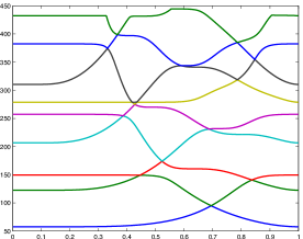
(a) $a$ moving on the symmetry axis of the angular sector

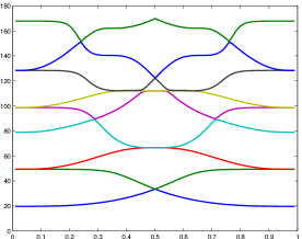
(b) $a$ moving on the diagonal of the square

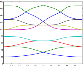
(c) $a$ moving on the mediane of the square

Figure 1. $a\mapsto\lambda_{k}^{(a,\frac{1}{2})}$, $k=1,\ldots,9$, in the angular sector and the square

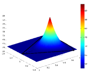
(a) $a\mapsto\lambda_{1}^{(a,\frac{1}{2})}$

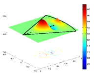
(b) $a\mapsto\lambda_{2}^{(a,\frac{1}{2})}$

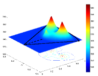
(c) $a\mapsto\lambda_{3}^{(a,\frac{1}{2})}$

Figure 2. Three-dimensional vision of $\lambda_{k}^{(a,\frac{1}{2})}$, $k=1,\ldots,3$, for the angular sector

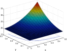
(a) $a\mapsto\lambda_{1}^{(a,\frac{1}{2})}$

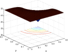
(b) $a\mapsto\lambda_{2}^{(a,\frac{1}{2})}$

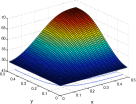
(c) $a\mapsto\lambda_{3}^{(a,\frac{1}{2})}$

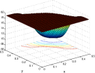
(d) $a\mapsto\lambda_{4}^{(a,\frac{1}{2})}$

Figure 3. Three-dimensional vision of $\lambda_{k}^{(a,\frac{1}{2})}$, $k=1,\ldots,4$, for the square

Since Theorem 1.6 is related to local properties of the associated eigenfunctions by means of conditions $(i)$–$(ii)$, we also present in Figure 4 the graphs of the nodal set of eigenfunctions in the square when the singular pole is at its center. In the case of the disk, we refer to [10, Figures 7 and 8].

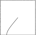
(a) $\varphi_{1}^{(0,\frac{1}{2})}$

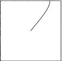
(b) $\varphi_{2}^{(0,\frac{1}{2})}$

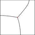
(c) $\varphi_{3}^{(0,\frac{1}{2})}$

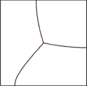
(d) $\varphi_{4}^{(0,\frac{1}{2})}$

Figure 4. Nodal set of the first four eigenfunctions in the square with singular pole at the center

We present here a collection of observations on these simulations.

• When the singular pole is at the center of the square, or the disk, see [10, Figures 7 and 8], the eigenvalues are always of multiplicity two.

• For the angular sector, the points where eigenvalues are not simple correspond to points where they are not differentiable. Indeed, we see in Figure 1(a) and Figure 2 that the meeting points present a structure of a singular cone. Moreover, when the same thing happens in the square, at those points there is only one nodal line for the corresponding eigenfunctions (see Figure 1(b) and (c) and Figure 4).

• For the square and the disk, if the singular pole is at the center, two cases occur. In the first case eigenvalues are not differentiable at that point and the corresponding eigenfunctions have exactly one nodal line. This is for example the case for the first and second eigenvalues, where we note the structure of non differentiable cone in Figures 1, 3 (a) and (b), and the unique nodal line in Figure 4 (a) and (b). In the second case eigenvalues are differentiable, and the corresponding eigenfunctions have more nodal lines. This happens for instance for the third and fourth eigenvalues, see Figures 1, 3 (c) and (d) and Figure 4 (c) and (d).

• The two linearly independent eigenfunctions corresponding to the same eigenvalue always have the same number of nodal lines ending at the singular point; moreover, those lines leave the point in opposite directions, therefore never in a tangential way. This can be seen in Figure 4 and in [10, Figure 8].

• When considering only variations of the position of the pole, it seems that the set

  $$\{a\in\Omega\,:\,\lambda_{k}^{(a,\nicefrac{{1}}{{2}})}\text{ is an eigenvalue of }(i\nabla+A_{a}^{\nicefrac{{1}}{{2}}})^{2}\text{ of multiplicity two}\}$$

  is a finite collection of points in $\Omega$.

• Points of multiplicity higher than two seem not to happen.

Observations (b), (c) and (d) suggest that there may be a relation between the number of nodal lines of the two eigenfunctions and the way the graphs of two subsequent eigenvalues meet at the multiple point. Indeed, when they both have one nodal line leaving the point in opposite directions, the lines in Figure 1 meet transversally and with a non vanishing derivative on the two branches, while if there is more than one nodal line, the lines in Figure 1 meet not transversally and with a vanishing derivative. This reminds us Theorem 1.3, where the criticality of the simple eigenvalues is related to the number of nodal lines of the corresponding eigenfunctions. For the derivatives at multiple eigenvalues when the domain is perturbed by means of a regular vector field, we refer the reader to the book of Henrot [16].

By observation (a), we foresee that all the eigenvalues are double because of the strong symmetries of the domain. As well, we think that the existence of multiple points such that the eigenvalue is differentiable (and then where the eigenfunctions have more than one nodal lines) can also be explained by those symmetries.

In view of observation (e), our main Theorem 1.6 provide a stronger analysis involving the combined parameters $(a,\alpha)$. However, it provides a local result around the point $(0,\tfrac{1}{2})$, and there chances to extend it in order to obtain a global result for every circulation $\alpha$. The analysis performed in our paper and the results achieved leave several other open questions. At the present time, we are not able to consider vanishing orders of the eigenfunctions greater than $1/2$ (i.e. the cases where the eigenfunctions have more than one nodal lines), but simulations suggest that multiple points are isolated even in these situations. By the way, simulations performed in [11, Section 7] and [9] suggest that high orders of vanishing for eigenfunctions may only occur when the domain $\Omega$ has strong symmetries (e.g. the disk or the square). On the other hand, as far as we know, two linearly independent orthogonal eigenfunctions corresponding to the same eigenvalue may have different orders of vanishing, but the available simulations do not show such a situation. The other fundamental assumption which plays a role in Theorem 1.6 is condition $(ii)$, which prevents the eigenfunctions nodal lines to be tangent. How general the assumptions of Theorem 1.6 can be is currently under investigation by the authors.

The paper is organized as follows. We devote Section 3 to illustrate the main differences between half-integer and non half-integer circulations. In Section 4 we prove the complex version of the abstract theorem from [20]. Section 5 gives us the perturbation of the domain used to obtain new operators with fixed definition domains. In Section 6, we prove Theorem 1.5 which gives first a continuity result for the eigenvalues with respect to the combined parameters $(a,\alpha)$, and next a regularity results for simple eigenvalues, with respect to the same parameters. Section 7 is (with Section 5) the most technical of the paper. We give therein the explicit form of the spectrally equivalent operators to $(i\nabla+A_{a}^{\alpha})^{2}$ (and its inverse). Finally, in Section 8, we make all the explicit computations using the local asymptotic behavior of the eigenfunctions (1.3) and use the abstract Theorem to prove our main result Theorem 1.6.

2. Preliminaries

2.1. Functional spaces

We notice that throughout the paper (except for Subsection 6.2), all the Hilbert spaces are complex Hilbert spaces, i.e. they have complex scalar products.

If $\Omega\subset\mathbb{R}^{2}$ is open, bounded and simply connected, for $a\in\Omega$, we define the functional space $H^{1,a}(\Omega,\mathbb{C})$ as the completion of $\{u\in H^{1}(\Omega,\mathbb{C})\cap C^{\infty}(\Omega,\mathbb{C})\,:\,u\text{ vanishes in a neighborhood of }a\}$ with respect to the norm

$$\|u\|_{H^{1,a}(\Omega,\mathbb{C})}:=\left(\|\nabla u\|_{L^{2}(\Omega,\mathbb{C}^{2})}^{2}+\|u\|_{L^{2}(\Omega,\mathbb{C})}^{2}+\left\|\frac{u}{|x-a|}\right\|_{L^{2}(\Omega,\mathbb{C})}^{2}\right)^{1/2}.$$

When the circulation $\alpha$ is not an integer, i.e. $\alpha\in\mathbb{R}\setminus\mathbb{Z}$, the latter norm is equivalent to the norm

$$\|u\|_{H^{1,a}(\Omega,\mathbb{C})}=\left(\left\|(i\nabla+A_{a}^{\alpha})u\right\|^{2}_{L^{2}(\Omega,\mathbb{C}^{2})}+\|u\|^{2}_{L^{2}(\Omega,\mathbb{C})}\right)^{\!\!1/2},$$

in view of the Hardy type inequality proved in [17] (see also [8] and [12, Lemma 3.1 and Remark 3.2])

$$\int_{D_{r}(a)}|(i\nabla+A_{a}^{\alpha})u|^{2}\,dx\geq\Big{(}\min_{j\in\mathbb{Z}}|j-\alpha|\Big{)}^{2}\int_{D_{r}(a)}\frac{|u(x)|^{2}}{|x-a|^{2}}\,dx,$$

which holds for all $r>0$, $a\in\mathbb{R}^{2}$ and $u\in H^{1,a}(D_{r}(a),\mathbb{C})$. Here we denote as $D_{r}(a)$ the disk of center $a$ and radius $r$.

As well, the space $H^{1,a}_{0}(\Omega,\mathbb{C})$ is defined as the completion of $C^{\infty}_{c}(\Omega\setminus\{a\},\mathbb{C})$ with respect to the norm $\|u\|_{H^{1,a}(\Omega,\mathbb{C})}$. By a Poincaré type inequality, see e.g. [4, A.3], we can consider the following equivalent norm on $H^{1,a}_{0}(\Omega,\mathbb{C})$

$$\|u\|_{H^{1,a}_{0}(\Omega,\mathbb{C})}:=\left(\|(i\nabla+A_{a}^{\alpha})u\|_{L^{2}(\Omega,\mathbb{C}^{2})}^{2}\right)^{1/2}.$$

Finally, $(H^{1,a}_{0}(\Omega,\mathbb{C}))^{\star}$ is the space dual to $H^{1,a}_{0}(\Omega,\mathbb{C})$. We emphasize that as long as $\alpha$ is not an integer, those spaces are independent of $\alpha$.

2.2. Eigenvalues and eigenfunctions

We look at the operator defined in (1.2)

$$(i\nabla+A_{a}^{\alpha})^{2}\,:\,H^{1,a}_{0}(\Omega,\mathbb{C})\to(H^{1,a}_{0}(\Omega,\mathbb{C}))^{\star}.$$

In a standard way, for any $u\in H^{1,a}_{0}(\Omega,\mathbb{C})$, $(i\nabla+A_{a}^{\alpha})^{2}u$ acts in the following way

$$\phantom{a}_{(H^{1,a}_{0}(\Omega,\mathbb{C}))^{\star}}\left\langle(i\nabla+A_{a}^{\alpha})^{2}u,v\right\rangle_{H^{1,a}_{0}(\Omega,\mathbb{C})}:=\int_{\Omega}(i\nabla+A_{a}^{\alpha})u\cdot\overline{(i\nabla+A_{a}^{\alpha})v}.$$ (2.1)

By standard spectral theory the inverse operator

$$[(i\nabla+A_{a}^{\alpha})^{2}]^{-1}\circ\text{Im}_{H^{1,a}_{0}(\Omega,\mathbb{C})\to(H^{1,a}_{0}(\Omega,\mathbb{C}))^{\star}}\,:\,H^{1,a}_{0}(\Omega,\mathbb{C})\to H^{1,a}_{0}(\Omega,\mathbb{C})$$

is compact because of the compactness of the embedding $\text{ Im}_{H^{1,a}_{0}(\Omega,\mathbb{C})\to(H^{1,a}_{0}(\Omega,\mathbb{C}))^{\star}}$ coming from the compact embedding

$$H^{1,a}_{0}(\Omega,\mathbb{C})\hookrightarrow L^{2}(\Omega,\mathbb{C}),$$

and the continuity of the immersion $L^{2}(\Omega,\mathbb{C})\hookrightarrow(H^{1,a}_{0}(\Omega,\mathbb{C}))^{\star}$, see e.g. [25].

We are considering the eigenvalue problem

$$\begin{cases}(i\nabla+A_{a}^{\alpha})^{2}u=\lambda u,&\text{in }\Omega,\\ u=0,&\text{on }\partial\Omega,\end{cases} E_{a,\alpha}$$ ()

in a weak sense, and we say that $\lambda\in\mathbb{C}$ is an eigenvalue of problem ($E_{a,\alpha}$) if there exists $u\in H^{1,a}_{0}(\Omega,\mathbb{C})\setminus\{0\}$ (called eigenfunction) such that

$$\int_{\Omega}(i\nabla+A_{a}^{\alpha})u\cdot\overline{(i\nabla+A_{a}^{\alpha})v}\,dx=\lambda\int_{\Omega}u\overline{v}\,dx\quad\text{ for all }v\in H^{1,a}_{0}(\Omega,\mathbb{C}).$$

From classical spectral theory (using the self-adjointness of the operator and the compactness of the inverse operator), for every $(a,\alpha)\in\Omega\times\mathbb{R}$, the eigenvalue problem ($E_{a,\alpha}$) admits a diverging sequence of real and positive eigenvalues $\{\lambda_{k}^{(a,\alpha)}\}_{k\geq 1}$ with finite multiplicity. In the enumeration

$$0<\lambda_{1}^{(a,\alpha)}\leq\lambda_{2}^{(a,\alpha)}\leq\dots\leq\lambda_{k}^{(a,\alpha)}\leq\dots$$

we repeat each eigenvalue as many times as its multiplicity. Those eigenvalues also have a variational characterization given by

$$\begin{split}\lambda_{k}^{(a,\alpha)}=\min\Big{\{}\sup_{u\in W_{k}\setminus\{0\}}\frac{\int_{\Omega}|(i\nabla+A_{a}^{\alpha})u|^{2}}{\int_{\Omega}|u|^{2}}\,:\,&W_{k}\text{ is a linear subspace of }H^{1,a}_{0}(\Omega,\mathbb{C}),\\ &\,\text{dim}W_{k}=k\Big{\}}.\end{split}$$ (2.2)

We denote by $\varphi_{k}^{(a,\alpha)}\in H^{1,a}_{0}(\Omega,\mathbb{C})$ the corresponding eigenfunctions orthonormalized in $L^{2}(\Omega,\mathbb{C})$. We note that if $\varphi_{k}^{(a,\alpha)}$ is an eigenfunction of $(i\nabla+A_{a}^{\alpha})^{2}$ of eigenvalue $\lambda_{k}^{(a,\alpha)}$, it is also an eigenfunction of $[(i\nabla+A_{a}^{\alpha})^{2}]^{-1}\circ\text{ Im}_{H^{1,a}_{0}(\Omega,\mathbb{C})\to(H^{1,a}_{0}(\Omega,\mathbb{C}))^{\star}}$ with eigenvalue $(\lambda_{k}^{(a,\alpha)})^{-1}$.

3. The gauge invariance

Among all the circulations $\alpha\in\mathbb{R}$, the case $\alpha\in\{1/2\}+\mathbb{Z}$ presents very special features. For the reader’s convenience, in this Section we are recalling some basic facts about eigenfunctions of Aharonov–Bohm operators. We gain them partially as they are stated in [3, Section 3].

3.1. General facts on the gauge invariance

Definition 3.1.

We call gauge function a smooth complex valued function $\psi\,:\,\Omega\to\mathbb{C}$ such that $|\psi|\equiv 1$. To any gauge function $\psi$, we associate a gauge transformation acting on the pairs magnetic potential – function as $(A,u)\mapsto(A^{*},u^{*})$, with

$$A^{*}=A+i\frac{\nabla\psi}{\psi},$$

$$u^{*}=\overline{\psi}u,$$

where $\nabla\psi=\nabla(\mathop{\mathfrak{Re}}\psi)+i\nabla(\mathop{\mathfrak{Im}}\psi)$. We notice that since $|\psi|=1$, $i\frac{\nabla\psi}{\psi}$ is a real vector field. Two magnetic potentials are said to be gauge equivalent if one can be obtained from the other by a gauge transformation (this is an equivalence relation).

The following result is a consequence, see [18, Theorem 1.2].

Proposition 3.2.

If $A$ and $A^{*}$ are two gauge equivalent vector potentials, the operators $(i\nabla+A)^{2}$ and $(i\nabla+A^{*})^{2}$ are unitarily equivalent, that is

$$\overline{\psi}\,(i\nabla+A)^{2}\,{\psi}=(i\nabla+A^{*})^{2}.$$

We immediately see that if $A$ and $A^{*}$ are gauge equivalent, then the corresponding operators are spectrally equivalent, i.e. they have the same spectrum, and in particular they have the same eigenvalues with the same multiplicity. The equivalence between two vector potentials (which is equivalent to the fact that their difference is gauge equivalent to $0$) can be determined using the following criterion.

Lemma 3.3.

Let $A$ be a vector potential in $\Omega$. It is gauge equivalent to $0$ if and only if

$$\frac{1}{2\pi}\oint_{\gamma}A(s)\cdot d\mathbf{s}\in\mathbb{Z}$$

for every closed path $\gamma$ contained in $\Omega$.

Whenever the vector potential $A$ is gauge equivalent to 0, i.e. there is a gauge function $\psi$ such that $A=-i\frac{\nabla\psi}{\psi}$, we can define the antilinear antiunitary operator $K$ by

$$Ku=\psi\bar{u}.$$ (3.1)

Definition 3.4.

We say that a function $u\in L^{2}(\Omega,\mathbb{C})$ is $K$-real when $Ku=u$.

3.2. Aharonov–Bohm potentials

When the circulation $\alpha=n$ is an integer, i.e.

$$\frac{1}{2\pi}\oint_{\gamma}A_{a}^{n}\cdot d\mathbf{s}\in\mathbb{Z},$$

for any closed path $\gamma$ contained in $\Omega$, it directly holds by Lemma 3.3 that $A_{a}^{n}$ is gauge equivalent to $0$. Moreover, in that particular case, we can give an explicit expression to the gauge function of Definition 3.1. For any $a\in\mathbb{R}^{2}$, we define $\theta_{a}\,:\,\mathbb{R}^{2}\setminus\{a\}\to[0,2\pi)$ the polar angle centred at $a$ such that

$$\theta_{a}(a+r(\cos t,\sin t))=t,\quad\text{ for }t\in[0,2\pi).$$ (3.2)

We remark that such an angle is regular except on the half-line

$$\{(x_{1},x_{2})\in\mathbb{R}^{2}\,:\,x_{2}=a_{2},\,x_{1}>a_{1}\}.$$

From relation (3.2) we immediately observe that for any $n\in\mathbb{Z}$

$$A_{a}^{n}=-ie^{-in\theta_{a}}\nabla e^{in\theta_{a}}=n\nabla\theta_{a},$$ (3.3)

almost everywhere. Therefore the gauge function is given by the phase $e^{in\theta_{a}}$ and such a phase is well defined and smooth thanks to the fact that the circulation $\alpha=n$ is an integer. Proposition 3.2 tells us then that, for any $n\in\mathbb{Z}$, $(i\nabla+A_{a}^{n})^{2}$ and $-\Delta$ are unitarily equivalent, i.e. the spectrum of $(i\nabla+A_{a}^{n})^{2}$ coincides with the spectrum of $-\Delta$.

Moreover the same gauge transformation tells us that, for any $\alpha\in(0,1)$ and $n\in\mathbb{Z}$, $(i\nabla+A_{a}^{\alpha})^{2}$ and $(i\nabla+A_{a}^{\alpha+n})^{2}$ are unitarily equivalent, i.e. the spectrum of $(i\nabla+A_{a}^{\alpha})^{2}$ coincides with the spectrum of $(i\nabla+A_{a}^{\alpha+n})^{2}$. Those observations tell us that it is sufficient to consider magnetic potentials with circulations $\alpha\in(0,1)$ since the other ones can be recovered from them, and $\alpha$ integer does not present any interest. This will be the case in the rest of the paper.

However, amoung the circulations $\alpha\in(0,1)$, the case $\alpha=1/2$ presents special features. We refer to [12, 15] for details. For any magnetic potential $A_{a}^{\nicefrac{{1}}{{2}}}$ defined in (1.1) it holds that

$$\frac{1}{2\pi}\oint_{\gamma}2A_{a}^{\nicefrac{{1}}{{2}}}\cdot d\mathbf{s}=\frac{1}{2\pi}\oint_{\gamma}A_{a}^{1}\cdot d\mathbf{s}=1\in\mathbb{Z},$$

for any closed path $\gamma$ containing $a$, so that, by Lemma 3.3, $2A_{a}^{\nicefrac{{1}}{{2}}}$ is gauge equivalent to $0$. Therefore, by Definition 3.1 and (3.2)–(3.3)

$$2A_{a}^{\nicefrac{{1}}{{2}}}=-ie^{-i\theta_{a}}\nabla e^{i\theta_{a}}=\nabla\theta_{a}.$$

We write the antilinear and antiunitary operator of (3.1), which depends on the position of the pole $a\in\Omega$ through the angle $\theta_{a}$, as

$$K_{a}u=e^{i\theta_{a}}\overline{u}.$$ (3.4)

For all $u\in C^{\infty}_{0}({\Omega\setminus\{a\}},\mathbb{C})$ we have

$$\begin{split}(i\nabla+A_{a}^{\nicefrac{{1}}{{2}}})(K_{a}u)&=(i\nabla+A_{a}^{\nicefrac{{1}}{{2}}})(e^{i\theta_{a}}\bar{u})=e^{i\theta_{a}}\left(i\nabla+i\frac{\nabla e^{i\theta_{a}}}{e^{i\theta_{a}}}+A_{a}^{\nicefrac{{1}}{{2}}}\right)\bar{u}\\ &=e^{i\theta_{a}}\left(i\nabla-A_{a}^{\nicefrac{{1}}{{2}}}\right)\bar{u}=-e^{i\theta_{a}}\overline{\left(i\nabla+A_{a}^{\nicefrac{{1}}{{2}}}\right)u}=-K_{a}((i\nabla+A_{a}^{\nicefrac{{1}}{{2}}})u),\end{split}$$ (3.5)

and therefore $(i\nabla+A_{a}^{\nicefrac{{1}}{{2}}})^{2}$ and $K_{a}$ commute

$$(i\nabla+A_{a}^{\nicefrac{{1}}{{2}}})^{2}\circ K_{a}=K_{a}\circ(i\nabla+A_{a}^{\nicefrac{{1}}{{2}}})^{2}.$$ (3.6)

Let us denote

$$L^{2}_{K_{a}}(\Omega,\mathbb{C}):=\{u\in L^{2}(\Omega,\mathbb{C})\,:\,K_{a}u=u\}.$$

The restriction of the scalar product to $L^{2}_{K_{a}}(\Omega,\mathbb{C})$ gives it the structure of a real Hilbert space, instead of a complex space. Relation (3.6) implies that $L^{2}_{K_{a}}(\Omega,\mathbb{C})$ is stable under the action of $(i\nabla+A_{a}^{\nicefrac{{1}}{{2}}})^{2}$; we denote by $(i\nabla+A_{a}^{\nicefrac{{1}}{{2}}})^{2}_{L^{2}_{K_{a}}(\Omega,\mathbb{C})}$ the restriction of $(i\nabla+A_{a}^{\nicefrac{{1}}{{2}}})^{2}$ to $L^{2}_{K_{a}}(\Omega,\mathbb{C})$, which is a real operator. There exists an orthonormal basis of $L^{2}_{K_{a}}(\Omega,\mathbb{C})$ formed by eigenfunctions of $(i\nabla+A_{a}^{\nicefrac{{1}}{{2}}})^{2}_{L^{2}_{K_{a}}(\Omega,\mathbb{C})}$.

We notice that if $u\in C^{\infty}_{0}(\Omega\setminus\{a\},\mathbb{C})$ is $K_{a}$-real, i.e. $K_{a}u=u$, relation (3.5) becomes

$$(i\nabla+A_{a}^{\nicefrac{{1}}{{2}}})u=-e^{i\theta_{a}}\overline{(i\nabla+A_{a}^{\nicefrac{{1}}{{2}}})u}.$$ (3.7)

Being allowed to consider $K_{a}$-real eigenfunctions of $(i\nabla+A_{a}^{\nicefrac{{1}}{{2}}})^{2}$ means to work with the real operator $(i\nabla+A_{a}^{\nicefrac{{1}}{{2}}})^{2}_{L^{2}_{K_{a}}(\Omega,\mathbb{C})}$ in the real space $L^{2}_{K_{a}}(\Omega,\mathbb{C})$. This leads to the special characterisation of the eigenfunctions for $\alpha=1/2$ mentioned in (1.3). Indeed, let $u$ be a $K_{a}$-real eigenfunction of $(i\nabla+A_{a}^{\nicefrac{{1}}{{2}}})^{2}$ of eigenvalue $\lambda$. If we consider the double covering manifold, already introduced in [15], (where we use the equivalence $\mathbb{R}^{2}\cong\mathbb{C}$) given by

$$\Omega_{a}:=\{y\in\mathbb{C}\,:\,y^{2}+a=x\in\Omega\},$$

and if we define for $y\in\Omega_{a}$ the function

$$v(y):=e^{-i\frac{\theta_{a}}{2}(y^{2}+a)}u(y^{2}+a)=e^{-i\theta_{0}(y)}u(y^{2}+a),$$ (3.8)

we have that $v$ is well defined in $\Omega_{a}$ since

$$e^{-i\frac{\theta_{a}}{2}(y^{2}+a)}=e^{-i\theta_{0}(y)}\text{ is well defined on }\Omega_{a}.$$

Morever, $v$ is real (this comes directly from the $K_{a}$-reality of $u$) and it is a weighted eigenfunction of $-\Delta$ in $\Omega_{a}$, i.e.

$$-\Delta v=4|y|^{2}\lambda v\quad\text{ in }\Omega_{a}.$$

To this aim see also [11, Lemma 2.3] and references therein.

Finally, from (3.8) it follows that $v$ is antisymmetric with respect to the transformation $y\mapsto-y$. From the above facts, we conclude that the nodal set of $u$, $u^{-1}(\{0\})$ (which coincides with the nodal set of $v$), is made of curves. Moreover, from the antisymmetry of $v$, we deduce that $u$ always has an odd number of nodal lines at $a$, and then at least one. As showed in [12, Theorem 6.3] if we denote by $h\in\mathbb{N}$, $h$ odd, the number of nodal lines of $u$ ending at $a\in\Omega$, there exist $c$, $d\in\mathbb{R}$ with $c^{2}+d^{2}\neq 0$, and

$$r^{-h/2}u(a+r(\cos t,\sin t))\to e^{i\frac{t}{2}}\left(c\cos\frac{ht}{2}+d\sin\frac{ht}{2}\right),$$

as $r\to 0^{+}$ in $C^{1,\tau}([0,2\pi],\mathbb{C})$ for any $\tau\in(0,1)$. Similarly, we can write

$$u(a+r(\cos t,\sin t))=r^{h/2}e^{i\frac{t}{2}}\left(c\cos\frac{ht}{2}+d\sin\frac{ht}{2}\right)+f(r,t),$$

as $r\to 0^{+}$, where $f(r,t)=O(r^{h/2+1})$ uniformly in $t\in[0,2\pi]$. The fact that $c$ and $d\in\mathbb{R}$ comes from the $K_{a}$-reality of $u$.

When $A_{a}^{\alpha}$ defined in (1.1) has circulation $\alpha\in(0,1)\setminus\{1/2\}$, we still have that

$$\frac{1}{\alpha}A_{a}^{\alpha}=-ie^{-i\theta_{a}}\nabla e^{i\theta_{a}},$$

for $\theta_{a}$ defined in (3.2). However, the main difference is that we loose the commutation property between $(i\nabla+A_{a}^{\alpha})^{2}$ and $K_{a}$ (given in (3.4)). This means that we cannot consider a basis of $K_{a}$-real eigenfunctions of $L_{K_{a}}^{2}(\Omega,\mathbb{C})$ and we must consider $(i\nabla+A_{a}^{\alpha})^{2}$ as a complex operator, and the special expression (1.3) with real coefficients does not hold.

4. Abstract result

In order to prove our results, we follow the strategy of [20]. The proof therein relies on a strong abstract result obtained by means of transversality theorems, see e.g. [13, p28]. We need a slightly different version of their abstract theorem, that we enounce and prove here.

Theorem 4.1.

Consider a Banach space $B$ and a complex Hilbert space $X$ with scalar product $(\cdot,\cdot)_{X}$. Let $V$ be a neighborhood of 0 in $B$ and consider a family of self-adjoint compact linear operators $\mathcal{T}_{b}\,:\,X\to X$ parametrized in $V$. Let $\lambda_{0}$ be an eigenvalue of $\mathcal{T}_{0}$ of multiplicity $\mu>1$ and denote by $\{x_{1}^{0},\ldots,x_{\mu}^{0}\}$ an orthonormal system of eigenvectors associated to $\lambda_{0}$. Suppose that the following two conditions hold

• the map $b\mapsto\mathcal{T}_{b}$ is $C^{1}$ in $V$;

• the application $F\,:\,B\to L_{h}(\mathbb{R}^{n},\mathbb{R}^{n})$ defined as $b\mapsto((\mathcal{T}^{\prime}(0)[b])x_{i}^{0},x_{j}^{0})_{X\,\{i,j=1,\ldots,\mu\}}$ is such that

  $$\mathrm{Im}F+[I]=L_{h}(\mathbb{R}^{\mu},\mathbb{R}^{\mu}).$$

Then

$$\{b\in B\,:\,\text{ there exists }\lambda_{b}\text{ eigenvalue of }\mathcal{T}_{b}\text{ near }\lambda_{0}\text{ of multiplicity }\mu\}$$

is a manifold in $B$ of codimension $\mu^{2}-1$.

Proof of Theorem 4.1.

For sake of clarity we sketch here the proof of the result, which follows the guidelines of its real counterpart contained in [20, Theorem 1].

Let us denote by $L_{h}(X,X)$ the set of all linear continuous hermitian operators from $X$ to $X$ and by $\Phi_{0}(X,X)$ the set of all Fredholm operators of index $0$. We define the set

$$F_{\mu,\mu}:=\{L\in\Phi_{0}\cap L_{h}(X,X)\,:\,\textrm{dim}\,\textrm{ker}L=\textrm{codim}\,\textrm{rk}L=\mu\}.$$

We remind that for any $L\in\Phi_{0}$ we have $X=\textrm{ker}L\oplus\textrm{rk}L$. We now fix $L_{0}\in F_{\mu,\mu}$ and define the orthogonal projections

$$P\,:\,X\to\textrm{ker}L_{0}\qquad Q\,:\,X\to\textrm{rk}L_{0}$$

and the spaces

$$V_{0}:=\{H\in L_{h}(X,X)\,:\,H(\textrm{ker}L_{0})\subset\textrm{rk}L_{0}\}\qquad M:=\{PHP\in L_{h}(X,X)\,:\,H\in L_{h}(X,X)\}.$$

Then [20, Lemma 1] applies providing $L_{h}(X,X)=V_{0}\oplus M$.

Remark 4.2.

We remark that $\mathrm{dim}M=\mu^{2}$ since $L_{h}(X,X)$ is a real vector space and not a complex vector space, and not $\mu(\mu+1)/2$ as in [20, Remark 1], where real Hilbert spaces $X$ were considered.

Then [20, Lemma 2] applies providing that $F_{\mu,\mu}$ is an analytic manifold of real codimension $\mu^{2}$ in $L_{h}(X,X)$; moreover, the tangent plane at $L_{0}$ to $F_{\mu,\mu}$ is $V_{0}$.

The next step consists in [20, Lemma 3]. Let $L_{0}\in F_{\mu,\mu}$ be such that $\mathrm{ker}L_{0}$ is not contained in $\mathrm{rk}L_{0}$. Then there exists a neighborhood $U$ of $L_{0}$ in $L_{h}(X,X)$ such that

$$\widetilde{F}_{\mu,\mu}:=\{L+\lambda I_{X}\,:\,L\in U\cap F_{\mu,\mu},\ \lambda\in\mathbb{R}\}$$

is a manifold, the tangent plane at $L_{0}$ to $\widetilde{F}_{\mu,\mu}$ is $V_{0}\oplus[I_{X}]$ and the codimension of $\widetilde{F}_{\mu,\mu}$ in $L_{h}(X,X)$ is $\mu^{2}-1$. The proof follows as in [20, Lemma 3].

Remark 4.3.

We stress that in the definition of $\widetilde{F}_{\mu,\mu}$ we need $\lambda$ to be real in such a way that $\widetilde{F}_{\mu,\mu}$ is a subspace in $L_{h}(X,X)$ (indeed, if $\lambda\in\mathbb{C}\setminus\mathbb{R}$ then $\lambda I_{X}$ is not hermitian). This produces $-1$ in the codimension of $\widetilde{F}_{\mu,\mu}$ in $L_{h}(X,X)$ since $V_{0}$ does not contain $I_{X}$.

The manifold $\widetilde{F}_{\mu,\mu}$ is the analytic manifold to which we can apply the transversality theorem, see e.g. [13]. The fundamental assumption $(ii)$ in Theorem 4.1 implies that the map $b\mapsto\mathcal{T}_{b}$ is transversal at $0\in B$ to $\widetilde{F}_{\mu,\mu}$, i.e.

$$\mathrm{rk}\mathcal{T}^{\prime}(0)+\left([I_{X}]\oplus V_{0}\right)=L_{h}(X,X).$$

The end of the proof of Theorem 4.1 follows as in [20, Theorem 1]. ∎

5. The modified operator

5.1. The local perturbation

Let us fix $\overline{R}>0$ sufficiently small and such that $D_{2\overline{R}}(0)\subset\Omega$. Let $\xi\in C^{\infty}_{c}(\mathbb{R}^{2})$ be a cut-off function such that

$$0\leq\xi\leq 1,\quad\xi\equiv 1\text{ on }D_{\overline{R}}(0),\quad\xi\equiv 0\text{ on }\mathbb{R}^{2}\setminus D_{2\overline{R}}(0),\quad|\nabla\xi|\leq\frac{4}{\overline{R}}\text{ on }\mathbb{R}^{2}.$$ (5.1)

We define for $a\in D_{\overline{R}}(0)$ the local transformation $\Phi_{a}\in C^{\infty}(\mathbb{R}^{2},\mathbb{R}^{2})$ by

$$\Phi_{a}(x)=x+a\xi(x).$$ (5.2)

Notice that $\Phi_{a}(0)=a$ and that $\Phi_{a}^{\prime}$ is a perturbation of the identity

$$\Phi_{a}^{\prime}=I+a\otimes\nabla\xi=\begin{pmatrix}1+a_{1}\frac{\partial\xi}{\partial x_{1}}&a_{1}\frac{\partial\xi}{\partial x_{2}}\\ a_{2}\frac{\partial\xi}{\partial x_{1}}&1+a_{2}\frac{\partial\xi}{\partial x_{2}}\end{pmatrix},$$

so that

$$J_{a}(x):=\det(\Phi_{a}^{\prime})=1+a_{1}\frac{\partial\xi}{\partial x_{1}}+a_{2}\frac{\partial\xi}{\partial x_{2}}=1+a\cdot\nabla\xi.$$ (5.3)

Let $R=\overline{R}/32$. Then, if $a\in D_{R}(0)$, $\Phi_{a}$ is invertible, its inverse $\Phi_{a}^{-1}$ is also $C^{\infty}(\mathbb{R}^{2},\mathbb{R}^{2})$, see e.g. [23, Lemma 1], and it can be written as

$$\Phi_{a}^{-1}(y)=y-\eta_{a}(y).$$ (5.4)

Moreover, from (5.2) and (5.4) we have

$$\eta_{a}(y)=a\,\xi(y-\eta_{a}(y))\quad\text{ or equivalently }\quad\eta_{a}(\Phi_{a}(x))=a\,\xi(x).$$

From this relation we deduce that

$$\frac{\partial\eta_{a,i}}{\partial y_{j}}(\Phi_{a}(x))=\frac{1}{J_{a}(x)}a_{i}\frac{\partial\xi}{\partial x_{j}}(x).$$ (5.5)

Lemma 5.1.

Let $J_{a}$ be defined as in (5.3). The maps $(a,\alpha)\mapsto J_{a}$, $(a,\alpha)\mapsto\sqrt{J_{a}}$ and $(a,\alpha)\mapsto 1/\sqrt{J_{a}}$ are of class $C^{\infty}(D_{R}(0)\times(0,1),C^{\infty}(\mathbb{R}^{2}))$.

Proof.

We first notice that $J_{a}$ does not depend on the variable $\alpha$. Therefore we only need to study the regularity with respect to $a$. By (5.3), we read that $J_{a}$ is a polynomial in the variable $a$, whose coefficients are $C^{\infty}(\mathbb{R}^{2})$. Thus $J_{a}$ is an analytic function with respect to $a$ into the space $C^{\infty}(\mathbb{R}^{2})$. Moreover, as $a\in D_{R}(0)$, there exists a positive constant $C$ such that $J_{a}(x)\geq C>0$ uniformly with respect to $x\in\mathbb{R}^{2}$. This implies that even $a\mapsto\sqrt{J_{a}}$ and $a\mapsto 1/\sqrt{J_{a}}$ are of class $C^{\infty}(D_{R}(0),C^{\infty}(\mathbb{R}^{2}))$. From this we conclude. ∎

5.2. The perturbed operator

Lemma 5.2.

Let $(a,\alpha)\in D_{R}(0)\times(0,1)$. If $u\in H^{1,a}_{0}(\Omega,\mathbb{C})$, then $v=u\circ\Phi_{a}\in H^{1,0}_{0}(\Omega,\mathbb{C})$, and the following relation holds

$$[(i\nabla+A_{a}^{\alpha})^{2}u]\circ\Phi_{a}=[(i\nabla+A_{0}^{\alpha})^{2}+\mathcal{L}_{(a,\alpha)}](u\circ\Phi_{a}),$$ (5.6)

where the operator $[(i\nabla+A_{a}^{\alpha})^{2}u]\circ\Phi_{a}\,:\,H^{1,0}_{0}(\Omega,\mathbb{C})\to(H^{1,0}_{0}(\Omega,\mathbb{C}))^{\star}$ is defined by acting as

$$\begin{split}&\phantom{a}{}_{(H^{1,0}_{0}(\Omega,\mathbb{C}))^{\star}}\left\langle[(i\nabla+A_{a}^{\alpha})^{2}u]\circ\Phi_{a},w\right\rangle_{H^{1,0}_{0}(\Omega,\mathbb{C})}\\ &\qquad\qquad\qquad\qquad\qquad=\phantom{a}_{(H^{1,a}_{0}(\Omega,\mathbb{C}))^{\star}}\left\langle(i\nabla+A_{a}^{\alpha})^{2}u,(wJ_{a}^{-1})\circ\Phi_{a}^{-1}\right\rangle_{H^{1,a}_{0}(\Omega,\mathbb{C})}\end{split}$$ (5.7)

and where the linear operator $\mathcal{L}_{(a,\alpha)}\,:\,H^{1,0}_{0}(\Omega,\mathbb{C})\to(H^{1,0}_{0}(\Omega,\mathbb{C}))^{\star}$ acts as

$$\phantom{a}{}_{(H^{1,0}_{0}(\Omega,\mathbb{C}))^{\star}}\left\langle[(i\nabla+A_{0}^{\alpha})^{2}+\mathcal{L}_{(a,\alpha)}]v,w\right\rangle_{H^{1,0}_{0}(\Omega,\mathbb{C})}$$

$$=\int_{\Omega}\left[(i\nabla+A_{0}^{\alpha})v+F(a,\alpha)v\right]\cdot\overline{\left[(i\nabla+A_{0}^{\alpha})w+F(a,\alpha)w-iJ_{a}^{-1}w\nabla J_{a}+iJ_{a}^{-2}w(a\cdot\nabla J_{a})\nabla\xi\right]},$$

where

$$F(a,\alpha)v:=(A_{a}^{\alpha}\circ\Phi_{a}-A_{0}^{\alpha})v-iJ_{a}^{-1}(a\cdot\nabla v)\nabla\xi.$$ (5.8)

Finally the map $(a,\alpha)\in D_{R}(0)\times(0,1)\mapsto(i\nabla+A_{0}^{\alpha})^{2}+\mathcal{L}_{(a,\alpha)}\in BL(H^{1,0}_{0}(\Omega,\mathbb{C}),(H^{1,0}_{0}(\Omega,\mathbb{C}))^{\star}$ is of class $C^{\infty}$.

Proof.

The fact that $u\circ\Phi_{a}\in H^{1,0}_{0}(\Omega,\mathbb{C})$ if $u\in H^{1,a}_{0}(\Omega,\mathbb{C})$ follows easily using the definition of the functional space in Subsection 2.1 and (5.1), (5.3).

Using the definitions of $\mathcal{L}_{(a,\alpha)}$ in (5.6), (5.7) and the way $(i\nabla+A_{a}^{\alpha})^{2}$ acts in (2.1), it holds that

$$\phantom{a}_{(H^{1,0}_{0}(\Omega,\mathbb{C}))^{\star}}\left\langle[(i\nabla+A_{0}^{\alpha})^{2}+\mathcal{L}_{(a,\alpha)}]v,w\right\rangle_{H^{1,0}_{0}(\Omega,\mathbb{C})}=\int_{\Omega}(i\nabla+A_{a}^{\alpha})u\cdot\overline{(i\nabla+A_{a}^{\alpha})f},$$ (5.9)

where we set $u=v\circ\Phi_{a}^{-1}$ and $f=(wJ_{a}^{-1})\circ\Phi_{a}^{-1}$. Performing a change of variables in the right hand side of (5.9) and using the relation

$$[(i\nabla+A_{a}^{\alpha})u]\circ\Phi_{a}=i\nabla v-iJ_{a}^{-1}(a\cdot\nabla v)\nabla\xi+A_{0}^{\alpha}v+(A_{a}^{\alpha}\circ\Phi-A_{0}^{\alpha})v=(i\nabla+A_{0}^{\alpha})v+F(a,\alpha)v,$$

which holds true because of (5.5), we obtain that

$$\eqref{eq:formal}=\int_{\Omega}\left[(i\nabla+A_{0}^{\alpha})v+F(a,\alpha)v\right]\cdot\overline{\left[(i\nabla+A_{0}^{\alpha})z+F(a,\alpha)z\right]}\,J_{a},$$

where $z=f\circ\Phi_{a}=wJ_{a}^{-1}$. Finally, the claim follows using

$$J_{a}(i\nabla+A_{0}^{\alpha})z=(i\nabla+A_{0}^{\alpha})w-iJ_{a}^{-1}w\nabla J_{a}$$

and

$$J_{a}F(a,\alpha)z=F(a,\alpha)w+iJ_{a}^{-2}w(a\cdot\nabla J_{a})\nabla\xi.$$

Since $\xi(x)\equiv 1$ for every $x\in D_{R}(0)$, then for every $a\in D_{R}(0)$ and every $\alpha\in(0,1)$ $A_{a}^{\alpha}\circ\Phi_{a}-A_{0}^{\alpha}=0$ and $J_{a}\equiv 1$ for every $x\in D_{R}(0)$. Therefore we have that

$$\eqref{eq:formal} =\int_{D_{R}(0)}(i\nabla+A_{0}^{\alpha})v\cdot\overline{(i\nabla+A_{0}^{\alpha})z}$$

$$\quad+\int_{\Omega\setminus D_{R}(0)}\left[(i\nabla+A_{0}^{\alpha})v+F(a,\alpha)v\right]\cdot\overline{\left[(i\nabla+A_{0}^{\alpha})z+F(a,\alpha)z\right]}\,J_{a};$$

we then see that $A_{a}^{\alpha}\circ\Phi_{a}-A_{0}^{\alpha}$ is a $C^{1}(\Omega)$ function which depends $C^{\infty}$-regularly from the parameter $(a,\alpha)\in D_{R}(0)\times(0,1)$ (see also the argument in Lemma 5.1). In this way, the $\mathcal{L}_{(a,\alpha)}$ contribution is out of the disk $D_{R}(0)$ where singularities may occur and the fact that the map $(a,\alpha)\mapsto\mathcal{L}_{(a,\alpha)}$ is $C^{\infty}$ follows from this, (5.8) and Lemma 5.1. ∎

First we notice that

$$\mathcal{L}_{(0,\nicefrac{{1}}{{2}})}=0,$$

since $J_{0}=1$ and $F(0,\tfrac{1}{2})=0$. In fact, it also holds that $\mathcal{L}_{(0,\alpha)}=0$ for the same reasons. Since the map $(a,\alpha)\mapsto\mathcal{L}_{(a,\alpha)}$ is smooth, in the following we write for every $(b,t)\in\mathbb{R}^{2}\times\mathbb{R}$

$$\mathcal{L}^{\prime}(0,\tfrac{1}{2})[(b,t)]\,:\,H^{1,0}_{0}(\Omega,\mathbb{C})\to(H^{1,0}_{0}(\Omega,\mathbb{C}))^{\star},$$ (5.10)

the derivative of $\mathcal{L}_{(a,\alpha)}$ at the point $(0,\tfrac{1}{2})$, applied to $(b,t)$. Letting $\varepsilon:=\alpha-\tfrac{1}{2}$ it holds that

$$\mathcal{L}_{(a,\alpha)}=\mathcal{L}^{\prime}(0,\tfrac{1}{2})[(a,\varepsilon)]+o(|(a,\varepsilon)|),$$

as $|(a,\varepsilon)|\to 0$, so that $\mathcal{L}_{(a,\alpha)}=O(|(a,\varepsilon)|)$ in $BL(H^{1,0}_{0}(\Omega,\mathbb{C}),(H^{1,0}_{0}(\Omega,\mathbb{C}))^{\star})$ as $|(a,\varepsilon)|\to 0$.

6. Continuity of eigenvalues with respect to $(a,\alpha)$

6.1. Proof of Theorem 1.5: continuity

The proof is based on the variational characterization of the magnetic eigenvalues given by (2.2). We follow the same outline as in [11, Theorem 3.4].

Claim 1.

We aim at proving that if $(a_{0},\alpha_{0})\in\Omega\times(0,1)$ then

$$\limsup_{(a,\alpha)\to(a_{0},\alpha_{0})}\lambda_{k}^{(a,\alpha)}\leq\lambda_{k}^{(a_{0},\alpha_{0})}.$$

Proof of the claim.

It will be sufficient to find a $k$-dimensional linear subspace $E_{k}\subset H^{1,a}_{0}(\Omega,\mathbb{C})$ such that

$$\int_{\Omega}|(i\nabla+A_{a}^{\alpha})\Phi|^{2}\leq(\lambda_{k}^{(a_{0},\alpha_{0})}+\varepsilon(a,\alpha))\|\Phi\|_{L^{2}(\Omega)}^{2}\quad\text{ for every }\Phi\in E_{k},$$

where $\varepsilon(a,\alpha)\to 0$ as $(a,\alpha)\to(a_{0},\alpha_{0})$.

Let $\{\varphi_{1},\ldots,\varphi_{k}\}$ be a set of eigenfunctions respectively related to $\lambda_{1}^{(a_{0},\alpha_{0})},\ldots,\lambda_{k}^{(a_{0},\alpha_{0})}$. Given $r\in(0,1)$, $r:=2|a-a_{0}|$, let $\eta$ be a smooth cut-off function given by

$$\eta(x):=\begin{cases}0&\text{ for }0\leq|x|\leq r\\ \frac{\log r-\log|x|}{\log\sqrt{r}}&\text{ for }r\leq|x|\leq\sqrt{r}\\ 1&\text{ for }|x|\geq\sqrt{r}\end{cases}.$$

We denote $\eta_{a}(x):=\eta(x-a)$. By [11, Lemma 3.1] we have that

$$\int_{\mathbb{R}^{2}}(|\nabla\eta_{a}|^{2}+(1-{\eta_{a}}^{2}))\to 0\quad\text{ as }a\to a_{0}.$$

We define

$$E_{k}:=\text{span}\{\tilde{\varphi}_{1},\ldots,\tilde{\varphi}_{k}\}\quad\text{ where }\tilde{\varphi}_{j}:=e^{i\alpha(\theta_{a}-\theta_{a_{0}})}\eta_{a}\varphi_{j}.$$

By [11, Lemma 3.3], it holds that $\tilde{\varphi}_{j}\in H^{1,a}_{0}(\Omega,\mathbb{C})$. We consider an arbitrary combination $\Phi:=\sum_{j=1}^{k}\beta_{j}\tilde{\varphi}_{j}$ for $\beta_{j}\in\mathbb{C}$. We compute

$$\int_{\Omega}|(i\nabla+A_{a}^{\alpha})\Phi|^{2} =\int_{\Omega}\Big{|}\sum_{j=1}^{k}\beta_{j}(i\nabla+A_{a}^{\alpha})\tilde{\varphi}_{j}\Big{|}^{2}=\sum_{j,l=1}^{k}\beta_{j}\overline{\beta_{l}}\int_{\Omega}(i\nabla+A_{a_{0}}^{\alpha})^{2}(\eta_{a}\varphi_{j})\,(\eta_{a}\overline{\varphi_{l}})$$

$$=\sum_{j,l=1}^{k}\beta_{j}\overline{\beta_{l}}\int_{\Omega}\Big{(}\eta_{a}(i\nabla+A_{a_{0}}^{\alpha})^{2}\varphi_{j}+2i\nabla\eta_{a}\cdot(i\nabla+A_{a_{0}}^{\alpha})\varphi_{j}-\varphi_{j}\Delta\eta_{a}\Big{)}\,(\eta_{a}\overline{\varphi_{l}}).$$

Letting $\delta:=\alpha-\alpha_{0}$, we can rewrite it as

$$\int_{\Omega}|(i\nabla+A_{a}^{\alpha})\Phi|^{2} =\sum_{j,l=1}^{k}\beta_{j}\overline{\beta_{l}}\int_{\Omega}\Big{(}\eta_{a}(i\nabla+A_{a_{0}}^{\alpha_{0}})^{2}\varphi_{j}+2i\nabla\eta_{a}\cdot(i\nabla+A_{a_{0}}^{\alpha_{0}})\varphi_{j}-\varphi_{j}\Delta\eta_{a}\Big{)}(\eta_{a}\overline{\varphi_{l}})$$ (6.1)

$$+\delta\sum_{j,l=1}^{k}\beta_{j}\overline{\beta_{l}}\int_{\Omega}\Big{(}2i\eta_{a}A_{a_{0}}^{1}\cdot\nabla\varphi_{j}+(2\alpha_{0}+\delta)\eta_{a}|A_{a_{0}}^{1}|^{2}\varphi_{j}+2i\nabla\eta_{a}\cdot A_{a_{0}}^{1}\varphi_{j}\Big{)}(\eta_{a}\overline{\varphi_{l}}).$$ (6.2)

From [11, Theorem 3.4, Step 1] it follows that the first term

$$\eqref{eq:cont1}\leq(\lambda_{k}^{(a_{0},\alpha_{0})}+\varepsilon^{\prime}(a))\|\Phi\|^{2}_{L^{2}(\Omega)},$$ (6.3)

where $\varepsilon^{\prime}(a)\to 0$ as $a\to a_{0}$. For what concerns the second term (6.2), it will be sufficient to show that the integral appearing in (6.2) is uniformly bounded with respect to $a$. To this aim, we estimate

$$\left|\int_{\Omega}{\eta_{a}}^{2}A_{a_{0}}^{1}\overline{\varphi_{l}}\cdot\nabla\varphi_{j}\right|\leq C\left\|\frac{\varphi_{l}}{|x-a_{0}|}\right\|_{L^{2}(\Omega)}\,\||x-a_{0}|A_{a_{0}}^{1}\|_{L^{\infty}(\Omega)}\,\|\nabla\varphi_{j}\|_{L^{2}(\Omega)},$$

$$\left|\int_{\Omega}{\eta_{a}}^{2}\varphi_{j}\overline{\varphi_{l}}|A^{1}_{a_{0}}|^{2}\right|\leq C\left\|\frac{\varphi_{j}}{|x-a_{0}|}\right\|_{L^{2}(\Omega)}\,\left\|\frac{\varphi_{l}}{|x-a_{0}|}\right\|_{L^{2}(\Omega)},$$

$$\left|\int_{\Omega}{\eta_{a}}A_{a_{0}}^{1}\cdot\nabla\eta_{a}\varphi_{j}\overline{\varphi_{l}}\right|\leq\left\|\frac{\varphi_{j}}{|x-a_{0}|}\right\|_{L^{2}(\Omega)}\,\||x-a_{0}|A^{1}_{a_{0}}\|_{L^{\infty}(\Omega)}\,\|\nabla\eta_{a}\|_{L^{2}(\Omega)}\,\|\varphi_{l}\|_{L^{2}(\Omega)}.$$

Those three terms are uniformly bounded with respect to $a$. Therefore from [11, Lemma 3.3]

$$\eqref{eq:cont2}\leq\delta C\|\Phi\|^{2}_{L^{2}(\Omega)}\to 0\quad\text{ as }\delta=\alpha-\alpha_{0}\to 0,$$ (6.4)

for a constant $C>0$ independent of $(a,\delta)$.

The proof of the first step is concluded by (6.3)–(6.4). ∎

Claim 2.

We aim at proving that if $(a_{0},\alpha_{0})\in\Omega\times(0,1)$ then

$$\liminf_{(a,\alpha)\to(a_{0},\alpha_{0})}\lambda_{k}^{(a,\alpha)}\geq\lambda_{k}^{(a_{0},\alpha_{0})}.$$

Proof of the claim.

Consider $\{\varphi_{1}^{(a,\alpha)},\ldots,\varphi_{k}^{(a,\alpha)}\}$ be a set of orthonormalized eigenfunctions in $L^{2}(\Omega,\mathbb{C})$ and respectively related to $\lambda_{1}^{(a,\alpha)},\ldots,\lambda_{k}^{(a,\alpha)}$.

We first observe that Claim 1 implies for $j=1,\ldots,k$,

$$\|\varphi_{j}^{(a,\alpha)}\|_{H^{1}_{0}(\Omega,\mathbb{C})}\leq C\int_{\Omega}|(i\nabla+A_{a}^{\alpha})\varphi_{j}|^{2}\leq C\lambda_{j}^{(a_{0},\alpha_{0})},$$

for $(a,\alpha)$ sufficiently close to $(a_{0},\alpha_{0})$. Therefore there exist a sequence $(a_{n},\alpha_{n})\to(a_{0},\alpha_{0})$, as $n\to+\infty$, and functions $\varphi_{j}^{*}\in H^{1}_{0}(\Omega,\mathbb{C})$ such that

$$\begin{aligned} \varphi_{j}^{(a_{n},\alpha_{n})}\rightharpoonup\varphi_{j}^{*}\quad&\text{ in }H^{1}_{0}(\Omega,\mathbb{C})\\ \varphi_{j}^{(a_{n},\alpha_{n})}\to\varphi_{j}^{*}\quad&\text{ in }L^{2}(\Omega,\mathbb{C})\end{aligned}\quad\text{ as }n\to+\infty,$$

and $\int_{\Omega}\varphi_{j}^{*}\overline{\varphi}_{l}^{*}=0$ for $j\neq l$. Moreover, by Fatou’s Lemma and Claim 1 we have for any $j=1,\ldots,k$,

$$\left\|\frac{\varphi_{j}^{*}}{|x-a_{0}|}\right\|^{2}_{L^{2}(\Omega,\mathbb{C})} \leq\liminf_{n\to+\infty}\left\|\frac{\varphi_{j}^{(a_{n},\alpha_{n})}}{|x-a_{n}|}\right\|^{2}_{L^{2}(\Omega,\mathbb{C})}\leq C\liminf_{n\to+\infty}\int_{\Omega}|(i\nabla+A_{a_{n}}^{\alpha_{n}})\varphi_{j}^{(a_{n},\alpha_{n})}|^{2}\leq C\lambda_{j}^{(a_{0},\alpha_{0})},$$

so that $\varphi_{j}^{*}\in H^{1,a_{0}}_{0}(\Omega,\mathbb{C})$.

Up to a diagonal process, with a little abuse of notation, let us assume that for any $j=1,\ldots,k$

$$\lim_{n\to+\infty}\lambda_{j}^{(a_{n},\alpha_{n})}=\lambda_{j}^{*}=\liminf_{(a,\alpha)\to(a_{0},\alpha_{0})}\lambda_{j}^{(a,\alpha)}.$$

Thus, given a test function $\phi\in C^{\infty}_{0}(\Omega\setminus\{a_{0}\})$, if $n$ is large enough to have $a_{n}\not\in\text{supp}\phi$, we can pass to the limit along the above subsequence in the following expression

$$\int_{\Omega}\varphi_{j}^{(a_{n},\alpha_{n})}\,\overline{(i\nabla+A_{a_{n}}^{\alpha_{n}})^{2}\phi}=\lambda_{j}^{(a_{n},\alpha_{n})}\int_{\Omega}\varphi_{j}^{(a_{n},\alpha_{n})}\overline{\phi}$$

to obtain

$$\int_{\Omega}(i\nabla+A_{a_{0}}^{\alpha_{0}})^{2}\varphi_{j}^{*}\overline{\phi}=\lambda_{j}^{*}\int_{\Omega}\varphi_{j}^{*}\overline{\phi}.$$

By density, this is also valid for every $\phi\in H^{1,a_{0}}_{0}(\Omega,\mathbb{C})$, and therefore the orthogonality between the $\varphi_{j}^{*}$ follows.

Thus, we obtain that

$$\lambda_{k}^{(a_{0},\alpha_{0})} \leq\sup_{(c_{1},\ldots,c_{k})\in\mathbb{C}\setminus\{0\}}\frac{\int_{\Omega}\left|(i\nabla+A_{a_{0}}^{\alpha_{0}})\Big{(}\sum_{j=1}^{k}c_{j}\varphi_{j}^{*}\Big{)}\right|^{2}}{\int_{\Omega}\left|\sum_{j=1}^{k}c_{j}\varphi_{j}^{*}\right|^{2}}=\sup_{(c_{1},\ldots,c_{k})\in\mathbb{C}\setminus\{0\}}\frac{\sum_{j=1}^{k}|c_{j}|^{2}\lambda_{j}^{*}}{\sum_{j}|c_{j}|^{2}}\leq\lambda_{k}^{*},$$

and Claim 2 follows. ∎

The proof is thereby completed combining Claim 1 and 2.

Remark 6.1.

Following the scheme of [11, Section 4] it is also possible to prove that for any $k\in\mathbb{N}$ the map $(a,\alpha)\mapsto\lambda_{k}^{(a,\alpha)}$ is continuous up to the boundary of $\Omega\times(0,1)$.

6.2. Proof of Theorem 1.5: higher regularity for simple eigenvalues

Fix $\alpha_{0}\in(0,1)$ such that $\lambda_{k}^{(0,\alpha_{0})}$ is a simple eigenvalue. Throughout this subsection, we will treat for simplicity the space $H^{1,0}_{0}(\Omega,\mathbb{C})$ as a real Hilbert space endowed with the scalar product

$$(u,v):=\mathop{\mathfrak{Re}}\bigg{(}\int_{\Omega}(i\nabla+A_{0}^{\alpha_{0}})u\cdot\overline{(i\nabla+A_{0}^{\alpha_{0}})v}\bigg{)}.$$

To emphasize the fact that $H^{1,0}_{0}(\Omega,\mathbb{C})$ is meant as a vector space over $\mathbb{R}$, we denote it as $H^{1,0}_{0,\mathbb{R}}(\Omega,\mathbb{C})$. The main difference lies in the fact that if $u\in H^{1,0}_{0,\mathbb{R}}(\Omega,\mathbb{C})$, then $u$ and $iu$ are linearly independent, which was not the case in the complex vector space. We also write $(H^{1,0}_{0,\mathbb{R}}(\Omega,\mathbb{C}))^{\star}$ the real dual space of $H^{1,0}_{0,\mathbb{R}}(\Omega,\mathbb{C})$.

Let us consider the function $F\,:\,\Omega\times(0,1)\times H^{1,0}_{0,\mathbb{R}}(\Omega,\mathbb{C})\times\mathbb{C}\to(H^{1,0}_{0,\mathbb{R}}(\Omega,\mathbb{C}))^{\star}\times\mathbb{R}\times\mathbb{R}$ sending $(a,\alpha,\varphi,\lambda)$ on

$$\left((i\nabla+A_{0}^{\alpha})^{2}\varphi+\mathcal{L}_{(a,\alpha)}\varphi-\lambda\varphi,\,\mathop{\mathfrak{Re}}\int_{\Omega}\varphi\,\big{(}\overline{\varphi_{k}^{(0,\alpha)}\circ\Phi_{a}}\big{)}\,J_{a}-1,\,\mathfrak{Im}\int_{\Omega}\varphi\,\big{(}\overline{\varphi_{k}^{(0,\alpha)}\circ\Phi_{a}}\big{)}\,J_{a}\right),$$ (6.5)

where $(i\nabla+A_{0}^{\alpha})^{2}\varphi-\lambda\varphi\in(H^{1,0}_{0,\mathbb{R}}(\Omega,\mathbb{C}))^{\star}$ acts as

$$\phantom{a}{}_{(H^{1,0}_{0,\mathbb{R}}(\Omega,\mathbb{C}))^{\star}}\Big{\langle}(i\nabla+A_{0}^{\alpha})^{2}\varphi-\lambda\varphi,u\Big{\rangle}_{\!H^{1,0}_{0,\mathbb{R}}(\Omega,\mathbb{C})}\!\!=\mathop{\mathfrak{Re}}\left({\textstyle{\int_{\Omega}(i\nabla+A_{0}^{\alpha})\varphi\cdot\overline{(i\nabla+A_{0}^{\alpha})u}-\lambda\int_{\Omega}\varphi\overline{u}}}\right)$$

for all $\varphi\in H^{1,0}_{0,\mathbb{R}}(\Omega,\mathbb{C})$. We notice that in (6.5) $\mathbb{C}$ is also meant as a vector space over $\mathbb{R}$.

We have that for any $\alpha_{0}\in(0,1)$

$$F(0,\alpha_{0},\varphi_{k}^{(0,\alpha_{0})},\lambda_{k}^{(0,\alpha_{0})})=(0,0,0),$$

since $\Phi_{0}$ is the identity, $J_{0}=1$ and $\mathcal{L}_{(0,\alpha_{0})}=0$. Moreover, by direct calculations it is easy to verify that $F$ is $C^{\infty}$ with respect to $(\varphi,\lambda)$, at $(0,\alpha_{0},\varphi_{k}^{(0,\alpha_{0})},\lambda_{k}^{(0,\alpha_{0})})$ and moreover the explicit derivative of $F$ at $(0,\alpha_{0},\varphi_{k}^{(0,\alpha_{0})},\lambda_{k}^{(0,\alpha_{0})})$, applied to $(\varphi,\lambda)$, is given by

$$dF_{(\varphi,\lambda)}(0,\alpha_{0},\varphi_{k}^{(0,\alpha_{0})},\lambda_{k}^{(0,\alpha_{0})})[(\varphi,\lambda)]$$

$$\qquad=\left((i\nabla+A_{0}^{\alpha_{0}})^{2}\varphi-\lambda_{k}^{(0,\alpha_{0})}\varphi-\lambda\varphi_{k}^{(0,\alpha_{0})},\,\mathop{\mathfrak{Re}}\int_{\Omega}\varphi\,\overline{\varphi_{k}^{(0,\alpha_{0})}},\,\mathfrak{Im}\int_{\Omega}\varphi\,\overline{\varphi_{k}^{(0,\alpha_{0})}}\right)$$

for every $(\varphi,\lambda)\in H^{1,0}_{0,\mathbb{R}}(\Omega,\mathbb{C})\times\mathbb{C}$.

It remains to prove that $dF_{(\varphi,\lambda)}(0,\alpha_{0},\varphi_{k}^{(0,\alpha_{0})},\lambda_{k}^{(0,\alpha_{0})})\,:\,H^{1,0}_{0,\mathbb{R}}(\Omega,\mathbb{C})\times\mathbb{C}\to(H^{1,0}_{0,\mathbb{R}}(\Omega),\mathbb{C})^{\star}\times\mathbb{R}\times\mathbb{R}$ is invertible. For any $\lambda\in\mathbb{C}$, we define

$$T_{\lambda}\,:\,H^{1,0}_{0,\mathbb{R}}(\Omega,\mathbb{C})\to(H^{1,0}_{0,\mathbb{R}}(\Omega,\mathbb{C}))^{\star}\quad\text{ as }\quad T_{\lambda}u=\lambda u.$$

We define as well the Riesz isomorphism $\mathcal{R}\,:\,(H^{1,0}_{0,\mathbb{R}}(\Omega,\mathbb{C}))^{\star}\to H^{1,0}_{0,\mathbb{R}}(\Omega,\mathbb{C})$, and $\mathcal{I}$ the standard identification of $\mathbb{R}\times\mathbb{R}$ onto $\mathbb{C}$. By exploiting the compactness of $T_{\lambda}$, it is easy to prove that $(\mathcal{R}\times\mathcal{I})\circ dF_{(\varphi,\lambda)}(0,\alpha_{0},\varphi_{k}^{(0,\alpha_{0})},\lambda_{k}^{(0,\alpha_{0})})\in BL(H^{1,0}_{0,\mathbb{R}}(\Omega)\times\mathbb{C},H^{1,0}_{0,\mathbb{R}}(\Omega)\times\mathbb{C})$ is a compact perturbation of the identity. Indeed, since by definition

$$\phantom{a}{}_{(H^{1,0}_{0,\mathbb{R}}(\Omega))^{\star}}\big{\langle}(i\nabla+A_{0}^{\alpha_{0}})^{2}\varphi,u\big{\rangle}_{H^{1,0}_{0,\mathbb{R}}(\Omega)}=\mathop{\mathfrak{Re}}\left(\int_{\Omega}(i\nabla+A_{0}^{\alpha_{0}})\varphi\cdot\overline{(i\nabla+A_{0}^{\alpha_{0}})u}\right)=\big{(}\varphi,u\big{)}_{H^{1,0}_{0,\mathbb{R}}(\Omega,\mathbb{C})},$$

we have that $\mathcal{R}\big{(}(i\nabla+A_{0}^{\alpha_{0}})^{2}\varphi-\lambda_{k}^{(0,\alpha_{0})}\varphi-\lambda\varphi_{k}^{(0,\alpha_{0})}\big{)}=\varphi-(\mathcal{R}\circ T_{\lambda_{k}^{(0,\alpha_{0})}})\varphi-(\mathcal{R}\circ T_{\lambda})\varphi_{k}^{(0,\alpha_{0})}$, which has the form identity plus a compact perturbation (composition of the Riesz isomorphism and the compact operator $T_{\lambda}$). The Fredholm alternative tells us then that $dF_{(\varphi,\lambda)}(0,\alpha_{0},\lambda_{k}^{(0,\alpha_{0})},\varphi_{k}^{(0,\alpha_{0})})$ is invertible if and only if it is injective. Therefore to conclude the proof, it is enough to prove that $\ker(dF_{(\varphi,\lambda)}(0,\alpha_{0},\lambda_{k}^{(0,\alpha_{0})},\varphi_{k}^{(0,\alpha_{0})}))=\{(0,0)\}$.

Let $(\varphi,\lambda)\in H^{1,0}_{0,\mathbb{R}}(\Omega,\mathbb{C})\times\mathbb{C}$ be such that

$$\begin{split}&\qquad(i\nabla+A_{0}^{\alpha_{0}})^{2}\varphi-\lambda_{k}^{(0,\alpha_{0})}\varphi-\lambda\varphi_{k}^{(0,\alpha_{0})}=0,\\ &\mathop{\mathfrak{Re}}\int_{\Omega}\varphi\,\overline{\varphi_{k}^{(0,\alpha_{0})}}=0\quad\text{ and }\quad\mathfrak{Im}\int_{\Omega}\varphi\,\overline{\varphi_{k}^{(0,\alpha_{0})}}=0.\end{split}$$ (6.6)

The first equation means that

$$\mathop{\mathfrak{Re}}\int_{\Omega}(i\nabla+A_{0}^{\alpha_{0}})\varphi\cdot\overline{(i\nabla+A_{0}^{\alpha_{0}})u}-\lambda_{k}^{(0,\alpha_{0})}\varphi\,\overline{u}-\lambda\varphi_{k}^{(0,\alpha_{0})}\,\overline{u}=0$$

for all $u\in H^{1,0}_{0,\mathbb{R}}(\Omega,\mathbb{C})$. Considering in turn $u=\varphi_{k}^{(0,\alpha_{0})}$ and $u=i\varphi_{k}^{(0,\alpha_{0})}$ into the previous identity leads respectively to $\mathop{\mathfrak{Re}}\lambda=0$ and $\mathfrak{Im}\lambda=0$. Then the first equation in (6.6) becomes $(i\nabla+A_{0}^{\alpha_{0}})^{2}\varphi-\lambda_{k}^{(0,\alpha_{0})}\varphi=0$ in $(H^{1,0}_{0,\mathbb{R}}(\Omega,\mathbb{C}))^{\star}$, which, by assumption of simplicity of $\lambda_{k}^{(0,\alpha_{0})}$, implies that $\varphi=\gamma\varphi_{k}^{(0,\alpha_{0})}$ for some $\gamma\in\mathbb{C}$. The second and third equations in (6.6) imply respectively that $\mathop{\mathfrak{Re}}\gamma=0$ and $\mathfrak{Im}\gamma=0$, so that $\varphi=0$. Then we conclude that the only element in the kernel of $dF_{(\varphi,\lambda)}(0,\alpha_{0},\lambda_{k}^{(0,\alpha_{0})},\varphi_{k}^{(0,\alpha_{0})})$ is $(0,0)\in H^{1,0}_{0,\mathbb{R}}(\Omega,\mathbb{C})\times\mathbb{C}$.

The Implicit Function Theorem therefore applies and the maps $(a,\alpha)\mapsto(\varphi_{k}^{(a,\alpha)}\circ\Phi_{a},\lambda_{k}^{(a,\alpha)})\in H^{1,0}_{0,\mathbb{R}}(\Omega,\mathbb{C})\times\mathbb{C}$ are of class $C^{\infty}$ locally in a neighborhood of $(0,\alpha_{0})$.

7. The spectrally equivalent operators

As in [20] we define $\gamma_{a}\,:\,L^{2}(\Omega,\mathbb{C})\to L^{2}(\Omega,\mathbb{C})$ by

$$\gamma_{a}(u)=\sqrt{J_{a}}(u\circ\Phi_{a}),$$ (7.1)

where $J_{a}$ is defined in (5.3). Such a transformation $\gamma_{a}$ defines an isomorphism preserving the scalar product in $L^{2}(\Omega,\mathbb{C})$. Indeed,

$$\int_{\Omega}u(y)\overline{v(y)}\,\mathrm{d}y=\int_{\Omega}u(\Phi_{a}(x))\overline{v(\Phi_{a}(x))}J_{a}(x)\,\mathrm{d}x=\int_{\Omega}\gamma_{a}(u)(x)\overline{\gamma_{a}(v)(x)}\,\mathrm{d}x.$$

Since $\Phi_{a}$ and $\sqrt{J_{a}}$ are $C^{\infty}$, $\gamma_{a}$ defines an algebraic and topological isomorphism of $H^{1,a}_{0}(\Omega,\mathbb{C})$ in $H^{1,0}_{0}(\Omega,\mathbb{C})$ and inversely with $\gamma_{a}^{-1}$, see [23, Lemma 2], [21]. We notice that $\gamma_{a}^{-1}$ writes

$$\gamma_{a}^{-1}(u)=\left(\sqrt{J_{a}\circ\Phi_{a}^{-1}}\right)^{-1}(u\circ\Phi_{a}^{-1}).$$

With a little abuse of notation we define the application $\gamma_{a}\,:\,(H^{1,a}_{0}(\Omega,\mathbb{C}))^{\star}\to(H^{1,0}_{0}(\Omega,\mathbb{C}))^{\star}$ in such a way that

$$\phantom{a}_{(H^{1,0}_{0}(\Omega,\mathbb{C}))^{\star}}\langle\gamma_{a}(f),v\rangle_{H^{1,0}_{0}(\Omega,\mathbb{C})}=\phantom{a}_{(H^{1,0}_{0}(\Omega,\mathbb{C}))^{\star}}\langle f,\gamma_{a}^{-1}(v)\rangle_{H^{1,a}_{0}(\Omega,\mathbb{C})},$$ (7.2)

for any $f\in(H^{1,a}_{0}(\Omega,\mathbb{C}))^{\star}$, and inversely for $\gamma_{a}^{-1}\,:\,(H^{1,0}_{0}(\Omega,\mathbb{C}))^{\star}\to(H^{1,a}_{0}(\Omega,\mathbb{C}))^{\star}$.

7.1. Spectral equivalent operator to $(i\nabla+A_{a}^{\alpha})^{2}$

We would like to find an operator spectrally equivalent to $(i\nabla+A_{a}^{\alpha})^{2}$ but having a domain of definition independent of $(a,\alpha)$. The parameter $\alpha$ does not create any problem since the functional spaces introduced in Subsection 2.1 are independent of $\alpha$. We therefore need only to perform a transformation moving the pole $a$ to the fixed point $0$. For this, for every $(a,\alpha)\in D_{R}(0)\times(0,1)$, we define the new operator $G_{(a,\alpha)}\,:\,H^{1,0}_{0}(\Omega,\mathbb{C})\to(H^{1,0}_{0}(\Omega,\mathbb{C}))^{\star}$ by the following relation

$$G_{(a,\alpha)}\circ\gamma_{a}=\gamma_{a}\circ(i\nabla+A_{a}^{\alpha})^{2},$$ (7.3)

being $\gamma_{a}$ defined in (7.1) and (7.2). By [23, Lemma 3] the domain of definition of $G_{(a,\alpha)}$ is given by $\gamma_{a}(H^{1,a}_{0}(\Omega,\mathbb{C}))$, it coincides with $H^{1,0}_{0}(\Omega,\mathbb{C})$. Moreover, $G_{(a,\alpha)}$ and $(i\nabla+A_{a}^{\alpha})^{2}$ are spectrally equivalent, in particular they have the same eigenvalues with the same multiplicity.

The following lemma gives a more explicit expression to the operator $G_{(a,\alpha)}$.

Lemma 7.1.

Let $(a,\alpha)\in D_{R}(0)\times(0,1)$ and let $G_{(a,\alpha)}$ be defined in (7.3). Then

$$G_{(a,\alpha)}v=\sqrt{J_{a}}\,[(i\nabla+A_{0}^{\alpha})^{2}+\mathcal{L}_{(a,\alpha)}](v\,(\sqrt{J_{a}})^{-1}),$$

meaning that

$$\begin{split}&\phantom{a}{}_{(H^{1,0}_{0}(\Omega,\mathbb{C}))^{\star}}\langle G_{(a,\alpha)}v,w\rangle_{H^{1,0}_{0}(\Omega,\mathbb{C})}\\ &\qquad\qquad\qquad=\phantom{a}_{(H^{1,0}_{0}(\Omega,\mathbb{C}))^{\star}}\left\langle[(i\nabla+A_{0}^{\alpha})^{2}+\mathcal{L}_{(a,\alpha)}](v\,(\sqrt{J_{a}})^{-1}),\sqrt{J_{a}}w\right\rangle_{H^{1,0}_{0}(\Omega,\mathbb{C})}.\end{split}$$

Moreover, $(a,\alpha)\mapsto G_{(a,\alpha)}$ is $C^{\infty}(D_{R}(0)\times(0,1),BL(H^{1,0}_{0}(\Omega,\mathbb{C}),(H^{1,0}_{0}(\Omega,\mathbb{C}))^{\star})$.

Proof.

Let $u,\,v\in H^{1,a}_{0}(\Omega,\mathbb{C})$. Using Lemma 5.2 and equation (7.3), we have that

$$\phantom{a}{}_{(H^{1,0}_{0}(\Omega,\mathbb{C}))^{\star}}\left\langle G_{(a,\alpha)}(\gamma_{a}(u)),\,\gamma_{a}(v)\right\rangle_{H^{1,0}_{0}(\Omega,\mathbb{C})}$$

$$\qquad\qquad\qquad=\phantom{a}_{(H^{1,0}_{0}(\Omega,\mathbb{C}))^{\star}}\left\langle\gamma_{a}((i\nabla+A_{a}^{\alpha})^{2}u),\,\gamma_{a}(v)\right\rangle_{H^{1,0}_{0}(\Omega,\mathbb{C})}$$

$$\qquad\qquad\qquad=\phantom{a}_{(H^{1,0}_{0}(\Omega,\mathbb{C}))^{\star}}\left\langle[((i\nabla+A_{a}^{\alpha})^{2}u)\circ\Phi_{a}],\,(v\circ\Phi_{a})\,J_{a}\right\rangle_{H^{1,0}_{0}(\Omega,\mathbb{C})}$$

$$\qquad\qquad\qquad=\phantom{a}_{(H^{1,0}_{0}(\Omega,\mathbb{C}))^{\star}}\left\langle[(i\nabla+A_{0}^{\alpha})^{2}+\mathcal{L}_{(a,\alpha)}](u\circ\Phi_{a}),\,(v\circ\Phi_{a})\,J_{a}\right\rangle_{H^{1,0}_{0}(\Omega,\mathbb{C})}$$

$$\qquad\qquad\qquad=\phantom{a}_{(H^{1,0}_{0}(\Omega,\mathbb{C}))^{\star}}\left\langle[(i\nabla+A_{0}^{\alpha})^{2}+\mathcal{L}_{(a,\alpha)}](\gamma_{a}(u)(\sqrt{J_{a}})^{-1}),\,\gamma_{a}(v)\,\sqrt{J_{a}}\right\rangle_{H^{1,0}_{0}(\Omega,\mathbb{C})}.$$

This proves the first claim.

When $(a,\alpha)\in D_{R}(0)\times(0,1)$, the regularity of $(a,\alpha)\mapsto G_{(a,\alpha)}$ follows from Lemmas  5.1 and 5.2. ∎

We first notice that

$$G_{(0,\nicefrac{{1}}{{2}})}=(i\nabla+A_{0}^{\nicefrac{{1}}{{2}}})^{2}$$

since $J_{0}=1$ and $\mathcal{L}_{(0,\nicefrac{{1}}{{2}})}=0$. Because of its regularity, in the following we write for every $(b,t)\in\mathbb{R}^{2}\times\mathbb{R}$

$$G^{\prime}(0,\tfrac{1}{2})[(b,t)]\,:\,H^{1,0}_{0}(\Omega,\mathbb{C})\to(H^{1,0}_{0}(\Omega,\mathbb{C}))^{\star}$$ (7.4)

the derivative operator of $G_{(a,\alpha)}$ at the point $(0,\tfrac{1}{2})$ applied to $(b,t)$. Therefore letting $\varepsilon:=\alpha-\tfrac{1}{2}$

$$G_{(a,\alpha)}=(i\nabla+A_{0}^{\nicefrac{{1}}{{2}}})^{2}+G^{\prime}(0,\tfrac{1}{2})[(a,\varepsilon)]+o(|(a,\varepsilon)|)$$

as $|(a,\varepsilon)|\to 0$.

7.2. Spectral equivalent operator to $\left[(i\nabla+A_{a}^{\alpha})^{2}\right]^{-1}\circ Im_{H^{1,a}_{0}(\Omega,\mathbb{C})\to(H^{1,a}_{0}(\Omega,\mathbb{C}))^{\star}}$

In order to use the abstract Theorem 4.1 we would like to define a family of compact operators spectrally equivalent to $[(i\nabla+A_{a}^{\alpha})^{2}]^{-1}\circ\text{Im}_{H^{1,a}_{0}(\Omega,\mathbb{C})\to(H^{1,a}_{0}(\Omega,\mathbb{C}))^{\star}}$, but having a fixed domain of definition. We proceed as in [20] and define the Hermitian form $E_{(a,\alpha)}\,:\,H^{1,0}_{0}(\Omega,\mathbb{C})\times H^{1,0}_{0}(\Omega,\mathbb{C})\to\mathbb{C}$

$$E_{(a,\alpha)}(u,v)=\int_{\Omega}(i\nabla+A_{a}^{\alpha})\gamma_{a}^{-1}(u)\cdot\overline{(i\nabla+A_{a}^{\alpha})\gamma_{a}^{-1}(v)}.$$ (7.5)

Since $\gamma_{a}$ defines an algebraic and topological isomorphism of $H^{1,a}_{0}(\Omega,\mathbb{C})$ in $H^{1,0}_{0}(\Omega,\mathbb{C})$, and inversely for $\gamma_{a}^{-1}$, the Hermitian form $E_{(a,\alpha)}$ is easily proved to be continuous and coercive. Then, via Lax-Milgram and Riesz Theorems, it defines a scalar product equivalent to the standard one on $H^{1,0}_{0}(\Omega,\mathbb{C})$, i.e. there exists $c_{(a,\alpha)}>0$ and $d_{(a,\alpha)}>0$ such that

$$c_{(a,\alpha)}\|u\|^{2}_{H^{1,0}_{0}(\Omega,\mathbb{C})}\leq E_{(a,\alpha)}(u,u)\leq d_{(a,\alpha)}\|u\|^{2}_{H^{1,0}_{0}(\Omega,\mathbb{C})}\quad\forall u\in H^{1,0}_{0}(\Omega,\mathbb{C}).$$

In a standard way, $E_{(a,\alpha)}$ uniquely defines uniquely a self-adjoint compact linear operator $B_{(a,\alpha)}\,:\,H^{1,0}_{0}(\Omega,\mathbb{C})\to H^{1,0}_{0}(\Omega,\mathbb{C})$ by

$$E_{(a,\alpha)}(B_{(a,\alpha)}\big{(}\gamma_{a}(u)\big{)},\gamma_{a}(v))=\int_{\Omega}\gamma_{a}(u)\overline{\gamma_{a}(v)}=\int_{\Omega}u\overline{v}.$$ (7.6)

Lemma 7.2.

Let $\mathcal{W}\subset(0,1)$ be any neighborhood of $\{\tfrac{1}{2}\}$ such that $\mathcal{W}\subset\subset(0,1)$. The map $(a,\alpha)\mapsto B_{(a,\alpha)}$ is $C^{1}\big{(}D_{R}(0)\times\mathcal{W},BL(H^{1,0}_{0}(\Omega,\mathbb{C}),H^{1,0}_{0}(\Omega,\mathbb{C}))\big{)}$.

Proof.

The proof is similar to the one in [20]. For completeness we refer to the Section A in the Appendix. ∎

Since (7.5) and (7.6) hold we have that

$$G_{(a,\alpha)}\circ B_{(a,\alpha)}=\text{Im}_{H^{1,0}_{0}(\Omega,\mathbb{C})\to(H^{1,0}_{0}(\Omega,\mathbb{C}))^{\star}},$$ (7.7)

where $\text{Im}_{H^{1,0}_{0}(\Omega,\mathbb{C})\to(H^{1,0}_{0}(\Omega,\mathbb{C}))^{\star}}$ is the compact immersion from $H^{1,0}_{0}(\Omega,\mathbb{C})$ to $(H^{1,0}_{0}(\Omega,\mathbb{C}))^{\star}$. Moreover, it is worthwhile noticing that since $G_{(0,\nicefrac{{1}}{{2}})}=(i\nabla+A_{0}^{\nicefrac{{1}}{{2}}})^{2}$

$$B_{(0,\nicefrac{{1}}{{2}})}=\left[(i\nabla+A_{0}^{\nicefrac{{1}}{{2}}})^{2}\right]^{-1}\circ\text{ Im}_{H^{1,0}_{0}(\Omega,\mathbb{C})\to(H^{1,0}_{0}(\Omega,\mathbb{C}))^{\star}},$$

i.e. the unperturbed compact inverse operator. Moreover, because of its regularity, we write for every $(b,t)\in\mathbb{R}^{2}\times\mathbb{R}$

$$B^{\prime}(0,\tfrac{1}{2})[(b,t)]\,:\,H^{1,0}_{0}(\Omega,\mathbb{C})\to H^{1,0}_{0}(\Omega,\mathbb{C})$$ (7.8)

the derivative of $B_{(a,\alpha)}$ at the point $(0,\tfrac{1}{2})$, applied to $(b,t)$. Therefore, letting $\varepsilon:=\alpha-\tfrac{1}{2}$

$$B_{(a,\alpha)}=\left[(i\nabla+A_{0}^{\nicefrac{{1}}{{2}}})^{2}\right]^{-1}\circ\text{ Im}_{H^{1,0}_{0}(\Omega,\mathbb{C})\to(H^{1,0}_{0}(\Omega,\mathbb{C}))^{\star}}+B^{\prime}(0,\tfrac{1}{2})[(a,\varepsilon)]+o(|(a,\varepsilon)|)$$

as $|(a,\varepsilon)|\to 0$.

Remark 7.3.

We also remark that by [23, Lemma 3], since $B_{(a,\alpha)}$ can be rewriten from (7.7) and (7.3) as

$$\begin{split}B_{(a,\alpha)}&=\gamma_{a}\circ[(i\nabla+A_{a}^{\alpha})^{2}]^{-1}\circ\gamma_{a}^{-1}\circ\textrm{ Im}_{H^{1,0}_{0}(\Omega,\mathbb{C})\to(H^{1,0}_{0}(\Omega,\mathbb{C}))^{\star}}\\ &=\gamma_{a}\circ[(i\nabla+A_{a}^{\alpha})^{2}]^{-1}\circ\textrm{ Im}_{H^{1,a}_{0}(\Omega,\mathbb{C})\to(H^{1,a}_{0}(\Omega,\mathbb{C}))^{\star}}\circ\gamma_{a}^{-1},\end{split}$$

it holds that $B_{(a,\alpha)}$ and $\left[(i\nabla+A_{a}^{\alpha})^{2}\right]^{-1}\textrm{ Im}_{H^{1,a}_{0}(\Omega,\mathbb{C})\to(H^{1,a}_{0}(\Omega,\mathbb{C}))^{\star}}$ are spectrally equivalent, so that they have the same eigenvalues with the same multiplicity. Morever, those eigenvalues are the inverse of the eigenvalues of $G_{(a,\alpha)}$ and $(i\nabla+A_{a}^{\alpha})^{2}$ (which are also spectrally equivalent).

8. Proof of Theorem 1.6

8.1. The first order terms

In this section, we assume to have an eigenvalue $\lambda\in\mathbb{R}^{+}$ of $(i\nabla+A_{0}^{\nicefrac{{1}}{{2}}})^{2}$ of multiplicity $\mu\geq 1$, and we denote by $\varphi_{j}$, $j=1,\ldots,\mu$, the corresponding eigenfunctions orthonormalized in $L^{2}(\Omega,\mathbb{C})$. Moreover, from Section 3 we know that we can consider a system of $K_{0}$-real eigenfunctions, and that we can write for $j=1,\ldots,\mu$

$$\varphi_{j}(r(\cos t,\sin t))=e^{i\frac{t}{2}}r^{1/2}\left(c_{j}\cos\frac{t}{2}+d_{j}\sin\frac{t}{2}\right)+f_{j}(r,t)\quad\text{ as }r\to 0^{+},$$ (8.1)

where $f_{j}(r,t)=O(r^{3/2})$ uniformly in $t\in[0,2\pi]$ and $c_{j},d_{j}\in\mathbb{R}$ can possibly be zero. We also recall that

$$\text{the eigenfunctions of the operator \eqref{eq:magnetic-pot} are of class }C^{\infty}(\omega,\mathbb{C})\text{ for any }\omega\subset\subset\Omega\setminus\{0\}$$ (8.2)

by the results in [12] and standard elliptic estimates.

It is only in the next section dedicated to the proof of Theorem 1.6 that we restrict ourselves to the case of multiplicity $\mu=2$.

8.1.1. First order terms of $\mathcal{L}_{(a,\alpha)}$, $G_{(a,\alpha)}$ and $B_{(a,\alpha)}$

To use Theorem 4.1 we need to consider the derivative $B^{\prime}(0,\tfrac{1}{2})$ applied to eigenfunctions $\varphi_{j}$. However, this object is difficult to calculate explicitely since $B_{(a,\alpha)}$ is defined in an implicit way, through $E_{(a,\alpha)}$, see (7.6). Nevertheless, (7.7) will allow us to find a relation with $G^{\prime}(0,\tfrac{1}{2})$. As a first step, we need the expression of the derivative $\mathcal{L}^{\prime}(0,\tfrac{1}{2})$ applied to eigenfunctions.

Lemma 8.1.

Let $\Omega\subset\mathbb{R}^{2}$ be open, bounded, simply connected and Lipschitz. Let $\mathcal{L}^{\prime}(0,\tfrac{1}{2})$ be defined as in (5.10). Let $\lambda\in\mathbb{R}^{+}$ be an eigenvalue of $(i\nabla+A_{0}^{\nicefrac{{1}}{{2}}})^{2}$ of multiplicity $\mu\geq 1$, and let $\varphi_{j}\in H^{1,0}_{0}(\Omega,\mathbb{C})$, $j=1,\ldots,\mu$, be the corresponding eigenfunctions orthonormalized in $L^{2}(\Omega,\mathbb{C})$. Then, for every $(b,t)\in\mathbb{R}^{2}\times\mathbb{R}$ and $j,k=1,\ldots,\mu$

$$\phantom{a}{}_{(H^{1,0}_{0}(\Omega,\mathbb{C}))^{\star}}\left\langle\mathcal{L}^{\prime}(0,\tfrac{1}{2})[(b,t)]\varphi_{j},\varphi_{k}\right\rangle_{H^{1,0}_{0}(\Omega,\mathbb{C})}=\int_{\partial\Omega}(b\cdot\nu)\,\frac{\partial\varphi_{j}}{\partial\nu}\,\overline{\frac{\partial\varphi_{k}}{\partial\nu}},$$

where $\nu\,:\,\partial\Omega\to\mathbb{S}^{1}$ is the exterior normal to $\partial\Omega$.

Proof.

Claim 1.

We first prove that for every $(b,t)\in\mathbb{R}^{2}\times\mathbb{R}$

$$\begin{split}&\phantom{a}{}_{(H^{1,0}_{0}(\Omega,\mathbb{C}))^{\star}}\left\langle\mathcal{L}^{\prime}(0,\tfrac{1}{2})[(b,t)]\varphi_{j},\varphi_{k}\right\rangle_{H^{1,0}_{0}(\Omega,\mathbb{C})}\\ &\qquad\qquad\qquad=\int_{\Omega}(\xi-1)\,b\cdot\nabla\left[(i\nabla+A_{0}^{\nicefrac{{1}}{{2}}})^{2}\varphi_{j}\right]\,\overline{\varphi_{k}}-(i\nabla+A_{0}^{\nicefrac{{1}}{{2}}})^{2}\left[(\xi-1)b\cdot\nabla\varphi_{j}\right]\,\overline{\varphi_{k}},\end{split}$$ (8.3)

and $\mathcal{L}^{\prime}(0,\tfrac{1}{2})[(b,t)]=O(|(b,t)|)$ in $BL(H^{1,0}_{0}(\Omega,\mathbb{C}),(H^{1,0}_{0}(\Omega,\mathbb{C}))^{\star})$ as $(b,t)\to(0,0)$.

Proof of the claim.

The proof being quite technical, we report it in Section B in the Appendix. ∎

The Lemma follows by an integration by parts and the facts that for any $j=1,\ldots,\mu$ the eigenfunctions $\varphi_{j}=0$ on $\partial\Omega$ and $(\xi-1)=-1$ on $\partial\Omega$, in addition the $\varphi_{j}$ are eigenfunctions of the same eigenvalue. ∎

We can now give an expression of $G^{\prime}(0,\tfrac{1}{2})$.

Lemma 8.2.

Let $\Omega\subset\mathbb{R}^{2}$ be open, bounded, simply connected and Lipschitz. Let $G^{\prime}(0,\tfrac{1}{2})$ be defined as in (7.4). Let $\lambda\in\mathbb{R}^{+}$ be an eigenvalue of $(i\nabla+A_{0}^{\nicefrac{{1}}{{2}}})^{2}$ of multiplicity $\mu\geq 1$, and let $\varphi_{j}\in H^{1,0}_{0}(\Omega,\mathbb{C})$, $j=1,\ldots,\mu$, be the corresponding eigenfunctions orthonormalized in $L^{2}(\Omega,\mathbb{C})$. Then, for every $(b,t)\in\mathbb{R}^{2}\times\mathbb{R}$ and $j,k=1,\ldots,\mu$

$$\phantom{a}{}_{(H^{1,0}_{0}(\Omega,\mathbb{C}))^{\star}}\left\langle G^{\prime}(0,\tfrac{1}{2})[(b,t)]\varphi_{j},\varphi_{k}\right\rangle_{H^{1,0}_{0}(\Omega,\mathbb{C})}=\int_{\partial\Omega}(b\cdot\nu)\,\frac{\partial\varphi_{j}}{\partial\nu}\,\overline{\frac{\partial\varphi_{k}}{\partial\nu}}+4t\int_{\Omega}(i\nabla+A_{0}^{\nicefrac{{1}}{{2}}})\varphi_{j}\cdot A_{0}^{\nicefrac{{1}}{{2}}}\,\overline{\varphi_{k}}.$$

Proof.

Claim 1.

We first prove that for every $(b,t)\in\mathbb{R}^{2}\times\mathbb{R}$

$$\begin{split}&\phantom{a}{}_{(H^{1,0}_{0}(\Omega,\mathbb{C}))^{\star}}\left\langle G^{\prime}(0,\tfrac{1}{2})[(b,t)]\varphi_{j},\varphi_{k}\right\rangle_{H^{1,0}_{0}(\Omega,\mathbb{C})}\\ &\qquad\qquad\qquad=\phantom{a}_{(H^{1,0}_{0}(\Omega,\mathbb{C}))^{\star}}\left\langle\mathcal{L}^{\prime}(0,\tfrac{1}{2})[(b,t)]\varphi_{j},\varphi_{k}\right\rangle_{H^{1,0}_{0}(\Omega,\mathbb{C})}\\ &\qquad\qquad\qquad+\frac{1}{2}\int_{\Omega}[(b\cdot\nabla\xi)(i\nabla+A_{0}^{\nicefrac{{1}}{{2}}})^{2}\varphi_{j}-(i\nabla+A_{0}^{\nicefrac{{1}}{{2}}})^{2}((b\cdot\nabla\xi)\varphi_{j})]\,\overline{\varphi_{k}}\\ &\qquad\qquad\qquad+4t\int_{\Omega}(i\nabla+A_{0}^{\nicefrac{{1}}{{2}}})\varphi_{j}\cdot A_{0}^{\nicefrac{{1}}{{2}}}\,\overline{\varphi_{k}},\end{split}$$ (8.4)

being $\mathcal{L}^{\prime}(0,\tfrac{1}{2})$ as in (8.3), and $G^{\prime}(0,\tfrac{1}{2})[(b,t)]=O(|(b,t)|)$ in $BL(H^{1,0}_{0}(\Omega,\mathbb{C}),(H^{1,0}_{0}(\Omega,\mathbb{C}))^{\star})$ as $(b,t)\to(0,0)$.

Proof of the claim.

Again, the proof being technical, we report it in Section C in the Appendix. ∎

An integration by parts in Claim 1 and the facts that $\varphi_{j}$, $j=1,\ldots,\mu$, are eigenfunctions of the same eigenvalue vanishing on $\partial\Omega$, and $\nabla\xi=0$ on $\partial\Omega$, tell us that the second and third terms in (8.4) cancel. Therefore the Lemma follows using Lemma 8.1. ∎

Remark 8.3.

Although the eigenfunctions $\varphi_{j}$ are in $H^{1,0}_{0}(\Omega,\mathbb{C})$, expressions (8.3) and (8.4) are well defined. Indeed, this follows from the presence of the cut-off function $(\xi-1)$, which vanishes in a neighborhood of $0$, and (8.2).

The next lemma gives us the relation between $G^{\prime}(0,\tfrac{1}{2})$ and $B^{\prime}(0,\tfrac{1}{2})$.

Lemma 8.4.

Let $G^{\prime}(0,\tfrac{1}{2})$ and $B^{\prime}(0,\tfrac{1}{2})$ be defined respectively in (7.4) and (7.8). Let $\lambda\in\mathbb{R}^{+}$ be an eigenvalue of $(i\nabla+A_{0}^{\nicefrac{{1}}{{2}}})^{2}$ of multiplicity $\mu\geq 1$ and $\varphi_{j}$, $j=1,\ldots,\mu$, be the corresponding eigenfunctions orthonormalized in $L^{2}(\Omega,\mathbb{C})$. Then for any $j,k=1,\ldots,\mu$ and $(b,t)\in\mathbb{R}^{2}\times\mathbb{R}$

$$\begin{split}(B^{\prime}(0,\tfrac{1}{2})[(b,t)]\varphi_{j},\varphi_{k})_{H^{1,0}_{0}(\Omega,\mathbb{C})}&:=\int_{\Omega}(i\nabla+A_{0}^{\nicefrac{{1}}{{2}}})(B^{\prime}(0,\tfrac{1}{2})[(b,t)]\varphi_{j})\cdot\overline{(i\nabla+A_{0}^{\nicefrac{{1}}{{2}}})\varphi_{k}}\\ &=-\lambda^{-1}\phantom{a}_{(H^{1,0}_{0}(\Omega,\mathbb{C}))^{\star}}\left\langle G^{\prime}(0,\tfrac{1}{2})[(b,t)]\varphi_{j},\varphi_{k}\right\rangle_{H^{1,0}_{0}(\Omega,\mathbb{C})}\end{split}$$

Proof.

We denote again $\varepsilon=\alpha-\frac{1}{2}$. Since by (7.7)

$$G_{(a,\alpha)}\circ B_{(a,\alpha)}=\text{ Im}_{H^{1,0}_{0}(\Omega,\mathbb{C})\to(H^{1,0}_{0}(\Omega,\mathbb{C}))^{\star}},$$

we have for $\varphi_{j},\,\varphi_{k}\in H^{1,0}_{0}(\Omega,\mathbb{C})$

$$\phantom{a}{}_{(H^{1,0}_{0}(\Omega,\mathbb{C}))^{\star}}\left\langle G_{(0,\nicefrac{{1}}{{2}})}(B^{\prime}(0,\tfrac{1}{2})[(a,\varepsilon)]\varphi_{j}),\varphi_{k}\right\rangle_{H^{1,0}_{0}(\Omega,\mathbb{C})}$$

$$+\phantom{a}_{(H^{1,0}_{0}(\Omega,\mathbb{C}))^{\star}}\left\langle G^{\prime}(0,\tfrac{1}{2})[(a,\varepsilon)](B_{(0,\nicefrac{{1}}{{2}})}\varphi_{j}),\varphi_{k}\right\rangle_{H^{1,0}_{0}(\Omega,\mathbb{C})}=0.$$

Since by definition $G_{(0,\nicefrac{{1}}{{2}})}=(i\nabla+A_{0}^{\nicefrac{{1}}{{2}}})^{2}$

$$\begin{split}&\phantom{a}{}_{(H^{1,0}_{0}(\Omega,\mathbb{C}))^{\star}}\left\langle G_{(0,\nicefrac{{1}}{{2}})}(B^{\prime}(0,\tfrac{1}{2})[(a,\varepsilon)]\varphi_{j}),\varphi_{k}\right\rangle_{H^{1,0}_{0}(\Omega,\mathbb{C})}\\ &\qquad\qquad\qquad\qquad=\int_{\Omega}(i\nabla+A_{0}^{\nicefrac{{1}}{{2}}})(B^{\prime}(0,\tfrac{1}{2})[(a,\varepsilon)]\varphi_{j})\cdot\overline{(i\nabla+A_{0}^{\nicefrac{{1}}{{2}}})\varphi_{k}},\end{split}$$

the scalar product in $H^{1,0}_{0}(\Omega,\mathbb{C})$ and since $\varphi_{j}$ is an eigenfunction of $B_{(0,\nicefrac{{1}}{{2}})}$ of eigenvalue $\lambda^{-1}$, the claim follows. This holds also true for any $(b,t)\in\mathbb{R}^{2}\times\mathbb{R}$ by linearity. ∎

Therefore, an immediate consequence of Lemmas 8.2 and 8.4 is the following.

Lemma 8.5.

Let $\Omega\subset\mathbb{R}^{2}$ be open, bounded, simply connected and Lipschitz. Let $B^{\prime}(0,\tfrac{1}{2})$ be defined as in (7.8). Let $\lambda\in\mathbb{R}^{+}$ be an eigenvalue of $(i\nabla+A_{0}^{\nicefrac{{1}}{{2}}})^{2}$ of multiplicity $\mu\geq 1$ and $\varphi_{j}$, $j=1,\ldots,\mu$, be the corresponding eigenfunctions orthonormalized in $L^{2}(\Omega,\mathbb{C})$. Then for any $j,k=1,\ldots,\mu$ and $(b,t)\in\mathbb{R}^{2}\times\mathbb{R}$

$$\begin{split}&\int_{\Omega}(i\nabla+A_{0}^{\nicefrac{{1}}{{2}}})(B^{\prime}(0,\tfrac{1}{2})[(b,t)]\varphi_{j})\cdot\overline{(i\nabla+A_{0}^{\nicefrac{{1}}{{2}}})\varphi_{k}}\\ &\qquad\qquad=-\lambda^{-1}\left(\int_{\partial\Omega}(b\cdot\nu)\frac{\partial\varphi_{j}}{\partial\nu}\overline{\frac{\partial\varphi_{k}}{\partial\nu}}+4t\int_{\Omega}(i\nabla+A_{0}^{\nicefrac{{1}}{{2}}})\varphi_{j}\cdot A_{0}^{\nicefrac{{1}}{{2}}}\overline{\varphi_{k}}\right).\end{split}$$ (8.5)

where $\nu\,:\,\partial\Omega\to\mathbb{S}^{1}$ is the exterior normal vector to $\partial\Omega$.

Expression (8.5) is exactly the one we need to consider in $(ii)$ of Theorem 4.1.

8.1.2. Expression of (8.5) using the local properties of the eigenfunctions (8.1)

It happens that the first term in (8.5) can be rewritten using the local properties of the eigenfunctions near $0$, i.e. as an expression involving the coefficients of $\varphi_{j}$, $j=1,\ldots,\mu$, in (8.1).

Lemma 8.6.

Let $\Omega\subset\mathbb{R}^{2}$ be open, bounded, simply connected and Lipschitz. Let $\lambda\in\mathbb{R}^{+}$ be an eigenvalue of $(i\nabla+A_{0}^{\nicefrac{{1}}{{2}}})^{2}$ of multiplicity $\mu\geq 1$ and $\varphi_{j}$, $j=1,\ldots,\mu$, be the corresponding $K_{0}$-real eigenfunctions orthonormalized in $L^{2}(\Omega,\mathbb{C})$. Let $c_{j},\,d_{j}\in\mathbb{R}$ be the coefficients of $\varphi_{j}$ given in (8.1). Then for any $j,k=1,\ldots,\mu$ and $b=(b_{1},b_{2})\in\mathbb{R}^{2}$

$$\int_{\partial\Omega}(b\cdot\nu)\frac{\partial\varphi_{j}}{\partial\nu}\overline{\frac{\partial\varphi_{k}}{\partial\nu}}=\frac{\pi}{2}\left[(c_{j}c_{k}-d_{j}d_{k})b_{1}+(c_{j}d_{k}+c_{k}d_{j})b_{2}\right],$$

where $\nu\,:\,\partial\Omega\to\mathbb{S}^{1}$ is the exterior normal to $\Omega$.

Proof.

Claim 1.

We first prove that

$$\int_{\partial\Omega}(b\cdot\nu)\frac{\partial\varphi_{j}}{\partial\nu}\overline{\frac{\partial\varphi_{k}}{\partial\nu}}=\lim_{\delta\to 0} \Big{(}\int_{\partial D_{\delta}(0)}(i\nabla+A_{0}^{\nicefrac{{1}}{{2}}})\varphi_{j}\cdot\nu\,\overline{(i\nabla+A_{0}^{\nicefrac{{1}}{{2}}})\varphi_{k}\cdot b}$$

$$\qquad\qquad+\int_{\partial D_{\delta}(0)}\varphi_{j}\,\overline{(i\nabla+A_{0}^{\nicefrac{{1}}{{2}}})[(i\nabla+A_{0}^{\nicefrac{{1}}{{2}}})\varphi_{k}\cdot b]}\,\Big{)},$$

where $\nu\,:\,\partial\Omega\to\mathbb{S}^{1}$ or $\nu\,:\,\partial D_{\delta}(0)\to\mathbb{S}^{1}$ are respectively the exterior normal to $\partial\Omega$ or to $\partial D_{\delta}(0)$.

Proof of the claim.

We test the equation satisfied by $\varphi_{j}$ in $\Omega\setminus D_{\delta}(0)$ on $(i\nabla+A_{0}^{\nicefrac{{1}}{{2}}})\varphi_{k}\cdot b$ and take the limit $\delta\to 0$, and we notice that everything is well defined since we remove a small set containing the singular point $0$, see (8.2),

$$0=\lim_{\delta\to 0}\int_{\Omega\setminus D_{\delta}(0)}[(i\nabla+A_{0}^{\nicefrac{{1}}{{2}}})^{2}-\lambda]\varphi_{j}\,\overline{(i\nabla+A_{0}^{\nicefrac{{1}}{{2}}})\varphi_{k}\cdot b}$$

$$=\lim_{\delta\to 0}\int_{\Omega\setminus D_{\delta}(0)}(i\nabla+A_{0}^{\nicefrac{{1}}{{2}}})\varphi_{j}\cdot\overline{(i\nabla+A_{0}^{\nicefrac{{1}}{{2}}})[(i\nabla+A_{0}^{\nicefrac{{1}}{{2}}})\varphi_{k}\cdot b]}-\lambda\varphi_{j}\,\overline{(i\nabla+A_{0}^{\nicefrac{{1}}{{2}}})\varphi_{k}\cdot b}$$

$$+\lim_{\delta\to 0}\Big{(}i\int_{\partial\Omega}(i\nabla+A_{0}^{\nicefrac{{1}}{{2}}})\varphi_{j}\cdot\nu\,\overline{(i\nabla+A_{0}^{\nicefrac{{1}}{{2}}})\varphi_{k}\cdot b}-i\int_{\partial D_{\delta}(0)}(i\nabla+A_{0}^{\nicefrac{{1}}{{2}}})\varphi_{j}\cdot\nu\,\overline{(i\nabla+A_{0}^{\nicefrac{{1}}{{2}}})\varphi_{k}\cdot b}\Big{)}$$

$$=\lim_{\delta\to 0}\int_{\Omega\setminus D_{\delta}(0)}\varphi_{j}\,\overline{(i\nabla+A_{0}^{\nicefrac{{1}}{{2}}})^{2}[(i\nabla+A_{0}^{\nicefrac{{1}}{{2}}})\varphi_{k}\cdot b]}-\lambda\varphi_{j}\,\overline{(i\nabla+A_{0}^{\nicefrac{{1}}{{2}}})\varphi_{k}\cdot b}$$

$$+\lim_{\delta\to 0}\Big{(}i\int_{\partial\Omega}(i\nabla+A_{0}^{\nicefrac{{1}}{{2}}})\varphi_{j}\cdot\nu\,\overline{(i\nabla+A_{0}^{\nicefrac{{1}}{{2}}})\varphi_{k}\cdot b}-i\int_{\partial D_{\delta}(0)}(i\nabla+A_{0}^{\nicefrac{{1}}{{2}}})\varphi_{j}\cdot\nu\,\overline{(i\nabla+A_{0}^{\nicefrac{{1}}{{2}}})\varphi_{k}\cdot b}\Big{)}$$

$$-\lim_{\delta\to 0}i\int_{\partial D_{\delta}(0)}\varphi_{j}\,\overline{(i\nabla+A_{0}^{\nicefrac{{1}}{{2}}})[(i\nabla+A_{0}^{\nicefrac{{1}}{{2}}})\varphi_{k}\cdot b]}\cdot\nu.$$

We have that

$$(i\nabla+A_{0}^{\nicefrac{{1}}{{2}}})^{2} \left[(i\nabla+A_{0}^{\nicefrac{{1}}{{2}}})\varphi_{j}\cdot b\right]$$

$$=\sum_{k=1}^{2}(i\nabla+A_{0}^{\nicefrac{{1}}{{2}}})^{2}(i\partial_{k}\varphi_{j}b_{k}+A_{0,k}^{\frac{1}{2}}\varphi_{j}b_{k})=(i\nabla+A_{0}^{\nicefrac{{1}}{{2}}})\left[(i\nabla+A_{0}^{\nicefrac{{1}}{{2}}})^{2}\varphi_{j}\right]\cdot b$$

$$+\sum_{k,l=1}^{2}\Big{[}2(\partial_{k}A_{0,l}^{\frac{1}{2}}-\partial_{l}A_{0,k}^{\frac{1}{2}})\partial_{l}\varphi_{j}b_{k}+2ib_{k}A_{0,l}^{\frac{1}{2}}(\partial_{l}A_{0,k}^{\frac{1}{2}}-\partial_{k}A_{0,l}^{\frac{1}{2}})\varphi_{j}-\partial_{l}^{2}A_{0,k}^{\frac{1}{2}}b_{k}\varphi_{j}\Big{]}$$

$$=\lambda\,\left[(i\nabla+A_{0}^{\nicefrac{{1}}{{2}}})\varphi_{j}\cdot b\right],$$

since $\nabla\cdot A_{0}^{\nicefrac{{1}}{{2}}}=0$ and $\nabla\times A_{0}^{\nicefrac{{1}}{{2}}}=0$ in $\Omega\setminus\{0\}$. Therefore, the first two terms cancel and this proves the claim since $\varphi_{j}=\varphi_{k}=0$ on $\partial\Omega$. ∎

To prove the lemma, we use the explicit expression of (8.1). First we compute for $j=1,\ldots,\mu$

$$(i\nabla+A_{0}^{\nicefrac{{1}}{{2}}})\varphi_{j}=\frac{i}{2}e^{i\frac{t}{2}}r^{-1/2}\Big{(}c_{j}\cos\frac{t}{2}-d_{j}\sin\frac{t}{2},c_{j}\sin\frac{t}{2}+d_{j}\cos\frac{t}{2}\Big{)}+R_{1}(r,t),$$

where $R_{1}(r,t)=o(r^{-1/2})$ as $r\to 0^{+}$ uniformly with respect to $t\in[0,2\pi]$. Then, if $\nu=(\cos t,\sin t)$ is the exterior normal to $\partial D_{\delta}(0)$

$$(i\nabla+A_{0}^{\nicefrac{{1}}{{2}}})\varphi_{j}\cdot\nu=\frac{i}{2}e^{i\frac{t}{2}}r^{-1/2}\Big{(}c_{j}\cos\frac{t}{2}+d_{j}\sin\frac{t}{2}\Big{)}+R_{2}(r,t),$$ (8.6)

where $R_{2}(r,t)=o(r^{-1/2})$ as $r\to 0^{+}$ uniformly with respect to $t\in[0,2\pi]$, while if $b=(b_{1},b_{2})$ it holds that

$$(i\nabla+A_{0}^{\nicefrac{{1}}{{2}}})\varphi_{j}\cdot b=\frac{i}{2}e^{i\frac{t}{2}}r^{-1/2}\Big{(}c_{j}b_{1}\cos\frac{t}{2}-d_{j}b_{1}\sin\frac{t}{2}+c_{j}b_{2}\sin\frac{t}{2}+d_{j}b_{2}\cos\frac{t}{2}\Big{)}+R_{3}(r,t),$$ (8.7)

where $R_{3}(r,t)=o(r^{-1/2})$ as $r\to 0^{+}$ uniformly with respect to $t\in[0,2\pi]$. Finally,

$$(i\nabla+A_{0}^{\nicefrac{{1}}{{2}}})\left[(i\nabla+A_{0}^{\nicefrac{{1}}{{2}}})\varphi_{j}\cdot b\right] =\frac{1}{4}e^{i\frac{t}{2}}r^{-3/2}\Big{(}c_{j}b_{1}\cos\frac{3t}{2}-d_{j}b_{1}\sin\frac{3t}{2}+c_{j}b_{2}\sin\frac{3t}{2}+d_{j}b_{2}\cos\frac{3t}{2},$$

$$c_{j}b_{1}\sin\frac{3t}{2}+d_{j}b_{1}\sin\frac{3t}{2}-c_{j}b_{2}\cos\frac{3t}{2}+d_{j}b_{2}\sin\frac{3t}{2}\Big{)}+R_{4}(r,t),$$

where $R_{4}(r,t)=o(r^{-3/2})$ as $r\to 0^{+}$ uniformly with respect to $t\in[0,2\pi]$, and

$$\begin{split}(i\nabla+A_{0}^{\nicefrac{{1}}{{2}}})&[(i\nabla+A_{0}^{\nicefrac{{1}}{{2}}})\varphi_{j}\cdot b]\cdot\nu\\ &=\frac{1}{4}e^{i\frac{t}{2}}r^{-3/2}\Big{(}c_{j}b_{1}\cos\frac{t}{2}-d_{j}b_{1}\sin\frac{t}{2}+c_{j}b_{2}\sin\frac{t}{2}+d_{j}b_{2}\cos\frac{t}{2}\Big{)}+R_{5}(r,t),\end{split}$$ (8.8)

where $R_{5}(r,t)=o(r^{-3/2})$ as $r\to 0^{+}$ uniformly with respect to $t\in[0,2\pi]$. Then using (8.6) and (8.7) and elementary calculations we have that

$$\lim_{\delta\to 0}\int_{\partial D_{\delta}(0)}(i\nabla+A_{0}^{\nicefrac{{1}}{{2}}})\varphi_{j}\cdot\nu\,\overline{(i\nabla+A_{0}^{\nicefrac{{1}}{{2}}})\varphi_{k}\cdot b}=\frac{\pi}{4}\left[(c_{j}c_{k}-d_{j}d_{k})b_{1}+(c_{j}d_{k}+c_{k}d_{j})b_{2}\right],$$ (8.9)

and using (8.1) and (8.8)

$$\lim_{\delta\to 0}\int_{\partial D_{\delta}(0)}\varphi_{j}\,\overline{(i\nabla+A_{0}^{\nicefrac{{1}}{{2}}})[(i\nabla+A_{0}^{\nicefrac{{1}}{{2}}})\varphi_{k}\cdot b]\cdot\nu}=\frac{\pi}{4}\left[(c_{j}c_{k}-d_{j}d_{k})b_{1}+(c_{j}d_{k}+c_{k}d_{j})b_{2}\right].$$ (8.10)

Summing (8.9) and (8.10) gives the lemma. ∎

We are not able to give an explicit expression of the second term in (8.5), as we have for the first one, see Lemma 8.6. However, we can say something using explicitly the real structure of the operator, and more precisely the $K_{0}$-reality of the eigenfunctions in (8.1).

Lemma 8.7.

Let $\lambda\in\mathbb{R}^{+}$ be an eigenvalue of $(i\nabla+A_{0}^{\nicefrac{{1}}{{2}}})^{2}$ of multiplicity $\mu\geq 1$, and let $\varphi_{j}$, $j=1,\ldots,\mu$, be the corresponding $K_{0}$-real eigenfunctions orthonormalized in $L^{2}(\Omega,\mathbb{C})$. Let

$$iR_{jk}:=4\int_{\Omega}(i\nabla+A_{0}^{\nicefrac{{1}}{{2}}})\varphi_{j}\cdot A_{0}^{\nicefrac{{1}}{{2}}}\overline{\varphi_{k}}.$$

Then for any $j,k=1,\ldots,\mu$

$$\overline{R_{jk}}=R_{jk}\quad\text{ i.e.\ }R_{jk}\text{ is real valued}$$

and

$$R_{jk}=-R_{kj}.$$

Proof.

The proof of this lemma relies strongly on the $K_{0}$-reality of the eigenfunctions. Using first (3.7) and next an integration by part and the fact that $\nabla\cdot A_{0}^{\nicefrac{{1}}{{2}}}=0$ in $\Omega\setminus\{0\}$, we have that

$$\int_{\Omega}(i\nabla+A_{0}^{\nicefrac{{1}}{{2}}})\varphi_{j}\cdot A_{0}^{\nicefrac{{1}}{{2}}}\overline{\varphi_{k}}=-\int_{\Omega}\overline{(i\nabla+A_{0}^{\nicefrac{{1}}{{2}}})\varphi_{j}}\cdot A_{0}^{\nicefrac{{1}}{{2}}}\varphi_{k}=-\int_{\Omega}(i\nabla+A_{0}^{\nicefrac{{1}}{{2}}})\varphi_{k}\cdot A_{0}^{\nicefrac{{1}}{{2}}}\overline{\varphi_{j}}.$$

This proves the lemma. ∎

From Lemma 8.7 we immediately see that $R_{jj}=0$ for $j=1,\ldots,\mu$.

8.2. Proof of Theorem 1.6

In Theorem 4.1, the Banach space $B$ is given by $\mathbb{R}^{2}\times\mathbb{R}$ and the fix point in $B$ is $(0,\tfrac{1}{2})$. The Hilbert space $X$ is $H^{1,0}_{0}(\Omega,\mathbb{C})$ and the family of compact self-adjoint linear operators is given by $\{B_{(a,\alpha)}\,:\,H^{1,0}_{0}(\Omega,\mathbb{C})\to H^{1,0}_{0}(\Omega,\mathbb{C})\,:\,(a,\alpha)\in D_{R}(0)\times\mathcal{W}\}$, being $\mathcal{W}$ a small neighborhood of $1/2$. The non perturbed operator is $B_{(0,\nicefrac{{1}}{{2}})}=[(i\nabla+A_{0}^{\nicefrac{{1}}{{2}}})^{2}]^{-1}\circ\text{Im}_{H^{1,0}_{0}(\Omega,\mathbb{C})\to(H^{1,0}_{0}(\Omega,\mathbb{C}))^{\star}}$. We assume to have an eigenvalue $\lambda\in\mathbb{R}^{+}$ of $(i\nabla+A_{0}^{\nicefrac{{1}}{{2}}})^{2}$ (and therefore an eigenvalue $\lambda^{-1}\in\mathbb{R}^{+}$ of $B_{(0,\nicefrac{{1}}{{2}})}$) of multiplicity $\mu=2$, and two corresponding $K_{0}$-real eigenfunctions $\varphi_{j}$, $j=1,2$, orthonormalized in $L^{2}(\Omega,\mathbb{C})$ and verifying (8.1).

Lemma 7.2 tells us that condition $(i)$ of Theorem 4.1 is satisfied. To prove condition $(ii)$ of Theorem 4.1 it will be sufficient to prove that the function $F\,:\,\mathbb{R}^{2}\times\mathbb{R}\to L_{h}(\mathbb{R}^{2},\mathbb{R}^{2})$ given by

$$(b,t)\mapsto\left(\int_{\Omega}(i\nabla+A_{0}^{\nicefrac{{1}}{{2}}})(B^{\prime}(0,\tfrac{1}{2})[(b,t)]\varphi_{j})\,\cdot\overline{(i\nabla+A_{0}^{\nicefrac{{1}}{{2}}})\varphi_{k}}\right)_{j,k=1,2}$$

is such that

$$\text{Im}F+[I]=L_{h}(\mathbb{R}^{2},\mathbb{R}^{2}).$$

This expression is exactly the one given by (8.5). Using (8.5), Lemmas 8.6 and 8.7, forgetting some non zero constants ($-\lambda^{-1}$ and $\tfrac{\pi}{4}$) for better readibility (this can be done through a renormalization of the parameters), we need to show that the application sending $(b,t,\mu)\in\mathbb{R}^{2}\times\mathbb{R}\times\mathbb{R}$ on

$$\begin{pmatrix}(c_{1}^{2}-d_{1}^{2})b_{1}+2c_{1}d_{1}b_{2}+\mu&(c_{1}c_{2}-d_{1}d_{2})b_{1}+(c_{1}d_{2}+c_{2}d_{1})b_{2}+itR_{12}\\ (c_{1}c_{2}-d_{1}d_{2})b_{1}+(c_{1}d_{2}+c_{2}d_{1})b_{2}-itR_{12}&(c_{2}^{2}-d_{2}^{2})b_{1}+2c_{2}d_{2}b_{2}+\mu\end{pmatrix}$$

gives all the $2\times 2$ hermitian matrices; or equivalently that the application sending $(b,\mu)\in\mathbb{R}^{2}\times\mathbb{R}$ on

$$\begin{pmatrix}(c_{1}^{2}-d_{1}^{2})b_{1}+2c_{1}d_{1}b_{2}+\mu&(c_{1}c_{2}-d_{1}d_{2})b_{1}+(c_{1}d_{2}+c_{2}d_{1})b_{2}\\ (c_{1}c_{2}-d_{1}d_{2})b_{1}+(c_{1}d_{2}+c_{2}d_{1})b_{2}&(c_{2}^{2}-d_{2}^{2})b_{1}+2c_{2}d_{2}b_{2}+\mu\end{pmatrix}$$

gives all the $2\times 2$ symmetric matrices, since $c_{j},\,d_{j}\in\mathbb{R}$ for $j=1,2$ by (8.1), and the application sending $t\in\mathbb{R}$ on

$$\begin{pmatrix}0&tR_{12}\\ -tR_{12}&0\end{pmatrix}$$

gives all the $2\times 2$ antisymmetric matrices, since $R_{12}\in\mathbb{R}$ and $R_{11}=R_{22}=0$ by Lemma 8.7.

Those matrices can be rewritten in a more suitable way. Equation (8.1) also reads for $j=1,2$

$$\varphi_{j}(r(\cos t,\sin t))=m_{j}e^{i\frac{t}{2}}r^{1/2}\cos\frac{t-\alpha_{j}}{2}+f_{j}(r,t),$$

where $f_{j}(r,t)=o(r^{1/2})$ as $r\to 0^{+}$ uniformly in $t\in[0,2\pi]$, and

$$c_{j}=m_{j}\cos\frac{\alpha_{j}}{2}\quad\text{ and }\quad d_{j}=m_{j}\sin\frac{\alpha_{j}}{2},$$

with $\alpha_{j}\in[0,2\pi)$ and $m_{j}\in\mathbb{R}$ possibly zero. We notice that if $m_{j}\neq 0$, then $c_{j}^{2}+d_{j}^{2}\neq 0$ and the eigenfunction $\varphi_{j}$ has a zero of order $1/2$ at $0$, i.e. a unique nodal line ending at $0$. The angle of such a nodal line is related to $\alpha_{j}$ by

$$\text{angle of the nodal line of }\varphi_{j}=\alpha_{j}+\pi+2k\pi,\quad k\in\mathbb{Z}.$$

Using this new expression, our first $2\times 2$ symmetric matrix writes

$$\begin{pmatrix}m_{1}^{2}(\cos\alpha_{1}b_{1}+\sin\alpha_{1}b_{2})+\mu&m_{1}m_{2}(\cos\frac{\alpha_{1}+\alpha_{2}}{2}b_{1}+\sin\frac{\alpha_{1}+\alpha_{2}}{2}b_{2})\\ m_{1}m_{2}(\cos\frac{\alpha_{1}+\alpha_{2}}{2}b_{1}+\sin\frac{\alpha_{1}+\alpha_{2}}{2}b_{2})&m_{2}^{2}(\cos\alpha_{2}b_{1}+\sin\alpha_{2}b_{2})+\mu\end{pmatrix}.$$

Asking that such a matrix gives all $2\times 2$ symmetric real matrices is equivalent to ask the following matrix to be surjective in $\mathbb{R}^{3}$

$$M:=\begin{pmatrix}m_{1}^{2}\cos\alpha_{1}&m_{1}^{2}\sin\alpha_{1}&1\\ m_{2}^{2}\cos\alpha_{2}&m_{2}^{2}\sin\alpha_{2}&1\\ m_{1}m_{2}\cos\frac{\alpha_{1}+\alpha_{2}}{2}&m_{1}m_{2}\sin\frac{\alpha_{1}+\alpha_{2}}{2}&0\end{pmatrix}.$$

This will be the case if and only if $\mathrm{det}M\neq 0$, that is

$$\mathrm{det}M=m_{1}m_{2}(m_{1}^{2}+m_{2}^{2})\sin\frac{(\alpha_{1}-\alpha_{2})}{2}\neq 0.$$

This happens only if the following conditions are satisfied

• $m_{1}\neq 0$ and $m_{2}\neq 0$,

• $\alpha_{1}\neq\alpha_{2}+2k\pi$, $k\in\mathbb{Z}$.

Those conditions mean that they do not exist a system of orthonormal eigenfunctions such that at least one has a zero of order strictly greater than $1/2$ at $0$, i.e. more than one nodal line ending at $0$. In term of the coefficients $c_{j}$ and $d_{j}$, $j=1,2$, the above conditions can be rewritten as

• $c_{j}^{2}+d_{j}^{2}\neq 0$, $j=1,2$,

• there does not exist $\gamma\in\mathbb{R}$ such that $(c_{1},d_{1})=\gamma(c_{2},d_{2})$.

To prove that the second matrix gives all $2\times 2$ antisymmetric real matrices, it is sufficient to ask

• $R_{12}\neq 0$.

Therefore, Theorem 4.1 may be applied if conditions $(1)$–$(3)$ are all satisfied, or equivalently $(1^{\prime})$–$(3)$.

Appendix A Proof of Lemma 7.2

This Lemma is proved in five claims. For this, we follow closely the argument presented in [20].

We call here $\mathcal{W}\subset(0,1)$ any neighborhood of $\{\tfrac{1}{2}\}$ such that $\overline{\mathcal{W}}\subset\subset(0,1)$.

Claim 1.

Let $(a,\alpha)\in D_{R}(0)\times\mathcal{W}$. We claim that the map $(a,\alpha)\mapsto E_{(a,\alpha)}$ is $C^{1}\Big{(}D_{R}(0)\times\mathcal{W},BL\big{(}H^{1,0}_{0}(\Omega,\mathbb{C})\times H^{1,0}_{0}(\Omega,\mathbb{C}),\mathbb{C}\big{)}\Big{)}$.

Proof of the claim.

We consider any $\hat{u},\,\hat{v}\in H^{1,0}_{0}(\Omega,\mathbb{C})$. By definition of $G_{(a,\alpha)}$ in (7.3) and the fact that $\gamma_{a}$, defined in (7.1), is an isomorphism in $L^{2}(\Omega,\mathbb{C})$ we see that

$$E_{(a,\alpha)}(\hat{u},\hat{v}) =\int_{\Omega}(i\nabla+A_{a}^{\alpha})(\gamma_{a}^{-1}(\hat{u}))\cdot\overline{(i\nabla+A_{a}^{\alpha})(\gamma_{a}^{-1}(\hat{v}))}=\int_{\Omega}(i\nabla+A_{a}^{\alpha})^{2}(\gamma_{a}^{-1}(\hat{u}))\,\overline{(\gamma_{a}^{-1}(\hat{v}))}$$

$$=\int_{\Omega}\gamma_{a}^{-1}\circ G_{(a,\alpha)}\hat{u}\,\overline{(\gamma_{a}^{-1}(\hat{v}))}=\int_{\Omega}G_{(a,\alpha)}\hat{u}\,\overline{\hat{v}}$$

From Lemma 7.1, the conclusion follows.

Moreover we know from Lemma 7.1 that $G_{(a,\alpha)}$ is $C^{1}$ in $D_{R}(0)\times(0,1)$. Therefore, for any $\alpha\in(0,1)$, there exists $G^{\prime}(0,\alpha)$ such $G_{(a,\alpha)}=(i\nabla+A_{0}^{\alpha})^{2}+G^{\prime}(0,\alpha)[(a,0)]+o(|(a,0)|)$, for $|(a,0)|\to 0$. If $\alpha$ is sufficiently far from the integers $0$ and $1$, that is if $\alpha\in\mathcal{W}$, there exists $K>0$ independent of $(a,\alpha)\in D_{R}(0)\times\mathcal{W}$ such that

$$K\|\hat{u}\|_{H^{1,0}_{0}(\Omega,\mathbb{C})}^{2}\leq E_{(a,\alpha)}(\hat{u},\hat{u})\quad\forall\hat{u}\in H^{1,0}_{0}(\Omega,\mathbb{C}).$$ (A.1)

∎

Therefore, we denote by $E^{\prime}(a_{0},\alpha_{0})[(a,\omega)]$ the Fréchet derivative of $E_{(a,\alpha)}$ at $(a_{0},\alpha_{0})\in D_{R}(0)\times(0,1)$ applied to $(a,\omega)$, and by $R(a_{0},\alpha_{0})[(a,\omega)]=o(|(a,\omega)|)$ the remainder.

Claim 2.

For any $(a,\alpha)\in D_{R}(0)\times\mathcal{W}$, we claim that

$$\|B_{(a,\alpha)}\hat{u}\|_{H^{1,0}_{0}(\Omega,\mathbb{C})}\leq C\|\hat{u}\|_{H^{1,0}_{0}(\Omega,\mathbb{C})},$$ (A.2)

for some constant $C>0$ independent of $(a,\alpha)$.

Proof of the claim.

By definition of $B_{(a,\alpha)}$, $E_{(a,\alpha)}$ and (A.1), for $a\in D_{R}(0)\in(0,1)$ we have

$$K\|B_{(a,\alpha)}\hat{u}\|_{H^{1,0}_{0}(\Omega,\mathbb{C})}^{2}\leq E_{(a,\alpha)}(B_{(a,\alpha)}\hat{u},B_{(a,\alpha)}\hat{u}) =(\hat{u},B_{(a,\alpha)}\hat{u})_{L^{2}(\Omega,\mathbb{C})}$$

$$\leq\|\hat{u}\|_{H^{1,0}_{0}(\Omega,\mathbb{C})}\,\|B_{(a,\alpha)}\hat{u}\|_{H^{1,0}_{0}(\Omega,\mathbb{C})}.$$

The claim follows immediately from it. ∎

Claim 3.

Let $(a,\alpha)\in D_{R}(0)\times\mathcal{W}$. We claim that the map $(a,\alpha)\mapsto B_{(a,\alpha)}$ is $C^{0}\big{(}D_{R}(0)\times\mathcal{W},BL(H^{1,0}_{0}(\Omega,\mathbb{C}),H^{1,0}_{0}(\Omega,\mathbb{C})\big{)}$.

Proof of the claim.

We follow [20, Lemma 5]. For any $\hat{u},\,\hat{v}\in H^{1,0}_{0}(\Omega,\mathbb{C})$ we have for $(a_{0},\alpha_{0})\in D_{R}(0)\times(0,1)$ and $(a_{0}+a,\alpha_{0}+\omega)\in D_{R}(0)\times\mathcal{W}$ and by (7.6)

$$(\hat{u},\hat{v})_{L^{2}(\Omega,\mathbb{C})} =E_{(a_{0}+a,\alpha_{0}+\omega)}(B_{(a_{0}+a,\alpha_{0}+\omega)}\hat{u},\hat{v})$$

$$=E_{(a_{0},\alpha_{0})}(B_{(a_{0}+a,\alpha_{0}+\omega)}\hat{u},\hat{v})+E^{\prime}(a_{0},\alpha_{0})[(a,\omega)](B_{(a_{0}+a,\alpha_{0}+\omega)}\hat{u},\hat{v})+o(|(a,\omega)|)$$

$$=E_{(a_{0},\alpha_{0})}(B_{(a_{0},\alpha_{0})}\hat{u},\hat{v})+E_{(a_{0},\alpha_{0})}((B_{(a_{0}+a,\alpha_{0}+\omega)}-B_{(a_{0},\alpha_{0})})\hat{u},\hat{v})$$

$$+E^{\prime}(a_{0},\alpha_{0})[(a,\omega)](B_{(a_{0}+a,\alpha_{0}+\omega)}\hat{u},\hat{v})+o(|(a,\omega)|).$$

Since by definition $(\hat{u},\hat{v})_{L^{2}(\Omega,\mathbb{C})}=E_{(a_{0},\alpha_{0})}(B_{(a_{0},\alpha_{0})}\hat{u},\hat{v})$ we obtain

$$E_{(a_{0},\alpha_{0})}((B_{(a_{0}+a,\alpha_{0}+\omega)}-B_{(a_{0},\alpha_{0})})\hat{u},\hat{v})=-E^{\prime}(a_{0},\alpha_{0})[(a,\omega)](B_{(a_{0}+a,\alpha_{0}+\omega)}\hat{u},\hat{v})+o(|(a,\omega)|).$$ (A.3)

Considering $\hat{v}=(B_{(a_{0}+a,\alpha_{0}+\omega)}-B_{(a_{0},\alpha_{0})})\hat{u}$ and using (A.1) and (A.2), the latter relation reads

$$\|(B_{(a_{0}+a,\alpha_{0}+\omega)}-B_{(a_{0},\alpha_{0})})\hat{u}\|_{{H^{1,0}_{0}(\Omega,\mathbb{C})}}\leq c(a_{0},\alpha_{0})|(a,\omega)|\|\hat{u}\|_{{H^{1,0}_{0}(\Omega,\mathbb{C})}},$$

for some $c(a_{0},\alpha_{0})>0$ depending only on $(a_{0},\alpha_{0})$. ∎

Claim 4.

For any $(a_{0},\alpha_{0})\in D_{R}(0)\times\mathcal{W}$, the map $(a,\alpha)\mapsto B_{(a,\alpha)}$ is Fréchet differentiable at $(a_{0},\alpha_{0})$. Moreover, if we write $B^{\prime}(a_{0},\alpha_{0})[(a,\omega)]$ the Fréchet derivative of $B_{(a,\alpha)}$ at $(a_{0},\alpha_{0})$ applied to $(a,\omega)$, it holds for any $\hat{u},\hat{v}\in H^{1,0}_{0}(\Omega,\mathbb{C})$

$$E_{(a_{0},\alpha_{0})}(B^{\prime}(a_{0},\alpha_{0})[(a,\omega)]\hat{u},\hat{v})=-E^{\prime}(a_{0},\alpha_{0})[(a,\omega)](B_{(a_{0},\alpha_{0})}\hat{u},\hat{v}).$$

Proof of the claim.

We follow the proof of [20, Lemma 6]. Let us consider $(a_{0},\alpha_{0}),\,(a_{0}+a,\alpha_{0}+\omega)\in D_{R}(0)\times\mathcal{W}$, and $\hat{u}\in H^{1,0}_{0}(\Omega,\mathbb{C})$. For any $\hat{v}\in H^{1,0}_{0}(\Omega,\mathbb{C})$, we consider the map $\hat{v}\mapsto E^{\prime}(a_{0},\alpha_{0})[(a,\omega)](B_{(a_{0},\alpha_{0})}\hat{u},\hat{v})\in\mathbb{C}$. By the properties of $E_{(a,\alpha)}$ and Riesz’s Theorem, it is defined a sesquilinear and continuous map $L_{(a_{0},\alpha_{0})}\,:\,\mathbb{R}^{2}\times\mathbb{R}\times H^{1,0}_{0}(\Omega,\mathbb{C})\to H^{1,0}_{0}(\Omega,\mathbb{C})$ such that

$$-E^{\prime}(a_{0},\alpha_{0})[(a,\omega)](B_{(a_{0},\alpha_{0})}\hat{u},\hat{v})=E_{(a_{0},\alpha_{0})}(L_{(a_{0},\alpha_{0})}(a,\omega,\hat{u}),\hat{v}).$$ (A.4)

We are now proving that for every fixed $(a_{0},\alpha_{0})\in D_{R}(0)\times\mathcal{W}$ and fixed a normalized $\hat{u}\in H^{1,0}_{0}(\Omega,\mathbb{C})$ we have

$$\lim_{|(a,\omega)|\to 0}\frac{\|(B_{(a_{0}+a,\alpha_{0}+\omega)}-B_{(a_{0},\alpha_{0})})\hat{u}-L_{(a_{0},\alpha_{0})}(a,\omega,\hat{u})\|_{H^{1,0}_{0}(\Omega,\mathbb{C})}}{|(a,\omega)|}=0$$

uniformly with respect to $\hat{u}$. Indeed, denoting $\hat{w}:=(B_{(a_{0}+a,\alpha_{0}+\omega)}-B_{(a_{0},\alpha_{0})})\hat{u}-L_{(a_{0},\alpha_{0})}(a,\omega,\hat{u})$, by (A.1), (A.3) and (A.4) we have

$$K\|(B_{(a_{0}+a,\alpha_{0}+\omega)}-B_{(a_{0},\alpha_{0})})\hat{u}-L_{(a_{0},\alpha_{0})}(a,\omega,\hat{u})\|_{H^{1,0}(\Omega,\mathbb{C})}^{2}$$

$$\leq E_{(a_{0},\alpha_{0})}((B_{(a_{0}+a,\alpha_{0}+\omega)}-B_{(a_{0},\alpha_{0})})\hat{u}-L_{(a_{0},\alpha_{0})}(a,\omega,\hat{u}),\hat{w})$$

$$=-E^{\prime}(a_{0},\alpha_{0})[(a,\omega)](B_{(a_{0}+a,\alpha_{0}+\omega)}\hat{u},\hat{w})+E^{\prime}(a_{0},\alpha_{0})[(a,\omega)](B_{(a_{0},\alpha_{0})}\hat{u},\hat{w})+o(|(a,\omega)|)$$

$$=-E^{\prime}(a_{0},\alpha_{0})[(a,\omega)]((B_{(a_{0}+a,\alpha_{0}+\omega)}-B_{(a_{0},\alpha_{0})})\hat{u},\hat{w})+o(|(a,\omega)|),$$

from which the thesis follows. We then have that

$$L_{(a_{0},\alpha_{0})}(a,\omega,\hat{u})=B^{\prime}(a_{0},\alpha_{0})[(a,\omega)]\hat{u}.$$

∎

Claim 5.

We claim that the map $(a,\alpha)\mapsto B_{(a,\alpha)}$ is $C^{1}\big{(}D_{R}(0)\times\mathcal{W},BL(H^{1,0}_{0}(\Omega,\mathbb{C}),H^{1,0}_{0}(\Omega,\mathbb{C}))\big{)}$.

Proof of the claim.

Here we follow [20, Lemma 7]. Let us consider $(a_{0},\alpha_{0}),\,(a_{0}+a_{1},\alpha_{0}+\alpha_{1})\in D_{R}(0)\times\mathcal{W}$ and denote $\hat{w}:=(B^{\prime}(a_{0}+a_{1},\alpha_{0}+\omega_{1})-B^{\prime}(a_{0},\alpha_{0}))[(a,\omega)]\hat{u}$ for a fixed $\hat{u}\in H^{1,0}_{0}(\Omega,\mathbb{C})$. As before, by (A.1), (A.4) we estimate

$$K\|(B^{\prime}(a_{0}+a_{1},\alpha_{0}+\omega_{1})-B^{\prime}(a_{0},\alpha_{0}))[(a,\omega)]\hat{u}\|_{H^{1,0}_{0}(\Omega,\mathbb{C})}^{2}$$

$$\leq E_{(a_{0}+a_{1},\alpha_{0}+\omega_{1})}((B^{\prime}(a_{0}+a_{1},\alpha_{0}+\omega_{1}))-B^{\prime}(a_{0},\alpha_{0})[(a,\omega)]\hat{u},\hat{w})$$

$$=E_{(a_{0}+a_{1},\alpha_{0}+\omega_{1})}(B^{\prime}(a_{0}+a_{1},\alpha_{0}+\omega_{1})[(a,\omega)]\hat{u},\hat{w})-E_{(a_{0}+a_{1},\alpha_{0}+\omega_{1})}(B^{\prime}(a_{0},\alpha_{0})[(a,\omega)]\hat{u},\hat{w})$$

$$=-E^{\prime}(a_{0}+a_{1},\alpha_{0}+\omega_{1})[(a,\omega)](B_{(a_{0}+a_{1},\alpha_{0}+\omega_{1})}\hat{u},\hat{w})-E_{(a_{0}+a_{1},\alpha_{0}+\omega_{1})}(B^{\prime}(a_{0},\alpha_{0})[(a,\omega)]\hat{u},\hat{w})$$

$$=-E^{\prime}(a_{0}+a_{1},\alpha_{0}+\omega_{1})[(a,\omega)](B_{(a_{0}+a_{1},\alpha_{0}+\omega_{1}}\hat{u},\hat{w})-E^{\prime}(a_{0},\alpha_{0})[(a_{1},\omega_{1})](B^{\prime}(a_{0},\alpha_{0})[(a,\omega)]\hat{u},\hat{w})$$

$$+E^{\prime}(a_{0},\alpha_{0})[(a,\omega)](B_{(a_{0},\alpha_{0})}\hat{u},\hat{w})+o(|(a_{1},\omega_{1})|).$$

By Claim 4 it holds

$$B_{(a_{0}+a_{1},\alpha_{0}+\omega_{1})}\hat{u}=B_{(a_{0},\alpha_{0})}\hat{u}+B^{\prime}(a_{0},\alpha_{0})[(a_{1},\omega_{1})]\hat{u}+o(|(a_{1},\omega_{1})|),$$

so that we can proceed with

$$K\|(B^{\prime}(a_{0}+a_{1},\alpha_{0}+\omega_{1})-B^{\prime}(a_{0},\alpha_{0}))[(a,\omega)]\hat{u}\|_{H^{1,0}_{0}(\Omega,\mathbb{C})}^{2}$$

$$\leq-(E^{\prime}(a_{0}+a_{1},\alpha_{0}+\omega_{1})-E^{\prime}(a_{0},\alpha_{0}))[(a,\omega)](B_{(a_{0},\alpha_{0})}\hat{u},\hat{w})$$

$$-E^{\prime}(a_{0}+a_{1},\alpha_{0}+\omega_{1})[(a,\omega)](B^{\prime}(a_{0},\alpha_{0})[(a_{1},\omega_{1})]\hat{u},\hat{w})$$

$$-E^{\prime}(a_{0},\alpha_{0})[(a_{1},\omega_{1})](B^{\prime}(a_{0},\alpha_{0})[(a,\omega)]\hat{u},\hat{w})+o(|(a_{1},\omega_{1})|),$$

from which the thesis follows. ∎

The proof of Claim 5 concludes the proof of the whole lemma.

Appendix B Proof of Claim 1 in Lemma 8.1

Fix $\varepsilon:=\alpha-\tfrac{1}{2}$. As a first step, we note that with simple calculations we can prove that

$$A_{a}^{\alpha}\circ\Phi_{a}-A_{0}^{\alpha}=(\xi-1)\nabla(a\cdot A_{0}^{\nicefrac{{1}}{{2}}})+o(|(a,\varepsilon)|),$$ (B.1)

as $|(a,\varepsilon)|\to 0$, in $L^{\infty}(\Omega)$.

Claim 1.

As an intermediate step, we prove that

$$\phantom{a}{}_{(H^{1,0}_{0}(\Omega,\mathbb{C}))^{\star}} \left\langle\mathcal{L}^{\prime}(0,\tfrac{1}{2})[(a,\varepsilon)]\varphi_{j},\varphi_{k}\right\rangle_{H^{1,0}_{0}(\Omega,\mathbb{C})}$$

$$=\int_{\Omega}-\nabla\varphi_{j}\cdot\nabla(a\cdot\nabla\xi)\,\overline{\varphi_{k}}-(\nabla\varphi_{j}\cdot\nabla\xi)\,(a\cdot\nabla\overline{\varphi_{k}})-(a\cdot\nabla\varphi_{j})\,(\nabla\xi\cdot\nabla\overline{\varphi_{k}})$$

$$+\int_{\Omega}iA_{0}^{\nicefrac{{1}}{{2}}}\cdot\nabla(a\cdot\nabla\xi)\,\varphi_{j}\,\overline{\varphi_{k}}+i(A_{0}^{\nicefrac{{1}}{{2}}}\cdot\nabla\xi)\,(a\cdot\nabla\overline{\varphi_{k}})\,\varphi_{j}-i(A_{0}^{\nicefrac{{1}}{{2}}}\cdot\nabla\xi)\,(a\cdot\nabla\varphi_{j})\,\overline{\varphi_{k}}$$

$$+\int_{\Omega}i(\xi-1)\nabla\varphi_{j}\cdot\nabla(a\cdot A_{0}^{\nicefrac{{1}}{{2}}})\,\overline{\varphi_{k}}-i(\xi-1)\nabla\overline{\varphi_{k}}\cdot\nabla(a\cdot A_{0}^{\nicefrac{{1}}{{2}}})\,\varphi_{j}$$

$$+\int_{\Omega}2(\xi-1)A_{0}^{\nicefrac{{1}}{{2}}}\cdot\nabla(a\cdot A_{0}^{\nicefrac{{1}}{{2}}})\,\varphi_{j}\,\overline{\varphi_{k}}.$$

Proof of the claim.

We look at every possible combinations of the terms appearing in Lemma 5.2, except for the first term

$$\int_{\Omega}(i\nabla+A_{0}^{\alpha})\varphi_{j}\cdot\overline{(i\nabla+A_{0}^{\alpha})\varphi_{k}},$$

which is not part of $\mathcal{L}_{(a,\alpha)}$ but represents the operator $(i\nabla+A_{0}^{\alpha})^{2}$. The first term to consider is

$$\int_{\Omega}(i\nabla+A_{0}^{\alpha})v\cdot\overline{F(a,\alpha)w}=\int_{\Omega}(i\nabla+A_{0}^{\alpha})v\cdot\overline{\left[(A_{a}^{\alpha}\circ\Phi_{a}-A_{0})w-iJ_{a}^{-1}(a\cdot\nabla w)\nabla\xi\right]}$$

The left part writes as

$$(i\nabla+A_{0}^{\nicefrac{{1}}{{2}}})v+2\varepsilon A_{0}^{\nicefrac{{1}}{{2}}}v,$$

while the right parts is

$$\overline{\left[(\xi-1)\nabla(a\cdot A_{0}^{\nicefrac{{1}}{{2}}})w-i(a\cdot\nabla w)\nabla\xi-i(1-J_{a})J_{a}^{-1}(a\cdot\nabla w)\nabla\xi+o(|(a,\varepsilon)|)\right]},$$

where the last $o(|(a,\varepsilon)|)$ is in $L^{\infty}(\Omega)$ as in (B.1). From this we get the first order terms

$$\int_{\Omega}(i\nabla+A_{0}^{\nicefrac{{1}}{{2}}})v\cdot\nabla(a\cdot A_{0}^{\nicefrac{{1}}{{2}}})(\xi-1)\overline{w}+i(i\nabla+A_{0}^{\nicefrac{{1}}{{2}}})v\cdot\nabla\xi\,(a\cdot\nabla\overline{w}),$$ (B.2)

and the remainder terms are all bounded by $o(|(a,\varepsilon)|)\|w\|_{H^{1,0}_{0}(\Omega,\mathbb{C})}$ as $|(a,\varepsilon)|\to 0$ because of (5.1) and (5.3).

The third term in Lemma 5.2 to look at is

$$\begin{split}&\int_{\Omega}i(i\nabla+A_{0}^{\alpha})v\cdot\nabla J_{a}\,J_{a}^{-1}\overline{w}\\ &\qquad\qquad\qquad=\int_{\Omega}i\left[(i\nabla+A_{0}^{\nicefrac{{1}}{{2}}})v+2\varepsilon A_{0}^{\nicefrac{{1}}{{2}}}v\right]\cdot\left[\nabla(a\cdot\nabla\xi)\overline{w}+\nabla(a\cdot\nabla\xi)(1-J_{a})J_{a}^{-1}\overline{w}\right].\end{split}$$

The first order term is

$$\int_{\Omega}i(i\nabla+A_{0}^{\nicefrac{{1}}{{2}}})v\cdot\nabla(a\cdot\nabla\xi)\overline{w},$$ (B.3)

and the rest is bounded by $o(|(a,\varepsilon)|)\|w\|_{H^{1,0}_{0}(\Omega,\mathbb{C})}$ as before.

The fourth term in Lemma 5.2 is

$$\int_{\Omega}F(a,\alpha)v\cdot\overline{(i\nabla+A_{0}^{\alpha})w}.$$

Exactly as for the first term, the left part gives

$$(\xi-1)\nabla(a\cdot A_{0}^{\nicefrac{{1}}{{2}}})v-iJ_{a}^{-1}(a\cdot\nabla v)\nabla\xi+o(|(a,\varepsilon)|),$$

being the $o(|(a,\varepsilon)|)$ in $L^{\infty}$, while the right part is

$$\overline{\left[(i\nabla+A_{0}^{\nicefrac{{1}}{{2}}})w+2\varepsilon A_{0}^{\nicefrac{{1}}{{2}}}w\right]}.$$

The first order term is then

$$\int_{\Omega}(\xi-1)\nabla(a\cdot A_{0}^{\nicefrac{{1}}{{2}}})v\cdot\overline{(i\nabla+A_{0}^{\nicefrac{{1}}{{2}}})w}-i(a\cdot\nabla v)\nabla\xi\cdot\overline{(i\nabla+A_{0}^{\nicefrac{{1}}{{2}}})w},$$ (B.4)

and the rest is still bounded by the same quantity. Finally, all the remaining terms are also negligeable with respect to $|(a,\varepsilon)|\to 0$ using again (5.1) and (5.3). A combination of (B.2)–(B.4) gives Claim 1. ∎

Claim 2.

We now prove that

$$\phantom{a}{}_{(H^{1,0}_{0}(\Omega,\mathbb{C}))^{\star}} \left\langle\mathcal{L}^{\prime}(0,\tfrac{1}{2})[(a,\varepsilon)]\varphi_{j},\varphi_{k}\right\rangle_{H^{1,0}_{0}(\Omega,\mathbb{C})}$$

$$=\int_{\Omega}\Delta\xi\,(a\cdot\nabla\varphi_{j})\,\overline{\varphi_{k}}+2\nabla\xi\cdot\nabla(a\cdot\nabla\varphi_{j})\,\overline{\varphi_{k}}$$

$$+\int_{\Omega}-2i\,(A_{0}^{\nicefrac{{1}}{{2}}}\cdot\nabla\xi)(a\cdot\nabla\varphi_{j})\,\overline{\varphi_{k}}+2i\,(\xi-1)\nabla\varphi_{j}\cdot(a\cdot A_{0}^{\nicefrac{{1}}{{2}}})\,\overline{\varphi_{k}}$$

$$+\int_{\Omega}(\xi-1)\,a\cdot\nabla(|A_{0}^{\nicefrac{{1}}{{2}}}|^{2})\,\varphi_{j}\overline{\varphi_{k}}.$$

Proof of the claim.

First of all, we integrate by parts in Claim 1 all terms containing a derivative of $\varphi_{k}$ to move it on the other terms thanks to the regularity of eigenfunctions. Next we use in turn the following identities

$$a\cdot\nabla(\nabla\varphi_{j}\cdot\nabla\xi)=\nabla\varphi_{j}\cdot\nabla(a\cdot\nabla\xi)+\nabla\xi\cdot(a\cdot\nabla\varphi_{j})$$

and

$$A_{0}^{\nicefrac{{1}}{{2}}}\cdot\nabla(a\cdot\nabla\xi)-a\cdot\nabla(A_{0}^{\nicefrac{{1}}{{2}}}\cdot\nabla\xi)+\nabla\xi\cdot\nabla(a\cdot A_{0}^{\nicefrac{{1}}{{2}}})=0,$$ (B.5)

$$\Delta(a\cdot A_{0}^{\nicefrac{{1}}{{2}}})=0,$$

$$2A_{0}^{\nicefrac{{1}}{{2}}}\cdot\nabla(a\cdot A_{0}^{\nicefrac{{1}}{{2}}})=a\cdot\nabla(|A_{0}^{\nicefrac{{1}}{{2}}}|^{2}),$$

which hold true in $\Omega\setminus\{0\}$ since $\nabla\times A_{0}^{\nicefrac{{1}}{{2}}}=0$ and $\nabla\cdot A_{0}^{\nicefrac{{1}}{{2}}}=0$ in $\Omega\setminus\{0\}$. ∎

To prove the lemma, it remains us to show that

$$\int_{\Omega}(\xi-1)\,a\cdot\nabla\left[(i\nabla+A_{0}^{\nicefrac{{1}}{{2}}})^{2}\varphi_{j}\right]\,\overline{\varphi_{k}}-(i\nabla+A_{0}^{\nicefrac{{1}}{{2}}})^{2}\left[(\xi-1)a\cdot\nabla\varphi_{j}\right]\,\overline{\varphi_{k}}$$

is the same as in Claim 2. We can write the first part as

$$(\xi-1)\,a\cdot\nabla\left[(i\nabla+A_{0}^{\nicefrac{{1}}{{2}}})^{2}\varphi_{j}\right] =(\xi-1)(i\nabla+A_{0}^{\nicefrac{{1}}{{2}}})^{2}(a\cdot\nabla\varphi_{j})$$

$$+2i(\xi-1)\left[a\cdot\nabla(A_{0}^{\nicefrac{{1}}{{2}}}\cdot\nabla\varphi_{j})-A_{0}^{\nicefrac{{1}}{{2}}}\cdot\nabla(a\cdot\nabla\varphi_{j})\right]$$

$$+(\xi-1)a\cdot\nabla(|A_{0}^{\nicefrac{{1}}{{2}}}|^{2})\varphi_{j}.$$

Using a similar identity to (B.5) for the second term, this gives

$$(\xi-1)(i\nabla+A_{0}^{\nicefrac{{1}}{{2}}})^{2}(a\cdot\nabla\varphi_{j})+2i(\xi-1)\nabla\varphi_{j}\cdot\nabla(a\cdot A_{0}^{\nicefrac{{1}}{{2}}})+(\xi-1)a\cdot\nabla(|A_{0}^{\nicefrac{{1}}{{2}}}|^{2})\varphi_{j}.$$ (B.6)

The second part is

$$-(i\nabla+A_{0}^{\nicefrac{{1}}{{2}}})^{2}\left[(\xi-1)a\cdot\nabla\varphi_{j}\right] =-(\xi-1)(i\nabla+A_{0}^{\nicefrac{{1}}{{2}}})^{2}(a\cdot\nabla\varphi_{j})+\Delta\xi(a\cdot\nabla\varphi_{j})$$

$$-2i\nabla\xi\cdot(i\nabla+A_{0}^{\nicefrac{{1}}{{2}}})(a\cdot\nabla\varphi_{j}).$$

This gives us

$$-(\xi-1)(i\nabla+A_{0}^{\nicefrac{{1}}{{2}}})^{2}(a\cdot\nabla\varphi_{j})+\Delta\xi(a\cdot\nabla\varphi_{j})+2\nabla\xi\cdot\nabla(a\cdot\nabla\varphi_{j})-2i\,(\nabla\xi\cdot A_{0}^{\nicefrac{{1}}{{2}}})\,(a\cdot\nabla\varphi_{j}).$$ (B.7)

By summing (B.6) and (B.7) we recognize the final claim.

Appendix C Proof of Claim 1 in Lemma 8.2

Let $\varepsilon:=\alpha-\tfrac{1}{2}$. We first look at

$$\phantom{a}{}_{(H^{1,0}_{0}(\Omega,\mathbb{C}))^{\star}}\left\langle\mathcal{L}_{(a,\alpha)}\left(\frac{\varphi_{j}}{\sqrt{J_{a}}}\right),\sqrt{J_{a}}\varphi_{k}\right\rangle_{H^{1,0}_{0}(\Omega,\mathbb{C})}=\phantom{a}_{(H^{1,0}_{0}(\Omega,\mathbb{C}))^{\star}}\left\langle\mathcal{L}_{(a,\alpha)}\varphi_{j},\varphi_{k}\right\rangle_{H^{1,0}_{0}(\Omega,\mathbb{C})}$$

$$\hskip 113.81102pt+\phantom{a}_{(H^{1,0}_{0}(\Omega,\mathbb{C}))^{\star}}\left\langle\mathcal{L}_{(a,\alpha)}v,(\sqrt{J_{a}}-1)\varphi_{k}\right\rangle_{H^{1,0}_{0}(\Omega,\mathbb{C})}$$

$$\hskip 113.81102pt+\phantom{a}_{(H^{1,0}_{0}(\Omega,\mathbb{C}))^{\star}}\left\langle\mathcal{L}_{(a,\alpha)}\left(v\frac{1-\sqrt{J_{a}}}{\sqrt{J_{a}}}\right),\sqrt{J}_{a}\varphi_{k}\right\rangle_{H^{1,0}_{0}(\Omega,\mathbb{C})}.$$

Since, by Lemma 8.1, $\mathcal{L}_{(a,\alpha)}=O(|(a,\varepsilon)|)$ for $(a,\varepsilon)\to 0$, and by (5.1) and (5.3)

$$|1-\sqrt{J_{a}}|\leq C\,|(a,\varepsilon)|,$$

it holds that the second and third terms are bounded by $o(|a,\varepsilon)|)$, as $|(a,\varepsilon)|\to 0$. In the first term, from Lemma 8.1 we conclude that the first order term is

$$\phantom{a}_{(H^{1,0}_{0}(\Omega,\mathbb{C}))^{\star}}\left\langle\mathcal{L}^{\prime}(0,\tfrac{1}{2})\varphi_{j},\varphi_{k}\right\rangle_{H^{1,0}_{0}(\Omega,\mathbb{C})}.$$ (C.1)

Next, we look at

$$\phantom{a}{}_{(H^{1,0}_{0}(\Omega,\mathbb{C}))^{\star}}\left\langle(i\nabla+A_{0}^{\alpha})^{2}\left(\frac{\varphi_{j}}{\sqrt{J_{a}}}\right),\sqrt{J_{a}}\varphi_{k}\right\rangle_{H^{1,0}_{0}(\Omega,\mathbb{C})}$$

$$\hskip 170.71652pt:=\int_{\Omega}(i\nabla+A_{0}^{\alpha})\left(\frac{\varphi_{j}}{\sqrt{J_{a}}}\right)\cdot\overline{(i\nabla+A_{0}^{\alpha})(\sqrt{J_{a}}\varphi_{k})},$$

by definition. Split it again in several pieces, the left part gives

$$(i\nabla+A_{0}^{\nicefrac{{1}}{{2}}})\varphi_{j}+(i\nabla+A_{0}^{\nicefrac{{1}}{{2}}})\left(\varphi_{j}(1-\sqrt{J_{a}})(\sqrt{J_{a}})^{-1}\right)+2\varepsilon A_{0}^{\nicefrac{{1}}{{2}}}\varphi_{j}+2\varepsilon A_{0}^{\nicefrac{{1}}{{2}}}\varphi_{j}(1-\sqrt{J_{a}})(\sqrt{J_{a}})^{-1},$$

while the right part reads

$$\overline{\left[(i\nabla+A_{0}^{\nicefrac{{1}}{{2}}})\varphi_{k}+(i\nabla+A_{0}^{\nicefrac{{1}}{{2}}})((\sqrt{J_{a}}-1)\varphi_{k})+2\varepsilon A_{0}^{\nicefrac{{1}}{{2}}}\varphi_{k}+2\varepsilon A_{0}^{\nicefrac{{1}}{{2}}}(\sqrt{J_{a}}-1)\varphi_{k}\right]}.$$

Here, using (5.1) and (5.3) we get

$$|(\sqrt{J_{a}}-1)(\sqrt{J_{a}})^{-1}+\tfrac{1}{2}a\cdot\nabla\xi|\leq C|(a,\varepsilon)|^{2},$$

and

$$|\sqrt{J_{a}}-1-\tfrac{1}{2}a\cdot\nabla\xi|\leq C|(a,\varepsilon)|^{2},$$

as $|(a,\varepsilon)|\to 0$, for $C>0$ independent of $|(a,\varepsilon)|$. Therefore the unperturbed term is

$$\int_{\Omega}(i\nabla+A_{0}^{\nicefrac{{1}}{{2}}})\varphi_{j}\cdot\overline{(i\nabla+A_{0}^{\nicefrac{{1}}{{2}}})\varphi_{k}}:=\phantom{a}_{(H^{1,0}_{0}(\Omega,\mathbb{C}))^{\star}}\left\langle(i\nabla+A_{0}^{\nicefrac{{1}}{{2}}})^{2}\varphi_{j},\varphi_{k}\right\rangle_{H^{1,0}_{0}(\Omega,\mathbb{C})},$$

while the first order terms are given by

$$\begin{split}&\frac{1}{2}\int_{\Omega}(i\nabla+A_{0}^{\nicefrac{{1}}{{2}}})\varphi_{j}\cdot\overline{(i\nabla+A_{0}^{\nicefrac{{1}}{{2}}})(a\cdot\nabla\xi)\varphi_{k}}-(i\nabla+A_{0}^{\nicefrac{{1}}{{2}}})((a\cdot\nabla\xi)\varphi_{j})\cdot\overline{(i\nabla+A_{0}^{\nicefrac{{1}}{{2}}})\varphi_{k}}\\ &\qquad\qquad+2\varepsilon\int_{\Omega}(i\nabla+A_{0}^{\nicefrac{{1}}{{2}}})\varphi_{j}\cdot A_{0}^{\nicefrac{{1}}{{2}}}\overline{\varphi_{k}}+A_{0}^{\nicefrac{{1}}{{2}}}\varphi_{j}\cdot\overline{(i\nabla+A_{0}^{\nicefrac{{1}}{{2}}})\varphi_{k}}.\end{split}$$ (C.2)

An integration by parts in (C.2) together with (C.1) gives us the result.

References

• [1] L. Abatangelo and V. Felli. Sharp asymptotic estimates for eigenvalues of Aharonov–Bohm operators with varying poles. Calc. Var. Partial Differential Equations, 54(4):3857–3903, 2015.
• [2] L. Abatangelo and V. Felli. On the leading term of the eigenvalue variation for Aharonov–Bohm operators with a moving pole. SIAM J. Math. Anal., 48(4):2843–2868, 2016.
• [3] L. Abatangelo, V. Felli, and C. Lena. On Aharonov–Bohm operators with two colliding poles. Advanced Nonlin. Studies, 17:283–296, 2017.
• [4] L. Abatangelo, V. Felli, B. Noris, and M. Nys. Sharp boundary behavior of eigenvalues for Aharonov–Bohm operators with varying poles. To appear in Journal of Functional Analysis, pages 1–35, 2016.
• [5] L. Abatangelo, V. Felli, B. Noris, and M. Nys. Estimates for eigenvalues of Aharonov–Bohm operators with varying poles and non-half-integer circulation. Submitted, pages 1–34, 2017.
• [6] R. Adami and A. Teta. On the Aharonov-Bohm Hamiltonian. Lett. Math. Phys., 43(1):43–53, 1998.
• [7] Y. Aharonov and D. Bohm. Significance of electromagnetic potentials in the quantum theory. Phys. Rev. (2), 115:485–491, 1959.
• [8] A. A. Balinsky. Hardy type inequalities for Aharonov-Bohm magnetic potentials with multiple singularities. Math. Res. Lett. 10, no. 2-3:69–176, 2003.
• [9] V. Bonnaillie-Noël and B. Helffer. Numerical analysis of nodal sets for eigenvalues of Aharonov-Bohm Hamiltonians on the square with application to minimal partitions. Exp. Math., 20(3):304–322, 2011.
• [10] V. Bonnaillie-Noël and B. Helffer. On spectral minimal partitions: the disk revisited. Ann. Univ. Buchar. Math. Ser., 4(LXII)(1):321–342, 2013.
• [11] V. Bonnaillie-Noël, B. Noris, M. Nys, and S. Terracini. On the eigenvalues of Aharonov–Bohm operators with varying poles. Anal. PDE, 7(6):1365–1395, 2014.
• [12] V. Felli, A. Ferrero, and S. Terracini. Asymptotic behavior of solutions to Schrödinger equations near an isolated singularity of the electromagnetic potential. J. Eur. Math. Soc. (JEMS), 13(1):119–174, 2011.
• [13] V. Guillemin and A. Pollack. Differential topology. Prentice-Hall, Inc., Englewood Cliffs, N.J., 1974.
• [14] B. Helffer, M. Hoffmann-Ostenhof, T. Hoffmann-Ostenhof, and M. Owen. Nodal sets, multiplicity and superconductivity in non-simply connected domains. In J. Berger and J. Rubinstein, editors, Connectivity and Superconductivity, volume 62 of Lecture Notes in Physics, pages 63–86. Springer Berlin Heidelberg, 2000.
• [15] B. Helffer, M. Hoffmann-Ostenhof, T. Hoffmann-Ostenhof, and M. P. Owen. Nodal sets for groundstates of Schrödinger operators with zero magnetic field in non-simply connected domains. Comm. Math. Phys., 202(3):629–649, 1999.
• [16] A. Henrot. Extremum problems for eigenvalues of elliptic operators. Frontiers in Mathematics. Birkhäuser Verlag, Basel, 2006.
• [17] A. Laptev and T. Weidl. Hardy inequalities for magnetic Dirichlet forms. In Mathematical results in quantum mechanics (Prague, 1998), volume 108 of Oper. Theory Adv. Appl., pages 299–305. Birkhäuser, Basel, 1999.
• [18] H. Leinfelder. Gauge invariance of Schrödinger operators and related spectral properties. J. Operator Theory, 9(1):163–179, 1983.
• [19] C. Léna. Eigenvalues variations for Aharonov–Bohm operators. J. Math. Phys., 56(1):011502, 18, 2015.
• [20] D. Lupo and A. M. Micheletti. On multiple eigenvalues of selfadjoint compact operators. J. Math. Anal. Appl., 172(1):106–116, 1993.
• [21] D. Lupo and A. M. Micheletti. A remark on the structure of the set of perturbations which keep fixed the multiplicity of two eigenvalues. Rev. Mat. Apl., 16(2):47–56, 1995.
• [22] M. Melgaard, E. M. Ouhabaz, and G. Rozenblum. Negative discrete spectrum of perturbed multivortex Aharonov–Bohm Hamiltonians. Ann. Henri Poincaré, 5(5):979–1012, 2004.
• [23] A. M. Micheletti. Perturbazione dello spettro dell’operatore di Laplace, in relazione ad una variazione del campo. Ann. Scuola Norm. Sup. Pisa (3), 26:151–169, 1972.
• [24] B. Noris, M. Nys, and S. Terracini. On the Aharonov–Bohm operators with varying poles: the boundary behavior of eigenvalues. Comm. Math. Phys., 339(3):1101–1146, 2015.
• [25] S. Salsa. Partial differential equations in action. Universitext. Springer-Verlag Italia, Milan, 2008. From modelling to theory.