ABSTRACT

We propose a nonparametric method to explicitly model and represent the derivatives of smooth underlying trajectories for longitudinal data. This representation is based on a direct Karhunen–Loève expansion of the unobserved derivatives and leads to the notion of derivative principal component analysis, which complements functional principal component analysis, one of the most popular tools of functional data analysis. The proposed derivative principal component scores can be obtained for irregularly spaced and sparsely observed longitudinal data, as typically encountered in biomedical studies, as well as for functional data which are densely measured. Novel consistency results and asymptotic convergence rates for the proposed estimates of the derivative principal component scores and other components of the model are derived under a unified scheme for sparse or dense observations and mild conditions. We compare the proposed representations for derivatives with alternative approaches in simulation settings and also in a wallaby growth curve application. It emerges that representations using the proposed derivative principal component analysis recover the underlying derivatives more accurately compared to principal component analysis-based approaches especially in settings where the functional data are represented with only a very small number of components or are densely sampled. In a second wheat spectra classification example, derivative principal component scores were found to be more predictive for the protein content of wheat than the conventional functional principal component scores.

Keywords: Derivatives, Empirical dynamics, Functional principal component analysis, Growth curves, Best linear unbiased prediction.

1 Introduction

Estimating derivatives and representing the dynamics for longitudinal data is often crucial for a better description and understanding of the time dynamics that generate longitudinal data (Müller and Yao 2010). Representing derivatives, however, is not straightforward. Efficient representations of derivatives can be based on expansions into eigenfunctions of derivative processes. Difficulties abound in scenarios with sparse designs and noisy data. To address these issues, we propose a method for representing the derivatives of observed longitudinal data by directly aiming at the Karhunen–Loève expansion (Grenander 1950) of derivative processes. Classical methods for estimating derivatives of random trajectories usually require observed data to be densely sampled. These methods include difference quotients, estimates based on B-splines (de Boor 1972), smoothing splines (Chambers and Hastie 1991; Zhou and Wolfe 2000), kernel-based estimators such as convolution-type kernel estimators (Gasser and Müller 1984), and local polynomial estimators (Fan and Gijbels 1996). In the case of sparsely and irregularly observed data, however, direct estimation of derivatives for each single function is not feasible due to the gaps in the measurement times.

For the case of irregular and sparse designs, Liu and Müller (2009) proposed a method based on functional principal component analysis (FPCA) (Rice and Silverman 1991; Ramsay and Silverman 2005) for estimating derivatives. The central idea of FPCA is dimension reduction by means of a spectral decomposition of the autocovariance operator, which yields functional principal component scores (FPCs) as coefficient vectors to represent the random curves in the sample. In Liu and Müller (2009), derivatives of eigenfunctions are estimated and plugged in to obtain derivatives of the estimated Karhunen–Loève representation for the random trajectories. While this method was shown to outperform several other approaches for recovering derivatives for sparse and irregular designs, including those using difference quotients, functional mixed effect models with B-spline basis functions (Shi et al. 1996; Rice and Wu 2001), or P-splines (Jank and Shmueli 2005; Reddy and Dass 2006; Bapna et al. 2008; Wang et al. 2008), it is suboptimal for representing derivatives, as the coefficients in the Karhunen–Loève expansion are targeting the functions themselves and not the derivatives.

This provides the key motivation for this paper: represent dynamics by directly targeting the Karhunen–Loève representation of derivatives of random trajectories. The Karhunen–Loève representation of derivatives needs to be inferred from available data, which are modeled as noisy measurements of the trajectories. We then aim to represent derivatives directly in their corresponding eigenbasis, yielding the most parsimonious representation, and leading to a novel Derivative Principal Component Analysis (DPCA). In addition, the resulting expansion coefficients, which we refer to as derivative principal component scores (DPCs) provide a novel representation and dimension reduction tool for functional data that complements other such representations such as the commonly used FPCs.

The proposed method is designed for both sparse and dense cases and works successfully under both cases. When the functional data are densely sampled with possibly large measurement errors, smoothing the observed trajectories and obtaining derivatives for each trajectory separately is subject to possibly large estimation errors, which are further amplified for derivatives. In contrast, the proposed method pools observations across subjects and utilizes information from measurements at nearby time points from all subjects when targeting derivatives, and therefore is less affected by large measurement errors. In scenarios where only a few measurements are available for each subject, the proposed method performs derivative estimation by borrowing strength from all observed data points, instead of relying on the sparse data that are observed for a specific trajectory. A key step is to model and estimate the eigenfunctions of the random derivative functions directly, by spectral-decomposing the covariance function of the derivative trajectories.

The main novelty of our work is to obtain empirical Karhunen–Loève representations for the dynamics of both sparsely measured longitudinal data and densely measured functional data, and to obtain the DPCA with corresponding DPCs. For the estimation of these DPCs, we employ a best linear unbiased prediction (BLUP) method that directly predicts the DPCs based on the observed measurements. In the special case of a Gaussian process with independent Gaussian noises, the BLUP method coincides with the best prediction. This unified approach provides a straightforward implementation for the Karhunen–Loève representation of derivatives. Under a unified framework for the sparse and the dense case, we provide convergence rate results for the derivatives of the mean function, the covariance function, and the derivative eigenfunctions based on smoothing the pooled scatter plots (Zhang and Wang 2016). We also derive convergence rates for the estimated DPCs based on BLUP.

The remainder of this paper is structured as follows: In Section 2, we introduce the new representations for derivatives. DPCs and their estimation are the topic of Section 3. Asymptotic properties of the estimated components and of the resulting derivative estimates are presented in Section 4. We compare the proposed method with alternative approaches in terms of derivatives recovery in Section 5 via simulation studies and in Section 6 using longitudinal wallaby body length data. As is demonstrated in Section 6, DPCs can be used to improve classification of functional data, illustrated by wheat spectral data. Additional details are provided in the Appendix.

2 Representing Derivatives of Random Trajectories

2.1 Preliminaries

Consider a $\nu$-times differentiable stochastic process $X$ on a compact interval $\mathcal{T}\subset\mathbb{R}$, with $X^{(\nu)}\in L^{2}(\mathcal{T})$, mean function $E(X(t))=\mu(t)$, and auto-covariance function ${\rm cov}(X(s),X(t))=G(s,t)$, for $s,t\in\mathcal{T}$. The independent realizations $X_{1},\dots,X_{n}$ of $X$ can be represented in the Karhunen–Loève expansion,

$$X_{i}(t)=\mu(t)+\sum_{k=1}^{\infty}\xi_{ik}\phi_{k}(t),$$ (1)

where $\displaystyle\xi_{ik}=\int\left(X_{i}(t)-\mu(t)\right)\phi_{k}(t)dt$ are the functional principal component scores (FPCs) of the random functions $X_{i}$ that satisfy $E(\xi_{ik})=0$, $E(\xi_{ik}^{2})=\lambda_{k}$, $E(\xi_{ik}\xi_{ij})=0$ for $k,j=1,2,\dots$, $k\neq j$; the $\phi_{k}$ are the eigenfunctions of the covariance operator associated with $G$, with ordered eigenvalues $\lambda_{1}>\lambda_{2}>\ldots\geq 0$.

By taking the $\nu$th derivative with respect to $t$ on both sides of (1), Liu and Müller (2009) obtained a representation of derivatives,

$$X_{i}^{(\nu)}(t)=\mu^{(\nu)}(t)+\sum_{k=1}^{\infty}\xi_{ik}\phi_{k}^{(\nu)}(t),$$ (2)

assuming that both sides are well defined, with corresponding variance ${\rm var}(X_{i}^{(\nu)}(t))=\sum_{k=1}^{\infty}\lambda_{k}[\phi_{k}^{(\nu)}(t)]^{2}.$ One can then estimate derivatives by approximating $X_{i}^{(\nu)}$ with the first $K$ components

$$X_{i,K}^{(\nu)}(t)=\mu^{(\nu)}(t)+\sum_{k=1}^{K}\xi_{ik}\phi_{k}^{(\nu)}(t).$$ (3)

In (2) and (3), $\mu^{(\nu)}$ is the $\nu$-th derivative of the mean function $\mu$ and can be estimated by local polynomial fitting applied to a pooled scatterplot where one aggregates all the observed measurements from all sample trajectories. The FPCs $\xi_{ik}$ of the sample trajectories can be estimated with the principal analysis by conditional expectation (PACE) approach described in Yao et al. (2005). Starting from the eigenequations $\int G(s,t)\phi_{k}(s)ds=\lambda_{k}\phi_{k}(t)$ with orthonormality constraints, under suitable regularity conditions, by taking derivatives on both sides, one obtains targets and respective estimates,

$$\phi_{k}^{(\nu)}(t)=\frac{1}{\lambda_{k}}\int\!G^{(0,\nu)}(s,t)\phi_{k}(s)ds,\quad\hat{\phi}_{k}^{(\nu)}(t)=\frac{1}{\hat{\lambda}_{k}}\int\!\hat{G}^{(0,\nu)}(s,t)\hat{\phi}_{k}(s)ds,$$

where $G^{(0,\nu)}(s,t)={\partial^{\nu}}G(s,t)/{\partial t^{\nu}}$ is the $(0,\nu)$th partial derivative, $\hat{G}^{(0,\nu)}(s,t)$ is a smooth estimate of $G^{(0,\nu)}(s,t)$ obtained by for example local polynomial smoothing, and $\hat{\phi}_{k}$ an estimate of the $k$-th eigenfunction. The derivative $X_{i}^{(\nu)}$ is thus represented by

$$\hat{X}_{i,K}^{(\nu)}(t)=\hat{\mu}^{(\nu)}(t)+\sum_{k=1}^{K}\hat{\xi}_{ik}\hat{\phi}_{k}^{(\nu)}(t),$$

where the integer $K$ is chosen in a data-adaptive fashion, for example by cross-validation (Rice and Silverman 1991), AIC (Shibata 1981), BIC (Schwarz 1978), and fraction of variance explained (Liu and Müller 2009).

A conceptual problem with this approach is that the eigenfunction derivatives $\phi_{k}^{(\nu)}$, $k=1,2,\ldots$ are not the orthogonal eigenfunctions of the derivatives $X_{i}^{(\nu)}$. Consequently this approach does not lead to the Karhunen–Loève expansion of derivatives, and therefore is suboptimal in terms of parsimoniousness. This motivates our next goal, to obtain the Karhunen–Loève representation for derivatives.

2.2 Karhunen–Loève Representation for Derivatives

To obtain the Karhunen–Loève representation for derivatives, consider the covariance function $G_{\nu}(s,t)={\rm cov}(X^{(\nu)}(s),X^{(\nu)}(t))$ of $X^{(\nu)}$, $s,t\in\mathcal{T}$, a symmetric, positive definite and continuous function on $\mathcal{T}\times\mathcal{T}$. The associated autocovariance operator $(A_{G_{\nu}}f)(t)=\int_{\mathcal{T}}G_{\nu}(s,t)f(s)ds$ for $f\in\mathcal{L}^{2}(\mathcal{T})$ is a linear Hilbert-Schmidt operator with eigenvalues denoted by $\lambda_{k,\nu}$ and orthogonal eigenfunctions $\phi_{k,\nu}$, $k=1,2,\ldots$. This leads to the representation

$$G_{\nu}(s,t)=\sum_{k=1}^{\infty}\lambda_{k,\nu}\phi_{k,\nu}(s)\phi_{k,\nu}(t),$$ (4)

with $\lambda_{1,\nu}>\lambda_{2,\nu}>\dots\geq 0$, and the Karhunen–Loève representation for the derivatives $X_{i}^{(\nu)}$,

$$X_{i}^{(\nu)}(t)=\mu^{(\nu)}(t)+\sum_{k=1}^{\infty}\xi_{ik,\nu}\phi_{k,\nu}(t),\hskip 10.84006ptt\in\mathcal{T},$$ (5)

with DPCs $\xi_{ik,\nu}=\int_{\mathcal{T}}\!(X^{(\nu)}_{i}(t)-\mu^{(\nu)}(t))\phi_{k,\nu}(t)dt$, for $i=1,\ldots,n$, $k\geq 1$. For practical applications, one employs a truncated Karhunen–Loève representation

$$X_{i,K}^{(\nu)}(t)=\mu^{(\nu)}(t)+\sum_{k=1}^{K}\xi_{ik,\nu}\phi_{k,\nu}(t),$$ (6)

with a finite $K\geq 1$.

In contrast to (2), where derivatives of eigenfunctions are used in conjunction with the FPCs of processes $X$ to represent $X_{i}^{(\nu)}$, the proposed approach is based on the derivative principal component scores $\xi_{ik,\nu}$ (DPCs) and the derivative eigenfunctions $\phi_{k,\nu}$. The proposed representation (6) is more efficient in representing $X_{i}^{(\nu)}$ than using (3), as

$$\sum_{k=1}^{K}\lambda_{k,\nu}\geqslant\sum_{k=1}^{K}\lambda_{k}\int\{\phi_{k}^{(\nu)}(t)\}^{2}dt,\hskip 10.84006pt\text{for all }K\geq 1.$$ (7)

Thus, for any finite integer $K\geq 1$, the representation (6) captures at least as much or more variation than the representation (3).

The eigenfunctions of the derivatives can be obtained by the spectral decomposition of $G_{\nu}$. Let $G^{(\nu,\nu)}={\partial^{2\nu}G}/{(\partial s^{\nu}\partial t^{\nu})}$. Under regularity conditions,

$$G_{\nu}(s,t) =E\left\{\frac{\partial^{\nu}}{\partial s^{\nu}}\frac{\partial^{\nu}}{\partial t^{\nu}}[X_{i}(s)-\mu(s)][X_{i}(t)-\mu(t)]\right\}$$

$$=\frac{\partial^{\nu}}{\partial s^{\nu}}\frac{\partial^{\nu}}{\partial t^{\nu}}E\left\{[X_{i}(s)-\mu(s)][X_{i}(t)-\mu(t)]\right\}$$

$$=G^{(\nu,\nu)}(s,t).$$ (8)

To fully implement our approach, we need to identify the components of the representation (5), as described in the next subsection.

2.3 Sampling Model and BLUP

The sampling model needs to reflect that longitudinal data are typically sparsely sampled with random locations of the design points, while functional data such as the spectral data discussed in Subsection 6.2 are sampled at a dense grid of design points. Assuming that for the $i$-th trajectory $X_{i},\,i=1,\ldots,n$, one obtains measurements $Y_{ij}$ made at random times $T_{ij}\in\mathcal{T}$, for $j=1,\ldots,N_{i}$, where for sparse longitudinal designs the number of observations per subject $N_{i}$ is bounded, while for dense functional designs $N_{i}=m\rightarrow\infty$. For both scenarios the observed data are assumed to be generated as

$$Y_{ij}=X_{i}(T_{ij})+\epsilon_{ij}=\mu(T_{ij})+\sum_{k=1}^{\infty}\xi_{ik}\phi_{k}(T_{ij})+\epsilon_{ij},$$ (9)

where $\epsilon_{ij}$ are i.i.d. measurement errors with $E(\epsilon_{ij})=0$ and ${\rm var}(\epsilon_{ij})=\sigma^{2}$, independent of $X_{i}$, and the $T_{ij}$ are generated according to some fixed density $f$ that has certain properties. All expected values in the following are interpreted to be conditional on the random locations $T_{ij}$, which is not explicitly indicated in the following.

Let $\bm{\Sigma}_{\mathbf{Y}_{i}}$ be an $N_{i}\times N_{i}$ matrix representing the covariance of ${\mathbf{Y}_{i}}$ with $(j,l)$-th element $(\Sigma_{\mathbf{Y}_{i}})_{j,l}=\text{cov}(Y_{ij},Y_{il})=G(T_{ij},T_{il})+\sigma^{2}\delta_{jl}$, where $\delta_{jl}=1$ if $j=l$ and 0 otherwise. In addition, $\bm{\mu}_{i}$ is a vector obtained by evaluating the mean function at the vector $(T_{i1},\ldots,T_{iN_{i}})$ of measurement times, and $\bm{\zeta}_{ik,\nu}$ is a column vector of length $N_{i}$ with $j$-th element cov$(\xi_{ik,\nu},Y_{ij})$, $j=1,2,\ldots,N_{i}$, where

$${\rm cov}(\xi_{ik,\nu},Y_{ij}) =E\left[\int\!(X_{i}^{(\nu)}(s)-\mu^{(\nu)}(s))\phi_{k,\nu}(s)ds\left\{X_{i}(T_{ij})-\mu(T_{ij})\right\}\right]$$

$$=\int\!E\left[(X_{i}^{(\nu)}(s)-\mu^{(\nu)}(s))(X_{i}(T_{ij})-\mu(T_{ij}))\right]\phi_{k,\nu}(s)ds$$

$$=\int\!G^{(\nu,0)}(s,T_{ij})\phi_{k,\nu}(s)ds.$$ (10)

For the prediction of the DPCs $\xi_{ik,\nu}$, we use the best linear unbiased predictors (BLUP, Rice and Wu (2001))

$$\tilde{\xi}_{ik,\nu}=\bm{\zeta}_{ik,\nu}^{T}\bm{\Sigma}_{\mathbf{Y}_{i}}^{-1}(\mathbf{Y}_{i}-\bm{\mu}_{i})$$ (11)

that are always defined without distributional assumptions. In the special case that errors $\epsilon$ and processes $X$ are jointly Gaussian, $\tilde{\xi}_{ik,\nu}$ is the conditional expectation of $\xi_{ik,\nu}$ given $\mathbf{Y}_{i}$, which is the optimal prediction of $\xi_{ik,\nu}$ under squared error loss.

3 Estimation of Derivative Principal Components

For estimation, we provide details for the most important case of the first derivative, $\nu=1$. Higher order derivatives are handled similarly. By (5), approximate derivative representations are given by

$$X_{i,K}^{(1)}(t)=\mu^{(1)}(t)+\sum_{k=1}^{K}\xi_{ik,1}\phi_{k,1}(t),$$ (12)

with approximation errors $\int(X_{i,K}^{(1)}(t)-X_{i}^{(1)}(t))^{2}dt=\sum_{k=K+1}^{\infty}\lambda_{k,1}$, the convergence rate of which is determined by the decay rate of the $\lambda_{k,1}$. We then obtain plug-in estimates for $X_{i,K}^{(1)}$, $i=1,2,\ldots,n$, by substituting $\mu^{(1)},\phi_{k,1}$, and $\xi_{ik,1}$ in (12) with corresponding estimates, leading to $\hat{X}^{(1)}_{i,K}(t)=\hat{\mu}^{(1)}(t)+\sum_{k=1}^{K}\hat{\xi}_{ik,1}\hat{\phi}_{k,1}(t)$. Here we obtain $\hat{\mu}^{(1)}(t)$ by applying local polynomial smoothing to a pooled scatterplot that aggregates the observed measurements from all sample trajectories, and $\hat{\lambda}_{k,1}$ and $\hat{\phi}_{k,1}(t)$ by spectral decomposition of $\hat{G}^{(1,1)}$, where $\hat{G}^{(1,1)}$ is the estimate for the mixed first-order partial derivative of $G(s,t)$, obtained by two-dimensional local polynomial smoothing. For more details and related discussion about these estimates of $\mu^{(1)}(t)$ and $G^{(1,1)}(s,t)$ we refer to Appendix A.1.

Estimating the DPCs $\xi_{ik,1}$ is an essential step for representing derivatives as in (12). From the definition $\xi_{ik,\nu}=\int(X^{(\nu)}_{i}(t)-\mu^{(\nu)}(t))\phi_{k,\nu}(t)dt$, it seems plausible to obtain $\hat{\xi}_{ik,1}$ using plug-in estimates and numerical integration, $\hat{\xi}_{ik,1}=\int\!\{\hat{X}_{i,K}^{(1)}(t)-\hat{\mu}^{(1)}(t)\}\hat{\phi}_{k,1}(t)dt$. However, this approach requires that one already has derivative estimates $\hat{X}_{i,K}^{(1)}(t)$, which is not viable, especially for sparse/longitudinal designs.

An alternative approach is to construct BLUPs $\tilde{\xi}_{ik,\nu}$ from the observed measurements $\mathbf{Y}_{i}$ that were made at time points $\mathbf{T_{i}}=(T_{i1},T_{i2},\ldots,T_{iN_{i}})^{T}$ as in (11), where $\tilde{\xi}_{ik,\nu}$ can be consistently estimated. Applying (11) for $\nu=1$, the BLUP for $\xi_{ik,1}$ given observations $\mathbf{Y}_{i}$ is

$$\tilde{\xi}_{ik,1}=\bm{\zeta}_{ik}^{T}\bm{\Sigma}_{\mathbf{Y}_{i}}^{-1}(\mathbf{Y}_{i}-\bm{\mu}_{i}),$$ (13)

where $\bm{\zeta}_{ik}$ is the covariance vector of $\xi_{ik,1}$ and $\mathbf{Y}_{i}$, with length $N_{i}$ and $j$-th element $\zeta_{ikj}=\int\!G^{(1,0)}(s,T_{ij})\phi_{k,1}(s)ds$, as per (2.3). Estimates $\hat{\xi}_{ik,1}$ for the $\tilde{\xi}_{ik,1}$ are then obtained by substituting estimates for $\bm{\zeta}_{ik}$, $\bm{\Sigma}_{\mathbf{Y}_{i}}$, and $\bm{\mu}_{i}$ in (13),

$$\hat{\xi}_{ik,1}=\hat{\bm{\zeta}}_{ik}^{T}\hat{\bm{\Sigma}}_{\mathbf{Y}_{i}}^{-1}(\mathbf{Y}_{i}-\hat{\bm{\mu}}_{i}),$$ (14)

where $\hat{\zeta}_{ikj}=\int\!\hat{G}^{(1,0)}(s,T_{ij})\hat{\phi}_{k,1}(s)ds$ and $(\hat{\Sigma}_{\mathbf{Y}_{i}})_{j,l}=\hat{G}(T_{ij},T_{il})+\hat{\sigma}^{2}\delta_{jl}$.

When the joint Gaussianity of $\epsilon$ and $X$ holds, $\tilde{\xi}_{ik,1}$ is the conditional expectation of $\xi_{ik,1}$ given $\mathbf{Y}_{i}$, the best prediction. The required estimates $\hat{G}^{(1,0)}(s,T_{ij})$ of the partial derivative of the covariance function and estimates $\hat{G}(T_{ij},T_{il})$ can be obtained by local polynomial smoothing (Liu and Müller (2009) equation (7)). Estimate $\hat{\sigma}^{2}$ of the error variance $\sigma^{2}$ can be obtained using the method described in equation (2) of Yao et al. (2005).

In practice, the number of included components $K$ can be chosen by a variety of methods, including leave-one-curve-out cross-validation (Rice and Silverman 1991), pseudo-AIC (Shibata 1981), or pseudo-BIC (Schwarz 1978; Yao et al. 2005). Another fast and stable option that works quite well in practice is to choose the smallest $K$ so that the inclusion of the first $K$ components explains a preset level of variation, which can be set at 90%.

4 Asymptotic Results

We take a unified approach in our estimation procedure for the DPCs and other model components that encompasses both the dense and the sparse case. Estimation of the derivatives of the mean and the covariance function, and the derivative eigenfunctions are based on smoothing the pooled scatter plots (Zhang and Wang 2016); the estimation for the DPCs is based on best linear unbiased predictors as in (14). We derive convergence rate results that make use of a novel argument for the dense case. Consistency of the estimator $\hat{X}_{i,K}^{(1)}$ for $X_{i,K}^{(1)}$ can be obtained by utilizing the convergence of estimators $\hat{\mu}^{(1)}(t)$, $\hat{G}^{(1,1)}(s,t)$, and $\hat{\xi}_{ik,1}$ to their respective targets $\mu^{(1)}(t)$, $G^{(1,1)}(s,t)$, and $\xi_{ik,1}$ as in Theorems 1 and 2 below. Regularity conditions include assumptions on the number and distribution of the design points, smoothness of the mean and the covariance functions, bandwidth choices, and moments for $X(t)$, as detailed in Appendix A.2.

We present results on asymptotic convergence rates in the supremum norm for the estimates of the mean and the covariance functions for derivatives and the corresponding estimates of eigenfunctions. Our first theorem covers the case of sparse/longitudinal designs, where the number of design points $N_{i}$ is bounded, and the case of dense/functional designs, where $N_{i}=m\rightarrow\infty$. For convenience of notation, let

$$a_{n1}=h_{\mu}^{2}+\sqrt{\frac{\log(n)}{nh_{\mu}}},\quad b_{n1}=h_{G}^{2}+\sqrt{\frac{\log(n)}{nh_{G}^{2}}},$$ (15)

$$a_{n2}=h_{\mu}^{2}+\sqrt{\left(1+\frac{1}{mh_{\mu}}\right)\frac{\log(n)}{n}},\quad b_{n2}=h_{G}^{2}+\left(1+\frac{1}{mh_{G}}\right)\sqrt{\frac{\log(n)}{n}}.$$ (16)

Theorem 1.

Suppose (A1)–(A8) in Appendix A.2 hold. Setting $a_{n}=a_{n1}$ and $b_{n}=b_{n1}$ for the sparse case when $N_{i}\leq N_{0}<\infty$, and $a_{n}=a_{n2}$ and $b_{n}=b_{n2}$ for the dense case when $N_{i}=m\rightarrow\infty$, for $i=1,\dots,n$,

$$\sup_{t\in\mathcal{T}}|\hat{\mu}^{(1)}(t)-\mu^{(1)}(t)| =O(a_{n})\quad\text{a.s.},$$ (17)

$$\sup_{s,t\in\mathcal{T}}|\hat{G}^{(1,1)}(s,t)-G^{(1,1)}(s,t)| =O(a_{n}+b_{n})\quad\text{a.s.},$$ (18)

$$\sup_{t\in\mathcal{T}}|\hat{\phi}_{k,1}(t)-\phi_{k,1}(t)| =O(a_{n}+b_{n})\quad\text{a.s.}$$ (19)

for any $k\geq 1$.

This result provides the basis for the convergence of the DPCs. We write $\alpha_{n}\asymp\beta_{n}$ if $K_{1}\alpha_{n}\leq\beta_{n}\leq K_{2}\alpha_{n}$ for some constants $0<K_{1}<K_{2}<\infty$. In the sparse case, the optimal supremum convergence rates for $\hat{G}^{(1,1)}$, and $\hat{\phi}_{k,1}$ are of order $O((n/\log(n))^{-1/3})$ almost surely, achieved for example if $h_{\mu}\asymp(n/\log(n))^{-1/5}$, $h_{G}\asymp(n/\log(n))^{-1/6}$, $\alpha>5/2$, and $\beta>3$ as in (A6) and (A8). In the dense case, if the number of observations per curve $m$ is at least of order $(n/\log(n))^{1/4}$, then a root-$n$ rate is achieved for our estimates if $h_{\mu},h_{G}\asymp(n/\log(n))^{-1/4}$, $\alpha>4$, and $\beta>4$.

Using asymptotic results in Liu and Müller (2009) for auxiliary estimates of the mean and the covariance functions and their derivatives or partial derivatives, we obtain asymptotic convergence rates of $\hat{\xi}_{ik,1}$ toward the appropriate target, $\tilde{\xi}_{ik,1}$, as in (13) for the sparse case and $\xi_{ik,1}$ in the dense case.

Theorem 2.

Under the conditions of Theorem 1,

$$|\hat{\xi}_{ik,1}-\tilde{\xi}_{ik,1}|=O_{p}(N_{i}^{2}(a_{n}+b_{n})).$$ (20)

If furthermore (A9) holds, $(X,\epsilon)$ are jointly Gaussian, and $N_{i}=m\rightarrow\infty$, then

$$|\tilde{\xi}_{ik,1}-\xi_{ik,1}|=O_{p}(m^{-1/2}).$$ (21)

For example, in the sparse case if we choose $h_{\mu}\asymp(n/\log(n))^{-1/5}$ and $h_{G}\asymp(n/\log(n))^{-1/6}$, then $|\hat{\xi}_{ik,1}-\tilde{\xi}_{ik,1}|=O_{p}((n/\log(n))^{-2/5})$. In the dense case, the $\xi_{ik,1}$ can be consistently estimated if $mh_{\mu}\rightarrow 0$, $mh_{G}\rightarrow 0$, and $m=o((n/\log(n))^{1/4})$, with the optimal rate for $|\hat{\xi}_{ik,1}-\xi_{ik,1}|=O_{p}((n/\log(n))^{-1/3}m^{4/3}+m^{-1/2})$, achieved when $h_{\mu},h_{G}=(n/\log(n))^{-1/6}m^{-1/3}$.

Here, we define $\hat{X}^{(1)}_{i,K}$ similarly to $X^{(1)}_{i,K}$ in (12), except that we replace the population quantities by their corresponding estimates, and $\tilde{X}_{i,K}^{(1)}$ by replacing $\xi_{ik,1}$ with $\tilde{\xi}_{ik,1}$ in (12).

Theorem 3.

Assume the conditions of Theorem 1 hold. For all $i=1,2,\dots,n$, and any fixed integer $K$,

$$\sup_{t\in\mathcal{T}}|\hat{X}^{(1)}_{i,K}(t)-\tilde{X}^{(1)}_{i,K}(t)|=O_{p}(N_{i}^{2}(a_{n}+b_{n})).$$ (22)

If furthermore (A9) holds, $(X,\epsilon)$ are jointly Gaussian, and $N_{i}=m\rightarrow\infty$, then

$$\sup_{t\in\mathcal{T}}|\hat{X}^{(1)}_{i,K}(t)-X^{(1)}_{i,K}(t)|=O_{p}(m^{2}(a_{n}+b_{n})+m^{-1/2}).$$ (23)

If we choose the bandwidths as described after Theorem 2, then in the sparse case $\sup_{t\in\mathcal{T}}|\hat{X}^{(1)}_{i,K}(t)-\tilde{X}^{(1)}_{i,K}(t)|=O_{p}((n/\log(n))^{-2/5})$, and in the dense case $\sup_{t\in\mathcal{T}}|\hat{X}^{(1)}_{i,K}(t)-X^{(1)}_{i,K}(t)|=O_{p}((n/\log(n))^{-1/3}m^{4/3}+m^{-1/2})$.

5 Simulation Studies

To examine the practical utility of the DPCs, we compared them with various alternatives under different simulation settings, which included a dense and a sparse design. To evaluate the performance of each method in terms of recovering the true derivative trajectories, we examined the mean and standard deviation of the relative mean integrated square errors (RMISE), defined as

$$\displaystyle\text{RMISE}=\frac{1}{n}\sum_{i=1}^{n}\frac{\int_{0}^{1}\{\hat{X}_{i}^{(1)}(t)-X_{i}^{(1)}(t)\}^{2}dt}{\int_{0}^{1}\{X_{i}^{(1)}(t)\}^{2}dt}.$$ (24)

We compared the proposed approach based on model (5), referred to as DPCA, and a PACE method (Yao et al. 2005) followed by differentiating the eigenfunctions of observed processes as in Liu and Müller (2009), corresponding to (2), referred to as FPCA. Each simulation consisted of 400 Monte Carlo samples with the number of random trajectories chosen as $n=200$ per simulation sample.

While our methodology is intended to address the difficult problem of derivative estimation for the case of sparse designs, the Karhunen–Loève expansion for derivatives is of interest in itself and is also applicable to densely sampled functional data. The proposed method also has advantages for densely sampled data with large measurement errors. For the case of dense designs, another straightforward approach to obtain derivatives is LOCAL, a method that corresponds to local quadratic smoothing of each trajectory separately, then taking the coefficient at the linear term as estimate of the derivative; and SMOOTH-DQ, where difference quotients are smoothed with local linear smoothers. These methods are obvious tools to obtain derivatives, but their application is only reasonable for densely sampled trajectories.

All simulated longitudinal data were generated according to the data sampling model described in Section 2, with mean function $\displaystyle\mu(t)=4t+(0.02\pi)^{-1/2}\exp\{-(t-0.5)^{2}/[2(0.1)^{2}]\}$; five eigenfunctions $\phi_{k}$, where $\phi_{k}$ is the $k$th orthonormal Legendre polynomial on $[0,1]$; eigenvalues $\lambda_{k}=3,\,2,\,1,\,0.1,\,0.1$ for $k=1,\ldots,5$; and FPC scores $\xi_{ik}$ distributed as $\mathcal{N}(0,\lambda_{k})$, $k=1,2,\ldots,5$. The additional measurement errors $\epsilon_{ij}$ were i.i.d $\mathcal{N}(0,\sigma^{2})$, where the value of $\sigma$ varied for different simulation settings.

Simulation A – Sparsely Sampled Longitudinal Data. The number of observations for each trajectory, denoted by $N_{i}$, was generated from a discrete uniform distribution from 2 to 9. The measurement times of the observations were randomly sampled in $[0,1]$ according to a Beta($2/3,1$) distribution with mean 0.4 and standard deviation 0.3, so that the design is genuinely sparse and unbalanced. Measurement errors were generated by a Gaussian distribution with standard deviation $\sigma=0.5$ or $\sigma=1$.

Simulation B – Densely Sampled Functional Data. Each random trajectory consists of 51 equidistant observations measured at the same dense time grid on the interval $[0,1]$. In this setting, the proposed DPC method is compared with FPC, LOCAL, and SMOOTH-DQ. In LOCAL, we estimate the derivatives by applying local quadratic smoothing to individual subjects, with bandwidth selected by minimizing the average cross-validated integrated squared deviation between the resulting derivatives and the raw difference quotients formed from adjacent measurements. In SMOOTH-DQ, individual derivative trajectories were estimated by local linear smoothing of the difference quotients, with smoothing bandwidth chosen by a similar strategy as for LOCAL. Gaussian measurement errors were added with standard deviation $\sigma=1$ or $\sigma=2$.

For the smoothing steps, Gaussian kernels were used and the bandwidths $h_{\mu}$, $h_{G}$ were selected by a generalized cross-validation method (GCV). For DPC, we took the partial derivative of $\hat{G}^{(0,0)}$ to obtain $\hat{G}^{(1,0)}$, which was superior in performance compared to smoothing the raw data directly, and then we applied a one-dimensional smoother on $\hat{G}^{(1,0)}$ to obtain $\hat{G}^{(1,1)}$, where the smoothing bandwidth was chosen to be the same as $h_{G}$. The smoothers for $\hat{G}^{(1,0)}$ and $\hat{G}^{(1,1)}$ enjoy better finite sample performance than two-dimensional smoothers due to more stable estimates and better boundary behavior. We let the number of components $K$ range from 1 to 5 for estimating the derivative curves, and we also included an automatic selection of $K$ based on FVE with threshold 90%. The population fraction of variance explained for FPCA is $\sum_{k=1}^{K}\lambda_{k}\int\{\phi_{k}^{(\nu)}(t)\}^{2}dt/\sum_{k=1}^{5}\lambda_{k,\nu}$, which were 0%, 18%, 61%, 74%, 100% for $K=1,\dots,5$, respectively. In contrast, the FVEs for DPCA are $\sum_{k=1}^{K}\lambda_{k,\nu}/\sum_{k=1}^{5}\lambda_{k,\nu}$, which were 56%, 77%, 92%, 100%, 100% in our simulation. It is evident that DPCA explains more variance than FPCA, given the same number of components, as expected in view of (7).

The results for sparse and irregular designs (Simulation A) are shown in Table 1. For sparse and irregular designs, the sparsity of the observations for each subject precludes the applicability of LOCAL and SMOOTH-DQ, so we compared the proposed DPCA only with FPCA, given that the latter was shown to have much better performance compared to mixed effect modeling with B-splines in Liu and Müller (2009). We also include the RMISE for the simple approach of estimating individual derivatives by the estimated population mean derivative $\hat{\mu}^{(1)}$.

Table 1: RMISE for Simulation A, sparse designs, with error standard deviations $\sigma=0.5$ or $\sigma=1$. We report the mean of the RMISE based on 400 Monte Carlo repeats, where the standard deviations are all between 0.07 and 0.09 (not shown). The first 5 columns correspond to FPCA and DPCA using different fixed numbers of components $K$; the 6th column corresponds to selecting $K$ according to FVE, with the mean of the selected $K$ in brackets.

$\sigma=0.5$	$K=1$	$K=2$	$K=3$	$K=4$	$K=5$	FVE	$\hat{\mu}^{(1)}$
FPCA	0.59	0.53	0.44	0.43	0.44	0.44 (4.6)	0.59
DPCA	0.50	0.44	0.43	0.43	0.43	0.43 (2.2)
$\sigma=1$	$K=1$	$K=2$	$K=3$	$K=4$	$K=5$	FVE	$\hat{\mu}^{(1)}$
FPCA	0.60	0.54	0.46	0.46	0.46	0.46 (4.5)	0.59
DPCA	0.52	0.47	0.46	0.46	0.46	0.46 (2.2)

As the results in Table 1 demonstrate, given the same number of components $K$, the representation of derivatives with DPCA works equally well or better than FPCA in terms of RMISE where, in the latter, derivatives are represented with the standard FPCs and the derivatives of the eigenfunctions. DPCA performs well with as few as $K=2$ components, while FPCA performs well only when $K\geq 3$. The performance for individual trajectories when $K=2$ is illustrated in Figure 1, which shows the derivative curves and corresponding estimates obtained with FPCA and DPCA for four randomly selected samples generated under measurement error $\sigma=1$. We find that in the sparse case the estimated derivatives using FPCA and DPCA are overall similar.

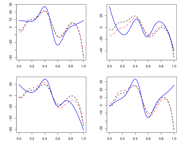
Figure 1: True derivative curves and the corresponding estimates obtained by FPCA and DPCA, for four randomly selected sparsely sampled trajectories generated in Simulation A (sparse designs) with $\sigma=2$. Each of the four panels represents an individual derivative trajectory and consists of the true underlying derivative (solid), the derivative estimates by FPCA (dashed) and by DPCA (dash-dot).

The results for Simulation B for dense designs are shown in Table 2. We found that under both small ($\sigma=1$) and large ($\sigma=2$) measurement errors, the proposed DPCA clearly outperforms the other three methods in terms of RMISE. The runner-up among the other methods is FPCA, but it was highly unstable for more than five components. Performance for all methods was better with smaller measurement errors ($\sigma=1$), due to the fact that it is particularly difficult to infer derivatives in situations with large measurement errors. Also, unsurprisingly, under the same level of measurement errors, all methods achieve smaller RMISE for dense designs, compared to their respective performance under sparse designs. This shows that DPCA has a significant advantage over FPCA in the dense setting.

Table 2: Relative mean integrated squared errors (RMISE) for Simulation B, dense designs, with error standard deviation $\sigma=1$ or $\sigma=2$. We report the mean of the RMISE based on 400 Monte Carlo repeats, where the standard deviations are all between 0.01 and 0.02 for all except LOCAL. For LOCAL, the derivative of each curve is estimated individually using local quadratic kernel smoothing; for SMOOTH-DQ, the derivative of each curve is obtained via smoothing of the difference quotients of the observed measurements. The first 5 columns correspond to FPCA and DPCA using different numbers of fixed $K$; the 6th column corresponds to selecting $K$ according to FVE, with the mean of the selected $K$ in brackets.

$\sigma=1$	$K=1$	$K=2$	$K=3$	$K=4$	$K=5$	FVE	LOCAL	SMOOTH-DQ
FPCA	0.51	0.42	0.27	0.2	0.16	0.16 (5.0)	0.23	0.65
DPCA	0.32	0.22	0.16	0.13	0.08	0.13 (3.9)
$\sigma=2$	$K=1$	$K=2$	$K=3$	$K=4$	$K=5$	FVE	LOCAL	SMOOTH-DQ
FPCA	0.51	0.43	0.29	0.27	0.26	0.26 (5.0)	0.51	0.76
DPCA	0.34	0.26	0.22	0.19	0.18	0.20 (3.9)

6 Applications

6.1 Modeling Derivatives of Tammar Wallaby Body Length Data

We applied the proposed DPCA for derivative estimation to the Wallaby growth data, which can be found at http://www.statsci.org/data/oz/wallaby.html, from the Australian Dataset and Story Library (OzDASL). This dataset includes body length measurements for 36 tammar wallabies (Macropus eugenii), longitudinally taken and collected from wallabies in their early age. A detailed introduction of the dataset is given by Mallon (1994). To gain a better understanding of the growth pattern of wallabies, we investigated the dynamics of their body length growth by estimating the derivatives of their growth trajectories.

One main difficulty is that the body length measurements are very sparse, irregular, and fragmentary, as shown in Figure 2, making these data a good test case to reveal the difficulties in recovering derivatives from sparse longitudinal designs. The 36 wallabies included in the dataset had their body length measured from 1 to 12 times per subject, with a median of 3.5 measurements per subject.

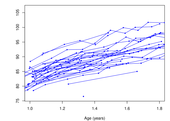
Figure 2: The trajectory spaghetti plot of body length growth for 36 wallabies. The recorded measurements over time for each wallaby are quite sparse, with measurement counts ranging from 1 to 12.

Aiming at a number of components with 90% FVE leads to inclusion of the first $K=3$ derivative eigenfunctions. The estimated first derivative of the mean function, eigenfunctions of the original growth trajectories, and those of the derivatives by the proposed approach are shown in Figure 3. The average dynamic changes in body length are represented by the mean derivative function (upper left panel), which exhibits a monotonically decreasing trend, from greater than 25 cm/yr at age 1 to less than 10 cm/yr at age 1.8, where the decline rate of the mean derivative function becomes generally slower as age increases. The first eigenfunction (solid) of the trajectories reflects overall body length at different ages, the second eigenfunction (dashed) characterizes a contrast in length between early and late stages, and the third eigenfunction (dotted) corresponds to a contrast between a period around 1.5 years and the other stages (upper right panel).

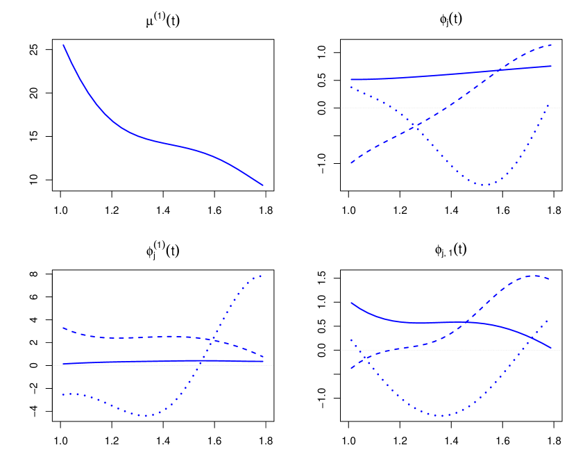
Figure 3: Upper left: estimated mean derivative function of the body length for wallabies; upper right: estimated first three eigenfunctions of body length trajectories from FPCA, explaining $97\%$, $2.4\%$, and 0.59% of overall variance in the trajectories, respectively; lower left: estimated derivatives of the eigenfunctions of body length trajectories in the upper right panel; lower right: estimated eigenfunctions for derivatives from DPCA, explaining 62.8%, 26.1%, and 10.9% of overall variance in the derivatives. First, second and third eigenfunctions are denoted by solid, dashed, and dotted lines, respectively.

The primary mode of dynamic changes in body length, as reflected by the first eigenfunction of the derivatives in the lower right panel (solid) of Figure 3, represents the overall speed of growth which has a decreasing trend as wallabies get older. The second mode of dynamic variation is determined by the second eigenfunction of the derivatives (dashed) that mainly contrasts dynamic variation during young age with that of late ages. The third eigenfunction of the derivatives (dotted) emphasizes growth variation around age 1.38 and stands for a contrast of growth speed between middle age and early/late ages. The eigenfunctions of derivatives are seen to clearly differ from the derivatives of the eigenfunctions (lower left panel) of the trajectories themselves, and are well interpretable.

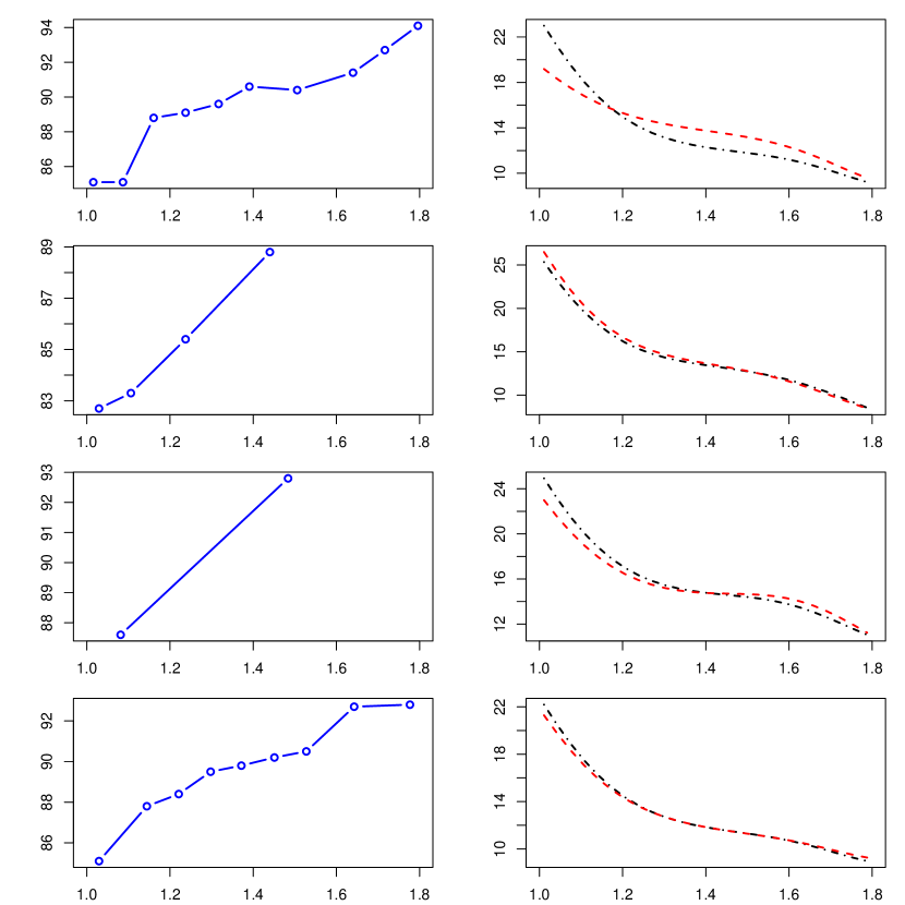
Figure 4: Data and corresponding estimated derivatives of body length growth for four randomly selected wallabies. Left panels: original body length data connected by lines; right panels: the derivative estimates obtained by FPCA (dash-dot) and the proposed DPCA (dashed).

Figure 4 exhibits the trajectories and corresponding derivatives estimates by FPCA and DPCA for four randomly selected wallabies, where the derivatives were constructed using $K=3$ components, the smallest number that leads to 90% FVE. Here the DPC-derived derivatives are seen to be reflective of the data dynamics.

6.2 Classifying Wheat Spectra

As a second example we applied the proposed DPCA to the near infrared (NIR) spectral dataset of wheat, which consists of NIR spectra of 87 wheat samples with known protein content. The spectra of the samples were measured by diffuse reflectance from 1100 to 2500 nm with 10 nm intervals, as displayed in the left panel of Figure 5. For these data, it is of interest to investigate whether the spectrum of a wheat sample can be utilized to predict its protein content. Protein content is an important factor for wheat storage, and higher protein contents may increase the market price. For a more detailed description of these data, we refer to Kalivas (1997). Functional data analysis of these data has been studied by various authors, including Reiss and Ogden (2007), and Delaigle and Hall (2012).

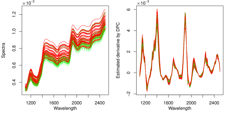
Figure 5: Left panel: observed trajectories for the NIR spectra of 87 wheat samples (high: solid; low: dashed). Right panel: estimated derivatives of the wheat sample NIR spectra trajectories using DPCA, based on the first four DPCs.

As can be seen from the left panel of Figure 5, the wheat samples are found to exhibit very similar spectral patterns: the overall trend for all trajectories is increasing, with three major local peaks appearing at wavelengths around 1200 nm, 1450 nm, and 1950 nm. The trajectories are almost parallel to each other, with only minor differences in the overall level. The response to be predicted is the protein content of a wheat sample, which is grouped into categories— high if a sample has more than 11.3% protein, and low if less than 11.3%. From the trajectory graphs it appears to be a non-trivial problem to classify the wheat samples, since the trajectories corresponding to the high protein wheats are highly spread out vertically and overlap on the lower side with those corresponding to the low group.

It has been suggested (Delaigle and Hall 2012) that derivatives of wheat spectra are particularly suitable for classification of these spectra. We therefore applied the proposed DPCA for the fitting of these spectra and this led to the estimated derivatives of wheat spectra shown in the right panel of Figure 5. These fits are based on including the first four DPCs, which collectively explain 99.2% of the total variation in the derivatives.

Table 3: The mean fraction of misclassified samples, by randomly taking 30 samples as the training set and the rest 57 samples as the test set. The standard deviations of the misclassification rates are between 0.05 and 0.07. Classification models were built with different numbers of FPCs and DPCs, respectively. The first 8 columns are for fixed $K$ ranging from 1 to 8; the last column corresponds to selecting $K$ by 5-fold CV, with the mean of the chosen $K$ in brackets.

	$K=1$	$K=2$	$K=3$	$K=4$	$K=5$	$K=6$	$K=7$	$K=8$	CV
FPCA	0.274	0.253	0.267	0.284	0.293	0.280	0.273	0.280	0.282 (3.5)
DPCA	0.503	0.238	0.249	0.259	0.274	0.284	0.294	0.299	0.264 (3.5)

For a comparative evaluation of the performance of using FPCA as opposed to DPCA for the purpose of classifying protein contents of wheat samples, we used a logistic regression with one to eight FPCs or DPCs as predictors. We randomly drew 30 samples as training sets and 57 as test sets, repeated this 500 times, and report the average misclassification rates for the test sets in Table 3, in which the first eight columns stand for using a fixed number of components, and the last column for selecting $K$ based on 5-fold cross-validation (CV), minimizing the misclassification rate. We found that the DPCA-based classifier outperforms the FPCA-based classifier if two to five predictor components were included, or if CV was used to select $K$. The minimal misclassification rate is 23.8% using two components, while the best FPCA-based misclassification rate is 25.3%. The poor performance of DPCA when $K=1$ indicates the first DPC does not provide information for classification alone, while the second DPC may be a superior predictor of interest. While there are some improvements in the misclassification rates when using DPCs, they are relatively small in terms of misclassification error.

Appendix

Appendix A.1 Estimating Mean Function and Eigenfunctions For Derivatives

To implement (12), one needs to obtain $\mu^{(1)}(t)$, the first order derivative of the mean function. Let $N=\sum_{i=1}^{n}N_{i}$, $w_{i}=N^{-1}$, and $v_{i}=[\sum_{i=1}^{n}N_{i}(N_{i}-1)]^{-1}$. Applying local quadratic smoothing to a pooled scatterplot, one can aggregate the observed measurements from all sample trajectories and minimize

$$\sum_{i=1}^{n}w_{i}\sum_{j=1}^{N_{i}}K_{h_{\mu}}\Big{(}\frac{T_{ij}-t}{h_{\mu,1}}\Big{)}\Big{[}Y_{ij}-\sum_{p=0}^{2}\alpha_{p}(T_{ij}-t)^{p}\Big{]}^{2}$$ (25)

with respect to $\alpha_{p}$, $p=0,1,2$. The minimizer $\hat{\alpha}_{1}(t)$ is the estimate of $\mu^{(1)}(t)$, $\hat{\mu}^{(1)}(t)=\hat{\alpha}_{1}(t)$ (Liu and Müller (2009), equation (5)). Here $K_{h}(x)=h^{-1}K(x/h)$, $K(\cdot)$ is a univariate density function, and $h_{\mu}$ is a positive bandwidth that can be chosen by GCV in practical implementation.

In order to estimate the eigenfunctions $\phi_{k,1}$ of the derivatives $X^{(1)}$, we proceed by first estimating the covariance kernel $G_{1}(s,t)$ (in (4) with $\nu=1$), followed by a spectral decomposition of the estimated kernel. According to (8), $\displaystyle G_{1}(s,t)=G^{(1,1)}(s,t)$ for the case $\nu=1$; this can be estimated by a two-dimensional kernel smoother targeting the mixed partial derivatives of the covariance function. Specifically, we aim at minimizing

$$\sum_{i=1}^{n}v_{i}\sum_{1\leq j\neq l\leq N_{i}}K_{h_{G}}(T_{ij}-t)K_{h_{G}}(T_{il}-s)\Big{[}G_{i}(T_{ij},T_{il})-\sum_{0\leq p+q\leq 3}\alpha_{pq}(T_{ij}-t)^{p}(T_{il}-s)^{q}\Big{]}^{2},$$ (26)

with respect to $\alpha_{pq}$ for $0\leq p+q\leq 3$, and set $\hat{G}^{(1,1)}(s,t)$ to the minimizer $\hat{\alpha}_{11}(s,t)$. For theoretical derivations we adopt this direct estimate of $\hat{G}^{(1,1)}(s,t)$, while in practical implementation it has been found to be more convenient to first obtain $\hat{G}^{(1,0)}(s,t)$ and then to apply a local linear smoother on the second direction, which also led to better stability and boundary behavior.

After obtaining estimates $\hat{G}^{(1,1)}$ of $G^{(1,1)}$, eigenfunctions and eigenvalues of the derivatives can be estimated by the spectral decomposition of $\hat{G}^{(1,1)}(s,t)$,

$$\hat{G}^{(1,1)}(s,t)=\sum_{k=1}^{\infty}\hat{\lambda}_{k,1}\hat{\phi}_{k,\nu}(s)\hat{\phi}_{k,1}(t).$$

Appendix A.2 Assumptions, Proofs and Auxiliary Results

For our results we require assumptions (A1)–(A8), paralleling assumptions (A1)–(A2), (B1)–(B4), (C1c)–(C2c), and (D1c)–(D2c) in Zhang and Wang (2016). Denote the inner product on $L^{2}(\mathcal{T})$ by $\langle x,y\rangle$.

1. $K(\cdot)$ is a symmetric probability density function on $[-1,1]$ and is Lipschitz continuous: There exists $0<L<\infty$ such that $|K(u)-K(v)|\leq L|u-v|$ for any $u,v\in[0,1]$.

2. $\{T_{ij}:i=1,\dots,n,\,j=1,\dots,N_{i}\}$ are i.i.d. copies of a random variable $T$ defined on $\mathcal{T}$, and $N_{i}$ are regarded as fixed. The density $f(\cdot)$ of $T$ is bounded below and above,

   $$0<m_{f}\leq\min_{t\in\mathcal{T}}f(t)\leq\max_{t\in\mathcal{T}}f(t)\leq M_{f}<\infty.$$

   Furthermore $f^{(2)}$, the second derivative of $f(\cdot)$, is bounded.

3. $X$, $e$, and $T$ are independent.

4. $\mu^{(3)}(t)$ and $\partial^{4}G(s,t)/\partial^{p}\partial^{4-p}$ exist and are bounded on $\mathcal{T}$ and $\mathcal{T}\times\mathcal{T}$, respectively, for $p=0,\dots,4$.

5. $h_{\mu}\rightarrow 0$ and $\log(n)\sum_{i=1}^{n}N_{i}w_{i}^{2}/h_{\mu}\rightarrow 0$.

6. For some $\alpha>2$, $E(\sup_{t\in\mathcal{T}}|X(t)-\mu(t)|^{\alpha})<\infty$, $E(|e|^{\alpha})<\infty$, and

   $$n\left[\sum_{i=1}^{n}N_{i}w_{i}^{2}h_{\mu}+\sum_{i=1}^{n}N_{i}(N_{i}-1)w_{i}^{2}h_{\mu}^{2}\right]\left[\frac{\log(n)}{n}\right]^{2/\alpha-1}\rightarrow\infty.$$

7. $h_{G}\rightarrow 0$, $\log(n)\sum_{i=1}^{n}N_{i}(N_{i}-1)v_{i}^{2}/h_{G}^{2}\rightarrow 0$.

8. For some $\beta>2$, $E(\sup_{t\in\mathcal{T}}|X(t)-\mu(t)|^{2\beta})<\infty$, $E(|e|^{2\beta})<\infty$, and

   $$n\bigg{[} \sum_{i=1}^{n}N_{i}(N_{i}-1)v_{i}^{2}h_{G}^{2}+\sum_{i=1}^{n}N_{i}(N_{i}-1)(N_{i}-2)v_{i}^{2}h_{G}^{3}$$

   $$+\sum_{i=1}^{n}N_{i}(N_{i}-1)(N_{i}-2)(N_{i}-3)v_{i}^{2}h_{G}^{4}\bigg{]}\left[\frac{\log(n)}{n}\right]^{2/\beta-1}\rightarrow\infty.$$

9. For any $k=1,2,\dots$, there exists $J=J(k)<\infty$ such that $\langle\phi_{j}^{(1)},\phi_{k,1}\rangle$ = 0 for all $j>J$.

Note that (A9) holds for any infinite-dimensional processes where the eigenfunctions correspond to the Fourier basis or Legendre basis.

Proof of Theorem 1:.

We first prove the rate of convergence in the supremum norm for $\hat{\mu}^{(1)}$ to $\mu^{(1)}$, following the proof of Theorem 5.1 in Zhang and Wang (2016). Denote for $r=0,\dots,4$

$$S_{r}=\sum_{i=1}^{n}w_{i}\sum_{j=1}^{N_{i}}K_{h_{\mu}}(T_{ij}-t)\left(\frac{T_{ij}-t}{h_{\mu}}\right)^{r},\quad R_{r}=\sum_{i=1}^{n}w_{i}\sum_{j=1}^{N_{i}}K_{h_{\mu}}(T_{ij}-t)\left(\frac{T_{ij}-t}{h_{\mu}}\right)^{r}Y_{ij},$$

$$\mathbf{S}=\left[\begin{array}[]{ccc}S_{0}&S_{1}&S_{2}\\ S_{1}&S_{2}&S_{3}\\ S_{2}&S_{3}&S_{4}\end{array}\right],\quad\left[\begin{array}[]{c}\hat{\alpha}_{0}\\ h_{\mu}\hat{\alpha}_{1}\\ h_{\mu}^{2}\hat{\alpha}_{2}\end{array}\right]=\mathbf{S}^{-1}\left[\begin{array}[]{c}R_{0}\\ R_{1}\\ R_{2}\end{array}\right].$$

For a square matrix $\mathbf{A}$ let $|\mathbf{A}|$ denote its determinant and $[\mathbf{A}]_{a,b}$ denote the $(a,b)$th entry of $\mathbf{A}$. Then $h_{\mu}\hat{\mu}^{(1)}(t)=h_{\mu}\hat{\alpha}_{0}=|\mathbf{S}|^{-1}(C_{12}R_{0}+C_{22}R_{1}+C_{32}R_{2})$ by Cramer’s rule (Lang 1987), where

$$C_{12}=\left|\begin{array}[]{cc}S_{1}&S_{3}\\ S_{2}&S_{4}\end{array}\right|,\quad C_{22}=\left|\begin{array}[]{cc}S_{0}&S_{2}\\ S_{2}&S_{4}\end{array}\right|,\quad C_{23}=\left|\begin{array}[]{cc}S_{0}&S_{2}\\ S_{1}&S_{3}\end{array}\right|$$

are the cofactors for $[\mathbf{S}]_{1,2}$, $[\mathbf{S}]_{2,2}$, and $[\mathbf{S}]_{3,2}$, respectively. Then

$$h_{\mu}(\hat{\alpha}_{1} -\mu^{(1)}(t))=|\mathbf{S}|^{-1}\{\left[C_{12}R_{0}+C_{22}R_{1}+C_{32}R_{2}\right]$$

$$\hskip 60.00009pt-\left[C_{12}S_{0}+C_{22}S_{1}+C_{32}S_{2}\right]$$

$$\hskip 60.00009pt-\left[C_{12}S_{2}+C_{22}S_{3}+C_{32}S_{4}\right]\mu^{(2)}(t)h_{\mu}^{2}$$

$$\hskip 60.00009pt-\left[C_{12}S_{1}+C_{22}S_{2}+C_{32}S_{3}\right]\mu^{(1)}(t)h_{\mu}\}$$

$$=|\mathbf{S}|^{-1}\sum_{p=0}^{2}C_{(p+1),2}(R_{p}-S_{p}-\mu^{(1)}(t)h_{\mu}S_{p+1}-\mu^{(2)}(t)h_{\mu}S_{p+2})$$

$$=|\mathbf{S}|^{-1}\sum_{p=0}^{2}C_{(p+1),2}\bigg{[}\sum_{i=1}^{n}w_{i}\sum_{j=1}^{N_{i}}K_{h_{\mu}}(T_{ij}-t)\left(\frac{T_{ij}-t}{h_{\mu}}\right)^{p}\delta_{ij}$$

$$\quad+\sum_{i=1}^{n}w_{i}\sum_{j=1}^{N_{i}}K_{h_{\mu}}(T_{ij}-t)\left(\frac{T_{ij}-t}{h_{\mu}}\right)^{p}h_{\mu}^{3}\mu^{(3)}(z)\bigg{]}$$

$$=|\mathbf{S}|^{-1}\sum_{p=0}^{2}C_{(p+1),2}\bigg{[}O\bigg{(}\bigg{\{}\log(n)\bigg{[}\sum_{i=1}^{n}N_{i}w_{i}^{2}h_{\mu}+\sum_{i=1}^{n}N_{i}(N_{i}-1)w_{i}^{2}h_{\mu}^{2}\bigg{]}\bigg{\}}^{1/2}\bigg{)}+O(h_{\mu}^{3})\bigg{]}\quad\text{a.s.};$$

here the first equality is due to the properties of determinants, the third is due to Taylor’s theorem, and the last is due to Lemma 5 in Zhang and Wang (2016), (A1), and (A4), where the $O(\cdot)$ terms are seen to be uniform in $t\in\mathcal{T}$. By Theorem 5.1 in Zhang and Wang (2016), the $S_{r}$ converge almost surely to their respective means in supremum norm and are thus bounded almost surely for $r=0,\dots,4$, so that $C_{(p+1),2}$ is bounded almost surely for $p=0,1,2$. Then $|\mathbf{S}|^{-1}$ is bounded away from 0 by the almost sure supremum convergence of $S_{r}$ and Slutsky’s theorem. Therefore the convergence rate for $\hat{\mu}^{(1)}$ is

$$\sup_{t\in\mathcal{T}}|\hat{\mu}^{(1)}(t)-\mu^{(1)}(t)|=O\bigg{(}\bigg{\{}\log(n)\bigg{[}\sum_{i=1}^{n}N_{i}w_{i}^{2}/h_{\mu}+\sum_{i=1}^{n}N_{i}(N_{i}-1)w_{i}^{2}\bigg{]}\bigg{\}}^{1/2}+h_{\mu}^{2}\bigg{)}\quad\text{a.s.}$$

The rate (17) then follows by replacing $N_{i}$ by $N_{0}$ in the sparse case where $N_{i}\leq N_{0}<\infty$, and by $m$ in the dense case where $m\rightarrow\infty$, respectively.

The supremum convergence rate for $\hat{G}^{(1,1)}$ can be proven similarly, following the development of Theorem 5.2 in Zhang and Wang (2016). The supremum convergence rate for $\hat{\phi}_{k,1}$ is a direct consequence of that for $\hat{G}^{(1,1)}$; see the proof of Theorem 2 in Yao et al. (2005). ∎

Proof of Theorem 2:.

For a vector $\mathbf{v}$, let $\left\lVert\mathbf{v}\right\rVert$ be the vector $L^{2}$ norm and, for a square matrix $\mathbf{A}$, let $\left\lVert\mathbf{A}\right\rVert=\sup_{\mathbf{v}\neq 0}\left\lVert\mathbf{A}\mathbf{v}\right\rVert/\left\lVert\mathbf{v}\right\rVert$ be the matrix operator norm. We start with a proposition that follows from the proof of Corollary 1 in Yao et al. (2005), our Theorem 1, and a lemma from Facer and Müller (2003).

Proposition 1.

Under the conditions of Theorem 1,

$$\sup_{t\in\mathcal{T}}|\hat{\mu}(t)-\mu(t)| =O(a_{n})\quad\text{a.s.},$$

$$\sup_{s,t\in\mathcal{T}}|\hat{G}(s,t)-G(s,t)| =O(a_{n}+b_{n})\quad\text{a.s.},$$

$$\sup_{s,t\in\mathcal{T}}|\hat{G}^{(1,0)}(s,t)-G^{(1,0)}(s,t)| =O(a_{n}+b_{n})\quad\text{a.s.},$$

$$|\hat{\sigma}^{2}-\sigma^{2}| =O(a_{n}+b_{n})\quad\text{a.s.}$$

Lemma 1 (Lemma A.3, Facer and Müller (2003)).

Let $\mathbf{A}\in\mathcal{M}_{m}(\mathbb{R})$ be invertible. For all $\mathbf{B}\in\mathcal{M}_{m}(\mathbb{R})$ such that

$$\|\mathbf{A}-\mathbf{B}\|<\frac{1}{2\|\mathbf{A}^{-1}\|},$$

$\mathbf{B}^{-1}$ always exists and there exists a constant $0<c<\infty$ such that

$$\|\mathbf{B}^{-1}-\mathbf{A}^{-1}\|\leq c\|\mathbf{A}^{-1}\|^{2}\|\mathbf{A}-\mathbf{B}\|.$$

To prove the first statement of Theorem 2, note

$$|\hat{\xi}_{ik,1}-\tilde{\xi}_{ik,1}| =\hat{\bm{\zeta}}_{ik}^{T}\hat{\bm{\Sigma}}_{\mathbf{Y}_{i}}^{-1}(\mathbf{Y}_{i}-\hat{\bm{\mu}}_{i})-\bm{\zeta}_{ik}^{T}\bm{\Sigma}_{\mathbf{Y}_{i}}^{-1}(\mathbf{Y}_{i}-\bm{\mu}_{i})$$

$$=\hat{\bm{\zeta}}_{ik}^{T}(\hat{\bm{\Sigma}}_{\mathbf{Y}_{i}}^{-1}-\bm{\Sigma}_{\mathbf{Y}_{i}}^{-1})(\mathbf{Y}_{i}-\hat{\bm{\mu}}_{i})+(\hat{\bm{\zeta}}_{ik}-\bm{\zeta}_{ik})^{T}\bm{\Sigma}_{\mathbf{Y}_{i}}^{-1}(\mathbf{Y}_{i}-\hat{\bm{\mu}}_{i})$$

$$\quad+\hat{\bm{\zeta}}_{ik}\bm{\Sigma}_{\mathbf{Y}_{i}}^{-1}(\bm{\mu}_{i}-\hat{\bm{\mu}}_{i})-(\hat{\bm{\zeta}}_{ik}-\bm{\zeta}_{ik})^{T}\bm{\Sigma}_{\mathbf{Y}_{i}}^{-1}(\bm{\mu}_{i}-\hat{\bm{\mu}}_{i})$$

$$\leq\left\lVert\hat{\bm{\zeta}}_{ik}\right\rVert\left\lVert\hat{\bm{\Sigma}}_{\mathbf{Y}_{i}}^{-1}-\bm{\Sigma}_{\mathbf{Y}_{i}}^{-1}\right\rVert\left\lVert\mathbf{Y}_{i}-\hat{\bm{\mu}}_{i}\right\rVert+\left\lVert\hat{\bm{\zeta}}_{ik}-\bm{\zeta}_{ik}\right\rVert\left\lVert\bm{\Sigma}_{\mathbf{Y}_{i}}^{-1}\right\rVert\left\lVert\mathbf{Y}_{i}-\hat{\bm{\mu}}_{i}\right\rVert$$

$$\quad+\left\lVert\hat{\bm{\zeta}}_{ik}\right\rVert\left\lVert\bm{\Sigma}_{\mathbf{Y}_{i}}^{-1}\right\rVert\left\lVert\bm{\mu}_{i}-\hat{\bm{\mu}}_{i}\right\rVert+\left\lVert\hat{\bm{\zeta}}_{ik}-\bm{\zeta}_{ik}\right\rVert\left\lVert\bm{\Sigma}_{\mathbf{Y}_{i}}^{-1}\right\rVert\left\lVert\bm{\mu}_{i}-\hat{\bm{\mu}}_{i}\right\rVert.$$ (27)

We bound each term as follows, using the notation $\lesssim$ to indicate that the left hand side is smaller than a constant multiple of the right hand side. We have $\left\lVert\hat{\bm{\zeta}}_{ik}-\bm{\zeta}_{ik}\right\rVert\leq\sqrt{N_{i}}\sup_{j}|\hat{\zeta}_{ikj}-\zeta_{ikj}|$, and

$$\sup_{j}|\hat{\zeta}_{ikj}-\zeta_{ikj}| =\sup_{j}|\int\hat{G}^{(1,0)}(s,T_{ij})\hat{\phi}_{k,1}(s)ds-\int G^{(1,0)}(s,T_{ij})\phi_{k,1}(s)ds|$$

$$\leq\sup_{t\in\mathcal{T}}|\int[\hat{G}^{(1,0)}(s,t)-G^{(1,0)}(s,t)]\hat{\phi}_{k,1}(s)ds|+\sup_{t\in\mathcal{T}}\int G^{(1,0)}(s,t)[\hat{\phi}_{k,1}(s)-\phi_{k,1}(s)]ds$$

$$\lesssim\sup_{t\in\mathcal{T}}\left\{\int[\hat{G}^{(1,0)}(s,t)-G^{(1,0)}(s,t)]^{2}ds\right\}^{1/2}+\sup_{s,t\in\mathcal{T}}|G^{(1,0)}(s,t)|\sup_{t\in\mathcal{T}}|\hat{\phi}_{k,1}(t)-\phi_{k,1}(t)|$$

$$=O(\sup_{t\in\mathcal{T}}|\hat{G}^{(1,0)}-G^{(1,0)}|)+O(\sup_{t\in\mathcal{T}}|\hat{\phi}_{k,1}(t)-\phi_{k,1}(t)|),$$

where the last equality is due to (A4). By Proposition 1 we have

$$\left\lVert\hat{\bm{\zeta}}_{ik}-\bm{\zeta}_{ik}\right\rVert=O(\sqrt{N_{i}}(a_{n}+b_{n}))\quad\text{a.s.}$$ (28)

Similarly, $\sup_{j}|\zeta_{ikj}|\leq\sup_{t\in\mathcal{T}}|G^{(1,0)}(s,t)\phi_{k,1}(s)ds|=O(1)$. Take $\bm{\epsilon}_{i}=(\varepsilon_{i1},\dots,\varepsilon_{im})^{T}$ and $\mathbf{X}_{i}=(X(T_{i1}),\dots,X(T_{im}))^{T}$. Then

$$\left\lVert\hat{\bm{\zeta}}_{ik}\right\rVert \leq\left\lVert\bm{\zeta}_{ik}\right\rVert+\left\lVert\hat{\bm{\zeta}}_{ik}-\bm{\zeta}_{ik}\right\rVert=\sqrt{N_{i}}[O(1)+O(a_{n}+b_{n})]=O(\sqrt{N_{i}})\quad\text{a.s.},$$ (29)

$$\left\lVert\bm{\mu}_{i}-\hat{\bm{\mu}}_{i}\right\rVert \leq\sqrt{N_{i}}\sup_{t\in\mathcal{T}}|\hat{\mu}(t)-\mu(t)|=O(\sqrt{N_{i}}a_{n})\quad\text{a.s.},$$ (30)

$$\left\lVert\mathbf{Y}_{i}-\hat{\bm{\mu}}_{i}\right\rVert \leq\left\lVert\bm{\epsilon}_{i}\right\rVert+\left\lVert\mathbf{X}_{i}-\bm{\mu}_{i}\right\rVert+\left\lVert\hat{\bm{\mu}}_{i}-\bm{\mu}_{i}\right\rVert=O_{p}(\sqrt{N_{i}})$$ (31)

where (31) is by the Weak Law of Large Numbers. From the definition of $\bm{\Sigma}_{\mathbf{Y}_{i}}$ we have $\left\lVert\bm{\Sigma}_{\mathbf{Y}_{i}}^{-1}\right\rVert\leq\sigma^{-2}$. Then

$$\left\lVert\hat{\bm{\Sigma}}_{\mathbf{Y}_{i}}^{-1}-\bm{\Sigma}_{\mathbf{Y}_{i}}^{-1}\right\rVert \leq c\sigma^{-4}\left\lVert\hat{\bm{\Sigma}}_{\mathbf{Y}_{i}}-\bm{\Sigma}_{\mathbf{Y}_{i}}\right\rVert$$

$$\leq c\sigma^{-4}N_{i}\sup_{a,b}|[\hat{\bm{\Sigma}}_{\mathbf{Y}_{i}}]_{ab}-[\bm{\Sigma}_{\mathbf{Y}_{i}}]_{ab}|$$

$$=O(N_{i}(a_{n}+b_{n}))\quad\text{a.s.},$$ (32)

where the first inequality is by Lemma 1, the second by a property of matrix operator norm, and the last relies on $\sup_{a,b}|[\hat{\bm{\Sigma}}_{\mathbf{Y}_{i}}]_{ab}-[\bm{\Sigma}_{\mathbf{Y}_{i}}]_{ab}|\leq|\hat{\sigma}^{2}-\sigma^{2}|+\sup_{s,t\in\mathcal{T}}|\hat{G}(s,t)-G(s,t)|=O(a_{n}+b_{n})$ a.s. by Proposition 1. Combining (27)–(32) leads to the proof of the first statement.

Under the dense assumption we have $N_{i}=m\rightarrow\infty$. Since $\zeta_{ikl}=\int_{\mathcal{T}}G^{(1,0)}(s,T_{il})\phi_{k,1}(s)ds=\int_{\mathcal{T}}\sum_{j=1}^{\infty}\lambda_{j}\phi_{j}^{(1)}(s)\phi_{j}(T_{il})\phi_{k,1}(s)ds=\sum_{j=1}^{\infty}\lambda_{j}\langle\phi_{j}^{(1)},\phi_{k,1}\rangle\phi_{j}(T_{il})$ for $l=1,\dots,m$, under (A9) we have $\bm{\zeta}_{ik}=\sum_{j=1}^{J}\lambda_{j}\langle\phi_{j}^{(1)},\phi_{k,1}\rangle\bm{\phi}_{j}$, where we take $\bm{\phi}_{j}=(\phi_{j}(T_{i1}),\dots,\phi_{j}(T_{im}))^{T}$. Then

$$\tilde{\xi}_{ik,1} =\bm{\zeta}_{ik}^{T}\bm{\Sigma}_{\mathbf{Y}_{i}}^{-1}(\mathbf{Y}_{i}-\bm{\mu}_{i})=\sum_{j=1}^{J}\lambda_{j}\langle\phi_{j}^{(1)},\phi_{k,1}\rangle\bm{\phi}_{j}^{T}\bm{\Sigma}_{\mathbf{Y}_{i}}^{-1}(\mathbf{Y}_{i}-\bm{\mu}_{i}),$$

$$\xi_{ik,1} =\langle X^{(1)},\phi_{k,1}\rangle=\langle\sum_{j=1}^{\infty}\xi_{ij}\phi_{j}^{(1)},\phi_{k,1}\rangle=\sum_{j=1}^{J}\xi_{ij}\langle\phi_{j}^{(1)},\phi_{k,1}\rangle,$$

so it suffices to prove for $j=1,\dots,J$,

$$\bm{\phi}_{j}^{T}\bm{\Sigma}_{\mathbf{Y}_{i}}^{-1}(\mathbf{Y}_{i}-\bm{\mu}_{i})=\xi_{ij}/\lambda_{j}+O_{p}(m^{-1/2}).$$ (33)

Under joint Gaussianity of $(X,\epsilon)$, $E(\xi_{ij}\mid\mathbf{Y}_{i})=\lambda_{j}\bm{\phi}_{j}^{T}\bm{\Sigma}_{\mathbf{Y}_{i}}^{-1}(\mathbf{Y}_{i}-\bm{\mu}_{i})$ is the posterior mean of $\langle X_{i},\phi_{j}\rangle$ given the observations $\mathbf{Y}_{i}$. By the convergence results for nonparametric posterior distributions as in Theorem 3 of Shen (2002), we have

$$|E(\xi_{ij}\mid\mathbf{Y}_{i})-\xi_{ij}|=O_{p}(m^{-1/2})$$

as $m\rightarrow\infty$, which implies (33) and therefore the second statement of Theorem 2.

∎

Proof of Theorem 3:.

For all $i=1,2,\ldots$ and any fixed $K$,

$$\sup_{t\in\mathcal{T}}|\hat{X}^{(1)}_{i,K}(t)-\tilde{X}^{(1)}_{i,K}(t)| =\sup_{t\in\mathcal{T}}|\sum_{k=1}^{K}(\hat{\xi}_{ik,1}-\tilde{\xi}_{ik,1})\hat{\phi}_{k,1}(t)+\sum_{k=1}^{K}\tilde{\xi}_{ik,1}(\hat{\phi}_{k,1}(t)-\phi_{k,1}(t))|$$

$$=\sum_{k=1}^{K}|\hat{\xi}_{ik,1}-\tilde{\xi}_{ik,1}|O_{p}(1)+\sum_{k=1}^{K}|\tilde{\xi}_{ik,1}|\,\sup_{t\in\mathcal{T}}|\hat{\phi}_{k,1}(t)-\phi_{k,1}(t)|$$

$$=O_{p}(N_{i}^{2}(a_{n}+b_{n})+(a_{n}+b_{n}))=O_{p}(N_{i}^{2}(a_{n}+b_{n})).$$

A similar rate for $\sup_{t\in\mathcal{T}}|\hat{X}^{(1)}_{i,K}(t)-X^{(1)}_{i,K}(t)|$ in the dense case is obtained by applying Theorem 2 and repeating the previous argument. ∎

REFERENCES

• Bapna et al. (2008) Bapna, R., Jank, W. and Shmueli, G. (2008). Price formation and its dynamics in online auctions. Decision Support Systems 44, 641–656.
• de Boor (1972) de Boor, C. (1972). On calculating with $B$-splines. Journal of Approximation Theory 6, 50–62.
• Chambers and Hastie (1991) Chambers, J. M. and Hastie, T. (eds.) (1991). Statistical Models in S. Pacific Grove: Duxbury Press.
• Delaigle and Hall (2012) Delaigle, A. and Hall, P. (2012). Achieving near perfect classification for functional data. Journal of the Royal Statistical Society: Series B (Statistical Methodology) 74, 267–286.
• Facer and Müller (2003) Facer, M. and Müller, H.-G. (2003). Nonparametric estimation of the peak location in a response surface. Journal of Multivariate Analysis 87, 191–217.
• Fan and Gijbels (1996) Fan, J. and Gijbels, I. (1996). Local Polynomial Modelling and its Applications. London: Chapman & Hall.
• Gasser and Müller (1984) Gasser, T. and Müller, H.-G. (1984). Estimating regression functions and their derivatives by the kernel method. Scandinavian Journal of Statistics 11, 171–185.
• Grenander (1950) Grenander, U. (1950). Stochastic processes and statistical inference. Arkiv för Matematik 1, 195–277.
• Jank and Shmueli (2005) Jank, W. and Shmueli, G. (2005). Profiling price dynamics in online auctions using curve clustering. Technical Report. SSRN eLibrary.
• Kalivas (1997) Kalivas, J. H. (1997). Two data sets of near infrared spectra. Chemometrics and Intelligent Laboratory Systems 37, 255–259.
• Lang (1987) Lang, S. (1987). Linear Algebra. New York: Springer.
• Liu and Müller (2009) Liu, B. and Müller, H.-G. (2009). Estimating derivatives for samples of sparsely observed functions, with application to on-line auction dynamics. Journal of the American Statistical Association 104, 704–714.
• Mallon (1994) Mallon, G. (1994). Mixed linear models and applications. Ph.D. thesis. University of Queensland, Department of Mathematics.
• Müller and Yao (2010) Müller, H.-G. and Yao, F. (2010). Empirical dynamics for longitudinal data. Annals of Statistics 38, 3458–3486.
• Ramsay and Silverman (2005) Ramsay, J. O. and Silverman, B. W. (2005). Functional Data Analysis. New York: Springer. second edn.
• Reddy and Dass (2006) Reddy, S. K. and Dass, M. (2006). Modeling on-line art auction dynamics using functional data analysis. Statistical Science 21, 179–193.
• Reiss and Ogden (2007) Reiss, P. and Ogden, R. (2007). Functional principal component regression and functional partial least square. Journal of the American Statistical Association 102, 984–996.
• Rice and Silverman (1991) Rice, J. A. and Silverman, B. W. (1991). Estimating the mean and covariance structure nonparametrically when the data are curves. Journal of the Royal Statistical Society: Series B 53, 233–243.
• Rice and Wu (2001) Rice, J. A. and Wu, C. O. (2001). Nonparametric mixed effects models for unequally sampled noisy curves. Biometrics 57, 253–259.
• Schwarz (1978) Schwarz, G. (1978). Estimating the dimension of a model. Annals of Statistics 6, 461–464.
• Shen (2002) Shen, X. (2002). Asymptotic normality of semiparametric and nonparametric posterior distributions. Journal of the American Statistical Association 97, 222–235.
• Shi et al. (1996) Shi, M., Weiss, R. E. and Taylor, J. M. G. (1996). An analysis of paediatric CD4 counts for Acquired Immune Deficiency Syndrome using flexible random curves. Journal of the Royal Statistical Society: Series C (Applied Statistics) 45, 151–163.
• Shibata (1981) Shibata, R. (1981). An optimal selection of regression variables. Biometrika 68, 45–54.
• Wang et al. (2008) Wang, S., Jank, W., Shmueli, G. and Smith, P. (2008). Modeling price dynamics in ebay auctions using principal differential analysis. Journal of the American Statistical Association 103, 1100–1118.
• Yao et al. (2005) Yao, F., Müller, H.-G. and Wang, J.-L. (2005). Functional data analysis for sparse longitudinal data. Journal of the American Statistical Association 100, 577–590.
• Zhang and Wang (2016) Zhang, X. and Wang, J.-L. (2016). From sparse to dense functional data and beyond. The Annals of Statistics 44, 2281–2321.
• Zhou and Wolfe (2000) Zhou, S. and Wolfe, D. A. (2000). On derivative estimation in spline regression. Statistica Sinica 10, 93–108.