Effective field theory for triaxially deformed nuclei

Abstract

Effective field theory (EFT) is generalized to investigate the rotational motion of triaxially deformed even-even nuclei. A Hamiltonian, called the triaxial rotor model (TRM), is obtained up to next-to-leading order (NLO) within the EFT formalism. Its applicability is examined by comparing with a five-dimensional collective Hamiltonian (5DCH) for the description of the energy spectra of the ground state and $\gamma$ band in Ru isotopes. It is found that by taking into account the NLO corrections, the ground state band in the whole spin region and the $\gamma$ band in the low spin region are well described. The results presented here indicate that it should be possible to further generalize the EFT to triaxial nuclei with odd mass number.

I Introduction

As a quantum-mechanical complex many-body system, the atomic nucleus exhibits modes of collective motion which have attracted much attention already since the fifties of the last century. The lowest-lying collective excitation is the rotational mode. It is well known that the existence of nuclear rotation is due to the spontaneous breaking  of the rotational symmetry in the intrinsic frame of the nucleus, leading to the appearance of deformation and thus the nucleus itself has distinct orientations. In the nuclear chart, the rare-earth and the actinide nuclei comprise the typical mass regions where a large number of rotational bands are observed.

In theoretical approaches, collective nuclear motions are mainly described by collective geometric models, such as the Bohr-Mottelson model Bohr and Mottelson (1975), or the interacting boson model (IBM) Iachello and Arima (1987). These models have led to significant achievements due to their deep physical insights and mathematical beauty in the description of collective nuclear excitations. They grasp the main features (leading order effects, LO) of the rotational mode very well, such as the fact that rotational bands are built on certain vibrational excitation states. However, as pointed out in Ref. Papenbrock (2011), it is very difficult to systematically extend such approaches, and hence they often fail to account quantitatively for finer details (next-to-leading effects, NLO), such as the change of the moment of inertia with spin. In addition, it is also difficult to compute results with reliable error estimates and thus to quantify the limitations of these models.

To overcome the above mentioned deficiencies of the traditional approaches, Papenbrock and collaborators have presented a series of works in which effective field theory (EFT) is applied to describe rotational and vibrational excitations of deformed nuclei. Since the initial paper in 2011 Papenbrock (2011) they have completed a series of further works in Refs. Zhang and Papenbrock (2013); Papenbrock and Weidenmüller (2014, 2015, 2016); Coello Pérez and Papenbrock (2015a, b); Coello Pérez and Papenbrock (2016). EFT is a theory based on symmetry principles alone, and it exploits the separation of scales for the systematic construction of the Hamiltonian supplemented by a power counting. In this way, an increase in the number of parameters (i.e., low-energy constants that need to be adjusted to data) goes hand in hand with an increase in precision and thereby counter balances the partial loss of predictive power. Actually, EFT often exhibits an impressive efficiency as highlighted by analytical results and economical means of calculations. In recent decades, chiral effective field theory has enjoyed considerable successes in low-energy hadronic and nuclear structure. Pertinent examples include the descriptions of the nucleon-nucleon interaction van Kolck (1994); Epelbaum et al. (2009); Ren et al. (2016), halo nuclei Bertulani et al. (2002); Hammer and Phillips (2011); Ryberg et al. (2014), and few-body systems Bedaque and van Kolck (2002); Grießhammer et al. (2012); Hammer et al. (2013).

Through the application of EFT to deformed nuclei, the finer details mentioned above can be properly addressed Papenbrock (2011); Zhang and Papenbrock (2013); Papenbrock and Weidenmüller (2014, 2015, 2016). The uncertainties of the theoretical model can be quantified Coello Pérez and Papenbrock (2015b), and a consistent treatment of currents together with the Hamiltonian is obtained Coello Pérez and Papenbrock (2015a). Let us note that all of these investigations were concerned with axially deformed nuclei.

The triaxial deformation of nuclei has been a subject of much interest in the theoretical study of nuclear structure. Triaxial deformation is related to many interesting phenomena including the $\gamma$ band Bohr and Mottelson (1975), signature inversion Bengtsson et al. (1984), anomalous signature splitting Hamamoto and Sagawa (1988), the wobbling motion Bohr and Mottelson (1975), chiral rotational modes Frauendorf and Meng (1997) and multiple chiral doublet (M$\chi$D) bands Meng et al. (2006). In particular, the wobbling motion and chiral rotational modes are regarded as unique fingerprints of stable triaxial nuclei.

Considering the successes and merits of EFT in the description of nuclear rotations and vibrations, it would be interesting to extend it to the description of triaxial nuclei. In this paper, as a first step, the EFT is adopted to construct the Hamiltonian for the triaxial rigid rotor. The pertinent Hamiltonian is obtained up to next-to-leading order (NLO). Taking the energy spectra of ground states and the $\gamma$ bands in Ru isotopes as examples, the applicability of the EFT to triaxial nuclei is examined.

The paper is organized as follows. In Sec. II, the EFT for triaxial nuclei is constructed. The numerical details are introduced in Sec. III and in Sec. IV the results of the calculations are presented and discussed in detail. Finally, a summary is given in Sec. V together with a perspective for future research directions.

II Theoretical framework

In the effective field theory (EFT), the symmetry is (typically) realized nonlinearly, and the Nambu-Goldstone fields parametrize the coset space $\mathcal{G}/\mathcal{H}$, where $\mathcal{G}$ is the symmetry group of the Hamiltonian, and $\mathcal{H}$, the symmetry group of the ground state, is a proper subgroup of $\mathcal{G}$. The effective Lagrangian is built from those invariants that are constructed from the fields in the coset space. In the previous version of the EFT for nuclear rotation Papenbrock (2011), the authors focussed on deformed nuclei with axial symmetry. In that case the nuclear ground state is invariant under SO(2) rotations about the body-fixed symmetry axis, while SO(3) symmetry is broken by the deformation. As a consequence the Nambu-Goldstone modes belong to the two-dimensional coset space $S^{2}=\textrm{SO}(3)/\textrm{SO}(2)$. In this work, we consider triaxial nuclei for which SO(2) symmetry is further broken by the loss of the axial symmetry and one is left with the (abelian) discrete symmetry $\textrm{D}_{2}=\textrm{Z}_{2}\times\textrm{Z}_{2}$ (with four elements). Hence, the Nambu-Goldstone modes lie on the three-dimensional coset space SO(3)/$\textrm{D}_{2}$ Coleman et al. (1969); Callan et al. (1969); Brauner (2010).

As in Ref. Papenbrock and Weidenmüller (2014), we introduce the Nambu-Goldstone modes as classical fields that are quantized later. We write these fields in the space-fixed coordinate frame, where the three generators of infinitesimal rotations about the space-fixed $x$, $y$, and $z$-axes are $J_{x}$, $J_{y}$, and $J_{z}$, respectively. A triaxial nucleus is invariant under $\textrm{D}_{2}$ rotations about the body-fixed $x^{\prime}$, $y^{\prime}$, and $z^{\prime}$ axes with an angle $\pi$, while SO(3) symmetry is broken by the deformation. The modes depend on the time-dependent Euler angles $\alpha(t)$, $\beta(t)$, and $\gamma(t)$ which parametrize the unitary transformations $U(\alpha,\beta,\gamma)$ related to SO(3) rotations in the following way:

$$U(\alpha,\beta,\gamma)=\exp\{-i\alpha(t)J_{z}\}\exp\{-i\beta(t)J_{y}\}\exp\{-i\gamma(t)J_{z}\}.$$ (1)

Note that the purely time-dependent variables $\alpha(t)$, $\beta(t)$, and $\gamma(t)$ correspond to the zero modes of the system. They parametrize rotations of the deformed nucleus and upon quantization they generate the rotational bands. Apparently, one is dealing here with a field theory in zero space-dimensions, i.e., ordinary quantum mechanics.

The underlying power counting is specified by

$$\alpha,\beta,\gamma\sim\mathcal{O}(1),\quad\dot{\alpha},\dot{\beta},\dot{\gamma}\sim\xi,$$ (2)

where the small parameter $\xi$ denotes the energy scale of the rotational motion and the dot refers to a time derivative.

II.1 Effective Lagrangian

The effective Lagrangian is built from invariants. These are constructed from the components $a_{t}^{x}$, $a_{t}^{y}$, and $a_{t}^{z}$ of the angular velocity arising from the decomposition

$$U^{-1}i\partial_{t}U=a_{t}^{x}J_{x}+a_{t}^{y}J_{y}+a_{t}^{z}J_{z}.$$ (3)

By taking appropriate traces of the matrix-exponentials, the expansion coefficients read

$$a_{t}^{x} =-\dot{\alpha}\sin\beta\cos\gamma+\dot{\beta}\sin\gamma,$$ (4)

$$a_{t}^{y} =\dot{\alpha}\sin\beta\sin\gamma+\dot{\beta}\cos\gamma,$$ (5)

$$a_{t}^{z} =\dot{\alpha}\cos\beta+\dot{\gamma}.$$ (6)

One recognizes that these are the components of the angular velocity of the nucleus in the body-fixed frame, according to rigid-body kinematics.

Considering time-reversal invariance, the time derivatives in $a_{t}^{x}$, $a_{t}^{y}$, and $a_{t}^{z}$ allow only for even powers of the angular velocities. The quadratic invariants lead to the leading order (LO) Lagrangian

$$\mathcal{L}_{\textrm{LO}} =\frac{1}{2}\mathcal{J}_{1}(a_{t}^{x})^{2}+\frac{1}{2}\mathcal{J}_{2}(a_{t}^{y})^{2}+\frac{1}{2}\mathcal{J}_{3}(a_{t}^{z})^{2},$$ (7)

where $\mathcal{J}_{k}$ ($k=1$, $2$, $3$) are parameters of order one to be determined from experimental data. It will become clear soon that these parameters are equal to the moments of inertia about the three principal axes. Clearly, the LO effective Lagrangian is of order $\xi^{2}$.

From the Lagrangian, one obtains the canonical momenta as:

$$p_{\alpha} =\frac{\partial\mathcal{L}_{\textrm{LO}}}{\partial\dot{\alpha}}=-\mathcal{J}_{1}a_{t}^{x}\sin\beta\cos\gamma+\mathcal{J}_{2}a_{t}^{y}\sin\beta\sin\gamma+\mathcal{J}_{3}a_{t}^{z}\cos\beta,$$ (8)

$$p_{\beta} =\frac{\partial\mathcal{L}_{\textrm{LO}}}{\partial\dot{\beta}}=\mathcal{J}_{1}a_{t}^{x}\sin\gamma+\mathcal{J}_{2}a_{t}^{y}\cos\gamma,$$ (9)

$$p_{\gamma} =\frac{\partial\mathcal{L}_{\textrm{LO}}}{\partial\dot{\gamma}}=\mathcal{J}_{3}a_{t}^{z}.$$ (10)

II.2 Effective Hamiltonian

Using a Legendre transformation, the Hamiltonian is given by

$$\mathcal{H}_{\textrm{LO}} =\dot{\alpha}p_{\alpha}+\dot{\beta}p_{\beta}+\dot{\gamma}p_{\gamma}-\mathcal{L}_{\textrm{LO}}$$

$$=\frac{1}{2\mathcal{J}_{1}}\Big{(}-p_{\alpha}\frac{\cos\gamma}{\sin\beta}+p_{\beta}\sin\gamma+p_{\gamma}\cos\gamma\cot\beta\Big{)}^{2}$$

$$\quad+\frac{1}{2\mathcal{J}_{2}}\Big{(}p_{\alpha}\frac{\sin\gamma}{\sin\beta}+p_{\beta}\cos\gamma-p_{\gamma}\sin\gamma\cot\beta\Big{)}^{2}+\frac{1}{2\mathcal{J}_{3}}(p_{\gamma})^{2}.$$ (11)

Noting that the expressions in the brackets are the three components of angular momentum $I_{1}$, $I_{2}$, and $I_{3}$ Ring and Schuck (1980),

$$I_{1} =-p_{\alpha}\frac{\cos\gamma}{\sin\beta}+p_{\beta}\sin\gamma+p_{\gamma}\cos\gamma\cot\beta,$$ (12)

$$I_{2} =p_{\alpha}\frac{\sin\gamma}{\sin\beta}+p_{\beta}\cos\gamma-p_{\gamma}\sin\gamma\cot\beta,$$ (13)

$$I_{3} =p_{\gamma},$$ (14)

we finally arrive at the Hamiltonian of triaxial rotor Bohr and Mottelson (1975)

$$\mathcal{H}_{\textrm{LO}}=\frac{I_{1}^{2}}{2\mathcal{J}_{1}}+\frac{I_{2}^{2}}{2\mathcal{J}_{2}}+\frac{I_{3}^{2}}{2\mathcal{J}_{3}}.$$ (15)

According to this formula, the physical interpretation of $\mathcal{J}_{k}$ ($k=1$, $2$, $3$) as the moments of inertia about the three principal axes is obvious.

II.3 Next-to-leading order

At next-to-leading order (NLO), higher derivatives of the Nambu-Goldstone modes appear, and we have to include terms of order $\xi^{4}$. Considering the behavior of $a_{t}^{x}$, $a_{t}^{y}$, and $a_{t}^{z}$ under the discrete $\text{D}_{2}$ rotations and demanding time-reversal invariance, three additional terms can enter the effective Lagrangian up to fourth order

$$\mathcal{L}_{\textrm{NLO}} =\mathcal{L}_{\textrm{LO}}+\Delta\mathcal{L}_{\textrm{NLO}},$$ (16)

$$\Delta\mathcal{L}_{\textrm{NLO}} =\frac{\mathcal{M}_{1}}{4}(a_{t}^{x})^{4}+\frac{\mathcal{M}_{2}}{4}(a_{t}^{y})^{4}+\frac{\mathcal{M}_{3}}{4}(a_{t}^{z})^{4},$$ (17)

where $\mathcal{M}_{k}$ ($k=1$, 2, 3) are parameters of order one to be determined from the experimental energy spectra. Here, the mixed terms are not included as $\mathcal{M}_{k}$ as well as $\mathcal{J}_{k}$ are defined with respect to the three principal axes.

Now, the canonical momenta are calculated as

$$p_{\alpha} =\frac{\partial\mathcal{L}_{\textrm{NLO}}}{\partial\dot{\alpha}}=-a_{t}^{x}\sin\beta\cos\gamma[\mathcal{J}_{1}+\mathcal{M}_{1}(a_{t}^{x})^{2}]+a_{t}^{y}\sin\beta\sin\gamma[\mathcal{J}_{2}+\mathcal{M}_{2}(a_{t}^{y})^{2}]$$

$$\qquad\qquad\qquad+a_{t}^{z}\cos\beta[\mathcal{J}_{3}+\mathcal{M}_{3}(a_{t}^{z})^{2}],$$ (18)

$$p_{\beta} =\frac{\partial\mathcal{L}_{\textrm{NLO}}}{\partial\dot{\beta}}=a_{t}^{x}\sin\gamma[\mathcal{J}_{1}+\mathcal{M}_{1}(a_{t}^{x})^{2}]+a_{t}^{y}\cos\gamma[\mathcal{J}_{2}+\mathcal{M}_{2}(a_{t}^{y})^{2}],$$ (19)

$$p_{\gamma} =\frac{\partial\mathcal{L}_{\textrm{NLO}}}{\partial\dot{\gamma}}=a_{t}^{z}[\mathcal{J}_{3}+\mathcal{M}_{3}(a_{t}^{z})^{2}].$$ (20)

Using the Legendre transformation, we obtain the next-to-leading order Hamiltonian as

$$\mathcal{H}_{\textrm{NLO}} =\dot{\alpha}p_{\alpha}+\dot{\beta}p_{\beta}+\dot{\gamma}p_{\gamma}-\mathcal{L}_{\textrm{NLO}}$$

$$=\frac{1}{2}\mathcal{J}_{1}(a_{t}^{x})^{2}+\frac{1}{2}\mathcal{J}_{2}(a_{t}^{y})^{2}+\frac{1}{2}\mathcal{J}_{3}(a_{t}^{z})^{2}+\frac{3}{4}\mathcal{M}_{1}(a_{t}^{x})^{4}+\frac{3}{4}\mathcal{M}_{2}(a_{t}^{y})^{4}+\frac{3}{4}\mathcal{M}_{3}(a_{t}^{z})^{4}.$$ (21)

Combining Eqs. (II.3)-(20) and (12)-(14), one finds for the components of the angular momentum

$$I_{1} =a_{t}^{x}[\mathcal{J}_{1}+\mathcal{M}_{1}(a_{t}^{x})^{2}],$$ (22)

$$I_{2} =a_{t}^{y}[\mathcal{J}_{2}+\mathcal{M}_{2}(a_{t}^{y})^{2}],$$ (23)

$$I_{3} =a_{t}^{z}[\mathcal{J}_{3}+\mathcal{M}_{3}(a_{t}^{z})^{2}],$$ (24)

indicating that the corrections from the NLO terms generate principal moments of inertia that depend (quadratically) on the rotational frequency. The parameters $\mathcal{M}_{k}$ ($k=1,2,3$) are a measure of these non-rigidity effects. From the expression for the angular momentum component $I_{1}$, one obtains its second and fourth power as:

$$I_{1}^{2} =\mathcal{J}_{1}^{2}(a_{t}^{x})^{2}\Big{[}1+2\Big{(}\frac{\mathcal{M}_{1}}{\mathcal{J}_{1}}\Big{)}(a_{t}^{x})^{2}+\Big{(}\frac{\mathcal{M}_{1}}{\mathcal{J}_{1}}\Big{)}^{2}(a_{t}^{x})^{4}\Big{]},$$ (25)

$$I_{1}^{4} =\mathcal{J}_{1}^{4}(a_{t}^{x})^{4}\Big{[}1+4\Big{(}\frac{\mathcal{M}_{1}}{\mathcal{J}_{1}}\Big{)}(a_{t}^{x})^{2}+6\Big{(}\frac{\mathcal{M}_{1}}{\mathcal{J}_{1}}\Big{)}^{2}(a_{t}^{x})^{4}+4\Big{(}\frac{\mathcal{M}_{1}}{\mathcal{J}_{1}}\Big{)}^{3}(a_{t}^{x})^{6}+\Big{(}\frac{\mathcal{M}_{1}}{\mathcal{J}_{1}}\Big{)}^{4}(a_{t}^{x})^{8}\Big{]}~{}.$$ (26)

As the NLO terms are a correction to the LO ones, the ratio $\mathcal{M}_{1}/\mathcal{J}_{1}$ is expected to be small. Hence, in linear approximation we can use a combination of the last two equations to express the terms proportional to (even powers of) $a_{t}^{x}$ in $\mathcal{H}_{\textrm{NLO}}$. Setting

$$A_{1}I_{1}^{2}+B_{1}I_{1}^{4}=\frac{1}{2}\mathcal{J}_{1}(a_{t}^{x})^{2}+\frac{3}{4}\mathcal{M}_{1}(a_{t}^{x})^{4},$$ (27)

one finds for the coefficients

$$A_{1}=\frac{1}{2\mathcal{J}_{1}},\quad B_{1}=-\frac{\mathcal{M}_{1}}{4\mathcal{J}_{1}^{4}}~{}.$$ (28)

The analogous expressions in $a_{t}^{y}$ and $a_{t}^{z}$ are written in terms of $I_{2}$ and $I_{3}$ with coefficients

$$A_{2} =\frac{1}{2\mathcal{J}_{2}},\quad B_{2}=-\frac{\mathcal{M}_{2}}{4\mathcal{J}_{2}^{4}},$$ (29)

$$A_{3} =\frac{1}{2\mathcal{J}_{3}},\quad B_{3}=-\frac{\mathcal{M}_{3}}{4\mathcal{J}_{3}^{4}},$$ (30)

respectively. Therefore, the final Hamiltonian for the triaxial rotor at NLO reads

$$\mathcal{H}_{\textrm{NLO}} =\mathcal{H}_{\textrm{LO}}+\Delta\mathcal{H}_{\textrm{NLO}},$$ (31)

$$\Delta\mathcal{H}_{\textrm{NLO}} =-\frac{\mathcal{M}_{1}I_{1}^{4}}{4\mathcal{J}_{1}^{4}}-\frac{\mathcal{M}_{2}I_{2}^{4}}{4\mathcal{J}_{2}^{4}}-\frac{\mathcal{M}_{3}I_{3}^{4}}{4\mathcal{J}_{3}^{4}}.$$ (32)

II.4 Solutions of TRM Hamiltonian

The TRM Hamiltonian at NLO $\mathcal{H}_{\textrm{NLO}}$ in Eq. (31) is solved by diagonalization. Since it is invariant under the discrete $D_{2}$ symmetry group, the basis states $|\Psi_{IMK}\rangle$ can be chosen as Bohr and Mottelson (1975)

$$|\Psi_{IMK}\rangle=\frac{1}{\sqrt{2(1+\delta_{K0})}}\Big{[}|I,M,K\rangle +(-1)^{I}|I,M,-K\rangle\Big{]},\quad K~{}\textrm{even},$$ (33)

where $|I,M,K\rangle$ denotes the Wigner $D$-functions (depending on the Euler angles $\alpha,\beta$ and $\gamma$). The angular momentum projections onto the 3-axis in the intrinsic (body-fixed) frame and the $z$-axis in the space-fixed frame are denoted by $K$ and $M$, respectively. Note that $K\geq 0$ for even $I$, while $K>0$ for odd $I$. Hence we have a total of $(I/2+1)$ basis states for even $I$, and a total of $(I-1)/2$ basis states for odd $I$ with $I\geq 3$.

The calculations of the matrix elements of the Hamiltonian rely on the relations Bohr and Mottelson (1975)

$$I_{+}|I,M,K\rangle =\sqrt{I(I+1)-K(K-1)}|I,M,K-1\rangle,$$ (34)

$$I_{-}|I,M,K\rangle =\sqrt{I(I+1)-K(K+1)}|I,M,K+1\rangle,$$ (35)

$$I_{3}|I,M,K\rangle =K|I,M,K\rangle,$$ (36)

where $I_{+}=I_{1}+iI_{2}$ and $I_{-}=I_{1}-iI_{2}$ are the raising and lowering operators of angular momentum, respectively. The energy eigenvalues and eigenstates for a given spin $I$ are obtained by solving the pertinent eigenvalue equation in matrix form.

II.5 Impact of NLO corrections

Before performing detailed calcualtions, let us study the impact of correction term $\Delta\mathcal{H}_{\textrm{NLO}}$ of the NLO Hamiltonian in Eq. (32) to get an idea about the range of applicability of our EFT. For this purpose, we assume moments of inertia of the irrotational type Ring and Schuck (1980)

$$\mathcal{J}_{k} =\mathcal{J}_{0}\sin^{2}(\gamma-2\pi k/3),$$ (37)

$$\mathcal{M}_{k} =\mathcal{M}_{0}\sin^{2}(\gamma-2\pi k/3),\qquad(k=1,2,3),$$ (38)

setting the triaxial deformation parameter $\gamma=\pi/6=30^{\circ}$ for simplicity. Further, for estimating the energy spectra as a function of spin $I$, the parameter $\mathcal{J}_{0}$ is taken as $25~{}\hbar^{2}/\textrm{MeV}$, while $\mathcal{M}_{0}$ is varied from $0$ to $25~{}\hbar^{4}/\textrm{MeV}^{3}$. Later, these parameters will be fitted to experimental data.

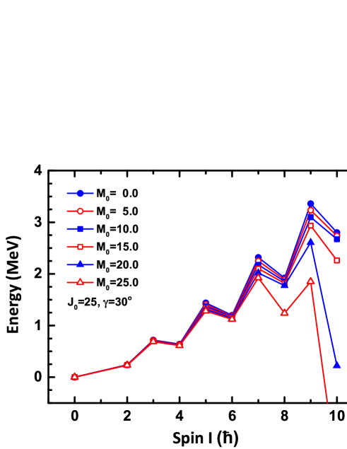
Figure 1: (Color online) Energy spectra as a function of spin $I$ calculated for the triaxial rotor model at NLO with parameters $\mathcal{J}_{0}=25~{}\hbar^{2}/\textrm{MeV}$, $\mathcal{M}_{0}=(0\dots 25)~{}\hbar^{4}/\textrm{MeV}^{3}$ and $\gamma=30^{\circ}$.

The obtained yrast energy spectra as a function of spin $I$ are shown in Fig. 1. One sees that with increasing $\mathcal{M}_{0}$, the energy eigenvalues decrease. This feature is due to the negative sign of $\Delta\mathcal{H}_{\textrm{NLO}}$. Because $\Delta\mathcal{H}_{\textrm{NLO}}$ contains the fourth power of spin, the impact of $\Delta\mathcal{H}_{\textrm{NLO}}$ for the high spin states is larger than those for the low spin states. In addition, if $\mathcal{M}_{0}$ is very large ($\mathcal{M}_{0}\geq 20~{}\hbar^{4}/\textrm{MeV}^{3}$), the corrections from $\Delta\mathcal{H}_{\textrm{NLO}}$ lead to irregular energy spectra. In this case, the power counting is not longer obeyed, and the limits of the EFT are exceeded.

III Numerical details

In the following, the newly developed EFT for the triaxial rotor is applied to describe the experimental ground state and $\gamma$ bands for the isotopes ¹⁰²Ru up to ¹¹²Ru. The data are taken from the compilation of the National Nuclear Data Center (NNDC) . In the calculations, both $\mathcal{J}_{k}$ and $\mathcal{M}_{k}$ are assumed to be of the irrotational type, see Eqs. (37) and (38). As a first strategy, $\mathcal{J}_{0}$ and $\mathcal{M}_{0}$ are fitted to the experimental energies of the lowest members of the ground state band, $0_{1}^{+}$, $2_{1}^{+}$, $4_{1}^{+}$, $6_{1}^{+}$, while the triaxial deformation parameter $\gamma$ is taken from the covariant density functional theory (CDFT) calculations employing the effective interaction PC-PK1 Zhao et al. (2010). In these constrained CDFT calculations, the Dirac equation for a nucleon is solved in a three-dimensional harmonic oscillator basis, which in the present case includes 12 major oscillator shells. The pairing correlations are treated within the BCS scheme utilizing a delta pairing-force. The obtained energy spectra will be compared with the results of the five-dimensional collective Hamiltonian (5DCH) Niks̆ić et al. (2011) in order to examine the applicability of the present EFT approach.

In the 5DCH calculations, both the collective potential and the inertial parameters are calculated with the constrained CDFT using the effective interaction PC-PK1 Zhao et al. (2010). In the calculations of the moments of inertia $\mathcal{J}_{k}$, the Inglis-Belyaev formula is used Ring and Schuck (1980). It usually underestimates the experimental moments of inertia due to the absence of the contributions from time-odd nuclear mean-fields and the absence of the so-called Thouless-Valatin (TV) dynamical rearrangement contributions Li et al. (2012). The proper inclusion of these effects requires very demanding computations. In order to account for these in an approximate way, one multiplies the moments of inertia (using the Inglis-Belyaev formula) with a fudge factor $f$, that is fitted to reproduce the energy of the experimentalvalue of the $2_{1}^{+}$ state.

As a second strategy, the three parameters $\mathcal{J}_{0}$, $\mathcal{M}_{0}$, and $\gamma$ are fitted to the data. This corresponds to a genuine EFT approach supplemented by the condition of irrotational moments of inertia, which is common for the triaxially deformed nuclei considered in this work. We do not consider the case where all the $\mathcal{J}_{k}$ and $\mathcal{M}_{k}$ are determined from a fit to the data. In that case, one would have to fit 3 (6) parameters at LO (NLO).

The results based on this approach are compared to those from the first strategy to order to examine the quality of covariant density functional theory (CDFT) in predicting triaxial deformations of nuclei.

IV Results and discussion

IV.1 Quasi-particle alignment analysis

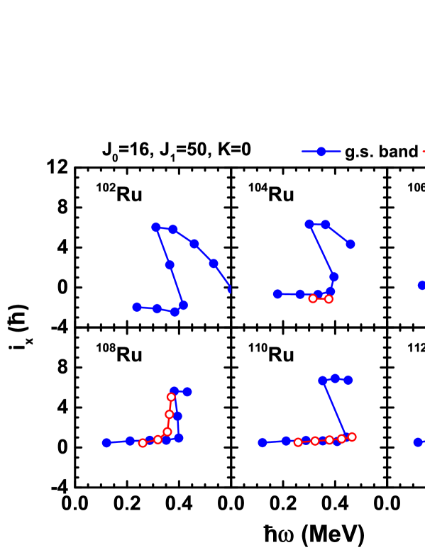
Figure 2: (Color online) Quasi-particle alignments of ground state and $\gamma$ bands for the isotopes ${}^{102\textrm{-}112}$Ru. The calculations at $K=0$ were performed with Harris parameters $\mathfrak{J}_{0}=16.0~{}\hbar^{2}/\textrm{MeV}$ and $\mathfrak{J}_{1}=50.0~{}\hbar^{2}/\textrm{MeV}^{3}$.

In order to establish the applicability of the triaxial rotor model (TRM), we study first the quasi-particle alignment of the experimental energy spectra as described in Ref. Bengtsson and Frauendorf (1979). The quasi-particle alignment $i_{x}$ is defined as the difference between the spin of the data and that of a reference rotor (with moment of inertia ${\mathfrak{J}}_{0}+\omega^{2}{\mathfrak{J}_{1}}$). Such an empirical study provides information about the spin at which a nucleon-pair breaks and thus the collective rotor model becomes inapplicable. We consider the $K=0$ band and choose for the so-called Harris parameters $\mathfrak{J}_{0}=16.0~{}\hbar^{2}/\textrm{MeV}$ and $\mathfrak{J}_{1}=50.0~{}\hbar^{2}\textrm{MeV}^{3}$, which describe the dependence of moments of inertia on the rotational frequency in the form $\mathfrak{J}_{0}+\omega^{2}\mathfrak{J}_{1}$. The obtained alignments $i_{x}$ as a function of the rotational frequency $\omega$ are shown in Fig. 2. In all cases, the calculated alignments display a nearly constant behavior at low $\hbar\omega$ (corresponding to spins $I\leq 10$) whereas a drastic increase sets in at higher $\hbar\omega$. For this reason the range of applicability of the TRM and 5DCH Hamiltionians is restricted to the region with spins $I\leq 10$. Therefore, we consider in the following only energy spectra in this low-spin region.

IV.2 ¹¹²Ru

In this subsection, the ¹¹²Ru nucleus is selected to demonstrate the applicability of the EFT in the description of collective rotations of triaxially deformed nuclei. In the TRM calculations, the triaxial deformation parameter $\gamma$ as obtained from constrained CDFT calculations is used in the first fit strategy. Fig. 3 shows contour lines of constant potential energy in the $\beta\gamma$-plane as obtained with the PC-PK1 effective interaction Zhao et al. (2010). The potential energy is measured with respect to its absolute minimum (marked by a square in Fig. 3). It is found that the ground state of ¹⁰²Ru has the deformation parameters $\beta=0.26$ and $\gamma=38.4^{\circ}$ as well as a moderate $\gamma$-softness.

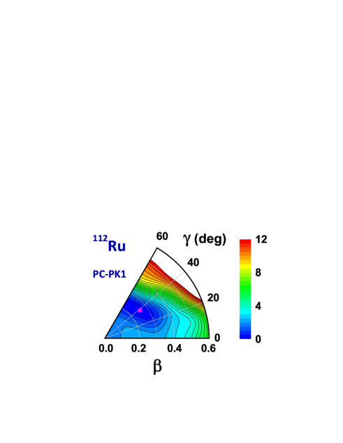
Figure 3: (Color online) Contour lines of constant potential energy in the $\beta\gamma$-plane for the ground-state configuration of ¹¹²Ru calculated in constrained covariant density functional theory with the effective interaction PC-PK1. Energies (in MeV) are measured with respect to the absolute minimum indicated by a square. The energy separation between neighboring contour lines is 0.5 MeV.

With the given triaxial deformation parameter $\gamma=38.4^{\circ}$, the other moment of inertia parameters $\mathcal{J}_{0}$ and $\mathcal{M}_{0}$ of the irrotational TRM are determined by fitting to the experimental data. In the LO calculation, the value of $\mathcal{J}_{0}$ is $\mathcal{J}_{0}=25.43~{}\hbar^{2}/\textrm{MeV}$. Fixing this value and performing the the NLO calculation gives $\mathcal{M}_{0}=1.59~{}\hbar^{4}/\textrm{MeV}^{3}$ for the non-rigidity parameter. If $\mathcal{J}_{0}$ and $\mathcal{M}_{0}$ are simultaneously fitted to the data in an NLO calculation, one obtains somewhat different values, $\mathcal{J}_{0}=24.76~{}\hbar^{2}/\textrm{MeV}$ and $\mathcal{M}_{0}=4.97~{}\hbar^{4}/\textrm{MeV}^{3}$. The corresponding energy spectra of the ground state and $\gamma$ bands are shown in Fig. 4 as a function of spin $I$ in comparison to the results of the 5DCH Hamiltonian. One observes that that both the LO and NLO calculation provide a reasonable description of the experimental data. In the LO calculation the energies of ground states $8_{1}^{+}$ and $10_{1}^{+}$ are somewhat overestimated and the description of the $\gamma$ band in high-spin region $I\geq 6$ is not as good as for low spins. In the case of NLO calculation with $\mathcal{J}_{0}$ fixed, the obtained results are very similar to those at LO, since $\mathcal{M}_{0}$ is small and thus only small corrections are involved. In the case where $\mathcal{J}_{0}$ and $\mathcal{M}_{0}$ are simultaneously fitted, the description of the data is somewhat improved. Nevertheless, there are still some deviations for the high-spin states in the $\gamma$ band. By comparing with the 5DCH calculation, which reproduces better the ground state and $\gamma$ bands, one can attribute the deviations in the TRM to the neglect of the vibrational degrees of freedom. Consequently, in the future one should include systematically the vibrational degrees of freedom in the EFT.

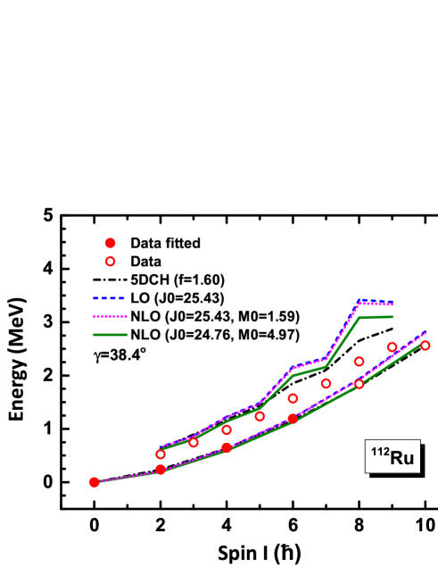
Figure 4: (Color online) Energy spectra for the ground state and $\gamma$ band in ¹¹²Ru calculated in the triaxial rotor model at LO and NLO in comparison to results of the 5-dimensional collective Hamiltonian (5DCH).

In Fig. 5, we show the results obtained by the second strategy, where $\mathcal{J}_{0}$, $\mathcal{M}_{0}$, and $\gamma$ are fitted simultaneously to the data, and compare them with those of the first strategy. The corresponding parameter values are $\mathcal{J}_{0}=24.76~{}\hbar^{2}/\textrm{MeV}$, $\mathcal{M}_{0}=7.77~{}\hbar^{4}/\textrm{MeV}^{3}$, and $\gamma=32.1^{\circ}$. Note that $\gamma$ is close to the value given by the CDFT calculation, suggesting that the triaxial deformation predicted by CDFT is quite reliable. From Fig. 5, one observes that the description of the ground state band is similar in both strategies. The same feature applies to the calculated $\gamma$ bands. It is comforting to see that the effective field theory without any external input works equally well as the (more microscopic) CDFT calculation.

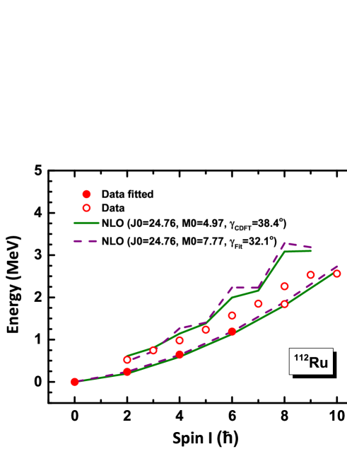
Figure 5: (Color online) Same as Fig. 4. The results of both strategies are compared with each other (see the text for details).

IV.3 Isotopes ¹⁰²Ru up to ¹¹⁰Ru

After the successful description of ¹¹²Ru, one can perform analogous calculations for the lighter isotopes ¹⁰²Ru up to ¹¹⁰Ru. Such a systematic study over a long chain of isotopes provides further tests of the applicability of the EFT.

In Fig. 6, the contour lines of constant potential energy in the $\beta\gamma$-plane are shown for ¹⁰²Ru up to ¹¹²Ru. One observes that all potential energy surfaces possess a triaxially deformed minimum and they exhibit softness along the $\gamma$-direction. The sequence of plots in Fig. 6 shows that with increasing neutron number the $\gamma$-coordinate of the minimum becomes larger. These angles $\gamma$ together with the $\beta$-coordinate at the minimum are listed in Table 1. One observes that $\gamma$ doubles from $19.2^{\circ}$ to $38.4^{\circ}$ when the mass number ranges from 102 to 112. The values in Table 1 provide the input to the EFT calculations based on the first fit strategy.

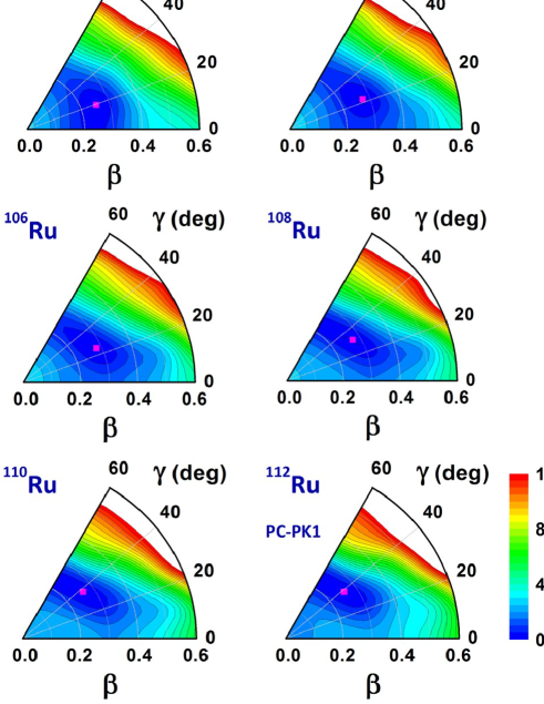
Figure 6: (Color online) Contour lines of constant potential energy in the $\beta\gamma$-plane for the ground-state configuration of the isotopes ${}^{102\textrm{-}112}$Ru.

Table 1: Deformation parameters $(\beta,\gamma)$ of the ground state in ${}^{102\textrm{-}112}$Ru calculated with the constrained CDFT employing the PC-PK1 effective interaction.

Nucleus	$(\beta,\gamma)$	Nucleus	$(\beta,\gamma)$
102Ru	$(0.25,19.2^{\circ})$	104Ru	$(0.28,22.2^{\circ})$
106Ru	$(0.28,24.9^{\circ})$	108Ru	$(0.27,31.9^{\circ})$
110Ru	$(0.26,37.6^{\circ})$	112Ru	$(0.26,38.4^{\circ})$

In Fig. 7, the energy spectra of the ground state and $\gamma$ bands in the isotopes ¹⁰²Ru up to ¹¹²Ru calculated at LO and NLO are shown in comparison to experimental data and results from the 5DCH Hamiltionian. We find similar results and draw the same conclusions for these lighter Ru isotopes as for ¹¹²Ru. Overall, the description at NLO is better than at LO, but there are still some deviations between the NLO results and the data for the high spin states in the $\gamma$ bands. Since the 5DCH results are in good agreement with the data, this points again towards the importance of including vibrational degrees of freedom in the EFT formulation.

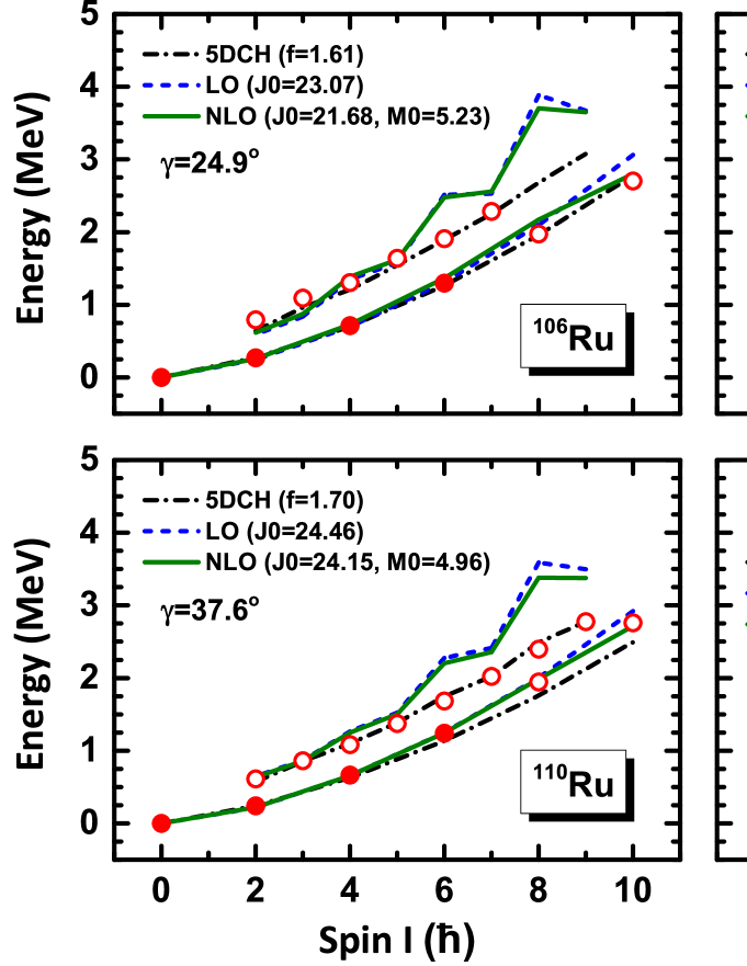
Figure 7: (Color online) Same as Fig. 4, but for ¹⁰²Ru up to ¹¹²Ru.

As we have mentioned, the inertial parameters of the 5DCH Hamiltonian are calculated with the CDFT. In Fig. 8, the three principal moments of inertia $\mathcal{J}_{1,2,3}$ of the ground state are compared to those determined at NLO over the mass region 102$-$112. One finds appreciable differences and therefore the non-rigidity parameters $\mathcal{M}_{k}$ ($k=1$, 2, 3) should also be extracted from constrained CDFT calculations in the future. This way all parameters of the triaxial rotor model (TRM) at NLO would be determined in a fully microscopic manner.

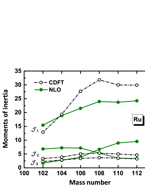
Figure 8: (Color online) Moments of inertia $\mathcal{J}_{k}$ ($k=1$, 2, 3) entering the TRM in comparison to those computed with constrained CDFT, using the triaxial deformation parameter $\gamma$ from CDFT (strategy one).

Next, we consider the results of the genuine EFT approach, where all pertinent parameters are determined from a fit to data. In Tab. 2, we give the resulting values for $\mathcal{J}_{0}$, $\mathcal{M}_{0}$ and $\gamma$ for the considered Ru isotopes considered in comparison to the values obtained in strategy one. The two sets of parameters are similar, but there some differences, most visible in the triaxial deformation parameter $\gamma$. It remains to be seen whether these differences persist if the vibrational degrees of freedom are included in the EFT formulation. The energies in the ground state and the $\gamma$ band at NLO are displayed in Fig. 9 for both fit strategies and the resulting description of all data turns out to be very similar in both approaches.

Table 2: Parameters used in the NLO calculations for strategy one (I) and two (II). The units of $\mathcal{J}_{0}$ and $\mathcal{M}_{0}$ are $\hbar^{2}/\textrm{MeV}$ and $\hbar^{4}/\textrm{MeV}^{3}$, respectively.

	Nucleus	102Ru	104Ru	106Ru	108Ru	110Ru	112Ru
	$\gamma_{\textrm{CDFT}}$	$19.2^{\circ}$	$22.2^{\circ}$	$24.9^{\circ}$	$31.9^{\circ}$	$37.6^{\circ}$	$38.4^{\circ}$
I	$\mathcal{J}_{0}$	16.00	19.25	21.68	24.02	24.15	24.76
	$\mathcal{M}_{0}$	0.80	2.47	5.23	9.02	4.96	4.97
	$\gamma_{\textrm{Fit}}$	$24.7^{\circ}$	$28.0^{\circ}$	$29.9^{\circ}$	$33.6^{\circ}$	$33.8^{\circ}$	$32.1^{\circ}$
II	$\mathcal{J}_{0}$	17.42	18.11	22.85	23.65	23.81	24.76
	$\mathcal{M}_{0}$	1.23	4.56	4.54	8.76	7.07	7.77

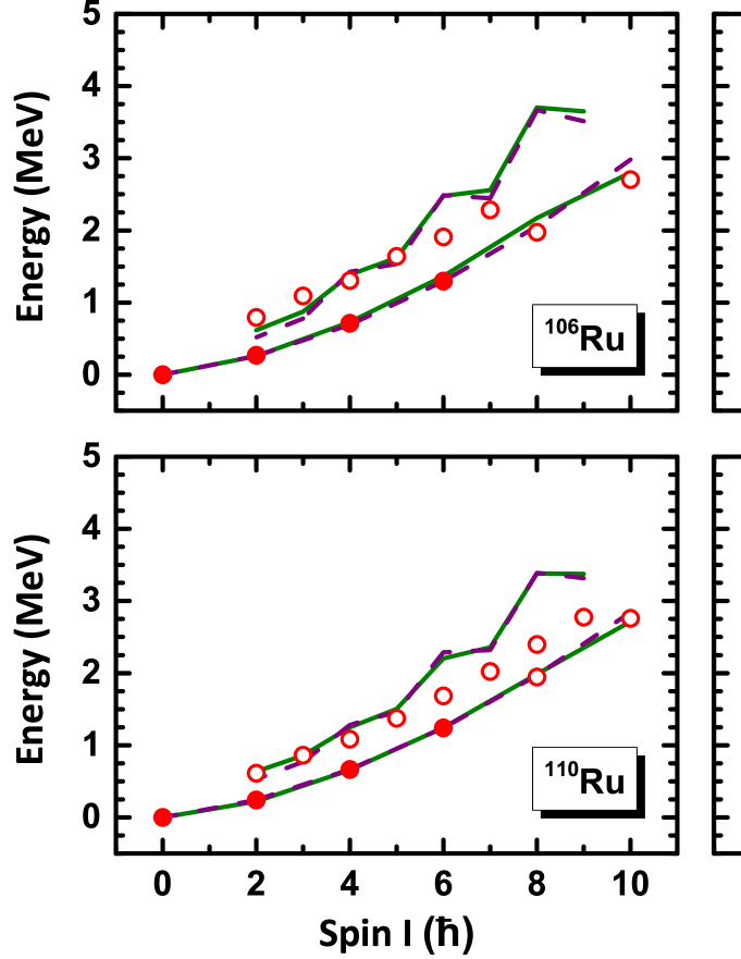
Figure 9: (Color online) Energy spectra for the ground state and $\gamma$-bands in ¹⁰²Ru up to ¹¹²Ru at NLO taking the triaxial deformation parameter $\gamma$ from the 5DCH calculation (solid green lines) or directly from the EFT fit (dashed purple lines).

V Summary

In this work the effective field theory for the collective rotational motion has been generalized to triaxially deformed nuclei. The Hamiltonian of the triaxial rotor model has been constructed up to next-to-leading order in the EFT power counting. Taking the energy spectra of the ground state and $\gamma$ bands of the even isotopes ¹⁰²Ru up to ¹⁰²Ru as benchmarks, the applicability of the EFT has been examined by describing the pertinent data for spins $I\leq 10$ and by comparing to results obtained with a five-dimensional collective Hamiltonian. It is found that the description at NLO is overall better than at LO. Nevertheless, there are still some deviations between the NLO calculation and the data for high-spin states in the $\gamma$ bands. This points towards the importance of including vibrational degrees of freedom in the EFT formulation.

In addition, we have compared two strategies of fitting parameters. In the first strategy, $\gamma$ is taken from a CDFT calculation, and in the second strategy, $\gamma$ is also fitted to the data (the genuine EFT approach). The corresponding results show that the EFT for collective nuclear rotation can be applied without referring to any microscopic (model-dependent) input. We have found that the value of $\gamma$ as obtained in the second strategy is close to the one predicted by CDFT. This suggests that CDFT is a reliable microscopic approach to calculate ground state properties. Hence, we can (but need not) combine EFT and CDFT to describe the rotational spectra of deformed nuclei.

The results presented give us a strong motivation to further generalize the EFT for triaxially deformed nuclei with odd mass number and to include systematically the vibrational degrees of freedom.

References

- Bohr and Mottelson (1975) A. Bohr and B. R. Mottelson, Nuclear structure, vol. II (Benjamin, New York, 1975).
- Iachello and Arima (1987) F. Iachello and A. Arima, The interacting boson model (Cambridge University Press, Cambridge, 1987).
- Papenbrock (2011) T. Papenbrock, Nucl. Phys. A 852, 36 (2011).
- Zhang and Papenbrock (2013) J. L. Zhang and T. Papenbrock, Phys. Rev. C 87, 034323 (2013).
- Papenbrock and Weidenmüller (2014) T. Papenbrock and H. A. Weidenmüller, Phys. Rev. C 89, 014334 (2014).
- Papenbrock and Weidenmüller (2015) T. Papenbrock and H. A. Weidenmüller, J. Phys. G: Nucl. Part. Phys. 42, 105103 (2015).
- Papenbrock and Weidenmüller (2016) T. Papenbrock and H. A. Weidenmüller, Phys. Scr. 91, 053004 (2016).
- Coello Pérez and Papenbrock (2015a) E. A. Coello Pérez and T. Papenbrock, Phys. Rev. C 92, 014323 (2015a).
- Coello Pérez and Papenbrock (2015b) E. A. Coello Pérez and T. Papenbrock, Phys. Rev. C 92, 064309 (2015b).
- Coello Pérez and Papenbrock (2016) E. A. Coello Pérez and T. Papenbrock, Phys. Rev. C 94, 054316 (2016).
- van Kolck (1994) U. van Kolck, Phys. Rev. C 49, 2932 (1994).
- Epelbaum et al. (2009) E. Epelbaum, H.-W. Hammer, and U.-G. Meißner, Rev. Mod. Phys. 81, 1773 (2009).
- Ren et al. (2016) X.-L. Ren, K.-W. Li, L.-S. Geng, B.-W. Long, P. Ring, and J. Meng, arXiv: nucl-th, 1612.08482 (2016).
- Bertulani et al. (2002) C. Bertulani, H.-W. Hammer, and U. van Kolck, Nucl. Phys. A 712, 37 (2002).
- Hammer and Phillips (2011) H.-W. Hammer and D. Phillips, Nucl. Phys. A 865, 17 (2011).
- Ryberg et al. (2014) E. Ryberg, C. Forssén, H.-W. Hammer, and L. Platter, Phys. Rev. C 89, 014325 (2014).
- Bedaque and van Kolck (2002) P. F. Bedaque and U. van Kolck, Annu. Rev. Nucl. Part. Sci. 52, 339 (2002).
- Grießhammer et al. (2012) H. Grießhammer, J. McGovern, D. Phillips, and G. Feldman, Prog. Part. Nucl. Phys. 67, 841 (2012).
- Hammer et al. (2013) H.-W. Hammer, A. Nogga, and A. Schwenk, Rev. Mod. Phys. 85, 197 (2013).
- Bengtsson et al. (1984) R. Bengtsson, H. Frisk, F. May, and J. Pinston, Nucl. Phys. A 415, 189 (1984).
- Hamamoto and Sagawa (1988) I. Hamamoto and H. Sagawa, Phys. Lett. B 201, 415 (1988).
- Frauendorf and Meng (1997) S. Frauendorf and J. Meng, Nucl. Phys. A 617, 131 (1997).
- Meng et al. (2006) J. Meng, J. Peng, S. Q. Zhang, and S.-G. Zhou, Phys. Rev. C 73, 037303 (2006).
- Coleman et al. (1969) S. Coleman, J. Wess, and B. Zumino, Phys. Rev. 177, 2239 (1969).
- Callan et al. (1969) C. G. Callan, S. Coleman, J. Wess, and B. Zumino, Phys. Rev. 177, 2247 (1969).
- Brauner (2010) T. Brauner, Symmetry 2, 609 (2010).
- Ring and Schuck (1980) P. Ring and P. Schuck, The nuclear many body problem (Springer Verlag, Berlin, 1980).
- Zhao et al. (2010) P. W. Zhao, Z. P. Li, J. M. Yao, and J. Meng, Phys. Rev. C 82, 054319 (2010).
- Niks̆ić et al. (2011) T. Niks̆ić, D. Vretenar, and P. Ring, Prog. Part. Nucl. Phys. 66, 519 (2011).
- Li et al. (2012) Z. P. Li, T. Nikšić, P. Ring, D. Vretenar, J. M. Yao, and J. Meng, Phys. Rev. C 86, 034334 (2012).
- Bengtsson and Frauendorf (1979) R. Bengtsson and S. Frauendorf, Nucl. Phys. A 327, 139 (1979).