Stable Lévy processes, self-similarity
and the unit ball^∗

Abstract.

Around the 1960s a celebrated collection of papers emerged offering a number of explicit identities for the class of isotropic Lévy stable processes in one and higher dimensions; these include, for example, the lauded works of Ray (1958); Widom (1961); Rogozin (1972) (in one dimension) and Blumenthal et al. (1961); Getoor (1966); Port (1969) (in higher dimension), see also more recently Byczkowski et al. (2009); Luks (2013). Amongst other things, these results nicely exemplify the use of standard Riesz potential theory on the unit open ball $\mathbb{B}_{d}:=\{x\in\mathbb{R}^{d}:|x|<1\}$, $\mathbb{R}^{d}\backslash\mathbb{B}_{d}$ and the sphere $\mathbb{S}_{d-1}:=\{x\in\mathbb{R}^{d}:|x|=1\}$ with the, then, modern theory of potential analysis for Markov processes.

Following initial observations of Lamperti (1972), with the occasional sporadic contributions such as Kiu (1980); Vuolle-Apiala and Graversen (1986); Graversen and Vuolle-Apiala (1986), an alternative understanding of Lévy stable processes through the theory of self-similar Markov processes has prevailed in the last decade or more. This point of view offers deeper probabilistic insights into some of the aforementioned potential analytical relations; see for example Bertoin and Yor (2002); Bertoin and Caballero (2002); Caballero and Chaumont (2006a, b); Chaumont et al. (2009); Patie (2009, 2012); Bogdan and Żak (2006); Patie (2012); Kyprianou et al. (2014); Kuznetsov et al. (2014); Kyprianou and Watson (2014); Kuznetsov and Pardo (2013); Kyprianou (2016); Kyprianou et al. (2016a, b); Alili et al. (2017).

In this review article, we will rediscover many of the aforementioned classical identities in relation to the unit ball by combining elements of these two theories, which have otherwise been largely separated by decades in the literature. We present a dialogue that appeals as much as possible to path decompositions. Most notable in this respect is the Lamperti-Kiu decomposition of self-similar Markov processes given in Kiu (1980); Chaumont et al. (2013); Alili et al. (2017) and the Riesz–Bogdan–Żak transformation given in Bogdan and Żak (2006).

Some of the results and proofs we give are known (marked $\heartsuit$), some are mixed with new results or methods, respectively, (marked $\diamondsuit$) and some are completely new (marked $\clubsuit$). We assume that the reader has a degree of familiarity with the bare basics of Lévy processes but, nonetheless, we often include reminders of standard material that can be found in e.g. Bertoin (1996), Sato (2013) or Kyprianou (2014).

Part I Stable processes, self-similar Markov processes and MAPs

In this review article, we give an extensive overhaul of some aspects of the theory of strictly stable Lévy processes as seen from the point of view of self-similarity. Our presentation takes account of a sixty-year span of literature. As we walk the reader through a number of classical and recent results, they will note that the statements of results and their proofs are marked with one of three symbols. For statements or proofs which are known, we use the mark $\heartsuit$; for those statements or proofs which are known, but mixed with new results or methods (respectively), we use the mark $\diamondsuit$; for those statements or proofs which are completely new, we use the mark $\clubsuit$.

I.1. Introduction

We can define the family of stable Lévy processes as being those $\mathbb{R}$-valued stochastic processes which lie at the intersection of the class of Lévy processes and the class of self-similar processes. Whilst the former class insists on càdlàg paths and stationary and independent increments, a process $X=(X_{t},t\geq 0)$ with probabilities $\mathbb{P}_{x}$, $x\in\mathbb{R}^{d}$, in the latter class has the property that there exists a stability index $\alpha$ such that, for $c>0$ and $x\in\mathbb{R}^{d}\setminus\{0\}$,

$$\text{under }\mathbb{P}_{x},\text{ the law of }(cX_{c^{-\alpha}t},t\geq 0)\text{ is equal to }\mathbb{P}_{cx}.$$ (1)

What we call stable Lévy processes here are known in the literature as strictly stable Lévy processes, but for the sake of brevity we will henceforth refer to them as just stable processes as there will be no confusion otherwise.

Living in the intersection of self-similar Markov processes and Lévy processes, it turns out that stable processes are useful prototypes for exemplifying the theory of both fields as well as for examining phenomena of processes with path discontinuities and how they differ significantly from e.g. the theory of diffusions; see for example Döring and Kyprianou (2018) for recent results showing discrepancies with Feller’s classical boundary classification for diffusions in one-dimension for stochastic differential equations driven by stable processes.

In a large body of the literature concerning stable processes it is usual to restrict the study of stable processes to those that are distributionally isotropic. That is to say, those processes for which, for all orthogonal transforms $B:\mathbb{R}^{d}\to\mathbb{R}^{d}$ and $x\in\mathbb{R}^{d}$,

$$\text{under }\mathbb{P}_{x},\text{ the law of }(BX_{t},t\geq 0)\text{ is equal to }\mathbb{P}_{Bx}.$$

As such, we talk about isotropic stable processes. The restriction to the isotropic subclass already presents sufficient challenges, whilst allowing for one more mathematical convenience. That said, we can and will drop the assumption of isotropy, but in dimension $d=1$ only. For dimension $d\geq 2$, we will always work in the isotropic setting. It remains to be seen how rich the development of the literature on stable processes will become in the future without the assumption of isotropy in higher dimensions.

It turns out that stable processes necessarily have index of stability $\alpha$ which lies in the range $(0,2]$. The case $\alpha=2$, in any dimension, pertains to Brownian motion and therefore necessarily has continuous paths. Somewhat dogmatically we will exclude this parameter choice from our discussion for the simple reason that we want to explore phenomena which can only occur as a consequence of jumps. That said, we pay occasional lip service to the Brownian setting.

Henceforth, $X:=(X_{t}:t\geq 0)$, with probabilities $\mathbb{P}_{x}$, $x\in\mathbb{R}^{d}$, will denote a $d$-dimensional isotropic stable process with index of similarity $\alpha\in(0,2)$. For convenience, we will always write $\mathbb{P}$ in place of $\mathbb{P}_{0}$.

I.1.1. One-dimensional stable processes

When $d=1$, as alluded to above, we will be more adventurous and permit anistropy. It is therefore inevitable that a second parameter is needed which will code the degree of asymmetry. To this end, we introduce the positivity parameter $\rho:=\mathbb{P}(X_{1}\geq 0)$. This parameter as well as $\hat{\rho}:=1-\rho$ will appear in most identities. A good case in point in this respect is the Lévy measure of $X$ and another is its characteristic exponent. The former is written

$$\Pi({\textnormal{d}}x):=\frac{\Gamma(\alpha+1)}{\pi}\left\{\frac{\sin(\pi\alpha\rho)}{x^{\alpha+1}}\mathbf{1}_{(x>0)}+\frac{\sin(\pi\alpha\hat{\rho})}{{|x|}^{\alpha+1}}\mathbf{1}_{(x<0)}\right\}{\textnormal{d}}x,\qquad x\in\mathbb{R},$$ (2)

and the latter takes the form

$$\Psi(\theta) :=-\frac{1}{t}\log\mathbb{E}[{\rm e}^{{{\rm i}\theta X_{t}}}]$$

$$=|\theta|^{\alpha}({\rm e}^{\pi{\textnormal{i}}\alpha(\frac{1}{2}-\rho)}\mathbf{1}_{(\theta>0)}+{\rm e}^{-\pi{\textnormal{i}}\alpha(\frac{1}{2}-\rho)}\mathbf{1}_{(\theta<0)}),\qquad\theta\in\mathbb{R},t>0.$$ (3)

For a derivation of this exponent, see Exercise 1.4 of Kyprianou (2014) or Chapter 3 of Sato (2013).

It is well known that the transition semigroup of $X$ has a density with respect to Lebesgue measure. That is to say,

$${\texttt{p}}_{t}(x):=\frac{1}{2\pi}\int_{\mathbb{R}}{\rm e}^{-{\textnormal{i}}zx}{\rm e}^{-\Psi(z)t}{\textnormal{d}}z,\qquad x\in\mathbb{R},t>0,$$ (4)

exists and satisfies

$$\mathbb{P}_{x}(X_{t}\in{\textnormal{d}}y)=\texttt{p}_{t}(y-x){\textnormal{d}}y$$ (5)

for all $x,y\in\mathbb{R}$ and $t>0$.

In one dimension, we are predominantly interested in the fluctuations of $X$ when it moves both in an upward and a downward direction. The aforesaid exclusion can be enforced by requiring throughout that

both $\alpha\rho$ and $\alpha\hat{\rho}$ belong to $(0,1)$.

This excludes both the case stable subordinators, the negative of stable subordinators (when $\rho=1$ or $\hat{\rho}=1$, respectively) and spectrally negative and positive processes (when $\alpha\rho=1$ or $\alpha\hat{\rho}=1$, respectively).

Stable processes are one of the few known classes of Lévy processes which reveal a significant portion of the general theory in explicit detail. We will spend a little time here recalling some of these facts.

As one dimensional Lévy processes with two-sided jumps, we can talk about their running maximum process $\overline{X}_{t}:=\sup_{s\leq t}X_{s}$, $t\geq 0$, and their running minimum process $\underline{X}_{t}:=\inf_{s\leq t}X_{s}$. As is the case with all Lévy processes, it turns out that the range of $\overline{X}$ agrees with that of a subordinator, say $H$, called the ascending ladder height processes. By subordinator we mean a Lévy process with increasing paths and we allow the possibility that it is killed at a constant rate and sent to a cemetery state, taken to be $+\infty$. The inclusion of a killing rate depends on whether the underlying Lévy process drifts to $-\infty$ (resp. $+\infty$), in which case $\overline{X}_{\infty}<\infty$ (resp. $-\underline{X}_{\infty}<\infty$) almost surely or oscillates (in which case $\overline{X}_{\infty}=-\underline{X}_{\infty}=\infty$). When the process drifts to $-\infty$, the killing rate is strictly positive, otherwise it is zero (i.e. no killing).

Roughly speaking the subordinator $H$ can be thought of as the trajectory that would remain if we removed the sections of path, or better said, if we removed the excursions of $X$, which lie between successive increments of $\overline{X}$ and the temporal gaps created by this removal procedure are closed. Similarly the range of $-\underline{X}$ agrees with that of a subordinator, say $\hat{H}$, called the descending ladder height process. Naturally the two processes $H$ and $\hat{H}$ are corollated. For more background on the ladder height processes see Chapter VI of Bertoin (1996) or Chapter 6 of Kyprianou (2014).

Suppose that we denote the Laplace exponent of $H$ by $\kappa$. To be precise,

$$\kappa(\lambda)=\frac{1}{t}\log\mathbb{E}[{\rm e}^{-\lambda H_{t}}],\qquad t,\lambda\geq 0,$$

where, necessarily, the exponent $\kappa$ is a Bernstein function with general form

$$\kappa(\lambda)=q+\delta\lambda+\int_{(0,\infty)}(1-{\rm e}^{-\lambda x})\Upsilon({\rm d}x),\qquad\lambda\geq 0,$$ (6)

Here, $q\geq 0$ is the killing rate, $\delta\geq 0$ is a linear drift and $\Upsilon$ is the Lévy measure of $H$. (See Schilling et al. (2012) for more on Bernstein functions in the context of subordinators.) The Laplace exponent of $\hat{H}$, which we shall henceforth denote by $\hat{\kappa}$, is similarly described. Note that the Laplace exponent of both the ascending and descending ladder height processes can be extended analytically to $\{z\in\mathbb{C}:{\rm{Re}}(z)\geq 0\}$.

It is a remarkable fact that the characteristic exponent of every Lévy process factorises into two terms, each one exposing the Laplace exponent of the ascending and descending ladder height processes respectively. That is to say, up to a multiplicative constant, we have

$$\Psi({z})=\kappa(-{\rm i}{z})\hat{\kappa}({\rm i}{z}),\qquad{z}\in\mathbb{R}.$$ (7)

This equality is what is commonly referred to as the Wiener–Hopf factorization; see Chapter VI of Bertoin (1996) or Chapter 6 of Kyprianou (2014).

In the stable case, for $\theta\geq 0$,

$$\kappa(\theta)=\theta^{\alpha\rho}\text{ and }\hat{\kappa}(\theta)=\theta^{\alpha\hat{\rho}}.$$

Notably, $H$ is a stable subordinator with no killing and no drift (and hence, by exchanging the roles of $\rho$ and $\hat{\rho}$, the same is true of $\hat{H}$). It is a pure jump subordinator with Lévy intensity

$$\Upsilon({\textnormal{d}}x)=\frac{\alpha\rho}{\Gamma(1-\alpha\rho)}\frac{1}{x^{1+\alpha\rho}}{\textnormal{d}}x,\qquad x>0$$ (8)

(again, with the same being true for $\hat{H}$, albeit with the roles of $\rho$ and $\hat{\rho}$ reversed). An explicit understanding of the Wiener–Hopf factorisation is important from the perspective of understanding how one-dimensional stable process cross levels for the first time, the precursor of the problem we will consider here in higher dimensions. Indeed, consider the first passage time $\tau^{+}_{a}=\inf\{t>0:X_{t}>a\}$, for $a>0$;

$$\text{the overshoot of $X$ above $a$ is defined as $X_{\tau^{+}_{a}}-a$}.$$

As the reader may already guess, the scaling property of stable processes suggests that, to characterise overshoots above all levels $a$, it is sufficient to characterise overshoots above level 1. Indeed, for each constant $c>0$, suppose we define ${X}^{c}_{t}=cX_{c^{-\alpha}t}$, $t\geq 0$. Then

$$\tau^{+}_{a} =\inf\{t\geq 0:X_{t}>a\}$$

$$=\inf\{a^{\alpha}s>0:a^{-1}X_{a^{\alpha}s}>1\}$$

$$=a^{\alpha}\inf\{s>0:X^{1/a}_{s}>1\}.$$

Accordingly, we see that $(X_{\tau^{+}_{a}}-a)/a$ is equal in distribution to $X_{\tau^{+}_{1}}-1$.

It should also be clear that the overshoot of $(X,\mathbb{P})$ above level 1 agrees precisely with the overshoot of $(H,\mathbb{P})$ above the same level. As alluded to above, the simple and explicit form of the ascending ladder processes offers quite a rare opportunity to write down the overshoot distribution of $X$ above $1$.

A classical computation using the compensation formula for the Poisson point process of jumps tells us that for a bounded measurable function $f$ and $a\geq 0$,

$$\mathbb{E}[f(H_{\tau^{+}_{1}}-1)] =\mathbb{E}\left[\sum_{t>0}f(H_{t}-1)\mathbf{1}_{(H_{t-}<1)}\mathbf{1}_{(H_{t-}+\Delta H_{t}>1)}\right]$$

$$=\mathbb{E}\left[\int_{0}^{\infty}\int_{(0,\infty)}f(H_{t}+z-1)\mathbf{1}_{(H_{t}<1)}\mathbf{1}_{(H_{t}+z>1)}\Upsilon({\textnormal{d}}z){\textnormal{d}}t\right]$$

$$=\int_{[0,1)}U({\textnormal{d}}y)\int_{(1-y,\infty)}\Upsilon({\textnormal{d}}z)f(y+z-1),$$ (9)

where $U({\textnormal{d}}x)=\int_{0}^{\infty}\mathbb{P}(H_{t}\in{\textnormal{d}}x){\textnormal{d}}t$, $x\geq 0$, is the potential of $H$. The identity in (9) was first proved in Kesten (1969a, b), see also Horowitz (1972). Noting by Fubini’s Theorem that

$$\int_{[0,\infty)}{\rm e}^{-\beta x}U({\textnormal{d}}x)=\int_{0}^{\infty}\mathbb{E}[{\rm e}^{-\beta H_{t}}]{\textnormal{d}}t=\frac{1}{\beta^{\alpha\rho}},\qquad\beta\geq 0,$$

we easily invert to find that

$$U({\textnormal{d}}x)=\Gamma(\alpha\rho)^{-1}x^{\alpha\rho-1}{\textnormal{d}}x,\qquad x>0.$$ (10)

Together with (8), we can evaluate the distribution of the overshoot over level 1 in (9). The scaling property of overshoots now gives us the following result, which is originally due to Dynkin (1961) and Lamperti (1962) and which one may refer to in potential analytic terms as the Poisson kernel on the half-line.

Lemma I.1.1 ($\heartsuit$).

For all $u,a>0$,

$$\mathbb{P}(X_{\tau^{+}_{a}}-a\in{\textnormal{d}}u)=\frac{\sin(\pi\alpha)}{\pi}\left(\frac{u}{a}\right)^{-\alpha}\left(\frac{1}{a+u}\right){\textnormal{d}}u.$$

It is not difficult to compute the total mass on $(0,\infty)$ of the distribution above using the beta integral to find that it is equal to unity. Accordingly, the probability that $X$ creeps over the level $a$ is zero, that is $\mathbb{P}(X_{\tau^{+}_{a}}=a)=0$.

We are also interested in the potential of the one-dimensional stable process. That is to say, we are interested in the potential measure

$$U(x,{\textnormal{d}}y)=\int_{0}^{\infty}\mathbb{P}_{x}(X_{t}\in{\textnormal{d}}y){\textnormal{d}}t=\left(\int_{0}^{\infty}\texttt{p}_{t}(y-x){\textnormal{d}}t\right){\textnormal{d}}y,\qquad x,y\in\mathbb{R}.$$ (11)

In order to discuss the potential, we first need to recall various notions from the theory of Lévy processes, looking in particular at the properties of transience and recurrence as well as point-recurrence.

Thanks to Kolmogorov’s zero-one law for events in the tail sigma algebra of the natural filtration $\sigma(X_{s},s\leq t)$, $t\geq 0$, for each fixed $a>0$, the convergence of the integral $\int_{0}^{\infty}\mathbf{1}_{\left(|X_{t}|<a\right)}{{\textnormal{d}}}t$ occurs with probability zero or one. Moreover, thanks to the scaling property of stable processes, if $\int_{0}^{\infty}\mathbf{1}_{\left(|X_{t}|<a\right)}{{\textnormal{d}}}t<\infty$ almost surely for some $a>0$ then this integral is almost surely convergent for all $a>0$. In that case we say that $X$ is called transient. A similar statement holds if the integral is divergent for some, and then all, $a>0$, in which case we say that $X$ is recurrent. The point of issue of $X$ is not important here thanks to spatial homogeneity.

It turns out that, more generally, this is the case for all Lévy processes. This is captured by the following classic analytic dichotomy; see for example Kingman (1964); Port and Stone (1971).

Theorem I.1.2 ($\heartsuit$).

For a Lévy process with characteristic exponent $\Psi$, it is transient if and only if, for some sufficiently small $\varepsilon>0$,

$$\int_{|{z}|<\varepsilon}{\rm{Re}}\left(\frac{1}{\Psi({z})}\right){{\textnormal{d}}}{z}<\infty,$$ (12)

and otherwise it is recurrent.

Probabilistic reasoning also leads to the following interpretation of the dichotomy.

Theorem I.1.3 ($\heartsuit$).

Let $Y$ be any Lévy process.

1. We have transience if and only if

   $$\lim_{t\to\infty}|Y_{t}|=\infty$$

   almost surely.

2. If $Y$ is not a compound Poisson process, then we have recurrence if and only if, for all $x\in\mathbb{R},$

   $$\liminf_{t\to\infty}|Y_{t}-x|=0$$ (13)

   almost surely.

Back to the stable setting, on account of the fact that

$$\int_{(-\varepsilon,\varepsilon)}{\rm{Re}}\left(\frac{1}{\Psi({z})}\right){\textnormal{d}}{z}\propto\int_{(-\varepsilon,\varepsilon)}\frac{1}{|{z}|^{\alpha}}{\textnormal{d}}{z},$$

it follows from Theorem I.1.2 that $X$ is transient whenever $\alpha\in(0,1)$ and recurrent when $\alpha\in[1,2)$. It is worth remarking here that a Lévy process which is recurrent cannot drift to $\infty$ or $-\infty$, and therefore must oscillate and we see this consistently with stable processes. On the other hand, an oscillating process is not necessarily recurrent. A nice example of this phenomenon is provided by the case of a symmetric stable process of index $0<\alpha<1$.

Returning to the issue of (11), it is clear that the potential makes no sense for $\alpha\in[1,2)$. That is to say, for each $x\in\mathbb{R}$, $U(x,A)$ assigns infinite mass to each non-empty open set $A$. When $\alpha\in(0,1)$, a general result for Lévy processes tells us that transience is equivalent to the existence of (11) as a finite measure. In the stable case, we can verify this directly thanks to the following result.

Theorem I.1.4 ($\heartsuit$).

Suppose that $\alpha\in(0,1)$. The potential of $X$ is absolutely continuous with respect to Lebesgue measure. Moreover, $U(x,{\textnormal{d}}y)=u(y-x){\textnormal{d}}y$, $x,y\in\mathbb{R}^{d}$, where

$$u(x)=\Gamma(1-\alpha)\left(\frac{\sin(\pi\alpha\rho)}{\pi}\mathbf{1}_{(x>0)}+\frac{\sin(\pi\alpha\hat{\rho})}{\pi}\mathbf{1}_{(x<0)}\right)|x|^{\alpha-1},\qquad x\in\mathbb{R}.$$ (14)

Proof ($\heartsuit$).

The proof we give here is classical. Let us first examine the expression for $u$ on the positive half-line. For positive, bounded measurable $f:[0,\infty)\to[0,\infty)$, which satisfies

$$\int_{\mathbb{R}}f(x)|x|^{\alpha-1}{\textnormal{d}}x<\infty,$$

we have

$$\int_{0}^{\infty}f(x)U(0,{\textnormal{d}}x) =\int_{0}^{\infty}\int_{0}^{\infty}f(x)\mathbb{P}(X_{t}\in{\textnormal{d}}x){\textnormal{d}}t$$

$$=\frac{1}{2\pi}\int_{0}^{\infty}f(x)\int_{\mathbb{R}}\int_{0}^{\infty}{\rm e}^{-|z|^{\alpha}t-{\textnormal{i}}zx}{\textnormal{d}}t\,{\textnormal{d}}z\,{\textnormal{d}}x$$

$$=\frac{1}{2\pi}\int_{0}^{\infty}f(x)\int_{\mathbb{R}}|z|^{-\alpha}{\rm e}^{-{\textnormal{i}}zx}\,{\textnormal{d}}z\,{\textnormal{d}}x$$

$$=\frac{{\rm e}^{-\pi{\textnormal{i}}\alpha(\frac{1}{2}-\rho)}}{2\pi}\int_{0}^{\infty}f(x)x^{\alpha-1}\int_{0}^{\infty}y^{-\alpha}{\rm e}^{-{\textnormal{i}}y}{\textnormal{d}}y\,{\textnormal{d}}x$$

$$\hskip 14.22636pt-\frac{{\rm e}^{\pi{\textnormal{i}}\alpha(\frac{1}{2}-\rho)}}{2\pi}\int_{0}^{\infty}f(x)x^{\alpha-1}\int_{0}^{\infty}y^{-\alpha}{\rm e}^{{\textnormal{i}}y}{\textnormal{d}}y\,{\textnormal{d}}x.$$ (15)

Using that the Mellin transform of ${\rm e}^{\pm{\textnormal{i}}y}$, $y\geq 0$, at $1-\alpha$ is known to be equal to $\Gamma(1-\alpha){\rm e}^{\pm{\textnormal{i}}\pi(1-\alpha)/2}$,

$$\int_{0}^{\infty}f(x)U(0,{\textnormal{d}}x) =\Gamma(1-\alpha)\frac{{\rm e}^{-\pi{\textnormal{i}}(\frac{1}{2}-\alpha\rho)}}{2\pi}\int_{0}^{\infty}f(x)x^{\alpha-1}\,{\textnormal{d}}x$$

$$\hskip 14.22636pt-\Gamma(1-\alpha)\frac{{\rm e}^{\pi{\textnormal{i}}(\frac{1}{2}-\alpha\rho)}}{2\pi}\int_{0}^{\infty}f(x)x^{\alpha-1}\,{\textnormal{d}}x$$

$$=\Gamma(1-\alpha)\frac{\sin(\pi\alpha\rho)}{\pi}\int_{0}^{\infty}f(x)x^{\alpha-1}\,{\textnormal{d}}x,$$

as required. A similar proof when $x<0$ gives the second term in (14). ∎

Write $Y$ for a general Lévy process with law ${\rm P}$, when issued from the origin. Transience and recurrence in the sense of the ${\rm P}$-almost sure convergence or divergence of $\int_{0}^{\infty}\mathbf{1}_{\left(|Y_{t}|<a\right)}{{\textnormal{d}}}t$ is a notion that pertains to the time spent visiting (open) sets. A finer notion of transience and recurrence can be developed in relation to visiting individual points.

We say that a general Lévy process can hit a point $x\in\mathbb{R}$ if

$$\mathrm{P}(Y_{t}=x\text{ for at least one }t>0)>0.$$

This notion is of course well defined for all Lévy processes. In the case of a stable process, the scaling property means that hitting a point $x$ with positive probability is equivalent to hitting any other point with positive probability. It turns out that this is generally the case for all Lévy processes, with the exception of compound Poisson processes, which may be troublesome in this respect if their jump distribution has lattice support. The following theorem, taken from Kesten (1969c), applies for the general class of Lévy processes; see also Bretagnolle (1971).

Theorem I.1.5 ($\heartsuit$).

Suppose that a general Lévy process is not a compound Poisson process and has characteristic exponent $\Psi$. Then it can hit points if and only if

$$\int_{\mathbb{R}}{\rm{Re}}\left(\frac{1}{1+\Psi({z})}\right){\textnormal{d}}z<\infty.$$ (16)

A straightforward comparison of ${\rm{Re}}\left(({1+\Psi({z})})^{-1}\right)$ with $\mathbf{1}_{(|x|<1)}+\mathbf{1}_{(|x|\geq 1)}|{z}|^{-\alpha}$ shows that (16) holds if and only if $\alpha\in(1,2)$. Therefore, referring to Theorem I.1.5, the process $X$ can hit points almost surely if and only if $\alpha\in(1,2)$. Coupled with recurrence, it is thus clear that, when $\alpha\in(1,2)$, $\mathbb{P}(X_{t}=x\text{ for at least one }t>0)=1$ for all $x\in\mathbb{R}$, showing point-recurrence. This leaves the case of $\alpha=1$ which is recurrent but not point-recurrent.

I.1.2. Higher dimensional stable processes

Recall that in dimension $d\geq 2$, we insist that $X$ is isotropic. This carries the consequence that $X$ is a $\mathbb{R}^{d}$-valued Lévy process with jump measure satisfying

$$\Pi(B) =\frac{2^{\alpha}\Gamma(({d+\alpha})/{2})}{\pi^{d/2}|\Gamma(-{\alpha}/{2})|}\int_{B}\frac{1}{|y|^{\alpha+d}}{\rm d}y$$

$$=2^{\alpha-1}\pi^{-d}\frac{\Gamma((d+\alpha)/2)\Gamma(d/2)}{\big{|}\Gamma(-\alpha/2)\big{|}}\int_{\mathbb{S}_{d-1}}r^{d-1}\sigma_{1}({\rm d}\theta)\int_{0}^{\infty}\mathbf{1}_{B}(r\theta)\frac{1}{r^{\alpha+d}}{\textnormal{d}}r,$$ (17)

for $B\in\mathcal{B}(\mathbb{R})$, where $\sigma_{1}({\textnormal{d}}\theta)$ is the surface measure on $\mathbb{S}_{d-1}$ normalised to have unit mass and the change in the constant in the second equality comes from the Jacobian when changing from Cartesian to generalised polar coordinates (see Blumenson (1960)). Equivalently, this means $X$ is a $d$-dimensional Lévy process with characteristic exponent $\Psi(\theta)=-\log\mathbb{E}({\rm e}^{{\rm i}\langle\theta,X_{1}\rangle})$ which satisfies

$$\Psi(\theta)=|\theta|^{\alpha},\qquad\theta\in\mathbb{R}^{d}.$$

Stable processes in dimension $d\geq 2$ are transient in the sense that

$$\lim_{t\to\infty}|X_{t}|=\infty$$

almost surely, from any point of issue.

Just as in the one-dimensional case, a quantity that will be of specific interest is the potential $U(x,{\textnormal{d}}y)$, which is defined just as in (11) albeit that, now, $x,y\in\mathbb{R}^{d}$. The following is classical, found, for example, in Blumenthal et al. (1961) if not earlier; see also the discussion in Example 3.4 of Bliedtner and Hansen (1986) or Section 1.1 of Landkof (1972).

Theorem I.1.6 ($\heartsuit$).

For dimension $d\geq 2$, the potential of $X$ is absolutely continuous with respect to Lebesgue measure, in which case, remembering spatial homogeneity, its density satisfies $U(x,{\textnormal{d}}y)=u(y-x){\textnormal{d}}y$, $x,y\in\mathbb{R}^{d}$, where

$$u(z)=2^{-\alpha}\pi^{-d/2}\frac{\Gamma((d-\alpha)/2)}{\Gamma(\alpha/2)}|z|^{\alpha-d},\qquad z\in\mathbb{R}^{d}.$$

Remark I.1.7.

Combining the above theorem with Theorem I.1.4, for $\rho=1/2$, one can in fact state Theorem I.1.6 more generally with the qualification that $d>\alpha$. The reader will also note that the proof given for Theorem I.1.6 below works equally well when $d=1$, $\alpha\in(0,1)$ and $\rho=1/2$.

Proof of Theorem I.1.6 ($\heartsuit$).

The proof we give here is also classical and taken from p187 of Bliedtner and Hansen (1986). Fix $\alpha\in(0,2)$ and suppose that $(S_{t},t\geq 0)$ is a stable subordinator with index $\alpha/2$. If we write $(B_{t},t\geq 0)$ for a standard $d$-dimensional Brownian motion, then it is known that $X_{t}:=\sqrt{2}B_{S_{t}}$, $t\geq 0$,is a stable process with index $\alpha$. Indeed, its stationary and independent increments and scaling, in the sense of (1), are inherited directly from those of $S$ and $B$, and are easy to verify. Note, moreover, that

$$\mathbb{E}[{\rm e}^{{\rm i}\langle\theta,X_{t}\rangle}]=\mathbb{E}\left[{\rm e}^{-|\theta|^{2}S_{t}}\right]={\rm e}^{-|\theta|^{\alpha}t},\qquad\theta\in\mathbb{R}^{d}.$$

Now note that, for bounded and measurable $f:\mathbb{R}^{d}\to[0,\infty)$, which satisfies $\int_{\mathbb{R}^{d}}f(x)|x|^{\alpha-1}{\textnormal{d}}x<\infty$,

$$\mathbb{E}\left[\int_{0}^{\infty}f(X_{t}){\textnormal{d}}t\right] =\mathbb{E}\left[\int_{0}^{\infty}f(B_{S_{t}}){\textnormal{d}}t\right]$$

$$=\int_{0}^{\infty}{\textnormal{d}}s\int_{0}^{\infty}{\textnormal{d}}t\,\mathbb{P}(S_{t}\in{\textnormal{d}}s)\int_{\mathbb{R}}\mathbb{P}(B_{s}\in{\textnormal{d}}x)f(\sqrt{2}x)$$

$$=\frac{1}{\Gamma(\alpha/2)\pi^{d/2}2^{d}}\int_{\mathbb{R}}{\textnormal{d}}y\int_{0}^{\infty}{\textnormal{d}}s\,{\rm e}^{-|y|^{2}/4s}s^{-1+(\alpha-d)/2}f(y)$$

$$=\frac{1}{2^{\alpha}\Gamma(\alpha/2)\pi^{d/2}}\int_{\mathbb{R}}{\textnormal{d}}y\,|y|^{(\alpha-d)}\int_{0}^{\infty}{\textnormal{d}}u\,e^{-u}u^{-1+(d-\alpha/2)}f(y)$$

$$=\frac{\Gamma((d-\alpha)/2)}{2^{\alpha}\Gamma(\alpha/2)\pi^{d/2}}\int_{\mathbb{R}}{\textnormal{d}}y\,|y|^{(\alpha-d)}f(y),$$

where we have used the expression for the potential of $S$ as in (10) (albeit replacing the index $\alpha\rho$ there by $\alpha$). This completes the proof. ∎

The final thing to mention in this section is the issue of hitting points for stable processes in dimension $d\geq 2$. It is known that if the condition (16) fails, then points cannot be hit from Lebesgue-almost every point of issue. Note in higher dimensions that the effect of the Jacobian comes into play when we estimate the integral in (16). Indeed, one can easily make the comparison with the integral

$$\int_{|x|>1}\frac{1}{|z|^{\alpha}}{\textnormal{d}}z\asymp\int_{1}^{\infty}\int_{\mathbb{S}_{d-1}}\frac{1}{r^{\alpha}}r^{d-1}\sigma_{1}(\theta){\textnormal{d}}z\asymp\int_{1}^{\infty}r^{d-\alpha-1}{\textnormal{d}}r=\infty,$$

as $d\geq 2$. Here, $a\asymp b$ means that $a/b$ is bounded form above and below by a strictly positive constant. Hence, for stable process, points cannot be hit from Lebesgue-almost every point of issue. However, with a little work one can upgrade this to the statement that points cannot be hit from any point of issue. The subtleties of this can be found for, example, in Chapter 8, Section 43 of Sato (2013).

I.2. Positive self-similar Markov processes and stable processes

In this section we introduce one of the key mathematical tools that we shall use to analyse stable processes: positive self-similar Markov processes. We shall often denote this class by pssMp for convenience. Shortly we will give the definition of these processes and their pathwise characterisation as space-time-changed Lévy processes through the Lamperti transform. Thereafter, we spend the rest of the section exploring a number of examples of pssMp which can be constructed through path transformations of stable processes. Each of these examples of pssMp turn out to be intimately connected, through the Lamperti transform, to a different Lévy process belonging to the (extended) hypergeometric class.

I.2.1. The Lamperti transform

Let us begin with a definition of the fundamental class of processes that will dominate our analysis.

Definition I.2.1.

A $[0,\infty)$-valued Feller process $Z=(Z_{t},t\geq 0)$ is called a positive self-similar Markov process if there exists a constant $\alpha>0$ such that, for any ${x}>0$ and $c>0$,

the law of $$(cZ_{c^{-\alpha}t},t\geq 0) {P}_{x} {P}_{c{x}}$$ under is , (18)

where ${P}_{x}$ is the law of $Z$ when issued from ${x}$. In that case, we refer to $\alpha$ as the index of self-similarity. (The reader should note that some authors prefer to refer to $1/\alpha$ as the index of self-similarity.)

In his landmark paper, Lamperti (1972) showed that there is a natural bijection between the class of exponentially killed Lévy processes and positive self-similar Markov processes, up to a naturally defined lifetime,

$$\zeta=\inf\{t>0:Z_{t}=0\},$$

the first moment $X$ visits the origin. Roughly speaking, this bijection shows that the property of self-similarity is interchangeable with the property of having stationary and independent increments through an appropriate space-time transformation. Below, we state this bijection as a theorem.

Let us first introduce some more notation. Throughout this section, we shall use $\Xi:=(\Xi_{t},t\geq 0)$ to denote a one-dimensional Lévy process (not necessarily issued from the origin) which is killed and sent to the cemetery state $-\infty$ at an independent and exponentially distributed random time, $\mathbf{e}=\inf\{t>0:\Xi_{t}=-\infty\}$, with rate in $[0,\infty)$. As usual, we understand $\mathbf{e}$ in the broader sense of an exponential distribution, so that if its rate is $0$, then $\mathbf{e}=\infty$ with probability one, in which case there is no killing.

We will be interested in applying a time change to the process $\Xi$ by using its integrated exponential process, $I:=\{I_{t}:t\geq 0\}$, where

$$I_{t}=\int_{0}^{t}{\rm e}^{\alpha\Xi_{s}}{\rm d}s,\qquad t\geq 0.$$ (19)

As the process $I$ is increasing, we may define its limit, $I_{\infty}:=\lim_{t\uparrow\infty}I_{t}$, whenever it exists. We are also interested in the inverse process of $I$:

$$\varphi(t)=\inf\{s>0:I_{s}>t\},\qquad t\geq 0.$$ (20)

As usual, we work with the convention $\inf\emptyset=\infty$.

The following theorem introduces the celebrated Lamperti transformation, which characterises all positive self-similar Markov processes. It was originally proved in Lamperti (1972); see also Chapter 13 of Kyprianou (2014). We omit the proof here as it is long and a distraction from our main objectives.

Theorem I.2.2 (The Lamperti transform $\heartsuit$).

Fix $\alpha>0$.

• If $(Z,P_{x})$, $x>0$, is a positive self-similar Markov process with index of self-similarity $\alpha$, then up to absorption at the origin, it can be represented as follows:

  $$Z_{t}\mathbf{1}_{(t<\zeta)}=\exp\{\Xi_{\varphi(t)}\},\,\qquad t\geq 0,$$ (21)

  such that $\Xi_{0}=\log x$ and either

  • $P_{x}(\zeta=\infty)=1$ for all ${x}>0$, in which case, $\Xi$ is a Lévy process satisfying $\limsup_{t\uparrow\infty}\Xi_{t}=\infty$,

  • $P_{x}(\zeta<\infty\text{ and }Z_{\zeta-}=0)=1$ for all ${x}>0$, in which case $\Xi$ is a Lévy process satisfying $\lim_{t\uparrow\infty}\Xi_{t}=-\infty$, or

  • $P_{x}(\zeta<\infty\text{ and }Z_{\zeta-}>0)=1$ for all ${x}>0$, in which case $\Xi$ is a Lévy process killed at an independent and exponentially distributed random time.

  In all cases, we may identify $\zeta=I_{\infty}$.

• Conversely, for each $x>0$, suppose that $\Xi$ is a given (killed) Lévy process, issued from $\log x$. Define

  $$Z_{t}=\exp\{\Xi_{\varphi(t)}\}\mathbf{1}_{(t<I_{\infty})},\qquad t\geq 0.$$

  Then $Z$ defines a positive self-similar Markov process up to its absorption time $\zeta=I_{\infty}$, which satisfies $Z_{0}=x$ and has index $\alpha$.

It is tempting to immediately think of a stable process as an example of a positive self-similar Markov process, but, with the exception of a stable subordinator (which has been ruled out of this discussion), it fails against the criteria of positivity. In fact, the case of a stable subordinator is precisely the example (and the only example) of a self-similar Markov processes which was given in Lamperti (1972). It is possible, however, to construct examples of positive self-similar Markov processes from path transformations of stable processes.

In all of the examples that follow to the end of this section, we will take $X$, with probabilities $\mathbb{P}_{x}$, $x\in\mathbb{R}$, to be a stable process with two-sided jumps.

I.2.2. Stable processes killed on entering $(-\infty,0)$

This first example was introduced in detail in Caballero and Chaumont (2006a); see also Kyprianou et al. (2015). To some extent, the former of these two references marks the beginning of the modern treatment of stable processes through the theory of self-similar Markov processes.

Let us define, for ${x}>0$,

$$Z_{t}=X_{t}\mathbf{1}_{(\underline{X}_{t}\geq 0)},\qquad t\geq 0,$$ (22)

where $X$ is a stable process. It is straightforward to show that the pair $((X_{t},\underline{X}_{t}),t\geq 0)$ is a strong Markov process. Moreover, if we denote its probabilities by $\{\mathbb{P}_{({x},s)}:\infty>{x}\geq s>-\infty\}$, then, for all $c>0$ and $\infty>{x}\geq s>-\infty$,

$$\text{the law of }(c(X_{c^{-\alpha}t},\underline{X}_{c^{-\alpha}t}),t\geq 0)\text{ under }\mathbb{P}_{({x},s)}\text{ is }\mathbb{P}_{(c{x},cs)}.$$ (23)

See for example Exercise 3.2 in Kyprianou (2014). We see that, for ${x},c>0$, under $\mathbb{P}_{x}=\mathbb{P}_{(x,x)}$,

$$cZ_{c^{-\alpha}t}=cX_{c^{-\alpha}t}\mathbf{1}_{(\underline{X}_{c^{-\alpha}t}\geq 0)},\qquad t\geq 0,$$

and, thanks to the scaling (23), this is equal in law to $(Z,\mathbb{P}_{cx})$. With a little more work, it is not difficult to show that $Z$ also inherits the Markov property and the Feller property from $X$. It follows that (22) is a positive self-similar Markov process. Note in particular, this example falls into category (3) of Theorem I.2.2 on account of the fact that stable processes pass almost surely into the lower half-line with a jump. Its Lamperti transform should therefore reveal a Lévy process which is killed at a strictly positive rate.

Theorem I.2.3 ($\heartsuit$).

For the pssMp constructed by killing a stable process on first entry to $(-\infty,0)$, the underlying Lévy process, $\xi^{*},$ that appears through the Lamperti transform has characteristic exponent given by

$$\Psi^{*}({z})=\frac{\Gamma(\alpha-{\textnormal{i}}{z})}{\Gamma(\alpha\hat{\rho}-{\textnormal{i}}{z})}\times\frac{\Gamma(1+{\textnormal{i}}{z})}{\Gamma(1-\alpha\hat{\rho}+{\textnormal{i}}{z})},\qquad{z}\in\mathbb{R}.$$ (24)

Since $\Psi^{*}(0)=\Gamma(\alpha)/(\Gamma(\alpha\hat{\rho})\Gamma(1-\alpha\hat{\rho}))>0$, we conclude that $\xi^{*}$ is a killed Lévy process. Remarkably, Theorem I.2.3 provides an explicit example of a Wiener–Hopf factorisation, with the two relevant factors placed on either side of the multiplication sign in (24). Moreover, the process $\xi^{*}$, often referred to as a Lamperti-stable process (see e.g. Caballero et al. (2011)), also has the convenient property that its Lévy measure is absolutely continuous with respect to Lebesgue measure, and its density takes the explicit form

$$\pi^{*}(x)=\frac{\Gamma(1+\alpha)}{\Gamma(\alpha\rho)\Gamma(1-\alpha\rho)}\frac{{\rm e}^{x}}{({\rm e}^{x}-1)^{1+\alpha}},\qquad x>0,$$ (25)

I.2.3. Censored stable process

Recall that $X$ is a stable process with two-sided jumps. Define the occupation time of $(0,\infty)$ for $X$,

$$A_{t}=\int_{0}^{t}\mathbf{1}_{(X_{s}>0)}\,{\textnormal{d}}s,\qquad t\geq 0,$$

and let

$$\gamma(t)=\inf\{s\geq 0:A_{s}>t\},\qquad t\geq 0,$$ (26)

be its right-continuous inverse. Define a process $(\check{Z}_{t})_{t\geq 0}$ by setting $\check{Z}_{t}=X_{\gamma(t)}$, $t\geq 0$. This is the process formed by erasing the negative components of the trajectory of $X$ and shunting together the remaining positive sections of path.

We now make zero into an absorbing state. Define the stopping time

$$\tau^{\{0\}}=\inf\{t>0:\check{Z}_{t}=0\}$$ (27)

and the process

$$Z_{t}=\check{Z}_{t}\mathbf{1}_{(t<\tau^{\{0\}})},\qquad t\geq 0,$$

which is absorbed at zero. We call the process $Z$ the censored stable process. Our claim is that this process is a positive self-similar Markov process.

We now consider the scaling property. For each $c>0$, define the rescaled process $(\check{Z}^{c}_{t},t\geq 0)$ by $\check{Z}^{c}_{t}=c\check{Z}_{c^{-\alpha}t}$, and, correspondingly, let $\gamma^{c}$ be defined such that

$$\int_{0}^{\gamma^{c}(t)}\mathbf{1}_{(X^{c}_{s}>0)}\,{\textnormal{d}}s=t,$$ (28)

where $X^{c}_{t}=cX_{c^{-\alpha}t}$, $t\geq 0$. By changing variable with $u=c^{-\alpha}s$ in (28) and noting that $A_{\gamma(c^{-\alpha}t)}=c^{-\alpha}t$, a short calculation shows that

$$c^{\alpha}\gamma(c^{-\alpha}t)=\gamma^{c}(t).$$

For each $x,c>0$, we have under $\mathbb{P}_{x}$,

$$c\check{Z}_{c^{-\alpha}t}=cX_{\gamma(c^{-\alpha}t)}=cX_{c^{-\alpha}\gamma^{c}(t)}=X^{c}_{\gamma^{c}(t)},\qquad t\geq 0.$$

The right hand side above is equal in law to the process $(\check{Z},\mathbb{P}_{cx})$, which establishes self-similarity of $\check{Z}$. Note, moreover, that, for all $c>0$, if $T^{c}_{0}$ is the time to absorption in $\{0\}$ of $\check{Z}$, then

$$T^{c}_{0}=\inf\{t>0:\check{Z}_{c^{-\alpha}t}=0\}=c^{\alpha}\inf\{s>0:\check{Z}_{s}=0\}=c^{\alpha}\tau^{\{0\}}.$$ (29)

It follows that, for all $x,c>0$, under $\mathbb{P}_{x}$, $cZ_{c^{-\alpha}t}=c\check{Z}_{c^{-\alpha}t}\mathbf{1}_{(c^{-\alpha}t<\tau^{\{0\}})}$, $t\geq 0$, which is equal in law to $Z$ under $\mathbb{P}_{cx}$.

As a killed, time-changed Markov process, the censored stable process remains in the class of Markov processes. It remains to show that $Z$ is Feller. Once again, we claim that the latter is easily verified through Feller property of $X$. The reader is referred to Chapter 13 of Kyprianou et al. (2014), where the notion of the censored stable process in the self-similar Markov setting was first introduced.

We now consider the pssMp $Z$ more closely for different values of $\alpha\in(0,2)$. Denote by $\stackrel{{{}_{\leadsto}}}{{\xi}}=\{\stackrel{{{}_{\leadsto}}}{{\xi}}_{t}:t\geq 0\}$ the Lévy process associated to the censored stable process through the Lamperti transform. As mentioned previously, we know that, for $\alpha\in(0,1]$, the stable process $X$ cannot hit points. This implies that $\tau^{\{0\}}=\infty$ almost surely, and so, in this case, $Z=\check{Z}$ and $\stackrel{{{}_{\leadsto}}}{{\xi}}$ experiences no killing. Moreover, when $\alpha\in(0,1)$, the process $X$ is transient which implies that $Z$ has almost surely finite occupancy of any bounded interval, and hence $\lim_{t\to\infty}\stackrel{{{}_{\leadsto}}}{{\xi}}_{t}=\infty$. When $\alpha=1$, the process $X$ is recurrent which, using similar reasoning to the previous case, implies that $\limsup_{t\to\infty}\stackrel{{{}_{\leadsto}}}{{\xi}}_{t}=-\liminf_{t\to\infty}\stackrel{{{}_{\leadsto}}}{{\xi}}_{t}=\infty$. Meanwhile, for $\alpha\in(1,2)$, $X$ can hit every point. Hence, we have, in particular, that $\tau^{\{0\}}<\infty$. However, on account of the fact that the stable process must always cross thresholds by a jump and never continuously, the process $X$ must make infinitely many jumps across zero during any arbitrarily small period of time immediately prior to hitting zero. Therefore, for $\alpha\in(1,2)$, $Z$ approaches zero continuously.

Calculating the characteristic exponent of $\stackrel{{{}_{\leadsto}}}{{\xi}}$ is non-trivial, but was carried out by Kyprianou et al. (2014), leading to the following result.

Theorem I.2.4 ($\heartsuit$).

For the pssMp constructed by censoring the stable process in $(-\infty,0)$, the underlying Lévy process $\stackrel{{{}_{\leadsto}}}{{\xi}}$ that appears through the Lamperti transform has characteristic exponent given by

$$\stackrel{{{}_{\leadsto}}}{{\Psi}}(z)=\frac{\Gamma(\alpha\rho-{\textnormal{i}}{z})}{\Gamma(-{\textnormal{i}}{z})}\frac{\Gamma(1-\alpha\rho+{\textnormal{i}}{z})}{\Gamma(1-\alpha+{\textnormal{i}}{z})},\qquad z\in\mathbb{R}.$$ (30)

One may now verify directly from the expression in the previous theorem for $\stackrel{{{}_{\leadsto}}}{{\Psi}}$ that $\stackrel{{{}_{\leadsto}}}{{\xi}}$ drifts to $\infty$, oscillates, drifts to $-\infty$, respectively as $\alpha\in(0,1)$, $\alpha=1$ and $\alpha\in(1,2)$.

It would be tempting here to assume that, as with the exponent $\Psi^{*}$, the Wiener–Hopf factorisation is clearly visible in (30). This turns out to be a little more subtle than one might think. Kyprianou et al. (2014) showed that, when $\alpha\in(0,1]$, the factorisation, indicated by the multiplication sign below, does indeed take the expected form

$$\stackrel{{{}_{\leadsto}}}{{\Psi}}(z)=\frac{\Gamma(\alpha\rho-{\textnormal{i}}{z})}{\Gamma(-{\textnormal{i}}{z})}\times\frac{\Gamma(1-\alpha\rho+{\textnormal{i}}{z})}{\Gamma(1-\alpha+{\textnormal{i}}{z})},\qquad z\in\mathbb{R}.$$ (31)

When $\alpha\in(1,2)$, this is not the case. The factorisation in this regime, again indicated by the multiplication sign below, takes the form

$$\stackrel{{{}_{\leadsto}}}{{\Psi}}(z)=(1-\alpha+{\textnormal{i}}z)\frac{\Gamma(\alpha\rho-{\textnormal{i}}{z})}{\Gamma(1-{\textnormal{i}}{z})}\times({\textnormal{i}}z)\frac{\Gamma(1-\alpha\rho+{\textnormal{i}}{z})}{\Gamma(2-\alpha+{\textnormal{i}}{z})},\qquad z\in\mathbb{R}.$$ (32)

I.2.4. Radial part of an isotropic stable process

Suppose now we consider an isotropic $d$-dimensional stable process $X$ with index $\alpha\in(0,2)$. In particular, we are interested in the process defined by its radial part, i.e.

$$R_{t}=|X_{t}|,\qquad t\geq 0,$$

where $|\cdot|$ denotes the Euclidian norm.

Similarly as in the censored stable case, we make zero into an absorbing state since the process $R$ may be recurrent and hit zero. Define the stopping time

$$\tau^{\{0\}}=\inf\{t>0:R_{t}=0\}$$ (33)

and the process

$$Z_{t}=R_{t}\mathbf{1}_{(t<\tau^{\{0\}})},\qquad t\geq 0,$$

which is absorbed at zero whenever $R$ hits 0 for the first time.

It follows from isotropy of $X$ that the process $Z=(Z_{t},t\geq 0)$ is Markovian. Moreover, the process $Z$ inherits the scaling property from $X$. Once again, with the Feller property of $Z$ inherited from the same property of $X$, we have the implication that the radial part of an isotropic stable processes killed when it hits zero is a pssMp with index $\alpha$.

We now consider the process $Z$ more closely for different values of $d$ and $\alpha$, and denote by $\xi=(\xi_{t},t\geq 0)$ its associated Lévy process through the Lamperti transform. From the discussion at the end of Section I.1, we know that, for $d\geq\alpha$, the stable process $X$ cannot hit points. This implies that $\tau^{\{0\}}=\infty$ almost surely, and so, in this case, $Z$ and $\xi$ experience no killing. Moreover, when $\alpha<d$, the process $X$ is transient implying that $Z$ and $\xi$ drift to $\infty$. When $d=\alpha=1$, the process $X$ is recurrent which implies that the Lévy process $\xi$ oscillates. In the remaining case, i.e. $d=1$ and $\alpha\in(1,2)$, the process $X$ is recurrent and can hit every point, in other words, $\tau^{\{0\}}<\infty$ almost surely. Since $X$ must make infinitely many jumps across zero during any arbitrarily small period of time immediately prior to hitting zero, the process $Z$ approaches zero continuously implying that $\xi$ drifts to $-\infty$.

The identification of the underlying Lévy process through the Lamperti transform was proved in Caballero et al. (2011), albeit for the case that $\alpha\leq d$. The result is in fact true for $\alpha\in(0,2)$, albeit there being no proof to refer to. This will appear in a forthcoming book Kyprianou and Pardo (2019).

Theorem I.2.5 ($\heartsuit$).

For the pssMp constructed using the radial part of an isotropic $d$-dimensional stable process, the underlying Lévy process, $\xi$ that appears through the Lamperti has characteristic exponent given by

$$\Psi(z)=2^{\alpha}\frac{\Gamma(\frac{1}{2}(-{\rm i}z+\alpha))}{\Gamma(-\frac{1}{2}{\rm i}z)}\frac{\Gamma(\frac{1}{2}({\rm i}z+d))}{\Gamma(\frac{1}{2}({\rm i}z+d-\alpha))},\qquad z\in\mathbb{R}.$$ (34)

Remark I.2.6.

By setting $z=0$ in (34), we see easily that $\Psi(0)=0$ and hence $\xi$ is a conservative Lévy process, i.e. it does not experience killing.

I.3. Stable processes as self-similar Markov processes

Unlike the previous section, we are interested here in self-similar Markov processes that explore larger Euclidian domains than the half-line. More precisely, we are interested in the class of stochastic processes that respect Definition I.2.1, albeit the state-space is taken as $\mathbb{R}$ or, more generally, $\mathbb{R}^{d}$. Like the case of pssMp, it is possible to describe general self-similar Markov processes, or ssMp for short, via a space-time transformation to another family of stochastic processes. Whereas pssMp are connected to Lévy processes via the Lamperti space-time transformation, ssMp turn out to be connected to a family of stochastic processes whose dynamics can be described by a Lévy-type process with Markov modulated characteristics or Markov additive process (MAP for short). As with the previous chapter, our interest in ssMp comes about through their relationship with stable processes and their path transformations.

We first build up the relationship between ssMp, MAPs and stable processes in the one-dimensional setting. Although we won’t really apply this theory directly, it sets the scene to consider the relationship in higher dimension. We conclude this section by presenting a remarkable space-time transformation for stable processes, the so-called Riesz–Bogdan–Żak transform, that can be easily explained using their representation as self-similar Markov processes. As we shall see later, the Riesz–Bogdan–Żak transform is one of the tools that allows us to take a new perspective on the classical fluctuation identities in relation to $\mathbb{S}_{d-1}$.

I.3.1. Discrete modulation MAPs and the Lamperti–Kiu transform

We are interested here in one-dimension, specifically real self-similar Markov processes (rssMp). As alluded to above, a rssMp with self-similarity index $\alpha>0$ is a Feller process, $Z=(Z_{t},t\geq 0)$, on $\mathbb{R}$ such that the origin is an absorbing state, which has the property that its probability laws $P_{x}$, $x\in\mathbb{R}$, satisfy the scaling property that for all $x\in\mathbb{R}\setminus\{0\}$ and $c>0$,

$$\text{the law of }(cZ_{tc^{-\alpha}},t\geq 0)\text{ under }P_{x}\text{ is }P_{cx}.$$ (35)

In the spirit of the Lamperti transform of the previous chapter, we are able to identify each rssMp with a so-called (discretely modulated) Markov additive process via a transformation of space and time, known as the Lamperti–Kiu representation. We shall shortly describe this transformation in detail. However, first we must make clear what we mean by a Markov additive process.

Definition I.3.1.

Let $E$ be a finite state space such that $|E|=N$. A Feller process, $(\xi,J)=((\xi_{t},J_{t}),t\geq 0)$, with probabilities $\mathbf{P}_{x,i}$, $x\in\mathbb{R}$, $i\in E$, and cemetery state $(-\infty,\dagger)$ is called a Markov additive process if $(J_{t},t\geq 0)$ is a continuous-time Markov chain on $E$ with cemetery state $\{\dagger\}$, and the pair $(\xi,J)$ is such that for any $i\in E$, $s,t\geq 0$:

given $$\{J_{t}=i,t<\varsigma\} (\xi_{t+s}-\xi_{t},J_{t+s}) (\xi_{u},u\leq s)$$, the pair is independent of ,

and has the same distribution as $$(\xi_{s}-\xi_{0},J_{s}) \{J_{0}=i\}$$ given , (36)

where $\varsigma=\inf\{t>0:J_{t}=\dagger\}$.

For $x\in\mathbb{R}$, write $\mathbf{P}_{x,i}=\mathbf{P}(\cdot\,|\,\xi_{0}=x,J_{0}=i)$. We adopt a similar convention for expectations.

The following proposition gives a characterisation of MAPs in terms of a mixture of Lévy processes, a Markov chain and a family of additional jump distributions.

Proposition I.3.2 ($\heartsuit$).

The pair $(\xi,J)$ is a Markov additive process if and only if, for each $i,j\in E$, there exist a sequence of iid Lévy processes $(\xi^{i,n})_{n\geq 0}$ and a sequence of iid random variables $(\Delta_{i,j}^{n})_{n\geq 0}$, independent of the chain $J$, such that if $\sigma_{0}=0$ and $(\sigma_{n})_{n\geq 1}$ are the jump times of $J$ prior to $\varsigma$, the process $\xi$ has the representation

$$\xi_{t}=\mathbf{1}_{(n>0)}(\xi_{\sigma_{n}-}+\Delta_{J(\sigma_{n}-),J(\sigma_{n})}^{n})+\xi^{J(\sigma_{n}),n}_{t-\sigma_{n}},\qquad t\in[\sigma_{n},\sigma_{n+1}),\,n\geq 0.$$

and $\xi_{\varsigma}=-\infty$.

MAPs, sometimes called Markov modulated processes or semi-Markov processes, have traditionally found a home in queueing theory, in particular the setting of fluid queues. A good reference for the basic theory of MAPs, in continuous time, including the result above, can be found in e.g. Asmussen (2003); Asmussen and Albrecher (2010), with more specialised results found in e.g. Çinlar (1972, 1974/75, 1976); Kaspi (1982). The literature for discrete-time MAPs is significantly more expansive. A base reference in that case is again Asmussen (2003), but also the classical text Prabhu (1965).

We are now ready to describe the connection between MAP and rssMp which are absorbed at the origin. The next theorem generalises its counterpart for positive self-similar Markov processes, namely Theorem I.2.2 and is due to Chaumont et al. (2013) and Kuznetsov et al. (2014).

Theorem I.3.3 (Lamperti–Kiu transform $\heartsuit$).

Fix $\alpha>0$. The process $Z$ is a rssMp with index $\alpha$ if and only if there exists a (killed) MAP, $(\xi,J)$, on $\mathbb{R}\times\{-1,1\}$ and

$$Z_{t}={\rm e}^{\xi_{\varphi(t)}}J_{\varphi(t)},\qquad 0\leq t<I_{\varsigma},$$

where

$$\varphi(t)=\inf\biggl{\{}s>0:\int_{0}^{s}{\rm e}^{\alpha\xi_{u}}\,{\textnormal{d}}u>t\biggr{\}},\qquad 0\leq t<I_{\varsigma},$$ (37)

where $I_{\varsigma}=\int_{0}^{\varsigma}{\rm e}^{\alpha\xi_{s}}{\rm d}s$ is the lifetime of $Z$ until absorption at the origin. Here, we interpret $\exp\{-\infty\}\times\dagger:=0$ and $\inf\emptyset:=\infty$.

Intuitively speaking, the relationship of the MAP $(\xi,J)$ to the rssMp $Z$ is that, up to a time change, $J$ dictates the sign of $Z$, whereas $\exp\{\xi\}$ dictates the radial distance of $Z$ from the origin.

By comparing Definition I.2.1 with the definition in (35), it is already clear that pssMp is a rssMp. We consider the former to be a degenerate case of the latter. It turns out that there are other ‘degenerate’ cases in which a rssMp can change sign at most once.

In the forthcoming discussion, we want to rule out these and other cases in which $J$ is killed. Said another way, we shall henceforth only consider rssMp which have the property that

$$P_{x}(\exists t>0:Z_{t}Z_{t-}<0)=1\text{ for all }x\neq 0.$$ (38)

This means that if we define

$$\zeta=\inf\{t>0:Z_{t}=0\},$$

then $Z_{\zeta-}=0$ when $\zeta<\infty$.

I.3.2. More on discretely modulated MAPs

The Lamperti–Kiu transform for rssMp can be seen to mirror the Lamperti transform for pssMp even more closely when one considers how mathematically similar MAPs are to Lévy processes. We spend a little time here dwelling on this fact. This will also be of use shortly when we look at some explicit examples of the Lampert–Kiu transform. We recall that (38) is henceforth in effect.

For each $i\in E$, it will be convenient to define $\Psi_{i}$ as the characteristic exponent of a Lévy process whose law is common to each of the processes $\xi_{i}^{n}$, $n\geq 1$, that appear in the definition of Proposition I.3.2. Similarly, for each $i,j\in E$, define $\Delta_{i,j}$ to be a random variable having the common law of the $\Delta_{i,j}^{n}$ variables.

Henceforth, we confine ourselves to irreducible (and hence ergodic) Markov chains $J$. Let the state space $E$ be the finite set $\{1,\cdots,N\}$, for some $N\in\mathbb{N}$. Denote the transition rate matrix of the chain $J$ by ${\boldsymbol{Q}}=(q_{i,j})_{i,j\in E}$. For each $i\in E$, the characteristic exponent of the Lévy process $\xi_{i}$ will be written $\Psi_{i}$. For each pair of $i,j\in E$, define the Fourier transform $G_{i,j}(z)=\mathbf{E}({\rm e}^{{\textnormal{i}}z\Delta_{i,j}})$ of the jump distribution $\Delta_{i,j}$. Write ${\boldsymbol{G}}(z)$ for the $N\times N$ matrix whose $(i,j)$-th element is $G_{i,j}(z)$. We will adopt the convention that $\Delta_{i,j}=0$ if $q_{i,j}=0$, $i\neq j$, and also set $\Delta_{ii}=0$ for each $i\in E$.

Thanks to Proposition I.3.2, we can use the components in the previous paragraph to write down an analogue of the characteristic exponent of a Lévy process. Define the matrix-valued function

$${\bf\Psi}(z)={\rm diag}(-\Psi_{1}(z),\cdots,-\Psi_{N}(z))+{\boldsymbol{Q}}\circ{\boldsymbol{G}}(z),$$ (39)

for all $z\in\mathbb{R}$, where $\circ$ indicates elementwise multiplication, also called Hadamard multiplication. It is then known that

$$\mathbf{E}_{0,i}\left[{\rm e}^{{\textnormal{i}}z\xi_{t}};J_{t}=j\right]=\bigl{(}{\rm e}^{\boldsymbol{\Psi}(z)t}\bigr{)}_{i,j},\qquad i,\,j\in E,t\geq 0,z\in\mathbb{R}.$$ (40)

See for example Section XI.2.2c of Asmussen (2003) For this reason, $\boldsymbol{\Psi}$ is called the characteristic matrix exponent of the MAP $(\xi,J)$.

As is the case with the characteristic exponent of a Lévy process, the characteristic matrix exponent $\boldsymbol{\Psi}(z)$ may be extended as an analytic function on $\mathbb{C}$ to a larger domain than $\mathbb{R}$. As a matrix, it displays a Perron–Frobenius type decomposition. We have from Section XI.2c of Asmussen (2003) the following result.

Proposition I.3.4 ($\heartsuit$).

Suppose that $z\in\mathbb{C}$ is such that $\boldsymbol{F}(z):=\boldsymbol{\Psi}(-{\textnormal{i}}z)$ is defined. Then, the matrix $\boldsymbol{F}(z)$ has a real simple eigenvalue $\chi(z)$, which is larger than the real part of all other eigenvalues. Furthermore, the corresponding right-eigenvector $\boldsymbol{v}(z)=(v_{1}(z),\cdots,v_{N}(z))$ has strictly positive entries and may be normalised such that

$$\boldsymbol{\pi}\cdot\boldsymbol{v}(z)=1.$$ (41)

It will also be important for us to understand how one may establish Esscher-type changes of measure for MAPs. The following result is also discussed in Chapter XI.2 of Asmussen (2003), Chapter IX of Asmussen and Albrecher (2010) or Janssen and Manca (2007).

Proposition I.3.5 ($\heartsuit$).

Let $\mathcal{G}_{t}=\sigma\{(\xi_{s},J_{s}):s\leq t\}$, $t\geq 0$, and

$$M_{t}(x,i):={\rm e}^{\gamma(\xi_{t}-x)-\chi(\gamma)t}\frac{v_{J_{t}}(\gamma)}{v_{i}(\gamma)},\qquad t\geq 0,x\in\mathbb{R},i\in E,$$ (42)

for some $\gamma\in\mathbb{R}$ such that $\chi(\gamma)$ is defined. Then, $(M_{t}$, $t\geq 0)$, is a unit-mean martingale with respect to $({\mathcal{G}}_{t},t\geq 0)$. Moreover, under the change of measure

$$\left.\frac{{\rm d}\mathbf{P}^{\gamma}_{x,i}}{{\rm d}\mathbf{P}_{x,i}}\right|_{\mathcal{G}_{t}}=M_{t}(x,i),\qquad t\geq 0,$$

the process $(\xi,J)$ remains in the class of MAPs, and its matrix characteristic exponent given by

$$\boldsymbol{\Psi}_{\gamma}(z)=\boldsymbol{\Delta}_{\boldsymbol{v}}(\gamma)^{-1}\boldsymbol{\Psi}(z-{\textnormal{i}}\gamma)\boldsymbol{\Delta}_{\boldsymbol{v}}(\gamma)-\chi(\gamma)\mathbf{I}.$$ (43)

Here, $\mathbf{I}$ is the identity matrix and $\boldsymbol{\Delta}_{\boldsymbol{v}}(\gamma)={\rm diag}(\boldsymbol{v}(\gamma))$.

Just as is the case with the Esscher transform for Lévy processes, a primary effect of the exponential change of measure is to alter the long-term behaviour of the process. This is stipulated by the strong law of large numbers for MAPs (see again Chapter XI.2 of Asmussen (2003)) and the behaviour of the leading eigenvalue $\chi$ as a function of $\gamma$, for which the proposition below is lifted from Proposition 3.4 of Kuznetsov et al. (2014).

Proposition I.3.6 ($\heartsuit$).

Suppose that $\chi$ is defined in some open interval $D$ of $\mathbb{R}$, then, it is smooth and convex on $D$.

Note that, since $\boldsymbol{\Psi}(0)=\boldsymbol{Q}$, it is always the case that $\chi(0)=0$ and $\boldsymbol{v}(0)=(1,\cdots,1)$. Hence, for $D$ as in the previous proposition, we must necessarily have $0\in D$, in which case $\chi^{\prime}(0)$ is well defined and finite. When this happens, the strong law of large numbers takes the form of the almost sure limit

$$\lim_{t\to\infty}\frac{\xi_{t}}{t}=\chi^{\prime}(0)$$ (44)

and we call $\chi^{\prime}(0)$ the drift of the MAP.

When, moreover, $\gamma\in D$ is a non-zero root of $\chi$, convexity dictates that $\gamma>0$ and $\chi^{\prime}(\gamma)>0$ when $\chi^{\prime}(0)<0$ and $\gamma<0$ and $\chi^{\prime}(\gamma)<0$ when $\chi^{\prime}(0)>0$. If $\chi^{\prime}(0)=0$ then no such root $\gamma$ exists. A natural consequence of the change of measure in Proposition I.3.5 is that, under $\mathbf{P}^{\gamma}_{i,x}$, the MAP $(\xi,J)$ aquires a new drift, which, by inspection, must be equal to $\chi^{\prime}(\gamma)$. It follows that, when $\gamma<0$, the drift of $(\xi,J)$ switches from a positive to a negative value and when $\gamma>0$, the drift switches from negative to positive.

I.3.3. One-dimensional stable process and its $h$-transform.

The most obvious example of a rssMp, which is not a pssMp, is a two-sided jumping stable process killed when it first hits the origin (if at all). The qualification of hitting the origin is an issue if and only if $\alpha\in(1,2)$, as otherwise the stable process almost surely never hits the origin. Nonetheless we consider both regimes in this section. We name the underlying process that emerges through the Lamperti–Kiu transform a Lamperti-stable MAP. For this fundamental example, we can compute the associated characteristic matrix exponent explicitly. Recall that the state space of the underlying modulating chain in the Lampert-stable MAP is $\{-1,1\}$. Accordingly we henceforth arrange any matrix $\boldsymbol{A}$ pertaining to this MAP with the ordering

$$\left(\begin{array}[]{cc}A_{1,1}&A_{1,-1}\\ A_{-1,1}&A_{-1,-1}\end{array}\right).$$

Chaumont et al. (2013) and Kuznetsov et al. (2014) showed the following.

Lemma I.3.7 ($\heartsuit$).

The characteristic matrix exponent of the Lamperti-stable MAP is given by

$$\boldsymbol{\Psi}(z)=\left[\begin{array}[]{cc}-\dfrac{\Gamma(\alpha-{\textnormal{i}}z)\Gamma(1+{\textnormal{i}}z)}{\Gamma(\alpha\hat{\rho}-{\textnormal{i}}z)\Gamma(1-\alpha\hat{\rho}+{\textnormal{i}}z)}&\dfrac{\Gamma(\alpha-{\textnormal{i}}z)\Gamma(1+{\textnormal{i}}z)}{\Gamma(\alpha\hat{\rho})\Gamma(1-\alpha\hat{\rho})}\\ &\\ \dfrac{\Gamma(\alpha-{\textnormal{i}}z)\Gamma(1+{\textnormal{i}}z)}{\Gamma(\alpha\rho)\Gamma(1-\alpha\rho)}&-\dfrac{\Gamma(\alpha-{\textnormal{i}}z)\Gamma(1+{\textnormal{i}}z)}{\Gamma(\alpha\rho-{\textnormal{i}}z)\Gamma(1-\alpha\rho+{\textnormal{i}}z)}\end{array}\right],$$ (45)

for $z\in\mathbb{R}$. Moreover, the relation (40) can be analytically extended in $\mathbb{C}$ so that ${\rm{Re}}({\textnormal{i}}z)\in(-1,\alpha)$.

Without checking the value of $\chi^{\prime}(0)$, we are able to deduce the long term behaviour of the Lamperti-stable MAP from the transience/recurrence properties of the stable process.

We know that when $\alpha\in(1,2)$, the stable process is recurrent and $\mathbb{P}_{x}(\tau^{\{0\}}<\infty)=1$ for all $x\neq 0$. In that case, the Lamperti–Kiu representation dictates that

$$\lim_{t\to\infty}\xi_{t}=-\infty.$$

When $\alpha\in(0,1)$, we also know that $\lim_{t\to\infty}|X_{t}|=\infty$ almost surely, irrespective of the point of issue. Once again, the Lamperti–Kiu transform tells us that

$$\lim_{t\to\infty}\xi_{t}=\infty.$$

FInally, when $\alpha=1$, we have that $\limsup_{t\to\infty}|X_{t}|=\infty$ and $\liminf_{t\to\infty}|X_{t}|=0$, which tells us that $\xi$ oscillates.

There is a second example of a rssMp that we can describe to the same degree of detail as stable processes in terms of the underlying MAP. This comes about by a change of measure, which corresponds to a Doob $h$-transform to the semigroup of a two-sided jumping stable process killed on first hitting the origin if $\alpha\in(1,2)$. As it is instructive for future discussion, we give a proof of the following result which is originally from Chaumont et al. (2013), for $\alpha\in(1,2)$, and Kyprianou et al. (2015), for $\alpha\in(1,2)$. Our proof differs slightly from its original setting.

Proposition I.3.8 ($\heartsuit$).

Suppose that $(X,\mathbb{P}_{x})$, $x\in\mathbb{R}$, is a one-dimensional stable process with two-sided jumps. Let $\mathcal{F}_{t}:=\sigma(X_{s},s\leq t)$, $t\geq 0$. The following constitutes a change of measure

$$\left.\frac{{\rm d}\mathbb{P}^{\circ}_{x}}{{\rm d}\mathbb{P}_{x}}\right|_{\mathcal{F}_{t}}=\frac{h(X_{t})}{h(x)}\mathbf{1}_{(t<\tau^{\{0\}})},\qquad t\geq 0,$$ (46)

in the sense that the right-hand side is a martingale, where

$$h(x)=\left(\sin(\pi\alpha\hat{\rho})\mathbf{1}_{(x\geq 0)}+\sin(\pi\alpha{\rho})\mathbf{1}_{(x<0)}\right)|x|^{\alpha-1}$$ (47)

and $\tau^{\{0\}}=\inf\{t>0:X_{t}=0\}$. Moreover, $(X,\mathbb{P}^{\circ}_{x})$, $x\in\mathbb{R}\backslash\{0\}$ is a rssMp with matrix exponent given by

$$\boldsymbol{\Psi}^{\circ}(z)=\left[\begin{array}[]{cc}-\dfrac{\Gamma(1-{\rm i}z)\Gamma(\alpha+{\rm i}z)}{\Gamma(1-\alpha{\rho}-{\rm i}z)\Gamma(\alpha{\rho}+{\rm i}z)}&\dfrac{\Gamma(1-{\rm i}z)\Gamma(\alpha+{\rm i}z)}{\Gamma(\alpha{\rho})\Gamma(1-\alpha{\rho})}\\ &\\ \dfrac{\Gamma(1-{\rm i}z)\Gamma(\alpha+{\rm i}z)}{\Gamma(\alpha\hat{\rho})\Gamma(1-\alpha\hat{\rho})}&-\dfrac{\Gamma(1-{\rm i}z)\Gamma(\alpha+{\rm i}z)}{\Gamma(1-\alpha\hat{\rho}-{\rm i}z)\Gamma(\alpha\hat{\rho}+{\rm i}z)}\end{array}\right],$$ (48)

for ${\rm{Re}}({\rm i}{z})\in(-\alpha,1)$.

Proof ($\diamondsuit$).

First we verify that the right-hand side of (46) is a martingale. We can compute explicitly the eigenvector $\boldsymbol{v}(\gamma)$ for the matrix $\boldsymbol{F}(\gamma):=\boldsymbol{\Psi}(-{\textnormal{i}}\gamma)$ at the particular value of $\gamma=(\alpha-1)$. Note that $\gamma\in(-1,\alpha)$. A straightforward computation using the reflection formula for gamma functions shows that, for ${\rm{Re}}({\rm i}z)\in(-1,\alpha)$,

$${\rm det}\boldsymbol{\Psi}(z)= \frac{\Gamma(\alpha-{\rm i}z)^{2}\Gamma(1+{\rm i}z)^{2}}{\pi^{2}}$$

$$\times\left\{\sin(\pi(\alpha\rho-{\rm i}z))\sin(\pi(\alpha\hat{\rho}-{\rm i}z))-\sin(\pi\alpha\rho)\sin(\pi\alpha\hat{\rho})\right\},$$

which has a root at ${\rm i}z=\alpha-1$. In turn, this implies that $\chi(\alpha-1)=0$. One also easily checks that

$$\boldsymbol{v}(\alpha-1)\propto\left[\begin{array}[]{c}\sin(\pi\alpha\hat{\rho})\\ \sin(\pi\alpha\rho)\end{array}\right].$$

We claim that with $\gamma=\alpha-1$, the change of measure (42) corresponds precisely to (46) when $(\xi,J)$ is the MAP underlying the stable process. To see this, first note that the time change $\varphi(t)$ is a stopping time and so we consider the change of measure (42) at this stopping time. In this respect, thanks to the Lamperti-Kiu transform, we use $\exp\{\xi_{\varphi(t)}\}=|X_{t}|$, $J_{\varphi(t)}={\rm sign}(X_{t})$ and ratio of constants, coming from (47), as they appear in the expression for (46) matches the term $v_{J_{\varphi(t)}}(\gamma)/v_{J_{0}}(\gamma)$. Theorem III.3.4 of Jacod and Shiryaev (2003) ensures that we still have a martingale change of measure after the time-change.

Next we address the claim that $(X,\mathbb{P}^{\circ}_{x})$, $x\in\mathbb{R}\backslash\{0\}$, is a rssMp. This can be done much in the spirit of the computations in Sections I.2.2, I.2.3 and I.2.4, noting that the stopping time $\tau^{\{0\}}$ scales with the scaling of $X$ in a similar way to (29). Indeed, if, for each $c>0$, we let $X^{c}_{t}=cX_{c^{-\alpha}t}$, $t\geq 0$, and write $\tau^{\{0\}}_{c}=\inf\{t>0:X^{c}_{t}=0\}$, then we have

$$\tau^{\{0\}}_{c}=c^{\alpha}\inf\{c^{-\alpha}t>0:cX_{c^{-\alpha}t}=0\}=c^{\alpha}\tau^{\{0\}}$$

and, for bounded measurable $f$, $x\in\mathbb{R}\backslash\{0\}$ and $t\geq 0$,

$$\mathbb{E}^{\circ}_{x}[f(X^{c}_{s}:s\leq t)] =\mathbb{E}_{x}\left[\frac{h(X_{c^{-\alpha}t})}{h(x)}f(cX_{c^{-\alpha}s}:s\leq t)\mathbf{1}_{(c^{-\alpha}t<\tau^{\{0\}})}\right]$$

$$=\mathbb{E}_{x}\left[\frac{h(X^{c}_{t})}{h(cx)}f(X^{c}_{s}:s\leq t)\mathbf{1}_{(t<\tau_{c}^{\{0\}})}\right]$$

$$=\mathbb{E}_{cx}\left[\frac{h(X_{t})}{h(cx)}f(X_{s}:s\leq t)\mathbf{1}_{(t<\tau^{\{0\}})}\right].$$ (49)

In other words, the law of $(X^{c},\mathbb{P}^{\circ}_{x})$ agrees with $(X,\mathbb{P}^{\circ}_{x})$ for $x\in\mathbb{R}\backslash\{0\}$.

Given the identification of the change of measure as an Esscher transform to the underlying MAP, it is now a straightforward to check from (43) that the MAP associated to the process $(X,\mathbb{P}^{\circ}_{x})$, $x\in\mathbb{R}\backslash\{0\}$, agrees with $\boldsymbol{\Psi}^{\circ}(z)$, for ${\rm{Re}}({\textnormal{i}}z)\in(-\alpha,1)$, where we have again used the reflection formula for the gamma function to deal with the terms coming from $\boldsymbol{\Delta}_{\boldsymbol{\upsilon}}(\alpha-1)$. ∎

Intuitively speaking, when $\alpha\in(0,1)$, the change of measure (46) rewards paths that visit close neighbourhoods of the origin and penalises paths that wander large distances from the origin. Conversely, when $\alpha\in(1,2)$, the change of measure does the opposite. It penalises those paths that approach the origin and rewards those that stray away from the origin. In fact, it has been shown in Kyprianou et al. (2015) that, for $\alpha\in(0,1)$, in the appropriate sense, the change of measure is equivalent to conditioning the stable process to continuously absorb at the origin, and when $\alpha\in(1,2)$, in Chaumont et al. (2013); Kuznetsov et al. (2014) it is shown that the change of measure is equivalent to conditioning the stable process to avoid the origin.

I.3.4. Self-similar Markov and stable processes in $\mathbb{R}^{d}$

The notion of a self-similar process (ssMp) in higher dimensions is equally well defined as in the one-dimensional setting, with (35) as the key defining property, albeit that, now, the process is $\mathbb{R}^{d}$-valued. The identification of all $\mathbb{R}^{d}$-valued self-similar Markov processes as a space-time change of a Markov Additive Process also carries through, providing we understand the notion of a MAP in the appropriate way in higher dimensions; see Çinlar (1972, 1974/75, 1976); Kaspi (1982) for some classical theoretical groundwork on this class.

Definition I.3.9.

An $\mathbb{R}\times E$ valued Feller process $(\xi,\Theta)=((\xi_{t},\Theta_{t}):t\geq 0)$ with probabilities $\mathbf{P}_{x,\theta}$, $x\in\mathbb{R}$, $\theta\in E$, and cemetery state $(-\infty,\dagger)$ is called a Markov additive process (MAP) if $\Theta$ is a Feller process on $E$ with cemetery state $\dagger$ such that, for every bounded measurable function $f:(\mathbb{R}\cup\{-\infty\})\times(E\cup\{\dagger\})\rightarrow\mathbb{R}$ with $f(-\infty,\dagger)=0$, $t,s\geq 0$ and $(x,\theta)\in\mathbb{R}\times E$, on $\{t<\varsigma\}$,

$$\mathbf{E}_{x,\theta}[f(\xi_{t+s}-\xi_{t},\Theta_{t+s})|\sigma((\xi_{u},\Theta_{u}),u\leq t)]=\mathbf{E}_{0,\Theta_{t}}[f(\xi_{s},\Theta_{s})],$$

where $\varsigma=\inf\{t>0:\Theta_{t}=\dagger\}$.

In one dimension we have worked with the case that the role of $\Theta$ is played by Markov chain $J$ on $E=\{-1,1\}$. This choice of $J$ feeds into the positive or negative positioning of a self-similar Markov process through the Lamperti–Kiu transform with $\xi$ helping to describe the radial distance from the origin. In higher dimensions we will still use $\xi$ to help describe a radial distance from the origin and, by taking $E=\mathbb{S}_{d-1}:=\{x\in\mathbb{R}^{d}:|x|=1\}$, the process $\Theta$ will help describe the spatial orientation. In general, $\Theta$ (or $J$) is called the modulator and $\xi$ the ordinator

The following theorem is the higher dimensional analogue of Theorem I.3.3 and is attributed to Kiu (1980) with additional clarification from Alili et al. (2017), building on the original work of Lamperti (1972); see also Graversen and Vuolle-Apiala (1986); Vuolle-Apiala and Graversen (1986). As with Theorem I.3.3, we omit its proof.

Theorem I.3.10 (Generalised Lamperti–Kiu transform $\heartsuit$).

Fix $\alpha>0$. The process $Z$ is a ssMp with index $\alpha$ if and only if there exists a (killed) MAP, $(\xi,\Theta)$ on $\mathbb{R}\times\mathbb{S}_{d-1}$ such that

$$Z_{t}:={\rm e}^{\xi_{\varphi(t)}}\Theta_{\varphi(t)}\qquad t\geq 0,,\qquad t\leq I_{\varsigma},$$ (50)

where

$$\varphi(t)=\inf\biggl{\{}s>0:\int_{0}^{s}{{\rm e}^{\alpha\xi_{u}}}\,{\textnormal{d}}u>t\biggr{\}},\qquad t\leq I_{\varsigma},$$

and $I_{\varsigma}=\int_{0}^{\varsigma}{\rm e}^{\alpha\xi_{s}}{\rm d}s$ is the lifetime of $Z$ until absorption at the origin. Here, we interpret $\exp\{-\infty\}\times\dagger:=0$ and $\inf\emptyset:=\infty$.

Note that, in the representation (50), the time to absorption in the origin,

$$\zeta=\inf\{t>0:Z_{t}=0\},$$

satisfies $\zeta=I_{\varsigma}$.

For each $x\in\mathbb{R}^{d}\backslash\{0\}$, the skew product decomposition (for $d\geq 2$), is the unique representation

$$x=(|x|,{\rm Arg}(x)),$$ (51)

where ${\rm Arg}(x)=x/|x|$ is a vector on $\mathbb{S}_{d-1}$, the sphere of unit radius embedded in $d$-dimensional Euclidian space. Conversely any $x\in(0,\infty)\times\mathbb{S}_{d-1}$ taking the form (51) belongs to $\mathbb{R}^{d}$. The representation (50) therefore gives us a $d$-dimensional skew product decomposition of self-similar Markov processes.

Recall that a measure $\mu$ on $\mathbb{R}^{d}$ is isotropic if for $B\in\mathcal{B}(\mathbb{R}^{d})$, $\mu(B)=\mu(U^{-1}B)$ for every orthogonal $d$-dimensional matrix $U$. In this spirit, we can thus define an isotropic ssMp, $Z=(Z_{t},t\geq 0)$ to have the property that, for every orthogonal $d$-dimensional matrix $U$ and $x\in\mathbb{R}^{d}$, the law of $(U^{-1}Z,{P}_{x})$ is equal to that of $(Z,{P}_{U^{-1}x})$.

In light of the skew product decomposition in (50), it is natural to ask how the property of isotropy on $Z$ interplays with the underlying MAP $(\xi,\Theta)$. The theorem and the corollary that follows below, are a rewording of discussion found in Alili et al. (2017) with proofs that are not exactly the same as what is alluded to there but capture the same spirit.

Theorem I.3.11 ($\diamondsuit$).

Suppose that $Z$ is a ssMp, with underlying MAP $(\xi,\Theta)$. Then $Z$ is isotropic if and only if $((\xi,U^{-1}\Theta),\mathbf{P}_{x,\theta})$ is equal in law to $((\xi,\Theta),\mathbf{P}_{x,U^{-1}\theta})$, for every orthogonal $d$-dimensional matrix $U$ and $x\in\mathbb{R}^{d}$, $\theta\in\mathbb{S}_{d-1}$.

Proof ($\diamondsuit$).

Suppose first that $Z$ is an isotropic ssMp. On the event $\{t<\zeta\}$, since

$$\int_{0}^{\varphi(t)}{\rm e}^{\alpha\xi_{u}}{\textnormal{d}}u=t\quad\text{ and hence }\quad\frac{{\textnormal{d}}\varphi(t)}{{\textnormal{d}}t}={\rm e}^{-\alpha\xi_{\varphi(t)}}=|Z_{t}|^{-\alpha},$$

we have that

$$\varphi(t)=\int_{0}^{t}|Z_{u}|^{-\alpha}{\textnormal{d}}u.$$ (52)

Let us introduce its right continuous inverse, on $\{t<\varsigma\}$, as follows

$${A}(t)=\inf\left\{s>0:\int_{0}^{s}|Z_{u}|^{-\alpha}{\textnormal{d}}u>t\right\}.$$ (53)

Hence, we see that, on $\{t<\varsigma\}$,

$$(\xi_{t},\Theta_{t})=(\log|Z_{{A}(t)}|,\,{\rm Arg}(Z_{{A}(t)})),\qquad t\geq 0,$$ (54)

where the random times ${A}(t)$, for $t\leq\varsigma$, are stopping times in the natural filtration of $Z$.

Now suppose that $U$ is any orthogonal $d$-dimensional matrix and let $Z^{\prime}=U^{-1}Z$. Since $Z$ is isotropic and since $|Z^{\prime}|=|Z|$, and ${\rm Arg}(Z^{\prime})=U^{-1}{\rm Arg}(Z)$, we see from (54) that, for $x\in\mathbb{R}$ and $\theta\in\mathbb{S}_{d-1}$

$$((\xi,U^{-1}\Theta),\mathbf{P}_{\log|x|,\theta}) =((\log|Z_{{A}(t)}|,\,U^{-1}{\rm Arg}(Z_{{A}(t)})),{P}_{x})$$

$$\stackrel{{\scriptstyle d}}{{=}}((\log|Z_{{A}(t)}|,\,{\rm Arg}(Z_{{A}(t)})),{P}_{U^{-1}x})$$

$$=((\xi,\Theta),\mathbf{P}_{\log|x|,U^{-1}\theta})$$ (55)

and the “only if” direction is proved.

For the converse statement, suppose that the left-hand side and right-hand side in (55) are equal for all orthogonal $d$-dimensional matrices $U$, $x\in\mathbb{R}$ and $\theta\in\mathbb{S}_{d-1}$. Again, setting $Z^{\prime}=U^{-1}Z$ and letting $A^{\prime}$ play the role of (53) but for $Z^{\prime}$, we have

$$((\log|Z^{\prime}_{{A}^{\prime}(t)}|,\,{\rm Arg}(Z^{\prime}_{{A}^{\prime}(t)})),{P}_{x}) \stackrel{{\scriptstyle d}}{{=}}((\log|Z_{{A}(t)}|,\,U^{-1}{\rm Arg}(Z_{{A}(t)})),{P}_{x})$$

$$\stackrel{{\scriptstyle d}}{{=}}((\xi,U^{-1}\Theta),\mathbf{P}_{\log|x|,\theta})$$

$$\stackrel{{\scriptstyle d}}{{=}}((\xi,\Theta),\mathbf{P}_{\log|x|,U^{-1}\theta})$$

$$\stackrel{{\scriptstyle d}}{{=}}((\log|Z_{{A}(t)}|,\,{\rm Arg}(Z_{{A}(t)})),{P}_{U^{-1}x}).$$ (56)

This concludes the “if” part of the proof. ∎

Corollary I.3.12 ($\heartsuit$).

If $Z$ is an isotropic ssMp, then $|Z|$ is equal in law to a pssMp and hence $\xi$ is a Lévy process.

Proof ($\diamondsuit$).

The scaling property of $|Z|$ follows directly from that of $Z$. Moreover we have, for bounded measurable $g:[0,\infty)\to\mathbb{R}$ and $s,t\geq 0$, on $\{t<\zeta\}$,

$${E}_{x}[g(|Z_{t+s}|)\,|\,\sigma(Z_{u},u\leq t)] =\mathbf{E}_{\log|Z_{t}|,{\rm Arg}(Z_{t})}[g({\rm e}^{\xi_{\varphi(s)}})]$$

$$\stackrel{{\scriptstyle d}}{{=}}\mathbf{E}_{\log|Z_{t}|,\mathbf{1}}[g({\rm e}^{\xi_{\varphi(s)}})]$$

$$={E}_{|Z_{t}|\mathbf{1}}[g(|Z_{s}|)],$$

where ${\texttt{1}}=(1,0,\cdots,0)\in\mathbb{R}^{d}$ is the “North Pole” on $\mathbb{S}_{d-1}$. This ensures the Markov property.

To verify the Feller property, we note that, for $x\in\mathbb{R}^{d}$, $(Z,{P}_{x})$ is equal in law to

$$Z^{(x)}:=|x|{\rm e}^{\xi_{\varphi(|x|^{-\alpha}t)}}\Theta_{\varphi(|x|^{-\alpha}t)},\qquad t\leq|x|^{\alpha}\int_{0}^{\varsigma}{\rm e}^{\alpha\xi_{u}}{\textnormal{d}}u,\qquad$$

under $\mathbf{P}_{0,{\rm Arg}(x)}$. Hence for all continuous $g:[0,\infty)\to\mathbb{R}$ vanishing at $\infty$,

$${E}_{x}[g(|Z_{t}|)]=\mathbf{E}_{0,{\rm Arg}(x)}\left[g(|x|{\rm e}^{\xi_{\varphi(|x|^{-\alpha}t)}})\right].$$

The conditions of the Feller property can now be easily verified using dominated convergence. ∎

The most prominent example of a $d$-dimensional ssMp that will be of use to us is of course the isotropic stable process in $\mathbb{R}^{d}$ itself. The description of the underlying MAP is somewhat less straightforward to characterise. We know however that the stable process is a pure jump process. In the spirit of a calculation found in Lemma 2 of Bertoin and Werner (1996), the theorem below uses the compensation formula for the jumps of the stable process as a way of capturing the jump dynamics of the MAP. This author has also seen similar computations in working documents of Bo Li from Nankai University, PR China and Victor Rivero from CIMAT, Mexico.

We will use the usual notation in the stable setting. That is, $(\xi,\Theta)$ with probabilities $\mathbf{P}_{x,\theta}$, $x\in\mathbb{R}$, $\theta\in\mathbb{S}_{d-1}$, is the MAP underlying the stable process. We will work with the increments $\Delta\xi_{t}=\xi_{t}-\xi_{t-}\in\mathbb{R}$, $t\geq 0$.

Theorem I.3.13 ($\diamondsuit$).

Suppose that $f$ is a positive, bounded measurable function on $[0,\infty)\times\mathbb{R}\times\mathbb{R}\times\mathbb{S}_{d-1}\times\mathbb{S}_{d-1}$ such that $f(\cdot,\cdot,0,\cdot,\cdot)=0$, then, for all $\theta\in\mathbb{S}_{d-1}$,

$$\mathbf{E}_{0,\theta}\left[\sum_{s>0}f(s,\xi_{s-},\Delta\xi_{s},\Theta_{s-},\Theta_{s})\right]$$

$$=\int_{0}^{\infty}\int_{\mathbb{R}}\int_{\mathbb{S}_{d-1}}\int_{\mathbb{S}_{d-1}}\int_{\mathbb{R}}V_{\theta}({\textnormal{d}}s,{\textnormal{d}}x,{\textnormal{d}}\vartheta)\sigma_{1}({\textnormal{d}}\phi){\textnormal{d}}y\frac{c(\alpha){\rm e}^{yd}}{|{\rm e}^{y}\phi-\vartheta|^{\alpha+d}}f(s,x,y,\vartheta,\phi),$$ (57)

where

$$V_{\theta}({\textnormal{d}}s,dx,{\textnormal{d}}\vartheta)=\mathbf{P}_{0,\theta}(\xi_{s}\in{\textnormal{d}}x,\Theta_{s}\in{\textnormal{d}}\vartheta){\textnormal{d}}s,\qquad x\in\mathbb{R},\vartheta\in\mathbb{S}_{d-1},s\geq 0,$$

is the space-time potential of $(\xi,\Theta)$, $\sigma_{1}(\phi)$ is the surface measure on $\mathbb{S}_{d-1}$ normalised to have unit mass and $c(\alpha)=2^{\alpha-1}\pi^{-d}{\Gamma((d+\alpha)/2)\Gamma(d/2)}/{\big{|}\Gamma(-\alpha/2)\big{|}}$.

Proof ($\diamondsuit$).

According to the generalised Lamperti–Kiu transformation (50), we have

$$\xi_{t}=\log(|X_{{A}(t)}|/|X_{0}|),\qquad\Theta_{t}=\frac{X_{{A}(t)}}{|X_{{A}(t)}|},\qquad t\geq 0,$$

where ${A}(t)=\inf\{s>0:\int^{s}_{0}|X_{u}|^{-\alpha}{\textnormal{d}}u>t\}$; see also (53). Let $f$ be given as in the statement of the theorem. Writing the left-hand side of (57) in terms of the stable process, we have for all $\theta\in\mathbb{S}_{d-1}$,

$$\mathbf{E}_{0,\theta}\left[\sum_{s>0}f(s,\xi_{s-},\Delta\xi_{s},\Theta_{s-},\Theta_{s})\right]$$

$$=\mathbb{E}_{\theta}\left[\sum_{s>0}f\left(\int^{s}_{0}|X_{u}|^{-\alpha}{\textnormal{d}}u,\log|X_{s-}|,\log\left(|X_{s}|/|X_{s-}|\right),{\rm Arg}(X_{s-}),{\rm Arg}(X_{s})\right)\right].$$

Next note that, for $t\geq 0$,

$$\frac{|X_{s}|}{|X_{s-}|}=\left|\frac{X_{s-}}{|X_{s-}|}+\frac{\Delta X_{s}}{|X_{s-}|}\right|=\left|{\rm Arg}(X_{s-})+\frac{\Delta X_{s}}{|X_{s-}|}\right|$$

and

$${\rm Arg}(X_{s})=\frac{X_{s}}{|X_{s}|}=\dfrac{\dfrac{X_{s-}}{|X_{s-}|}+\dfrac{\Delta X_{s}}{|X_{s-}|}}{\left|\dfrac{X_{s-}}{|X_{s-}|}+\dfrac{\Delta X_{s}}{|X_{s-}|}\right|}=\dfrac{{\rm Arg}(X_{s-})+\dfrac{\Delta X_{s}}{|X_{s-}|}}{\left|{\rm Arg}(X_{s-})+\dfrac{\Delta X_{s}}{|X_{s-}|}\right|}.$$

The compensation formula for the Poisson random measure of jumps of $X$ now tells us that

$$\mathbf{E}_{0,\theta}\left[\sum_{s>0}f(s,\xi_{s-},\Delta\xi_{s},\Theta_{s-},\Theta_{s})\right]$$

$$=\mathbb{E}_{\theta}\Bigg{[}\int^{\infty}_{0}{\textnormal{d}}s\int_{\mathbb{S}_{d-1}}{\sigma_{1}({\textnormal{d}}\phi)}\int_{0}^{\infty}{\textnormal{d}}r\frac{c(\alpha)}{r^{1+\alpha}}$$

$$\hskip 28.45274ptf\Bigg{(}\varphi(s),\log|X_{s-}|,\log\left|{\rm Arg}(X_{s-})+\frac{r\phi}{|X_{s-}|}\right|,{\rm Arg}(X_{s-}),\frac{{\rm Arg}(X_{s-})+\frac{r\phi}{|X_{s-}|}}{\left|{\rm Arg}(X_{s-})+\frac{r\phi}{|X_{s-}|}\right|}\Bigg{)}\Bigg{]}$$

$$=\mathbf{E}_{0,\theta}\left[\int^{\infty}_{0}{\textnormal{d}}v\int_{\mathbb{S}_{d-1}}{\sigma_{1}({\textnormal{d}}\phi)}\int_{0}^{\infty}{\textnormal{d}}u\frac{c(\alpha)}{u^{1+\alpha}}f\left(v,\xi_{v},\log\left|\Theta_{v}+u\phi\right|,\Theta_{v},\frac{\Theta_{v}+u\phi}{\left|\Theta_{v}+u\phi\right|}\right)\right]$$

$$=\mathbf{E}_{0,\theta}\left[\int^{\infty}_{0}{\textnormal{d}}v\int_{\mathbb{R}^{d}}{\textnormal{d}}z\frac{\tilde{c}(\alpha)}{|z|^{\alpha+d}}f\left(v,\xi_{v},\log\left|\Theta_{v}+z\right|,\Theta_{v},\frac{\Theta_{v}+z}{\left|\Theta_{v}+z\right|}\right)\right]$$

$$=\mathbf{E}_{0,\theta}\left[\int^{\infty}_{0}{\textnormal{d}}v\int_{\mathbb{R}^{d}}{\textnormal{d}}w\frac{\tilde{c}(\alpha)}{|w-\Theta_{v}|^{\alpha+d}}f\left(v,\xi_{v},\log|w|,\Theta_{v},\frac{w}{\left|w\right|}\right)\right]$$

where in the second equality, we first make the change of variables $u=r/|X_{s-}|$ and then $v=\int^{s}_{0}|X_{u}|^{-\alpha}{\textnormal{d}}u$ and in the third equality we convert to Cartesian coordinates with $\tilde{c}(\alpha)=2^{\alpha-1}\pi^{-d}{\Gamma((d+\alpha)/2)\Gamma(d/2)}/{\big{|}\Gamma(-\alpha/2)\big{|}}$. Converting the right-hand side above back to skew product variables, we thus get

$$\mathbf{E}_{0,\theta}\left[\sum_{s>0}f(s,\xi_{s-},\Delta\xi_{s},\Theta_{s-},\Theta_{s})\right]$$

$$=\mathbf{E}_{0,\theta}\left[\int^{\infty}_{0}{\textnormal{d}}v\int_{\mathbb{S}_{d-1}}\sigma_{1}({\textnormal{d}}\phi)\int_{0}^{\infty}{\textnormal{d}}r\frac{c(\alpha)r^{d-1}}{|r\phi-\Theta_{v}|^{\alpha+d}}f\left(v,\xi_{v},\log r,\Theta_{v},\phi\right)\right]$$

$$=\mathbf{E}_{0,\theta}\left[\int^{\infty}_{0}{\textnormal{d}}v\int_{\mathbb{S}_{d-1}}\sigma_{1}({\textnormal{d}}\phi)\int_{\mathbb{R}}{\textnormal{d}}y\frac{c(\alpha){\rm e}^{yd}}{|{\rm e}^{y}\phi-\Theta_{v}|^{\alpha+d}}f\left(v,\xi_{v},y,\Theta_{v},\phi\right)\right]$$

$$=\int_{0}^{\infty}\int_{\mathbb{R}}\int_{\mathbb{S}_{d-1}}\int_{\mathbb{S}_{d-1}}\int_{\mathbb{R}}V_{\theta}({\textnormal{d}}v,{\textnormal{d}}x,{\textnormal{d}}\vartheta)\sigma_{1}({\textnormal{d}}\phi){\textnormal{d}}y\frac{c(\alpha){\rm e}^{yd}}{|{\rm e}^{y}\phi-\vartheta|^{\alpha+d}}f(v,x,y,\vartheta,\phi),$$ (58)

as required. ∎

The radial component of an isotropic $d$-dimensional stable process, which can be singled out by Corollary I.3.12, has already been studied in Theorem I.2.5.

The second example of $d$-dimension ssMp takes inspiration from Proposition I.3.8. In the spirit of (46) we define for an isotropic $d$-dimensional stable process, $(X,\mathbb{P}_{x})$, $x\in\mathbb{R}^{d}\backslash\{0\}$,

$$\left.\frac{{\rm d}\mathbb{P}^{\circ}_{x}}{{\rm d}\mathbb{P}_{x}}\right|_{\mathcal{F}_{t}}=\frac{|X_{t}|^{\alpha-d}}{|x|^{\alpha-d}},\qquad t\geq 0,$$ (59)

where $\mathcal{F}_{t}=\sigma(X_{s},s\leq t)$.

Proposition I.3.14 ($\diamondsuit$).

For $d\geq 2$, (59) constitutes a change of measure, in the sense that the right-hand side is a martingale, and the resulting process $(X,\mathbb{P}^{\circ}_{x})$, $x\in\mathbb{R}^{d}\backslash\{0\}$ is a ssMp. Moreover, $(|X|,\mathbb{P}^{\circ}_{x})$, $x\in\mathbb{R}^{d}\backslash\{0\}$ is a pssMp with underlying Lévy process that has characteristic exponent

$$\Psi^{\circ}(z)=2^{\alpha}\frac{\Gamma(\frac{1}{2}(-{\rm i}z+d))}{\Gamma(-\frac{1}{2}({\rm i}z+\alpha-d))}\frac{\Gamma(\frac{1}{2}({\rm i}z+\alpha))}{\Gamma(\frac{1}{2}{\rm i}z)},\qquad z\in\mathbb{R}.$$ (60)

Proof ($\diamondsuit$).

Recalling that $\Psi$ in (34) is the characteristic exponent of the Lévy process $\xi$ which underlies the radial component of a stable process in $d$-dimensions, we easily verify that $\Psi(-{\rm i}(\alpha-d))=0$. It follows that $(\exp\{(\alpha-d)\xi_{t}\},t\geq 0)$ is a martingale. Moreover, under the change of measure induced by this martingale, $\xi$ remains in the class of Lévy processes, but now with characteristic exponent $\Psi^{\circ}(z)=\Psi(z-{\rm i}(\alpha-d))$, $z\in\mathbb{R}$. Noting that $\varphi(t)$ is a stopping time in the filtration of $(\xi,\Theta)$, recalling again Theorem III.3.4 of Jacod and Shiryaev (2003), we see that (59) also represents the aforesaid change of measure.

Following similar reasoning to the proof of Proposition I.3.8, in particular the calculations centred around (49), as well as incorporating the conclusion of Corollary I.3.12, it is not difficult to verify that both $(X,\mathbb{P}^{\circ}_{x})$, $x\in\mathbb{R}^{d}\backslash\{0\}$, is a ssMp and $(|X|,\mathbb{P}^{\circ}_{x})$, $x\in\mathbb{R}^{d}\backslash\{0\}$, is a pssMp. It follows that $\Psi^{\circ}$ is the characteristic exponent of the Lévy process that underlies the Lamperti transform of $(|X|,\mathbb{P}^{\circ}_{x})$, $x\in\mathbb{R}^{d}\backslash\{0\}$. ∎

The reader again notes that, for $d\geq 2$, the change of measure (59) rewards paths that remain close to the origin and penalises those that stray far from the origin. Just as in Kyprianou et al. (2015) it can be shown that $\mathbb{P}^{\circ}_{x}$, $x\in\mathbb{R}^{d}\backslash\{0\}$, again corresponds to the law of conditioning the stable process to continuously absorb a the origin. The origins of Proposition I.3.14 can already be found in Bogdan and Żak (2006).

I.3.5. Riesz–Bogdan–Żak transform

The changes of measure, (46) in one dimension and (59) in higher dimension, also play an important role in a remarkable space-time path transformation, the Riesz–Bogdan–Żak transform. This transformation was first introduced rigorously in Bogdan and Żak (2006), although the computational visibility of this path transformation was already implicitly on display in the work of Riesz (1938); see the remarks in Blumenthal et al. (1961). Later on in this text, we will use it to analyse a number of path functionals of stable processes in dimension $d\geq 2$. Despite the fact that we only use Riesz–Bogdan–Żak transform in higher dimension, we also state and prove it in dimension $d=1$ for instructional purposes. The following theorem and proof are lifted directly from Kyprianou (2016).

Theorem I.3.15 (The one-dimensional Riesz–Bogdan–Żak transform $\heartsuit$).

Suppose that $X$ is a one-dimensional stable process with two-sided jumps. Define

$$\eta(t)=\inf\{s>0:\int_{0}^{s}|X_{u}|^{-2\alpha}{\rm d}u>t\},\qquad t\geq 0.$$

Then, for all $x\in\mathbb{R}\backslash\{0\}$, $(-1/{X}_{\eta(t)},\eta(t)<\tau^{\{0\}})$ under $\mathbb{P}_{x}$ is equal in law to $(X,\mathbb{P}_{-1/x}^{\circ})$, where $\mathbb{P}_{x}$, $x\in\mathbb{R}\backslash\{0\}$, was defined in (46).

Proof ($\heartsuit$).

First note that, if $X$ is an $(\alpha,\rho)$ stable process, then $-X$ is a $(\alpha,\hat{\rho})$ stable process. Next, we show that $(-1/{X}_{\eta(t)},\eta(t)<\tau^{\{0\}})$ is a rssMp with index $\alpha$ by analysing its Lamperti–Kiu decomposition.

To this end, note that, if $(\hat{\xi},\hat{J})$ is the MAP that underlies $\hat{X}:=-X$, then its matrix exponent, say $\hat{\boldsymbol{\Psi}}(z)$, is equal to (45) with the roles of $\rho$ and $\hat{\rho}$ interchanged. As $\hat{X}$ is a rssMp, we have

$$\hat{X}_{t}={\rm e}^{\hat{\xi}_{\varphi(t)}}\hat{J}_{\varphi(t)},\qquad t<\tau^{\{0\}},$$

where

$$\int_{0}^{\varphi(t)}{\rm e}^{\alpha\hat{\xi}_{s}}{\rm d}s=t.$$

Noting that

$$\int_{0}^{\eta(t)}{\rm e}^{-2\alpha\hat{\xi}_{\varphi(u)}}{\rm d}u=t,\qquad\eta(t)<\tau^{\{0\}},$$

a straightforward differentiation of the last two integrals shows that, respectively,

$$\frac{{\rm d}\varphi(t)}{{\rm d}t}={\rm e}^{-\alpha\hat{\xi}_{\varphi(t)}}\text{ and }\frac{{\rm d}\eta(t)}{{\rm d}t}={\rm e}^{2\alpha\hat{\xi}_{\varphi\circ\eta(t)}},\qquad\eta(t)<\tau^{\{0\}}.$$

The chain rule now tells us that

$$\frac{{\rm d}(\varphi\circ\eta)(t)}{{\rm d}t}=\left.\frac{{\rm d}\varphi(s)}{{\rm d}s}\right|_{s=\eta(t)}\frac{{\rm d}\eta(t)}{{\rm d}t}={\rm e}^{\alpha\hat{\xi}_{\varphi\circ\eta(t)}},$$ (61)

and hence,

$$\int_{0}^{\varphi\circ\eta(t)}{\rm e}^{-\alpha\hat{\xi}_{u}}{\rm d}u=t,\qquad\eta(t)<\tau^{\{0\}}.$$

The qualification that $\eta(t)<\tau^{\{0\}}$ only matters when $\alpha\in(1,2)$. In that case, the fact that $\mathbb{P}_{x}(\tau^{\{0\}}<\infty)=1$ for all $x\in\mathbb{R}$ implies that $\lim_{t\to\infty}\hat{\xi}_{t}=-\infty$ almost surely. As a consequence, it follows that $\int_{0}^{\infty}{\rm e}^{-\alpha\hat{\xi}_{u}}{\rm d}u=\infty$ and hence $\lim_{t\to\infty}\varphi\circ\eta(t)=\infty$. That is to say, we have $\lim_{t\to\infty}\eta(t)=\tau^{\{0\}}$. Noting that $1/\hat{J}_{s}=\hat{J}_{s}$, $s\geq 0$, it now follows that

$$\frac{1}{\hat{X}_{\eta(t)}}={\rm e}^{-\hat{\xi}_{\varphi\circ\eta(t)}}\hat{J}_{\varphi\circ\eta(t)},\qquad t<\tau^{\{0\}},$$

is the representation of a rssMp whose underlying MAP has matrix exponent given by $\hat{\boldsymbol{\Psi}}(-z)$, whenever it is well defined. Recalling the definition of $\hat{\boldsymbol{\Psi}}(z)$, we see that the MAP that underlies $(-1/X_{\eta(t)})_{t\geq 0}$ via the Lamperti–Kiu transform is identically equal in law to the MAP with matrix exponent given by $\boldsymbol{\Psi}^{\circ}$ given in (48). ∎

Finally, we give the $d$-dimensional version of the Riesz–Bogdan–Żak transformation is also available for higher dimensional, albeit isotropic, stable processes. Our proof differs from that of Bogdan and Żak (2006), appealing to Lévy systems rather than potentials. Define the transformation $K:\mathbb{R}^{d}\backslash\{0\}\to\mathbb{R}^{d}\backslash\{0\}$, by

$$Kx=\frac{x}{|x|^{2}},\qquad x\in\mathbb{R}^{d}\backslash\{0\}.$$

This transformation inverts space through the unit sphere $\{x\in\mathbb{R}^{d}:|x|=1\}$ and accordingly, it is not surprising that $K(Kx)=x$. To see how the $K$-transform maps $\mathbb{R}^{d}\backslash\{0\}$ into itself, write $x\in\mathbb{R}^{d}\backslash\{0\}$ in skew product form $x=(|x|,{\rm Arg}(x))$, and note that

$$Kx=(|x|^{-1},{\rm Arg}(x)),\qquad x\in\mathbb{R}^{d}\backslash\{0\},$$

showing that the $K$-transform ‘radially inverts’ elements of $\mathbb{R}^{d}\backslash\{0\}$ through $\mathbb{S}_{d-1}$.

Theorem I.3.16 ($d$-dimensional Riesz–Bogdan–Żak Transform, $d\geq 2$ $\heartsuit$).

Suppose that $X$ is a $d$-dimensional isotropic stable process with $d\geq 2$. Define

$$\eta(t)=\inf\{s>0:\int_{0}^{s}|X_{u}|^{-2\alpha}{\rm d}u>t\},\qquad t\geq 0.$$ (62)

Then, for all $x\in\mathbb{R}^{d}\backslash\{0\}$, $(KX_{\eta(t)},t\geq 0)$ under $\mathbb{P}_{x}$ is equal in law to $(X,\mathbb{P}_{Kx}^{\circ})$.

Proof ($\clubsuit$).

As with the proof of Theorem I.3.5, it is straightforward to check that $(KX_{\eta(t)},t\geq 0)$ is a ssMp. Indeed, in skew product form,

$$KX_{\eta(t)}={\rm e}^{-\xi_{\varphi\circ\eta(t)}}\Theta_{\varphi\circ\eta(t)},\qquad t\geq 0,$$

and, just as in the computation (61), one easily verifies again that

$$\varphi\circ\eta(t)=\inf\left\{s>0:\int_{0}^{s}{\rm e}^{-\alpha\xi_{u}}{\textnormal{d}}u>t\right\}.$$

It is thus clear that $(KX_{\eta(t)},t\geq 0)$ is a ssMp with underlying MAP equal to $(-\xi,\Theta)$. To complete the proof, it therefore suffices to check that $(-\xi,\Theta)$ is also the MAP which underlies the ssMp $(X,\mathbb{P}^{\circ}_{x})$, $x\in\mathbb{R}^{d}\backslash\{0\}$.

To this end, we note that $(X,\mathbb{P}^{\circ}_{x})$, $x\in\mathbb{R}^{d}\backslash\{0\}$, is a pure jump process and hence entirely characterised by its jump rate. To understand why at a heuristic level, note that, as a Feller process, it is is in possession of an infinitesimal generator, say $\mathcal{L}^{\circ}$. Indeed, standard theory tells us that

$$\mathcal{L}^{\circ}f(x)=\lim_{t\downarrow 0}\frac{\mathbb{E}^{\circ}_{x}[f(X_{t})]-f(x)}{t}=\lim_{t\downarrow 0}\frac{\mathbb{E}_{x}[|X_{t}|^{\alpha-d}f(X_{t})]-|x|^{\alpha-d}f(x)}{|x|^{\alpha-d}t},$$ (63)

for twice continuously differentiable and compactly supported functions $f$, where $x\in\mathbb{R}^{d}\backslash\{0\}$. That is to say

$$\mathcal{L}^{\circ}f(x)=\frac{1}{h(x)}\mathcal{L}(hf)(x),$$ (64)

where $h(x)=|x|^{\alpha-d}$ and $\mathcal{L}$ is the infinitesimal generator of the stable process, which has action

$$\mathcal{L}f(x)=\texttt{a}\cdot\nabla f(x)+\int_{\mathbb{R}^{d}}[f(x+y)-f(x)-\mathbf{1}_{(|y|\leq 1)}y\cdot\nabla f(x)]\Pi({\textnormal{d}}y),\qquad x\in\mathbb{R}^{d},$$

for twice continuously differentiable and compactly supported functions $f$, where a is an appropriately valued vector in $\mathbb{R}^{d}$. Straightforward algebra, appealing to the fact that $\mathcal{L}h=0$ shows that, for a twice continuously differentiable and compactly supported functions, $f$, the infinitesimal generator of the conditioned process (64) takes the form

$$\mathcal{L}^{\circ}f(x)=\texttt{a}\cdot\nabla f(x)+\int_{\mathbb{R}^{d}}[f(x+y)-f(x)-\mathbf{1}_{(|y|\leq 1)}y\cdot\nabla f(x)]\frac{h(x+y)}{h(x)}\Pi({\textnormal{d}}y),$$ (65)

for $|x|>0,$ where $\Pi$ is the stable Lévy measure given in (I.1.2). The integral component in $\mathcal{L}^{\circ}$ tells us that the instantaneous rate at which jumps arrive for the conditioned process when positioned at $x$ is given by

$$\Pi^{\circ}(x,B) :=\int_{B}\frac{h(x+y)}{h(x)}\Pi({\textnormal{d}}y)$$

where $|x|>0$ and $B$ is Borel in $\mathbb{R}^{d}$.

As a consequence of jump rates entirely characterising $(X,\mathbb{P}^{\circ}_{x})$, $x\in\mathbb{R}^{d}\backslash\{0\}$, if $\mathbf{P}^{\circ}_{r,\vartheta}$, $r>0$ and $\vartheta\in\mathbb{S}_{d-1}$, is the law of the associated MAP, we should expect to see a similar calculation to (58) with the same jump rates for the modulator and ordinator, albeit that there is the opposite sign in the discontinuity of the ordinator.

To examine the discontinuities of the modulator and ordinator of the MAP under $\mathbb{P}^{\circ}_{x}$, $x\in\mathbb{R}^{d}\backslash\{0\}$, suppose that $f$ is a positive, bounded measurable function on $[0,\infty)\times\mathbb{R}\times\mathbb{R}\times\mathbb{S}_{d-1}\times\mathbb{S}_{d-1}$ such that $f(\cdot,\cdot,0,\cdot,\cdot)=0$. Write

$$\mathbf{E}^{\circ}_{0,\theta} \left[\sum_{s>0}f(s,\xi_{s-},\Delta\xi_{s},\Theta_{s-},\Theta_{s})\right]$$

$$=\lim_{t\to\infty}\mathbf{E}_{0,\theta}\left[\mathcal{M}_{t}\sum_{0<s\leq t}f(s,\xi_{s-},\Delta\xi_{s},\Theta_{s-},\Theta_{s})\right]$$ (66)

where $\mathcal{M}_{t}=\exp\{(\alpha-d)\xi_{t}\}$, $t\geq 0$,is the martingale density corresponding to (59) and the limit is justified by monotone convergence. Suppose we write $\Sigma_{t}$ for the sum term in the final expectation above. The semi-martingale change of variable formula (see for example p86 of Protter (2005)) tells us that

$$\mathcal{M}_{t}\Sigma_{t}=\mathcal{M}_{0}(\theta)\Sigma_{0}+\int_{0}^{t}\Sigma_{s-}{\textnormal{d}}\mathcal{M}_{s}+\int_{0}^{t}\mathcal{M}_{s-}{\textnormal{d}}\Sigma_{s}+[\mathcal{M},\Sigma]_{t},\qquad t\geq 0,$$

where $[\mathcal{M},\Sigma]_{t}$ is the quadratic co-variation term. On account of the fact that $(\Sigma_{t},t\geq 0)$, has bounded variation, the latter term takes the form $[\mathcal{M},\Sigma]_{t}=\sum_{s\leq t}\Delta M_{t}\Delta\Sigma_{t}$. As a consequence,

$$\mathcal{M}_{t}\Sigma_{t}=\mathcal{M}_{0}(\theta)\Sigma_{0}+\int_{0}^{t}\Sigma_{s-}{\textnormal{d}}\mathcal{M}_{s}+\int_{0}^{t}\mathcal{M}_{s}{\textnormal{d}}\Sigma_{s},\qquad t\geq 0.$$ (67)

Moreover, after taking expectations and then taking limits as $t\to\infty$ with the help of (66) and monotone convergence, as the first in integral in (67) is a martingale and $\Sigma_{0}=0$, the only surviving terms give us

$$\mathbf{E}^{\circ}_{0,\theta}\left[\sum_{s>0}f(s,,\xi_{s-},\Delta\xi_{s},\Theta_{s-},\Theta_{s})\right]$$

$$=\mathbf{E}_{0,\theta}\left[\sum_{s>0}{\rm e}^{(\alpha-d)(\xi_{s-}+\Delta\xi_{s})}f(s,,\xi_{s-},\Delta\xi_{s},\Theta_{s-},\Theta_{s})\right]$$

$$=\mathbb{E}_{\theta}\Bigg{[}\int^{\infty}_{0}{\textnormal{d}}s\int_{\mathbb{S}_{d-1}}{\sigma_{1}({\textnormal{d}}\phi)}\int_{0}^{\infty}\frac{c(\alpha){\textnormal{d}}r}{r^{1+\alpha}}|X_{s-}|^{\alpha-d}\left|{\rm Arg}(X_{s-})+\frac{r\phi}{|X_{s-}|^{\alpha-d}}\right|^{\alpha-d}$$

$$\hskip 28.45274ptf\Bigg{(}\varphi(s),\log|X_{s-}|,\log\left|{\rm Arg}(X_{s-})+\frac{r\phi}{|X_{s-}|}\right|,{\rm Arg}(X_{s-}),\frac{{\rm Arg}(X_{s-})+\frac{r\phi}{|X_{s-}|}}{\left|{\rm Arg}(X_{s-})+\frac{r\phi}{|X_{s-}|}\right|}\Bigg{)}\Bigg{]}$$

Now picking up from the second equality of (58) with $f(\cdot,\xi,\Delta,\cdot,\cdot)$ replaced by $\exp((\alpha-d)(\xi+\Delta))f(\cdot,\xi,\Delta,\cdot,\cdot)$, we get

$$\mathbf{E}^{\circ}_{0,\theta}\left[\sum_{s>0}f(s,\xi_{s-},\Delta\xi_{s},\Theta_{s-},\Theta_{s})\right]$$

$$=\mathbf{E}_{0,\theta}\Bigg{[}\int^{\infty}_{0}{\textnormal{d}}v\int_{\mathbb{S}_{d-1}}{\sigma_{1}({\textnormal{d}}\phi)}\int_{0}^{\infty}{\textnormal{d}}r\frac{c(\alpha)}{r^{1+\alpha}}{\rm e}^{(\alpha-d)\xi_{v}}\left|\Theta_{v}+r\phi\right|^{\alpha-d}$$

$$\hskip 142.26378ptf\left(v,\xi_{v},\log\left|\Theta_{v}+r\phi\right|,\Theta_{v},\frac{\Theta_{v}+r\phi}{\left|\Theta_{v}+r\phi\right|}\right)\Bigg{]}$$

$$=\mathbf{E}_{0,\theta}\left[\int^{\infty}_{0}{\textnormal{d}}v\int_{\mathbb{R}^{d}}{\textnormal{d}}z\frac{c(\alpha)}{|z|^{\alpha+d}}{\rm e}^{(\alpha-d)\xi_{v}}\left|\Theta_{v}+z\right|^{\alpha-d}f\left(v,\xi_{v},\log\left|\Theta_{v}+z\right|,\Theta_{v},\frac{\Theta_{v}+z}{\left|\Theta_{v}+z\right|}\right)\right]$$

$$=\mathbf{E}_{0,\theta}\left[\int^{\infty}_{0}{\textnormal{d}}v\int_{\mathbb{S}_{d-1}}\sigma_{1}({\textnormal{d}}\phi)\int_{0}^{\infty}{\textnormal{d}}r\frac{c(\alpha)r^{\alpha-1}}{|r\phi-\Theta_{v}|^{\alpha+d}}{\rm e}^{(\alpha-d)\xi_{v}}f\left(v,\xi_{v},\log r,\Theta_{v},\phi\right)\right]$$

$$=\int_{\mathbb{S}_{d-1}}\int_{0}^{\infty}\int_{\mathbb{R}}\int_{\mathbb{S}_{d-1}}\int_{\mathbb{R}}V_{\theta}({\textnormal{d}}v,{\textnormal{d}}x,{\textnormal{d}}\vartheta){\rm e}^{(\alpha-d)x}\sigma_{1}({\textnormal{d}}\phi){\textnormal{d}}y\frac{c(\alpha){\rm e}^{y\alpha}}{|{\rm e}^{y}\phi-\vartheta|^{\alpha+d}}f\left(v,x,y,\vartheta,\phi\right)$$

$$=\int_{\mathbb{S}_{d-1}}\int_{0}^{\infty}\int_{\mathbb{R}}\int_{\mathbb{S}_{d-1}}\int_{\mathbb{R}}V_{\theta}({\textnormal{d}}v,{\textnormal{d}}x,{\textnormal{d}}\vartheta){\rm e}^{(\alpha-d)x}\sigma_{1}({\textnormal{d}}\phi){\textnormal{d}}w\frac{c(\alpha){\rm e}^{wd}}{|\phi-{\rm e}^{w}\vartheta|^{\alpha+d}}f\left(v,x,-w,\vartheta,\phi\right)$$

$$=\int_{\mathbb{S}_{d-1}}\int_{0}^{\infty}\int_{\mathbb{R}}\int_{\mathbb{S}_{d-1}}\int_{\mathbb{R}}V_{\theta}({\textnormal{d}}v,{\textnormal{d}}x,{\textnormal{d}}\vartheta){\rm e}^{(\alpha-d)x}\sigma_{1}({\textnormal{d}}\phi){\textnormal{d}}w\frac{c(\alpha){\rm e}^{wd}}{|{\rm e}^{w}\phi-\vartheta|^{\alpha+d}}f\left(v,x,-w,\vartheta,\phi\right),$$

where we convert to Cartesian coordinates in the second equality and back skew product variables in the third equality. In the penultimate equality we simply change variables $y=-w$ and in the final equality we note that $|\phi-{\rm e}^{w}\vartheta|^{2}=|{\rm e}^{w}\phi-\vartheta|^{2}$ on account of the fact that

$$(\phi-{\rm e}^{w}\vartheta)\cdot(\phi-{\rm e}^{w}\vartheta)=1-2{\rm e}^{w}\vartheta\cdot\phi+{\rm e}^{2w}=({\rm e}^{w}\phi-\vartheta)\cdot({\rm e}^{w}\phi-\vartheta)$$

In conclusion, we have

$$\mathbf{E}^{\circ}_{0,\theta}\left[\sum_{s>0}f(s,\xi_{s-},\Delta\xi_{s},\Theta_{s-},\Theta_{s})\right]$$

$$=\int_{0}^{\infty}\int_{\mathbb{R}}\int_{\mathbb{S}_{d-1}}\int_{\mathbb{S}_{d-1}}\int_{\mathbb{R}}V^{\circ}_{\theta}({\textnormal{d}}v,{\textnormal{d}}x,{\textnormal{d}}\vartheta)\sigma_{1}({\textnormal{d}}\phi){\textnormal{d}}w\frac{c(\alpha){\rm e}^{wd}}{|{\rm e}^{w}\phi-\vartheta|^{\alpha+d}}f\left(v,x,-w,\vartheta,\phi\right),$$ (68)

where for $s>0$, $x\in\mathbb{R}$, $\vartheta\in\mathbb{S}_{d-1}$,

$$V^{\circ}_{\theta}({\textnormal{d}}s,{\textnormal{d}}x,{\textnormal{d}}\vartheta)=\mathbf{P}^{\circ}_{0,\theta}(\xi_{s}\in{\textnormal{d}}x,\Theta_{s}\in{\textnormal{d}}\vartheta){\textnormal{d}}s=V_{\theta}({\textnormal{d}}s,{\textnormal{d}}x,{\textnormal{d}}\vartheta){\rm e}^{(\alpha-d)x},$$

is the space-time potential of $(\xi,\Theta)$,

Comparing the right-hand side of (68) above with that of (57), it now becomes clear that the jump structure of $(\xi,\Theta)$ under $\mathbf{P}^{\circ}_{x,\theta}$, $x\in\mathbb{R}$, $\theta\in\mathbb{S}_{d-1}$, is precisely that of $(-\xi,\Theta)$ under $\mathbf{P}_{x,\theta}$, $x\in\mathbb{R}$, $\theta\in\mathbb{S}_{d-1}$.

In conclusion, this is now sufficient to deduce that $(X,\mathbb{P}^{\circ}_{Kx})$, $|x|>0$, is equal in law to $(KX_{\eta(t)},t\geq 0)$ under $\mathbb{P}_{x}$, as both are self-similar Markov processes with the same underlying MAP. ∎

Reviewing the proofs of the previous two theorems we also have the below Corollary at no extra cost.

Corollary I.3.17 ($\diamondsuit$).

When $d=1$, the process $(\xi^{\circ},J^{\circ})$ is equal in law to $(-\xi,J)$ and, when $d\geq 2$, the process $(\xi^{\circ},\Theta^{\circ})$ is equal in law to $(-\xi,\Theta)$.

Part II One dimensional results on (-1,1)

II.1. Wiener–Hopf precursor

Having developed the relationship between several path functionals of stable processes and the class of pssMp, we shall go to work and show how an explicit understanding of their Lamperti transform leads to a suite of fluctuation identities for the stable process. In essence, we will see that all of the identities we are interested in can be rephrased in terms of the Lévy processes that underly the three examples of the Lamperti transform given in Sections I.2.2, I.2.3 and I.2.4. The specific nature of the Wiener–Hopf factorisation for these three classes, together with some associated classical theory for the first passage problem over a fixed level is what gives us access to explicit results.

Recall that the Wiener–Hopf factorisation (7), when explicit, gives access to the Laplace exponents of the ascending and descending ladder height processes. In turn, this also gives us access to the ladder height potentials

$$U(x)=\int_{0}^{\infty}\mathbb{P}(H_{t}\leq x){\textnormal{d}}t\quad\text{ and }\quad\hat{U}(x)=\int_{0}^{\infty}\mathbb{P}(\hat{H}_{t}\leq x){\textnormal{d}}t,\qquad x\geq 0.$$ (69)

whose respective Laplace transforms are $\kappa^{-1}$ and $\hat{\kappa}^{-1}$, assuming that an inversion is possible. The basic pretext of the general Wiener–Hopf theory that becomes of use to us is the so-called triple law at first passage and its various simpler forms; see Chapter 7 of Kyprianou (2014), Chapter 5 of Doney (2007) or Doney and Kyprianou (2006).

Theorem II.1.1 ($\heartsuit$).

• Suppose that $Y$ is a (killed) Lévy process, but not a compound Poisson process, and neither $Y$ nor $-Y$ is a subordinator. Write ${\rm P}$ for its law when issued from the origin. Then, for each ${a}>0$, we have on $u>0$, $v\geq y$, $y\in[0,{a}]$, $s,t\geq 0$,

  $$\mathrm{P}(Y_{T^{+}_{a}}\!-\!{a}\in{{\textnormal{d}}}u,{a}\!-\!Y_{T^{+}_{a}-}\in{{\textnormal{d}}}v,{a}\!-\!\overline{Y}_{T^{+}_{a}-}\in{{\textnormal{d}}}y\,;\,T^{+}_{a}<\infty)$$

  $$\hskip 142.26378pt=U({a}-{{\textnormal{d}}}y){\hat{U}}({{\textnormal{d}}}v-y)\Lambda({{\textnormal{d}}}u+v),$$ (70)

  where $\Lambda$ is the Lévy measure of $Y$, $\overline{Y}_{t}=\sup_{s\leq t}Y_{s}$, $t\geq 0$, and $T^{+}_{a}=\inf\{t>0:Y_{t}>a\}$.

• In the case that $Y$ is a subordinator we have, for each ${a}>0$, $u>0$, $y\in[0,{a}]$, $s,t\geq 0$,

  $$\mathrm{P}(Y_{T^{+}_{a}}\!-\!{a}\in{{\textnormal{d}}}u,{a}\!-\!Y_{T^{+}_{a}-}\in{{\textnormal{d}}}v,{a}\!-\!\overline{Y}_{T^{+}_{a}-}\in{{\textnormal{d}}}y\,;\,T^{+}_{a}<\infty)$$

  $$\hskip 170.71652pt=U({a}-{{\textnormal{d}}}y)\Lambda({{\textnormal{d}}}u+y),$$ (71)

  where, again, $\Lambda$ is the Lévy measure of $Y$.

The total mass of the right hand side of (71) is not necessarily equal to unity. One must also take account of the probability that the Lévy process crosses the level $a$ continuously. That is to say, one must also take account of the event of creeping, $\{Y_{\tau^{+}_{a}}=a\}$. In the setting that we will consider the above theorem, this is not necessary since Lévy processes we will work with are derived from the stable process. The property of no creeping for the stable process will translate to the same property for the processes we use.

In the case that the ascending ladder height process is killed, in which case, from (6), the killing rate is $\kappa(0)$, we also get a simple formula for the crossing probability; see for example Proposition VI.17 of Bertoin (1996).

Lemma II.1.2 ($\heartsuit$).

For $a>0$,

$$\mathbb{P}(\tau^{+}_{a}<\infty)=\kappa(0)U(a,\infty).$$

II.2. First exit from an interval

Lemma I.1.1 deals with the event of first exit of a stable process from the interval $(-\infty,a)$, for fixed $a>0$. A natural problem to consider thereafter is the event of first exit of a stable process from a bounded interval. Thanks to scaling, it suffices to consider $(-1,1)=\mathbb{S}_{1}$. To this end, let us write as usual

$$\tau^{+}_{1}=\inf\{t>0:X_{t}>1\}\,\,\text{ and }\,\,\tau^{-}_{-1}=\inf\{t>0:X_{t}<-1\}.$$

II.2.1. Two-sided exit problem

As a warm-up to the main result in this section, let us start by computing a two-sided exit probability. The following result first appeared in Blumenthal et al. (1961) in the symmetric setting, followed by Rogozin (1972) in the non-symmetric setting. Its proof is based on the method in Kyprianou and Watson (2014).

Lemma II.2.1 ($\heartsuit$).

For $x\in(-1,1)$,

$$\mathbb{P}_{x}(\tau^{+}_{1}<\tau^{-}_{-1})=2^{1-\alpha}\frac{\Gamma(\alpha)}{\Gamma(\alpha\rho)\Gamma(\alpha\hat{\rho})}\int_{-1}^{x}(1+s)^{\alpha\hat{\rho}-1}(1-s)^{\alpha\rho-1}{\textnormal{d}}s.$$

Proof ($\heartsuit$).

Denote by $\mathbf{P}^{*}$ the law of $\xi^{*}$ (the Lévy process associated via the Lamperti transformation to the stable process killed on passing below the origin, see Section I.2.2) and, for $b>0$, let

$$\tau^{*,+}_{b}=\inf\{t>0:\xi^{*}_{t}>b\}.$$

Recalling that the range of the stable process killed on exiting $[0,\infty)$ agrees with the range of the exponential of the process $\xi^{*}$, we have, with the help of Lemma II.1.2 and Theorem I.2.3,

$$\mathbb{P}_{x}(\tau^{+}_{1}<\tau^{-}_{-1}) = \mathbf{P}^{*}(\tau^{*,+}_{\log(2/(x+1))}<\infty)$$

$$= \frac{\Gamma(\alpha)}{\Gamma(\alpha\rho)\Gamma(\alpha\hat{\rho})}\int_{\log(2/(x+1))}^{\infty}{\rm e}^{-\alpha\hat{\rho}y}(1-{\rm e}^{-y})^{\alpha\rho-1}{\textnormal{d}}y$$

and the result follows by making the change of variables ${\rm e}^{-y}=(s+1)/2$. ∎

Now we turn to a more general identity around the event of two-sided exit. The reason why we have first proved the above Lemma is that we shall use it to pin down an unknown normalising constant. The following theorem and the method of its proof come from Kyprianou and Watson (2014).

Theorem II.2.2 ($\heartsuit$).

For $x\in(-1,1)$, $u>0$, $y\in[0,1-x]$ and $v\in[y,2]$,

$$\mathbb{P}_{x}(X_{\tau^{+}_{1}}-{1}\in{{\textnormal{d}}}u,{1}-X_{\tau^{+}_{1}-}\in{{\textnormal{d}}}v,{1}-\overline{X}_{\tau^{+}_{1}-}\in{{\textnormal{d}}}y\,;\,\tau^{+}_{1}<\tau^{-}_{-1})$$

$$=\frac{\sin(\pi\alpha\rho)}{\pi}\frac{\Gamma(\alpha+1)}{\Gamma(\alpha\rho)\Gamma(\alpha\hat{\rho})}\frac{(1+x)^{\alpha\hat{\rho}}({1}-x-y)^{\alpha\rho-1}(v-y)^{\alpha\hat{\rho}-1}({2}-v)^{\alpha\rho}}{({2}-y)^{\alpha}(u+v)^{\alpha+1}}{\textnormal{d}}u\,{\textnormal{d}}v\,{\textnormal{d}}y.$$

Proof ($\heartsuit$).

The overshoot and undershoot at first passage over the level $1$ for $X$ on the event $\{\tau^{+}_{1}<\tau^{-}_{-1}\}$ are, up to a linear shift transferring $(-1,1)$ to $(0,2)$ (thanks to stationary and independent increments) and logarithmic change of spatial variable, equal to the overshoot and undershoot at first passage over the level $\log 2$ for $\xi^{*}$ on the event this first passage occurs before $\xi^{*}$ is killed. Note that, for $x\in(-1,1)$, $u\geq 0$, $y\in[0,1-x]$ and $v\in[y,2]$, with the help of Theorem II.1.1 (i), up to a multiplicative constant,

$$\mathbb{P}_{1+x}\left(\frac{X_{\tau^{+}_{{2}}}}{2}-{1}>{u}/2,\,{1}-\frac{X_{\tau^{+}_{{2}}-}}{2}>v/2\,,{1}-\frac{\overline{X}_{\tau^{+}_{{2}}-}}{2}>{y}/2,\,\tau^{+}_{2}<\tau^{-}_{0}\right)$$

$$=\mathbf{P}^{*}\left(\xi^{*}_{\tau^{{*},+}_{{\log(2/(1+x))}}}-{\log(2/(1+x))}>\log\Big{(}(2+u)/2\Big{)},\right.$$

$$\hskip 34.14322pt{\log(2/(1+x))}-\xi^{*}_{\tau^{{*},+}_{{\log(2/(1+x))}}-}>-\log\Big{(}(2-v)/2\Big{)},$$

$$\hskip 34.14322pt\,\left.{\log(2/(1+x))}-\overline{\xi^{*}}_{\tau^{{*},+}_{{\log(2/(1+x))}}-}>-\log\Big{(}(2-y)/2\Big{)},\tau^{*,+}_{\log(2/(1+x))}<\infty\right)$$

$$=\int_{-\log((2-y)/2)}^{\log(2/(1+x))}\int_{-\log((2-v)/2)}^{\infty}\int_{\log((2+u)/2)}^{\infty}u^{*}(\log{(2/(1+x))}-r)$$

$$\hskip 170.71652pt\times\,{\hat{u}}^{*}(z-r)\pi^{*}(w+z)\mathbf{1}_{(z\geq r)}{{\textnormal{d}}}w{{\textnormal{d}}}z{{\textnormal{d}}}r,$$

where $\pi^{*}$ is the Lévy density of $\xi^{*}$ and, moreover, $u^{*}$ and $\hat{u}^{*}$ are the densities of the renewal measures of the ascending and descending ladder height processes, respectively. Taking derivatives and noting the relative overshoots and undershoots to the upper boundary are unchanged when we shift the interval $(0,2)$ back to $(-1,1)$, we get

$$\mathbb{P}_{x}(X_{\tau^{+}_{{1}}}-{1}\in{{\textnormal{d}}}{u},\,{1}-X_{\tau^{+}_{{1}}-}\in{{\textnormal{d}}}v,\,{1}-\overline{X}_{\tau^{+}_{{1}}-}\in{{\textnormal{d}}}{y},\,\tau^{+}_{1}<\tau^{-}_{-1})$$

$$=u^{*}\left(\log\Big{(}\frac{2-y}{1+x}\Big{)}\right)\hat{u}^{*}\left(\log\Big{(}\frac{2-y}{2-v}\Big{)}\right)\pi^{*}\left(\log\Big{(}\frac{2+u}{2-v}\Big{)}\right)\frac{{\textnormal{d}}u{\textnormal{d}}v{\textnormal{d}}y}{(2-y)(2-v)(2+u)}$$

Given that the Wiener–Hopf factorisation of $\xi^{*}$ has been described in explicit detail in Theorem I.2.3, we can now develop the right-hand side above. To this end, recall that the process $\xi^{*}$ belongs to the class of Lamperti-stable processes. Recall that $\pi^{*}$ was described in (25). Moreover, as the Laplace transform of $u^{*}$ and $\hat{u}^{*}$ are given by $\kappa^{-1}$ and $\hat{\kappa}^{-1}$, which are described in the factorisation (24), it is straightforward to check that the ascending and descending ladder height processes have densities given by

$$u^{*}(x)=\frac{1}{\Gamma(\alpha\rho)}{\rm e}^{-\alpha\hat{\rho}x}(1-{\rm e}^{-x})^{\alpha\rho-1}$$

and

$$\hat{u}^{*}(x)=\frac{1}{\Gamma(\alpha\hat{\rho})}{\rm e}^{-(1-\alpha\hat{\rho})x}(1-{\rm e}^{-x})^{\alpha\hat{\rho}-1},$$

for $x\geq 0$, respectively. Putting everything together, straightforward algebra yields the desired result.∎

II.2.2. Resolvent with killing on first exit of $(-1,1)$.

Let us consider the potential of the stable process up to exiting the interval $(-1,1)$,

$$U^{(-1,1)}(x,{\textnormal{d}}{y}) = \int_{0}^{\infty}\mathbb{P}_{x}(X_{t}\in{\textnormal{d}}y,\,t<\tau^{+}_{1}\wedge\tau^{-}_{-1})\,{\textnormal{d}}t,$$

for $x,y\in(-1,1).$ An explicit identity for its associated density was first given in Blumenthal et al. (1961) when $X$ is symmetric. Only recently, the non-symmetric case has been given in Profeta and Simon (2016); Kyprianou and Watson (2014).

Theorem II.2.3 ($\heartsuit$).

For $x,y\in(-1,1)$, the measure $U^{(-1,1)}(x,{\textnormal{d}}y)$ has a density with respect to Lebesgue measure which is almost everywhere equal to

$$u^{(-1,1)}(x,{y}):=\dfrac{2^{1-\alpha}|y-x|^{\alpha-1}}{\Gamma(\alpha\rho)\Gamma(\alpha\hat{\rho})}\times\begin{cases}\displaystyle\int_{1}^{\left|\frac{1-xy}{y-{x}}\right|}(s+1)^{\alpha\rho-1}(s-1)^{\alpha\hat{\rho}-1}\,{\textnormal{d}}s,&{x}\leq y,\\ \displaystyle\int_{1}^{\left|\frac{1-xy}{y-{x}}\right|}(s+1)^{\alpha\hat{\rho}-1}(s-1)^{\alpha\rho-1}\,{\textnormal{d}}s,&x>{y}.\end{cases}$$ (72)

Proof ($\heartsuit$).

As $X$ cannot creep upwards, splitting over the jumps of $X$, we have for $x\in(-1,1)$, $u>0$, $y\in(x,1)$ and $v\in[y,1)$,

$$\mathbb{P}_{x}(X_{\tau^{+}_{1}}-{1}\in{{\textnormal{d}}}u,X_{\tau^{+}_{1}-}\in{{\textnormal{d}}}v,\overline{X}_{\tau^{+}_{1}-}\leq y\,;\,\tau^{+}_{1}<\tau^{-}_{-1})$$ (73)

$$=\mathbb{E}_{x}\left[\int_{0}^{\infty}\int_{\mathbb{R}}\mathbf{1}_{(X_{t-}\in{\textnormal{d}}v,\,\overline{X}_{t-}\leq y,\,t<\tau^{+}_{-1}\wedge\tau^{-}_{1})}\mathbf{1}_{(X_{t-}+x-1\in\,{\textnormal{d}}u)}\,N({\textnormal{d}}t,{\textnormal{d}}x)\right],$$

where $N$ is a Poisson random measure on $[0,\infty)\times\mathbb{R}$ with intensity ${\textnormal{d}}t\times\Pi({\textnormal{d}}x)$, representing the arrival of jumps in the stable process, and $\Pi$ is the Lévy measure given by (2). It follows from the classical compensation formula for Poisson integrals of this type that

$$\mathbb{P}_{x}(X_{\tau^{+}_{1}}-{1}\in{{\textnormal{d}}}u,X_{\tau^{+}_{1}-}\in{{\textnormal{d}}}v,\overline{X}_{\tau^{+}_{1}-}\leq y\,;\,\tau^{+}_{1}<\tau^{-}_{-1})$$ (74)

$$=\mathbb{E}_{x}\left[\int_{0}^{\infty}\mathbf{1}_{(X_{t-}\in{\textnormal{d}}v,\,\overline{X}_{t-}\leq y,\,t<\tau^{+}_{-1}\wedge\tau^{-}_{1})}\,{\textnormal{d}}t\right]\Pi(1-v+{\textnormal{d}}u)$$

$$=\Gamma(1+\alpha)\frac{\sin(\pi\alpha\rho)}{\pi}\mathbb{E}_{x}\left[\int_{0}^{\infty}\mathbf{1}_{(X_{t}\in\,{\textnormal{d}}v,\,\overline{X}_{t}\leq y,\,t<\tau^{+}_{-1}\wedge\tau^{-}_{1})}\,{\textnormal{d}}t\right]\frac{1}{(1-v+u)^{1+\alpha}}{\textnormal{d}}u$$

$$=\Gamma(1+\alpha)\frac{\sin(\pi\alpha\rho)}{\pi}U^{(-1,y)}(x,{\textnormal{d}}v)\frac{1}{(1-v+u)^{1+\alpha}}{\textnormal{d}}u,$$

where

$$U^{(-1,y)}(x,{\textnormal{d}}v)=\int_{0}^{\infty}\mathbb{P}_{x}(X_{t}\in{\textnormal{d}}v,\,t<\tau^{+}_{y}\wedge\tau^{-}_{-1})\,{\textnormal{d}}t.$$

From Theorem II.2.2, we also have that, for $u>0$ and $v\in(-1,1)$ and $y\in[v\vee x,1)$,

$$\mathbb{P}_{x}(X_{\tau^{+}_{1}}-{1}\in{{\textnormal{d}}}u,X_{\tau^{+}_{1}-}\in{{\textnormal{d}}}v,\overline{X}_{\tau^{+}_{1}-}\leq y\,;\,\tau^{+}_{1}<\tau^{-}_{-1})$$

$$=\frac{\sin(\pi\alpha\rho)}{\pi}\frac{\Gamma(\alpha+1)}{\Gamma(\alpha\rho)\Gamma(\alpha\hat{\rho})}\left\{\int_{v\vee x}^{y}\frac{(1+x)^{\alpha\hat{\rho}}({z}-x)^{\alpha\rho-1}(z-v)^{\alpha\hat{\rho}-1}({1}+v)^{\alpha\rho}}{({1}+z)^{\alpha}(1-v+u)^{\alpha+1}}{\textnormal{d}}z\,\right\}{\textnormal{d}}u\,{\textnormal{d}}v.$$

The consequence of this last observation is that, for $0\leq v\vee x\leq y$, $U^{(-1,y)}(x,{\textnormal{d}}v)$ is absolutely continuous with respect to Lebesgue measure and, comparing with (74), its density is given by

$$u^{(-1,y)}(x,v)=\frac{(1+x)^{\alpha\hat{\rho}}(1+v)^{\alpha\rho}}{\Gamma(\alpha\rho)\Gamma(\alpha\hat{\rho})}\left\{\int_{v\vee x}^{y}\frac{({z}-x)^{\alpha\rho-1}(z-v)^{\alpha\hat{\rho}-1}}{(1+z)^{\alpha}}\,{\textnormal{d}}z\right\}.$$ (75)

To evaluate the integral in (75) we must consider two cases according to the value of $x$ in relation to $v$. To this end, we first suppose that $x\leq v$. We have

$$(1+x)^{\alpha\hat{\rho}}(1+v)^{\alpha\rho}\int_{v}^{y}\frac{({z}-x)^{\alpha\rho-1}(z-v)^{\alpha\hat{\rho}-1}}{(1+z)^{\alpha}}\,{\textnormal{d}}z$$

$$=(v-x)^{\alpha-2}\int_{v}^{y}\left[\frac{(1+v)(z-x)}{(1+z)(v-x)}\right]^{\alpha\rho-1}\left[\frac{(1+x)(z-v)}{(1+z)(v-x)}\right]^{\alpha\hat{\rho}-1}\frac{(1+x)(1+v)}{(1+z)^{2}}{\textnormal{d}}z$$

$$=(v-x)^{\alpha-1}\int_{0}^{\frac{(1+x)(y-v)}{(1+y)(v-x)}}(s+1)^{\alpha\rho-1}s^{\alpha\hat{\rho}-1}{\textnormal{d}}s,$$

where in the final equality we have changed variables using

$$s={(1+x)(z-v)}/{(1+z)(v-x)}.$$

To deal with the case $x>v$, one proceeds as above except that the lower delimiter on the integral in (75) is equal to $x$, we multiply and dive through by $(x-v)^{\alpha-2}$ and one makes the change of variable $s={(1+v)(z-x)}/{(1+z)(x-v)}$. This gives us an expression for $u^{(-1,y)}$, which, in turn, through translation, thanks to stationary and independent increments, and scaling, can be transformed into the potential density of $u^{(-1,1)}(x,{\textnormal{d}}y)$. The details are straightforward and left to the reader. ∎

A useful corollary of this result is the simple point-set exit probability below which proves to be quite useful in the next section. Its first appearance is in Profeta and Simon (2016).

Corollary II.2.4 ($\heartsuit$).

For $\alpha\in(1,2)$ and $x,y\in(-1,1)$,

$$\mathbb{P}_{x} (\tau^{\{y\}}<\tau^{+}_{1}\wedge\tau^{-}_{-1})$$

$$=(\alpha-1)\frac{|y-x|^{\alpha-1}}{(1-y^{2})^{\alpha-1}}\times\begin{cases}\displaystyle\int_{1}^{\left|\frac{1-xy}{x-y}\right|}(s+1)^{\alpha\rho-1}(s-1)^{\alpha\hat{\rho}-1}\,{\rm d}s,&{x}\leq y,\\ \displaystyle\int_{1}^{\left|\frac{1-xy}{x-y}\right|}(s-1)^{\alpha\rho-1}(s+1)^{\alpha\hat{\rho}-1}\,{\rm d}s,&x>{y}.\end{cases}$$ (76)

Proof ($\heartsuit$).

We appeal to a standard technique and note that, for $x,y\in(-1,1)$

$$u^{(-1,1)}(x,y)=\mathbb{P}_{x}(\tau^{\{y\}}<\tau^{+}_{1}\wedge\tau^{-}_{-1})u^{(-1,1)}(y,y),$$

where we may use L’Hôpital’s rule to compute $u^{(-1,1)}(y,y)=\lim_{x\uparrow y}u^{(-1,1)}(x,y).$ The details are straightforward and left to the reader. ∎

II.3. First entrance into a bounded interval

In Section II.2 we looked at the law of the stable process as it first exits $(-1,1)$. In this section, we shall look at the law of the stable process as it first enters $(-1,1)$. Accordingly, we introduce the first hitting time of the interval $(-1,1)$,

$$\tau^{(-1,1)}=\inf\{t>0:X_{t}\in(-1,1)\}.$$

II.3.1. First entry point in $(-1,1)$

The following result was first proved in the symmetric case in Blumenthal et al. (1961) and in the non-symmetric case in Kyprianou et al. (2014); Profeta and Simon (2016). The proof we give is that of the first of these three references.

Theorem II.3.1 ($\heartsuit$).

Suppose $0<\alpha\hat{\rho},\alpha\rho<1$. Let $x>1$. Then, when $\alpha\in(0,1]$,

$${\mathbb{P}}_{x}\bigl{(}X_{\tau^{(-1,1)}}\in{\textnormal{d}}y,\,\tau^{(-1,1)}<\infty\bigr{)}$$ (77)

$$=\frac{\sin(\pi\alpha\hat{\rho})}{\pi}(1+x)^{\alpha\rho}(1+y)^{-\alpha\rho}(x-1)^{\alpha\hat{\rho}}(1-y)^{-\alpha\hat{\rho}}(x-y)^{-1}{\textnormal{d}}y,$$

for $y\in(-1,1)$. When $\alpha\in(1,2)$,

$${\mathbb{P}}_{x}(X_{\tau^{(-1,1)}}\in{\textnormal{d}}y)$$ (78)

$$=\frac{\sin(\pi\alpha\hat{\rho})}{\pi}(1+y)^{-\alpha\rho}(1-y)^{-\alpha\hat{\rho}}\Bigg{(}(x-1)^{\alpha\hat{\rho}}(1+x)^{\alpha\rho}(x-y)^{-1}$$

$$\hskip 99.58464pt-(\alpha-1)\int_{1}^{x}(t-1)^{\alpha\hat{\rho}-1}(t+1)^{\alpha\rho-1}\,{\textnormal{d}}t\Bigg{)}\,{\textnormal{d}}y,$$

for $y\in(-1,1)$.

Proof ($\heartsuit$).

Just as with the proof of Theorem II.2.2, the proof here relies on reformulating the problem at hand in terms of an underlying positive self-similar Markov process. In this case, we will appeal to the censored stable process defined in Section I.2.3. In particular, this means that we will prove Theorem II.3.1 by first proving an analogous result for the interval $(0,a)$.

Define $\tau^{(0,a)}=\inf\{t>0:X_{t}\in(0,a)\}$. Thanks to stationary and independent increments, it suffices to consider the distribution of $X_{\tau^{(0,a)}}$. The key observation that drives the proof is that, when $X_{0}=x>a>0$, on $\{\tau^{(0,a)}<\infty\}$,

$$X_{\tau^{(0,a)}}\equiv x\exp\{\stackrel{{{}_{\leadsto}}}{{\xi}}_{\stackrel{{{}_{\leadsto}}}{{\tau}}^{-}_{\log(a/x)}}\},$$

where $\stackrel{{{}_{\leadsto}}}{{\xi}}$ is the Lévy process described in Theorem I.2.4 and

$$\stackrel{{{}_{\leadsto}}}{{\tau}}^{-}_{\log a}=\inf\{t>0:\,\stackrel{{{}_{\leadsto}}}{{\xi}}_{t}<\log(a/x)\}.$$

Note, moreover, that $\{\tau^{(0,a)}<\infty\}$ and $\{\stackrel{{{}_{\leadsto}}}{{\tau}}^{-}_{\log(a/x)}<\infty\}$ are almost surely the same event. If we denote the law of $\stackrel{{{}_{\leadsto}}}{{\xi}}$ by $\stackrel{{{}_{\leadsto}}}{{\mathbf{P}}}$, then, for $\alpha\in(0,2)$ and $y\in(0,a)$,

$${\mathbb{P}}_{x}\bigl{(}X_{\tau^{(0,a)}}\leq y,\,\tau^{(0,a)}<\infty\bigr{)}$$

$$=\stackrel{{{}_{\leadsto}}}{{\mathbf{P}}}\left(\log(a/x)-\stackrel{{{}_{\leadsto}}}{{\mathbf{\xi}}}_{\stackrel{{{}_{\leadsto}}}{{\tau}}^{-}_{\log(a/x)}}\geq\log(a/y),\,\stackrel{{{}_{\leadsto}}}{{\tau}}^{-}_{\log(a/x)}<\infty\right),$$

and hence

$${\mathbb{P}}_{x}\bigl{(}X_{\tau^{(0,a)}}\in{\textnormal{d}}y,\,\tau^{(0,a)}<\infty\bigr{)}$$ (79)

$$=\frac{1}{y}\left.\frac{{\textnormal{d}}}{{\textnormal{d}}z}\stackrel{{{}_{\leadsto}}}{{\mathbf{P}}}\left(\log(a/x)-\stackrel{{{}_{\leadsto}}}{{\mathbf{\xi}}}_{\stackrel{{{}_{\leadsto}}}{{\tau}}^{-}_{\log(a/x)}}\leq z,\,\stackrel{{{}_{\leadsto}}}{{\tau}}_{\log(a/x)}<\infty\right){\textnormal{d}}y\right|_{z=\log(a/y)}$$

Note that the dual of the process $\stackrel{{{}_{\leadsto}}}{{\xi}}$ has characteristic exponent given by Theorem I.2.4. With Theorem II.1.1 in mind, we can check that in the case $\alpha\in(0,1]$, the factorisation (31) gives us a potential density and Lévy density of the descending ladder process that take the form

$$\frac{1}{\Gamma(\alpha\hat{\rho})}(1-e^{-x})^{\alpha\hat{\rho}-1}e^{-(1-\alpha)x},\qquad x>0,$$ (80)

and

$$-\frac{1}{\Gamma(-\alpha\hat{\rho})}e^{\alpha x}(e^{x}-1)^{-(\alpha\hat{\rho}+1)},\qquad x>0,$$

respectively.

In the case that $\alpha\in(1,2)$, the Wiener–Hopf factorisation is given by (32) and one again easily checks that potential density and Lévy density of the descending ladder process that take the form

$$\frac{\Gamma(2-\alpha)}{\Gamma(1-\alpha\rho)}+\frac{1-\alpha\hat{\rho}}{\Gamma(\alpha\hat{\rho})}\int_{x}^{\infty}e^{\alpha\rho z}(e^{z}-1)^{\alpha\hat{\rho}-2}\,{\textnormal{d}}z,\qquad x>0,$$

and

$$\frac{e^{(\alpha-1)x}(e^{x}-1)^{-(\alpha\hat{\rho}+1)}}{\Gamma(1-\alpha\hat{\rho})}\bigl{(}\alpha-1+(1-\alpha\rho)e^{x}\bigr{)},\qquad x>0,$$

respectively.

We may now appeal to the two parts of Theorem II.1.1 (i) to develop the right hand side of (79) by considering the first passage problem of the ascending ladder process of $-\stackrel{{{}_{\leadsto}}}{{\xi}}$ over the threshold $\log(x/a)$. After a straightforward computation, the identity (77) emerges for $\alpha\in(0,1]$ once we use stationary and independent increments to shift the interval $(0,2)$ to $(-1,1)$. The case $\alpha\in(1,2)$ requires the evaluation of an extra term. More precisely, from the second part of Theorem II.1.1 (ii), we get

$${\mathbb{P}}_{x}(X_{\tau^{(0,a)}}\in{\textnormal{d}}y)$$ (81)

$$=\frac{\sin(\pi\alpha\hat{\rho})}{\pi}y^{-\alpha\rho}(a-y)^{-\alpha\hat{\rho}}\Bigg{(}(x-a)^{\alpha\hat{\rho}}x^{\alpha\rho-1}y(x-y)^{-1}$$

$$\hskip 51.21504pt{}-a^{\alpha-1}(\alpha\rho-1)\int_{0}^{1-\frac{a}{x}}t^{\alpha\hat{\rho}-1}(1-t)^{1-\alpha}\,{\textnormal{d}}t\Bigg{)}\,{\textnormal{d}}y.$$

By the substitution $t=(s-1)/(s+1)$, we deduce

$$\begin{split}\int_{0}^{1-\frac{a}{x}}&t^{\alpha\hat{\rho}-1}(1-t)^{1-\alpha}\,{\textnormal{d}}t\\ &=2^{1-\alpha}\left(\int_{1}^{\frac{2x}{a}-1}(s-1)^{\alpha\hat{\rho}-1}(s+1)^{\alpha\rho-1}\,{\textnormal{d}}s\right.\\ &\left.\hskip 56.9055pt-\int_{1}^{\frac{2x}{a}-1}(s-1)^{\alpha\hat{\rho}}(s+1)^{\alpha\rho-2}\,{\textnormal{d}}t\right).\end{split}$$

Now evaluating the second term on the right hand side above via integration by parts and substituting back into (81) yields the required law, again, once we use stationary and independent increments to shift the interval $(0,2)$ to $(-1,1)$. ∎

We also have the following straightforward corollary from Kyprianou et al. (2014) that gives the probability process never hits the interval $(-1,1)$, in the case when $\alpha\in(0,1)$. The result can be deduced from Theorem II.3.1 by integrating out $y$ in expression (77), however, we present a more straightforward proof based on Lemma II.1.2.

Corollary II.3.2 ($\heartsuit$).

When $\alpha\in(0,1)$ and $0<\alpha\hat{\rho},\alpha\rho<1$, for $x>1$,

$${\mathbb{P}}_{x}(\tau^{(-1,1)}=\infty)=2^{1-\alpha}\frac{\Gamma(1-\alpha\rho)}{\Gamma(\alpha\hat{\rho})\Gamma(1-\alpha)}\int_{1}^{x}(s-1)^{\alpha\hat{\rho}-1}(s+1)^{\alpha\rho-1}{\textnormal{d}}s.$$ (82)

For $x<-1$, ${\mathbb{P}}_{x}(\tau^{(-1,1)}=\infty)={\mathbb{P}}_{-x}(\tau^{(-1,1)}=\infty)|_{\rho\leftrightarrow\hat{\rho}}$, where $\rho\leftrightarrow\hat{\rho}$ means the roles of $\rho$ and $\hat{\rho}$ have been interchanged.

Proof ($\heartsuit$).

Appealing to Lemma II.1.2 and recalling (80) we have, for $x>a$, that

$${\mathbb{P}}_{x}(\tau^{(0,a)}=\infty) = \stackrel{{{}_{\leadsto}}}{{\mathbf{P}}}_{\log(x/a)}({\stackrel{{{}_{\leadsto}}}{{\tau}}^{-}_{0}}=\infty)$$

$$= 1-\frac{\Gamma(1-\alpha\rho)}{\Gamma(1-\alpha)}\int_{\log(x/a)}^{\infty}\frac{1}{\Gamma(\alpha\hat{\rho})}{\rm e}^{-(1-\alpha)y}(1-{\rm e}^{-y})^{\alpha\hat{\rho}-1}{\textnormal{d}}y$$

$$= 1-\frac{\Gamma(1-\alpha\rho)}{\Gamma(\alpha\hat{\rho})\Gamma(1-\alpha)}\int_{(x-a)/x}^{1}t^{\alpha\hat{\rho}-1}(1-t)^{-\alpha}{\textnormal{d}}t,$$

where in the last equality we have performed the change of variable $t=1-{\rm e}^{-y}$. The desired probability for $x>1$ now follows as a straightforward consequence of the beta integral and using stationary and independent increments to shift the interval $(0,2)$ to $(-1,1)$ as in the proof of Theorem II.3.1. We arrive at

$${\mathbb{P}}_{x}(\tau^{(-1,1)}=\infty)=\frac{\Gamma(1-\alpha\rho)}{\Gamma(\alpha\hat{\rho})\Gamma(1-\alpha)}\int_{0}^{\frac{x-1}{x+1}}t^{\alpha\hat{\rho}-1}(1-t)^{-\alpha}\,{\textnormal{d}}t$$

and the statement of the theorem for this range of $x$ follows by performing a change of variable $s=(t-1)/(t+1)$. The probability for $x<-1$ follows by anti-symmetry. ∎

II.3.2. Resolvent with killing on first entry to $(-1,1)$

Next, we are interested in the potential

$$U^{(-1,1)^{\rm c}}(x,{\rm d}y)=\int_{0}^{\infty}\mathbb{P}_{x}(X_{t}\in\,{\textnormal{d}}y,\,t<\tau^{(-1,1)})\,{\textnormal{d}}t,\qquad x,y\in(-1,1)^{\rm c}.$$

The theorem below was first presented only very recently in an incomplete form in Kyprianou and Watson (2014) and a complete form in Profeta and Simon (2016). Our proof is different to both of these references. Moreover, in our proof, we see for the first time the use of the Riesz–Bogdan–Żak transform.

Theorem II.3.3 ($\heartsuit$).

For $y>x>1$, the measure $U^{(-1,1)^{\rm c}}(x,{\textnormal{d}}y)$ has a density given by

$$u {}^{(-1,1)^{\rm c}}(x,y)$$

$$=\dfrac{2^{1-\alpha}}{\Gamma(\alpha\rho)\Gamma(\alpha\hat{\rho})}\Bigg{(}|y-x|^{\alpha-1}\int_{1}^{\left|\frac{1-xy}{y-{x}}\right|}(s+1)^{\alpha\rho-1}(s-1)^{\alpha\hat{\rho}-1}\,{\textnormal{d}}s$$

$$\hskip 28.45274pt-(\alpha-1)_{+}\int_{1}^{x}(s+1)^{\alpha\rho-1}(s-1)^{\alpha\hat{\rho}-1}\,{\rm d}s\int_{1}^{y}(s+1)^{\alpha\hat{\rho}-1}(s-1)^{\alpha\rho-1}\,{\textnormal{d}}s\Bigg{)},$$

where $(\alpha-1)^{+}=\max\{0,\alpha-1\}$. Moreover, if $x>y>1$ then

$$u^{(-1,1)^{\rm c}}(x,y)=u^{(-1,1)^{\rm c}}(y,x)|_{\rho\leftrightarrow\hat{\rho}}.$$

If $x>1$, $y<-1$, then

$$u {}^{(-1,1)^{\rm c}}(x,y)$$

$$=\dfrac{\sin(\alpha\hat{\rho})}{\sin(\alpha\rho)}\dfrac{2^{1-\alpha}}{\Gamma(\alpha\rho)\Gamma(\alpha\hat{\rho})}\Bigg{(}|y-x|^{\alpha-1}\int_{1}^{\left|\frac{1-xy}{y-{x}}\right|}(s+1)^{\alpha\rho-1}(s-1)^{\alpha\hat{\rho}-1}\,{\textnormal{d}}s$$

$$\hskip 28.45274pt-(\alpha-1)^{+}\int_{1}^{x}(s+1)^{\alpha\rho-1}(s-1)^{\alpha\hat{\rho}-1}\,{\rm d}s\int_{1}^{|y|}(s+1)^{\alpha\rho-1}(s-1)^{\alpha\hat{\rho}-1}\,{\textnormal{d}}s\Bigg{)}.$$

Finally, if $x<-1$, then $u^{(-1,1)^{\rm c}}(x,y)=u^{(-1,1)^{\rm c}}(-x,-y)|_{\rho\leftrightarrow\hat{\rho}}$.

Proof ($\diamondsuit$).

Let us write

$$U_{\circ}^{(-1,1)}(x,{\textnormal{d}}y)=\int_{0}^{\infty}\mathbb{P}_{x}^{\circ}(X_{t}\in{\textnormal{d}}y,\,t<\tau^{+}_{1}\wedge\tau^{-}_{-1}){\textnormal{d}}t,\qquad|x|,|y|<1,$$

where we recall that the process $(X,\mathbb{P}^{\circ}_{x})$, $x\in\mathbb{R}\backslash\{0\}$, is the result of the change of measure (46) appearing in the Riesz–Bogdan–Żak transform, Theorem I.3.15. Let us preemptively assume that $U^{(-1,1)}_{\circ}(x,{\textnormal{d}}y)$ has a density with respect to Lebesgue measure, written $u^{(-1,1)}_{\circ}(x,y)$, $|x|,|y|<1$.

On the one hand, we have, for $|x|,|y|<1$,

$$u^{(-1,1)}_{\circ}(x,y)=\frac{h(y)}{h(x)}u^{(-1,1)}_{\{0\}}(x,y),$$ (83)

where $h$ was given in (47) and $u^{(-1,1)}_{\{0\}}(x,y)$ is the assumed density of

$$U^{(-1,1)}_{\{0\}}(x,{\textnormal{d}}y)=\int_{0}^{\infty}\mathbb{P}_{x}(X_{t}\in{\textnormal{d}}y,\,t<\tau^{\{0\}}\wedge\tau^{+}_{1}\wedge\tau^{-}_{-1}){\textnormal{d}}t.$$

By path counting and the Strong Markov Property, we have that

$$U^{(-1,1)}(x,{\textnormal{d}}y)=U^{(-1,1)}_{\{0\}}(x,{\textnormal{d}}y)+\mathbb{P}_{x}(\tau^{\{0\}}<\tau^{+}_{1}\wedge\tau^{-}_{-1})U^{(-1,1)}(0,{\textnormal{d}}y),$$ (84)

for $|x|,|y|<1$, where we interpret the second term on the right-hand side as zero if $\alpha\in(0,1]$. Note that the existence of the density in Theorem II.2.3 together with the above equality ensures that the densities $u^{(-1,1)}_{\circ}$ and $u^{(-1,1)}_{\{0\}}$ both exist. Combining (83) and (84), we thus have

$$u^{(-1,1)}_{\circ}(x,y)=\frac{h(y)}{h(x)}\left(u^{(-1,1)}(x,y)-\mathbb{P}_{x}(\tau^{\{0\}}<\tau^{+}_{1}\wedge\tau^{-}_{-1})u^{(-1,1)}(0,y)\right).$$ (85)

On the other hand, the Riesz–Bogdan–Żak transform ensures that, for bounded measurable $f$,

$$\int_{(-1,1)}f(y)u^{(-1,1)}_{\circ}(x,y){\textnormal{d}}y =\mathbb{E}_{-Kx}\left[\int_{0}^{\infty}f(-KX_{s})|X_{s}|^{-2\alpha}\mathbf{1}_{(s<\tau^{(-1,1)})}{\textnormal{d}}s\right]$$

$$=\int_{(-1,1)^{\rm c}}f(-Kz)|z|^{-2\alpha}u^{(-1,1)^{\rm c}}(-Kx,z){\textnormal{d}}z$$

$$=\int_{(-1,1)}f(y)|y|^{2\alpha}u^{(-1,1)^{\rm c}}(-Kx,-Ky)|y|^{-2}{\textnormal{d}}y,$$ (86)

where the density $u^{(-1,1)^{\rm c}}$ is ensured by the density in the integral on the left-hand side above and we have used the easily proved fact that ${\rm d}(Ky)=-y^{-2}{\textnormal{d}}y$, where $Ky=y/|y|^{2}=1/y$. Putting (86) and (85) together, noting that $K(Kx)=Kx$ and $|Kx-Ky|=|x-y|/|x||y|$, we conclude that, for $|x|,|y|>1$,

$$u^{(-1,1)^{\rm c}}(-x,-y)$$

$$=u^{(-1,1)^{\rm c}}(x,y)|_{\rho\leftrightarrow\hat{\rho}}$$

$$=|y|^{2\alpha-2}\frac{h(Ky)}{h(Kx)}\left(u^{(-1,1)}(Kx,Ky)-\mathbb{P}_{Kx}(\tau^{\{0\}}<\tau^{+}_{1}\wedge\tau^{-}_{-1})u^{(-1,1)}(0,Ky)\right).$$ (87)

If we now take, for example, $y>x>1$, with the help of (76) and (72) we can develop (87) and get

$$u^{(-1,1)^{\rm c}}(x,y)$$

$$=\dfrac{2^{1-\alpha}}{\Gamma(\alpha\rho)\Gamma(\alpha\hat{\rho})}\Bigg{(}|y-x|^{\alpha-1}\int_{1}^{\left|\frac{1-xy}{y-{x}}\right|}(s+1)^{\alpha\rho-1}(s-1)^{\alpha\hat{\rho}-1}\,{\textnormal{d}}s$$

$$\hskip 28.45274pt-(\alpha-1)_{+}\int_{1}^{x}(s+1)^{\alpha\rho-1}(s-1)^{\alpha\hat{\rho}-1}\,{\rm d}s\int_{1}^{y}(s+1)^{\alpha\hat{\rho}-1}(s-1)^{\alpha\rho-1}\,{\textnormal{d}}s\Bigg{)},$$

where we have used again that $|Kx-Ky|=|x-y|/|x||y|$, in particular that $|1-KxKy|=|1-xy|/|x||y|$. With some additional minor computations, the remaining cases follow similarly. The details are left to the reader. ∎

Remark II.3.4.

The conditioning with the help of the Strong Markov Property in (84), which can be seen as counting paths of the stable process according to when they first exit the interval $(-1,1)$, is a technique that we will see several times in this text for computing potentials. It is a technique that is commonly used in much of the potential analytic literature concerned with first passage problems of stable processes. Ray (1958) referred to this technique as producing Désiré André type equations. This is a somewhat confusing name for something which is, in modern times, otherwise associated with a reflection principle for the paths of Brownian motion or random walks. Nonetheless, the commonality to both uses of the name ‘Désiré André equations’ boils down to straightforward path counting. This is the terminology we prefer to use here.

Remark II.3.5.

As an exercise, and to appreciate the spirit in which we present this review article, the reader is now encouraged to return to Corollaries II.3.2 and II.2.4 and to affirm the robustness of the use of the Riesz–Bogdan–Żak transform by showing the equivalence of the identies (82) from that of (76).

II.4. First hitting of the boundary of the interval $(-1,1)$

In the previous section, we looked at the law of the time to first hitting the origin for a one-dimensional stable processes when $\alpha\in(1,2)$. Let us define the hitting times

$$\tau^{\{b\}}=\inf\{t>0:X_{t}=b\},$$

for $b\in\mathbb{R}$, and consider the two point hitting problem of evaluating $\mathbb{P}_{x}(\tau^{\{-1\}}<\tau^{\{1\}})$ for $a,b,x\in\mathbb{R}$. Naturally for this problem to make sense, we need to assume, as in the previous section, that $\alpha\in(1,2)$. The two point hitting problem is a classical problem for Brownian motion. However, for the case of a stable process, on account of the fact that it may wander either side of the points $a$ and $b$ before hitting one of them, the situation is significantly different. One nice consequence of the two point hitting problem is that it turns out that it gives us easy access to the potential of the stable process up to first hitting of a point.

II.4.1. Two point hitting problem

It turns out that censoring the stable process is a useful way to analyse this problem. Indeed if we write $\stackrel{{{}_{\leadsto}}}{{\xi}}$ for the Lévy process which drives the Lamperti transformation of the censored stable process (cf. Section I.2.3) and denote its probabilities by $\stackrel{{{}_{\leadsto}}}{{\mathbf{P}}}_{x}$, $x\in\mathbb{R}$, then by spatial homogeneity,

$$\mathbb{P}_{x}(\tau^{\{1\}}<\tau^{\{-1\}})=\mathbb{P}_{1+x}(\tau^{\{2\}}<\tau^{\{0\}})=\stackrel{{{}_{\leadsto}}}{{\mathbf{P}}}_{\log(1+x)}(\stackrel{{{}_{\leadsto}}}{{\tau}}^{\{\log 2\}}<\infty),$$ (88)

where

$$\stackrel{{{}_{\leadsto}}}{{\tau}}^{\{\log 2\}}=\inf\{t>0:\,\stackrel{{{}_{\leadsto}}}{{\xi}}_{t}=\log 2\}.$$

Thus the two-point hitting problem for the stable process is reduced to a single-point hitting problem for the Lévy process associated to the censored stable process via the Lamperti transformation. Moreover, the general theory of Lévy processes for which single points are not polar gives us direction here. Indeed, it is known that the potential $\int_{0}^{\infty}\mathbf{P}_{x}(\stackrel{{{}_{\leadsto}}}{{\xi}}_{t}\,\in{\textnormal{d}}y){\textnormal{d}}t$ has a density, which, thanks to stationary and independent increments, depends on $x-y$, say $\stackrel{{{}_{\leadsto}}}{{u}}(x-y)$, and fuels the formula

$$\stackrel{{{}_{\leadsto}}}{{\mathbf{P}}}_{\log(1+x)}(\stackrel{{{}_{\leadsto}}}{{\tau}}^{\{\log 2\}}<\infty)=\frac{\stackrel{{{}_{\leadsto}}}{{u}}(-\log((1+x)/2))}{\stackrel{{{}_{\leadsto}}}{{u}}(0)}.$$ (89)

See for example Corollary II.18 of Bertoin (1996). We can derive an explicit identity for the potential density $\stackrel{{{}_{\leadsto}}}{{u}}$, and thus feed it into the right-hand side of (88), by inverting its Laplace transform. We have

$$\int_{\mathbb{R}}{\rm e}^{zx}\stackrel{{{}_{\leadsto}}}{{u}}(x){\rm d}x=\frac{1}{\stackrel{{{}_{\leadsto}}}{{\Psi}}(z)}=\frac{\Gamma(-{z})}{\Gamma(\alpha\rho-{z})}\frac{\Gamma(1-\alpha+{z})}{\Gamma(1-\alpha\rho+{z})},$$ (90)

for ${\rm Re}(z)\in(0,\alpha-1)$. More generally, $\stackrel{{{}_{\leadsto}}}{{\Psi}}(-{\textnormal{i}}z)$ is well defined as a Laplace exponent for ${\rm Re}(z)\in(\alpha\rho-1,\alpha\rho)$, having roots at $0$ and $\alpha-1$. As $-\stackrel{{{}_{\leadsto}}}{{\Psi}}(-{\textnormal{i}}z)$ is convex for real $z$, recalling from the discussion following Theorem I.2.4 that $\stackrel{{{}_{\leadsto}}}{{\mathbf{E}}}[\stackrel{{{}_{\leadsto}}}{{\xi}}_{1}]<0$, we can deduce that ${\rm Re}(\Psi(-{\rm i}z))>0$ for ${\rm Re}(z)\in(0,\alpha-1)$.

Theorem II.4.1 ($\clubsuit$).

For $x>0$ we have

$$\stackrel{{{}_{\leadsto}}}{{u}}(x)=- \frac{1}{\pi}\Gamma(1-\alpha)\frac{\sin(\pi\alpha\rho)}{\pi}\left[1-(1-{\rm e}^{-x})^{\alpha-1}\right]$$

$$-\frac{1}{\pi}\Gamma(1-\alpha)\frac{\sin(\pi\alpha\hat{\rho})}{\pi}{\rm e}^{-(\alpha-1)x}$$

and for $x<0$

$$\stackrel{{{}_{\leadsto}}}{{u}}(x)= -\frac{1}{\pi}\Gamma(1-\alpha)\frac{\sin(\pi\alpha\rho)}{\pi}$$

$$-\frac{1}{\pi}\Gamma(1-\alpha)\frac{\sin(\pi\alpha\hat{\rho})}{\pi}\left[1-(1-{\rm e}^{x})^{\alpha-1}\right]{\rm e}^{-(\alpha-1)x}.$$

In particular,

$$\stackrel{{{}_{\leadsto}}}{{u}}(0)=-\frac{1}{\pi}\Gamma(1-\alpha)\left(\frac{\sin(\pi\alpha\rho)}{\pi}+\frac{\sin(\pi\alpha\hat{\rho})}{\pi}\right).$$

Proof ($\clubsuit$).

A classical asymptotic result for the gamma function tells us that

$$\frac{\Gamma(z+a)}{\Gamma(z)}=z^{a}(1+o(1)),$$ (91)

as $|z|\to+\infty$, uniformly in any sector $|{\textnormal{Arg}}(z)|<\pi-\epsilon$. Accordingly, we have that

$$\frac{1}{\stackrel{{{}_{\leadsto}}}{{\Psi}}(-{\textnormal{i}}z)}=z^{-\alpha}(1+o(1)),\;\;\;{\rm{Im}}(z)\to\infty,$$ (92)

which is valid uniformly in any sector $|{\textnormal{Arg}}(z)|<\pi-\epsilon$. This and the fact that there are no poles along the vertical line $c+{\textnormal{i}}{\mathbb{R}}$, for $c\in(0,\alpha-1)$, allows us to invert (90) via the integral

$$\stackrel{{{}_{\leadsto}}}{{u}}(x)=\frac{1}{2\pi{\textnormal{i}}}\int_{c+{\textnormal{i}}{\mathbb{R}}}\frac{1}{\stackrel{{{}_{\leadsto}}}{{\Psi}}(-{\textnormal{i}}z)}{\rm e}^{-zx}{\textnormal{d}}z.$$ (93)

We can proceed to give a concrete value to the above integral by appealing to a standard contour integration argument in connection with Cauchy’s residue theory.

The function ${1}/{\stackrel{{{}_{\leadsto}}}{{\Psi}}(-{\textnormal{i}}z)}$ has simple poles at points

$$\{0,1,2,\dots\}\cup\{\alpha-1,\alpha-2,\alpha-3,\dots\}.$$

Suppose that $\gamma_{R}$ is the contour described in Fig. II.4.1. That is $\gamma_{R}=\{c+{\rm i}x:|x|\leq R\}\cup\{c+R{\rm e}^{{\rm i}\theta}:\theta\in(-\pi/2,\pi/2)\}$, where we recall $c\in(0,\alpha-1)$.

Figure II.4.1. The contour $\gamma_{R}$.

Residue calculus gives us

$$\frac{1}{2\pi{\textnormal{i}}}\int_{c+{\textnormal{i}}x:|x|\leq R}\frac{1}{\stackrel{{{}_{\leadsto}}}{{\Psi}}(-{\textnormal{i}}z)}{\rm e}^{-zx}{\textnormal{d}}z$$

$$\hskip 28.45274pt=-\frac{1}{2\pi{\textnormal{i}}}\int_{c+R{\rm e}^{{\rm i}\theta}:\theta\in(-\pi/2,\pi/2)}\frac{1}{\stackrel{{{}_{\leadsto}}}{{\Psi}}(-{\textnormal{i}}z)}{\rm e}^{-zx}{\textnormal{d}}z$$

$$\hskip 56.9055pt-{\rm Res}({1}/{\stackrel{{{}_{\leadsto}}}{{\Psi}}(-{\textnormal{i}}z)}:z=\alpha-1){\rm e}^{-(\alpha-1)x}$$

$$\hskip 85.35826pt-\sum_{1\leq k\leq\lfloor R\rfloor}{\rm Res}({1}/{\stackrel{{{}_{\leadsto}}}{{\Psi}}(-{\textnormal{i}}z)}:z=k){\rm e}^{-kx}.$$ (94)

Now fix $x\geq 0$. The uniform estimate (92), the positivity of $x$ and the length of the arc $\{c+R{\rm e}^{{\rm i}\theta}:\theta\in(-\pi/2,\pi/2)\}$ having length $\pi R$ allows us to estimate

$$\left|\int_{c+R{\rm e}^{{\rm i}\theta}:\theta\in(-\pi/2,\pi/2)}\frac{1}{\stackrel{{{}_{\leadsto}}}{{\Psi}}(-{\textnormal{i}}z)}{\rm e}^{-zx}{\textnormal{d}}z\right|\leq CR^{-(\alpha-1)}$$

for some constant $C>0$, and hence

$$\lim_{R\to\infty}\int_{c+R{\rm e}^{{\rm i}\theta}:\theta\in(-\pi/2,\pi/2)}\frac{1}{\stackrel{{{}_{\leadsto}}}{{\Psi}}(-{\textnormal{i}}z)}{\rm e}^{-zx}{\textnormal{d}}z=0.$$

Together with (93), we can use this convergence and take limits as $R\to\infty$ in (94) to conclude that

$$\stackrel{{{}_{\leadsto}}}{{u}}(x) =- {\textnormal{Res}}({1}/{\stackrel{{{}_{\leadsto}}}{{\Psi}}(-{\textnormal{i}}z)}:z=\alpha-1){\rm e}^{-(\alpha-1)x}$$

$$-\sum\limits_{k=1}^{\infty}{\textnormal{Res}}({1}/{\stackrel{{{}_{\leadsto}}}{{\Psi}}(-{\textnormal{i}}z)}:z=k){\rm e}^{-kx}.$$

To compute the residues, we make straightforward use of the fact that ${\rm Res}(\Gamma(z):z=-n)=(-1)^{n}/n!$, for $n\geq 0$. Hence, with the help of the binomial series identity, we finally obtain

$$\stackrel{{{}_{\leadsto}}}{{u}}(x) =-\frac{1}{\pi}\sin(\pi\alpha\hat{\rho})\Gamma(1-\alpha){\rm e}^{-(\alpha-1)x}+\frac{1}{\pi}\sin(\pi\alpha\rho)\sum\limits_{k=1}^{\infty}\frac{\Gamma(1-\alpha+k)}{k!}{\rm e}^{-kx}$$

$$=-\frac{1}{\pi}\sin(\pi\alpha\hat{\rho})\Gamma(1-\alpha){\rm e}^{-(\alpha-1)x}$$

$$\hskip 56.9055pt+\frac{1}{\pi}\sin(\pi\alpha\rho)\Gamma(1-\alpha)\left[(1-{\rm e}^{-x})^{\alpha-1}-1\right],$$

which is valid for $x>0$.

The proof in the case $x<0$ is identical, except that we need to shift the arc in the contour $\gamma_{R}$ to extend into the negative part of the complex plane. The details are left to the reader, however, it is heuristically clear that one will end up with

$$\stackrel{{{}_{\leadsto}}}{{u}}(x) =-{\textnormal{Res}}({1}/{\stackrel{{{}_{\leadsto}}}{{\Psi}}(-{\textnormal{i}}z)}:z=0)-\sum\limits_{k=2}^{\infty}{\textnormal{Res}}({1}/{\stackrel{{{}_{\leadsto}}}{{\Psi}}(-{\textnormal{i}}z)}:z=\alpha-k){\rm e}^{-(\alpha-k)x}$$

$$=-\frac{1}{\pi}\sin(\pi\alpha\rho)\Gamma(1-\alpha)+\frac{1}{\pi}\sin(\pi\alpha\hat{\rho}){\rm e}^{-(\alpha-1)x}\sum_{j=1}\frac{\Gamma(1-\alpha+j)}{j!}{\rm e}^{jx},$$

which agrees with the expression given in the statement of the theorem, where, again, we use the binomial series expansion. ∎

The consequence of being able to identify the above potential density explicitly is that we can now give an explicit identity for the two point hitting problem. Without loss of generality, we can always reduce a general choice of $x$ to the case $x>-1$. Indeed, if $x<-1$, then

$$\mathbb{P}_{x}(\tau^{\{1\}}<\tau^{\{-1\}})=\hat{\mathbb{P}}_{1-x}(\tau^{\{-1\}}<\tau^{\{1\}})=1-\hat{\mathbb{P}}_{1-x}(\tau^{\{1\}}<\tau^{\{-1\}}),$$

where $(X,\hat{\mathbb{P}})$ is equal in law to $-X$. The following result is originally due to Getoor (1966), however we give a completely new proof here.

Theorem II.4.2 ($\heartsuit$).

Suppose that $x>-1$, then

$$\mathbb{P}_{x}(\tau^{\{1\}}<\tau^{\{-1\}})$$

$$=\left\{\begin{array}[]{ll}\dfrac{2^{\alpha-1}\sin(\pi\rho\alpha)-|x-1|^{\alpha-1}\sin(\pi\hat{\rho}\alpha)+(x+1)^{\alpha-1}\sin(\pi\hat{\rho}\alpha)}{2^{\alpha-1}(\sin(\pi\rho\alpha)+\sin(\pi\hat{\rho}\alpha))}&x>1\\ &\\ \dfrac{2^{\alpha-1}\sin(\pi\rho\alpha)-|x-1|^{\alpha-1}\sin(\pi\rho\alpha)+(x+1)^{\alpha-1}\sin(\pi\hat{\rho}\alpha)}{2^{\alpha-1}(\sin(\pi\rho\alpha)+\sin(\pi\hat{\rho}\alpha))}&-1<x<1.\end{array}\right.$$

Proof ($\clubsuit$).

When $0<z<b$, note that $-\log(z/b)>0$. We therefore use the first of the two expressions for $\stackrel{{{}_{\leadsto}}}{{u}}(z)$ in Theorem II.4.1 for the identity (89). We have

$$\mathbb{P}_{z}(\tau^{\{b\}}<\tau^{\{0\}})$$ (95)

$$=\frac{\sin(\pi\alpha\rho)\left[1-(1-z/b)^{\alpha-1}\right]+\sin(\pi\alpha\hat{\rho})(z/b)^{\alpha-1}}{(\sin(\pi\rho\alpha)+\sin(\pi\hat{\rho}\alpha))}$$

$$=\frac{b^{\alpha-1}\sin(\pi\rho\alpha)-(b-z)^{\alpha-1}\sin(\pi\rho\alpha)+z^{\alpha-1}\sin(\pi\hat{\rho}\alpha)}{b^{\alpha-1}(\sin(\pi\rho\alpha)+\sin(\pi\hat{\rho}\alpha))},$$

as required. When $z>b>0$, we have $-\log(z/b)<0$ and we use the second of the two expressions in Theorem II.4.1 for the identity (89). In that case, we have

$$\mathbb{P}_{z}(\tau^{\{b\}}<\tau^{\{0\}})$$ (96)

$$=\frac{\sin(\pi\alpha\hat{\rho})\left[1-(1-b/z)^{\alpha-1}\right](z/b)^{\alpha-1}+\sin(\pi\alpha\rho)}{(\sin(\pi\rho\alpha)+\sin(\pi\hat{\rho}\alpha))}$$

$$=\frac{b^{\alpha-1}\sin(\pi\rho\alpha)-(z-b)^{\alpha-1}\sin(\pi\hat{\rho}\alpha)+z^{\alpha-1}\sin(\pi\hat{\rho}\alpha)}{b^{\alpha-1}(\sin(\pi\rho\alpha)+\sin(\pi\hat{\rho}\alpha))},$$

and the proof is complete once we set $z=1+x$ and $b=2$. ∎

II.4.2. Resolvent with killing at the origin

There is one quite nice conclusion we can draw from the two-point hitting problem in relation to the case of hitting a single point. Suppose we write $\mathbb{P}^{\{0\}}$ for the law of $X$ killed on hitting the origin and pre-emptively write

$$u_{\{0\}}(x,b){\textnormal{d}}b=\int_{0}^{\infty}\mathbb{P}_{x}(X_{t}\in{\textnormal{d}}b,\,t<\tau^{\{0\}}){\textnormal{d}}t=\int_{0}^{\infty}\mathbb{P}^{\{0\}}_{x}(X_{t}\in{\textnormal{d}}b){\textnormal{d}}t.$$

Without loss of generality, assume that $x,b>0$. We have

$$\mathbb{P}^{\{0\}}_{x}(\tau^{\{b\}}<\infty)=\mathbb{P}_{z}(\tau^{\{b\}}<\tau^{\{0\}})=\frac{u_{\{0\}}(x,b)}{u_{\{0\}}(b,b)},$$

where in the second equality we have appealed to a classical identity for potential densities, see for example Chapter V of Blumenthal and Getoor (1968). The left-hand side above has been computed in (95) and (96) giving us

$$u_{\{0\}}(x,b)=c_{\{0\}}\left(b^{\alpha-1}\sin(\pi\rho\alpha)-|x-b|^{\alpha-1}s(b-x)+x^{\alpha-1}\sin(\pi\hat{\rho}\alpha)\right)$$

for some constant $c_{\{0\}}\in(0,\infty)$, where $s(x)=\sin(\pi\rho\alpha)\mathbf{1}_{(x>0)}+\sin(\pi\hat{\rho}\alpha)\mathbf{1}_{(x<0)}.$

It seems difficult to pin down the constant $c_{\{0\}}\in(0,\infty)$, which could in principle depend on $b$, on account of the fact that $u_{\{0\}}(x,b){\textnormal{d}}b$ is an example of a potential measure of a transient process, namely $(X_{t\wedge\tau^{\{0\}}},t\geq 0)$, that has infinite total mass. Indeed, note that

$$\int_{\mathbb{R}}u_{\{0\}}(x,b){\textnormal{d}}b=\int_{0}^{\infty}\mathbb{P}_{x}(X_{t}\in{\textnormal{d}}b,\,t<\tau^{\{0\}}){\textnormal{d}}t=\mathbb{E}_{x}[\tau^{\{0\}}],$$ (97)

where the expectation on the right-hand side is known to be infinite; see for example Kuznetsov et al. (2014).

That said, if we put together some of the ingredients we have examined in the preceding computations in the right way, we can deduce the following precise result which does not seem to be known in the existing literature.

Theorem II.4.3 ($\clubsuit$).

The potential with killing at the origin is absolutely continuous such that, for $x,y$ in $\mathbb{R}$ and distinct from the origin,

$$u^{\{0\}}(x,y)=-\frac{1}{\pi^{2}}\Gamma(1-\alpha)\left(|y|^{\alpha-1}s(y)-|y-x|^{\alpha-1}s(y-x)+|x|^{\alpha-1}s(-x)\right),$$

where $s(x)=\sin(\pi\alpha\rho)\mathbf{1}_{(x\geq 0)}+\sin(\pi\alpha\hat{\rho})\mathbf{1}_{(x<0)}.$

Proof ($\clubsuit$).

Suppose that $f$ is a bounded measurable function in $\mathbb{R}$. We are interested in the potential measure $U^{\{0\}}(x,{\textnormal{d}}y)$ which satisfies

$$\int_{\mathbb{R}}f(y)U^{\{0\}}(x,{\textnormal{d}}y)=\mathbb{E}_{x}\left[\int_{0}^{\infty}f(X_{t})\mathbf{1}_{(t<\tau^{\{0\}})}\,{\textnormal{d}}t\right].$$

In particular, recalling the change of measure (46), we have that

$$\int_{\mathbb{R}}f(y)\frac{h(y)}{h(x)}U^{\{0\}}(x,{\textnormal{d}}y)=\mathbb{E}^{\circ}_{x}\left[\int_{0}^{\infty}f(X_{t})\,{\textnormal{d}}t\right]$$

Let us momentarily focus our attention on the setting that $x,y>0$ in $U^{\{0\}}(x,{\textnormal{d}}y)$. In that case, we can write

$$\int_{[0,\infty)}f(y)\frac{h(y)}{h(x)}U^{\{0\}}(x,{\textnormal{d}}y)=\mathbb{E}^{\circ}_{x}\left[\int_{0}^{\infty}f(X_{t})\mathbf{1}_{(X_{t}>0)}\,{\textnormal{d}}t\right]\\ =\mathbb{E}^{\circ}_{x}\left[\int_{0}^{\infty}f(\stackrel{{{}_{\leadsto}}}{{Z^{\circ}_{t}}})\,{\textnormal{d}}t\right],$$

where $\stackrel{{{}_{\leadsto}}}{{Z^{\circ}}}=(\stackrel{{{}_{\leadsto}}}{{Z^{\circ}_{t}}},t\geq 0)$ is the pssMp which is derived by censoring away the negative sections of path of $(X,\mathbb{P}^{\circ}_{x})$, $x\in\mathbb{R}$ in the spirit of what we have already seen for stable processes, cf. Section I.2.3. Suppose that we denote the Lévy process that underlies $Z$ by $\stackrel{{{}_{\leadsto}}}{{\mathbf{\xi}^{\circ}}}$, with probabilities $\stackrel{{{}_{\leadsto}}}{{\mathbf{P}^{\circ}_{x}}}$, $x\in\mathbb{R}$. Taking account of the time change in the Lamperti transform (21), we thus have on the one hand that

$$\int_{[0,\infty)}f(y)\frac{h(y)}{h(x)}U^{\{0\}}(x,{\textnormal{d}}y) =\stackrel{{{}_{\leadsto}}}{{\mathbf{P}^{\circ}}}_{\log x}\left[\int_{0}^{\infty}f({\rm e}^{\stackrel{{{}_{\leadsto}}}{{\mathbf{\xi}^{\circ}}}_{t}}){\rm e}^{\alpha\stackrel{{{}_{\leadsto}}}{{\mathbf{\xi}^{\circ}}}_{t}}{\textnormal{d}}t\right]$$

$$=\int_{\mathbb{R}}f({\rm e}^{z}){\rm e}^{\alpha z}\stackrel{{{}_{\leadsto}}}{{u}}{}^{\circ}((\log x)-z)\,{\textnormal{d}}z$$

$$=\int_{\mathbb{R}}f(y)y^{\alpha-1}\stackrel{{{}_{\leadsto}}}{{u}}{}^{\circ}(\log(x/y))\,{\textnormal{d}}y,$$ (98)

Where we have pre-emptively assumed that $\stackrel{{{}_{\leadsto}}}{{\mathbf{\xi}^{\circ}}}$ has a potential density, which we have denoted by $\stackrel{{{}_{\leadsto}}}{{u}}{}^{\circ}$. This is a reasonable assumption for the following reasons.

Taking account of the change of measure (46), noting that the time change pertaining to the censoring of $(X,\mathbb{P}^{\circ}_{x})$, $x\neq 0$, results in sampling this process at a sequence of stopping times, we can also see that (46) described the change of measure between the censored process $\stackrel{{{}_{\leadsto}}}{{Z^{\circ}}}$ and the censored stable process discussed in (I.2.3). In effect, this is tantamount to a Doob $h$-transform between the two positive-valued processes with $h$ function taking the form $h(x)=x^{\alpha-1}$, $x\geq 0$. In terms of the underlying Lévy processes $\stackrel{{{}_{\leadsto}}}{{\xi}}$ (for the censored stable process) and $\stackrel{{{}_{\leadsto}}}{{\mathbf{\xi}^{\circ}}}$ (for $\stackrel{{{}_{\leadsto}}}{{Z^{\circ}}}$), this Doob $h$-transform acts as an Esscher transform. In particular, we have

$$\frac{{\textnormal{d}}\!\stackrel{{{}_{\leadsto}}}{{\mathbf{P}^{\circ}}}}{{\textnormal{d}}\!\stackrel{{{}_{\leadsto}}}{{\mathbf{P}}}}\Bigg{|}_{\sigma(\stackrel{{{}_{\leadsto}}}{{\xi}}_{s}:s\leq t)}={\rm e}^{(\alpha-1)\stackrel{{{}_{\leadsto}}}{{\xi}}_{t}},\qquad t\geq 0.$$

It is thus straightforward to show that

$$\stackrel{{{}_{\leadsto}}}{{u}}{}^{\circ}(x)=\stackrel{{{}_{\leadsto}}}{{u}}(x){\rm e}^{(\alpha-1)x},\qquad x\in\mathbb{R}.$$ (99)

Consolidating (98) and (99), noting in particular from (46) that $h(x)=s(-x)|x|^{\alpha-1}$, where $s(x)=\sin(\pi\alpha\rho)\mathbf{1}_{(x\geq 0)}+\sin(\pi\alpha\hat{\rho})\mathbf{1}_{(x<0)}$, we thus conclude that

$$U^{\{0\}}(x,{\textnormal{d}}y)=y^{\alpha-1}\stackrel{{{}_{\leadsto}}}{{u}}(\log(y/x))\,{\textnormal{d}}y,\qquad x,y>0,$$ (100)

where we recall that $\stackrel{{{}_{\leadsto}}}{{u}}$ has been computed explicitly in Theorem II.4.1.

Bringing across the specific form of $\stackrel{{{}_{\leadsto}}}{{u}}$ from Theorem II.4.1, we can now read off that, for $x,y>0$, $U^{\{0\}}(x,{\textnormal{d}}y)$ is absolutely continuous with density, $u^{\{0\}}(x,y)$, taking the form

$$u^{\{0\}}(x,y)$$

$$=-\frac{1}{\pi^{2}}\Gamma(1-\alpha)\left\{\begin{array}[]{ll}\sin(\pi\alpha\rho)y^{\alpha-1}-\sin(\pi\alpha\rho)(y-x)^{\alpha-1}+\sin(\pi\alpha\hat{\rho})x^{\alpha-1},&y>x,\\ &\\ \sin(\pi\alpha\rho)y^{\alpha-1}+\sin(\pi\alpha\hat{\rho})x^{\alpha-1}-\sin(\pi\alpha\hat{\rho})(x-y)^{\alpha-1},&y<x,\end{array}\right.$$

which is consistent with the statement of the theorem.

Note in particular that, for $y>0$,

$$u^{\{0\}}(y,y):=\lim_{x\to y}u^{\{0\}}(x,y)=-\frac{1}{\pi^{2}}\Gamma(1-\alpha)y^{\alpha-1}(\sin(\pi\alpha\rho)+\sin(\pi\alpha\hat{\rho})).$$

We can use this limit to deal with the case that $x<0<y$. Indeed, the strong Markov property gives us

$$U^{\{0\}}(x,{\textnormal{d}}y)=\mathbb{P}_{x}(\tau^{\{y\}}<\tau^{\{0\}})u^{\{0\}}(y,y){\textnormal{d}}y,\qquad y>0.$$

Hence recalling the expression for $\mathbb{P}_{x}(\tau^{\{y\}}<\tau^{\{0\}})$ in Theorem II.4.2, we recover the required identity in the regime that $x<0<y$.

By working instead with $-X$ (or equivalently censoring out the positive parts of the path of $(X,\mathbb{P}^{\circ}_{x})$, $x\in\mathbb{R}$) we easily conclude that the same identities hold when $x,y<0$ and $x>0>y$ simply by interchanging the roles of $\rho$ and $\hat{\rho}$. ∎

Part III Higher dimensional results on $\mathbb{B}_{d}$

Before handling any of the promised exit problems, let us start in this and the next section by considering two remarkably simple but effective transformations which invert space through a given sphere in $\mathbb{R}^{d}$. We will be particularly interested in how these spatial transformations can be used to manipulate integrals that take the form

$$U\mu(x)=\int_{D}|x-y|^{\alpha-d}\mu({\textnormal{d}}y),\qquad x\in\mathbb{R}^{d},$$ (101)

(traditionally known as Riesz potentials), where $\mu$ is a finite measure on $D\subseteq\mathbb{R}^{d}$ and $\alpha\in(0,2).$

III.1. Sphere inversions

In this section, we present two fundamental geometrical inversions of Euclidian space that are prevalent throughout classical Newtonian and Riesz potential analysis. See for example the original work of Riesz (1938) or the classic texts of Port and Stone (1978); Landkof (1972); Bliedtner and Hansen (1986).

III.1.1. Inversion of a sphere through another sphere

Fix a point $b\in\mathbb{R}^{d}$ and a value $r>0$. A homeomorphism of $\mathbb{R}^{d}\backslash\{b\}$ defined by

$$x^{*}=b+\frac{r^{2}}{|x-b|^{2}}(x-b),$$ (102)

is called an inversion through the sphere $\mathbb{S}_{d-1}(b,r):=\{x\in\mathbb{R}^{d}:|x-b|=r\}$. (Note that we reserve the special notation $\mathbb{S}_{d-1}$ to mean $\mathbb{S}_{d-1}(0,1)$.) Amongst the many properties of this inversion, which we shall now discuss, the most important is that the exterior of $\mathbb{S}_{d-1}(b,r)$ maps to its interior and vice versa; see Fig. III.1.2.

Figure III.1.2. Inversion relative to the sphere $\mathbb{S}_{d-1}(b,r)$.

Straightforward algebra also tells us that

$$r^{2}=|x^{*}-b||x-b|,$$ (103)

which, in turn, also gives us that $(x^{*})^{*}=x$, for $x\in\mathbb{R}^{d}\backslash\{b\}$ and in particular,

$$x=b+\frac{r^{2}}{|x^{*}-b|^{2}}(x^{*}-b).$$ (104)

Moreover, straightforward algebra using (102) and (104) gives us, for $x,y\in\mathbb{R}\backslash\{b\}$,

$$|x^{*}-y^{*}|=\sqrt{(x^{*}-y^{*})\cdot(x^{*}-y^{*})}=\frac{r^{2}|x-y|}{|x-b||y-b|}.$$ (105)

Another very important fact about inversion through the sphere $\mathbb{S}_{d-1}(b,r)$ is that a sphere which does not pass through or encircle $b$ will always map to another sphere. To see why, suppose that we consider the image of any sphere $\mathbb{S}_{d-1}(c,R)$, for $c\in\mathbb{R}^{d}$ and $R>0$, for which $|c-b|>R$, and denote its image under inversion through $\mathbb{S}_{d-1}(b,r)$ by $\mathbb{S}^{*}_{d}(c,R)$. We can write $\mathbb{S}_{d-1}(c,R)=\{x\in\mathbb{R}^{d}:|(x-b)-(c-b)|^{2}=R^{2}\},$ which can otherwise be written as $x\in\mathbb{R}^{d}$ such that

$$|x-b|^{2}-2(x-b)\cdot(c-b)+|c-b|^{2}=R^{2}.$$

Figure III.1.3. The sphere $\mathbb{S}_{d-1}(c,R)$ maps to the sphere $\mathbb{S}^{*}_{d}(c,R)$ under inversion through $\mathbb{S}_{d-1}(b,r)$.

From (103) and (104), after a little algebra, for $x\in\mathbb{S}_{d-1}(c,R)$,

$$|x^{*}-b|^{2}-\lambda(x^{*}-b)\cdot(c-b)+\lambda^{2}|c-b|^{2}=\eta^{2},$$

where $\lambda=r^{2}/(|c-b|^{2}-R^{2})$ and $\eta^{2}=r^{4}R^{2}/(|c-b|^{2}-R^{2})^{2}$. That is to say, $\mathbb{S}^{*}_{d}(c,R)=\{x^{*}\in\mathbb{R}^{d}:|(x^{*}-(b+\lambda(c-b))|^{2}=\eta^{2}\}$ so that $\mathbb{S}^{*}_{d}(c,R)$ is mapped to another sphere.

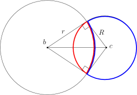
Figure III.1.4. The sphere $\mathbb{S}_{d-1}(c,R)$ maps to itself under inversion through $\mathbb{S}_{d-1}(b,r)$ provided the former is orthogonal to the latter, which is equivalent to $r^{2}+R^{2}=|c-b|^{2}$. In particular, the area contained in the blue segment (the crescent containing $c$) is mapped to the area in the red segment (the remainder of the ball centred at $c$) and vice versa.

We note in particular that $\mathbb{S}^{*}_{d}(c,R)=\mathbb{S}_{d-1}(c,R)$ if and only if $\lambda=1$, in other words, $r^{2}+R^{2}=|c-b|^{2}$. This is equivalent to requiring that the spheres $\mathbb{S}_{d-1}(c,R)$ and $\mathbb{S}_{d-1}(b,r)$ are orthogonal, and therefore necessarily overlapping. What is additionally interesting about this choice of $\mathbb{S}_{d-1}(c,R)$ is that its interior maps to its interior and its exterior to its exterior.

III.1.2. Inversions through another sphere with reflection

A variant of the transformation (102) takes the form

$$x^{\diamond}=b-\frac{r^{2}}{|x-b|^{2}}(x-b),$$ (106)

for a fixed $b\in\mathbb{R}^{d}$ and $x\in\mathbb{R}^{d}\backslash\{b\}$, which similarly has the self-inverse property (104). It is also quite straightforward to show that

$$r^{2}=|x^{\diamond}-b||x-b|$$ (107)

and

$$|x^{\diamond}-y^{\diamond}|=\frac{r^{2}|x-y|}{|x-b||y-b|}$$ (108)

still hold in the spirit of (103) and (105), respectively.

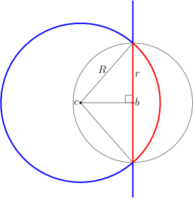
Figure III.1.5. The sphere $\mathbb{S}_{d-1}(c,R)$ maps to itself through $\mathbb{S}_{d-1}(b,r)$ via (106) providing $|c-b|^{2}+r^{2}=R^{2}$. However, this time, the exterior of the sphere $\mathbb{S}_{d-1}(c,R)$ maps to the interior of the sphere $\mathbb{S}_{d-1}(c,R)$ and vice versa. For example, the region in the exterior of $\mathbb{S}_{d-1}(c,R)$ contained by blue boundary (that is the half-space to the left of the vertical line excluding the intersection with the larger ball) maps to the portion of the interior of $\mathbb{S}_{d-1}(c,R)$ contained by the red boundary (that is the intersection of the larger ball with the half-space to the right of the vertical line).

Intuitively speaking $x^{\diamond}$ performs the same sphere inversion as $x^{*}$, albeit with the additional feature that there is pointwise reflection about $b$. As such, any sphere $\mathbb{S}_{d-1}(c,R)$ will map to another sphere, say $\mathbb{S}_{d-1}^{\diamond}(c,R)$ so long as $|c-b|<R$. We are again interested in choices of $c$ and $R$ such that $\mathbb{S}_{d-1}^{\diamond}(c,R)=\mathbb{S}_{d-1}(c,R)$. This turns out to be possible so long as $R^{2}=r^{2}+|c-b|^{2}$. Moreover, in that case, the interior of $\mathbb{S}_{d-1}(c,R)$ maps to its exterior and its exterior to its interior; see Fig. III.1.5.

To see how this is possible, we need to prove a new identity for $x^{\diamond}$. We claim that

$$|x^{\diamond}-c|^{2}-R^{2}=\frac{|x^{\diamond}-b|^{2}}{r}(R^{2}-|x-c|^{2}),\qquad x\in\mathbb{R}^{d}$$ (109)

Indeed, recalling that $|x^{\diamond}-b||x-b|=r^{2}$, we can write

$$x=b+\frac{(x-b)}{|x-b|}|x-b|\quad\text{ and }\quad x^{\diamond}=b-|x^{\diamond}-b|\frac{(x-b)}{|x-b|}.$$

Hence, as $|b-c|^{2}+r^{2}=R^{2}$ and using again that $|x^{\diamond}-b||x-b|=r^{2}$, we have

$$|x^{\diamond}-c|^{2}-R^{2} =|(x^{\diamond}-b)+(b-c)|^{2}-R^{2}$$

$$=|x^{\diamond}-b|^{2}-2|x^{\diamond}-b|\frac{(x-b)\cdot(b-c)}{|x-b|}-r^{2}$$

$$=\frac{|x^{\diamond}-b|^{2}}{r^{2}}\left(r^{2}-2(x-b)\cdot(b-c)-|x-b|^{2}\right)$$

$$=\frac{|x^{\diamond}-b|^{2}}{r^{2}}\left(R^{2}-|b-c|^{2}-2|x-b|\frac{(x-b)}{|x-b|}\cdot(b-c)-|x-b|^{2}\right)$$

$$=\frac{|x^{\diamond}-b|^{2}}{r^{2}}\left(R^{2}-|x-c|^{2}\right),$$ (110)

which proves (109).

It is now immediately apparent that $|x^{\diamond}-c|^{2}<R^{2}$ if and only if $|x-c|^{2}>R^{2}$, and $|x^{\diamond}-c|^{2}=R^{2}$ if and only if $|x-c|^{2}=R^{2}$ which is to say that $\mathbb{S}_{d-1}^{\diamond}(c,R)=\mathbb{S}_{d-1}(c,R)$ and that the interior of $\mathbb{S}_{d-1}(c,R)$ maps to its exterior and its exterior maps to its interior as claimed.

III.2. First hitting of the unit sphere

Let us turn to the first of two natural first passage problems that we will consider in this chapter. This concerns the distribution of the position of $X$ on first hitting of the sphere $\mathbb{S}_{d-1}=\{x\in\mathbb{R}^{d}:|x|=1\}$. To this end, let us introduce the notation

$$\tau^{\odot}=\inf\{t>0:|X_{t}|=1\}.$$

Theorem III.2.1 ($\heartsuit$).

Define the function

$$h^{\odot}(x,y)=\frac{\Gamma\left(\frac{\alpha+d}{2}-1\right)\Gamma\left(\frac{\alpha}{2}\right)}{\Gamma\left(\frac{d}{2}\right)\Gamma(\alpha-1)}\frac{||x|^{2}-1|^{\alpha-1}}{|x-y|^{\alpha+d-2}}$$

for $|x|\neq 1$, $|y|=1$. Then, if $\alpha\in(1,2)$,

$$\mathbb{P}_{x}(X_{\tau^{\odot}}\in{\textnormal{d}}y)=h^{\odot}(x,y)\sigma_{1}({\textnormal{d}}y)\mathbf{1}_{(|x|\neq 1)}+\delta_{x}({\textnormal{d}}y)\mathbf{1}_{(|x|=1)},\qquad|y|=1,$$

where $\sigma_{1}({\textnormal{d}}y)$ is the surface measure on $\mathbb{S}_{d-1}$, normalised to have unit total mass. Otherwise, if $\alpha\in(0,1]$, $\mathbb{P}_{x}(\tau^{\odot}=\infty)=1$, for all $|x|\neq 1$.

This theorem is due to Port (1969) and we largely follow his steps to its proof, with some adaptations to our updated point of view. Before proving it, we need to address a number of preliminary results first.

III.2.1. Probability of ever hitting $\mathbb{S}_{d-1}$

As alluded to above, the next result is due to Port (1969), albeit that we have opted to write the computed probability in terms of the hypergeometric function, ${}_{2}F_{1}$, rather than Port’s original choice, the Legendre function of the first kind. This is a consequence of our choice to re-prove his result using the perspective of a stable processes as a self-similar Markov process.

Theorem III.2.2 ($\diamondsuit$).

For $|x|>0$, if $\alpha\in(1,2)$, then

$$\mathbb{P}_{x}(\tau^{\odot}<\infty)$$

$$=\frac{\Gamma\left(\frac{\alpha+d}{2}-1\right)\Gamma\left(\frac{\alpha}{2}\right)}{\Gamma\left(\frac{d}{2}\right)\Gamma(\alpha-1)}\left\{\begin{array}[]{rl}{{}_{2}F_{1}((d-\alpha)/2,1-\alpha/2,d/2;|x|^{2})}&1>|x|\\ &\\ |x|^{\alpha-d}{{}_{2}F_{1}((d-\alpha)/2,1-\alpha/2,d/2;|x|^{-2})}&1\leq|x|.\end{array}\right.$$

Otherwise, if $\alpha\in(0,1]$, then $\mathbb{P}_{x}(\tau^{\odot}=\infty)=1$ for all $|x|\neq 1$.

Proof ($\clubsuit$).

From Secion I.2.4, we know that $|X|$ is a positive self-similar Markov process. Denote the underlying Lévy processes associated through the Lamperti transform by $\xi$ with probabilities $\mathbf{P}_{x}$, $x\in\mathbb{R}$.

$$\mathbb{P}_{x}(\tau^{\odot}<\infty)=\mathbf{P}_{\log|x|}(\tau^{\{0\}}<\infty)=\mathbf{P}_{0}(\tau^{\{\log(1/|x|)\}}<\infty),$$

where $\tau^{\{z\}}=\inf\{t>0:\xi_{t}=z\}$, $z\in\mathbb{R}$. From this observation, we note the ability of $X$ to hit the sphere $\mathbb{S}_{d-1}$ with positive probability, boils down to the ability of $\xi$ to hit points with positive probability. In this respect, classical theory of Lévy processes comes to our rescue again and II.Theorem 16 of Bertoin (1996) tells us that a necessary and sufficient condition boils down to the integrability of $(1+\Psi(z))^{-1}$, where $\Psi$ is the characteristic exponent of $\xi$, given by Theorem I.2.5.

Another important asymptotic relation for the gamma function that can be derived from Stirling’s formula states that, asymptotically as $y\to\infty$, for $x\in{\mathbb{R}}$,

$$|\Gamma(x+{\textnormal{i}}y)|=\sqrt{2\pi}e^{-\frac{\pi}{2}|y|}|y|^{x-\frac{1}{2}}(1+o(1)),$$ (111)

uniformly in any finite interval $-\infty<a\leq x\leq b<\infty$. Hence, appealing to (111),

$$\frac{1}{\Psi(z)}=\frac{\Gamma(-\frac{1}{2}{\rm i}z)}{\Gamma(\frac{1}{2}(-{\rm i}z+\alpha))}\frac{\Gamma(\frac{1}{2}({\rm i}z+d-\alpha))}{\Gamma(\frac{1}{2}({\rm i}z+d))}\sim|z|^{-\alpha}$$ (112)

uniformly on $\mathbb{R}$ as $|z|\to\infty$. We thus conclude that $(1+\Psi(z))^{-1}$ is integrable and each sphere $\mathbb{S}_{d-1}$ can be reached with positive probability from any $x$ with $|x|\neq 1$ if and only if $\alpha\in(1,2)$. Moreover, when $\alpha\in(1,2)$, Corollary II.18 of Bertoin (1996) again gives us the identity

$$\mathbb{P}_{x}(\tau^{\odot}<\infty)=\frac{u_{\xi}(\log(1/|x|))}{u_{\xi}(0)},$$ (113)

where, up to a multiplicative constant, the potential density $u_{\xi}$ can be computed via a Laplace inversion in the spirit of the computations completed in the proof of Theorem II.4.1.

To this end, we note that the Laplace exponent of $\xi$, $\Psi(-{\rm i}z)$, is well defined for ${\rm Re}(z)\in(-d,\alpha)$ with roots at $0$ and $\alpha-d$. The transience of $X$ for $d\geq 2$ ensures that $\mathbf{E}[\xi_{1}]>0$ and hence, as $-\Psi(-{\rm i}z)$ is convex for real $z$, we easily deduce that ${\rm Re}(\Psi(-{\rm i}z))>0$ for ${\rm Re}(z)\in(\alpha-d,0)$. In particular, it follows that the Laplace transform of $u_{\xi}$ is well defined for ${\rm Re}(z)\in(\alpha-d,0)$ as

$$\int_{{\mathbb{R}}}{\rm e}^{zx}u_{\xi}(x){\textnormal{d}}x=\int_{0}^{\infty}{\rm e}^{-\Psi(-{\rm i}z)t}{\textnormal{d}}t=\frac{1}{\Psi(-{\rm i}z)}.$$

As a consequence we can compute $u_{\xi}$ as a Laplace inversion in the form

$$u_{\xi}(x)=\frac{1}{2\pi{\rm i}}\int_{c+{\rm i}{\mathbb{R}}}\frac{{\rm e}^{-zx}}{{\Psi(-{\rm i}z)}}{\textnormal{d}}z,\qquad x\in\mathbb{R},$$

providing $c\in(\alpha-d,0)$.

As we have seen in the computation of (93), this integral can be computed using relatively straightforward residue calculus. Indeed, from (112) we note that $1/\Psi(-{\rm i}z)$ has simple poles at $\{2n,n\geq 0\}$, and $\{-2n-(d-\alpha):n\geq 0\}$.

We can construct a contour integral, $\gamma_{R}=\{c+{\rm i}x:|x|\leq R\}\cup\{c+R{\rm e}^{{\rm i}\theta}:\theta\in(\pi/2,3\pi/2)\}$, where $c\in(\alpha-d,0)$; see Fig. III.2.6.

Figure III.2.6. The contour integral $\gamma_{R}$.

Residue calculus now gives us

$$\frac{1}{2\pi{\rm i}}\int_{c-{\rm i}R}^{c+{\rm i}R}\frac{{\rm e}^{-zx}}{{\Psi(-{\rm i}z)}}{\textnormal{d}}z$$

$$\hskip 28.45274pt=-\frac{1}{2\pi{\rm i}}\int_{c+R{\rm e}^{{\rm i}\theta}:\theta\in(\pi/2,3\pi/2)}\frac{{\rm e}^{-zx}}{{\Psi(-{\rm i}z)}}{\textnormal{d}}z$$

$$\hskip 56.9055pt+\sum_{1\leq n\leq\lfloor R\rfloor}{\rm Res}\left(\frac{{\rm e}^{-zx}}{\Psi(-{\rm i}z)};z=-2n-(d-\alpha)\right).$$ (114)

Now fix $x\leq 0$. Appealing again to the uniform estimate (111), the assumption $x\leq 0$ and the fact that the arc length of $\{c+R{\rm e}^{{\rm i}\theta}:\theta\in(\pi/2,3\pi/2)\}$ is $\pi R$, we have

$$\left|\int_{c+R{\rm e}^{{\rm i}\theta}:\theta\in(\pi/2,3\pi/2)}\frac{{\rm e}^{-xz}}{\Psi(-{\rm i}z)}{\rm d}z\right|\leq CR^{-(\alpha-1)}\rightarrow 0$$

as $R\rightarrow\infty$ for some constant $C>0$. By taking limits in (114), we now have

$$u_{\xi}(x)=\sum_{n\geq 1}{\rm Res}\left(\frac{{\rm e}^{-zx}}{\Psi(-{\rm i}z)};z=-2n-(d-\alpha)\right).$$ (115)

Using the residues of the gamma function, that is, for $n=0,1,\cdots$, ${\rm Res}(\Gamma(z);z=-n)=(-1)^{n}/n!$, we have in (115), for $x\leq 0$,

$$u_{\xi}(x) =\sum_{0}^{\infty}(-1)^{n+1}\frac{\Gamma(n+(d-\alpha)/2)}{\Gamma(-n+\alpha/2)\Gamma(n+d/2)}\frac{{\rm e}^{2nx}}{n!}$$

$$={\rm e}^{x(d-\alpha)}\frac{\Gamma((d-\alpha)/2)}{\Gamma(\alpha/2)\Gamma(d/2)}\sum_{0}^{\infty}\frac{((d-\alpha)/2)_{n}(1-\alpha/2)_{n}}{(d/2)_{n}}\frac{{\rm e}^{2nx}}{n!}$$

$$={\rm e}^{x(d-\alpha)}\frac{\Gamma((d-\alpha)/2)}{\Gamma(\alpha/2)\Gamma(d/2)}{{}_{2}F_{1}((d-\alpha)/2,1-\alpha/2,d/2;{\rm e}^{2x})}$$ (116)

where $(a)_{n}=\Gamma(n+a)/\Gamma(a)$ is the Pochhammer symbol and we have used the relation

$$\Gamma(-n+x)=(-1)^{n-1}\frac{\Gamma(-x)\Gamma(1+x)}{\Gamma(n+1-x)},\qquad n\in\mathbb{N}$$

and the recursion formula for gamma functions.

Note in particular, this tells us that

$$u_{\xi}(0) =\frac{\Gamma((d-\alpha)/2)}{\Gamma(\alpha/2)\Gamma(d/2)}{{}_{2}F_{1}((d-\alpha)/2,1-\alpha/2,d/2;1)}$$

$$=\frac{\Gamma((d-\alpha)/2)}{\Gamma(\alpha/2)\Gamma(d/2)}\frac{\Gamma(d/2)\Gamma(\alpha-1)}{\Gamma(\alpha/2)\Gamma((\alpha+d)/2-1)}$$

Feeding (116) back in (113), we have thus established an identity for $\mathbb{P}_{x}(\tau^{\odot}<\infty)$ when $1\leq|x|$. To deal with the case $1>|x|$, we can appeal to the Riesz–Bogdan–Żak transform to help us. To this end we note that, for $|x|<1$,

$$\mathbb{P}_{x/|x|^{2}}(\tau^{\odot}<\infty)=\mathbb{E}_{x}\left[\frac{|X_{\tau^{\odot}}|^{\alpha-d}}{|x|^{\alpha-d}}\mathbf{1}_{(\tau^{\odot}<\infty)}\right]=\frac{1}{|x|^{\alpha-d}}\mathbb{P}_{x}(\tau^{\odot}<\infty)$$

and hence,

$$\mathbb{P}_{x}(\tau^{\odot}<\infty)=\frac{\Gamma\left(\frac{\alpha+d}{2}-1\right)\Gamma\left(\frac{\alpha}{2}\right)}{\Gamma\left(\frac{d}{2}\right)\Gamma(\alpha-1)}{{}_{2}F_{1}((d-\alpha)/2,1-\alpha/2,d/2;|x|^{2})},$$

thus completing the proof. ∎

III.2.2. Some Riesz potentials on $\mathbb{S}_{d-1}$

We continue our analysis, working towards the proof of Theorem III.2.1, keeping close to the steps in Port (1969). The proof of the next theorem is nonetheless new.

Theorem III.2.3 ($\heartsuit$).

Suppose $\alpha\in(1,2)$. For all $x\in\mathbb{R}^{d}$,

$$\mathbb{P}_{x}(\tau^{\odot}<\infty)=\frac{\Gamma\left(\frac{\alpha+d}{2}-1\right)\Gamma\left(\frac{\alpha}{2}\right)}{\Gamma\left(\frac{d}{2}\right)\Gamma(\alpha-1)}\int_{\mathbb{S}_{d-1}}|z-x|^{\alpha-d}\sigma_{1}({\textnormal{d}}z).$$ (117)

In particular, for $y\in\mathbb{S}_{d-1}$,

$$\int_{\mathbb{S}_{d-1}}|z-y|^{\alpha-d}\sigma_{1}({\textnormal{d}}z)=\frac{\Gamma\left(\frac{d}{2}\right)\Gamma(\alpha-1)}{\Gamma\left(\frac{\alpha+d}{2}-1\right)\Gamma\left(\frac{\alpha}{2}\right)}.$$ (118)

Proof ($\clubsuit$).

We start by recalling from (59) and Proposition I.3.14 that, for all $z\in\mathbb{R}^{d}$,

$$|X_{t}-z|^{\alpha-d},\qquad t\geq 0,$$

is a martingale. Indeed, note that for $x\neq 0$, $z\in\mathbb{R}^{d}$,

$$\mathbb{E}_{x}[|X_{t}-z|^{\alpha-d}]=\mathbb{E}_{x-z}[|X_{t}|^{\alpha-d}]=|x-z|^{\alpha-d},$$

where we have used that $(|X_{t}|^{\alpha-d},t\geq 0)$ is a martingale. As a consequence, we note that, for $0\leq s\leq t$,

$$\mathbb{E}_{x}\left[\left.\int_{\mathbb{S}_{d-1}}|z-X_{t\wedge\tau^{\odot}}|^{\alpha-d}\sigma_{1}({\textnormal{d}}z)\right|{\mathcal{F}_{s}}\right] =\int_{\mathbb{S}_{d-1}}\mathbb{E}_{x}\left[\left.|z-X_{t\wedge\tau^{\odot}}|^{\alpha-d}\right|{\mathcal{F}_{s}}\right]\sigma_{1}({\textnormal{d}}z)$$

$$=\int_{\mathbb{S}_{d-1}}|z-X_{s\wedge\tau^{\odot}}|^{\alpha-d}\sigma_{1}({\textnormal{d}}z),$$

thereby suggesting that

$$M_{t}:=\int_{\mathbb{S}_{d-1}}|z-X_{t\wedge\tau^{\odot}}|^{\alpha-d}\sigma_{1}({\textnormal{d}}z),\qquad t\geq 0,$$

is a martingale. Recalling that $X$ is transient in the sense that $\lim_{t\to\infty}|X_{t}|=\infty$, we note that, since $d\geq 2>\alpha$, on the event $\{\tau^{\odot}=\infty\}$,

$$\lim_{t\to\infty}\int_{\mathbb{S}_{d-1}}|z-X_{t\wedge\tau^{\odot}}|^{\alpha-d}\sigma_{1}({\textnormal{d}}z)=0.$$

Hence $(M_{t},t\geq 0)$ is uniformly integrable with almost sure limit

$$M_{\infty}:=\lim_{t\to\infty}M_{t}=\int_{\mathbb{S}_{d-1}}|z-X_{\tau^{\odot}}|^{\alpha-d}\sigma_{1}({\textnormal{d}}z)\mathbf{1}_{(\tau^{\odot}<\infty)}\stackrel{{\scriptstyle d}}{{=}}C\mathbf{1}_{(\tau^{\odot}<\infty)},$$

where, despite the randomness in $X_{\tau^{\odot}}$, by rotational symmetry,

$$C=\int_{\mathbb{S}_{d-1}}|z-{\texttt{1}}|^{\alpha-d}\sigma_{1}({\textnormal{d}}z),$$ (119)

and ${\texttt{1}}=(1,0,\cdots,0)\in\mathbb{R}^{d}$ is the ‘North Pole’ on $\mathbb{S}_{d-1}$. Note, it is not too difficult to see that $C$ is finite.

Preservation of martingale expectation for our martingale now ensures that

$$C\mathbb{P}_{x}(\tau^{\odot}<\infty)=\int_{\mathbb{S}_{d-1}}|z-x|^{\alpha-d}\sigma_{1}({\textnormal{d}}z).$$

and hence taking the limit as $|x|\to 0$, noting the right hand side above tends to unity, rotational symmetry and (119) ensures that, for all $y$ such that $|y|=1$,

$$C=\int_{\mathbb{S}_{d-1}}|z-y|^{\alpha-d}\sigma_{1}({\textnormal{d}}z)=\frac{1}{\mathbb{P}(\tau^{\odot}<\infty)}.$$

Thanks to scaling and Theorem III.2.2, it is clear that

$$\mathbb{P}(\tau^{\odot}<\infty)=\frac{\Gamma\left(\frac{\alpha+d}{2}-1\right)\Gamma\left(\frac{\alpha}{2}\right)}{\Gamma\left(\frac{d}{2}\right)\Gamma(\alpha-1)},$$

which completes the proof. ∎

The next result identifies the unique solution to a fixed point Riesz potential equation as the probability distribution that appears in Theorem III.2.1. It is a key step in Port (1969), but also in other works pertaining to first passage problems for stable processes during this era (as indeed we shall see in forthcoming sections); see e.g. Ray (1958) for its application in even earlier work, not to mention in the original work of Riesz (1938). We have also taken inspiration from Bliedtner and Hansen (1986).

Lemma III.2.4 ($\heartsuit$).

Suppose that $\alpha\in(1,2)$. Write $\mu^{\odot}_{x}({\textnormal{d}}z)=\mathbb{P}_{x}(X_{\tau^{\odot}}\in{\textnormal{d}}z)$ on $\mathbb{S}_{d-1}$ where $x\in\mathbb{R}^{d}\backslash\mathbb{S}_{d-1}$. Then the measure $\mu_{x}^{\odot}$ is the unique solution to

$$|x-y|^{\alpha-d}=\int_{\mathbb{S}_{d-1}}|z-y|^{\alpha-d}\mu({\textnormal{d}}z),\qquad y\in\mathbb{S}_{d-1}.$$ (120)

Proof ($\heartsuit$).

We begin by recalling the expression for the potential of the stable process in Theorem I.1.6 which states that, due to transience,

$$\int_{0}^{\infty}\mathbb{P}_{x}(X_{t}\in{\textnormal{d}}y){\textnormal{d}}t=C(\alpha)|x-y|^{\alpha-d}{\textnormal{d}}y,\qquad x,y\in\mathbb{R}^{d},$$

where $C(\alpha)$ is an unimportant constant in the following discussion. Suppose now that we fix an arbitrary $y\in\mathbb{S}_{d-1}$. Then a straightforward application of the Strong Markov Property tells us that, for $x\in\mathbb{R}^{d}\backslash\mathbb{S}_{d-1}$,

$$\int_{0}^{\infty}\mathbb{P}_{x}(X_{t}\in{\textnormal{d}}y){\textnormal{d}}t =\mathbb{E}_{x}\left[\mathbf{1}_{(\tau^{\odot}<\infty)}\int_{0}^{\infty}\mathbb{P}_{z}(X_{t}\in{\textnormal{d}}y)|_{z=X_{\tau^{\odot}}}{\textnormal{d}}t\right]$$

$$=\mathbb{E}_{x}\left[\mathbf{1}_{(\tau^{\odot}<\infty)}C(\alpha)|X_{\tau^{\odot}}-y|^{\alpha-d}\right]{\textnormal{d}}y$$

$$=C(\alpha)\int_{\mathbb{S}_{d-1}}|z-y|^{\alpha-d}\mathbb{P}_{x}(X_{\tau^{\odot}}\in{\textnormal{d}}z){\textnormal{d}}y,$$

which shows that $\mu_{x}^{\odot}$ is a solution to (120).

Let us now address the issue of uniqueness in (131). If $\mu({\textnormal{d}}y)$ is any other probability measure supported on $\mathbb{S}_{d-1}$, then, for $|x|\neq 1$,

$$\int_{\mathbb{S}_{d-1}}\int_{\mathbb{S}_{d-1}}|z-y|^{\alpha-d}\mu^{\odot}_{x}({\textnormal{d}}z)\mu({\textnormal{d}}y)=\int_{\mathbb{S}_{d-1}}|x-y|^{\alpha-d}\mu({\textnormal{d}}y)\leq(1+|x|)^{\alpha-d},$$

where we have used rotational symmetry in the second equality so that the largest value the integrand can take occurs when $y=x/|x|$.

Now suppose that $\nu$ is a signed measure on $\mathbb{S}_{d-1}$ which satisfies

$$\int_{\mathbb{S}_{d-1}}\int_{\mathbb{S}_{d-1}}|z-y|^{\alpha-d}\,|\nu|({\textnormal{d}}z)\,|\nu|({\textnormal{d}}y)<\infty.$$

Here, we understand $|\nu|=\nu^{+}+\nu^{-}$, when we represent $\nu=\nu^{+}-\nu^{-}$. We claim that

$$\int_{\mathbb{S}_{d-1}}|z-y|^{\alpha-d}\nu({\textnormal{d}}z)=0$$ (121)

implies that the measure $\nu\equiv 0$. The significance of this claim is that it would immediately imply that (120) has a unique solution in the class of probability measures.

Verifying the claim (121) is not too difficult. Indeed, if we write $\texttt{p}(z,t)$ for the transition density of $X$, that is, $\mathbb{P}_{x}(X_{t}\in{\textnormal{d}}y)=\texttt{p}(y-x,t){\textnormal{d}}y$, then a standard Fourier inverse tells us that, for $x\in\mathbb{R}^{d}$,

$$\texttt{p}(x,t)=(2\pi)^{-d}\int_{\mathbb{R}^{d}}{\rm e}^{{\rm i}\theta\cdot x}{\rm e}^{-|\theta|^{\alpha}t}{\textnormal{d}}\theta.$$

note that

$$C(\alpha)\int_{\mathbb{S}_{d-1}}\int_{\mathbb{S}_{d-1}}|z-y|^{\alpha-d}\,\nu({\textnormal{d}}z)\,\nu({\textnormal{d}}y)$$

$$\hskip 28.45274pt=\int_{\mathbb{S}_{d-1}}\int_{\mathbb{S}_{d-1}}\int_{0}^{\infty}\texttt{p}(z-y,t)\,{\textnormal{d}}t\,\nu({\textnormal{d}}z)\,\nu({\textnormal{d}}y)$$

$$\hskip 28.45274pt=\int_{\mathbb{S}_{d-1}}\int_{\mathbb{S}_{d-1}}\int_{0}^{\infty}(2\pi)^{-d}\int_{\mathbb{R}^{d}}{\rm e}^{{\rm i}\theta\cdot(z-y)}{\rm e}^{-|\theta|^{\alpha}t}{\textnormal{d}}\theta\,{\textnormal{d}}t\,\nu({\textnormal{d}}z)\,\nu({\textnormal{d}}y)$$

$$\hskip 28.45274pt=(2\pi)^{-d}\int_{0}^{\infty}{\textnormal{d}}t\int_{\mathbb{R}^{d}}{\textnormal{d}}\theta\,{\rm e}^{-|\theta|^{\alpha}t}\left(\int_{\mathbb{S}_{d-1}}{\rm e}^{-{\rm i}\theta\cdot y}\nu({\textnormal{d}}y)\right)\left(\int_{\mathbb{S}_{d-1}}{\rm e}^{{\rm i}\theta\cdot z}\nu({\textnormal{d}}z)\right)$$

$$\hskip 28.45274pt=(2\pi)^{-d}\int_{0}^{\infty}{\textnormal{d}}t\int_{\mathbb{R}^{d}}{\textnormal{d}}\theta\,{\rm e}^{-|\theta|^{\alpha}t}|\phi(\theta)|^{2},$$

where $\phi(\theta)=\int_{\mathbb{S}_{d-1}}{\rm e}^{{\rm i}\theta\cdot z}\nu({\textnormal{d}}z)$. The assumption that $\int_{\mathbb{S}_{d-1}}|z-y|^{\alpha-d}\nu({\textnormal{d}}z)=0$ thus implies that $\phi\equiv 0$, which, in turn, implies $\nu\equiv 0$, as claimed, and hence (120) has a unique solution. ∎

III.2.3. Distribution of hitting location on $\mathbb{S}_{d-1}$

Proof of Theorem III.2.1 ($\heartsuit$).

We only prove the first part of the theorem. The last part has been established in Theorem III.2.2.

First assume that $|x|>1$. Starting with the equality (118) we want to apply the transformation (102) through the sphere $\mathbb{S}_{d-1}(x,(|x|^{2}-1)^{1/2})$ remembering that this transformation maps $\mathbb{S}_{d-1}$ to itself. From Blumenson (1960) we know that, if we write $y=rA(\theta)$, where $r=|y|>0$ and $A(\theta)={\rm Arg}(y)$ for parameterisation $\theta=(\theta_{1},\cdots,\theta_{d-1})$, where $\theta_{j}\in[0,\pi]$ and $\theta_{d-1}\in[0,2\pi)$ then

$${\textnormal{d}}y=r^{d-1}\mathcal{J}(\theta){\textnormal{d}}\theta{\textnormal{d}}r=\frac{2\pi^{d/2}}{\Gamma(d/2)}r^{d-1}\sigma_{1}({\textnormal{d}}y){\textnormal{d}}r,$$ (122)

where $\mathcal{J}$ is the part of the Jacobian of $y$ with respect to $(r,\theta)$ which depends on $\theta$ and $\sigma_{1}({\textnormal{d}}y)$ is the surface measure on $\mathbb{S}_{d-1}$ normalised to have unit mass. Suppose now that we write $z=wA(\theta)$ and set $y=Kz=w^{-1}A(\theta)$, then, if we set $r=w^{-1}$,

$${\textnormal{d}}y=\left.r^{d-1}\mathcal{J}(\theta)\right|_{r=w^{-1}}{\textnormal{d}}\theta\frac{{\textnormal{d}}r}{{\textnormal{d}}w}{\textnormal{d}}w=w^{-2d}\cdot w^{d-1}\mathcal{J}(\theta){\textnormal{d}}w{\textnormal{d}}\theta=|z|^{-2d}{\textnormal{d}}z.$$ (123)

Now taking account of the fact that, transforming through the sphere $\mathbb{S}_{d-1}(x,(|x|^{2}-1)^{1/2})$, $z^{*}=x+K\tilde{z}$, where $\tilde{z}=(1-|x|^{2})^{-1}(z-x)$, we can work with the change of variables

$${\textnormal{d}}z^{*}=(|x|^{2}-1)^{2d}|z-x|^{-2d}\prod_{i=1}^{d}\frac{{\textnormal{d}}z_{i}}{(|x|^{2}-1)}=(|x|^{2}-1)^{d}|z-x|^{-2d}{\textnormal{d}}z,$$ (124)

where $z=(z_{1},\cdots,z_{d})$. In particular, appealing to (122) and (105), this tells us that, using obvious notation,

$$\frac{2\pi^{d/2}}{\Gamma(d/2)}(r^{*})^{d-1}\sigma_{1}({\textnormal{d}}z^{*}){\textnormal{d}}r^{*}=\left\{\frac{2\pi^{d/2}}{\Gamma(d/2)}\frac{(|x|^{2}-1)^{d-1}}{|z-x|^{2d-2}}r^{d-1}\sigma_{1}({\textnormal{d}}z)\right\}\left\{\frac{(|x|^{2}-1)}{|z-x|^{2}}{\textnormal{d}}r\right\}.$$

In particular, since $|z|^{*}=1$ if and only if $|z|=1$, the change of variable in the surface measure $\sigma_{1}$ satisfies

$$\sigma_{1}({\textnormal{d}}z^{*})=\frac{(|x|^{2}-1)^{d-1}}{|z-x|^{2d-2}}\sigma_{1}({\textnormal{d}}z),\qquad z\in\mathbb{S}_{d-1}.$$

Taking account of (103), this can equivalently be written as

$$\frac{1}{|z^{*}-x|^{d-1}}\sigma_{1}({\textnormal{d}}z^{*})=\frac{1}{|z-x|^{d-1}}\sigma_{1}({\textnormal{d}}z),\qquad z\in\mathbb{S}_{d-1}.$$ (125)

Returning to (118), with the help of (105) and (103) for the transformation (102) in $\mathbb{S}_{d-1}(x,(|x|^{2}-1)^{1/2})$ and (125), this gives us for $x\in\mathbb{R}^{d}\backslash\mathbb{S}_{d-1}$ and $y\in\mathbb{S}_{d-1}$,

$$\frac{\Gamma\left(\frac{d}{2}\right)\Gamma(\alpha-1)}{\Gamma\left(\frac{\alpha+d}{2}-1\right)\Gamma\left(\frac{\alpha}{2}\right)} =\int_{\mathbb{S}_{d-1}}|z^{*}-x|^{d-1}|z^{*}-y^{*}|^{\alpha-d}\frac{\sigma_{1}({\textnormal{d}}z^{*})}{|z^{*}-x|^{d-1}}$$

$$=\frac{(|x|^{2}-1)^{\alpha-1}}{|y-x|^{\alpha-d}}\int_{\mathbb{S}_{d-1}}\frac{|z-y|^{\alpha-d}}{|z-x|^{\alpha+d-2}}\sigma_{1}({\textnormal{d}}z).$$ (126)

Which is to say

$$|x-y|^{\alpha-d}=\int_{\mathbb{S}_{d-1}}|z-y|^{\alpha-d}\frac{\Gamma\left(\frac{\alpha+d}{2}-1\right)\Gamma\left(\frac{\alpha}{2}\right)}{\Gamma\left(\frac{d}{2}\right)\Gamma(\alpha-1)}\frac{(|x|^{2}-1)^{\alpha-1}}{|z-x|^{\alpha+d-2}}\sigma_{1}({\textnormal{d}}z),$$

which by uniqueness given in Lemma III.2.4 establishes the statement of the theorem for $|x|>1$.

Finally for the case $|x|<1$, we can appeal to similar reasoning albeit now using $x^{\diamond}$ to invert through the sphere $\mathbb{S}_{d-1}(x,(1-|x|^{2})^{1/2})$. The details are left to the reader. ∎

Remark III.2.5.

Although we have excluded the setting of Brownian motion, that is, the case $\alpha=2$, our analysis can be easily adapted to include it. In that case, the conclusion of Theorems III.2.1 and III.2.2 provide us with the classical Newtonian Poisson potential formula. Indeed, for $|x|<1$,

$$\mathbb{P}_{x}(X_{\tau^{\odot}}<\infty)=1=\int_{\mathbb{S}_{d-1}}\frac{(1-|x|^{2})}{|z-x|^{d}}\sigma_{1}({\textnormal{d}}z).$$ (127)

Similarly we can also reproduce the classical conclusion that, for $|x|>1$,

$$\mathbb{P}_{x}(X_{\tau^{\odot}}<\infty)=|x|^{2-d}=\int_{\mathbb{S}_{d-1}}\frac{(|x|^{2}-1)}{|z-x|^{d}}\sigma_{1}({\textnormal{d}}z).$$ (128)

III.2.4. Resolvent on $\mathbb{R}^{d}\backslash\mathbb{S}_{d-1}$

Write the associated potential measure as

$$U^{\odot}(x,{\textnormal{d}}y)=\int_{0}^{\infty}\mathbb{P}_{x}(X_{t}\in{\textnormal{d}}y,\,t<\tau^{\odot}){\textnormal{d}}t,\qquad x,y\in\mathbb{R}^{d}\backslash\mathbb{S}_{d-1}.$$

The next result again is taken from Port (1969). We follow the original proof, with some additional efficiencies introduced thanks to the Riesz–Bogdan–Żak transform.

Theorem III.2.6 ($\heartsuit$).

Suppose we write $Q(x)=\mathbb{P}_{x}(\tau^{\odot}<\infty)$, for $x\in\mathbb{R}^{d}$. Then, for all $x,y\in\mathbb{R}^{d}\backslash\mathbb{S}_{d-1}$,

$$U^{\odot}(x,{\textnormal{d}}y)=2^{-\alpha}\pi^{-d/2}\frac{\Gamma((d-\alpha)/2)}{\Gamma(\alpha/2)}|x-y|^{\alpha-d}\left(1-Q\left(\frac{y}{|y-x|}\left|x-\frac{y}{|y|^{2}}\right|\right)\right){\textnormal{d}}y.$$

Proof ($\diamondsuit$).

Let us preemptively assume that $U^{\odot}(x,{\textnormal{d}}y)$ has density with respect to Lebesgue measure, written $u^{\odot}(x,y)$, $x,y\in\mathbb{R}^{d}\backslash\mathbb{S}_{d-1}$. As alluded to above, straightforward path counting tells us that

$$u^{\odot}(x,y)=C_{\alpha}|x-y|^{\alpha-d}-C_{\alpha}\int_{\mathbb{S}_{d-1}}|z-y|^{\alpha-d}h^{\odot}(x,z)\sigma_{1}({\textnormal{d}}z),$$

where for convenience we have written $C_{\alpha}=2^{-\alpha}\pi^{-d/2}{\Gamma((d-\alpha)/2)}/{\Gamma(\alpha/2)}$. In order to deal with the integral on the right-hand side above, we need to split our computations into the cases that $|x|<1$ and $|x|>1$.

First assume that $|x|>1$. We appeal to a sphere inversion of the type (102) via the sphere $\mathbb{S}_{d-1}(x,(|x|^{2}-1)^{1/2})$ in a manner similar to the computation in (126). Indeed, reading only the second equality of (126), we see that

$$C_{\alpha}\int_{\mathbb{S}_{d-1}}|z-y|^{\alpha-d}h^{\odot}(x,z)\sigma_{1}({\textnormal{d}}z)$$

$$=C_{\alpha}\frac{\Gamma\left(\frac{\alpha+d}{2}-1\right)\Gamma\left(\frac{\alpha}{2}\right)}{\Gamma\left(\frac{d}{2}\right)\Gamma(\alpha-1)}|x-y|^{\alpha-d}\int_{\mathbb{S}_{d-1}}|z^{*}-y^{*}|^{\alpha-d}\sigma_{1}({\textnormal{d}}z^{*})$$

$$=C_{\alpha}|x-y|^{\alpha-d}Q(y^{*}),$$

where in the second equality above, we have used Theorem III.2.3. Recalling that $y^{*}=x+(|x|^{2}-1)(y-x)/|y-x|^{2}$, a straightforward piece of algebra tells us that

$$|y^{*}|^{2}|y-x|^{2}=|y|^{2}\left|x-\frac{y}{|y|^{2}}\right|^{2}$$

and the result follows as soon as we note that isometry implies that $Q(y^{*})=Q(|y^{*}|y/|y|)$.

For the case that $|x|<1$, we can again appeal to the Riesz–Bogdan–Żak transform. The time change (62) implies that if we write $s=\eta(t)$ in the aforesaid transform, then ${\rm d}s/{\textnormal{d}}t=|X_{s}|^{2\alpha}$. Together with the Doob $h$-transform (59), we have, for bounded measurable $f:\mathbb{R}^{d}\to\mathbb{R}^{d}$,

$$\int_{\mathbb{R}^{d}}f(y)\frac{|y|^{\alpha-d}}{|x|^{\alpha-d}}u^{\odot}(x,y){\textnormal{d}}y =\int_{0}^{\infty}\frac{|y|^{\alpha-d}}{|x|^{\alpha-d}}\mathbb{E}_{x}[f(X_{t});\,t<\tau^{\odot}]{\textnormal{d}}t$$

$$=\mathbb{E}^{\circ}_{x}\left[\int_{0}^{\infty}f(X_{t})\mathbf{1}_{(t<\tau^{\odot})}{\textnormal{d}}t\right]$$

$$=\mathbb{E}_{Kx}\left[\int_{0}^{\infty}f(KX_{s})\mathbf{1}_{(s<\tau^{\odot})}|X_{s}|^{-2\alpha}{\textnormal{d}}s\right]$$

$$=\int_{\mathbb{R}^{d}}f(Ky)|y|^{-2\alpha}u^{\odot}(Kx,y){\textnormal{d}}y$$

$$=\int_{\mathbb{R}^{d}}f(z)|z|^{2(\alpha-d)}u^{\odot}(Kx,Kz){\textnormal{d}}z,\qquad y\in\mathbb{R}^{d}\backslash\mathbb{S}_{d-1},$$

where we recall that $\mathbb{E}^{\circ}_{x}$ is expectation with respect to $\mathbb{P}^{\circ}_{x}$, which was defined in (46), that $Kx=x/|x|^{2}$ and we have used (123) in the final equaltiy. We can now appeal to the expression we have just derived for $u^{\odot}$ previously on account of the fact that $|Kx|=1/|x|>1$. Equation (105) for the transform $K$ tells us that $|Ky-Kx|=|x-y|/|x||y|$. Hence we have for $|x|<1$ and $y\in\mathbb{R}^{d}\backslash\mathbb{S}_{d-1}$,

$$u^{\odot}(x,y) =C_{\alpha}|x|^{\alpha-d}|y|^{\alpha-d}|Kx-Ky|^{\alpha-d}\left(1-Q\left(\frac{Ky}{|Ky-Kx|}\left|Kx-KKy\right|\right)\right)$$

$$=C_{\alpha}|x-y|^{\alpha-d}\left(1-Q\left(\frac{y}{|y-x|}\left|x-Ky\right|\right)\right)$$

as required. ∎

III.3. First entrance and exit of the unit ball

III.3.1. First passage laws for $\mathbb{B}_{d}$

Let us start by defining the stopping times

$$\tau^{\oplus}:=\inf\{t>0:|X_{t}|<1\}\text{ and }\tau^{\ominus}:=\inf\{t>0:|X_{t}|>1\}.$$

Recall that $X$ is transient in dimension $d\geq 2$ and hence $\mathbb{P}_{x}(\tau^{\oplus}<\infty)<1$ for all $|x|\geq 1$ and $\mathbb{P}_{x}(\tau^{\ominus}<\infty)=1$ for all $|x|\leq 1$.

Blumenthal et al. (1961) give the distribution of $X_{\tau^{\ominus}}$ and then use a transformation which is tantamount to that of Riesz–Bogdan–Żak, attributing their method to Riesz (1938), to give directly the distribution of $X_{\tau^{\oplus}}$. We state their result below.

Theorem III.3.1 ($\heartsuit$).

Define the function

$$g(x,y)=\pi^{-(d/2+1)}\,\Gamma(d/2)\,\sin(\pi\alpha/2)\frac{\left|1-|x|^{2}\right|^{\alpha/2}}{\left|1-|y|^{2}\right|^{\alpha/2}}|x-y|^{-d}$$

for $x,y\in\mathbb{R}^{d}\backslash\mathbb{S}_{d-1}$.

(i):

Suppose that $|x|<1$, then

$$\mathbb{P}_{x}(X_{\tau^{\ominus}}\in{\textnormal{d}}y)=g(x,y){\textnormal{d}}y,\qquad|y|\geq 1.$$ (129)

(ii):

Suppose that $|x|>1$, then

$$\mathbb{P}_{x}(X_{\tau^{\oplus}}\in{\textnormal{d}}y,\,\tau^{\oplus}<\infty)=g(x,y){\textnormal{d}}y,\qquad|y|\leq 1.$$ (130)

The fact that the Riesz–Bogdan–Żak transform lies behind the relationship between the distributions of $X_{\tau^{\ominus}}$ and $X_{\tau^{\oplus}}$ should reassure the reader that one uses a single density function to describe both laws. As we shall shortly see, this function is symmetric in relation to the sphere inversion $(x,y)\mapsto(Kx,Ky)$.

We follow the original steps of Blumenthal et al. (1961), first passing through an intermediate result, which mirrors the approach of Lemma III.2.4. We omit its proof as it follows an almost identical thread to that of Lemma III.2.4.

Lemma III.3.2 ($\heartsuit$).

We have that, for $|x|<1$, uniquely in the class of probability distributions supported on the exterior of $\mathbb{S}_{d-1}$, $\mu^{\ominus}_{x}({\textnormal{d}}z):=\mathbb{P}_{x}(X_{\tau^{\ominus}}\in{\textnormal{d}}z)$ solves

$$|x-y|^{\alpha-d}=\int_{|z|\geq 1}|z-y|^{\alpha-d}\mu({\textnormal{d}}z),\qquad|y|>1.$$ (131)

and, for $|x|>1$, again uniquely in the class of probability distributions supported on the interior of $\mathbb{S}_{d-1}$, $\mu^{\oplus}_{x}({\textnormal{d}}z):=\mathbb{P}_{x}(X_{\tau^{\oplus}}\in{\textnormal{d}}z,\,\tau^{\oplus}<\infty)$ uniquely solves

$$|x-y|^{\alpha-d}=\int_{|z|\leq 1}|z-y|^{\alpha-d}\mu({\textnormal{d}}z),\qquad|y|<1.$$ (132)

We now turn our attention to showing that the unique solution to (131) and (132) are given by $\mu^{\ominus}_{x}({\textnormal{d}}z)=g(x,z){\textnormal{d}}z$, $|z|>1>|x|$ and $\mu^{\oplus}({\textnormal{d}}z)=g(x,z){\textnormal{d}}z$, $|z|<1<|x|$.

Proof of Theorem III.3.1 (i) ($\heartsuit$).

The proof is complete as soon as we can verify that

$$|x-y|^{\alpha-d}=c_{\alpha,d}\int_{|z|\geq 1}|z-y|^{\alpha-d}\frac{|1-|x|^{2}|^{\alpha/2}}{|1-|z|^{2}|^{\alpha/2}}|x-z|^{-d}{\textnormal{d}}z$$ (133)

for $|y|>1>|x|$, where

$$c_{\alpha,d}=\pi^{-(1+d/2)}\,\Gamma(d/2)\,\sin(\pi\alpha/2).$$

Starting with the integral on the right-hand side of (133), we will appeal to the transformation (106) through the sphere $\mathbb{S}_{d-1}(x,(1-|x|^{2})^{1/2})$, noting in particular that

$$|z^{\diamond}-y^{\diamond}|=(1-|x|^{2})\frac{|z-y|}{|z-x||y-x|}\,\,\text{ and }\,\,|z|^{2}-1=\frac{|z-x|^{2}}{1-|x|^{2}}(1-|z^{\diamond}|^{2}),$$ (134)

where the second identity comes from (110). A similar analysis of the differential calculus associated to (106) gives us

$${\textnormal{d}}z^{\diamond}=(1-|x|^{2})^{d}|z-x|^{-2d}{\textnormal{d}}z,\qquad z\in\mathbb{R}^{d},$$ (135)

just as in (135).

Now we can use (134) and (135) to compute, for $|x|<1<|y|$,

$$c_{\alpha,d}\int_{|z|\geq 1}|z-y|^{\alpha-d}\frac{|1-|x|^{2}|^{\alpha/2}}{|1-|z|^{2}|^{\alpha/2}}|x-z|^{-d}{\textnormal{d}}z$$

$$=c_{\alpha,d}|y-x|^{\alpha-d}\int_{|z^{\diamond}|\leq 1}\frac{|z^{\diamond}-y^{\diamond}|^{\alpha-d}}{|1-|z^{\diamond}|^{2}|^{\alpha/2}}{\textnormal{d}}z^{\diamond}.$$ (136)

Next we perform another transformation of the type (106), albeit through the sphere $\mathbb{S}_{d-1}(y^{\diamond},(1-|y^{\diamond}|^{2})^{1/2})$. In a similar fashion to the calculation that led to the right-hand side of (136), using (107) and the second equality in (134) we obtain

$$c_{\alpha,d}\int_{|z|\geq 1}|z-y|^{\alpha-d}\frac{|1-|x|^{2}|^{\alpha/2}}{|1-|z|^{2}|^{\alpha/2}}|x-z|^{-d}{\textnormal{d}}z$$

$$=c_{\alpha,d}|y-x|^{\alpha-d}\int_{|w|\geq 1}\frac{|1-|y^{\diamond}|^{2}|^{\alpha/2}}{|1-|w|^{2}|^{\alpha/2}}|w-y^{\diamond}|^{-d}{\textnormal{d}}w.$$ (137)

The question now remains as to whether the integral on right-hand side of (137) is equal to $1/c_{\alpha,d}$. We resolve this issue by recalling that the surface volume/area of a sphere of radius $r$ is given by ${2\pi^{d/2}}r^{d-1}/{\Gamma(d/2)}$. Moreover, writing, for $|y^{\diamond}|<1$,

$$\int_{|w|\geq 1}\frac{1}{|1-|w|^{2}|^{\alpha/2}}|w-y^{\diamond}|^{-d}{\textnormal{d}}w$$

$$=\frac{2\pi^{d/2}}{\Gamma(d/2)}\int_{1}^{\infty}r^{d-1}{\textnormal{d}}r\int_{\mathbb{S}_{d-1}(0,r)}\frac{1}{|1-|z|^{2}|^{\alpha/2}}|z-y^{\diamond}|^{-d}\sigma_{r}({\textnormal{d}}z)$$

$$=\frac{2\pi^{d/2}}{\Gamma(d/2)}\int_{1}^{\infty}\frac{r^{d-1}{\textnormal{d}}r}{|1-r^{2}|^{\alpha/2}}\int_{\mathbb{S}_{d-1}(0,r)}|z-y^{\diamond}|^{-d}\sigma_{r}({\textnormal{d}}z),$$ (138)

where $\sigma_{r}({\textnormal{d}}z)$ is the surface measure on $\mathbb{S}_{d-1}(0,r)$, normalised to have unit total mass. In order to continue, we remind the reader of a classical integral identity from Newtonian $d$-dimensional potential theory. Specifically, the Poisson formula (127) gives us

$$\int_{\mathbb{S}_{d-1}(0,r)}\frac{r^{d-2}(r^{2}-|y^{\diamond}|^{2})}{|z-y^{\diamond}|^{d}}\sigma_{r}({\textnormal{d}}z)=1,\qquad|y^{\diamond}|<1<r.$$ (139)

(The reader will also note that the kernel in the integral above is the distribution of where a $d$-dimensional Brownian motion issued from $y^{\diamond}$ will hit the sphere $\mathbb{S}_{d-1}(0,r)$.)

The identity (139) allows us to continue to develop the right-hand side of (138) so that we have

$$\int_{|v|\geq 1}\frac{1}{|1-|w|^{2}|^{\alpha/2}}|w-y^{\diamond}|^{-d}{\textnormal{d}}w=\frac{\pi^{d/2}}{\Gamma(d/2)}\int_{1}^{\infty}\frac{2r}{(r^{2}-1)^{\alpha/2}(r^{2}-|y^{\diamond}|^{2})}{\textnormal{d}}r.$$ (140)

A further change of variable, first $s=(r^{2}-1)/(1-|y^{\diamond}|^{2})$ and the definition of the beta function

$$\int_{1}^{\infty}\frac{2r}{(r^{2}-1)^{\alpha/2}(r^{2}-|y^{\diamond}|^{2})}{\textnormal{d}}r =\frac{1}{(1-|y^{\diamond}|^{2})^{\alpha/2}}\int_{0}^{\infty}s^{-\alpha/2}(1+s)^{-1}{\textnormal{d}}s$$

$$=\frac{1}{(1-|y^{\diamond}|^{2})^{\alpha/2}}\Gamma(\alpha/2)\Gamma(1-\alpha/2)$$

$$=\frac{\pi}{\sin(\alpha\pi/2)}\frac{1}{(1-|y^{\diamond}|^{2})^{\alpha/2}}.$$

Plugging back into (140), and then into (137), we end up with

$$\int_{|z|\geq 1}|z-y|^{\alpha-d}\frac{|1-|x|^{2}|^{\alpha/2}}{|1-|z|^{2}|^{\alpha/2}}|x-z|^{-d}{\textnormal{d}}z=\frac{\pi^{1+d/2}}{\Gamma(d/2)\sin(\alpha\pi/2)}\\ =\frac{1}{c_{\alpha,d}}$$

as required.

The identity (133) is thus affirmed for all $|x|<1<|y|$ and hence the first part of Theorem III.3.1 is proved. ∎

Proof of Theorem III.3.1 (ii) ($\diamondsuit$).

We can appeal to the Riesz–Bogdan–Żak transform in Theorem I.3.16 and note that for Borel set $D\subseteq\{u:|u|\leq 1\}$ and $|x|>1$,

$$\mathbb{P}_{x}(X_{\tau^{\oplus}}\in D)=\mathbb{P}^{\circ}_{Kx}(KX_{\tau^{\ominus}}\in D),$$

where we recall that $Kx=x/|x|^{2}$, $KD=\{Kx:x\in D\}$ and $\mathbb{P}^{\circ}_{x}$, $x\neq 0$, is the result of the Doob $h$-transform in (59). It follows that

$$\mathbb{P}_{x}(X_{\tau^{\oplus}}\in D)$$

$$=\int_{KD}\frac{|y|^{\alpha-d}}{|Kx|^{\alpha-d}}g(Kx,y){\textnormal{d}}y$$

$$=c_{\alpha,d}\int_{KD}|z|^{d-\alpha}|Kx|^{d-\alpha}\frac{|1-|Kx|^{2}|^{\alpha/2}}{|1-|y|^{2}|^{\alpha/2}}|Kx-y|^{-d}{\textnormal{d}}y$$

$$=c_{\alpha,d}\int_{D}|z|^{2d}\frac{|1-|x|^{2}|^{\alpha/2}}{|1-|z|^{2}|^{\alpha/2}}|x-z|^{-d}{\textnormal{d}}(Kz),$$ (141)

where we have used the change of variable $y=Kz$ together with (105) in the final equality. Appealing to (123), we can now complete the computation in (141). We have

$$\mathbb{P}_{x}(X_{\tau^{\oplus}}\in D)=c_{\alpha,d}\int_{D}\frac{|1-|x|^{2}|^{\alpha/2}}{|1-|z|^{2}|^{\alpha/2}}|x-z|^{-d}{\textnormal{d}}z=\int_{D}g(x,z){\textnormal{d}}z,$$

as required. ∎

Recalling that in dimensions $d\geq 2$, the stable process is transient. It thus makes sense to compute the probability that the unit ball around the origin is never entered. That is to say, to compute the total mass of the measure $\mu^{\oplus}$. Naturally one can do this by marginalising the distribution density $g$, however it turns out to be simpler to make use of the Lamperti representation of $|X|$. We thus offer a new proof to a result of Blumenthal et al. (1961)

Lemma III.3.3 ($\heartsuit$).

We have for $|x|>1$,

$$\mathbb{P}_{x}(\tau^{\oplus}=\infty)=\frac{\Gamma(d/2)}{\Gamma((d-\alpha)/2)\Gamma(\alpha/2)}\int_{0}^{|x|^{2}-1}(u+1)^{-d/2}u^{\alpha/2-1}{\textnormal{d}}u.$$

Proof ($\clubsuit$).

From Theorem I.2.5 we have the Wiener–Hopf factorisation of the characteristic exponent of $\xi$, the Lévy process appearing in the Lamperti transform of $|X|$. In particular, its descending ladder height process has Laplace exponent given by ${\Gamma((\lambda+\alpha)/2)}/{\Gamma(\lambda/2)}$, $\lambda\geq 0$. If we denote its descending ladder height potential measure by $\hat{U}_{\xi}$, then, from the discussion following (69), we have that

$$\int_{[0,\infty)}{\rm e}^{-\lambda x}\hat{U}_{\xi}({\textnormal{d}}x)=\frac{\Gamma((\lambda+d)/2)}{\Gamma((\lambda+d-\alpha)/2)},\qquad\lambda\geq 0.$$

This transform can be inverted explicitly and, pre-emptively assuming that it has a density, denoted by $\hat{u}_{\xi}(x)$, $x\geq 0$, we have

$$\int_{[0,\infty)}{\rm e}^{-2\lambda x}\hat{u}_{\xi}(x){\textnormal{d}}x=\int_{0}^{\infty}{\rm e}^{-\lambda x}\frac{1}{\Gamma(\alpha/2)}{\rm e}^{-(d-\alpha)x/2}(1-{\rm e}^{-x})^{\alpha/2-1}{\textnormal{d}}x,$$

so that

$$\hat{U}_{\xi}({\textnormal{d}}x)=\frac{2}{\Gamma((d-\alpha)/2)}{\rm e}^{-(d-\alpha)x}(1-{\rm e}^{-2x})^{\alpha/2-1}{\textnormal{d}}x.$$

Next, with the help of Lemma II.1.2 we note that

$$\mathbb{P}_{x}(\tau^{\oplus}<\infty) =\frac{\Gamma((d-\alpha)/2)}{\Gamma(d/2)\Gamma(\alpha/2)}\int_{\log|x|}^{\infty}2{\rm e}^{-(d-\alpha)y}(1-{\rm e}^{-2y})^{\alpha/2-1}{\textnormal{d}}y$$

$$=\frac{\Gamma((d-\alpha)/2)}{\Gamma(d/2)\Gamma(\alpha/2)}\int_{\log|x|}^{\infty}(u+1)^{-d/2}u^{\alpha/2-1}{\textnormal{d}}u$$

where, in the second equality, we have made the substitution $u={\rm e}^{2y}-1$. Recalling from the definition of the beta function that

$$\frac{\Gamma(d/2)\Gamma(\alpha/2)}{\Gamma((d-\alpha)/2)}=\int_{0}^{\infty}(u+1)^{-d/2}u^{\alpha/2-1}{\textnormal{d}}u,$$

the proof is complete. ∎

III.3.2. Resolvent inside and outside $\mathbb{B}_{d}$

The conclusion of Theorem III.3.1 also gives us the opportunity to study the potentials

$$U^{\ominus}(x,{\textnormal{d}}y)=\int_{0}^{\infty}\mathbb{P}_{x}(X_{t}\in{\textnormal{d}}y,\,t<\tau^{\ominus}){\textnormal{d}}t$$

and

$$U^{\oplus}(x,{\textnormal{d}}y)=\int_{0}^{\infty}\mathbb{P}_{x}(X_{t}\in{\textnormal{d}}y,\,t<\tau^{\oplus}){\textnormal{d}}t,$$ (142)

for $|x|,|y|<1$ and $|x|,|y|>1$, respectively. Again due to Blumenthal et al. (1961), we have the following classical result. Again, we keep to their original proof, albeit with a more explicit implementation of the Riesz–Bogdan–Żak transform.

Theorem III.3.4 ($\heartsuit$).

Define the function

$$h^{\ominus}(x,y)=2^{-\alpha}\pi^{-d/2}\frac{\Gamma(d/2)}{\Gamma(\alpha/2)^{2}}|x-y|^{\alpha-d}\int_{0}^{\zeta^{\ominus}(x,y)}(u+1)^{-d/2}u^{\alpha/2-1}{\textnormal{d}}u$$ (143)

(i):

In the case that $|x|,|y|<1$,

$$U^{\ominus}(x,{\textnormal{d}}y)=h^{\ominus}(x,y){\textnormal{d}}y,$$

where $\zeta^{\ominus}(x,y)=(1-|x|^{2})(1-|y|^{2})/|x-y|^{2}$.

(ii):

In the case that $|x|,|y|>1$,

$$U^{\oplus}(x,{\textnormal{d}}y)=h^{\oplus}(x,y){\textnormal{d}}y,$$

where $h^{\oplus}$ has the same definition as $h^{\ominus}$ albeit that $\zeta^{\ominus}(x,y)$ is replaced by $\zeta^{\oplus}(x,y)=(|x|^{2}-1)(|y|^{2}-1)/|x-y|^{2}$.

Proof ($\diamondsuit$).

The basic pretext of the proof of the first part again boils down to counting paths. More precisely, we have by the Strong Markov Property that,

$$\kappa_{\alpha,d}|x-y|^{\alpha-d}=h^{\ominus}(x,y)+\int_{|z|>1}\kappa_{\alpha,d}|z-y|^{\alpha-d}\mu^{\ominus}_{x}({\textnormal{d}}z),$$

for $|x|,|y|<1$, where $\kappa_{\alpha,d}=2^{-\alpha}\pi^{-d/2}{\Gamma((d-\alpha)/2)}/{\Gamma(\alpha/2)}$. We are thus obliged to show that

$$|x-y|^{\alpha-d}-\int_{|z|>1}|z-y|^{\alpha-d}g(x,z){\textnormal{d}}z$$

$$=\frac{\Gamma(d/2)}{\Gamma(\alpha/2)\Gamma((\alpha-d)/2)}|x-y|^{\alpha-d}\int_{0}^{\zeta^{\ominus}(x,y)}(u+1)^{-d/2}u^{\alpha/2-1}{\textnormal{d}}u,$$ (144)

where we recall that the density $g$ comes from Theorem III.3.1.

To this end, start with the integral on the left-hand side of (144). From (136) we have already shown that, by performing the transformation (106) through the sphere $\mathbb{S}_{d-1}(x,(1-|x|^{2})^{1/2})$,

$$\int_{|z|>1} |z-y|^{\alpha-d}g(x,z){\textnormal{d}}z$$

$$=\pi^{-(d/2+1)}\,\Gamma(d/2)\,\sin(\pi\alpha/2)\int_{|z|\geq 1}|z-y|^{\alpha-d}\frac{|1-|x|^{2}|^{\alpha/2}}{|1-|z|^{2}|^{\alpha/2}}|x-z|^{-d}{\textnormal{d}}z$$

$$=\pi^{-(d/2+1)}\,\Gamma(d/2)\,\sin(\pi\alpha/2)|y-x|^{\alpha-d}\int_{|w|\leq 1}\frac{|w-y^{\diamond}|^{\alpha-d}}{|1-|w|^{2}|^{\alpha/2}}{\textnormal{d}}w.$$ (145)

Next, we want to apply the transformation (102) through the sphere $\mathbb{S}_{d-1}(y^{\diamond},(|y^{\diamond}|^{2}-1)^{1/2})$, noting that a similar calculation to the one in (110) will give us that, if $w^{*}=y^{\diamond}+|w-y^{\diamond}|^{-2}(w-y^{\diamond})(|y^{\diamond}|-1)$, then

$$|w^{*}|^{2}-1=\frac{|w-y^{\diamond}|}{|y^{\diamond}|^{2}-1}(|w|^{2}-1)$$

and also a similar calculation to the one in (135) shows us that

$${\textnormal{d}}w^{*}=(|y^{\diamond}|^{2}-1)^{d}|w-y^{\diamond}|^{-2d}{\textnormal{d}}w.$$

Following the manipulations in (138) and (140), albeit using (128) in place of (139), recalling that $|y^{\diamond}|>1$, we get

$$\int_{|w|\leq 1} \frac{|w-y^{\diamond}|^{\alpha-d}}{|1-|w|^{2}|^{\alpha/2}}{\textnormal{d}}w$$

$$=\int_{|w^{*}|\leq 1}\frac{(|y^{\diamond}|^{2}-1)^{\alpha/2}}{|1-|w^{*}|^{2}|^{\alpha/2}}|w^{*}-y^{\diamond}|^{-d}{\textnormal{d}}w^{*}$$

$$=\frac{2\pi^{d/2}}{\Gamma(d/2)}(|y^{\diamond}|^{2}-1)^{\alpha/2}\int_{0}^{1}\frac{r^{d-1}{\textnormal{d}}r}{(1-r^{2})^{\alpha/2}}\int_{\mathbb{S}_{d-1}(0,r)}|z-y^{\diamond}|^{-d}\sigma_{r}({\textnormal{d}}z)$$

$$=\frac{\pi^{d/2}}{\Gamma(d/2)}(|y^{\diamond}|^{2}-1)^{\alpha/2}\int_{0}^{1}\frac{2r}{(1-r^{2})^{\alpha/2}(|y^{\diamond}|^{2}-r^{2})}\left(\frac{|y^{\diamond}|}{r}\right)^{2-d}{\textnormal{d}}r$$

$$=\frac{\pi^{d/2}}{\Gamma(d/2)}(|y^{\diamond}|^{2}-1)^{\alpha/2}|y^{\diamond}|^{2-d}\int_{0}^{1}v^{d/2-1}(1-v)^{-\alpha/2}(|y^{\diamond}|^{2}-v)^{-1}{\textnormal{d}}v,$$ (146)

where we have made the change of variable $v=r^{2}$ in the final equality. To complete the computation in (146), we need three dentities for the hypergeometric function. These are:

$${}_{2}F_{1}(a,b,c;z)=\frac{\Gamma(c)}{\Gamma(b)\Gamma(c-b)}\int_{0}^{1}t^{b-1}(1-t)^{c-b-1}(1-zt)^{-a}{\textnormal{d}}t,$$

for $|z|<1$, $a,b,c\in\mathbb{C}$ and ${\rm{Re}}(c)>{\rm{Re}}(b)>0$, see for example Chapter 9 of Lebedev (1972),

$${}_{2}F_{1}(c-a,c-b,c;z)=(1-z)^{a+b-c}\,\,_{2}F_{1}(a,b,c;z),\qquad|\arg(1-z)|<\pi,$$

see equation (9.5.3) of Lebedev (1972), and

$$\int_{0}^{x}s^{a-1}(1-s)^{b-1}{\textnormal{d}}s=\frac{x^{a}}{a}{{}_{2}}{F}_{1}(a,1-b;a+1;x),\qquad x\in(0,1),$$

see for example 6.6.8 of Abramowitz and Stegun (1964). Combining them, it is easy to show that the integral in the right-hand side of (146) satisfies

$$\int_{0}^{1}v^{d/2-1}(1-v)^{-\alpha/2}(|y^{\diamond}|^{2}-v)^{-1}{\textnormal{d}}v$$

$$=|y^{\diamond}|^{-2}\frac{\Gamma(d/2)\Gamma(1-{\alpha}/{2})}{\Gamma(1+(d-\alpha)/2)}{{}_{2}F_{1}}(1,\,d/2,\,1+({d}-\alpha)/2;\,|y^{\diamond}|^{-2})$$

$$=|y^{\diamond}|^{-2}(1-|y^{\diamond}|^{-2})^{-\alpha/2}\frac{\Gamma(d/2)\Gamma(1-{\alpha}/{2})}{\Gamma(1+(d-\alpha)/2)}$$

$$\hskip 85.35826pt\times{{}_{2}F_{1}}((d-\alpha)/2,\,1-{\alpha}/{2},\,1+(d-\alpha)/2;|y^{\diamond}|^{-2})$$

$$=\frac{\Gamma(d/2)\Gamma(1-{\alpha}/{2})}{\Gamma((d-\alpha)/2)}|y^{\diamond}|^{d-2}(|y^{\diamond}|^{2}-1)^{-\alpha/2}\int_{0}^{|y^{\diamond}|^{-2}}s^{\frac{(d-\alpha)}{2}-1}(1-s)^{\frac{\alpha}{2}-1}{\textnormal{d}}s$$ (147)

Now putting (147) into (146), then into (145) and the latter into the left-hand side of (144), we get

$$|x-y|^{\alpha-d}\left(1-\frac{\Gamma(d/2)|y^{\diamond}|^{-2}}{\Gamma(\alpha/2)\Gamma((d-\alpha)/2)}\int_{0}^{|y^{\diamond}|^{-2}}s^{\frac{(d-\alpha)}{2}-1}(1-s)^{\frac{\alpha}{2}-1}{\textnormal{d}}s\right)$$

$$=\frac{\Gamma(d/2)}{\Gamma(\alpha/2)\Gamma((d-\alpha)/2)}|x-y|^{\alpha-d}\int_{|y^{\diamond}|^{-2}}^{1}s^{\frac{(d-\alpha)}{2}-1}(1-s)^{\frac{\alpha}{2}-1}{\textnormal{d}}s$$

$$=\frac{\Gamma(d/2)}{\Gamma(\alpha/2)\Gamma((d-\alpha)/2)}|x-y|^{\alpha-d}\int^{|y^{\diamond}|^{2}-1}_{0}(1+u)^{-\frac{d}{2}}u^{\frac{\alpha}{2}-1}{\textnormal{d}}u$$

where, in the final equality, we made the change of variables $u=(1-s)/s$. Recalling from the second equality in (134) that $|y^{\diamond}|^{2}-1=\zeta^{\ominus}(x,y)$, we finally come to rest at the conclusion that the left-hand side of (144) agrees with the required right-hand side, thus completing the proof.

For part (ii) of the theorem we appeal again to the Riesz–Bogdan–Żak transform in Theorem I.3.15. Recall that this transform states that, for $x\neq 0$, $(KX_{\eta(t)},t\geq 0)$ under $\mathbb{P}_{Kx}$ is equal in law to $(X_{t},t\geq 0)$ under $\mathbb{P}^{\circ}_{x}$, where $\eta(t)=\inf\{s>0:\int_{0}^{s}|X_{u}|^{-2\alpha}{\textnormal{d}}u>t\}$. Noting that, since $\int_{0}^{\eta(t)}|X_{u}|^{-2\alpha}{\textnormal{d}}u=t$, if we write $s=\eta(t)$, then

$$|X_{s}|^{-2\alpha}{\textnormal{d}}s={\textnormal{d}}t,\qquad t>0,$$

and hence we have that, for $|x|>1$,

$$\int_{|y|>1}\frac{|z|^{\alpha-d}}{|x|^{\alpha-d}}h^{\oplus}_{u}(x,z)f(z){\textnormal{d}}z =\mathbb{E}^{\circ}_{x}\left[\int_{0}^{\tau^{\oplus}}f(X_{t}){\textnormal{d}}t\right]$$

$$=\mathbb{E}_{Kx}\left[\int_{0}^{\tau^{\ominus}}f(KX_{\eta(t)}){\textnormal{d}}t\right]$$

$$=\mathbb{E}_{Kx}\left[\int_{0}^{\tau^{\ominus}}f(KX_{s})|X_{s}|^{-2\alpha}{\textnormal{d}}s\right]$$

$$=\int_{|y|<1}h^{\ominus}(Kx,y)f(Ky)|y|^{-2\alpha}{\textnormal{d}}y,$$

where we have pre-emptively assumed that (142) has a density, which we have denoted by $h^{\oplus}(x,y)$. In the integral on the left-hand side above, we can make the change of variables $y=Kz$, which is equivalent to $z=Ky$. Noting that ${\textnormal{d}}y={\textnormal{d}}z/{|z|^{2d}}$ and appealing to the identity (143), we get

$$\int_{|y|>1}\frac{|z|^{\alpha-d}}{|x|^{\alpha-d}}h^{\oplus}(x,z)f(z){\textnormal{d}}z =\int_{|z|>1}h^{\ominus}(Kx,Kz)f(z)\frac{|z|^{2\alpha}}{|z|^{2d}}{\textnormal{d}}z,$$

from which we can conclude that, for $|x|,|z|>1$,

$$h^{\oplus}(x,z) =\frac{|x|^{\alpha-d}}{|z|^{\alpha-d}}h^{\ominus}(Kx,Kz)\frac{|z|^{2\alpha}}{|z|^{2d}}$$

$$=2^{-\alpha}\pi^{-d/2}\frac{\Gamma(d/2)}{\Gamma(\alpha/2)^{2}}\frac{|x|^{\alpha-d}}{|z|^{\alpha-d}}\frac{|z|^{2\alpha}}{|z|^{2d}}|Kx-Kz|^{\alpha-d}\int_{0}^{\zeta^{\ominus}(Kx,Kz)}(u+1)^{-d/2}u^{\alpha/2-1}{\textnormal{d}}u.$$

Hence, after a little algebra, for $|x|,|z|>1$,

$$h^{\oplus}(x,z)=2^{-\alpha}\pi^{-d/2}\frac{\Gamma(d/2)}{\Gamma(\alpha/2)^{2}}|x-z|^{\alpha-d}\int_{0}^{\zeta^{\oplus}(x,z)}(u+1)^{-d/2}u^{\alpha/2-1}{\textnormal{d}}u$$

where we have again used the fact that $|Kx-Kz|=|x-z|/|x||z|$ so that

$$\zeta^{\ominus}(Kx,Kz)=(|x|^{2}-1)(|z|^{2}-1)/|x-z|^{2}=:\zeta^{\oplus}(x,z)$$

and the result is proved. ∎

Onward research

The results presented in this review article are no doubt interesting to anyone who has followed and enjoyed the explicit and rich nature of fluctuation identities that one can obtain for Brownian motion and, more generally, Lévy processes. Given the historical applicability of such results in the general arena of applied probability, this in itself is a strong motivation to pursue more research in the setting of stable processes. The methods highlighted are indeed robust enough to deal with other scenarios that have not been covered in this article; we mention the questions addressed in Byczkowski et al. (2009) and Luks (2013), who give the potential of the half-space and the complement of the hyperplane for stable processes with $\alpha>1$, as but one example thereof.

However, there is a stronger reason yet. Self-similarity is a very natural notion and self-similar Markov processes are talked about in abundance in scientific and mathematical literature. It is therefore remarkable that the foundational theory of the aforesaid class has received relatively little attention since the principle treatment in Lamperti (1972), where only positive processes were considered. Whilst there has been significant progression in the case of positive self-similar Markov processes in the last 10 or more years, see for example Bertoin and Yor (2002); Bertoin and Caballero (2002); Chaumont and Pardo (2006); Caballero and Chaumont (2006a, b); Chaumont et al. (2009); Patie (2009); Chaumont and Rivero (2007); Kyprianou and Patie (2011); Chaumont et al. (2012); Patie (2012), less can be said in higher dimensions. With only the sporadic works of e.g. Graversen and Vuolle-Apiala (1986); Vuolle-Apiala and Graversen (1986); Kiu (1980) in the 1980s, only very recently has the bigger picture begun to emerge some 30 or more years later in Xiao (1998); Nane et al. (2010); Chaumont et al. (2013); Kuznetsov et al. (2014); Alili et al. (2017); Kyprianou et al. (2015); Kyprianou (2016); Kyprianou et al. (2016a, b).

As we have seen in this review article, what has been uncovered thus far in the literature is an intimate relationship between self-similar Markov processes and MAPs and, moreover, one that can be seen in clear detail for the stable case. To progress forward the theory of self-similar Markov processes, a much clearer understanding of the general theory of MAPs will be needed. The outlook is positive. We have already alluded to the fact that discrete modulation MAPs have enjoyed prominence in a wide body of applied probability literature, most notably in queuing theory and storage processes, Asmussen (2003); Prabhu (1965). Moreover, some classical fluctuation theory for MAPs can also be found, Çinlar (1972, 1976, 1974/75); Kaspi (1982), as well as the crucially associated Markov additive renewal theory, e.g. Kesten (1974); Alsmeyer (1994, 2014) and references therein.

There is much more to do, both in the abstract and the concrete setting, in particular, when the modulation has an uncountable state space. The mathematical similarity of MAPs (conditional stationary and independent increments) to Lévy processes (stationary and independent increments) offers significant insight. We predict that, with the right approach, a great deal of the expansive development of the abstract theory of Lévy processes that has occurred in the last 25 years will find a natural generalisations in the MAP setting; see for example the Appendix of Dereich et al. (2017) for a first step in this direction. Similarly, we predict that, outside of stable processes and Brownian motion, just as many natural families of Lévy processes have been found in applications which exemplify in concrete terms the theory of Lévy processes (e.g. Kuznetsov’s $\theta$- and $\beta$-processes, meromorphic processes, hypergeometric processes, variance gamma processes, CGMY processes and so on), tractable examples of MAPs will similarly emerge bearing relevance to a variety of applications where MAPs begin to emerge; see Haas and Stephenson (2017); Stephenson (2017) to name but a couple of very recent examples.

References

- Abramowitz and Stegun (1964) M. Abramowitz and I. A. Stegun. Handbook of mathematical functions with formulas, graphs, and mathematical tables, volume 55 of National Bureau of Standards Applied Mathematics Series. For sale by the Superintendent of Documents, U.S. Government Printing Office, Washington, D.C. (1964).
- Alili et al. (2017) L. Alili, L. Chaumont, P. Graczyk and T. Żak. Inversion, duality and Doob -transforms for self-similar Markov processes. Electron. J. Probab. 22, Paper No. 20, 18 (2017).
- Alsmeyer (1994) G. Alsmeyer. On the Markov renewal theorem. Stochastic Process. Appl. 50 (1), 37–56 (1994).
- Alsmeyer (2014) G. Alsmeyer. Quasistochastic matrices and Markov renewal theory. J. Appl. Probab. 51A (Celebrating 50 Years of The Applied Probability Trust), 359–376 (2014).
- Asmussen (2003) S. Asmussen. Applied probability and queues, volume 51 of Applications of Mathematics (New York). Springer-Verlag, New York, second edition (2003). Stochastic Modelling and Applied Probability.
- Asmussen and Albrecher (2010) S. Asmussen and H. Albrecher. Ruin probabilities, volume 14 of Advanced Series on Statistical Science & Applied Probability. World Scientific Publishing Co. Pte. Ltd., Hackensack, NJ, second edition (2010).
- Bertoin (1996) J. Bertoin. Lévy processes, volume 121 of Cambridge Tracts in Mathematics. Cambridge University Press, Cambridge (1996).
- Bertoin and Caballero (2002) J. Bertoin and M.-E. Caballero. Entrance from for increasing semi-stable Markov processes. Bernoulli 8 (2), 195–205 (2002).
- Bertoin and Werner (1996) J. Bertoin and W. Werner. Stable windings. Ann. Probab. 24 (3), 1269–1279 (1996).
- Bertoin and Yor (2002) J. Bertoin and M. Yor. The entrance laws of self-similar Markov processes and exponential functionals of Lévy processes. Potential Anal. 17 (4), 389–400 (2002).
- Bliedtner and Hansen (1986) J. Bliedtner and W. Hansen. Potential theory. Universitext. Springer-Verlag, Berlin (1986). An analytic and probabilistic approach to balayage.
- Blumenson (1960) L. E. Blumenson. Classroom Notes: A Derivation of -Dimensional Spherical Coordinates. Amer. Math. Monthly 67 (1), 63–66 (1960).
- Blumenthal and Getoor (1968) R. M. Blumenthal and R. K. Getoor. Markov processes and potential theory. Pure and Applied Mathematics, Vol. 29. Academic Press, New York-London (1968).
- Blumenthal et al. (1961) R. M. Blumenthal, R. K. Getoor and D. B. Ray. On the distribution of first hits for the symmetric stable processes. Trans. Amer. Math. Soc. 99, 540–554 (1961).
- Bogdan et al. (2003) K. Bogdan, K. Burdzy and Z.-Q. Chen. Censored stable processes. Probab. Theory Related Fields 127 (1), 89–152 (2003).
- Bogdan and Żak (2006) K. Bogdan and T. Żak. On Kelvin transformation. J. Theoret. Probab. 19 (1), 89–120 (2006).
- Bretagnolle (1971) J. Bretagnolle. Résultats de Kesten sur les processus à accroissements indépendants. In Séminaire de Probabilités, V (Univ. Strasbourg, année universitaire 1969-1970), pages 21–36. Lecture Notes in Math., Vol. 191. Springer, Berlin (1971).
- Byczkowski et al. (2009) T. Byczkowski, J. Małecki and M. Ryznar. Bessel potentials, hitting distributions and Green functions. Trans. Amer. Math. Soc. 361 (9), 4871–4900 (2009).
- Caballero and Chaumont (2006a) M. E. Caballero and L. Chaumont. Conditioned stable Lévy processes and the Lamperti representation. J. Appl. Probab. 43 (4), 967–983 (2006a).
- Caballero and Chaumont (2006b) M. E. Caballero and L. Chaumont. Weak convergence of positive self-similar Markov processes and overshoots of Lévy processes. Ann. Probab. 34 (3), 1012–1034 (2006b).
- Caballero et al. (2011) M. E. Caballero, J. C. Pardo and J. L. Pérez. Explicit identities for Lévy processes associated to symmetric stable processes. Bernoulli 17 (1), 34–59 (2011).
- Chaumont et al. (2009) L. Chaumont, A. E. Kyprianou and J. C. Pardo. Some explicit identities associated with positive self-similar Markov processes. Stochastic Process. Appl. 119 (3), 980–1000 (2009).
- Chaumont et al. (2012) L. Chaumont, A. E. Kyprianou, J. C. Pardo and V. Rivero. Fluctuation theory and exit systems for positive self-similar Markov processes. Ann. Probab. 40 (1) (2012).
- Chaumont et al. (2013) L. Chaumont, H. Pantí and V. Rivero. The Lamperti representation of real-valued self-similar Markov processes. Bernoulli 19 (5B), 2494–2523 (2013).
- Chaumont and Pardo (2006) L. Chaumont and J. C. Pardo. The lower envelope of positive self-similar Markov processes. Electron. J. Probab. 11, no. 49, 1321–1341 (2006).
- Chaumont and Rivero (2007) L. Chaumont and V. Rivero. On some transformations between positive self-similar Markov processes. Stochastic Process. Appl. 117 (12), 1889–1909 (2007).
- Çinlar (1972) E. Çinlar. Markov additive processes. I, II. Z. Wahrscheinlichkeitstheorie und Verw. Gebiete 24, 85–93; ibid. 24 (1972), 95–121 (1972).
- Çinlar (1974/75) E. Çinlar. Lévy systems of Markov additive processes. Z. Wahrscheinlichkeitstheorie und Verw. Gebiete 31, 175–185 (1974/75).
- Çinlar (1976) E. Çinlar. Entrance-exit distributions for Markov additive processes. Math. Programming Stud. (5), 22–38 (1976). Stochastic systems: modeling, identification and optimization, I (Proc. Sympos., Univ. Kentucky, Lexington, Ky., 1975).
- Dereich et al. (2017) S. Dereich, L. Döring and A. E. Kyprianou. Real self-similar processes started from the origin. Ann. Probab. 45 (3), 1952–2003 (2017).
- Doney (2007) R. A. Doney. Fluctuation theory for Lévy processes, volume 1897 of Lecture Notes in Mathematics. Springer, Berlin (2007). Lectures from the 35th Summer School on Probability Theory held in Saint-Flour, July 6–23, 2005, Edited and with a foreword by Jean Picard.
- Doney and Kyprianou (2006) R. A. Doney and A. E. Kyprianou. Overshoots and undershoots of Lévy processes. Ann. Appl. Probab. 16 (1), 91–106 (2006).
- Döring and Kyprianou (2018) L. Döring and A. E. Kyprianou. Entrance and exit at infinity for stable jump diffusions (2018). arXiv:1802.01672 [math.PR].
- Dynkin (1961) E. B. Dynkin. Some limit theorems for sums of independent random variables with infinite mathematical expectations. In Select. Transl. Math. Statist. and Probability, Vol. 1, pages 171–189. Inst. Math. Statist. and Amer. Math. Soc., Providence, R.I. (1961).
- Getoor (1966) R. K. Getoor. Continuous additive functionals of a Markov process with applications to processes with independent increments. J. Math. Anal. Appl. 13, 132–153 (1966).
- Graversen and Vuolle-Apiala (1986) S. E. Graversen and J. Vuolle-Apiala. -self-similar Markov processes. Probab. Theory Relat. Fields 71 (1), 149–158 (1986).
- Haas and Stephenson (2017) Bénédicte Haas and Robin Stephenson. On the exponential functional of Markov additive processes, and applications to multi-type self-similar fragmentation processes and trees (2017). arXiv:1612.06058 [math.PR].
- Horowitz (1972) J. Horowitz. Semilinear Markov processes, subordinators and renewal theory. Z. Wahrscheinlichkeitstheorie und Verw. Gebiete 24, 167–193 (1972).
- Jacod and Shiryaev (2003) J. Jacod and A. N. Shiryaev. Limit theorems for stochastic processes, volume 288 of Grundlehren der Mathematischen Wissenschaften [Fundamental Principles of Mathematical Sciences]. Springer-Verlag, Berlin, second edition (2003).
- Janssen and Manca (2007) J. Janssen and R. Manca. Semi-Markov risk models for finance, insurance and reliability. Springer, New York (2007).
- Kaspi (1982) H. Kaspi. On the symmetric Wiener-Hopf factorization for Markov additive processes. Z. Wahrsch. Verw. Gebiete 59 (2), 179–196 (1982).
- Kesten (1969a) H. Kesten. A convolution equation and hitting probabilities of single points for processes with stationary independent increments. Bull. Amer. Math. Soc. 75, 573–578 (1969a).
- Kesten (1969b) H. Kesten. Hitting probabilities of single points for processes with stationary independent increments. Memoirs of the American Mathematical Society, No. 93. American Mathematical Society, Providence, R.I. (1969b).
- Kesten (1969c) H. Kesten. Hitting probabilities of single points for processes with stationary independent increments. Memoirs of the American Mathematical Society, No. 93. American Mathematical Society, Providence, R.I. (1969c).
- Kesten (1974) H. Kesten. Renewal theory for functionals of a Markov chain with general state space. Ann. Probability 2, 355–386 (1974).
- Kingman (1964) J. F. C. Kingman. Recurrence properties of processes with stationary independent increments. J. Austral. Math. Soc. 4, 223–228 (1964).
- Kiu (1980) S. W. Kiu. Semistable Markov processes in . Stochastic Process. Appl. 10 (2), 183–191 (1980).
- Kuznetsov et al. (2014) A. Kuznetsov, A. E. Kyprianou, J. C. Pardo and A. R. Watson. The hitting time of zero for a stable process. Electron. J. Probab. 19, no. 30, 26 (2014).
- Kuznetsov and Pardo (2013) A. Kuznetsov and J. C. Pardo. Fluctuations of stable processes and exponential functionals of hypergeometric Lévy processes. Acta Appl. Math. 123, 113–139 (2013).
- Kyprianou (2014) A. E. Kyprianou. Fluctuations of Lévy processes with applications. Universitext. Springer, Heidelberg, second edition (2014). Introductory lectures.
- Kyprianou (2016) A. E. Kyprianou. Deep factorisation of the stable process. Electron. J. Probab. 21, Paper No. 23, 28 (2016).
- Kyprianou et al. (2014) A. E. Kyprianou, J. C. Pardo and A. R. Watson. Hitting distributions of -stable processes via path censoring and self-similarity. Ann. Probab. 42 (1), 398–430 (2014).
- Kyprianou and Pardo (2019) A. E. Kyprianou and J.C. Pardo. Stable Lévy processes via Lamperti-type representations. Book project in progress. (2019).
- Kyprianou and Patie (2011) A. E. Kyprianou and P. Patie. A Ciesielski-Taylor type identity for positive self-similar Markov processes. Ann. Inst. Henri Poincaré Probab. Stat. 47 (3), 917–928 (2011).
- Kyprianou et al. (2016a) A. E. Kyprianou, V. Rivero and B. Şengul. Deep factorisation of the stable process II; potentials and applications (2016a). arXiv:1511.06356 [math.PR].
- Kyprianou et al. (2015) A. E. Kyprianou, V. Rivero and W. Satitkanitkul. Conditioned real self-similar Markov processes (2015). arXiv:1510.01781 [math.PR].
- Kyprianou et al. (2016b) A. E. Kyprianou, V. Rivero and W. Satitkanitkul. Deep factorisation of the stable process iii: radial excursion theory and the point of closest reach (2016b). arXiv:1706.09924 [math.PR].
- Kyprianou and Watson (2014) A. E. Kyprianou and A. R. Watson. Potentials of stable processes. In Séminaire de Probabilités XLVI, volume 2123 of Lecture Notes in Math., pages 333–343. Springer, Cham (2014).
- Lamperti (1962) J. Lamperti. An invariance principle in renewal theory. Ann. Math. Statist. 33, 685–696 (1962).
- Lamperti (1972) J. Lamperti. Semi-stable Markov processes. I. Z. Wahrscheinlichkeitstheorie und Verw. Gebiete 22, 205–225 (1972).
- Landkof (1972) N. S. Landkof. Foundations of modern potential theory. Springer-Verlag, New York-Heidelberg (1972). Translated from the Russian by A. P. Doohovskoy, Die Grundlehren der mathematischen Wissenschaften, Band 180.
- Lebedev (1972) N. N. Lebedev. Special functions and their applications. Dover Publications, Inc., New York (1972). Revised edition, translated from the Russian and edited by Richard A. Silverman, Unabridged and corrected republication.
- Luks (2013) T. Luks. Boundary behavior of -harmonic functions on the complement of the sphere and hyperplane. Potential Anal. 39 (1), 29–67 (2013).
- Nane et al. (2010) E. Nane, Y. Xiao and A. Zeleke. A strong law of large numbers with applications to self-similar stable processes. Acta Sci. Math. (Szeged) 76 (3-4), 697–711 (2010).
- Patie (2009) P. Patie. Infinite divisibility of solutions to some self-similar integro-differential equations and exponential functionals of Lévy processes. Ann. Inst. Henri Poincaré Probab. Stat. 45 (3), 667–684 (2009).
- Patie (2012) P. Patie. Law of the absorption time of some positive self-similar Markov processes. Ann. Probab. 40 (2), 765–787 (2012).
- Port (1969) S. C. Port. The first hitting distribution of a sphere for symmetric stable processes. Trans. Amer. Math. Soc. 135, 115–125 (1969).
- Port and Stone (1971) S. C. Port and C. J. Stone. Infinitely divisible processes and their potential theory. Ann. Inst. Fourier (Grenoble) 21 (2), 157–275; ibid. 21 (1971), no. 4, 179–265 (1971).
- Port and Stone (1978) S. C. Port and C. J. Stone. Brownian motion and classical potential theory. Academic Press [Harcourt Brace Jovanovich, Publishers], New York-London (1978). Probability and Mathematical Statistics.
- Prabhu (1965) N. U. Prabhu. Queues and inventories. A study of their basic stochastic processes. John Wiley & Sons, Inc., New York-London-Sydney (1965).
- Profeta and Simon (2016) C. Profeta and T. Simon. On the harmonic measure of stable processes. In Séminaire de Probabilités XLVIII, volume 2168 of Lecture Notes in Math., pages 325–345. Springer, Cham (2016).
- Protter (2005) P. E. Protter. Stochastic integration and differential equations, volume 21 of Stochastic Modelling and Applied Probability. Springer-Verlag, Berlin (2005). Second edition. Version 2.1, Corrected third printing.
- Ray (1958) D. Ray. Stable processes with an absorbing barrier. Trans. Amer. Math. Soc. 89, 16–24 (1958).
- Riesz (1938) M. Riesz. Intégrales de Riemann-Liouville et potentiels. Acta. Sci. Math. Szeged. 9, 1–42 (1938).
- Rogozin (1972) B. A. Rogozin. Distribution of the position of absorption for stable and asymptotically stable random walks on an interval. Teor. Verojatnost. i Primenen. 17, 342–349 (1972).
- Sato (2013) K-I Sato. Lévy processes and infinitely divisible distributions, volume 68 of Cambridge Studies in Advanced Mathematics. Cambridge University Press, Cambridge (2013). Translated from the 1990 Japanese original, Revised edition of the 1999 English translation.
- Schilling et al. (2012) R. L. Schilling, R. Song and Z. Vondraˇcek. Bernstein functions, volume 37 of De Gruyter Studies in Mathematics. Walter de Gruyter & Co., Berlin, second edition (2012). Theory and applications.
- Stephenson (2017) Robin Stephenson. On the exponential functional of Markov additive processes, and applications to multi-type self-similar fragmentation processes and trees (2017). arXiv:1706.03495 [math.PR].
- Vuolle-Apiala and Graversen (1986) J. Vuolle-Apiala and S. E. Graversen. Duality theory for self-similar processes. Ann. Inst. H. Poincaré Probab. Statist. 22 (3), 323–332 (1986).
- Widom (1961) H. Widom. Stable processes and integral equations. Trans. Amer. Math. Soc. 98, 430–449 (1961).
- Xiao (1998) Y. Xiao. Asymptotic results for self-similar Markov processes. In Asymptotic methods in probability and statistics (Ottawa, ON, 1997), pages 323–340. North-Holland, Amsterdam (1998).