Implications of a wavelength dependent PSF for weak lensing measurements.

Abstract

The convolution of galaxy images by the point-spread function (PSF) is the dominant source of bias for weak gravitational lensing studies, and an accurate estimate of the PSF is required to obtain unbiased shape measurements. The PSF estimate for a galaxy depends on its spectral energy distribution (SED), because the instrumental PSF is generally a function of the wavelength. In this paper we explore various approaches to determine the resulting ‘effective’ PSF using broad-band data. Considering the Euclid mission as a reference, we find that standard SED template fitting methods result in biases that depend on source redshift, although this may be remedied if the algorithms can be optimised for this purpose. Using a machine-learning algorithm we show that, at least in principle, the required accuracy can be achieved with the current survey parameters. It is also possible to account for the correlations between photometric redshift and PSF estimates that arise from the use of the same photometry. We explore the impact of errors in photometric calibration, errors in the assumed wavelength dependence of the PSF model and limitations of the adopted template libraries. Our results indicate that the required accuracy for Euclid can be achieved using the data that are planned to determine photometric redshifts.

1 Introduction

The measurement of the distance-redshift relation using distant type Ia supernovae led to the remarkable discovery that the expansion of the Universe is accelerating (Riess et al., 1998; Perlmutter et al., 1999). Since then, this finding has been confirmed by a wide range of observations, but there is still no consensus on the underlying theory: options range from a cosmological constant to a change of fundamental physics. To restrict the range of explanations, significant observational progress is required, and to this end a wide variety of observational probes and facilities are being studied and employed (Weinberg et al., 2013).

Of particular interest is weak gravitational lensing (Hoekstra & Jain, 2008; Kilbinger, 2015): the statistics of the coherent distortions of the images of distant galaxies by intervening structures can be related to the underlying cosmological model. Measuring this lensing signal as a function of source redshift can in principle lead to some of the tightest constraints on cosmological parameters. The typical change in galaxy shape is tiny compared to its intrinsic ellipticity, and a precise measurement involves averaging over large samples of galaxies. Moreover, gravitational lensing is not the only phenomenon that can lead to observed correlations in the galaxy shapes: tidal effects during structure formation may lead to intrinsic alignments, which complicate the interpretation of the measurements (e.g. Joachimi et al., 2015; Kirk et al., 2015).

Perhaps the biggest challenge is that a range of instrumental effects can overwhelm the lensing signal, unless carefully corrected for. Of these, the convolution of the galaxy images by the point spread function (PSF) is typically dominant, but other effects may contribute as well (Massey et al., 2013; Cropper et al., 2013). Hence, much effort has focussed on an accurate correction for the PSF, which circularises the images, but can also introduce alignments if it is anisotropic. Despite these technical difficulties, the lensing signal by large-scale structure, commonly referred to as ‘cosmic shear’, has now been robustly measured (see e.g. Heymans et al., 2012; Becker et al., 2016; Hildebrandt et al., 2017, for recent results).

The next generation of lensing surveys will cover much larger areas of sky and aim to measure shapes of billions of galaxies. The Large Synoptic Survey Telescope (LSST; LSST Science Collaboration et al., 2009) will survey the sky repeatedly from the ground, whereas Euclid (Laureijs et al., 2011), and the Wide-Field Infrared Survey Telescope (WFIRST; Spergel et al., 2015) will observe from space to avoid the blurring of the images by the atmosphere. The dramatic reduction in statistical uncertainties afforded by these new surveys needs to be matched by a reduction in the level of residual systematics. Consequently, even in diffraction-limited space-based observations, the PSF cannot be ignored (Cropper et al., 2013).

The PSF varies spatially due to misalignments of optical elements, which also typically vary with time due to changes in thermal conditions and, in the case of ground-based telescopes, due to changing gravitational loads. This can be modelled using the observations of stars in the field-of-view. A complication is that the PSF generally depends on wavelength; this effect is stronger for diffraction-limited optics, but atmospheric differential chromatic refraction and the turbulence in the atmosphere also depend on wavelength (Meyers & Burchat, 2015). Hence, the observed PSFs depend on the spectral energy distribution (SED) of the stars. Fortunately the SEDs of stars are well-studied and relatively smooth, such that with limited broad-band colour information the wavelength dependence can also be included in the PSF model.

Each galaxy, however, is convolved by a PSF that depends on its SED in the observed frame, the ‘effective’ PSF. An incorrect estimate of this PSF will lead to biases in the galaxy shape estimates and consequently in the cosmological parameters. Hence it is not only important that the wavelength dependent model for the PSF is accurate, but also that the galaxy SED can be inferred sufficiently well. In this paper we focus on the spatially averaged, or global, SED of the galaxy, but we note that spatial variations lead to additional complications (Voigt et al., 2012; Semboloni et al., 2013), which we do not consider here. Examining the impact of the wavelength dependence is particularly relevant for Euclid, because the PSF is not only diffraction limited, but the shape measurements are based on optical data obtained using an especially broad passband (5500-9200Å; Laureijs et al., 2011) to maximise the number of galaxies for which shapes can be measured.

To study the expansion history and growth of structure, lensing surveys measure the cosmic shear signal as a function of source redshift. Measuring spectroscopic redshifts for such large numbers of faint galaxies is too costly, but fortunately photometric redshifts are adequate. These are obtained by complementing the shape measurements with photometry in multiple filters, which can also provide information on the observed SEDs. Whether such data are adequate for the determination of the effective PSF for galaxies was first studied by Cypriano et al. (2010) in the context of Euclid.

Cypriano et al. (2010) examined two approaches to account for the wavelength dependent PSF. First, they explored whether stars with similar colours as the galaxies could be used. In general one does not expect the SEDs of stars to match those of galaxies well over the broad redshift range covered by Euclid. Nonetheless, this approach performed reasonably well, albeit with significant biases for high redshift galaxies. Cypriano et al. (2010) obtained better results by training a neural network on simulated SEDs and combining this with a model for the wavelength dependence of the PSF. This allowed them to to predict the PSF size as a function of the observed galaxy colours. Similarly, Meyers & Burchat (2015) explored how machine learning techniques can be used to account for atmospheric chromatic effects in ground-based data.

In this paper we revisit the problem studied by Cypriano et al. (2010) and Meyers & Burchat (2015), with a particular focus on what data are required to meet the requirements for Euclid. This paper examines the performance of the various approaches to estimate the effective PSF size, using a more up-to-date formulation of requirements, as presented in Massey et al. (2013). The detailed break down of various sources of bias presented in Cropper et al. (2013) indicates that the actual requirements are more stringent than those assumed by Cypriano et al. (2010). We also use a more realistic model for the wavelength dependence of the PSF. Importantly, we examine how well the supporting broad band imaging data need to be calibrated, as zero-point variations will lead to coherent biases in the inferred PSF sizes. The photometric data are also used to determine photometric redshifts, and as a result we expect covariance between photometric redshift errors and the inferred PSF size. The break down presented in Cropper et al. (2013) ignores such interdependencies, and here we examine the validity of this assumption.

The outline of this paper is as follows. In §2 we present the problem and describe the simulations we use to study the impact of the wavelength dependence of the PSF. In §3 we explore how well we can determine the PSF size using a conventional photometric redshift method, whereas we investigate machine learning techniques in §4. In §5 we quantify the impact of calibration errors and limited SED templates. Appendix C investigates the implication of omitting z-band observations.

2 Description of the problem

2.1 Effective PSF size

To infer cosmological parameters from the lensing data we need to measure the correlations in the shapes of galaxies before they were modified by instrumental and atmospheric effects. In the following we ignore detector effects, such as charge transfer inefficiency, which have been studied separately (e.g. Massey et al., 2014; Israel et al., 2015). Instead we examine how well we can estimate the size of the effective PSF given available broad-band observations.

We start by defining the nomenclature and notation. Throughout the paper we implicitly assume that measurements are done on images produced by a photon counting device, such as a charge-coupled device (CCD). In this case the observed (photon) surface brightness or image at a wavelength $\lambda$, $I({\bf x};\lambda)$, is related to the intensity $S({\bf x};\lambda)$ through $I({\bf x};\lambda)=\lambda S({\bf x};\lambda)T(\lambda)$, where $T(\lambda)$ is the normalised transmission. For the results presented here we assume that the Euclid VIS filter has a uniform transmission between 5500-9200Å, and that all the light is blocked at other wavelengths. The image of an object is then given by

$$I^{\rm obs}({\bf x})=\int I^{\rm 0}({\bf x};\lambda)\otimes P({\bf x};\lambda){\rm d}\lambda,$$ (1)

where $P({\bf x};\lambda)$ is the wavelength-dependent PSF, and $I^{\rm 0}$ is the image of the object before convolution. Following Massey et al. (2013), we use unweighted quadrupole moments $Q_{ij}$, which are defined as

$$Q_{ij}=\frac{1}{F}\int{\rm d}\lambda\int x_{i}x_{j}I({\bf x};\lambda){\rm d}^{2}{\bf x},$$ (2)

where $F$ is the total observed photon flux of an image $I({\bf x})$.

The moments can be used to estimate the shape and size of an object. A complication is that the observed moments are measured from the noisy PSF-convolved images, and the challenge for weak lensing algorithms is to relate these to the unweighted quadrupole moments of the true galaxy surface brightness distribution. Throughout the paper we assume that this is possible, and thus that we can use the fact that the unweighted quadrupole moments ($Q_{ij}^{\rm 0}$) are related to the observed quantities ($Q_{ij}^{\rm obs}$) through (Semboloni et al., 2013):

$$Q_{ij}^{\rm 0}=Q_{ij}^{\rm obs}-\frac{1}{F}\int F(\lambda)P_{ij}(\lambda){\rm d}\lambda,$$ (3)

where $F(\lambda)\equiv\lambda S(\lambda)T(\lambda)$ explicitly indicates the wavelength dependence of the observed photon flux in terms of the transmission $T(\lambda)$ and $S(\lambda$), the spectral energy distribution (SED) of the object. $P_{ij}(\lambda)$ are the quadrupole moments of the PSF as a function of wavelength. The second term defines the quadrupole moments of the effective PSF and the main focus of this paper is to quantify the bias in the measurements of galaxy shapes that arise from the limited knowledge of the galaxy SEDs. Clearly errors in the PSF model itself contribute as well, but we assume that these are determined sufficiently well (see e.g. Cropper et al., 2013), although we briefly return to this in §5.

The main complication for weak lensing measurements is that the estimate for the effective PSF depends on the rest-frame SED of the galaxy and its redshift, whilst neither are known a priori. Importantly, given the large number of sources that need to be observed to reduce the statistical uncertainties due to shape noise, only broad-band photometry is available to estimate the SEDs and photometric redshifts. The aim of this paper is to quantify whether this limited information is sufficient for the accuracy we require in the case of Euclid.

The biases in shape measurement algorithms are commonly quantified by relating the inferred shear $\gamma$ (or ellipticity) to the true value (Heymans et al., 2006)

$$\gamma^{\rm obs}=(1+m)\gamma^{\rm true}+c,$$ (4)

where $m$ is the multiplicative bias and $c$ the additive bias. Massey et al. (2013) examined the various terms that contribute, including errors in the PSF model. PSF errors will lead to both additive and multiplicative biases, although the former can be studied from the data themselves (e.g. Heymans et al., 2012). Relevant here is the bias in the estimate of the effective PSF size. We define the size of the PSF in terms of the quadrupole moments as:

$$R_{\rm PSF}^{2}(\lambda)=P_{11}(\lambda)+P_{22}(\lambda),$$ (5)

where $R^{2}_{\text{PSF}}(\lambda)$ is the size of the wavelength dependent PSF, which we assume to be described by a power law

$$R^{2}_{\text{PSF}}(\lambda)\propto\lambda^{0.55},$$ (6)

where the value of the slope is found to be a good fit to results from simulated Euclid PSF models. In principle the wavelength dependence can be predicted from a physical model of the optical system, or it can be determined from careful modelling of calibration observations of star fields. The PSF modelling greatly benefits from the fact that stellar SEDs are well-known and well-behaved. The observed effective PSF size $R^{2}_{\rm PSF}$ is then given by

$$R^{2}_{\rm PSF}=\frac{1}{F}\int{\rm d}\lambda F(\lambda)R^{2}_{\text{PSF}}(\lambda).$$ (7)

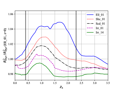
Figure 1: The change in $R_{\rm PSF}^{2}$ as a function of redshift for different galaxy types, normalised to an early type (Ell_01) spectrum at $z=0$. The six lines corresponds to the templates Irr_01, Irr_14, Ell_01, Scd_01, Sbc_01 and I99_05Gy from the CWW template library. The two vertical lines at z=0.4,1.3 indicate where the $\lambda=4000$Å break is entering and leaving the VIS filter.

Cropper et al. (2013) presented a detailed breakdown of the various systematic effects based on the expected performance of Euclid. It includes an allocation with the description ‘wavelength variation of PSF contribution’ in their Table 1, for which a contribution to the relative bias in effective PSF size of $|\delta R^{2}_{\rm PSF}/R^{2}_{\rm PSF}|=3.5\times 10^{-4}$ is listed. To include margin for additional uncertainties, we adopt here a slightly more stringent requirement of

$$\left|\frac{\delta R_{\rm PSF}^{2}}{R^{2}_{\rm PSF}}\right|\equiv\left|\left<\frac{R^{2}_{\text{Pred}}-R^{2}_{\rm PSF}}{R^{2}_{\text{PSF}}}\right>\right|<3\times 10^{-4},$$ (8)

where we explicitly average over an ensemble of galaxies ($\left<.\right>$). The predicted value of the effective PSF size, $R^{2}_{\text{Pred}}$, is the one we will attempt to estimate using supporting broad-band observations in multiple passbands, whereas the correct value is given by $R^{2}_{\text{PSF}}$. Note that this requirement is considerably tighter than what was studied in Cypriano et al. (2010).

This requirement is to be contrasted with the expected variation in effective PSF size for different galaxy types and redshifts. Figure 1 shows the relative change in $R^{2}_{\rm PSF}$ for five different galaxy SEDs as a function of redshift. Both the variation between galaxy types at a given redshift, and the variation with redshift for a given SED template are about two orders of magnitude larger than the requirement given by Eqn. 8. This figure highlights that incorrect estimates of the spectral type or photometric redshift can result in considerable biases in the adopted effective PSF. To explore this problem in detail we create simulated multi-wavelength catalogs, which we discuss next.

2.2 Simulated data

To quantify how well the effective PSF size can be determined from broad-band imaging data, we create simulated catalogs. In this paper we explore several approaches, which use observations of galaxies and stars. In our forecasts we consider the combination of Euclid observations in the VIS and NIR filters, with ground-based DES data. This is the baseline discussed in Laureijs et al. (2011) and also used in Cypriano et al. (2010). We use the extended CWW library (Coleman, Wu & Weedman, 1980) from LePHARE (Ilbert et al., 2006) which contains 66 SEDs. We split these into elliptical (Ell), spiral (Sp) and irregular (Irr) galaxies as described in Martí et al. (2014); they also describes how the SEDs are assigned. These galaxy realisations with absolute magnitudes, redshifts and SEDs are then converted into apparent photon fluxes ($f_{i}$):

$$f_{i} =\int d\lambda\,\lambda T_{i}(\lambda)S(\lambda(1+z))$$ (9)

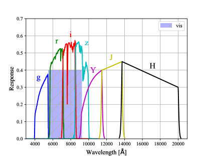
Figure 2: The Euclid (VIS, and near infrared Y,J,H bands) and DES (ground based g,r,i,z) effective filter response curves used to create simulate data. The effective filter response curves combine the atmospheric (for DES), telescope, filter and CCD transmission.

where $S(\lambda)$ is the rest-frame galaxy SED, $T_{i}(\lambda)$ is the response function in filter $i$ and the integration is over the observed frame wavelength. Figure 2 shows the adopted filter response functions ($T_{i}$) for the Euclid VIS and NIR filters, as well as the optical DES filters.

The simulated catalogs include realistic statistical uncertainties for the magnitudes. We assume that the measurements are limited by the noise from the sky background, which is independent between filters. Table 1 lists the adopted limiting magnitudes for DES and Euclid for point sources with a signal-to-noise ratio S/N=10. For galaxies, which are extended, we take a limit 0.7 magnitude brighter. We generate mock catalogs of galaxies that include galaxies that are fainter than $\text{VIS}<24.5$, but restrict the analysis to this limiting magnitude when estimating the relative bias in $R_{\rm PSF}^{2}$.

We explore various scenarios to estimate the effective PSF size, such as different combinations of broad-band imaging data. Of particular interest is the question whether it is possible to use the observed sizes and colours of stars to estimate the effective PSF sizes of galaxies: if a star and a galaxy would have the same SED, they would also have the same effective PSF. Figure 3 shows $R^{2}_{\rm PSF}$ as a function of colour for simulated galaxies and stars. The galaxies (yellow points) are a random subset of the simulated (noiseless) catalog, while the stars (black points) are generated by uniformly sampling all SEDs in the Pickles library (Pickles, 1998). For the filters that overlap in wavelength with the VIS band (panels with blue background) the relation between $R^{2}_{\rm PSF}$ and colour is indeed quite similar for galaxies and stars. The performance of this approach, extending the single colour estimate explored by Cypriano et al. (2010) to include the more extensive colour information, is explored in §4 using machine learning algorithms.

	VIS	$g$	$r$	$i$	$z$	$Y$	$J$	$H$
Galaxies	24.5	24.4	24.1	24.1	23.7	23.2	23.2	23.2
Stars	25.2	25.1	24.8	24.8	24.4	23.9	23.9	23.9

Table 1: The adopted limiting magnitudes for detections with a signal-to-noise ratio $S/N=10$. The limiting magnitudes for extended objects are assumed to be 0.7 magnitudes shallower than for point sources. The ground based observations (g,r,i,z) correspond to DES data, whereas the VIS, and Y,J,H correspond to the Euclid optical and NIR limits taken from Laureijs et al. (2011).

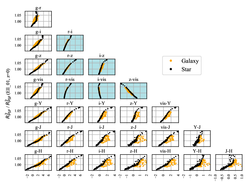
Figure 3: Relation between colour and the effective PSF size ($R^{2}_{\rm PSF}$) for different filter combinations (indicated in the title of each subplot). The black points show the results for stars with SEDs from the Pickles library (Pickles, 1998). The yellow points correspond to a random subset of galaxies covering a range of SEDs and redshifts. Subplots with a blue background indicate filters overlapping the VIS band.

3 Performance of template fitting methods

3.1 Photo-$z$ estimation

Cosmic shear studies rely on photometric redshifts (photo-$z$s) derived from deep broad-band imaging to relate the lensing signal to the underlying cosmological model. In this section we explore whether the algorithms used to determine photo-$z$s can also be used to estimate the size of the effective PSF.

These algorithms can broadly be divided into two classes. Machine learning methods train on a set of galaxies where the redshift is known from spectroscopy to predict the redshift for a larger ensemble of galaxies only observed using broad-band photometry. Examples of learning methods include the neural network algorithms ANNz (Collister & Lahav, 2004) and Skynet (Bonnett, 2015). Template based photo-$z$ methods (e.g. BPZ; Benítez, 2000; Coe et al., 2006) use libraries of the restframe galaxy SEDs. For each redshift and galaxy type, one can model the observed galaxy colours, and the best fit model is found by minimizing

$$\chi^{2}(z,\tau)=\sum_{i}\left[\frac{{\left(\tilde{f}_{i}-f_{i}(z,\tau)\right)}^{2}}{\sigma_{\tilde{f}_{i}}^{2}}\right]+\ \chi^{2}_{\text{Priors}(z,\tau)},$$ (10)

after marginalizing (summing) over the galaxy types ($\tau$). Here $\tilde{f_{i}}$ and $f_{i}(z,\tau)$ are the observed and predicted fluxes in the $i$th filter, with $z$ and $\tau$ being the galaxy redshift and template, respectively. The uncertainty in the flux is assumed to be Gaussian with a standard deviation $\sigma_{\tilde{f}_{i}}$. An optional prior term $\chi^{2}_{\text{Priors}}(z,\tau)$ adjusts the probabilities based on galaxy redshift and type, to reflect additional constraints, for instance the fact that bright galaxies are more likely to be at low redshift. This term reduces the number of degenerate solutions and catastrophic photo-$z$ outliers. In this paper we use the default BPZ priors specified in Benítez (2000). The template library is based on the same set of templates used to create the simulations.

Unlike learning methods, template based photo-$z$ methods also provide an estimate of the galaxy SED. From the best fit galaxy restframe SED ($S_{\rm best}(\lambda)$) and photometric redshift ($z_{\rm best}$), one can estimate the effective PSF size

$$R^{2}_{\tau,{\rm best}}=\frac{\int d\lambda\lambda T(\lambda)S_{\rm best}(\lambda(1+z_{\rm best}))R^{2}_{\text{PSF}}(\lambda)}{\int d\lambda\lambda T(\lambda)S_{\rm best}\left(\lambda(1+z_{\rm best})\right)},$$ (11)

where the integration is over the observed-frame wavelength. However, because of measurement uncertainties in the photometry, the template based codes not only provide the best fit redshift for each galaxy, but also a redshift probability distribution

$$p(z)\propto\exp{\left(-\frac{1}{2}\sum_{\tau}\chi^{2}(z,\tau)\right)},$$ (12)

where $\chi^{2}$ is given by Eq.10. Instead of using the best fit redshift (Eq. 11), one can instead estimate a PSF size, weighted by the redshift probability distribution:

$$R^{2}_{\tau,p(z)}=\frac{\int dzp(z)\int d\lambda\lambda T(\lambda)S_{\rm best}\left(\lambda(1+z)\right)R^{2}_{\text{PSF}}(\lambda)}{\int dzp(z)\int d\lambda\lambda T(\lambda)S_{\rm best}\left(\lambda(1+z)\right)}.$$ (13)

This can be extended further by also including the probabilities of the galaxy types. We compare the performance of these choices for the effective PSF size estimates in §3.3.

The template library uses the following six templates: Ell_01, Sbc_01, Scd_01, Irr_01, Irr_14, I99_05Gy, which represent a subset of the SEDs in the galaxy mocks. This limited set of SEDs reflects the conventional use of photo-$z$ algorithms and the fact that the real SEDs are not perfectly known. We explore this in more detail in §3.4, but note that the photo-$z$ code does include two linear interpolation steps between consecutive templates to mimic a smooth transition between templates. When determining photometric redshifts from the mock galaxy catalogs we exclude the VIS band, since it only yields a minor improvement in the photo-$z$ precision, while it would increase the covariance between the photometric redshift and the shape measurements.

3.2 Simple scenario

The photo-$z$ algorithm provides an estimate of the restframe SED, while the calculation of the effective PSF size is done using the galaxy SED in the observed frame. The conversion between the two frames requires the redshift, which causes the redshift biases and uncertainties to directly affect the estimate of $R^{2}_{\rm PSF}$ from a template based photo-$z$ code. The photo-$z$ probability density distribution that is provided by a template fitting algorithm can be a complex function of redshift, as degenerate solutions may be found with different best-fit SEDs. Before examining this complex, but more realistic situation, we consider a number of simpler cases that allow us to disentangle the different effects.

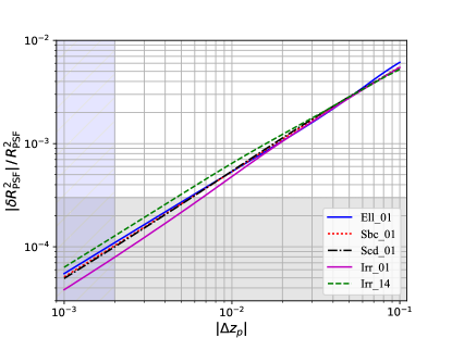
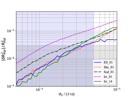
Figure 4: Effect of Gaussian photo-$z$ uncertainties on the estimate of $R^{2}_{\rm PSF}$ for a known rest-frame SED. The lines show the relative bias $\delta R^{2}_{\rm PSF}/R^{2}_{\rm PSF}$ for different galaxy templates at $z=0.5$. In the top panel the photo-$z$ bias varies (no photo-$z$ scatter), while the bottom panel varies the photo-$z$ scatter (no photo-$z$ bias). The solid (gray) shaded region shows the required accuracy. In the top panel the hatched (blue) region indicates a photo-$z$ bias $<0.002(1+z)$ within a redshift bin, while it marks a photo-$z$ scatter $<0.05(1+z)$ in the bottom panel.

The top panel in Fig. 4 shows the absolute value of the relative bias in effective PSF size if we assume that the SED is known a priori, but where the best-fit photo-$z$ is biased by $|\Delta z_{p}|$. While the size of the bias varies with redshift, we limit the discussion here to $z=0.5$ for simplicity, and use the full redshift range for the realistic simulations (see §3.3). The amplitude of the bias increases with increasing redshift bias, with the different templates yielding rather similar results. We find that if $|\Delta z_{p}|<0.005$ the resulting bias in PSF size is within the adopted allocation for Euclid (indicated by the grey shaded region). This may appear challenging, but a correct interpretation of the cosmic shear signal requires that the bias in the mean redshift for a given tomographic bin is known to better than $|\Delta z|<0.002(1+z)$ (Laureijs et al., 2011) and thus for an ensemble of galaxies the resulting bias in the PSF size may be sufficiently small. However, the redshift sampling of photometric redshift codes is typically $\Delta z\sim 0.01$, which may introduce biases. We examine this in detail in Appendix A and find this is not a concern.

The situation is more problematic when we consider the uncertainty in the photometric redshift estimate, which we assume to be a Gaussian with a dispersion $\sigma_{z}$ around the correct redshift (i.e. no bias). The bottom panel in Fig. 4 shows the relative bias in the effective PSF size as a function of $\sigma_{z}/(1+z)$ for galaxies at $z=0.5$, demonstrating that a small photo-$z$ scatter can cause a substantial bias in the estimate of the effective PSF size. The bias increases with increasing uncertainty, with the largest bias occurring for the Irr_01 template. The requirements for the cosmic shear tomography for Euclid are that $\sigma_{z}/(1+z)<0.05$ (Laureijs et al., 2011), and hence the resulting biases in PSF size are somewhat larger than can be tolerated. However, in reality one averages over a sample of galaxies within a tomographic bin, and thus these numbers should not be considered appropriate requirements. Nonetheless they indicate that the statistical uncertainties in the photometric redshifts are important.

3.3 Conventional template fitting method

After considering the simplistic case of galaxies with a known SED and Gaussian photo-$z$ errors, we now examine the performance of a template fitting method using the more realistic galaxy simulations described in §2.2. As a consequence, the results include redshift outliers and misestimates of the galaxy rest-frame SED.

Sample	All	Ell	Sp	Irr
Peak	7.2	14	2.4	-1.6
Pdf(z)	-0.3	12	-8.9	-18
Pdf(z,sed)	4.1	13	-2.1	-11

Table 2: The mean relative bias in effective PSF size times $10^{-4}$ when using a photo-$z$ template fitting method. Columns show the results by galaxy type: Elliptical (Ell), Spiral (Sp) or Irregular (Irr) galaxies. The rows list the relative bias when using the best fit photo-$z$ (Peak) and when weighting using the redshift pdf (PDF).

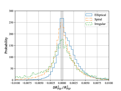
Figure 5: The distribution of relative biases $\delta R^{2}_{\rm PSF}/R^{2}_{\rm PSF}$ for different galaxy types using a photometric redshift template fitting code. The galaxies are split into Elliptical, Spiral and Irregular types based on the definition in the input mock catalogue. The vertical band marks the Euclid requirement for the mean relative bias.

As mentioned earlier, the template fitting algorithm provides an estimate for the best fit redshift and rest-frame SED, but also a probability density distribution for the redshift (which may be combined with a distribution of templates $\tau$). The different outputs can be used to estimate the average bias in the effective PSF size. Table 3.3 lists the resulting average values for $\delta R^{2}_{\rm PSF}/R^{2}_{\rm PSF}$ when splitting by the true galaxy types. If we consider the best fit redshift estimate, the biases are small for both the spiral and irregular galaxies, whereas the biases are large for early type galaxies, irrespective of the weighting scheme.

It is also instructive to examine the distribution of biases for the different galaxy types. Figure 5 shows that the distribution of effective PSF sizes is much broader than the requirement. For all three galaxy types the distribution peaks close to zero, and the bias for all three types is caused by the skewness towards larger $R_{\rm PSF}^{2}$ values, because the redshift errors and SED misestimates do not fully cancel.

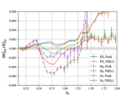
Figure 6: Redshift dependence of the relative bias in the effective PSF size when a photo-$z$ template fitting method is used. The plot shows results split by input galaxy type and for two approaches to determine $R^{2}_{\rm PSF}$, i.e. using the best fit photometric redshift, or using the full $p(z)$. In both cases we do not marginalize over the uncertainty in the SED. The horizonal band marks the Euclid requirement.

The results in Table 3.3 are averages over the full redshift range, but the broad distributions in Fig. 5 for the three galaxy types suggest that other parameters play a role. Figure 6 shows the relative bias in $R^{2}_{\rm PSF}$ for different estimators as a function of redshift. Note that the number of irregular galaxies in our simulations is negligible at $z>1.5$, because they are fainter than our magnitude cut, and the measurements therefore only extend to this redshift. The variation as a function of redshift is the main cause of the broad distributions in Fig.  5, and is much larger than can be tolerated. This demonstrates that a simple average over the full galaxy sample is not adequate. In general using the best-fit redshift and the redshift weighting yields very similar results, although the averages differ somewhat. We therefore focus on the results using the best-fit redshift below.

3.4 Restricted template fitting

It is interesting to investigate which parameters of the experimental setup affect the bias in effective PSF size the most, as they may provide clues how to improve the performance. We therefore examine a range of scenarios where we modify the set of filters used, examine the SED coverage of the algorithm, as well as the role of the photo-$z$ priors.

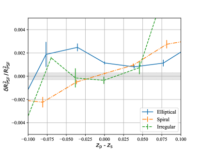
Figure 7: Effect of a redshift error on the estimate for $R_{\rm PSF}^{2}$. The plot shows the relative bias $\delta R^{2}_{\rm PSF}/R^{2}_{\rm PSF}$ when using a photo-$z$ template fitting method for three input galaxy types as a function of the difference between estimated and true redshift. The horizonal band marks the Euclid requirement.

The observed frame SED in the VIS filter is the most important quantity when estimating the effective PSF size because the shapes are measured using these images. In §3.2 we already saw that the errors in the photometric redshifts can introduce bias. As we kept the SED fixed in this case, we effectively modified the observed SED. One might naively assume that the algorithm will adjust the best fit SED accordingly, thus reducing the bias. To quantify this, we show the relative bias in effective PSF size as a function of the difference between the best-fit photo-$z$ $z_{p}$ and the true redshift $z_{s}$ in Fig. 7. In this case the algorithm is free to adjust the SED. For the late type SEDs the results look qualitively similar to what was found in §3.2, but for the early type galaxies the effective PSF size is overestimated consistently. Hence it is incorrect to assume that errors in the photo-$z$ estimate are compensated by selecting a different SED. We find that only using r,i,z data does not reduce the bias.

In template based photo-$z$ methods the flux measurements in the various filters are compared to the model, and additional priors are used to restrict the range of solutions. The former can be split further into the contributions that arise from the r,i,z filters that overlap with the VIS band, and the out-of-band filters ($\textit{g},\textit{Y},\textit{J},\textit{H}$ in our case). Minimising $\chi^{2}$ using the contributions from the out-of-band filters and the photo-$z$ priors only provides indirect information on the SED in the VIS band and may thus lead to biases in the estimate for the PSF size. It is therefore of interest to examine whether the performance improves by restricting the filters used. Reducing the statistical uncertainties in the flux measurements may provide another way to improve the performance.

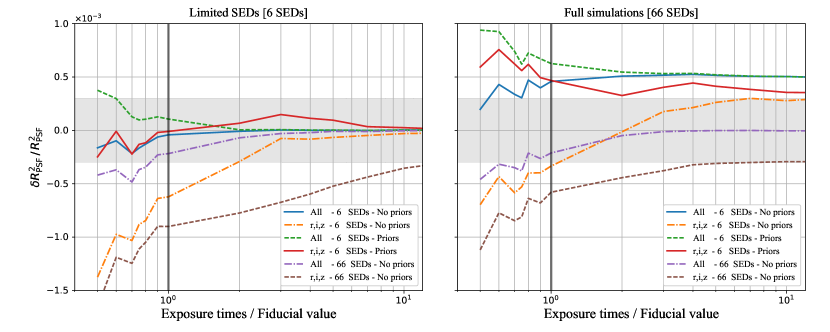
Figure 8: $\delta R^{2}_{\rm PSF}/R^{2}_{\rm PSF}$ for the SED template fitting method. On the x-axis the exposure time is scaled relative to the fiducial setup. In the left panel the simulated galaxy catalog only include the 6 templates used in the photo-$z$ code, while for the right panel it includes the full 66 templates. The lines show which combination of filters was used (All or $r,i,z$), whether priors were used (No priors or Priors), and how many SEDs were used. The vertical line indicates the fiducial setup, while the shaded (gray) band marks the Euclid requirement.

Figure 8 shows the relative bias for the full sample as a function of exposure time (relative to the nominal case), where we assumed that the increase in exposure time is the same for all filters, including the Euclid VIS and NIR filters. We do so for different setups. In the left panel we create simulated catalogs using only six distinct SEDs, whereas in the right panel the full range of SEDs is used. We do keep the luminosity functions for the various galaxy types unchanged, but rather assign slightly different SEDs to each type.

For the simulations with six SEDs (left panel) there are several combinations of filters that meet the requirement on the average relative bias (as indicated by the grey region). If the filter set is restricted to r,i,z, the priors are needed to reduce the average bias for the fiducial exposure time, but otherwise applying the photo-$z$ code with only six templates performs well. As expected, in the noiseless limit the bias vanishes for all setups with six templates. While the galaxy priors and the g,Y,J,H only contribute indirectly to constrain the SED within the VIS band, including these does reduce the bias in the PSF size.

Of particular interest are the two cases where the photo-$z$ algorithm uses all 66 templates in the analysis: the biases are larger, although they do vanish in the noiseless case (with the r,i,z scenario converging outside the plot). The larger bias can be understood, because the noise causes the algorithm to select SEDs not in the simulations. While adding more templates in the fitting code may be tempting, this result cautions us that it can also lead to biases.

The right panel in Fig. 8 shows the results when the full range of SEDs is used to create the simulated catalogs. In this case we find that using only six templates in the photo-$z$ algorithm leads to biases, even in the noiseless case. The r,i,z setup without photo-$z$ priors accidentally meets the requirements for the nominal exposure time. Using the full range of SEDs in the analysis improves the performance, as expected, with the best results for the case where all filters are used. These results highlight the need for the photo-$z$ templates to span the full set of SEDs in the observations, which may be challenging in practice.

4 Machine learning techniques

The results presented in the previous section suggest that modifications to the template fitting codes are needed if these are to be used to determine the effective PSF. Motivated by the fact that Fig. 3 shows that the PSF sizes for galaxies correlate strongly with the observed colour, we explore the use of machine learning methods as a possible alternative to map between the observed colours and the effective PSF.

Although machine learning techniques are fast, flexible and easy to implement, the spatial variation of the PSF introduces additional complications which may be less straightforward to implement; in contrast the effective PSF is readily computed given a model for the PSF and the SED from a template fitting code. Regardless of which approach may be best suited for the analysis of Euclid data, quantifying the performance of the machine-learning methods allows us to assess whether the supporting ground-based observations for Euclid are adequate to infer the effective PSF.

4.1 Training on simulated galaxy photometry

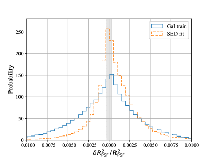
Figure 9: Histogram of $\delta R^{2}_{\rm PSF}/R^{2}_{\rm PSF}$ values when using a template fitting photo-$z$ code (dashed green) and when training on r,i,z data from a simulated galaxy catalog (blue).

To explore the performance of machine learning we create a training sample of galaxy simulations using the same procedure as the test catalog (as described in §2.2). We start with a best case scenario where the training set does not contain noise. The NuSVR algorithm from scikit-learn (Pedregosa et al., 2012) is used to train on a sample of 4000 galaxies with multi-wavelength measurements. The galaxy training and test catalogs are generated with the same algorithm, but they are separate realisations.

The results are used to estimate the effective PSF sizes of the test catalog (which does contain noise). A histogram of the residuals when we train on 4000 galaxies with r,i,z photometry is presented in Fig. 9 (solid histogram). The distribution of residuals is fairly symmetric and centred around zero bias: we observe an average value of $\delta R_{\rm PSF}^{2}/R_{\rm PSF}^{2}=3.5\times 10^{4}$ (also see Table 3). For comparison we also show (dashed histogram) the residuals from the template fitting method (all filters, priors, photo-$z$ peak). The residuals from the SED fitting method also peak around zero, but the distribution is noticeably skewed, which leads to a significant bias when averaged over the full sample.

We also consider a number of scenarios where different filter combinations are used to train. The resulting average biases are listed in Table 3. The results in the second column are for noiseless photometry, whereas noisy data were used in the training for the results listed in the third column. We find that all configurations perform well, with the exception of the case where only $i,z$ data are used to train. This can be understood from Fig. 3, which shows that for all colours the colour-$R^{2}_{\rm PSF}$ relation is tightest for colours that include the r-band. Interestingly, we find that the combination of $r,i$ performs better than the r,i,z setup. This is because the VIS filter covers only the blue half of the $z$-band. Hence the information contained in the $z$-band measurements is of limited value as some of the flux falls outside the VIS filter. We verified this with a test where the $z$-band was restricted to the blue half: the bias was reduced, whereas the bias increased when we used the redder half.

Although perhaps somewhat counterintuitive, we advocate to exclude the $z$-band when a restricted set of filters is used to estimate the effective PSF when training using galaxy templates. We explore this setup in more detail in Appendix C. Including more filters does reduce the bias, but it is not clear whether this would work in practice because of variations in photometric calibration. Especially including the NIR data would lead to additional requirements on the relative calibration between the ground-based optical data and the Euclid NIR data.

Filters	Gal	Gal-noisy	Star	Star-noisy
r,i,z	1.2	3.0	2.1	2.8
r,i	0.4	1.0	9.7	12
i,z	11	13	40	38
vis,r,i,z	1.4	1.8	1.2	2.0
vis,r,i	2.0	0.2	7.4	8.5
vis,i,z	1.3	7.7	27	26
All	0.1	1.7	9.9	8.3
All - vis	0.1	1.8	1.7	2.5
All - r	0.4	4.7	1.8	1.8
All - z	0.1	1.0	6.1	4.7
All - vis,z	0.1	1.8	4.4	3.7

Table 3: The absolute value times $10^{4}$ of the relative bias $|\delta R^{2}_{\rm PSF}|/R_{\rm PSF}^{2}$ when using a machine learning method for different instrumental setups and training approaches. The first two columns (Gal) list results when the algorithm is trained on galaxy simulations, while the last two columns (Star) correspond to the biases when the algorithm is trained on stars. The columns marked ‘-noisy’ include noise and the others are noiseless. The first column lists the filters used. Here ’All’ means g,r,i,z,VIS,Y,J,H. and ‘All - filter’ means that the filter was omitted.

4.2 Training on observed photometry of stars

So far, our attempts to predict the effective PSF size have focused on galaxy templates. The predicted SED is then used with a model of the wavelength dependence of the PSF to compute the value for $R_{\rm PSF}^{2}$. On the other hand, the PSF properties, including higher order moments of the surface brightness distribution, can be measured directly for stars in the data. Moreover, Fig. 3 shows that galaxies and stars with the same colour have very similar effective PSF sizes. It is therefore interesting to examine whether it is possible to train on a sample of stars instead.

The main benefit of such an approach is the potential of constructing a self-calibrating method: when training on, and applying the results to the same pointing, this implementation would be rather insensitive to calibration errors in the photometric zero-points. The effective PSF can be computed using the wavelength-dependent model of the PSF and the SEDs of the stars. The resulting mapping between effective PSF parameters and observed star colours could then also be applied using the observed colours of galaxies. As before, we focus on the effective PSF size for simplicity.

We start with noise-free measurements of the colours of stars. For the star catalogs we use 400 stars, uniformly sampled from stellar SEDs in the Pickles (Pickles, 1998) library. A typical Euclid pointing is expected to contain more stars, and thus these results give a conservative indication whether self-calibration is feasible. On the other hand, the distribution of stellar SEDs is wider than in actual data. We explore this further in §4.3 where we use a realistic distribution of spectral types from the second data release of the KiloDegree Survey (KiDS; Kuijken et al., 2015).

To mimic a self-calibration procedure, we create 100 independent pointings, and train the NuSVR algorithm on the star simulations. The last two columns in Table 3 list the results when we train using the star catalogs. The biases are generally small, and in some (noise-free) cases this approach outperforms the training on galaxy templates. This the consequence of the fact that the stars show a remarkably simple relation between the colour and $R_{\rm PSF}^{2}$ (see Fig. 3). An important difference is the increase in bias when excluding the z-band, which did not occur when training with galaxies. Including the VIS band reduces the bias, albeit with limited effect. As was the case for the galaxies, including VIS and NIR data can help, provided the relative calibrations between the various data sets can be ensured.

4.3 Tomography and calibration sample

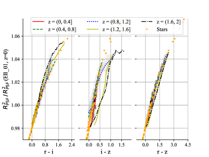
Figure 10: Effective PSF size $R^{2}_{\rm PSF}$, relative to the value for the Ell_01 SED at $z=0$, versus colour for filters that overlap with VIS. Stars are marked as dots, while galaxies are binned in redshift ranges and shown as lines. The hex-bins shows the density for the full galaxy population. No magnitude noise is included.

The constraints on cosmological parameters from cosmic shear surveys are improved significantly if the source sample is split in a number of narrow redshift bins, such that they are sensitive to the matter distribution at different redshifts. Such ‘tomographic’ analyses are now standard for cosmic shear studies (e.g. Heymans et al., 2013; Becker et al., 2016; Jee et al., 2016; Hildebrandt et al., 2017), and therefore it is not sufficient to consider the bias for the full sample, especially because the effective PSF size varies strongly with redshift. Hence, even though training on stars results in an overall small bias in the effective PSF size, we need to ensure that the bias does not vary significantly with redshift. We already saw that this was problematic for template fitting methods (see Fig. 6).

Figure 10 shows the relative change in $R^{2}_{\rm PSF}$ for galaxies and stars as a function of the colours that overlap the VIS-band. Similar to what we saw in Fig. 3, the stars (orange points) trace the overall galaxy population well (grey hexagons), but when we split the galaxy sample into redshift bins (indicated by the lines), we find that this good correspondance does not hold for all redshifts: especially for the highest redshifts the relation is very different, which is problematic for a machine learning method. This result is similar to the conclusion reached by Cypriano et al. (2010) who considered only a single colour.

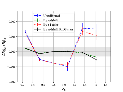
Figure 11: The relative bias in effective PSF size for different calibration methods, when 400 stars that are uniformly sampled from the Pickles SED library (Pickles, 1998) are used for the training step. The dashed-dotted blue line shows the results without further calibration, showing a strong redshift dependence. The dotted red line indicates the results when the bias is adjusted based on the r-i colour. The dashed green line shows that the bias can be reduced significantly when an redshift-dependent offset in the r magnitude is applied. The solid black line uses a stellar SED distribution from fitting to KiDS data (see text). The errors are estimated from 100 pointings and the horizontal band marks the required accuracy.

To examine this in more detail, we train on a star catalog using the r,i,z bands (see §4.2) and compute the residual bias in the effective PSF size as a function of redshift. The results are presented in Fig. 11 by the blue dashed line, and show a clear redshift dependence. The bias is higher at both low and high redshifts, but these redshift ranges contain fewer galaxies. When averaging over redshift the biases largely cancel, leading to a low average value for the full sample. Such a redshift dependent bias is problematic as it may mimic an interesting cosmological signal, and our results demonstrate that it is not sufficient to specify a requirement for the full sample.

We explored various approaches to model the redshift-dependent bias, but were unable to do so directly. Instead we opted for a hybrid approach using a simulated galaxy catalog as a ‘calibration’ sample. We train on the stars as before, but use the simulated galaxy catalog to adjust the method to create an unbiased estimate of the effective PSF size. Although such an implementation is no longer fully self-calibrating, training on the observed stars may still valuable, if it can reduce the sensitivity to errors in the photometric calibration and the wavelength dependence of the PSF model, as well as the adopted library of galaxy templates (see §5 for more details). On the other hand, the performance may still be limited by the fidelity of the calibration sample that is used.

One possibility is to adjust the bias in effective PSF size by accounting for the difference in size as a function of $r-i$ colour between stars and galaxies, as is indicated in Fig. 10. The dotted red line in Fig. 11 demonstrates, however, that this does not alleviate the strong redshift dependence. Instead, as is explained in more detail in Appendix B, we found that it is possible to reduce the bias effectively by introducing an r-band offset that depends on redshift, without increasing the scatter significantly. However, in practice photometric redshifts are used, and we examine the consequences of this in the next subsection.

The adopted redshift-resolution for this correction allows us to adjust the importance of the galaxy templates on the results: if we assume no redshift dependence the method reverts back to training on stars, whereas a very fine redshift sampling is identical to training on galaxy templates. As discussed in Appendix B we adopted a redshift sampling of $\Delta z=0.18$, which appeared to be a reasonable compromise between the two extremes. In §5.1 we compare the performance of the hybrid approach to the training on galaxy templates in the presence of calibration errors in the photometric data.

The distribution of stellar SEDs is expected to vary, in particular as a function of Galactic coordinates. To explore the impact of such variations we determine the SED distribution by fitting the Pickles library to the g, r, i, z for stars ($i_{AB}<21$, $\text{CLASS\_GAL}>0.8$) in KiDS DR2. For each Euclid pointing we simulate 400 stars generated using the stellar distribution in a KiDS pointing limited to the 15 most frequent templates. We find that the bias is essentially unchanged compared to the case of training on a uniform distribution of templates.

4.4 Correlations between photometric redshift and effective PSF size

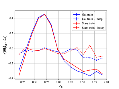
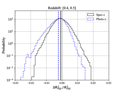
Figure 12: Top: Pearson correlation coefficient between the residual bias in the effective PSF size, $\delta R_{\rm PSF}^{2}/R_{\rm PSF}^{2}$ and photo-$z$ error, $\delta z$, as a function of true redshift. The effective PSF size was estimated using the r,i,z bands only, whereas the photometric redshifts use measurements from all available filters. The blue lines show the results when galaxy mocks are used for the training, whereas the red lines show the results when stars are used (but no additional calibration applied). The solid lines indicate the results for the realistic case when the same r,i,z data are used to measure both PSF size and photometric redshift (i.e., the noise is in common), whereas the dashed lines are for independent realisations of the data. The error bars are estimated from simulating 100 pointings. Bottom: Histogram of $\delta R_{\rm PSF}^{2}/R_{\rm PSF}^{2}$ for the redshift range [0.4, 0.5] when selecting either on spec-z (solid black) or photo-$z$ (dashed blue). The training uses stars in the r,i,z bands and the histograms comprise 100 independent pointings.

The results presented in Fig. 11 show that the biases as a function of true redshift can be reduced to the required level. However, in practice, tomographic bins are based on the photometric redshifts. The large uncertainties and potential outliers may affect the performance of the approach outlined above. Moreover, as the photometric redshift estimate and the determination of the effective PSF make use of the same data (at least in part), correlations may be introduced. We explore these more practical complications here.

To quantify the correlation between the relative error in the inferred effective PSF size $\delta R_{\rm PSF}^{2}/R_{\rm PSF}^{2}$ and the error in the best fit photometric redshift $\delta z\equiv(z_{\rm b}-z_{\rm true})/(1+z_{\rm true})$ we define the Pearson correlation coefficient

$$r(\delta R_{\rm PSF}^{2},\delta z)\equiv\frac{\left<\delta R_{\rm PSF}^{2},\delta z\right>}{\sqrt{\text{Var}(\delta R_{\rm PSF}^{2})\text{Var}(\delta z)}}$$ (14)

where $\text{Var}(.)$ is the variance. The solid lines in Fig. 12 show the correlation coefficient between the error in the effective PSF size and $\delta z$ as a function of true redshift when training on galaxies or stars, respectively. In both cases we find a significant positive correlation between the errors between $0.4<z<1$ and an anti-correlation at high redshifts. In contrast, the dashed lines show the results when the effective PSF size and photometric redshift determinations are obtained using independent data sets, i.e. independent noise realisations. In this case the correlation coefficient is close to zero for both training cases.

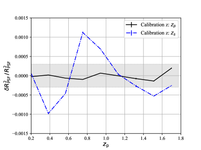
Figure 13: $\delta R_{\rm PSF}^{2}/R_{\rm PSF}^{2}$ as a function of photometric redshift, using either the photometric redshift or the true redshift in the calibration catalog. The training uses observations of stars in the r,i,z bands and the uncertainties are estimated from 100 pointings.

These results demonstrate that the (re-)use of photometric data for different measurements may lead to redshift dependent correlations between residuals. To examine this in more detail we consider a single redshift bin with $0.4<z<0.5$, where the selection can be done either based on spectroscopic or photometric redshift. The resulting distributions of the relative bias in effective PSF size are presented in the bottom panel of Fig. 12. When the galaxies are selected by spectroscopic redshift the distribution is symmetric, and the mean bias meets our requirement. However, selecting galaxies based on their photometric redshift leads to a skewed distribution with a significant bias in the mean. This is the result of the correlation between $\delta z$ and $\delta R_{\rm PSF}^{2}/R_{\rm PSF}^{2}$: a selection in photometric redshift leads to a selection in effective PSF size. Hence an unbiased estimate for tomographic bins needs to account for this correlation.

This is achieved naturally when correcting the bias in effective PSF size using the simulated galaxy catalog: the redshift dependence of the applied offset in $r$ magnitude can be determined by splitting the galaxies as a function of photometric redshift. As shown by the solid black line in Fig. 13, this removes the impact of the correlation between the $\delta z$ and $\delta R_{\rm PSF}^{2}/R_{\rm PSF}^{2}$, since this is also included in the calibration sample. In contrast, when the calibration sample is instead split based on the true redshift, $z_{s}$, the bias exceeds requirements (blue dashed line). These results indicate that the calibration step can reduce the bias when using photometric redshifts, provided that the simulations are sufficiently accurate. We note, however, that the training needs be done after the tomographic bins have been defined.

5 Calibration

5.1 Impact of calibration errors.

So far we have assumed that the flux measurements in the various bands used to infer the effective PSF size are perfectly calibrated and that the wavelength dependence of the PSF is known. In practice the zeropoints in the r,i,z bands will vary across the survey, although we note that (some) modern surveys can achieve impressive homogeneity (e.g. Finkbeiner et al., 2016). Moreover, the wavelength dependence of the PSF is expected to be well-known, but it will vary with time due to variations in the optical system.

A machine-learning algorithm trained on the observed stars establishes the mapping between the observed colours and PSF size, rendering it insensitive to zero-point offsets and errors in the PSF model. Interestingly, problems with the photometry and PSF model could be identified by examining the observed sizes to the ones expected based on their SED. For instance, the colour-$R^{2}_{\rm PSF}$ relation is shifted by a magnitude offset and can thus be used to detect biases in the ground based photometry. Deviations from the expected wavelength dependence of the PSF can be directly tested by comparing the observed PSF to the wavelength dependent PSF model, $R^{2}_{\rm PSF}(\lambda)$, convolved with stellar spectra.

Unfortunately we found in the previous section that it was not possible to estimate the effective PSF using the stars alone, because it resulted in strong redshift dependent biases. We therefore need to quantify the impact of calibration errors on the estimate of the effective PSF size. We compare the sensitivity of the two machine-learning implementations discussed in the previous section. Although both approaches ultimately rely on simulated galaxies, the hybrid method may retain some of the advantages of self-calibration, and thus the sensitivity to calibration errors may still be reduced. In this subsection we use the r,i,z observations of stars to train the algorithm, although we note that the results are qualitatively the same when only $r,i$ data are used, albeit with a somewhat larger scatter in the latter case.

Figure 14: The allowed range in offset in the power law slope of the PSF size as a function of wavelength, $\gamma$, such that the bias in effective PSF size does not exceed the Euclid requirement. The black bars indicate the results for the hybrid approach, and the blue bars when we train using galaxy SEDs. To obtain these results we applied the offset to the simulated galaxy and star data, while the galaxy training and calibration sample use the nominal value of $\gamma=0.55$. This corresponds to an unknown $\gamma$ shift in the data. On the y-axis we show the requirement for the full sample (all) and when splitting in redshift bins. The five redshift bins are: [0.10, 0.44), [0.44, 0.78), [0.78, 1.12), [1.12, 1.46) and [1.46, 1.80), in increasing order.

We first examine the sensitivity to the wavelength of the PSF, which we assume to be a power law $R_{\rm PSF}^{2}\propto\lambda^{\gamma}$, where $\gamma=0.55$ is the nominal value used so far. We assume that an error in the PSF model is captured by a change in the value of $\gamma$. For the full sample and different redshift bins, we find that the relative bias in effective PSF is a linear function of $\delta\gamma$, the change in the power law slope. We use these relations to determine the maximum change $\delta\gamma$ that can be tolerated such that the bias in effective PSF size is smaller than the Euclid requirement. The results are shown in Fig. 14 for both training approaches. Note that this shift is applied to the simulated observations, but that the calibration sample is not changed.

We find that the lowest redshift bin is remarkably insensitive to changes in the PSF model, and that the requirements are rather similar for the two training approaches. We do note that the galaxy-only case for the fourth redshift bin represents a challenge: as the sign of $\delta\gamma$ is in principle unknown, we obtain $|\delta\gamma/0.55|<2.4\times 10^{-3}$. When we consider the hybrid method that trains on stars first, we find that $|\delta\gamma/0.55|<5\times 10^{-3}$ is needed to meet the requirement on the relative bias in effective PSF size. Although this may appear challenging, such a deviation represents noticeable deviation in the optical model of the PSF. Moreover, the Euclid PSF is expected to be very stable in time, and thus changes in $\gamma$ can be easily monitored.

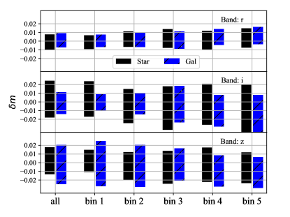
Figure 15: The allowed range in magnitude offsets that can be tolerated for Euclid. The black bars indicate the results for the hybrid method, and the blue bars when training on galaxies only. In both cases only r,i,z data were used to train on. In the top, middle and bottom panels, the offsets are applied to the r,i and z-band independently. On the y-axis we show the requirement for the full sample (all) and when splitting in redshift bins. The five redshift bins are: [0.10, 0.44), [0.44, 0.78), [0.78, 1.12), [1.12, 1.46) and [1.46, 1.80), in increasing order.

We now proceed to examine the sensitivity to errors in the calibration of the ground-based observations, which may occur because of varying observing conditions. Repeated observations of the same field allow for exquisite homogeneity (Finkbeiner et al., 2016). In the near future, however, Gaia (Perryman et al., 2001) spectrophotometric measurements should provide an excellent reference across the full sky in this wavelength range. Nonetheless it is important to evaluate what errors in photometric zeropoint can be tolerated.

To examine this we apply an offset to the simulated observations in each of the optical bands used and calculate the relative changes in the effective PSF size. To do so, we change the zeropoint in one filter while keeping the other measurements unchanged, and determine the maximum shifts in zeropoint that are still within requirements and show the results in Figure 15 for the full sample of galaxies and the five tomographic bins in true redshift. The results show that the effective PSF is most sensitive to photometric calibration errors in the $r$ band: for the hybrid method we find that $|\delta m|<0.005$ in the $r$-band, whereas $|\delta m|<0.01$ appears adequate for the other filters. Such a level of photometric homogeneity seems quite achievable. Training on galaxy simulations alone would increase the sensitivity to magnitude offsets in the r-band such that $|\delta m|<0.003$. Hence the hybrid method of training on stars, followed by a redshift dependent adjustment determined using simulated galaxies retains some of the self-calibration properties.

5.2 Sensitivity to template library

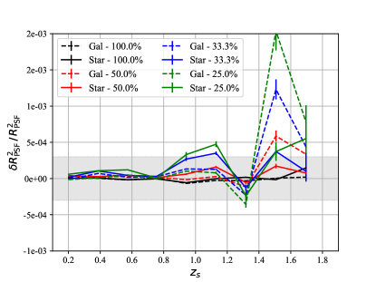
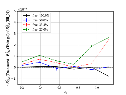
Figure 16: Top: The relative $R^{2}_{\rm PSF}$ bias when limiting the SEDs in the galaxy training and the calibration sample. Solid and dashed lines show $\delta R^{2}_{\rm PSF}\,/\,R^{2}_{\rm PSF}$ when training on stars and galaxies, respectively. The template removal is done uniformly over the 66 SEDs and legend shows the fraction remaining. On the x-axis it the spectroscopic redshift. Bottom: The mean difference between the $R^{2}_{\rm PSF}$ predicted when training on simulated observed stars and simulated galaxies. The errorbars for both panels are estimated from 100 Euclid pointings.

Given that both machine-learning approaches rely on a library of simulated galaxy SEDs, a key remaining question is whether the results are sensitive to limitations of the template library. In §3.4 we already saw that the performance of the template fitting code depends on the number of templates used, especially if the number was too low. We therefore return to this issue here and examine the impact of an incomplete SED library on the machine-learning approaches.

The top panel in Fig. 16 shows $\delta R^{2}_{\rm PSF}\,/\,R^{2}_{\rm PSF}$ when we limit the SED coverage in the galaxy training sample and the calibration sample used to adjust the predictions when training on stars first. The legend shows the fraction of SEDs which remain after uniformly removing templates from the simulations. For a complete sample ($100\%$), the bias in effective PSF size is small for both approaches. When omitting galaxy templates, the hybrid method performs better at high redshift. Overall, both methods appear fairly robust to an incomplete template library, although this may need to explored further; especially the impact of emission-line galaxies and dusty galaxies has not been explored.

As the hybrid method requires the same template library, one may be tempted to omit this approach. Regardless, we need to somehow ensure that the template library is adequate. This can be done by comparing the results from the two methods, as their dependencies on the template library is different. This is evident from the top panel in Fig. 16. The bottom panel of Fig. 16 shows the difference in the estimate of the effective PSF size, relative to that of an early type galaxy, as a function of redshift. If the template library is highly incomplete, the two PSF estimates differ significantly, especially for high redshift galaxies. This can thus be used as a way to validate the machine-learning approach.

6 Conclusion

The convolution of galaxy images by the PSF is the dominant source of bias for weak gravitational lensing studies, and an accurate estimate of the PSF is thus essential for a successful measurement. In this paper we studied the bias caused by the combination of a wavelength dependent PSF and limited information about the SED of a galaxy of which we wish to measure the shape. We quantified the impact on the performance of Euclid, for which the impact is exacerbated because of the combination of a (near-)diffraction limited PSF and the broad VIS pass-band. We note, however, that the wavelength dependence of the PSF cannot be ignored for other stage IV ground-based surveys such as LSST.

Based on the analysis of biases by Massey et al. (2013), we restricted the study to the determination of the effective (or SED-weighted) PSF size, which is different for each galaxy. Under the assumption that an accurate model of the PSF as a function of wavelength can be derived, we explored several approaches to estimate the effective PSF size from a number of broad-band images. Given the exquisite precision with which Euclid can measure the cosmic shear signal, the corresponding accuracy with which the PSF properties need to be determined makes this challenging. Following Cropper et al. (2013) we consider a maximum relative error of $3\times 10^{-4}$, whereas the variation in effective PSF size with source redshift is two orders of magnitude larger (see Figure 1).

We simulated catalogs of stars and galaxies based on the expected depth and wavelength coverage of DES and Euclid. We used these to examine how well a standard template fitting photo-$z$ code can predict the effective PSF for a galaxy. We found that the resulting distribution of predicted PSF sizes is skewed, leading on biases in the estimate of the effective PSF that exceed the requirements. Hence, modifications to the template fitting codes are needed if these are to be used for this purpose. We note that this may be worthwhile, because the effective PSF can be computed using a multi-wavelength model of the spatially varying PSF and the SED from a template fitting code.

To quantify the expected performance for different scenarios of multi-wavelength data, we used machine-learning methods instead. We used a NuSVR algorithm to train on simulated galaxy catalogs and found that it is possible to reduce the skewness in the predicted effective PSF sizes, and thus also the bias in the mean value. We considered various filter configurations and found that good results can be obtained when using the $\textit{r}-\textit{i}$ colour only. A potential complication is the fact that part of the photometric data are used to estimate both the effective PSF size and the photometric redshift of a source. This leads to a correlation between the error in PSF size and photometric redshift: galaxies with a large error in PSF size are also more likely to migrate redshift bins when binned in photometric redshift, causing a selection bias. Fortunately, we found that when the training is also done using photometric redshifts, the correlation is naturally accounted for.

We also examined whether it is possible to predict the effective PSF size using observations of stars in the data. Such an approach would be immune to photometric calibration errors. To test this, we trained and applied a NuSVR algorithm on simulated data. Interestingly, training on r,i,z observations of stars resulted in sufficiently small residuals for the full sample, but the bias varied with redshift significantly. To account for this, we introduced a correction based on a calibration sample of simulated galaxies. The adopted redshift-resolution for this correction allows us to adjust the importance of the galaxy templates on the results: if we assume no redshift dependence the method reverts back to training on stars, whereas a very fine redshift sampling is identical to training on galaxy templates.

In the case of perfectly calibrated data the two machine-learning implementations are similar, but in the presence of calibration errors the performances may differ. We examined the sensitivity to errors in the PSF model and the photometric calibration, and found a slightly better performance for the hybrid method. In this case the power-law slope of the wavelength dependence of the PSF size needs to be known to better than $|\delta\gamma|<5\times 10^{-3}$ which is quite achievable. Moreover, the estimated effective PSF size is most sensitive to the zeropoint errors in the $r$-band, which needs to be accurate to $|\delta m|<0.005$, whereas $|\delta m|<0.01$ is sufficient for the $i$ and $z$ bands. Such levels of photometric homogeneity have already been achieved, and we expect the situation to improve further thanks to spectrophotometric observations with Gaia.

As both implementations rely on a simulated template library, we explored whether limitations of the template library may pose a problem. The hybrid method is less sensitive to an incomplete set of SEDs, but given our knowledge of galaxy SEDs this does not seem to result in a major bias. However, further work may be needed to examine the impact of emission line galaxies, which we did not consider here. Although we note this caveat, we conclude that it is possible to estimate the effective PSF to the required level of accuracy for Euclid with the anticipated photometric data.

Acknowledgments

M.E. and H.H. acknowledge support from the European Research Council under FP7 grant number 279396. The authors thank Jerome Amiaux, Mark Cropper, Jean-Charles Cuillandre, Thomas Kitching, Yannick Mellier, Jason Rhodes and Gijs Verdoes Kleijn for discussions and comments. In this project we used the scikit-learn (Pedregosa et al., 2012), pandas (McKinney, 2010), scipy (Jones et al., 2001), matplotlib (Hunter, 2007), and ipython (Pérez & Granger, 2007) software packages. This research has made use of NASA’s Astrophysics Data System.

Appendix A Redshift resolution

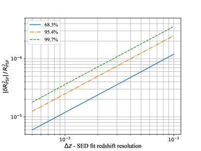
Figure 17: The relative error in the effective PSF size $R_{\rm PSF}^{2}$ as a function of the redshift resolution used in the SED template fitting method. $R_{\rm PSF}^{2}$ is estimated using the r,i,z bands with no magnitude noise and without photo-z priors. The three lines show the $1-\sigma,2-\sigma$ and $3-\sigma$ limits of the $\delta R_{\rm PSF}^{2}$ distribution.

Template fitting algorithms (e.g. BPZ; Benítez, 2000) compare observations with a model on a two-dimensional grid of redshift and galaxy SED. The number of SEDs depends on the number of templates used and the number of interpolations between consecutive templates (we use 2). Given the rather poor precision in redshift ($\sigma_{z}\sim 0.03-0.05$) that can be achieved using broad-band data, the redshift sampling is typically $\Delta z\approx 0.01$ in order to minimize runtime. Increasing the redshift resolution is straightforward as it only requires modifying a configuration parameter, but the runtime increases roughly linearly with the number of evaluations in redshift. Given the sensitivity to photometric redshift errors (see §3.2) we check here if the default setting is sufficient to estimate the effective PSF size.

To do so, we determine $\delta R^{2}_{\rm PSF}/R^{2}_{\rm PSF}$ as a function of the redshift resolution $\Delta z$. To isolate the effect of the redshift resolution we consider an idealised situation with no measurement errors and fit the simulated r,i,z data without photo-z priors. For $\Delta z=0.01$ the resulting average relative bias is below $10^{-6}$ (not shown), which is two orders of magnitude below requirements. Instead we show in Fig. 17 the $1-\sigma,2-\sigma,3-\sigma$ limits of the $\delta R_{\rm PSF}^{2}$ distribution, which also captures the tails of the distribution of $\delta R_{\rm PSF}^{2}$ values. Fitting with a resolution $\Delta z=0.01$ is thus sufficient to avoid introducing an additional bias, which we also verified with noisy simulations.

Appendix B $R^{2}$ bias calibration technique

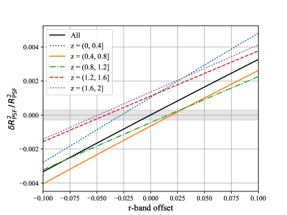
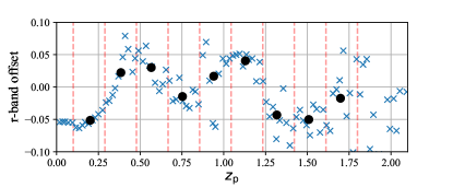
Figure 18: Top: $\delta R^{2}_{\rm PSF}/R^{2}_{\rm PSF}$ in the calibration sample as a function of the applied r-band offset. The training uses the r-i and i-z colours from stars and the offset is included in the r-i colour. One line shows the full sample (All), while the rest split in photometric redshift bins. A shaded horizontal band marks the Euclid requirement. Bottom: The optimal r-band offset as a function of redshift. The circles is the r-band offset in the bins ($\Delta z=0.18)$ marked with vertical lines, while the crosses use a resoltion of $\Delta z=0.02$.

The scikit-learn library includes many algorithms for regression. Several other algorithms (tree based and nearest neighbours) performed well for the full sample of galaxies when applied to r,i,z observations of stars. Unfortunately, all resulted in a strong variation of the bias in effective PSF size with redshift, resulting in the need for an additional correction. There are multiple avenues to reduce these residual biases using a calibration sample of simulated galaxies. For instance, one could determine the offsets as a function of color or redshift. However, reliably predicting a small bias based on noisy input is difficult. We explored various approaches, but were unable to achieve the required performance.

Interestingly, we found that introducing a small r-band magnitude offset in the algorithm to correct the predicted value of $R^{2}_{\rm PSF}$ yielded satisfactory results. Figure 18 shows a linear dependence of $\delta R^{2}_{\rm PSF}/R^{2}_{\rm PSF}$ to an r-band shift for different redshifts when training on stars with the r,i,z bands. We found good performance when we consider nine redshift bins; as shown in the bottom panel of Fig 18 the resulting r-band offset varies fairly smoothly with redshift. A finer binning in redshift (as indicated by the crosses) shows that the actual variation with redshift is more erratic. This is naturally captured when training on galaxy templates alone. Hence the redshift sample $\Delta z$ can be considered a parameter that regulates the importance of the galaxy templates: no binning corresponds to training on stars, whereas $\Delta z=0$ is equivalent to training on the galaxy templates. We found that our choice of $\Delta z=0.18$ provided a good compromise that performs well for the prediction of the effective PSF size of a galaxy.

Appendix C Performance without z-band observations

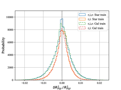
Figure 19: Histogram of $\delta R_{\rm PSF}^{2}/R_{\rm PSF}^{2}$ values when training using either r,i,z (blue) or r and i (red) data. The solid lines correspond to the case where the algorithm is trained on stars, whereas the dashed lines show the results when training on the galaxy simulations. The vertical band marks the Euclid requirement for the mean bias.

When training on galaxies, the best performance was obtained when we used $r$ and $i$ photometry only, which can be understood because the VIS passband overlaps only with the blue half of the full $z$-band. It is therefore interesting to examine whether $z$-band data can be omitted, especially given the relatively large amount of observing time needed to obtain these data from the ground.

To compare the performances of the various filter combinations, we show in Fig. 19 the distributions of $\delta R_{\rm PSF}^{2}/R^{2}_{\rm PSF}$. The main impact of omitting the $z$-band is an increase in the scatter, but this has a negligible impact on the overall precision of the weak lensing analysis. We note that the approach discussed in Appendix B also works well using only $r$ and $i$ data (see Fig. 20).

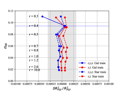
Figure 20: The effect of the magnitude depth on the photometric redshift and the $R_{\rm PSF}^{2}$ bias. The points indicate the ratio in the exposure times relative to the fiducial setup (with values indicated). The blue lines indicate the results when training using the r,i,z data, whereas the red lines are for the case where the z-band is omitted. The solid lines are for the results when the algorithm is trained on stars, and the dashed lines are when the simulated galaxies are used to train. Note that when the z-band is omitted, it is also not used in the photo-$z$ determination. The vertical band marks the Euclid requirement bias in effective PSF size.

The depth of the supporting multi-band photometry for Euclid is determined by the need for sufficiently precise photometric redshifts, but also affects our ability to determine the effective PSF size. It is therefore important to examine the impact of changes in depth (and filter coverage) on both of these key aspects of the lensing measurements.

This is captured in Fig. 20 which shows $\sigma_{68}$ and $\delta R_{\rm PSF}^{2}/R_{\rm PSF}^{2}$ as a function of exposure time, where $\sigma_{68}$ is the (average two-sided) 68 per cent limit of $(z_{p}-z_{s})$, which corresponds to $1-\sigma$ for a Gaussian distribution, but is less sensitive to the outliers than the rms. The magnitude errors enter in the estimates of the photometric redshift and the effective PSF size. In the figure ‘r’ indicates the relative change in exposure time in the r,i,z bands, relative to the nominal values used throughout the paper. The photo-$z$ estimate does not include the Euclid VIS-band. Not surprisingly, longer exposures significantly decrease the photo-$z$ scatter and vice versa. We also show results without $z$-band observations and find only small differences in the precision of the photometric redshifts and the bias in effective PSF size.

The most noticeable result is how insensitive $\delta R_{\rm PSF}^{2}/R_{\rm PSF}^{2}$ is to the change in depth. For the fiducial exposures all lines are well within the requirement. This can be attributed to the calibration sample, which also simulates the measurement noise: when changing the exposure time we also change the noise level in the calibration sample and the calibration therefore helps to remove the noise bias. We note, however, that this does increase the noise in the PSF estimate. Nonetheless it is clear that the required precision in the determination of photometric redshifts is the main driver for the depth of the photometric data.

References

- Becker et al. (2016) Becker M. R. et al., 2016, Phys. Rev. D, 94, 022002
- Benítez (2000) Benítez N., 2000, ApJ, 536, 571
- Bonnett (2015) Bonnett C., 2015, MNRAS, 449, 1043
- Coe et al. (2006) Coe D., Benítez N., Sánchez S. F., Jee M., Bouwens R., Ford H., 2006, AJ, 132, 926
- Coleman, Wu & Weedman (1980) Coleman G. D., Wu C.-C., Weedman D. W., 1980, ApJS, 43, 393
- Collister & Lahav (2004) Collister A. A., Lahav O., 2004, PASP, 116, 345
- Cropper et al. (2013) Cropper M. et al., 2013, MNRAS, 431, 3103
- Cypriano et al. (2010) Cypriano E. S., Amara A., Voigt L. M., Bridle S. L., Abdalla F. B., Réfrégier A., Seiffert M., Rhodes J., 2010, MNRAS, 405, 494
- Finkbeiner et al. (2016) Finkbeiner D. P. et al., 2016, ApJ, 822, 66
- Heymans et al. (2013) Heymans C. et al., 2013, MNRAS, 432, 2433
- Heymans et al. (2006) Heymans C. et al., 2006, MNRAS, 368, 1323
- Heymans et al. (2012) Heymans C. et al., 2012, MNRAS, 427, 146
- Hildebrandt et al. (2017) Hildebrandt H. et al., 2017, MNRAS, 465, 1454
- Hoekstra & Jain (2008) Hoekstra H., Jain B., 2008, Annual Review of Nuclear and Particle Science, 58, 99
- Hunter (2007) Hunter J., 2007, Computing in Science Engineering, 9, 90
- Ilbert et al. (2006) Ilbert O. et al., 2006, A&A, 457, 841
- Israel et al. (2015) Israel H. et al., 2015, MNRAS, 453, 561
- Jee et al. (2016) Jee M. J., Tyson J. A., Hilbert S., Schneider M. D., Schmidt S., Wittman D., 2016, ApJ, 824, 77
- Joachimi et al. (2015) Joachimi B. et al., 2015, Space Sci. Rev., 193, 1
- Jones et al. (2001) Jones E., Oliphant T., Peterson P., et al., 2001, SciPy: Open source scientific tools for Python. [Online; accessed 2015-10-21]
- Kilbinger (2015) Kilbinger M., 2015, Reports on Progress in Physics, 78, 086901
- Kirk et al. (2015) Kirk D. et al., 2015, Space Sci. Rev., 193, 139
- Kuijken et al. (2015) Kuijken K. et al., 2015, MNRAS, 454, 3500
- Laureijs et al. (2011) Laureijs R. et al., 2011, preprint(arXiv:1110.3193)
- LSST Science Collaboration et al. (2009) LSST Science Collaboration et al., 2009, preprint(arXiv:0912.0201)
- Martí et al. (2014) Martí P., Miquel R., Castander F. J., Gaztañaga E., Eriksen M., Sánchez C., 2014, MNRAS, 442, 92
- Massey et al. (2013) Massey R. et al., 2013, MNRAS, 429, 661
- Massey et al. (2014) Massey R. et al., 2014, MNRAS, 439, 887
- McKinney (2010) McKinney W., 2010, in Proceedings of the 9th Python in Science Conference, van der Walt S., Millman J., eds., pp. 51 – 56
- Meyers & Burchat (2015) Meyers J. E., Burchat P. R., 2015, ApJ, 807, 182
- Pedregosa et al. (2012) Pedregosa F. et al., 2012, preprint(arXiv:1201.0490)
- Perlmutter et al. (1999) Perlmutter S. et al., 1999, ApJ, 517, 565
- Perryman et al. (2001) Perryman M. A. C. et al., 2001, A&A, 369, 339
- Pérez & Granger (2007) Pérez F., Granger B., 2007, Computing in Science Engineering, 9, 21
- Pickles (1998) Pickles A. J., 1998, PASP, 110, 863
- Riess et al. (1998) Riess A. G. et al., 1998, AJ, 116, 1009
- Semboloni et al. (2013) Semboloni E. et al., 2013, MNRAS, 432, 2385
- Spergel et al. (2015) Spergel D. et al., 2015, preprint(arXiv:1503.03757)
- Voigt et al. (2012) Voigt L. M., Bridle S. L., Amara A., Cropper M., Kitching T. D., Massey R., Rhodes J., Schrabback T., 2012, MNRAS, 421, 1385
- Weinberg et al. (2013) Weinberg D. H., Mortonson M. J., Eisenstein D. J., Hirata C., Riess A. G., Rozo E., 2013, Phys. Rep., 530, 87