Abstract

Semi-hard processes in the large center-of-mass energy limit offer us an exclusive chance to test the dynamics behind strong interactions in kinematical sectors so far unexplored, the high luminosity and the record energies of the LHC providing us with a richness of useful data. In the Regge limit, $s\gg|t|$, fixed-order calculations in perturbative QCD based on collinear factorisation miss the effect of large energy logarithms, which are so large to compensate the small QCD coupling $\alpha_{s}$ and must therefore be accounted for to all perturbative orders. The BFKL approach represents the most powerful tool to perform the resummation to all orders of these large logarithms both in the LLA, which means inclusion of all terms proportional to $(\alpha_{s}\ln(s))^{n}$, and NLA, which means inclusion of all terms proportional to $\alpha_{s}(\alpha_{s}\ln(s))^{n}$. The inclusive hadroproduction of forward jets with high transverse momenta separated by a large rapidity gap at the LHC, the so-called Mueller–Navelet jets, has been one of the most studied reactions so far. Interesting observables associated to this process are the azimuthal correlation momenta, showing a very good agreement with experimental data at the LHC. However, new BFKL-sensitive observables should be considered in the context of the LHC physics program. With the aim the to further and deeply probe the dynamics of QCD in the Regge limit, we give phenomenological predictions for four distinct semi-hard process. On one hand, we continue the analysis of reactions with two objects identified in the final state $(i)$ by addressing open problems in the Mueller–Navelet sector and $(ii)$ by studying the inclusive dihadron production in the full NLA BKFL accuracy. Hadrons can be detected at the LHC at much smaller values of the transverse momentum than jets, allowing us to explore an additional kinematical range, complementary to the one studied typical of Mueller–Navelet jets. Furthermore, this process permits to constrain not only the parton distribution functions for the initial proton, but also the parton fragmentation functions describing the detected hadron in the final state. On the other hand, we show how inclusive multi-jet production processes allow us to define new, generalised and suitable BFKL observables, where transverse momenta and rapidities of the tagged jets, well separated in rapidity from each other, appear in new combinations. We give the first phenomenological predictions for the inclusive three-jet production, encoding the effects of higher-order BFKL corrections. Then, making use of the same formalism, we present the first complete BFKL analysis for the four-jet production.

Sintesi in lingua italiana

Per quanto una teoria fisica possa apparire complessa e formalmente ardua l’origine della sua eleganza risiede quasi sempre in un’idea semplice e concreta. Il Modello Standard (MS) delle particelle elementari, solidamente edificato sull’esistenza di costituenti fondamentali di natura fermionica che interagiscono tra loro attraverso lo scambio di bosoni vettori intermedi, tra gli esempi pi significativi. All’interno del MS, la Cromodinamica Quantistica (QCD) la teoria che descrive le interazioni forti tra i quark, particelle costituenti di natura fermionica, e i gluoni, bosoni mediatori dell’interazione stessa.

Nel limite di alte energie nel centro di massa $\sqrt{s}$, lo studio dei processi semiduri (ovvero quei processi caratterizzati da scale dure molto maggiori della scala della QCD $\Lambda_{\rm QCD}$ ma, al contempo, notevolmente inferiori rispetto a $\sqrt{s}$) permette senza dubbio di effettuare prove stringenti della dinamica delle interazioni forti in regimi cinematici ad ora inesplorati. Nel limite di Regge ($s\gg|t|$, con $t$ la variabile di Mandelstam rappresentante il quadrato della quantit di momento trasferito), le predizioni teoriche di QCD perturbativa ad ordine fissato, basate sulla fattorizzazione collineare, non possono tener conto dell’effeto non trascurabile dei logaritmi in energia, il cui contributo tale da compensare quello della costante d’accoppiamento della QCD $\alpha_{s}$ e, per tale ragione, deve essere tenuto in conto a tutti gli ordini dello sviluppo perturbativo. L’approccio Balitsky–Fadin–Kuraev–Lipatov (BFKL) rappresenta di certo lo strumento pi potente in grado di risommare a tutti gli ordini il contributo di tali logaritmi, sia in approssimazione logaritmica dominante (LLA), ossia risommazione di tutti i termini proporzionali a $(\alpha_{s}\ln(s))^{n}$, sia in quella sottodominante (NLA), ossia risommazione dei fattori del tipo $\alpha_{s}(\alpha_{s}\ln(s))^{n}$.

Il processo di produzione inclusiva “in avanti” di jet con alto momento trasverso e separati da un grande intervallo di rapidit , meglio noto come produzione di jet di Mueller–Navelet, , ad oggi, tra le reazioni pi studiate. La ragione della sua popolarit in ambito scientifico risiede soprattutto nell’aver fornito la possibilit di definire i momenti di correlazione azimutale, osservabili infrared-safe le cui predizioni teoriche sono in buon accordo con i dati sperimentali ottenuti al Large Hadron Collider (LHC). È tuttavia necessario che nuove osservabili, sensibili alla dinamica BFKL, vengano considerate nell’ambito della fenomenologia di LHC.

Perseguendo lo scopo di approfondire ed estendere la conoscenza della dinamica delle interazioni forti nel limite di Regge, si propone lo studio di quattro distinti processi semiduri.

Nella prima parte dell’analisi fenomenologica presentata, ci si propone di continuare l’indagine di processi caratterizzati da due oggetti identificati nello stato finale, proseguendo lo studio dei problemi aperti nel processo di produzione di jet di Mueller–Navelet e, nello stesso tempo, affiancando ad esso quello della produzione inclusiva di una coppia adrone-antiadrone (dihadron system) carico leggero del tipo $\pi^{\pm},K^{\pm},p,\bar{p}$, entrambi caratterizzati da alto momento trasverso e fortemente separati in rapidit . La possibilit di rivelare gli adroni ad LHC a valori del momento trasverso di gran lunga inferiori rispetto ai jet consente di esplorare un settore cinematico complementare a quello studiato attraverso il canale di Mueller–Navelet. La produzione di adroni offre, inoltre, la possibilit di investigare simultaneamente il comportamento di oggetti non perturbativi, quali le funzioni di distribuzione partonica (PDF) del protone nello stato iniziale e le funzioni di frammentazione (FF) caratterizzanti l’adrone rivelato nello stato finale.

Nella seconda parte della tesi, si pone e si evidenzia come lo studio della produzione di pi jet nello stato finale (multi-jet production) fornisca la possibilit di generalizzare le osservabili definite nel caso di processi con due oggetti nello stato finale, costruendone delle nuove, maggiormente sensibili alla dinamica BFKL a causa della loro dipendenza da momenti trasversi e rapidit dei jet rivelati nelle regioni centrali dei rivelatori. È presentata la prima analisi fenomenologica sulla produzione di tre jet, tenendo conto degli effetti dovuti all’inclusione delle correzioni d’ordine superiore in risommazione BFKL. Infine, facendo uso dello stesso formalismo, viene presentato il primo studio completo sulla produzione di quattro jet.

Chapter 1 Introduction

Insofar as a physical theory may appear complex and formally arduous, the origin of its elegance lies almost always on a simple and concrete idea. The Standard Model (SM) of elementary particles, solidly built up on the existence of fermionic fundamental constituents, their mutual interaction being mediated via the exchange of intermediate vector bosons, represents one of the most significant examples. Inside the SM, Quantum Chromodynamics (QCD) is the theory of strong interactions, describing how fermionc quarks and bosonic gluons, the elementary constituents of hadrons , such as the proton and the neutron, interact with each other. What makes QCD a challenging sector surrounded by a broad and constant interest in its phenomenology, is the duality between non-perturbative and perturbative aspects which comes from the coexistence of two peculiar and concurrent properties, as confinement and asymptotic freedom. The striking feature of confinement is the increasing of the strong coupling $\alpha_{s}$ with distance. This means that hadrons are described by bound states of quarks and gluons, which cannot be described at the hand of any perturbative calculation. Conversely, the short-distance regime is ruled by asymptotic freedom, so that quarks and gluons behave as quasi-free particles, making it possible to use perturbative approaches.

The high luminosity and the record energies of the Large Hadron Collider (LHC) provide us with a wealth of useful data. A peerless opportunity to test strong interactions in this so far unexplored kinematical configuration of large center-of-mass energy is given by the study of semi-hard processes, i.e. hard processes in the kinematical region where the center-of-mass energy squared $s$ is substantially larger than one or more hard scales $Q^{2}_{i}$ (large squared transverse momenta, large squared quark masses and/or $t$), $s\gg Q^{2}_{i}$, which satisfy in turn $Q^{2}_{i}\gg\Lambda_{\rm QCD}^{2}$, with $\Lambda_{\rm QCD}$ the QCD scale. In the kinematical regime , known as Regge limit (see also Section 2.1), $s\gg|t|$, fixed-order calculations in perturbative QCD based on collinear factorisation  miss the effect of large energy logarithms, entering the perturbative series with a power increasing with the order and thus compensating the smallness of the coupling $\alpha_{s}$. The Balitsky–Fadin–Kuraev–Lipatov (BFKL) approach [BFKL, BFKL_2, BFKL_3, BFKL_4] serves as the most powerful tool to perform the all-order resummation of these large energy logarithms both in the leading approximation (LLA), which means inclusion of all terms proportional to $(\alpha_{s}\ln(s))^{n}$, and the next-to-leading approximation (NLA), which means inclusion of all terms proportional to $\alpha_{s}(\alpha_{s}\ln(s))^{n}$. In the BFKL formalism, it is possible to express the cross section of an LHC process falling in the domain of perturbative QCD as the convolution between two impact factors, which describe the transition from each colliding proton to the respective final-state object, and a process-independent Green’s function. The BFKL Green’s function obeys an integral equation, whose kernel is known at the next-to-leading order (NLO) both for forward scattering (i.e. for $t=0$ and colour singlet in the $t$-channel) [Fadin:1998py, Ciafaloni:1998gs] and for any fixed (not growing with energy) momentum transfer $t$ and any possible two-gluon colour state in the $t$-channel [Fadin:1998jv, Fadin:2000kx, FF05, FF05_2].

The too low $\sqrt{s}$, bringing to small rapidity intervals among the tagged objects in the final state, had been so far the weakness point of the search for BFKL effects. Furthermore, too inclusive observables were considered. A striking example is the growth of the hadron structure functions at small Bjorken-$x$ values in Deep Inelastic Scattering (DIS). Although NLA BFKL predictions for the structure function $F_{2,L}$ have shown a good agreement with the HERA data [Hentschinski:2012kr, Hentschinski:2013id], also other approaches can fit these data. The LHC record energy, together with the good resolution in azimuthal angles of the particle detectors, can address these issues: on one side larger rapidity intervals in the final state are reachable, allowing us to study a kinematical regime where it is possible to disentangle the BFKL dynamics from other resummations; on the other side, there is enough statistics to define and investigate more exclusive observables, which can, in principle, be only described by the BFKL framework.

With this aim, the production of two jets featuring transverse momenta much larger than $\Lambda^{2}_{\rm QCD}$ and well separated in rapidity, known as Mueller–Navelet jets, was proposed [Mueller:1986ey] as a tool to investigate semi-hard parton scatterings at a hadron collider. This reaction represents a unique venue where two main resummations, collinear and BFKL ones, play their role at the same time in the context of perturbative QCD. On one hand, the rapidity ranges in the final state are large enough to let the NLA BFKL resummation of the energy logarithms come into play. The process-dependent part of the information needed to build up the cross section is encoded in the impact factors (the so-called “jet vertices”), which are known up to NLO  [Fadin:1999de, Fadin:1999df, Ciafaloni:1998kx, Ciafaloni:1998hu, Bartels:2001ge, Bartels:2002yj, Caporale:2011cc, Ivanov:2012ms, Colferai:2015zfa]. On the other hand, the jet vertex can be expressed, within collinear factorisation at the leading twist, as the convolution of the PDF of the colliding proton, obeying the standard DGLAP evolution, with the hard process describing the transition from the parton emitted by the proton to the forward jet in the final state.

A large number of numerical analyses [Colferai:2010wu, Angioni:2011wj, Caporale:2012ih, Ducloue:2013wmi, Ducloue:2013bva, Caporale:2013uva, Ducloue:2014koa, Caporale:2014gpa, Ducloue:2015jba, Caporale:2015uva, Chachamis:2015crx] has appeared so far, devoted to NLA BFKL predictions for the Mueller–Navelet jet production process. All these studies are involved in calculating cross sections and azimuthal angle correlations [DelDuca:1993mn, Stirling:1994he] between the two measured jets, i.e. average values of $\cos{(n\phi)}$, where $n$ is an integer and $\phi$ is the angle in the azimuthal plane between the direction of one jet and the direction opposite to the other jet, and ratios of two such cosines [Vera:2006un, Vera:2007kn]. Recently [Khachatryan:2016udy], the CMS Collaboration presented the first measurements of the azimuthal correlation of the Mueller–Navelet jets at $\sqrt{s}=7$ TeV at the LHC. Further experimental studies of the Mueller–Navelet jets at higher LHC energies and larger rapidity intervals, including also the effects of using asymmetric cuts for the jet transverse momenta, are expected.

In order to reveal the dynamical mechanisms behind partonic interactions in the Regge limit, new observables, sensitive to the BFKL dynamics and more exclusive than the Mueller–Navelet ones, need to be proposed and considered in the next LHC analyses.

A first step in this direction is the study of another reaction, less inclusive than Mueller–Navelet jets although sharing with it the theoretical framework, i.e. the inclusive detection of two charged light hadrons (a dihadron system) $\pi^{\pm},K^{\pm},p,\bar{p}$ having high transverse momenta and well separated in rapidity. Since the key ingredient beyond the NLA BFKL Green’s function, i.e. the process-dependent vertex describing the production of an identified hadron, was obtained with NLA in [hadrons], it is possible to study this process in the NLA BFKL approach. After the renormalisation of the QCD coupling and the ensuing removal of the ultraviolet divergences, soft and virtual infrared divergences cancel each other, whereas the surviving infrared collinear ones are compensated by the collinear counterterms related to the renormalisation of PDFs for the initial proton and parton fragmentation functions (FFs) describing the detected hadron in the final state within collinear factorisation. All the theoretical criteria are thus met to give infrared-safe NLA predictions, thus making of this process an additional clear channel to test the BFKL dynamics at the LHC. The fact that hadrons can be detected at the LHC at much smaller values of the transverse momentum than jets, allows to explore a kinematical range outside the reach of the Mueller–Navelet channel, so that the reaction can be considered complementary to Mueller–Navelet jet production. Furthermore, it represents the best context to simultaneously constrain both PDFs and FFs.

The second advance towards further and deeply probing BFKL dynamics is the study of inclusive multi-jet production processes where, besides two external jets typical of Mueller–Navelet reactions, the tagging of further jets in more central regions of the detectors and with a relative separation in rapidity from each other is demanded. This allows for the study of even more differential distributions in the transverse momenta, azimuthal angles and rapidities of the central jets, by generalising the two-jet azimuthal correlations $R_{nm}\equiv\cos{(n\phi)}/\cos{(m\phi)}$ to new, suitable BFKL observables sensitive to the azimuthal configurations of the tagged extra particles.

Aware of the importance to pursue the phenomenological paths traced above, we work toward the goal of giving testable predictions on the QCD semi-hard sector by proposing the study of four distinct processes. First, we continue the study of Mueller–Navelet jets by addressing issues that still wait to be answered, as the comparison of BFKL with NLO fixed-order perturbative approaches [Celiberto:2015yba] and a 13 TeV analysis, together with the study of the effect of imposing dynamic constraints in the central rapidity region [Celiberto:2016ygs]. Second, we will give the first phenomenological results for cross sections and azimuthal correlations in the inclusive dihadron production. Third, we will show how the inclusive three-jet production process allows to define in a very natural and elegant way new, generalised and suitable BFKL observables. Finally, we will investigate the inclusive four-jet production, extending the BFKL formalism defined and used in the three-jet case.

This thesis is organised as follows. In Chapter 2 a brief overview of the BFKL approach is given, while phenomenological predictions at LHC energies for the considered semi-hard processes are shown in the next four Chapters. In particular, Mueller–Navelet jets and the inclusive dihadron production are discussed in Chapters 3 and 4, respectively, showing the lastest results at full NLA accuracy, together with a study on the effect of using different values for the renormalisation and factorisation scales. In Chapter 5 the first complete analysis of the inclusive three-jet production process is presented, including the effects of higher-order BFKL corrections. The four-jet production process is investigated in Chapter LABEL:chap:4j, giving the first results at LLA accuracy. In each Chapter devoted to phenomenology a related summary Section is provided, while the general Conclusions, together with Outlook, are drawn in Chapter LABEL:chap:conclusions.

Chapter 2 The BFKL resummation

2.1 The Regge theory

In 1959 the Italian physicist T. Regge [Regge:1959mz] found that, when considering solutions of the Schrödinger equation for non-relativistic potential scattering, it can be advantageous to regard the angular momentum, $l$, as a complex variable. He showed that, for a wide class of potentials, the only singularities of the scattering amplitude in the complex $l$-plane are poles, called Regge poles [Collins, Barone-Predazzi] after him. If these poles appear in coincidence with integer values of $l$, they correspond to bound states or resonances and turn out to be important for the analytic properties of the amplitudes. They occur at the values given by the relation

$$l=\alpha(k)\;,$$ (2.1)

where $\alpha(k)$ is a function of the energy, known as Regge trajectory or Reggeon. Each class of bound states or resonances is related to a single trajectory like (2.1). The energies of these states are obtained from Eq. (2.1), giving physical (integer) values to the angular momentum $l$. The extension of the Regge’s approach to high-energy particle physics was formerly due to Chew and Frautschi [Chew:1961ev] and Gribov [Gribov:1961fr], but many other physicists gave their contribution to the theory and its applications. Using the general properties of the $S$-matrix, the relativistic partial wave amplitude $\mathcal{A}_{l}(t)$ can be analytically continued to complex $l$ values in a unique way. The resulting function, $A(l,t)$, shows simple poles at

$$l=\alpha(t)\;.$$ (2.2)

Each pole contributes to the scattering amplitude with a term which asymptotically behaves (i.e. for $s\to+\infty$ and for fixed $t$) as

$$A(s,t)\sim s^{\alpha(t)}\;,$$ (2.3)

where $s$ and $-t$ are the square of the center-of-mass energy and of the momentum transfer, respectively. The leading singularity in the $t$-channel is the one with the largest real part, and rules the asymptotic behaviour of the scattering amplitude in the $s$-channel. The triumph of Regge theory in its simplest form, i.e. the fact that a large class of processes is accurately described by such simple predictions as Eq. (2.3), was simply surprising.

2.1.1 The Pomeron

Regge theory belongs to the class of the so-called $t$-channel models. They describe hadronic processes in terms of the exchange of “some objects” in the $t$-channel. In the Regge theory a Reggeon plays the same role as an exchanged virtual particle in a tree-level perturbative process, with the important difference that the Reggeon represents a whole class of resonances, instead of a single particle. In the limit of large $s$, a hadronic process is governed by the exchange of one or more Reggeons in the $t$-channel. The exchange of Reggeons instead of particles gives rise to scattering amplitudes of the type of Eq. (2.3). Using the optical theorem [optical_theorem_Newton] together with Eq. (2.3), we can write the Regge total cross section:

$$\sigma_{\rm TOT}\simeq\frac{{\rm Im}\,A(s,t=0)}{s}\simeq s^{\alpha(0)-1}\;.$$ (2.4)

We know from experiments that hadronic total cross sections, as a function of $s$, are rather flat around $\sqrt{s}\simeq(10\div 20)$ GeV and rise slowly as $\sqrt{s}$ increases. If the considered process is described by the exchange of a single Regge pole, then it follows that the intercept $\alpha(0)$ of the exchanged Reggeon is greater than 1, leading to the power growth with energy of the cross section in Eq. (2.4). This Reggeon is called Pomeron, in honour of I.Ya. Pomeranchuk. Particles which would provide the resonances for integer values of $\alpha(t)$ for $t>0$ have not been conclusively identified. Natural candidates in QCD are the so-called glueballs. The Pomeron trajectory represents the dominant trajectory in elastic and diffractive processes, namely reactions featuring the exchange of vacuum quantum numbers in the $t$-channel. The power growth of the cross section violates the Froissart bound [Froissart:1961ux] and hence the unitarity, which has to be restored through unitarisation techniques (see for instance Ref. [Forshaw-Ross] and references therein).

2.2 Towards the BFKL equation

The BFKL equation [BFKL, BFKL_2, BFKL_3, BFKL_4] made the grade when the growth of the $\gamma^{*}p$ cross section at increasing energy, predicted by Balitsky, Fadin, Kuraev, and Lipatov, was experimentally confirmed at HERA. Therefore this equation is usually associated with the evolution of the unintegrated gluon distribution.

The PDF evolution with $\tau=\ln\left(Q^{2}/\Lambda_{\rm QCD}\right)$ is determined by the DGLAP equations [DGLAP, DGLAP_2, DGLAP_3, DGLAP_4, DGLAP_5], which allow to resum to all orders collinear logarithms $\ln Q^{2}$ picked up from the region of small angles between parton momenta. There is another class of logarithms to be taken into account: soft logarithms which originate from ratios of parton energies and are present both in PDFs and in partonic cross sections. At small values of the ratio $x=\ln Q^{2}/s$ soft logarithms are even larger than collinear ones.

The BFKL approach describes QCD scattering amplitudes in the limit of small $x$, $s\gg|t|$, and $t$ not growing with $s$ (Regge limit). The evolution equation for the unintegrated gluon distribution appears in this approach as a particular result for the imaginary part of the forward scattering amplitude ($t=0$ and vacuum quantum numbers in the $t$-channel). This approach was developed (and is more suitable) for the description of processes with just one hard scale, such as $\gamma^{*}\gamma^{*}$ scattering with both photon virtualities of the same order, where the DGLAP evolution is not appropriate. The BFKL approach relies on gluon Reggeisation, which can be described as the appearance of a modified propagator in the Feynman gauge, of the form [Barone-Predazzi]

$$D_{\mu\nu}(s,q^{2})=-i\frac{g_{\mu\nu}}{q^{2}}\left(\frac{s}{s_{0}}\right)^{\alpha_{g}(q^{2})-1}\;,$$ (2.5)

where $\alpha_{g}(q^{2})=1+\epsilon(q^{2})$ is the gluon Regge trajectory.

2.2.1 Gluon Reggeisation

The Reggeisation of an elementary particle featuring spin $j_{0}$ and mass $m$ was introduced in Ref. [Gell-Mann:ep_III] and it means [IFL] that, in the Regge limit, a factor $s^{j(t)-j_{0}}$, with $j_{0}\equiv j(m^{2})$ appears in Born amplitudes with exchange of this particle in the $t$-channel. This phenomenon was discovered originally in QED via the backward Compton scattering [Gell-Mann:ep_III]. It was called Reggeisation because just such form of amplitudes is given by the Regge poles (moving poles in the complex $l$-plane [Regge:1959mz]). In contrast to QED, where the electron reggeises in perturbation theory [Gell-Mann:ep_III], but the photon remains elementary [Mandelstam:PR137B949:1965], in QCD the gluon reggeises [BFKL, BFKL_2, Grisaru:1973vw, Grisaru:1974cf, Lipatov:1976zz] as well as the quark [Fadin:1976nw, Fadin:1977jr, Bogdan:2002sr, Kotsky:2002aq]. Therefore QCD is the unique theory where all elementary particles reggeise.

Reggeisation represents a key-ingredient for the theoretical description of high-energy processes with fixed momentum transfer. Gluon Reggeisation is particularly important, because cross sections non-decreasing with energy are provided by gluon exchanges, and it determines the form of QCD amplitudes in the Regge limit. The simplest realisation of the gluon Reggeisation happens in the elastic process $A+B\to A^{\prime}+B^{\prime}$,

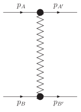
Figure 2.1: Diagrammatical representation of the process $A+B\to A^{\prime}+B^{\prime}$ with colour octet in the $t$-channel. The waggle line represents the Reggeised gluon exchange.

where amplitudes with a colour-octet exchange in the $t$-channel and negative signature (see Fig. 2.1 for a diagrammatical representation) assume the form

$$\left(\mathcal{A}_{8}\right)^{A^{\prime}B^{\prime}}_{AB}=\Gamma^{c}_{A^{\prime}A}\frac{s}{t}\left[\left(\left(\frac{s}{-t}\right)^{\omega(t)}+\left(\frac{-s}{-t}\right)^{\omega(t)}\right)\right]\Gamma^{c}_{B^{\prime}B}\;,$$ (2.6)

where

$$s=(p_{A}+p_{B})^{2}\;,$$ (2.7)

$$t=q^{2}\;,$$

$$q=p_{A}-p_{A^{\prime}}\;,$$

$\omega(t)$ is the gluon trajectory, $c$ is the colour index, and $\Gamma^{c}_{B^{\prime}B}$ are the particle-particle-Reggeon (PPR) vertices which are independent of $s$. The factorisation given in Eq. (2.6) represents the analytical structure of the scattering amplitude, which is quite simple in the elastic case. It is valid both in the LLA and in the NLA. In particular, it holds when one of the particles $A^{\prime}$ and $B^{\prime}$ is replaced by a jet. In general the PPR vertex can be written in the form $\Gamma^{C}_{P^{\prime}P}=g_{s}\left\langle P^{\prime}|T^{c}|P\right\rangle\Gamma_{P^{\prime}P}$, where $g_{s}$ is the QCD coupling and $\left\langle P^{\prime}|T^{c}|P\right\rangle$ is the matrix element of the colour-group generator in the fundamental (adjoint) representation for quarks (gluons). In the LLA this form of amplitude was proved in Refs. [BFKL, BFKL_2, BFKL_3, BFKL_4]. In this approximation, the helicity $\lambda_{p}$ of the scattered particle $P$ is a conserved quantity, so $\Gamma^{(0)}_{P^{\prime}P}$ is given by $\delta_{\lambda_{P^{\prime}}\lambda_{P}}$ and the Reggeised gluon trajectory is calculated with 1-loop accuracy [Fadin:1998sh], having so

$$\omega(t)\simeq\omega^{(1)}(t)=\frac{g_{s}^{2}t}{(2\pi)^{(D-1)}}\frac{N_{c}}{2}\int\frac{d^{D-2}k_{\bot}}{k_{\bot}^{2}(q-k_{\bot})^{2}_{\bot}}$$ (2.8)

$$=-\frac{g_{s}^{2}N_{c}\Gamma(1-\epsilon)}{(4\pi)^{\frac{D}{2}}}\frac{\Gamma^{2}(\epsilon)}{\Gamma(2\epsilon)}\left(\vec{q}^{2}\right)^{\epsilon}$$

where $t=q^{2}\approx q_{\bot}^{2}$, $D=4+2$ is the space-time dimension and $N_{c}$ is the number of QCD colours. The $\epsilon$ parameter has been introduced in order to regularise the infrared divergences, while the integration is done in a $(D-2)$-dimensional space, orthogonal to the momenta of the initial colliding particles $p_{A}$ and $p_{B}$. The gluon Reggeisation determines also the form of inelastic amplitudes in the multi-Regge kinematics (MRK), namely where all particles are strongly ordered in the rapidity space with limited transverse momenta and the squared invariant masses $s_{ij}=(k_{i}+k_{j})^{2}$ of any pair of produced particles $i$ and $j$ are large and increasing with $s$. This kinematics gives the leading contribution to QCD cross sections. In the LLA, there are exchanges of vector particles (QCD gluons) in all channels. In the NLA, as opposed to LLA, MRK is not the solely contributing kinematic configuration. It can happen then one (and just one) of the produced particles can have a fixed (not increasing with $s$) invariant mass, i.e. components of this pair can have rapidities of the same order. This is known as quasi-multi-Regge-kinematics (QMRK) [Fadin:1989kf]. In the NLA the expression given in Eq. (2.6) was checked initially at the first three perturbative orders [Fadin:1995dd, Fadin:1995km, Kotsky:1996xm, Fadin:1995xg, Fadin:1996tb]. A rigorous proof of gluon Reggeisation, based on some stringent self-consistency conditions (bootstrap conditions  [Fadin:2006bj, Kozlov:2011zza, Kozlov:2012zza]), was subsequently given with full NLA accuracy.

2.3 The amplitude in multi-Regge kinematics

The gluon Reggeisation governs amplitudes with colour-octet states and negative signature in the $t$-channel. In the BFKL approach, amplitudes with other quantum numbers can be obtained by using $s$-channel unitarity relations, where the contribution of order $s$ is given by the MRK. Large logarithms come from the integration over longitudinal momenta of the final-state particles. In an elastic process $A+B\to A^{\prime}B^{\prime}$, according to the Cutkosky rule [Cutkosky:1960sp] and to the unitarity relation in the $s$-channel, the imaginary part of the elastic scattering amplitude $\mathcal{A}^{A^{\prime}B^{\prime}}_{AB}$ can be presented as

$${\rm Im}_{s}\mathcal{A}^{A^{\prime}B^{\prime}}_{AB}=\frac{1}{2}\sum_{n=0}^{\infty}\sum_{\{f\}}\int\left|\mathcal{A}^{\tilde{A}\tilde{B}n}_{AB}\right|^{2}d\Phi_{\tilde{A}\tilde{B}n}\;,$$ (2.9)

where $\mathcal{A}^{\tilde{A}\tilde{B}n}_{AB}$ is the amplitude for the production of $n+2$ particles (see Fig. 2.2) with momenta $k_{i}$, $i=0,1,\dots,n,n+1$ in the process $A+B\to\tilde{A}+\tilde{B}+n$, while $d\Phi_{\tilde{A}\tilde{B}n}$ represents the intermediate phase-space element and $\sum_{\{f\}}$ is over the discrete quantum numbers $\{f\}$ of the intermediate particles.

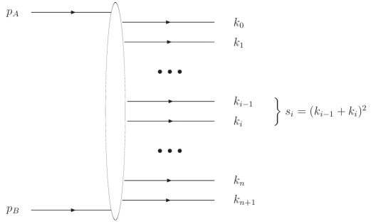
Figure 2.2: Diagrammatic representation of the $s$-channel unitarity relation.

The initial particle momenta $p_{A}$ and $p_{B}$ are assumed to be equal to $p_{A}=p_{1}+(m^{2}_{A}/s)p_{2}$ and $p_{B}=p_{2}+(m^{2}_{B}/s)p_{1}$, respectively. For any momentum $k_{i}$ the Sudakov decomposition is satisfied by the relation

$$k_{i}=\beta_{i}p_{1}+\alpha_{i}p_{2}+k_{i\bot}\;,$$ (2.10)

where $p_{1}$ and $p_{2}$ are light-like vectors and $(p_{1}+p_{2})^{2}=2p_{1}\cdot p_{2}=s$,

$$\alpha_{i}\beta_{i}=\frac{k_{i}^{2}-k_{i\bot}^{2}}{s}=\frac{k_{i}^{2}+\vec{k}_{i}^{2}}{s}\;,$$ (2.11)

with $\vec{k}_{i\bot}$ transverse component with respect to the plane generated by $p_{1}$ and $p_{2}$, and $k_{i\bot}^{2}=-\vec{k}_{i}^{2}$.

The Sudakov decomposition allows us to write the following expression for the phase space:

$$d\Phi_{\tilde{A}\tilde{B}n}=\frac{2}{s}(2\pi)^{D}\delta\left(1+\frac{m_{A}^{2}}{s}-\sum_{i=0}^{n+1}\alpha_{i}\right)\delta\left(1+\frac{m_{B}^{2}}{s}-\sum_{i=0}^{n+1}\beta_{i}\right)$$ (2.12)

$$\times\,\delta^{D-2}\left(\sum_{i=0}^{n+1}k_{i\bot}\right)\frac{d\beta_{n+1}}{2\beta_{n+1}}\frac{d\alpha_{0}}{2\alpha_{0}}\prod_{i=0}^{n}\frac{d\beta_{i}}{2\beta_{i}}\prod_{i=1}^{n+1}\frac{d^{D-2}k_{i\bot}}{(2\pi)^{D-1}}\;,$$

where $p_{\tilde{A}}=k_{0}$ ; $p_{\tilde{B}}=k_{n+1}$. In the unitarity condition (Eq. (2.9)), the dominant contribution ($\sim\!s$) in the LLA is given by the region of limited (not growing with $s$) transverse momenta of produced particles. As we said, large logarithms come from the integration over longitudinal momenta of the produced particles. In particular, we have a logarithm of $s$ for every particle produced according to MRK. By definition, in this kinematics transverse momenta of the produced particles are limited and their Sudakov variables $\alpha_{i}$ and $\beta_{i}$ are strongly ordered in the rapidity space, having so

$$\alpha_{n+1}\gg\alpha_{n}\dots\gg\alpha_{0}\;,$$ (2.13)

$$\beta_{0}\gg\beta_{1}\dots\gg\beta_{n+1}\;.$$

Eqs. (2.10) and (2.13) ensure the squared invariant masses of neighbouring particles,

$$s_{i}=(k_{i-1}+k_{i})^{2}\approx s\beta_{i-1}\alpha_{i}=\frac{\beta_{i-1}}{\beta_{i}}\left(k_{i}^{2}+\vec{k}_{i}^{2}\right)\;,$$ (2.14)

to be large with respect to the squared transverse momenta:

$$s_{i}\gg\vec{k}_{i}^{2}\sim\left|t_{i}\right|=q_{i}^{2}\;,$$ (2.15)

with

$$t_{i}=q_{i}^{2}\approx q_{i\bot}^{2}=-\vec{q}_{i}^{2}$$ (2.16)

and

$$\prod_{i=1}^{n+1}s_{i}=s\prod_{i=1}^{n}\left(k_{i}^{2}+\vec{k}_{i}^{2}\right)\;.$$ (2.17)

In order to obtain the large logarithm from the integration over $\beta_{i}$ for each produced particle in the phase space given in Eq. (2.12), the amplitude in the r.h.s. in Eq. (2.9) must not decrease with the growth of the invariant masses. This is true only when there are exchanges of vector particles (gluons) in all channels with momentum transfers $q_{i=1,\dots,n+1}$ with

$$q_{i}=p_{a}-\sum_{j=0}^{i-1}k_{j}=-\left(p_{B}-\sum_{l=i}^{n+1}k_{l}\right)$$ (2.18)

$$\simeq\beta_{i}p_{1}-\alpha_{i-1}p_{2}-\sum_{j=0}^{i-1}k_{j\bot}$$

and

$$q_{i}^{2}\simeq q_{i\bot}^{2}=-\vec{q}_{i}^{2}$$ (2.19)

The dominant amplitudes at every expansion order can be diagrammatically represented as in Fig. 2.3. Multi-particle amplitudes show a complicated analytical structure even in MRK (see Refs. [Bartels:1974tj, Bartels:1974tk, Bartels:1980pe, Fadin:1993wh]). Fortunately, only real parts of these amplitudes are used in the BFKL approach in NLA as well as in LLA. Considering just the real parts, it is possible to write [Fadin:1998fv]

$$\mathcal{A}^{\tilde{A}\tilde{B}n}_{AB}=2s\Gamma_{\tilde{A}A}^{c_{1}}\left(\prod_{i=1}^{n}\gamma_{c_{i}c_{i+1}}^{P_{i}}(q_{i},q_{i+1})\left(\frac{s_{i}}{s_{R}}\right)^{\omega(t_{i})}\frac{1}{t_{i}}\right)$$ (2.20)

$$\times\,\frac{1}{t_{n+1}}\left(\frac{s_{n+1}}{s_{R}}\right)^{\omega(t_{n+1})}\Gamma_{\tilde{B}B}^{c_{n+1}}$$

with $s_{R}$ being an arbitrary energy scale, irrelevant at LLA. Here $\omega(t)$ and $\Gamma_{P^{\prime}P}^{a}$ are the gluon Regge trajectory and the PPR (see Eq. (2.9)), while $\gamma_{c_{i}c_{i+1}}^{P_{i}}$ are the Reggeon-Reggeon-Particle (RRP) vertices, i.e. the effective vertices for the production of particles $P_{i}$ with momenta $q_{i}-q_{i+1}$ in collisions of Reggeised gluons with momenta $q_{i}$ and $-q_{i+1}$ and colour indices $c_{i}$ and $c_{i+1}$, respectively.

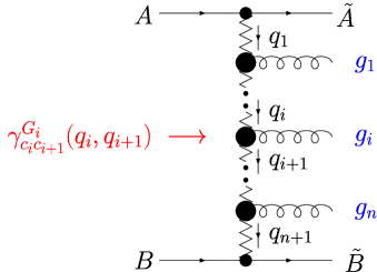
Figure 2.3: Diagrammatic representation of the amplitude $\mathcal{A}^{\tilde{A}\tilde{B}n}_{AB}$.

In the LLA only one gluon can be produced in the RRP vertex. For this reason, final-state particles are massless. The Reggeon-Reggeon-Gluon (RRG) vertex takes the form [BFKL, BFKL_2, BFKL_3, BFKL_4]

$$\gamma_{c_{i}c_{i+1}}^{G_{i}}(q_{i},q_{i+1})=g_{s}T_{c_{i}c_{i+1}}^{d_{i}}e_{\mu}^{\ast}(k_{i})C^{\mu}(q_{i+1},q_{i})\;,$$ (2.21)

where $T_{c_{i}c_{i+1}}^{d_{i}}$ are the matrix elements of the $SU(N_{c})$ group generators in the adjoint representation, $d_{i}$ is the colour index of the produced gluon with polarisation vector $e_{\mu}^{\ast}(k_{i})$, $k_{i}=q_{i}-q_{i+1}$ its momentum and

$$C^{\mu}(q_{i+1},q_{i})=-q_{i}^{\mu}-q_{i+1}^{\mu}+p_{1}^{\mu}\left(\frac{q_{i}^{2}}{k_{i}\cdot p_{1}}+2\frac{k_{i}\cdot p_{2}}{p_{1}\cdot p_{2}}\right)$$ (2.22)

$$\times\,-p_{2}^{\mu}\left(\frac{q_{i+1}^{2}}{k_{i}\cdot p_{2}}+2\frac{k_{i}\cdot p_{1}}{p_{1}\cdot p_{2}}\right)\;.$$

The structure of $C^{\mu}$ given in Eq. (2.22) reflects the current conservation property $(k_{i})_{\mu}C^{\mu}=0$, which permits to choose an arbitrary gauge for each of the produced gluons. Let us introduce now the following decomposition:

$$T_{c_{i}c_{i+1}}^{d_{i}}\left(T_{c_{i}c_{i+1}}^{d_{i}}\right)^{\ast}=\sum_{R}c_{R}\left\langle c_{i}c_{i}^{\prime}\left|\hat{\mathcal{P}}_{R}\right|c_{i+1}c_{i+1}^{\prime}\right\rangle$$ (2.23)

where $\hat{\mathcal{P}}_{R}$ is the projection operator of the two-gluon colour states on the irreducible representation $R$ of the colour group. For the singlet (vacuum) and antisymmetric octet (gluon) representations one has respectively

$$\left\langle c_{i}c_{i}^{\prime}\left|\hat{\mathcal{P}}_{0}\right|c_{i+1}c_{i+1}^{\prime}\right\rangle=\frac{\delta_{c_{i}c_{i}^{\prime}}\delta_{c_{i+1}c_{i+1}^{\prime}}}{N_{c}^{2}-1}$$ (2.24)

and

$$\left\langle c_{i}c_{i}^{\prime}\left|\hat{\mathcal{P}}_{8}\right|c_{i+1}c_{i+1}^{\prime}\right\rangle=\frac{f_{ac_{i}c_{i}^{\prime}}f_{ac_{i+1}c_{i+1}^{\prime}}}{N_{c}}\;,$$ (2.25)

where $f_{abc}$ are the $(SUN_{c})$ structure constants. It is possible to prove that

$$c_{0}=N_{c}\;,\quad\quad c_{8}=\frac{N_{c}}{2}\;.$$ (2.26)

Using the decomposition given in Eq. (2.23), we can write

$$\sum_{G_{i}}\gamma_{c_{i}c_{i+1}}^{G_{i}}(q_{i},q_{i+1})\left(\gamma_{c_{i}c_{i+1}}^{G_{i}}(q_{i},q_{i+1})\right)^{\ast}$$ (2.27)

$$=2(2\pi)^{D-1}\sum_{R}\left\langle c_{i}c_{i}^{\prime}\left|\hat{\mathcal{P}}_{R}\right|c_{i+1}c_{i+1}^{\prime}\right\rangle\mathcal{K}_{r}^{(R)}(\vec{q}_{i},\vec{q}_{i+1};\vec{q})$$

where the sum is taken over colour and polarisation states of the produced gluon and $\mathcal{K}_{r}^{(R)}(\vec{q}_{i},\vec{q}_{i+1};\vec{q})$ is the so-called real part of the kernel.

2.3.1 The BFKL equation

The BFKL equation at LLA is obtained from the amplitude given in Eq. (2.20), using the unitarity relation (see Eq. (2.9)) for the $s$-channel imaginary part of the elastic amplitude, which, according to the decomposition in Eq. (2.23) can be written as

$$\mathcal{A}^{A^{\prime}B^{\prime}}_{AB}=\sum_{R}\left(\mathcal{A}_{R}\right)^{A^{\prime}B^{\prime}}_{AB}\;,$$ (2.28)

where $\left(\mathcal{A}_{R}\right)^{A^{\prime}B^{\prime}}_{AB}$ is the part of the scattering amplitude corresponding to a definite irreducible representation $R$ of the colour group in the $t$-channel. Using the amplitude (2.20) in the unitarity relation (2.9) for the $s$-channel imaginary part of the elastic scattering amplitude, one obtain an expression

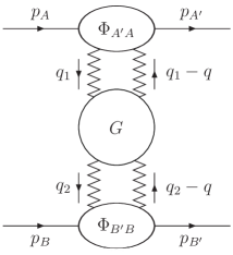
Figure 2.4: Diagrammatic representation of the imaginary part of the BFKL amplitude.

which can be factorised [Fadin:1998sh] in the following way (see Fig. 2.4):

$${\rm Im}\,\left(\mathcal{A}_{R}\right)^{A^{\prime}B^{\prime}}_{AB}=\frac{s}{(2\pi)^{D-2}}\int\frac{d^{D-2}q_{1}}{\vec{q}_{1}^{2}(\vec{q}_{1}-\vec{q})^{2}}\int\frac{d^{D-2}q_{2}}{\vec{q}_{2}^{2}(\vec{q}_{2}-\vec{q})^{2}}$$ (2.29)

$$\times\,\sum_{\nu}\Phi_{A^{\prime}A}^{(R,\nu)}(\vec{q}_{1};\vec{q},s_{0})\int_{\delta-i\infty}^{\delta+i\infty}\frac{d\omega}{2\pi i}\left[\left(\frac{s}{s_{0}}\right)^{\omega}G_{\omega}^{(R)}(\vec{q}_{1},\vec{q}_{2},\vec{q})\right]\Phi_{B^{\prime}B}^{(R,\nu)}(-\vec{q}_{2};-\vec{q},s_{0})\;.$$

Here $\vec{q}_{1}$ and $\vec{q}_{2}$ are the transverse momenta of the Reggeised gluons, while $s_{0}$ is an arbitrary energy scale introduced in order to define the partial wave expansion of the scattering amplitudes via the (inverse) Mellin transform (see Appendix A for further details), while the $\nu$ index identifies the state in the irreducible representation $R$. $\Phi_{P^{\prime}P}^{(R,\nu)}$ are the so-called impact factors, obtained through the convolution of two PPR vertices. $G_{\omega}^{(R)}$, defined via a Mellin transform, is the Green’s function for scattering of two Reggeised gluons and is universal (it does not depend on the particular process). Conversely, the impact factors are specific of the particles on the external lines and can be expressed through the imaginary part of the particle-Reggeon scattering amplitudes, in the form

$$\Phi_{P^{\prime}P}^{(R,\nu)}(\vec{q}_{R};\vec{q};s_{0})=\int\frac{ds_{PR}}{2\pi s}{\rm Im}\,\mathcal{A}_{P^{\prime}P}^{(R,\nu)}(p_{P},q_{R};\vec{q};s_{0})\theta(s_{\Lambda}-s_{PR})$$ (2.30)

$$-\frac{1}{2}\int\frac{d^{D-2}q^{\prime}}{\vec{q}^{\prime 2}(\vec{q}^{\prime}-\vec{q}^{\prime})^{2}}\Phi_{P^{\prime}P}^{(R,\nu)B}(\vec{q}^{\prime},\vec{q})\mathcal{K}_{r}^{(R)B}(\vec{q}^{\prime},\vec{q}_{R})\ln\left(\frac{s_{\Lambda}^{2}}{(\vec{q}^{\prime}-\vec{q}_{R})s_{0}}\right)\;,$$

where $s_{PR}=(q_{P}-q_{R})^{2}$ is the squared particle-Reggeon invariant mass and ${\rm Im}\mathcal{A}_{P^{\prime}}^{(R,\nu)}$ is the $s_{PR}$-channel imaginary part of the scattering amplitude of the particle $P$ with momentum $p_{P}$ off the Reggeon with momentum $q_{R}$, while $q$ is the transferred momentum. This definition is valid both in the LLA and in the NLA. The parameter $s_{\Lambda}$, which plays the role of a cutoff for the $s_{PR}$-integration, is introduced to separate the contributions from MRK and QMRK and must be considered in the limit $s_{\Lambda}\to+\infty$. In this way, the second term in the r.h.s. of Eq. (2.30) works as a counterterm for the large $s_{PR}$.

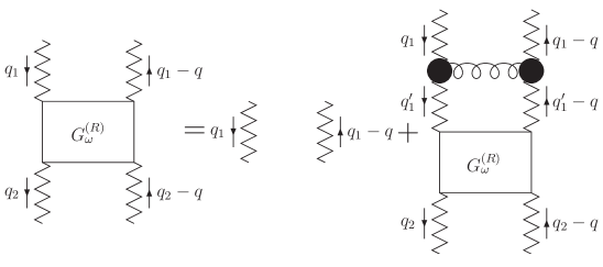
Figure 2.5: Diagrammatic representation of the generalised BFKL integral equation.

The Green’s function obeys the following integral equation (Fig. 2.5), known as generalised BFKL equation:

$$\omega G^{(R)}_{\omega}({\vec{q}}_{1},{\vec{q}}_{2};{\vec{q}})=\vec{q}_{1}^{\leavevmode\nobreak\ 2}({\vec{q}}_{1}-{\vec{q}})^{2}\delta^{(D-2)}({\vec{q}}_{1}-{\vec{q}}_{2})$$ (2.31)

$$+\int\frac{d^{D-2}q_{1\perp}^{\leavevmode\nobreak\ \prime}}{\vec{q}_{1}^{\leavevmode\nobreak\ \prime 2}({\vec{q}}_{1}^{\leavevmode\nobreak\ \prime}-{\vec{q}})^{2}}{\cal K}^{(R)}({\vec{q}}_{1},{\vec{q}}_{1}^{\leavevmode\nobreak\ \prime};{\vec{q}})G^{(R)}_{\omega}({\vec{q}}_{1}^{\leavevmode\nobreak\ \prime},{\vec{q}}_{2};{\vec{q}})\;,$$

where the kernel

$${\cal K}^{(R)}({\vec{q}}_{1},{\vec{q}}_{2};{\vec{q}})=(\omega(q_{1\perp}^{2})+\omega((q_{1}-q)_{\perp}^{2}))\vec{q}_{1}^{\leavevmode\nobreak\ 2}({\vec{q}}_{1}-{\vec{q}})^{2}\delta^{(D-2)}({\vec{q}}_{1}-{\vec{q}}_{2})$$ (2.32)

$$+{\cal K}^{(R)}_{r}({\vec{q}}_{1},{\vec{q}}_{2};{\vec{q}})$$

consists of two parts: the first one is the so-called virtual part and is expressed in terms of the gluon Regge trajectory; the second one, known as real part (see Fig. 2.6), is related to the real particle production and reads:

$${\cal K}_{r}^{(R)}(\vec{q}_{i},\vec{q}_{i+1};\vec{q})=-\frac{g^{2}c_{R}}{2(2\pi)^{D-1}}C^{\mu}(q_{i+1},q_{i})C_{\mu}(q_{i+1}-q,q_{i}-q)$$ (2.33)

$$=\frac{g^{2}c_{R}}{(2\pi)^{D-1}}\left(\frac{{\vec{q}}_{i}^{2}{(\vec{q}_{i+1}-\vec{q})}^{2}+{\vec{q}}_{i+1}^{2}{(\vec{q}_{i}-\vec{q})}^{2}}{({\vec{q}}_{i}-{\vec{q}}_{i+1})^{2}}-\vec{q}^{\leavevmode\nobreak\ 2}\right)\;.$$

If $R=0$ (colour-singlet representation) the Eq. (2.31) is called BFKL equation.

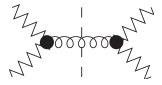
Figure 2.6: Diagrammatic representation of the real part of the BFKL kernel at the Born level.

The BFKL equation iterative: knowing the kernel in the Born level, it permits to get all the LLA terms of the Green’s function. Similarly, knowing all the NLA corrections to the gluon trajectory and to the real part of the kernel, one can get all the NLA terms of the Green’s function. In order to obtain a full amplitude the impact factors are needed, which depend on the process though and have to be calculated time by time at the requested perturbative accuracy. Furthermore, in most cases impact factors encode non-perturbative objects for real processes, e.g. the PDF of the of the parton emitted from the initial state parent hadron and/or the FF describing the detected hadron in the final state within collinear factorisation (in the case of processes with identified particles in the final state). Impact factors are known in the NLA just for few processes.

2.3.2 The BFKL equation in the NLA

Figure 2.7: Diagrammatic representations of replacements $\Gamma_{P^{\prime}P}^{\mathcal{C}({\rm Born})}\to\Gamma_{P^{\prime}P}^{\mathcal{C}(1-{\rm loop})}$ (a) and $\Gamma_{c_{i}c_{i+1}}^{\mathcal{G}_{i}({\rm Born})}\to\Gamma_{c_{i}c_{i+1}}^{\mathcal{G}_{i}(1-{\rm loop})}$ (b).

In order to derive the BFKL equation in the NLA, gluon Reggeisation is assumed to be valid to all orders of perturbation theory. As we said, it has been recently shown that Reggeisation is fulfilled also in the NLA, through the study of the bootstrap conditions [Fadin:2006bj, Kozlov:2011zza, Kozlov:2012zza]. In the NLA, where all terms of the type $\alpha_{s}[\alpha_{s}ln(s)]^{n}$ need be collected, the PPR vertex in Eq. (2.6) assumes the following expression:

$$\Gamma_{P^{\prime}P}=\delta_{\lambda P,\lambda P^{\prime}}\Gamma_{PP}^{(+)}+\delta_{\lambda P^{\prime},-\lambda P}\Gamma_{PP}^{(-)}\;.$$ (2.34)

In this approximation a term in which the helicity of the scattering particle $P$ is not conserved appears. To obtain production amplitudes in the NLA it is sufficient to take one of the vertices or the trajectory in Eq. (2.20) in the NLO. In the LLA, the Reggeised gluon trajectory is needed at 1-loop accuracy and the only contribution to the real part of the kernel is from the production of one gluon at Born level in the collision of two Reggeons ($K_{RRG}^{B}$) [Fadin:1998sh]. In the NLA the gluon trajectory is taken in the NLO (2-loop accuracy [Fadin:1995dd, Fadin:1995km, Kotsky:1996xm, Fadin:1995xg, Fadin:1996tb]) and the real part includes the contributions coming from: one-gluon ($K_{RRG}^{1}$) [Fadin:1992rh], two-gluon ($K_{RRGG}^{B}$) [Fadin:2000kx, Fadin:1996nw, Fadin:1997zv, Kotsky:1998ug], and quark-antiquark pair ($K_{RRQ\bar{Q}}^{B}$) [Fadin:1998jv, Fadin:1997hr, Catani:1990xk, Catani:1990eg] production at Born level [Fadin:1998sh].

Figure 2.8: Diagrammatical representations of replacements $\Gamma_{P^{\prime}P}^{\mathcal{C}({\rm Born})}\to\Gamma_{\{f\}P}^{\mathcal{C}({\rm Born})}$ (a), $\gamma_{c_{i}c_{i+1}}^{\mathcal{G}_{i}({\rm Born})}\to\gamma_{c_{i}c_{i+1}}^{\mathcal{Q\bar{Q}}({\rm Born})}$ (b) and $\gamma_{c_{i}c_{i+1}}^{\mathcal{G}_{i}({\rm Born})}\to\gamma_{c_{i}c_{i+1}}^{\mathcal{GG}({\rm Born})}$ (c) .

The first set of corrections is realised by performing, only in one place, one of the following replacements in the production amplitude (see Eq. (2.20)) entering the $s$-channel unitarity relation:

$$\Gamma_{P^{\prime}P}^{\mathcal{C}({\rm Born})}\to\Gamma_{P^{\prime}P}^{\mathcal{C}(1-{\rm loop})}\;,\quad\quad\gamma_{c_{i}c_{i+1}}^{\mathcal{G}_{i}({\rm Born})}\to\gamma_{c_{i}c_{i+1}}^{\mathcal{G}_{i}(1-{\rm loop})}\;,$$ (2.35)

diagrammatically shown in Fig. 2.7. The second set of corrections consists in allowing the production in the $s$-channel intermediate state of one pair of particles with rapidities of the same order of magnitude, both in the central or in the fragmentation region (QMRK). This implies one replacement among the following in the production amplitude:

$$\Gamma_{P^{\prime}P}^{\mathcal{C}({\rm Born})}\to\Gamma_{\{f\}P}^{\mathcal{C}({\rm Born})}\;,\quad\gamma_{c_{i}c_{i+1}}^{\mathcal{G}_{i}({\rm Born})}\to\gamma_{c_{i}c_{i+1}}^{\mathcal{Q\bar{Q}}({\rm Born})}\;,\quad\gamma_{c_{i}c_{i+1}}^{\mathcal{G}_{i}({\rm Born})}\to\gamma_{c_{i}c_{i+1}}^{\mathcal{GG}({\rm Born})}\;.$$ (2.36)

Here $\Gamma_{\{f\}P}$ stands for the production of a state containing an extra-particle in the fragmentation region of the particle $P$ in the scattering off the Reggeon, $\gamma_{c_{i}c_{i+1}}^{\mathcal{Q\bar{Q}}({\rm Born})}$ and $\gamma_{c_{i}c_{i+1}}^{\mathcal{GG}({\rm Born})}$ are the effective vertices for the production of a quark-antiquark pair and of a two-gluon pair, respectively, in the collision of two Reggeons. This second set of replacements is shown in Fig. 2.8.

2.3.3 The BFKL cross section

The total cross section and many other physical observables are directly related to the imaginary part of the forward scattering amplitude ($\vec{q}=0$) via the optical theorem. The cross section can be expressed by

$$\sigma(s)=\frac{{\rm Im}_{s}\mathcal{A}_{AB}^{AB}}{s}\;,$$ (2.37)

with ${\rm Im}_{s}\mathcal{A}_{AB}^{AB}$ given in Eq. (2.29). It is possible to make the following redefinition of the Green’s function:

$$G_{\omega}(\vec{q}_{1},\vec{q}_{2})=\frac{G^{(0)}_{\omega}({\vec{q}}_{1},{\vec{q}}_{2};0)}{\vec{q}_{1}^{\leavevmode\nobreak\ 2}\vec{q}_{2}^{\leavevmode\nobreak\ 2}}\;,$$ (2.38)

where $\vec{q}_{1,2}$ are two-dimensional vectors and $G^{(0)}_{\omega}({\vec{q}}_{1},{\vec{q}}_{2};0)$ is the forward Green’s function in the singlet-colour representation which obeys the BFKL equation given in Eq. (2.31) with $R=0$. This leads to a simplification of the expressions of the BFKL equation and of the BFKL kernel (2.32), which now read

$$\omega\,G_{\omega}(\vec{q}_{1},\vec{q}_{2})=\delta^{D-2}(\vec{q}_{1}-\vec{q}_{2})+\int d^{D-2}\widetilde{q}\,\,\,{\cal K}(\vec{q}_{1},\vec{\widetilde{q}})\,G_{\omega}(\vec{\widetilde{q}},\vec{q}_{2})\,$$ (2.39)

and

$${\cal K}(\vec{q}_{1},\vec{q}_{2})=\frac{{\cal K}^{(0)}({\vec{q}}_{1},{\vec{q}}_{2};0)}{{\vec{q}}_{1}^{\leavevmode\nobreak\ 2}{\vec{q}}_{2}^{2}}=2\,\omega(-\vec{q}_{1}^{2})\,\delta^{(D-2)}(\vec{q}_{1}-\vec{q}_{2})+{\cal K}_{r}(\vec{q}_{1},\vec{q}_{2})\,,$$ (2.40)

respectively. Here $\omega(-\vec{q}^{\leavevmode\nobreak\ 2})$ is the gluon Regge trajectory given in Eq. (2.8). Due to scale invariance of the kernel, we can take its eigenfunctions as powers of one of the two squared momenta $q_{1,2}^{\leavevmode\nobreak\ 2}$, say $(\vec{q}_{2}^{\leavevmode\nobreak\ 2})^{\gamma-1}$ with $\gamma$ being a complex number. Denoting the corresponding eigenvalues as $\frac{N\alpha_{s}}{\pi}\chi^{B}(\gamma)$, we can write:

$$\int d^{D-2}q_{2}\,\,{\cal K}(\vec{q}_{1},\vec{q}_{2})(\vec{q}_{2}^{\leavevmode\nobreak\ 2})^{\gamma-1}=\frac{N\alpha_{s}}{\pi}\chi^{B}(\gamma)(\vec{q}_{1}^{\leavevmode\nobreak\ 2})^{\gamma-1}\;,$$ (2.41)

with [BFKL, BFKL_2, BFKL_3, BFKL_4]

$$\chi^{B}(\gamma)=2\psi(1)-\psi(\gamma)-\psi(1-\gamma)\,,\,\,\,\psi(\gamma)=\Gamma^{\prime}(\gamma)/\Gamma(\gamma)\,.$$ (2.42)

The set of functions $(\vec{q}_{2}^{\leavevmode\nobreak\ 2})^{\gamma-1}$ with $\gamma=1/2+i\nu,\,\,\,-\infty<\nu<\infty$ is complete and represent the eigenfunctions of the LO BFKL kernel averaged on the azimuthal angle between $\vec{q}_{1}$ and $\vec{q}_{2}$. Taking its projection onto them in Eq. (2.29), one can find the following simple expression for the cross section:

$$\sigma(s)=\frac{1}{(2\pi)^{2}}\int\frac{d^{2}\vec{q}_{1}}{\vec{q}_{1}^{\,\,2}}\Phi_{1}(\vec{q}_{1},s_{0})\int\frac{d^{2}\vec{q}_{2}}{\vec{q}_{2}^{\,\,2}}\Phi_{2}(-\vec{q}_{2},s_{0})$$ (2.43)

$$\times\,\int\limits^{\delta+i\infty}_{\delta-i\infty}\frac{d\omega}{2\pi i}\left(\frac{s}{s_{0}}\right)^{\omega}G_{\omega}(\vec{q}_{1},\vec{q}_{2})\,,$$

which holds with NLA accuracy. All momenta entering this expression are defined on the transverse plane and are therefore two-dimensional. $\Phi_{1,2}$ are the NLO impact factors specific of the process. From this equation it is possible to see that if the Green’s function $G_{\omega}$ has a pole at $\omega^{\prime}$, the cross section at LLA takes the form

$$\sigma^{\rm(LLA)}\sim\frac{s^{\omega_{P}^{B}}}{\sqrt{\ln s}}\;,\quad\omega^{\prime}\equiv\omega_{P}^{B}\;,$$ (2.44)

where $\omega_{P}^{B}$ is the $(t=0)$-intercept of the Regge trajectory that rules the asymptotic behaviour in $s$ of the amplitude with exchange of the vacuum quantum numbers in the $t$-channel. It is equal to $4N_{c}(\alpha_{s}/\pi)\ln 2$, which implies violation of the Froissart bound [Froissart:1961ux], giving rise to a power-like behaviour of cross section with energy. The BFKL unitarity restoration is an open issue, which goes beyond the scope of this thesis. We mention here some of the solution methods proposed so far: the Balitsky–Kovchegov (BK) scheme [Balitsky:1995ub, Kovchegov:1999yj], which generalises the BFKL evolution equation (2.31) through the inclusion of non-linear terms that tame the growth of the cross section; the Bartels–Kwiecinski–Praszalowicz (BKP) method [Bartels:1980pe, Kwiecinski:1980wb], which introduces composite states of several Reggeised gluons; approaches based on gauge-invariant effective field theories for the Reggeised gluon interactions [Lipatov:1995pn, Lipatov:1996ts].

Besides the unitarity issue, there is another important question that should be contemplated, i.e. whether the characteristic growth with energy of sufficiently inclusive cross sections, which represents the most striking prediction of the BFKL Pomeron, could be observed in actual and forthcoming LHC analyses. This possibility will be examined in the course of our study on inclusive dijet production (see Section 3.6).

As we saw in Section 2.3.1, the Green’s function $G_{\omega}$ takes care of the universal, energy-dependent part of the amplitude and obeys the BFKL equation (2.31).

In this section we derive a general form for the cross section in the so-called $(\nu,n)$-representation (for more details, see Refs. [Ivanov:2005gn, Ivanov:2006gt]), which will provide us with the starting point of our further analysis. First of all, it is convenient to work in the transverse momentum representation, defined by

$$\hat{\vec{q}}\>|\vec{q}_{i}\rangle=\vec{q}_{i}|\vec{q}_{i}\rangle\;,\quad\quad\langle\vec{q}_{1}|\vec{q}_{2}\rangle=\delta^{(2)}(\vec{q}_{1}-\vec{q}_{2})\;,$$ (2.45)

$$\langle A|B\rangle=\langle A|\vec{k}\rangle\langle\vec{k}|B\rangle=\int d^{2}kA(\vec{k})B(\vec{k})\;.$$

In this representation, the total cross section given in Eq. (2.43) takes the simple form

$$\sigma=\frac{1}{(2\pi)^{2}}\int_{\delta-i\infty}^{\delta+i\infty}\frac{d\omega}{2\pi i}\,\left(\frac{s}{s_{0}}\right)^{\omega}\langle\frac{\Phi_{1}}{\vec{q}_{1}^{\,\,2}}|\hat{G}_{\omega}|\frac{\Phi_{2}}{\vec{q}_{2}^{\,\,2}}\rangle\ .$$ (2.46)

The kernel of the operator $\hat{K}$ becomes

$$K(\vec{q}_{2},\vec{q}_{1})=\langle\vec{q}_{2}|\hat{K}|\vec{q}_{1}\rangle$$ (2.47)

and the equation for the Green’s function reads

$$\hat{1}=(\omega-\hat{K})\hat{G}_{\omega}\;,$$ (2.48)

its solution being

$$\hat{G}_{\omega}=(\omega-\hat{K})^{-1}\,.$$ (2.49)

The kernel is given as an expansion in the strong coupling,

$$\hat{K}=\bar{\alpha}_{s}\hat{K}^{0}+\bar{\alpha}_{s}^{2}\hat{K}^{1}\;,$$ (2.50)

where

$${\bar{\alpha}_{s}}\equiv\frac{N_{c}}{\pi}\alpha_{s}$$ (2.51)

and $N_{c}$ is the number of colours. In Eq. (2.50) $\hat{K}^{0}$ is the BFKL kernel in the leading order (LO), while $\hat{K}^{1}$ represents the NLO correction.

To determine the cross section with NLA accuracy we need an approximate solution of Eq. (2.49). With the required accuracy this solution is

$$\hat{G}_{\omega}=(\omega-\bar{\alpha}_{s}\hat{K}^{0})^{-1}$$ (2.52)

$$+(\omega-\bar{\alpha}_{s}\hat{K}^{0})^{-1}\left(\bar{\alpha}_{s}^{2}\hat{K}^{1}\right)(\omega-\bar{\alpha}_{s}\hat{K}^{0})^{-1}+{\cal O}\left[\left(\bar{\alpha}_{s}^{2}\hat{K}^{1}\right)^{2}\right]\,.$$

In Eq. (2.41) we gave the expressions for the eigenfunctions of the LO kernel averaged on the azimuthal angle. In the general case the basis of eigenfunctions of the LO kernel,

$$\hat{K}^{0}|n,\nu\rangle=\chi(n,\nu)|n,\nu\rangle\,,$$ (2.53)

$$\chi(n,\nu)=2\psi(1)-\psi\left(\frac{n}{2}+\frac{1}{2}+i\nu\right)-\psi\left(\frac{n}{2}+\frac{1}{2}-i\nu\right)\,,$$

is given by the following set of functions:

$$\langle\vec{q}\,|n,\nu\rangle=\frac{1}{\pi\sqrt{2}}\left(\vec{q}^{\,\,2}\right)^{i\nu-\frac{1}{2}}e^{in\phi}\;,$$ (2.54)

which now depend not only on $\nu$, but also on the integer $n$, called conformal spin. Here $\phi$ is the azimuthal angle of the vector $\vec{q}$ counted from some fixed direction in the transverse space, $\cos\phi\equiv q_{x}/|\vec{q}\,|$. Then, the orthonormality and completeness conditions take the form

$$\langle n^{\prime},\nu^{\prime}|n,\nu\rangle=\int\frac{d^{2}\vec{q}}{2\pi^{2}}\left(\vec{q}^{\,\,2}\right)^{i\nu-i\nu^{\prime}-1}e^{i(n-n^{\prime})\phi}=\delta(\nu-\nu^{\prime})\,\delta_{nn^{\prime}}$$ (2.55)

and

$$\hat{1}=\sum^{\infty}_{n=-\infty}\int\limits^{\infty}_{-\infty}d\nu\,|n,\nu\rangle\langle n,\nu|\ .$$ (2.56)

The action of the full NLO BFKL kernel on these functions may be expressed as follows:

$$\hat{K}|n,\nu\rangle=\bar{\alpha}_{s}(\mu_{R})\chi(n,\nu)|n,\nu\rangle$$ (2.57)

$$+\bar{\alpha}_{s}^{2}(\mu_{R})\left(\chi^{(1)}(n,\nu)+\frac{\beta_{0}}{4N_{c}}\chi(n,\nu)\ln(\mu^{2}_{R})\right)|n,\nu\rangle$$

$$+\bar{\alpha}_{s}^{2}(\mu_{R})\frac{\beta_{0}}{4N_{c}}\chi(n,\nu)\left(i\frac{\partial}{\partial\nu}\right)|n,\nu\rangle\;,$$

where $\mu_{R}$ is the renormalisation scale of the QCD coupling; the first term represents the action of LO kernel, while the second and the third ones stand for the diagonal and the non-diagonal parts of the NLO kernel and we have used

$$\beta_{0}=\frac{11N_{c}}{3}-\frac{2n_{f}}{3}\;,$$ (2.58)

where $n_{f}$ is the number of active quark flavours.

The function $\chi^{(1)}(n,\nu)$, calculated in Ref. [Kotikov:2000pm] (see also Ref. [Kotikov:2002ab]), is conveniently represented in the form

$$\chi^{(1)}(n,\nu)=-\frac{\beta_{0}}{8\,N_{c}}\left(\chi^{2}(n,\nu)-\frac{10}{3}\chi(n,\nu)-i\chi^{\prime}(n,\nu)\right)+{\bar{\chi}}(n,\nu)\,,$$ (2.59)

where

$$\bar{\chi}(n,\nu)\,=\,-\frac{1}{4}\left[\frac{\pi^{2}-4}{3}\chi(n,\nu)-6\zeta(3)-\chi^{\prime\prime}(n,\nu)+\,2\,\phi(n,\nu)\right.$$ (2.60)

$$+\,2\,\phi(n,-\nu)+\frac{\pi^{2}\sinh(\pi\nu)}{2\,\nu\,\cosh^{2}(\pi\nu)}\left(\left(3+\left(1+\frac{n_{f}}{N_{c}^{3}}\right)\frac{11+12\nu^{2}}{16(1+\nu^{2})}\right)\delta_{n0}\right.$$

$$\left.\left.-\left(1+\frac{n_{f}}{N_{c}^{3}}\right)\frac{1+4\nu^{2}}{32(1+\nu^{2})}\delta_{n2}\right)\right]\,,$$

and

$$\phi(n,\nu)\,=\,-\int\limits_{0}^{1}dx\,\frac{x^{-1/2+i\nu+n/2}}{1+x}\left[\frac{1}{2}\left(\psi^{\prime}\left(\frac{n+1}{2}\right)-\zeta(2)\right)\right.$$ (2.61)

$$+\mbox{Li}_{2}(x)+\mbox{Li}_{2}(-x)+\ln x\left(\psi(n+1)-\psi(1)+\ln(1+x)+\sum_{k=1}^{\infty}\frac{(-x)^{k}}{k+n}\right)$$

$$\left.+\sum_{k=1}^{\infty}\frac{x^{k}}{(k+n)^{2}}(1-(-1)^{k})\right]$$

$$=\sum_{k=0}^{\infty}\frac{(-1)^{k+1}}{k+(n+1)/2+i\nu}\left[\psi^{\prime}(k+n+1)-\psi^{\prime}(k+1)\right.$$

$$+(-1)^{k+1}(\beta^{\prime}(k+n+1)+\beta^{\prime}(k+1))$$

$$\left.-\frac{1}{k+(n+1)/2+i\nu}(\psi(k+n+1)-\psi(k+1))\right]\;,$$

$$\beta^{\prime}(z)=\frac{1}{4}\left[\psi^{\prime}\left(\frac{z+1}{2}\right)-\psi^{\prime}\left(\frac{z}{2}\right)\right]\;,$$ (2.62)

$$\mbox{Li}_{2}(x)=-\int\limits_{0}^{x}dt\,\frac{\ln(1-t)}{t}\;.$$ (2.63)

Here and below $\chi^{\prime}(n,\nu)\equiv d\chi(n,\nu)/d\nu$ and $\chi^{\prime\prime}(n,\nu)\equiv d^{2}\chi(n,\nu)/d^{2}\nu$.

The projection of the impact factors onto the eigenfunctions of the LO BFKL kernel, i.e. the transfer to the $(\nu,n)$-representation, is done as follows:

$$\frac{\Phi_{1}(\vec{q}_{1})}{\vec{q}_{1}^{\,\,2}}=\sum^{+\infty}_{n=-\infty}\int\limits^{+\infty}_{-\infty}d\nu\,\Phi_{1}(\nu,n)\langle n,\nu|\vec{q}_{1}\rangle\,\;,$$ (2.64)

$$\frac{\Phi_{2}(-\vec{q_{2}})}{\vec{q}_{2}^{\,\,2}}=\sum^{+\infty}_{n=-\infty}\int\limits^{+\infty}_{-\infty}d\nu\,\Phi_{2}(\nu,n)\langle\vec{q}_{2}|n,\nu\rangle\;,$$

$$\Phi_{1}(\nu,n)=\langle\frac{\Phi_{1}(\vec{q}_{1})}{\vec{q}_{1}^{\,\,2}}|n,\nu\rangle\equiv\int d^{2}q_{1}\,\frac{\Phi_{1}(\vec{q}_{1})}{\vec{q}_{1}^{\,\,2}}\frac{1}{\pi\sqrt{2}}\left(\vec{q}_{1}^{\,\,2}\right)^{i\nu-\frac{1}{2}}e^{in\phi_{1}}\;,$$ (2.65)

$$\Phi_{2}(\nu,n)=\langle n,\nu|\frac{\Phi_{2}(-\vec{q}_{2})}{\vec{q}_{2}^{\,\,2}}\rangle\equiv\int d^{2}q_{2}\,\frac{\Phi_{2}(-\vec{q}_{2})}{\vec{q}_{2}^{\,\,2}}\frac{1}{\pi\sqrt{2}}\left(\vec{q}_{2}^{\,\,2}\right)^{-i\nu-\frac{1}{2}}e^{-in\phi_{2}}\;.$$

The impact factors can be represented as an expansion in $\alpha_{s}$,

$$\Phi_{1,2}(\vec{q}\,)=\alpha_{s}(\mu_{R})\left[v_{1,2}(\vec{q}\,)+\bar{\alpha}_{s}(\mu_{R})v_{1,2}^{(1)}(\vec{q}\,)\right]$$ (2.66)

and

$$\Phi_{1,2}(n,\nu)=\alpha_{s}(\mu_{R})\left[c_{1,2}(n,\nu)+\bar{\alpha}_{s}(\mu_{R})c_{1,2}^{(1)}(n,\nu)\right]\,.$$ (2.67)

To obtain our representation of the cross section, the matrix element of the BFKL Green’s function is needed. According to Eq. (2.52), one has

$$\langle n,\nu|\hat{G}_{\omega}|n^{\prime},\nu^{\prime}\rangle=\delta_{n,n^{\prime}}\left[\delta(\nu-\nu^{\prime})\left(\frac{1}{\omega-\bar{\alpha}_{s}(\mu_{R})\chi(n,\nu)}\right.\right.$$ (2.68)

$$\left.+\frac{1}{(\omega-\bar{\alpha}_{s}(\mu_{R})\chi(n,\nu))^{2}}\left(\bar{\alpha}_{s}^{2}(\mu_{R})(\bar{\chi}(n,\nu)\right.\right.$$

$$\left.\left.+\frac{\beta_{0}}{8N_{c}}(-\chi^{2}(n,\nu)+\frac{10}{3}\chi(n,\nu)+2\chi(n,\nu)\ln\mu_{R}^{2}+i\frac{d}{d\nu}\chi(n,\nu)))\right)\right)$$

$$\left.+\frac{\frac{\beta_{0}}{4N_{c}}\bar{\alpha}_{s}^{2}(\mu_{R})\chi(n,\nu^{\prime})}{(\omega-\bar{\alpha}_{s}(\mu_{R})\chi(n,\nu))(\omega-\bar{\alpha}_{s}(\mu_{R})\chi(n,\nu^{\prime}))}\left(i\frac{d}{d\nu^{\prime}}\delta(\nu-\nu^{\prime})\right)\right]\ .$$

Inserting twice the unity operator, written according to the completeness condition given in Eq. (2.56), into Eq. (2.46), we get

$$\sigma=\frac{1}{(2\pi)^{2}}\sum^{\infty}_{n=-\infty}\int\limits^{\infty}_{-\infty}d\nu\sum^{\infty}_{n^{\prime}=-\infty}\int\limits^{\infty}_{-\infty}d\nu^{\prime}\int_{\delta-i\infty}^{\delta+i\infty}\frac{d\omega}{2\pi i}\left(\frac{1}{s_{0}}\right)^{\omega}$$ (2.69)

$$\langle\frac{\Phi_{1}}{\vec{q}_{1}^{\,\,2}}|n,\nu\rangle\langle n,\nu|\hat{G}_{\omega}|n^{\prime},\nu^{\prime}\rangle\langle n^{\prime},\nu^{\prime}|\frac{\Phi_{2}}{\vec{q}_{2}^{\,\,2}}\rangle\ ,$$

and, after some algebra and integration by parts, finally

$$\sigma=\frac{1}{(2\pi)^{2}}\sum^{\infty}_{n=-\infty}\int\limits^{\infty}_{-\infty}d\nu\left(\frac{s}{s_{0}}\right)^{\bar{\alpha}_{s}(\mu_{R})\chi(n,\nu)}$$ (2.70)

$$\alpha_{s}^{2}(\mu_{R})c_{1}(n,\nu)c_{2}(n,\nu)\left[1+\bar{\alpha}_{s}(\mu_{R})\left(\frac{c^{(1)}_{1}(n,\nu)}{c_{1}(n,\nu)}+\frac{c^{(1)}_{2}(n,\nu)}{c_{2}(n,\nu)}\right)\right.$$

$$+\bar{\alpha}^{2}_{s}(\mu_{R})\ln\frac{s}{s_{0}}\left\{\bar{\chi}(n,\nu)+\frac{\beta_{0}}{8N_{c}}\chi(n,\nu)\right.$$

$$\left.\left.\left(-\chi(n,\nu)+\frac{10}{3}+2\ln\mu_{R}^{2}+i\frac{d}{d\nu}\ln\frac{c_{1}(n,\nu)}{c_{2}(n,\nu)}\right)\right\}\right]\,.$$

In order to assess the relative weight of NLA corrections with respect to the LLA contribution, one can confront $\chi^{(1)}(n,\nu)$ (Eq. (2.59)) with $\chi(n,\nu)$ (Eq. (2.53)) for $n=0$ and $\nu=0$, i.e. for the point in the $(\nu,n)$-space which determines the energy asymptotic behaviour in the LLA case. The result found for the ratio $|\chi^{(1)}(0,0)/\chi(0,0)|$ is large ($\simeq 6.5$) [Fadin:1998py, Ciafaloni:1998gs], thus leading to instabilities in the BFKL perturbative expansion, which have to be controlled through some optimisation procedure. In Section 2.4 we will discuss one of them, which represent perhaps the most effetive tool to quench the oscillating behaviour of the BFKL series.

2.3.3.1 Representation equivalence

The expression for the cross section given in Eq. (2.70) is valid both in the LLA and in the NLA. However, it is not the only possible one. Actually, several NLA-equivalent expressions can be adopted. One can consider alternative representations aiming at catching some of the unknown next-to-NLA corrections. Here we show two examples, which have been used in recent phenomenological analyses (for more details, see Ref. [Caporale:2014gpa]):

• the so-called exponentiated representation,

  $$\sigma^{\rm exp}=\frac{1}{(2\pi)^{2}}\sum^{\infty}_{n=-\infty}\int\limits^{\infty}_{-\infty}d\nu\,\alpha_{s}^{2}(\mu_{R})c_{1}(n,\nu)c_{2}(n,\nu)$$ (2.71)

  $$\times\,\left(\frac{s}{s_{0}}\right)^{\bar{\alpha}_{s}(\mu_{R})\chi+\bar{\alpha}^{2}_{s}(\mu_{R})\left\{\bar{\chi}+\frac{\beta_{0}}{8N_{c}}\chi\left(-\chi+\frac{10}{3}+2\ln\mu_{R}^{2}+i\frac{d}{d\nu}\ln\frac{c_{1}(n,\nu)}{c_{2}(n,\nu)}\right)\right\}}$$

  $$\times\,\left[1+\bar{\alpha}_{s}(\mu_{R})\left(\frac{c^{(1)}_{1}(n,\nu)}{c_{1}(n,\nu)}+\frac{c^{(1)}_{2}(n,\nu)}{c_{2}(n,\nu)}\right)\right]\;;$$

• the exponentiated representation with an extra, irrelevant in the NLA term, given by the product of the NLO corrections of the two impact factors,

  $$\sigma^{\rm exp\,(c)}=\frac{1}{(2\pi)^{2}}\sum^{\infty}_{n=-\infty}\int\limits^{\infty}_{-\infty}d\nu\,\alpha_{s}^{2}(\mu_{R})c_{1}(n,\nu)c_{2}(n,\nu)$$ (2.72)

  $$\times\,\left(\frac{s}{s_{0}}\right)^{\bar{\alpha}_{s}(\mu_{R})\chi+\bar{\alpha}^{2}_{s}(\mu_{R})\left\{\bar{\chi}+\frac{\beta_{0}}{8N_{c}}\chi\left(-\chi+\frac{10}{3}+2\ln\mu_{R}^{2}+i\frac{d}{d\nu}\ln\frac{c_{1}(n,\nu)}{c_{2}(n,\nu)}\right)\right\}}$$

  $$\times\,\left[1+\bar{\alpha}_{s}(\mu_{R})\left(\frac{c^{(1)}_{1}(n,\nu)}{c_{1}(n,\nu)}+\frac{c^{(1)}_{2}(n,\nu)}{c_{2}(n,\nu)}\right)\right.$$

  $$\left.+\,\alpha_{s}^{2}\left(\mu_{R}\right)\left(\frac{c_{1}^{\left(1\right)}\left(n,\nu\right)}{c_{1}\left(n,\nu\right)}\frac{c_{2}^{\left(1\right)}\left(n,\nu\right)}{c_{2}\left(n,\nu\right)}\right)\right]\;.$$

In Eqs. (2.71) and (2.72) is the LO kernel eigenvalue given in (2.53). In our calculations for Mueller–Navelet jet (see Chapter 3) and dihadron (see Chapter 3) production processes, we will adopt the exponentiated representation (Eq. (2.71)).

2.4 The BLM optimisation procedure

It is well known that the BFKL approach is plagued by large NLA corrections (see the discussion at the end of Section 2.3.3), both in the kernel of the Green’s function and in the process-dependent impact factors, as well as by large uncertainties in the renormalisation scale setting. As an example, the NLA BFKL corrections for the $n=0$ conformal spin are with opposite sign with respect to the LLA results and large in absolute value. All that calls for some optimisation procedure of the perturbative series, which can consist in (i) including some pieces of the (unknown) next-to-NLA corrections, such as those dictated by renormalisation group, as in collinear improvement [Caporale:2013uva, Vera:2007kn, Salam:1998tj, Ciafaloni:1998iv, Ciafaloni:1999yw, Ciafaloni:1999au, Ciafaloni:2000cb, Ciafaloni:2002xk, Ciafaloni:2002xf, Ciafaloni:2003ek, Ciafaloni:2003rd, Ciafaloni:2003kd, Vera:2005jt, Caporale:2007vs], or by energy-momentum conservation [Kwiecinski:1999yx], or (ii) suppressing the emission of gluons which are close by in rapidity in the BFKL framework (rapidity veto approach [Schmidt:1999mz, Forshaw:1999xm]), and/or (iii) suitably choosing the values of the energy and renormalisation scales, which, though arbitrary within the NLO, can have a sizeable numerical impact through subleading terms. Common optimisation methods are those inspired by the principle of minimum sensitivity (PMS) [PMS, PMS_2], the fast apparent convergence (FAC) [FAC, FAC_2, FAC_3] and the Brodsky–Lepage–Mackenzie method (BLM) [BLM, BLM_2, BLM_3, BLM_4, BLM_5].

In this Section we present and discuss the widely-used BLM approach, which relies on the removal of the renormalisation scale ambiguity by absorbing the non-conformal $\beta_{0}$-terms into the running coupling. It is known that after BLM scale setting, the QCD perturbative convergence can be greatly improved due to the elimination of renormalon terms in the perturbative QCD series. Moreover, with the BLM scale setting, the BFKL Pomeron intercept has a weak dependence on the virtuality of the Reggeised gluon [BLM_4, BLM_5].

We provide, as result, an exact implementation of the BLM method, together with two other, approximated ones, which were used earlier in the literature of the BLM method for different semi-hard processes (see a more detailed discussion in [Caporale:2015uva]).

We consider the BLM scale setting for the separate contributions to the cross section, specified in Eq. (2.70) by different values of $n$, denoted in the following by ${\cal C}_{n}$. The starting point of our considerations is the expression for ${\cal C}_{n}$ in the $\overline{\rm MS}$ scheme (see Eq. (2.70)),

$${\cal C}_{n}=\frac{1}{(2\pi)^{2}}\int\limits^{\infty}_{-\infty}d\nu\left(\frac{s}{s_{0}}\right)^{\bar{\alpha}_{s}(\mu_{R})\chi(n,\nu)}\alpha_{s}^{2}(\mu_{R})c_{1}(n,\nu)c_{2}(n,\nu)$$ (2.73)

$$\times\,\left[1+\bar{\alpha}_{s}(\mu_{R})\left(\frac{c^{(1)}_{1}(n,\nu)}{c_{1}(n,\nu)}+\frac{c^{(1)}_{2}(n,\nu)}{c_{2}(n,\nu)}\right)\right.$$

$$+\,\bar{\alpha}^{2}_{s}(\mu_{R})\ln\frac{s}{s_{0}}\left\{\bar{\chi}(n,\nu)+\frac{\beta_{0}}{8N_{c}}\chi(n,\nu)\right.$$

$$\times\,\left.\left.\left(-\chi(n,\nu)+\frac{10}{3}+2\ln\mu_{R}^{2}+i\frac{d}{d\nu}\ln\frac{c_{1}(n,\nu)}{c_{2}(n,\nu)}\right)\right\}\right]\,.$$

In the r.h.s. of this expression we have terms $\sim\alpha_{s}$ originated from the NLO corrections to the impact factors, and terms $\sim\alpha^{2}_{s}\ln(s/s_{0})$ coming from NLA corrections to the BFKL kernel. In the latter case, the terms proportional to the QCD $\beta$-function are explicitly shown. For our further consideration of the BLM scale setting, similar contributions have to be separated also from the NLO impact factors.

In fact, the contribution to an NLO impact factor that is proportional to $\beta_{0}$ is universally expressed through the LO impact factor,

$$v^{(1)}(\vec{q}\,)=v(\vec{q}\,)\frac{\beta_{0}}{4N_{c}}\left(\ln\left(\frac{\mu_{R}^{2}}{\vec{q}\,^{2}}\right)+\frac{5}{3}\right)+\dots\ ,$$ (2.74)

where the dots stand for the other terms, not proportional to $\beta_{0}$. This statement becomes evident if one considers the part of the strong coupling renormalisation proportional to $n_{f}$ and related to the contributions of light quark flavours. Such contribution to the NLO impact factor originates only from diagrams with the light quark loop insertion in the Reggeised gluon propagator. The results for such contributions can be found, for instance, in Eq. (5.1) of [Fadin:2001ap]. Tracing there the terms $\sim n_{f}$ and performing the QCD charge renormalisation, one can indeed confirm (Eq. (2.74)).

Transforming Eq. (2.74) to the $\nu$-representation according to Eq. (2.65), we obtain

$${\tilde{c}}_{1}^{\left(1\right)}(\nu,n) = \frac{\beta_{0}}{4N_{c}}\left[+i\frac{d}{d\nu}c_{1}(\nu,n)+\left(\ln\mu_{R}^{2}+\frac{5}{3}\right)c_{1}(\nu,n)\right]\ ,$$

$${\tilde{c}}_{2}^{\left(1\right)}(\nu,n) = \frac{\beta_{0}}{4N_{c}}\left[-i\frac{d}{d\nu}c_{2}(\nu,n)+\left(\ln\mu_{R}^{2}+\frac{5}{3}\right)c_{2}(\nu,n)\right]\ ,$$ (2.75)

and

$$\frac{{\tilde{c}}_{1}^{\left(1\right)}}{c_{1}}+\frac{{\tilde{c}}_{2}^{\left(1\right)}}{c_{2}}=\frac{\beta_{0}}{4N_{c}}\left[i\frac{d}{d\nu}\ln\left(\frac{c_{1}}{c_{2}}\right)+2\left(\ln\mu_{R}^{2}+\frac{5}{3}\right)\right]\ .$$ (2.76)

It is convenient to introduce the function $f\left(\nu\right)$, defined through

$$i\frac{d}{d\nu}\ln\left(\frac{c_{1}}{c_{2}}\right)\equiv 2\left[f(\nu)-\ln\left(Q_{1}Q_{2}\right)\right]\ ,$$ (2.77)

that depends on the given process, where $Q_{1,2}$ denote here the hard scales which enter the impact factors $c_{1,2}$. The specific form of the function $f(\nu)$ depends on the particular process.

Now, we present again our result for the generic observable ${\cal C}_{n}$, showing explicitly all contributions proportional to the QCD $\beta$-function, i.e. also those originating from the impact factors:

$${\cal C}_{n}=\frac{1}{(2\pi)^{2}}\int\limits^{\infty}_{-\infty}d\nu\left(\frac{s}{s_{0}}\right)^{\bar{\alpha}_{s}(\mu_{R})\chi(n,\nu)}\alpha_{s}^{2}(\mu_{R})c_{1}(n,\nu)c_{2}(n,\nu)$$ (2.78)

$$\times\,\left[1+\bar{\alpha}_{s}(\mu_{R})\left(\frac{\bar{c}^{(1)}_{1}(n,\nu)}{c_{1}(n,\nu)}+\frac{\bar{c}^{(1)}_{2}(n,\nu)}{c_{2}(n,\nu)}+\frac{\beta_{0}}{2N_{c}}\left(\frac{5}{3}+\ln\frac{\mu_{R}^{2}}{Q_{1}Q_{2}}+f(\nu)\right)\right)\right.$$

$$\left.+\,\bar{\alpha}^{2}_{s}(\mu_{R})\ln\frac{s}{s_{0}}\left\{\bar{\chi}(n,\nu)+\frac{\beta_{0}}{4N_{c}}\chi(n,\nu)\left(-\frac{\chi(n,\nu)}{2}+\frac{5}{3}+\ln\frac{\mu_{R}^{2}}{Q_{1}Q_{2}}+f(\nu)\right)\right\}\right]\,,$$

where $\bar{c}^{(1)}_{1,2}\equiv c^{(1)}_{1,2}-\tilde{c}^{(1)}_{1,2}$. We note that the dependence of Eq. (2.78) on the scale $\mu_{R}$ is subleading: performing in Eq. (2.78) the replacement

$$\alpha_{s}(\mu_{R})=\alpha_{s}(\mu^{\prime}_{R})\left(1-\bar{\alpha}_{s}(\mu^{\prime}_{R})\frac{\beta_{0}}{2N_{c}}\ln\frac{\mu_{R}}{\mu^{\prime}_{R}}\right)\,,$$ (2.79)

one indeed obtains the same expression as before with the new scale $\mu_{R}^{\prime}$ at the place of the old one $\mu_{R}$, plus some additional contributions which are beyond the NLA accuracy.

As the next step, we perform a finite renormalisation from the $\overline{\rm MS}$ to the physical MOM scheme, that means:

$$\alpha_{s}^{\overline{\rm MS}}=\alpha_{s}^{\rm MOM}\left(1+\frac{\alpha_{s}^{\rm MOM}}{\pi}T\right)\;,$$ (2.80)

with

$$T=T^{\beta}+T^{\rm conf}\;,$$ (2.81)

$$T^{\beta}=-\frac{\beta_{0}}{2}\left(1+\frac{2}{3}I\right)\;,$$

$$T^{\rm conf}=\frac{C_{A}}{8}\left[\frac{17}{2}I+\frac{3}{2}\left(I-1\right)\xi+\left(1-\frac{1}{3}I\right)\xi^{2}-\frac{1}{6}\xi^{3}\right]\;,$$

where $C_{A}\equiv N_{c}$ is the colour factor associated with gluon emission from a gluon, $I=-2\int_{0}^{1}dx\frac{\ln\left(x\right)}{x^{2}-x+1}\simeq 2.3439$ and $\xi$ is a gauge parameter, fixed at zero in the following.

Inserting Eq. (2.80) into Eq. (2.78) and expanding the result, we obtain, within NLA accuracy,

$${\cal C}^{\rm MOM}_{n}=\frac{1}{(2\pi)^{2}}\int\limits^{\infty}_{-\infty}d\nu\left(\frac{s}{s_{0}}\right)^{\bar{\alpha}^{\rm MOM}_{s}(\mu_{R})\chi(n,\nu)}\left(\alpha^{\rm MOM}_{s}(\mu_{R})\right)^{2}$$ (2.82)

$$\times\,c_{1}(n,\nu)c_{2}(n,\nu)\left[1+\bar{\alpha}^{\rm MOM}_{s}(\mu_{R})\left\{\frac{\bar{c}^{(1)}_{1}(n,\nu)}{c_{1}(n,\nu)}+\frac{\bar{c}^{(1)}_{2}(n,\nu)}{c_{2}(n,\nu)}+\frac{2T^{\rm conf}}{N_{c}}\right.\right.$$

$$\left.+\,\frac{\beta_{0}}{2N_{c}}\left(\frac{5}{3}+\ln\frac{\mu_{R}^{2}}{Q_{1}Q_{2}}+f(\nu)-2\left(1+\frac{2}{3}I\right)\right)\right\}$$

$$+\,\left(\bar{\alpha}^{\rm MOM}_{s}(\mu_{R})\right)^{2}\ln\frac{s}{s_{0}}\left\{\bar{\chi}(n,\nu)+\frac{T^{\rm conf}}{N_{c}}\chi(n,\nu)\right.$$

$$\left.\left.+\,\frac{\beta_{0}}{4N_{c}}\chi(n,\nu)\left(-\frac{\chi(n,\nu)}{2}+\frac{5}{3}+\ln\frac{\mu_{R}^{2}}{Q_{1}Q_{2}}+f(\nu)-2\left(1+\frac{2}{3}I\right)\right)\right\}\right]\,.$$

The optimal scale $\mu_{R}^{\rm BLM}$ is the value of $\mu_{R}$ that makes the expression proportional to $\beta_{0}$ vanish. We thus have

$${\cal C}^{\beta}_{n}=\frac{1}{(2\pi)^{2}}\int\limits^{\infty}_{-\infty}d\nu\left(\frac{s}{s_{0}}\right)^{\bar{\alpha}^{\rm MOM}_{s}(\mu^{\rm BLM}_{R})\chi(n,\nu)}\left(\alpha^{\rm MOM}_{s}(\mu^{\rm BLM}_{R})\right)^{3}$$ (2.83)

$$\times\,c_{1}(n,\nu)c_{2}(n,\nu)\frac{\beta_{0}}{2N_{c}}\left[\frac{5}{3}+\ln\frac{(\mu^{\rm BLM}_{R})^{2}}{Q_{1}Q_{2}}+f(\nu)-2\left(1+\frac{2}{3}I\right)\right.$$

$$+\,\bar{\alpha}^{\rm MOM}_{s}(\mu^{\rm BLM}_{R})\ln\frac{s}{s_{0}}\>\frac{\chi(n,\nu)}{2}$$

$$\times\,\left.\left(-\frac{\chi(n,\nu)}{2}+\frac{5}{3}+\ln\frac{(\mu^{\rm BLM}_{R})^{2}}{Q_{1}Q_{2}}+f(\nu)-2\left(1+\frac{2}{3}I\right)\right)\right]=0\,.$$

In the r.h.s. of Eq. (2.83) we have two groups of contributions. The first one originates from the $\beta_{0}$-dependent part of NLO impact factor (2.74) and also from the expansion of the common $\alpha^{2}_{s}$ pre-factor in Eq. (2.78) after expressing it in terms of $\alpha_{s}^{\rm MOM}$. The other group are the terms proportional to $\bar{\alpha}_{s}^{\rm MOM}\ln s/s_{0}$. These contributions are those $\beta_{0}$-dependent terms that are proportional to $\ln s/s_{0}$ in Eq. (2.78) and also the one coming from the expansion of the $(s/s_{0})^{\bar{\alpha}_{s}\chi(n,\nu)}$ factor in Eq. (2.78) after expressing it in terms of $\alpha_{s}^{\rm MOM}$.

The solution of Eq. (2.83) gives us the value of BLM scale. Note that this solution depends on the energy (on the ratio $s/s_{0}$). Such scale setting procedure is a direct application of the original BLM approach to semi-hard processes. Finally, our expression for the observable reads

$${\cal C}^{\rm BLM}_{n}=\frac{1}{(2\pi)^{2}}\int\limits^{\infty}_{-\infty}d\nu\left(\frac{s}{s_{0}}\right)^{\bar{\alpha}^{\rm MOM}_{s}(\mu^{\rm BLM}_{R})\left[\chi(n,\nu)+\bar{\alpha}^{\rm MOM}_{s}(\mu^{\rm BLM}_{R})\left(\bar{\chi}(n,\nu)+\frac{T^{\rm conf}}{N_{c}}\chi(n,\nu)\right)\right]}$$ (2.84)

$$\times\,\left(\alpha^{\rm MOM}_{s}(\mu^{\rm BLM}_{R})\right)^{2}c_{1}(n,\nu)c_{2}(n,\nu)$$

$$\times\,\left[1+\bar{\alpha}^{\rm MOM}_{s}(\mu^{\rm BLM}_{R})\left\{\frac{\bar{c}^{(1)}_{1}(n,\nu)}{c_{1}(n,\nu)}+\frac{\bar{c}^{(1)}_{2}(n,\nu)}{c_{2}(n,\nu)}+\frac{2T^{\rm conf}}{N_{c}}\right\}\right]\,,$$

where we put at the exponent the terms $\sim\bar{\alpha}_{s}^{\rm MOM}\ln s/s_{0}$, which is allowed within the NLA accuracy (see Section 2.3.3.1).

Eq. (2.83) can be solved only numerically. For this reason, we give also two analytic approximate approaches to the BLM scale setting. We consider the BLM scale as a function of $\nu$ and chose it in order to make vanish either the first or the second ($\sim\bar{\alpha}_{s}^{\rm MOM}\ln s/s_{0}$) group of terms in the Eq. (2.83). In these two cases one gets simpler analytical expressions for the BLM scales which do not depend on the energy. We thus have:

• case $(a)$

  $$\left(\mu_{R,a}^{\rm BLM}\right)^{2}=Q_{1}Q_{2}\ \exp\left[2\left(1+\frac{2}{3}I\right)-f\left(\nu\right)-\frac{5}{3}\right]\ ,$$ (2.85)

  $${\cal C}^{\rm BLM,a}_{n}=\frac{1}{(2\pi)^{2}}\int\limits^{\infty}_{-\infty}d\nu\,\left(\alpha^{\rm MOM}_{s}(\mu^{\rm BLM}_{R,a})\right)^{2}c_{1}(n,\nu)c_{2}(n,\nu)$$ (2.86)

  $$\times\,\left(\frac{s}{s_{0}}\right)^{\bar{\alpha}^{\rm MOM}_{s}(\mu^{\rm BLM}_{R,a})\left[\chi+\bar{\alpha}^{\rm MOM}_{s}(\mu^{\rm BLM}_{R,a})\left(\bar{\chi}+\frac{T^{\rm conf}}{N_{c}}\chi-\frac{\beta_{0}}{8N_{c}}\chi^{2}\right)\right]}$$

  $$\times\,\left[1+\bar{\alpha}^{\rm MOM}_{s}(\mu^{\rm BLM}_{R,a})\left\{\frac{\bar{c}^{(1)}_{1}(n,\nu)}{c_{1}(n,\nu)}+\frac{\bar{c}^{(1)}_{2}(n,\nu)}{c_{2}(n,\nu)}+\frac{2T^{\rm conf}}{N_{c}}\right\}\right]\,,$$

  which corresponds to the removal of the $\beta_{0}$-dependent terms in the impact factors;

• case $(b)$

  $$\left(\mu_{R,b}^{\rm BLM}\right)^{2}=Q_{1}Q_{2}\ \exp\left[2\left(1+\frac{2}{3}I\right)-f\left(\nu\right)-\frac{5}{3}+\frac{1}{2}\chi\left(\nu,n\right)\right]\ ,$$ (2.87)

  $${\cal C}^{\rm BLM,b}_{n}=\frac{1}{(2\pi)^{2}}\int\limits^{\infty}_{-\infty}d\nu\,\left(\alpha^{\rm MOM}_{s}(\mu^{\rm BLM}_{R,b})\right)^{2}c_{1}(n,\nu)c_{2}(n,\nu)$$ (2.88)

  $$\times\,\left(\frac{s}{s_{0}}\right)^{\bar{\alpha}^{\rm MOM}_{s}(\mu^{\rm BLM}_{R,b})\left[\chi+\bar{\alpha}^{\rm MOM}_{s}(\mu^{\rm BLM}_{R,b})\left(\bar{\chi}+\frac{T^{\rm conf}}{N_{c}}\chi\right)\right]}$$

  $$\times\,\left[1+\bar{\alpha}^{\rm MOM}_{s}(\mu^{\rm BLM}_{R,b})\left\{\frac{\bar{c}^{(1)}_{1}(n,\nu)}{c_{1}(n,\nu)}+\frac{\bar{c}^{(1)}_{2}(n,\nu)}{c_{2}(n,\nu)}+\frac{2T^{\rm conf}}{N_{c}}+\frac{\beta_{0}}{4N_{c}}\chi(n,\nu)\right\}\right]\,,$$

  which corresponds to the removal of the $\beta_{0}$-dependent terms in the BFKL kernel.

Note that the two approximated approaches (a) and (b) discussed above and given in Eqs. (2.86) and (2.88), could be applicable only to processes characterised by a real-valued function $f(\nu)$. For some processes this is not the case. In particular, the inclusive dihadron production (see Chapter 4), is described by a complex-valued function, $f^{*}(\nu)=f(-\nu)$ (Eq. (4.11)). In such cases one can use only the exact-scale fixing method which relies on the numerical solution of Eq. (2.83).

Appendix A

The Mellin transform

R.H. Mellin was a Finnish mathematician who studied under K. Weierstrass. He is accredited as the developer of the integral transform

$$\textbf{M}\left[f\right](\omega)\equiv\mathcal{F}(\omega)=\int_{0}^{+\infty}k^{\omega-1}f(k)dk\;,$$ (A.1)

known as Mellin transform. Here $f$ is a complex function of the real variable $k$ and $\omega$ is a complex variable. The inverse transform is given by

$$\textbf{M}^{-1}\left[F\right](k)\equiv f(k)=\frac{1}{2\pi i}\int_{c-i\infty}^{c+i\infty}k^{-\omega}\mathcal{F}(\omega)d\omega\;,$$ (A.2)

where the line integral is taken over the line $\omega=c$ in the complex-$\omega$ plane. Conditions under which this inversion is valid are given in the Mellin inversion theorem. In particular, if $\mathcal{F}(\omega)$ is analytic in the strip $a<{\rm Re}\,\omega<b$, and if it tends to zero uniformly as ${\rm Im}\,\omega\to\pm\infty$ for any real value $c\;|\;a<c<b$, then we can recover $f(k)$ from $\mathcal{F}(\omega)$ via the inverse transform. The functions $\mathcal{F}(\omega)$ and $f(k)$ are called a Mellin transform pair.

There is a relation between the Mellin transform $\textbf{M}\left[f\right](\omega)$ and the two-sided Laplace transform $\textbf{L}\left[f\right](\omega)$. In fact, by letting $k=e^{-x}$, $dk=-e^{-x}dx$, the transform becomes

$$\textbf{M}\left[f\right](\omega)=\int_{-\infty}^{+\infty}k^{\omega x}f(e^{-x})dx\equiv\textbf{L}\left[f\right](\omega)\;.$$ (A.3)

Conversely, one can get the two-sided Laplace transform from the Mellin transform by

$$\textbf{L}\left[f\right](\omega)=\textbf{M}\left[f(-\ln x)\right](\omega)\;.$$ (A.4)

It is also possible to define the Fourier transform $\textbf{F}\left[f\right](\beta)$ in terms of the Mellin transform and vice versa by setting $\omega=\alpha+2\pi i\beta$, with $\alpha$ and $\beta$ real, and letting again $k=e^{-x}$:

$$\textbf{M}\left[f\right](\omega)=\int_{-\infty}^{+\infty}f(e^{-x})e^{-\alpha x}e^{-2\pi i\beta x}dx\equiv\textbf{F}\left[k^{\alpha}f(k)\right](\beta)\;.$$ (A.5)

An important example of Mellin transform is the relation between the Riemann function $R(k)$ and the Riemann zeta function $\zeta(\omega)$ (see Ref. [Riemann] for further details):

$$R(k)=\lim_{y\to+\infty}\frac{1}{2\pi i}\int_{2-iy}^{2+iy}\frac{k^{\omega}}{\omega}\ln(\zeta(\omega))d\omega\;,$$ (A.6)

and

$$\frac{\ln(\zeta(\omega))}{\omega}=\int_{1}^{+\infty}R(k)k^{-\omega-1}dk\;.$$ (A.7)

A.1    Properties of the Mellin transform

A list of some general properties of the Mellin transform is given below (to know more, see for instance Refs. [Mellin_1, Mellin_2, Mellin_3, Mellin_4, Mellin_5, Mellin_6]).

1. Scaling

   $$\textbf{M}\left[f(\xi k)\right](\omega)=\int_{0}^{+\infty}f(\xi k)k^{\omega-1}d\omega$$ (A.8)

   $$=\xi^{-\omega}\int_{0}^{+\infty}f(x)x^{\omega-1}dx=\xi^{-\omega}\mathcal{F}(\omega)\;.$$

2. Multiplication by $k^{\xi}$

   $$\textbf{M}\left[k^{\xi}f(k)\right](\omega)=\int_{0}^{+\infty}f(k)k^{\omega+\xi-1}d\omega=\mathcal{F}(\omega+\xi)\;.$$ (A.9)

3. Raising the independent variable to a real power

   $$\textbf{M}\left[f(k^{\xi})\right](\omega)=\int_{0}^{+\infty}f(k^{\xi})k^{\omega-1}d\omega$$ (A.10)

   $$=\int_{0}^{+\infty}f(x)x^{\frac{x-1}{\xi}}\left(\frac{1}{\xi}x^{\frac{1}{\xi}-1}\right)dx=\xi^{-1}\mathcal{F}\left(\frac{\omega}{\xi}\right)\;,\;\xi>0\;.$$

4. Inverse of the independent variable

   $$\textbf{M}\left[k^{-1}f(k^{-1})\right](\omega)=\mathcal{F}(1-\omega)\;.$$ (A.11)

5. Multiplication by $\ln(k)$

   $$\textbf{M}\left[\ln(k)\,f(k)\right](\omega)=\frac{d}{d\omega}\mathcal{F}(\omega)\;.$$ (A.12)

6. Multiplication by a power of $\ln(k)$

   $$\textbf{M}\left[(\ln(k))^{n}\,f(k)\right](\omega)=\frac{d^{n}}{d\omega^{n}}\mathcal{F}(\omega)\;.$$ (A.13)

7. Derivative

   $$\textbf{M}\left[f^{(n)}(k)\right](\omega)=(-1)^{n}\frac{\Gamma(\omega)}{\Gamma(\omega-n)}\mathcal{F}(\omega-n)\;.$$ (A.14)

8. Derivative multiplied by the independent variable

   $$\textbf{M}\left[k^{n}f^{(n)}(k)\right](\omega)=(-1)^{n}\frac{\Gamma(\omega+n)}{\Gamma(\omega)}\mathcal{F}(\omega)\;.$$ (A.15)

9. Integral

   $$\textbf{M}\left[\int_{0}^{k}f(k^{\prime})dk^{\prime}\right](\omega)=-\frac{1}{\omega}\textbf{M}\left[\int_{0}^{k}f(k^{\prime})dk^{\prime}\right](\omega+1)\;.$$ (A.16)

10. Convolution

    $$\textbf{M}\left[f(k)g(k)\right](\omega)=\frac{1}{2\pi i}\int_{c-i\infty}^{c+i\infty}\mathcal{F}(\omega^{\prime})\mathcal{G}(\omega-\omega^{\prime})d\omega^{\prime}\;.$$ (A.17)

11. Multiplicative convolution

    $$\textbf{M}\left[f\diamond g\right](\omega)\equiv\textbf{M}\left[\int_{0}^{+\infty}f\left(\frac{k}{k^{\prime}}\right)g(k^{\prime})\frac{dk^{\prime}}{k^{\prime}}\right](\omega)=\mathcal{F}(\omega)\mathcal{G}(\omega)\;.$$ (A.18)

Chapter 3 Mueller–Navelet jets

As we anticipated in the Introduction 1, Mueller–Navelet jet production has been one of the so far most studied semi-hard processes, having allowed the possibility to define infrared-safe observables whose theoretical predictions (see for instance Refs. [Ducloue:2013bva, Caporale:2014gpa]) are in a very good agreement with experimental data [Khachatryan:2016udy].

The analysis given in this Chapter, devoted to address the open issues in the Mueller–Navelet sector, is based on the work done in Refs. [Caporale:2014gpa, Celiberto:2015yba, Celiberto:2016ygs] and presented in Refs. [Celiberto:2015mpa, Celiberto:2016vva].

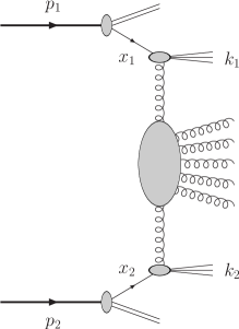
Figure 3.1: Mueller–Navelet jet production process in multi-Regge kinematics.

3.1 Theoretical framework

In this Section the BFKL cross section and the azimuthal corrections for the Mueller–Navelet jet process are presented.

3.1.1 Inclusive dijet production in proton-proton collisions

The reaction under exam is the inclusive production of two jets (a dijet system) in proton-proton collisions

$$p(p_{1})+p(p_{2})\to{\rm jet}(k_{J_{1}})+{\rm jet}(k_{J_{2}})+X\;,$$ (3.1)

where the two jets are characterised by high transverse momenta, $\vec{k}_{J_{1}}^{2}\sim\vec{k}_{J_{2}}^{2}\gg\Lambda_{\rm QCD}^{2}$ and large separation in rapidity; $p_{1}$ and $p_{2}$ are taken as Sudakov vectors (see Eq. (2.10)) satisfying $p_{1}^{2}=p_{2}^{2}=0$ and $2\left(p_{1}p_{2}\right)=s$, working at leading twist and neglecting the proton mass and other power suppressed corrections.

At LHC energies, the theoretical description of this reaction lies at the crossing point of two distinct approaches: collinear factorisation and BFKL resummation. On one side, at leading twist the process can be seen as the hard scattering of two partons, each emitted by one of the colliding hadrons according to the appropriate PDF, see Fig. 3.1. Collinear factorisation takes care to systematically resum the logarithms of the hard scale, through the standard DGLAP evolution of the PDFs and the fixed-order radiative corrections to the parton scattering cross section. The other resummation mechanism at work, justified by the large center-of-mass energy $\sqrt{s}$ available at the LHC, is the BFKL resummation of energy logarithms, which are so large to compensate the small QCD coupling and must therefore be accounted for to all orders of perturbation.

The expression of the cross section (Eq. (2.70)), which takes the form a convolution between two, process-dependent impact factors and a process-independent Green’s function, is valid for a fully inclusive process, i.e. without any particle/object identified/tagged in the final state. By demanding the tagging of two forward jets, each of them produced in the fragmentation region of the respective parent proton, we are relaxing the inclusiveness condition requested in Eq. (2.70). This has an impact on the form of the process-dependent part of the cross section, namely the forward jet impact factors (also known as jet vertices).

Figure 3.2: Schematic view of the forward gluon (left) and the forward quark (right) impact factor. Here $p_{1}$ is the proton momentum, $x_{1}$ is the fraction of proton momentum carried by the parton and $\vec{q}$ is the transverse momentum of the incoming Reggeised gluon.

The starting point is provided by the impact factors for the colliding partons, calculated with NLO accuracy in Refs. [Fadin:1999de, Fadin:1999df] (see Fig. 3.2). To obtain the impact factor for a tagged forward jet (see Fig. 3.3), the first step is to ‘open’ one of the integrations over the intermediate-state phase space to allow one parton to generate the jet . Then, according to QCD collinear factorisation, take the convolution with the parent parton PDFs. The jet can be formed by one parton in LO and by one or two partons when the process is considered in NLO. In the simplest case, the jet momentum is identified with the momentum of the parton in the intermediate state $k$ by the following jet function [Ellis:1989vm]:

$$S_{J}^{(2)}(\vec{k};x)=\delta(x-x_{J})\delta^{(2)}(\vec{k}-\vec{k}_{J})\;,$$ (3.2)

where $x$ is the fraction of proton momentum carried by the quark, $x_{J}$ is the longitudinal fraction of the jet momentum and $\vec{k}_{J}$ is the transverse jet momentum.

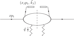
Figure 3.3: Schematic view of the vertex for the forward jet production in the case of incoming gluon (left) or quark (right). Here $p_{1}$ is the proton momentum, $x$ is the fraction of proton momentum carried by the gluon/quark, $x_{J}p_{1}$ is the longitudinal jet momentum, $\vec{k}_{J}$ is the transverse jet momentum and $\vec{q}$ is the transverse momentum of the incoming Reggeised gluon.

We get the expression for the jet impact factor, differential with respect to the variables parameterising the jet phase space, at the LO level as

$$\frac{d\Phi^{(0)}_{J}(\vec{q}\,)}{dx_{J}dk_{J}}=2\pi\alpha_{s}\sqrt{\frac{2C_{F}}{C_{A}}}\int_{0}^{1}dx\left(\frac{C_{A}}{C_{F}}f_{g}(x)+\sum_{a=q,\bar{q}}f_{a}(x)\right)S_{J}^{(2)}(\vec{q};x)\;,$$ (3.3)

given as the sum of the gluon and all possible quark and antiquark PDF contributions $f_{g}(x)$, $f_{a}(x)$. In Eq. (3.3) $C_{F}$ is the colour factor associated with gluon emission from a quark, $C_{F}=(N_{c}^{2}-1)/(2N_{c})$ The last step to do is to project Eq. (3.3) onto the eigenfunctions (Eq. (2.54)) of the LO BFKL kernel (2.53), i.e. transfer to the $(\nu,n)$-representation (see Section 2.3.3). The expression for the LO forward jet vertex will be given in Eq. (3.8) of Section 3.1.3.

In the NLO case, both the one-loop virtual corrections to the amplitude with one parton state and the terms coming from the two-partons final-state amplitude have to be taken into account. In this last case, when the jet originates from a state of two partons, we need another jet selection function $S_{J}^{(3)}$, whose explicit form depends on the chosen jet algorithm. We will use the NLO jet vertex calculated in the small-cone approximation [Furman:1981kf, Aversa:1988vb], i.e. for small jet-cone aperture in the rapidity-azimuthal angle plane, which allow to get a simple analytic result in the $(\nu,n)$-representation (see Eq. (B.1)).

3.1.2 Dijet cross section and azimuthal correlations

In QCD collinear factorisation the cross section of the process (3.1) reads

$$\frac{d\sigma}{dx_{J_{1}}dx_{J_{2}}d^{2}k_{J_{1}}d^{2}k_{J_{2}}}=\sum_{r,s=q,{\bar{q}},g}\int_{0}^{1}dx_{1}\int_{0}^{1}dx_{2}\ f_{r}\left(x_{1},\mu_{F}\right)\ f_{s}\left(x_{2},\mu_{F}\right)$$ (3.4)

$$=\frac{d{\hat{\sigma}}_{r,s}\left(x_{1}x_{2}s,\mu_{F}\right)}{dx_{J_{1}}dx_{J_{2}}d^{2}k_{J_{1}}d^{2}k_{J_{2}}}\;,$$

where the $r,s$ indices specify the parton types (quarks $q=u,d,s,c,b$; antiquarks $\bar{q}=\bar{u},\bar{d},\bar{s},\bar{c},\bar{b}$; or gluon $g$), $f_{i}\left(x,\mu_{F}\right)$ denotes the initial proton PDFs; $x_{1,2}$ are the longitudinal fractions of the partons involved in the hard subprocess, while $x_{J_{1,2}}$ are the jet longitudinal fractions; $\mu_{F}$ is the factorisation scale; $d\hat{\sigma}_{r,s}\left(x_{1}x_{2}s,\mu_{F}\right)$ is the partonic cross section for the production of jets and $x_{1}x_{2}s\equiv\hat{s}$ is the squared center-of-mass energy of the parton-parton collision subprocess (see Fig. 3.1).

The cross section of the process can be presented as (see Section 2.3.3 for the details of the derivation)

$$\frac{d\sigma}{dy_{J_{1}}dy_{J_{2}}\,d|\vec{k}_{J_{1}}|\,d|\vec{k}_{J_{2}}|d\phi_{J_{1}}d\phi_{J_{2}}}=\frac{1}{(2\pi)^{2}}\left[{\cal C}_{0}+\sum_{n=1}^{\infty}2\cos(n\phi)\,{\cal C}_{n}\right]\,,$$ (3.5)

where $\phi=\phi_{J_{1}}-\phi_{J_{2}}-\pi$, while ${\cal C}_{0}$ gives the total cross section and the other coefficients ${\cal C}_{n}$ determine the distribution of the azimuthal angle of the two jets.

Since the main object of the present analysis is the impact of jet produced in the central region on azimuthal coefficients, we will concentrate just on one representation for ${\cal C}_{n}$, out of the many possible NLA-equivalent options (see Section. 2.3.3.1 for a discussion). In particular, we will use the exponentiated representation together with the BLM optimisation method, whose details are given in Section 2.4 on scale $\mu_{R}$ and the factorisation scale $\mu_{F}$. In our calculation we will use the exact implementation of BLM method, given in Eq. (2.84), together with the two approximate, semianalytic $(a)$ and $(b)$ cases (Eqs. (2.85) and (2.87), respectively), in order to keep contact with with previous applications of BLM method where approximate approaches were used.

3.1.3 BLM scale setting

In this Section the expressions for the azimuthal coefficients ${\cal C}_{n}$, using the BLM prescription (see Section 2.4) are given. For the approximated $(a)$ (Eq. (2.86)) and $(b)$ (Eq. (2.88)) cases, we present also the expressions in the fixed-order DGLAP approach at the NLO, which will be used in the phenomenology Section 3.3. The ${\cal C}_{n}^{\rm DGLAP}$ coefficients are nothing but the truncation of the respective BFKL expressions ${\cal C}_{n}$ up to inclusions of NLO terms.

Introducing, for the sake of brevity, the definitions

$$Y=y_{J_{1}}-y_{J_{2}}=\ln\frac{x_{J_{1}}x_{J_{2}}s}{|\vec{k}_{J_{1}}||\vec{k}_{J_{2}}|}\;,\;\;\;\;\;Y_{0}=\ln\frac{s_{0}}{|\vec{k}_{J_{1}}||\vec{k}_{J_{2}}|}\;,$$ (3.6)

we will present in what follows the three different expressions for the coefficients ${\cal C}_{n}$.

$\bullet$ case “exact”

We remember that the BLM optimal scale $\mu_{R}^{\rm BLM}$ is defined as the value of $\mu_{R}$ that makes all contributions to the considered observables which are proportional to the QCD $\beta-$ function, $\beta_{0}$, vanish, such that Eq. (2.83) is satisfied. After that we have the following expression for our observables:

$${\cal C}_{n}=\frac{x_{J_{1}}x_{J_{2}}}{|\vec{k}_{J_{1}}||\vec{k}_{J_{2}}|}\int_{-\infty}^{+\infty}d\nu\ e^{(Y-Y_{0})\bar{\alpha}_{s}^{\rm MOM}(\mu_{R}^{\rm BLM})\left[\chi+\bar{\alpha}_{s}^{\rm MOM}(\mu_{R}^{\rm BLM})\left(\bar{\chi}+\frac{T^{\rm conf}}{N_{c}}\chi\right)\right]}$$ (3.7)

$$\times\,(\alpha_{s}^{\rm MOM}(\mu_{R}^{\rm BLM}))^{2}c_{1}(n,\nu,|\vec{k}_{J_{1}}|,x_{J_{1}})c_{2}(n,\nu,|\vec{k}_{J_{2}}|,x_{J_{2}})$$

$$\times\,\left[1+\alpha_{s}^{\rm MOM}(\mu_{R}^{\rm BLM})\left\{\frac{\bar{c}_{1}^{\left(1\right)}(n,\nu,|\vec{k}_{J_{1}}|,x_{J_{1}})}{c_{1}(n,\nu,|\vec{k}_{J_{1}}|,x_{J_{1}})}+\frac{\bar{c}_{2}^{\left(1\right)}(n,\nu,|\vec{k}_{J_{2}}|,x_{J_{2}})}{c_{2}(n,\nu,|\vec{k}_{J_{2}}|,x_{J_{2}})}+\frac{2T^{\rm conf}}{N_{c}}\right\}\right]\;.$$

In the above equation, $\alpha_{s}^{\rm MOM}$ is the QCD coupling in the physical momentum subtraction (MOM) scheme, related to $\alpha_{s}^{\overline{\rm MS}}$ by the finite renormalisation given in Eq. (2.80), while ${\bar{\alpha}_{s}^{\rm MOM}}=N_{c}/\pi\,\alpha_{s}^{\rm MOM}$ as in Eq. (2.51), with $N_{c}$ the number of colours. Then,

$$c_{1}(n,\nu,|\vec{k}|,x)=2\sqrt{\frac{C_{F}}{C_{A}}}(\vec{k}^{\,2})^{i\nu-1/2}\,\left(\frac{C_{A}}{C_{F}}f_{g}(x,\mu_{F})+\sum_{a=q,\bar{q}}f_{a}(x,\mu_{F})\right)$$ (3.8)

and

$$c_{2}(n,\nu,|\vec{k}|,x)=\biggl{[}c_{1}(n,\nu,|\vec{k}|,x)\biggr{]}^{*}\;,$$ (3.9)

are the LO jet vertices in the $\nu$-representation (see Eq. (3.3) for the corresponding expression in the momentum space) and $\chi=\chi(n,\nu)$ is the eigenvalue of the LO BFKL kernel (Eq. (2.53)). Note that, since $c_{1,2}$ do not depend on $\nu$, the $f(\nu)$ function, whose general expression is given in Eq. (2.77), is zero for this process. The remaining objects are related to the NLO corrections of the BFKL kernel, ($\bar{\chi}(n,\nu)$, given in Eq. (2.60)) and of the jet vertices in the small-cone approximation ($c_{1,2}^{(1)}(n,\nu,|\vec{k}_{J_{1,2}}|,x_{J_{1,2}})$, given in Eq. (B.1) of Appendix B. The functions $\bar{c}_{1,2}^{(1)}(n,\nu,|\vec{k}_{J_{2}}|,x_{J_{2}})$ are the same as $c_{1,2}^{(1)}(n,\nu,|\vec{k}_{J_{1,2}}|,x_{J_{1,2}})$ with all terms proportional to $\beta_{0}$ removed.

$\bullet$ case $(a)$

$$(\mu_{R,a}^{\rm BLM})^{2}=k_{J_{1}}k_{J_{2}}\exp\left[2\left(1+\frac{2}{3}I\right)-\frac{5}{3}\right]\;,$$

with

$${\cal C}_{n}^{\rm(a)}=\frac{x_{J_{1}}x_{J_{2}}}{|\vec{k}_{J_{1}}||\vec{k}_{J_{2}}|}\int_{-\infty}^{+\infty}d\nu\ e^{(Y-Y_{0})\left[\bar{\alpha}_{s}^{\rm MOM}(\mu_{R,a}^{\rm BLM})\chi+(\bar{\alpha}_{s}^{\rm MOM}(\mu_{R,a}^{\rm BLM}))^{2}\left(\bar{\chi}+\frac{T^{\rm conf}}{N_{c}}\chi-\frac{\beta_{0}}{8N_{c}}\chi^{2}\right)\right]}$$ (3.10)

$$\times\,(\alpha_{s}^{\rm MOM}(\mu_{R,a}^{\rm BLM}))^{2}c_{1}(n,\nu,|\vec{k}_{J_{1}}|,x_{J_{1}})c_{2}(n,\nu,|\vec{k}_{J_{2}}|,x_{J_{2}})$$

$$\times\,\left[1+\alpha_{s}^{\rm MOM}(\mu_{R,a}^{\rm BLM})\left\{\frac{\bar{c}_{1}^{\left(1\right)}(n,\nu,|\vec{k}_{J_{1}}|,x_{J_{1}})}{c_{1}(n,\nu,|\vec{k}_{J_{1}}|,x_{J_{1}})}+\frac{\bar{c}_{2}^{\left(1\right)}(n,\nu,|\vec{k}_{J_{2}}|,x_{J_{2}})}{c_{2}(n,\nu,|\vec{k}_{J_{2}}|,x_{J_{2}})}+\frac{2T^{\rm conf}}{N_{c}}\right\}\right]\;;$$

$${\cal C}_{n}^{\rm DGLAP\,(a)}=\frac{x_{J_{1}}x_{J_{2}}}{|\vec{k}_{J_{1}}||\vec{k}_{J_{2}}|}\int_{-\infty}^{+\infty}d\nu\ \alpha_{s}^{2}c_{1}(n,\nu,|\vec{k}_{J_{1}}|,x_{J_{1}})c_{2}(n,\nu,|\vec{k}_{J_{2}}|,x_{J_{2}})$$ (3.11)

$$\times\,\left[1+\frac{2}{\pi}\alpha_{s}T^{\rm conf}+\bar{\alpha}_{s}\left(Y-Y_{0}\right)\chi\right.$$

$$\left.+\,\alpha_{s}\left(\frac{\bar{c}_{1}^{\left(1\right)}(n,\nu,|\vec{k}_{J_{1}}|,x_{J_{1}})}{c_{1}(n,\nu,|\vec{k}_{J_{1}}|,x_{J_{1}})}+\frac{\bar{c}_{2}^{\left(1\right)}(n,\nu,|\vec{k}_{J_{2}}|,x_{J_{2}})}{c_{2}(n,\nu,|\vec{k}_{J_{2}}|,x_{J_{2}})}\right)\right]\;,$$

$\bullet$ case $(b)$

$$(\mu_{R,b}^{\rm BLM})^{2}=k_{J_{1}}k_{J_{2}}\exp\left[2\left(1+\frac{2}{3}I\right)-\frac{5}{3}+\frac{1}{2}\,\chi(n,\nu)\right]\;,$$

with

$${\cal C}_{n}^{(b)}=\frac{x_{J_{1}}x_{J_{2}}}{|\vec{k}_{J_{1}}||\vec{k}_{J_{2}}|}\int_{-\infty}^{+\infty}d\nu\ e^{(Y-Y_{0})\left[\bar{\alpha}_{s}^{\rm MOM}(\mu_{R,b}^{\rm BLM})\chi+(\bar{\alpha}_{s}^{\rm MOM}(\mu_{R,b}^{\rm BLM}))^{2}\left(\bar{\chi}+\frac{T^{\rm conf}}{N_{c}}\chi\right)\right]}$$ (3.12)

$$\times\,(\alpha_{s}^{\rm MOM}(\mu_{R,b}^{\rm BLM}))^{2}c_{1}(n,\nu,|\vec{k}_{J_{1}}|,x_{J_{1}})c_{2}(n,\nu,|\vec{k}_{J_{2}}|,x_{J_{2}})$$

$$\times\,\left[1+\alpha_{s}^{\rm MOM}(\mu_{R,b}^{\rm BLM})\left\{\frac{\bar{c}_{1}^{\left(1\right)}(n,\nu,|\vec{k}_{J_{1}}|,x_{J_{1}})}{c_{1}(n,\nu,|\vec{k}_{J_{1}}|,x_{J_{1}})}+\frac{\bar{c}_{2}^{\left(1\right)}(n,\nu,|\vec{k}_{J_{2}}|,x_{J_{2}})}{c_{2}(n,\nu,|\vec{k}_{J_{2}}|,x_{J_{2}})}+\frac{2T^{\rm conf}}{N_{c}}+\frac{\beta_{0}}{4N_{c}}\chi\right\}\right]\;,$$

$${\cal C}_{n}^{\rm DGLAP\,(b)}=\frac{x_{J_{1}}x_{J_{2}}}{|\vec{k}_{J_{1}}||\vec{k}_{J_{2}}|}\int_{-\infty}^{+\infty}d\nu\ \alpha_{s}^{2}c_{1}(n,\nu,|\vec{k}_{J_{1}}|,x_{J_{1}})c_{2}(n,\nu,|\vec{k}_{J_{2}}|,x_{J_{2}})$$ (3.13)

$$\times\,\left[1+\alpha_{s}\left(\mu_{R}\right)\left(\frac{\beta_{0}}{4\pi}\chi+2\frac{T^{\rm conf}}{\pi}\right)+\bar{\alpha}_{s}\left(Y-Y_{0}\right)\chi\right.$$

$$\left.+\,\alpha_{s}\left(\frac{\bar{c}_{1}^{\left(1\right)}(n,\nu,|\vec{k}_{J_{1}}|,x_{J_{1}})}{c_{1}(n,\nu,|\vec{k}_{J_{1}}|,x_{J_{1}})}+\frac{\bar{c}_{2}^{\left(1\right)}(n,\nu,|\vec{k}_{J_{2}}|,x_{J_{2}})}{c_{2}(n,\nu,|\vec{k}_{J_{2}}|,x_{J_{2}})}\right)\right]\;.$$

Note that, in the above equations the scale $s_{0}$ entering $Y_{0}$ is the artificial energy scale introduced in the BFKL approach to perform the Mellin transform from the $s$-space to the complex angular momentum plane and cancels in the full expression, up to terms beyond the NLA. In our analysis it will always be fixed at the “natural” value $Y_{0}=0$, given by the kinematical of Mueller–Navelet process.

Although the final expressions in Eqs. (3.7), (3.10), (3.11), (3.12), and (3.13) are given in terms of $\alpha^{\rm MOM}$ in the MOM scheme, it is possible to use analogous expressions in the $\overline{\rm MS}$ scheme. The way to do that is to start from the general expressions, then perform the change of scheme $\overline{\rm MS}$ $\to$ MOM as an intermediate step, and finally, after setting the BLM scales, go back again to the $\overline{\rm MS}$ scheme. From a practical point of view, one obtains the expressions in the $\overline{\rm MS}$ scheme, starting from MOM, by making the change

$$T^{\rm conf}\,\to\,-T^{\beta}\;,$$ (3.14)

with $T^{\beta}$ given in Eq. (2.81), in the expressions cited above. In Sections 3.2 and 3.3 we will give predictions for our observables in the $\overline{\rm MS}$ scheme.

3.1.4 Integration over the final-state phase space

In order to match the kinematical cuts used by the CMS collaboration (see for instance Ref. [Khachatryan:2016udy]), we will consider the integrated coefficients given by

$$\int_{y_{J_{2}}^{\rm min}}^{y_{J_{2}}^{\rm max}}dy_{J_{2}}\int_{k_{J_{1}}^{\rm min}}^{\infty}dk_{J_{1}}\int_{k_{J_{2}}^{\rm min}}^{\infty}dk_{J_{2}}\,\delta\left(y_{J_{1}}-y_{J_{2}}-Y\right)$$ (3.15)

$$\times\,{\cal C}_{n}\left(y_{J_{1}},y_{J_{2}},k_{J_{1}},k_{J_{2}}\right)$$

and their ratios $R_{nm}\equiv C_{n}/C_{m}$. Among them, the ratios of the form $R_{n0}$ have a simple physical interpretation, being the azimuthal correlations $\langle\cos(n\phi)\rangle$. We will take jet rapidities in the range delimited by $y_{J_{1}}^{\rm min}=y_{J_{2}}^{\rm min}=-4.7$ and $y_{J_{1}}^{\rm max}=y_{J_{2}}^{\rm max}=4.7$ and study the dependence of the $R_{nm}$ ratios as function of the jet rapidity separation $Y\equiv y_{J_{1}}-y_{J_{2}}$. Concerning the jet transverse momenta $k_{J_{1,2}}$, differently from most previous analyses, we make several different choices, which include asymmetric cuts (see the next three Sections for further details). The jet-cone size $R$ entering the NLO-jet vertices is fixed at the value $R=0.5$ and, as anticipated, $Y_{0}=0$. Finally, we will consider two characteristic values for the center-of-mass energy, i.e. $\sqrt{s}=7$ TeV, for which experimental anaylises with symmetric configuration for the outgoing jet momenta already exist (see Section 3.2), and $\sqrt{s}=13$ TeV.

3.2 Theory versus experiment

In this Section we present the analysis of Ref. [Caporale:2014gpa], in which predictions for the $R_{10}$, $R_{20}$, $R_{30}$, $R_{21}$ and $R_{32}$ are given and compared with recent CMS data at $7$ TeV [Khachatryan:2016udy]. BLM scale optimisation, in both variants $(a)$ (Eq. (3.10)) and $(b)$ (Eq. (3.12)) is used, while final calculations are done in the $\overline{\rm MS}$. We remember that the expressions above cited are given in the MOM scheme and it is possible to obtain the analogous ones in the $\overline{\rm MS}$ through the substitution $T^{\rm conf}\to-T^{\beta}$, with $T^{\rm conf}$ and $T^{\beta}$ given in Eq. (2.81).

Results are reported in Table 3.1 and in Fig. 3.4. We clearly see that the pure LLA calculations (i.e. considering just the LO kernel contribution and neglecting the NLO corrections to the impact factors) overestimate the decorrelation by far in all $R_{nm}$ ratios. Introducing NLA BFKL corrections and using the BLM method we can see that, except for the ratio $C_{1}/C_{0}$, the agreement with experimental data becomes very good, for both variants $(a)$ and $(b)$, at the larger values of $Y$.

Meanwhile, it would be also useful to address, on the experimental side, some possible issues which could be sources of mismatch with the way in which Mueller–Navelet jets are defined in theory and that are not easy to be revealed in the comparison with theoretical predictions, for being the latter affected in their turn by systematic effects of the same amount. We list below two of them.

• The use of symmetric cuts in the values of $k_{J_{i}}^{\rm min}$ maximises the contribution of the Born term in $C_{0}$, which is present for back-to-back jets (see Fig. 3.5) only and is expected to be large, therefore making less visible the effect of the BFKL resummation in all observables involving $C_{0}$. The use of asymmetric cuts can reduce the contribution of the Born term and enhance effects with additional undetected hard gluon radiation, which makes the visibility of BFKL effect more clear in comparison to the descriptions based on fixed-order DGLAP approach.

• In data analysis defining the $Y$ value for a given final state with two jets, the rapidity of one of the two jets could be so small, say $|y_{J_{i}}|\lesssim 2$, that this jet is actually produced in the central region, rather than in one of the two forward regions. The longitudinal momentum fractions of the parent partons that generate a central jet are very small, and one can naturally expect sizable corrections to the vertex of this jet, due to the fact that the collinear factorisation approach used in the derivation of the result for jet vertex is not designed for the region of small $x$.

These issues are addressed in Sections 3.3 and 3.4, respectively.

Table 3.1: $R_{10}$, $R_{20}$, $R_{30}$, $R_{21}$, and $R_{32}$ with the BLM method, in both variants $(a)$ (Eq. (3.10)) and $(b)$ (Eq. (3.12)).

	$C_{1}/C_{0}$		$C_{2}/C_{0}$		$C_{3}/C_{0}$		$C_{2}/C_{1}$		$C_{3}/C_{2}$
$Y$	$(a)$	$(b)$	$(a)$	$(b)$	$(a)$	$(b)$	$(a)$	$(b)$	$(a)$	$(b)$
3	0.960	0.962	0.819	0.821	0.687	0.696	0.853	0.853	0.839	0.848
4	0.890	0.892	0.684	0.696	0.548	0.555	0.768	0.780	0.798	0.797
5	0.837	0.818	0.582	0.587	0.427	0.434	0.696	0.713	0.733	0.744
6	0.744	0.744	0.447	0.483	0.320	0.335	0.627	0.649	0.686	0.694
7	0.685	0.680	0.387	0.403	0.246	0.261	0.566	0.593	0.636	0.647
8	0.660	0.641	0.339	0.348	0.202	0.213	0.513	0.544	0.596	0.611
9	0.760	0.663	0.367	0.344	0.207	0.201	0.483	0.519	0.563	0.583

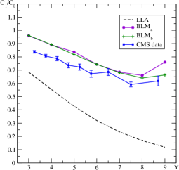
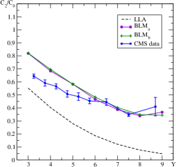
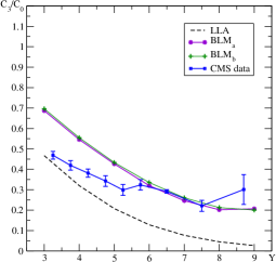
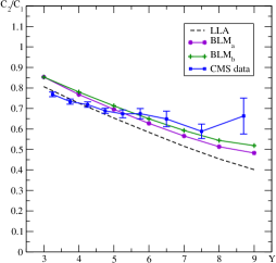
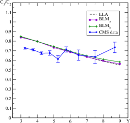
Figure 3.4: $Y$-dependence of $R_{10}$, $R_{20}$, $R_{30}$, $R_{21}$, and $R_{32}$ at $\sqrt{s}=7$ TeV [Khachatryan:2016udy] in the symmetric configuration $k_{J_{1,2}}^{\rm min}=35$ GeV. Results were obtained with the two variants $(a)$ (Eq. (3.10)) and $(b)$ (Eq. (3.12)) of the BLM method. The dashed line gives the LLA BFKL result.

3.3 BFKL versus high-energy DGLAP

3.3.1 Motivation

As we saw at the end of Section 3.2, the effect of Born contribution to the cross section $C_{0}$, present only for back-to-back jets (see Fig. 3.5), is maximised when symmetric cuts in the values of the forward jet transverse momenta are used; on the contrary, in the case of asymmetric cuts, the Born term is suppressed and the effects of the additional undetected hard gluon radiation is enhanced, thus making more visible the BFKL resummation, in comparison to descriptions based on the fixed-order DGLAP approach, in all observables involving $C_{0}$.

For this purpose, we compare predictions for several azimuthal correlations and their ratios obtained, on one side, by a fixed-order DGLAP calculation at the NLO and, on the other side, by BFKL resummation in the NLA.

We remember that our implementation of the NLO DGLAP calculation is an approximate one. We just use here NLA BFKL expressions, given in Eqs. (3.11) and (3.13), for the observables that are truncated to the ${\cal O}\left(\alpha_{s}^{3}\right)$ order. In this way we take into account the leading power asymptotic of the exact NLO DGLAP prediction and neglect terms that are suppressed by the inverse powers of the energy of the parton-parton collisions. Such approach is legitimate in the region of large $Y$ which we consider here. The exact implementation of NLO DGLAP for Mueller–Navelet jets is important, because it allows to understand better the region of applicability of our approach, but it requires more involved Monte Carlo calculations. We use the BLM scheme in both semianalytic $(a)$ (Eq. (2.86)) and $(b)$ (Eq. (2.88)) cases in order to compare BFKL (Eqs. (3.10) and (3.12) with DGLAP (Eqs. (3.11) and (3.11) predictions. As done in Section 3.2, we perform all calculations in the $\overline{\rm MS}$ scheme. We remember that all the four expressions above cited are given in the MOM scheme and it is possible to obtain the analogous ones in the $\overline{\rm MS}$ through the substitution $T^{\rm conf}\to-T^{\beta}$, with $T^{\rm conf}$ and $T^{\beta}$ given in (2.81).

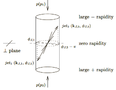
Figure 3.5: Mueller–Navelet jets at LLA: a back-to-back dijet reaction. Picture from Ref. [Colferai:2010wu].

Another important benefit from the use of asymmetric cuts, pointed out in [Ducloue:2014koa], is that the effect of violation of the energy-momentum conservation in the NLA is strongly suppressed with respect to what happens in the LLA.

3.3.2 Results and discussion

We study the $Y$-dependence of ratios $R_{nm}$ of the integrated coefficients given in Eq. (3.15), fixing the center-of-mass energy at $\sqrt{s}=7$ TeV and making two asymmetric choices for the jet transverse momenta:

1. $k_{J_{1}}^{\rm min}=35\,\text{GeV},\quad\quad\quad k_{J_{2}}^{\rm min}=45\,\text{GeV};$

2. $k_{J_{1}}^{\rm min}=35\,\text{GeV},\quad\quad\quad k_{J_{2}}^{\rm min}=50\,\text{GeV}.$

We summarise our results in Tables 3.2 and 3.3 and in Figs. 3.6 and 3.7. We can clearly see that, at $Y=9$, BFKL and DGLAP, in both variants $(a)$ (Eq. (3.10)) and $(b)$ (Eq. (3.12)) of the BLM setting, give quite different predictions for the all considered ratios except $C_{1}/C_{0}$; at $Y=6$ this happens in fewer cases, while at $Y=3$ BFKL and DGLAP cannot be distinguished with given uncertainties. In particular, taking one of the cuts at 35 GeV (as done by the CMS collaboration [Khachatryan:2016udy]) and the other at 45 GeV or 50 GeV, we can clearly see that predictions from BFKL and DGLAP become separate for most azimuthal correlations and ratios between them, this effect being more and more visible as the rapidity gap between the jets, $Y$, increases. In other words, in this kinematics the additional undetected parton radiation between the jets which is present in the resummed BFKL series, in comparison to just one undetected parton allowed by the NLO DGLAP approach, makes its difference and leads to more azimuthal angle decorrelation between the jets, in full agreement with the original proposal of Mueller and Navelet.

This result was not unexpected: the use of symmetric cuts for jet transverse momenta maximises the contribution of the Born term, which is present for back-to-back jets only and is expected to be large, therefore making less visible the effect of the BFKL resummation. This phenomenon could be at the origin of the instabilities observed in the NLO fixed-order calculations of Refs. [Andersen:2001kta, Fontannaz:2001nq].

One may argue that using disjoint intervals for the two jet transverse momenta would be an even cleaner setup. However, since the majority of dijet events are characterised by the lowest possible values for the jet transverse momenta in the selected range, our setup with two different lower cuts but overlapping intervals is not effectively different from the setup with disjoint transverse momenta ranges. Furthermore, independently of the cutoff procedure, there is a non-escapable limitation, namely that the actual energies of partonic subprocesses at the LHC are not much larger than the final-object transverse momenta and, therefore, not too many additional hard parton emissions can occur. This implies that, even after asymmetric or disjoint configurations in the transverse momentum space, the BFKL and the full NLO DGLAP approaches are not expected to be largely different.

Table 3.2: Ratios $C_{n}/C_{m}$ at 7 TeV and for $k_{J_{1}}^{\rm min}=35$ GeV and $k_{J_{2}}^{\rm min}=45$ GeV.

	$Y$	BFKL${}_{(a)}$	DGLAP${}_{(a)}$	BFKL${}_{(b)}$	DGLAP${}_{(b)}$
	3.0	0.963(21)	1.003(44)	0.964(17)	1.021(78)
$C_{1}/C_{0}$	6.0	0.7426(43)	0.884(61)	0.7433(30)	0.914(91)
	9.0	0.897(15)	0.868(16)	0.714(10)	0.955(50)
	3.0	0.80(2)	0.948(43)	0.812(15)	0.949(75)
$C_{2}/C_{0}$	6.0	0.4588(32)	0.726(56)	0.4777(26)	0.702(81)
	9.0	0.4197(79)	0.710(15)	0.3627(50)	0.850(48)
	3.0	0.672(18)	0.876(41)	0.684(13)	0.838(70)
$C_{3}/C_{0}$	6.0	0.3095(26)	0.566(45)	0.3282(21)	0.435(68)
	9.0	0.2275(72)	0.558(13)	0.2057(29)	0.717(44)
	3.0	0.831(18)	0.945(43)	0.842(16)	0.929(72)
$C_{2}/C_{1}$	6.0	0.6178(43)	0.821(66)	0.6427(34)	0.768(91)
	9.0	0.4677(63)	0.817(18)	0.5079(56)	0.890(51)
	3.0	0.839(22)	0.924(45)	0.843(17)	0.883(76)
$C_{3}/C_{2}$	6.0	0.6745(64)	0.780(71)	0.6869(52)	0.62(11)
	9.0	0.542(15)	0.787(21)	0.5670(59)	0.844(56)

Table 3.3: Ratios $C_{n}/C_{m}$ at 7 TeV and for $k_{J_{1}}^{\rm min}=35$ GeV and $k_{J_{2}}^{\rm min}=50$ GeV.

	$Y$	BFKL${}_{(a)}$	DGLAP${}_{(a)}$	BFKL${}_{(b)}$	DGLAP${}_{(b)}$
	3.0	0.961(23)	1.006(46)	0.964(15)	1.034(89)
$C_{1}/C_{0}$	6.0	0.7360(49)	0.869(58)	0.7357(25)	0.89(12)
	9.0	1.0109(61)	0.857(16)	0.7406(46)	0.958(56)
	3.0	0.788(21)	0.946(44)	0.801(14)	0.950(85)
$C_{2}/C_{0}$	6.0	0.4436(37)	0.698(53)	0.4626(19)	0.611(98)
	9.0	0.4568(50)	0.695(15)	0.3629(23)	0.862(54)
	3.0	0.653(19)	0.868(43)	0.669(12)	0.814(79)
$C_{3}/C_{0}$	6.0	0.2925(31)	0.530(42)	0.3115(15)	0.320(57)
	9.0	0.2351(35)	0.551(17)	0.1969(17)	0.748(50)
	3.0	0.820(21)	0.940(44)	0.832(15)	0.918(81)
$C_{2}/C_{1}$	6.0	0.6027(51)	0.803(64)	0.6288(26)	0.69(12)
	9.0	0.4518(35)	0.811(18)	0.4900(24)	0.899(57)
	3.0	0.829(26)	0.917(46)	0.835(17)	0.857(85)
$C_{3}/C_{2}$	6.0	0.6595(82)	0.759(70)	0.6733(36)	0.52(11)
	9.0	0.5146(85)	0.793(23)	0.5426(38)	0.869(62)

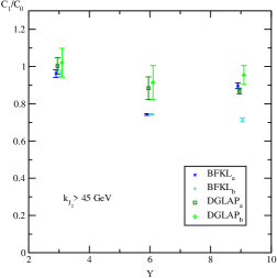
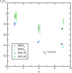
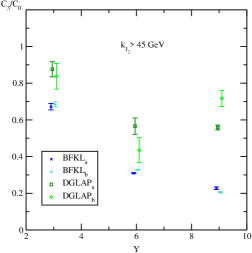
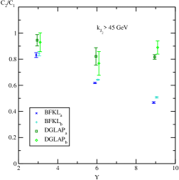
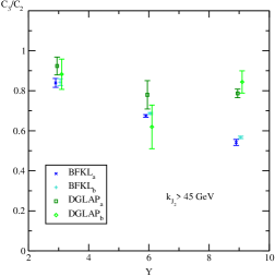
Figure 3.6: $Y$-dependence of several ratios $C_{m}/C_{n}$ for $k_{J_{1}}^{\rm min}=35$ GeV and $k_{J_{2}}^{\rm min}=45$ GeV, for BFKL and high-energy DGLAP in the two variants $(a)$ (Eq. (3.10)) and $(b)$ (Eq. (3.12)) of the BLM method and for $\sqrt{s}=7$ TeV (data points have been slightly shifted along the horizontal axis for the sake of readability).

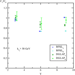
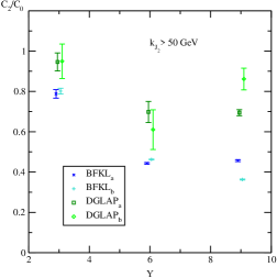
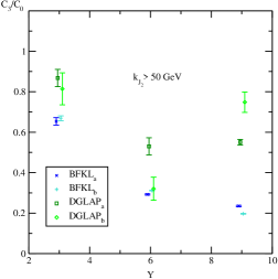
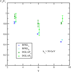
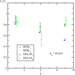
Figure 3.7: $Y$-dependence of several ratios $C_{m}/C_{n}$ for $k_{J_{1}}^{\rm min}=35$ GeV and $k_{J_{2}}^{\rm min}=50$ GeV, for BFKL and high-energy DGLAP in the two variants $(a)$ (Eq. (3.10)) and $(b)$ (Eq. (3.12)) of the BLM method and for $\sqrt{s}=7$ TeV (data points have been slightly shifted along the horizontal axis for the sake of readability).

3.4 Central rapidity range exclusion

3.4.1 Motivation

In the last Section we studied the effect of using asymmetric cuts for the jet transverse momenta, comparing full NLA BFKL predictions with fixed-order DGLAP calculations in the high-energy limit. Here we want do deal with another issue, which deserves some care and has not been taken into consideration both in theoretical and experimental analyses so far. As anticipated in the discussion at the end of Section 3.2, in defining the jet rapidity separation $Y$ for a given final state with two jets, the rapidity of one of the two jets could be so small, say $|y_{J_{i}}|\lesssim 2$, that this jet is actually produced in the central region, rather than in one of the two forward regions. Since the longitudinal momentum fractions of the parent partons $x$ that generate such central jet are very small, one can naturally expect sizable corrections to the vertex of this jet, due to the fact that the collinear factorisation approach used in the derivation of the result for jet vertex could not be accurate enough in our kinematical region, where $x$ values can be as small as, $x\sim 10^{-3}$.

The use of collinear factorisation methods in the case of central jet production in our kinematical range deserves some discussion. On one hand, at $x\sim 10^{-3}$ and at scales of the order of the jet transverse momenta which we consider here, $\sim 20\div 40$ GeV, PDFs are well constrained, mainly from DIS HERA data. On the other hand, in this kinematical region PDF parameterisations extracted in next-to-NLO (NNLO) and in NLO approximations start to differ one from the other, which indicates that NNLO effects become essential in the DIS cross sections. The situation with central jet production in proton-proton collisions may be different. Recently, in Ref. [Currie:2013dwa] results for NNLO corrections to the dijet production originated from the gluonic subprocesses were presented. In the region $|y_{J_{1,2}}|<0.3$ and for jet transverse momenta $\sim 100$ GeV, the account of NNLO effects leads to an increase of the cross section by $\sim 25\$. For our kinematics, featuring smaller jet transverse momenta and “less inclusive” coverage of jet rapidities, one could expect even larger NNLO corrections.

Conceptually, instead of the collinear approach, for jets produced in the central rapidity region (at very small $x$) a promising approach would be to use a high-energy factorisation scheme (often also referred as $k_{T}$-factorisation) [Catani:1990eg, Collins:1991ty, Gribov:1984tu, Levin:1991ry] together with the NLO central jet vertex calculated in Ref. [Bartels:2006hg] .

We suggest to compare BFKL theory predictions with data in a region where theoretical uncertainties related to other kind of physics are most possibly reduced. Therefore we propose to return to the original Mueller–Navelet idea, to study the inclusive production of two forward jets separated by a large rapidity gap, and to remove from the analysis those regions where jets are produced at central rapidities.

As a contribution to the assessment of this effect, in this Section we will study the $Y$-dependence of several azimuthal correlations and ratios among them, imposing an additional constraint, that the rapidity of a Mueller–Navelet jet cannot be smaller than a given value. Then we will compare this option with the case when the constraint is absent.

3.4.2 Phase-space constraints

In order to exclude events where, for a given $Y$, one of the two jets is produced in the central region, we need to slightly modify the definition of the integrated coefficients given in Eq. (3.15) in the following way:

$$C_{n}=\int_{y_{J_{1}}^{\rm min}}^{y_{J_{1}}^{\rm max}}dy_{1}\int_{y_{J_{2}}^{\rm min}}^{y_{J_{2}}^{\rm max}}dy_{2}\int_{k_{J_{1}}^{\rm min}}^{\infty}dk_{J_{1}}\int_{k_{J_{2}}^{\rm min}}^{\infty}dk_{J_{2}}\delta\left(y_{J_{1}}-y_{J_{2}}-Y\right)$$ (3.16)

$$\times\,\theta\left(|y_{J_{1}}|-y^{\rm C}_{\rm max}\right)\theta\left(|y_{J_{2}}|-y^{\rm C}_{\rm max}\right){\cal C}_{n}\left(y_{J_{1}},y_{J_{2}},k_{J_{1}},k_{J_{2}}\right)\;.$$

In Eq. (3.16), the two step-functions force the exclusion of jets whose rapidity is smaller than a cutoff value, given by $y^{\rm C}_{\rm max}$, which delimits the central rapidity region (see Fig. 3.8 for a schematic view).

As for the values of $y^{\rm C}_{\rm max}$, we will consider three cases: $y^{\rm C}_{\rm max}=0$, which means no exclusion from jets in the central region, as in all the numerical analyses so far; $y^{\rm C}_{\rm max}=1.5$, corresponding to a central region with size equal to about one third of the maximum possible rapidity span $Y=9.4$ and $y^{\rm C}_{\rm max}=2.5$, a control value, to check the stability of our results.

Concerning the jet transverse momenta, differently from most previous analyses, we make the following five choices, which include asymmetric cuts:

1. $k_{J_{1}}^{\rm\,min}=20\,\text{GeV},\quad\quad\quad k_{J_{2}}^{\rm\,min}=20\,\text{GeV};$

2. $k_{J_{1}}^{\rm\,min}=20\,\text{GeV},\quad\quad\quad k_{J_{2}}^{\rm\,min}=30\,\text{GeV};$

3. $k_{J_{1}}^{\rm\,min}=20\,\text{GeV},\quad\quad\quad k_{J_{2}}^{\rm\,min}=35\,\text{GeV};$

4. $k_{J_{1}}^{\rm\,min}=20\,\text{GeV},\quad\quad\quad k_{J_{2}}^{\rm\,min}=40\,\text{GeV};$

5. $k_{J_{1}}^{\rm\,min}=35\,\text{GeV},\quad\quad\quad k_{J_{2}}^{\rm\,min}=35\,\text{GeV};$

We will give the first phenomenological predictions for the ratios $R_{nm}\equiv C_{n}/C_{m}$ at center-of-mass energy $\sqrt{s}=13$ TeV, using the BLM scheme in its exact implementation (Eq. (3.7)). We will perform also some calculations with these approximate schemes $(a)$ (Eq. (3.10)) and $(b)$ (Eq. (3.12)), in order to get an idea about the inaccuracy of our predictions coming from such approximate implementations of the BLM scale setting. Differently from Sections 3.2 and 3.3, all calculations are done in the MOM renormalisation scheme.

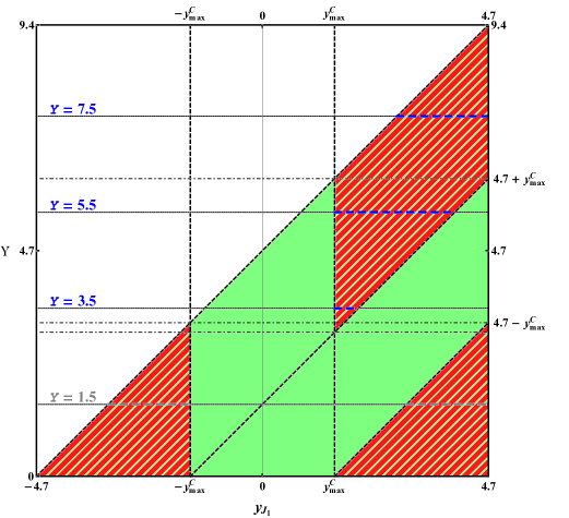
Figure 3.8: Central rapidity range exclusion in the $(y_{J_{1}},Y)$ phase-subspace for Mueller–Navelet jets. The green triangle represents the area bounded by the kinematical cuts on $y_{J_{1}}$ and $y_{J_{2}}$, while the red striped area is the region allowed by imposing the constraint on the central rapidity $y_{J_{1,2}}\geq y^{\rm C}_{\rm max}$. Finally, for any given value of $Y$, the $y_{J_{1}}$ integration is done over the blue dashed segment.

3.4.3 Results and discussion

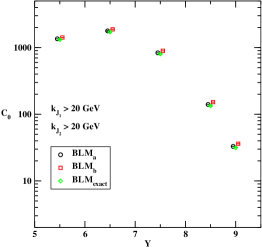
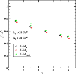
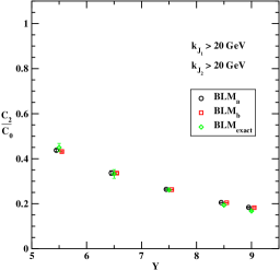
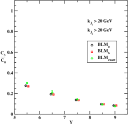
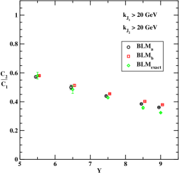
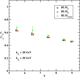
Figure 3.9: $Y$-dependence of $C_{0}$ and of several ratios $C_{m}/C_{n}$ for $k_{J_{1}}^{\rm min}=k_{J_{2}}^{\rm min}=20$ GeV, $|y_{J_{1}}|>2.5$ and for $\sqrt{s}=13$ TeV, from the three variants of the BLM method (data points have been slightly shifted along the horizontal axis for the sake of readability; see Table 3.4).

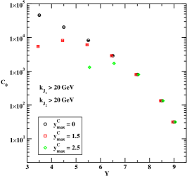
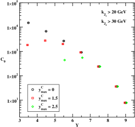
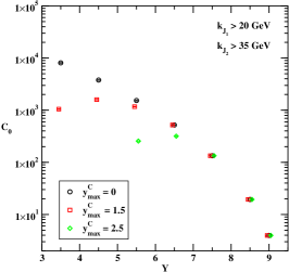
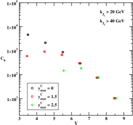
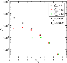
Figure 3.10: $Y$-dependence of $C_{0}$ from the exact BLM method (Eq. 3.7), for all choices of the cuts on jet transverse momenta and of the central rapidity region, and for $\sqrt{s}=13$ TeV (data points have been slightly shifted along the horizontal axis for the sake of readability; see Table 3.5).

We summarise our results in Tables 3.4-3.10 and in Figs. 3.9-3.15. From Table 3.4 (and Fig. 3.9) we can see that the different variants of implementation of the BLM method give predictions which deviate at the level of $\sim 10\$ for $C_{0}$ and at the level of $\sim 5\$ for $R_{10}$, while they basically agree within errors for all other ratios $R_{nm}$. For this reason, all remaining Tables (and Figures) refer to the “exact” BLM case only. Table 3.5 (and Fig. 3.10) show, quite reasonably, that for all choices of the cuts on jet transverse momenta, the larger is $y^{\rm C}_{\rm max}$, the lower is the total cross section $C_{0}$, up the value of $Y$ is reached where the presence of cut of the central rapidity region becomes ineffective. All remaining Tables (and Figures) unanimously show that all ratios $R_{nm}$ remain unaffected by the cut on the central rapidity region, over the entire region of values of $Y$. This is obvious for the values of $Y$ large enough to be insensitive to the very presence of a non-zero $y^{\rm C}_{\rm max}$, but it is unexpectedly true also for the lower values of $Y$.

The latter point means that in our approach, i.e. NLA BFKL with BLM optimisation, the cut on jet central rapidities leads to a proportional reduction of both the total cross section, $C_{0}$, and the other coefficients $C_{1},C_{2},C_{3}$, which parameterise the azimuthal angle distribution. In other words in our approach, the central cut only reduces the value of the total cross section, but does not affect the azimuthal angle distribution of dijets. It would be very interesting to study whether such feature remains true also in other approaches, both within the BFKL approach, but using different ideæ about the inclusion of the physics beyond NLA, and also in other, non-BFKL schemes, like fixed-order DGLAP or approaches using $k_{T}$-factorisation [Catani:1990eg, Collins:1991ty, Gribov:1984tu, Levin:1991ry] for the central jet production.

Table 3.4: $C_{0}$ [nb] and ratios $C_{n}/C_{m}$ for $k_{J_{1}}^{\rm min}=k_{J_{2}}^{\rm min}=20$ GeV, $y^{\rm C}_{\rm max}=2.5$, $\sqrt{s}=13$ TeV, and for the three variants of the BLM method (see Fig. 3.9).

	$Y$	BLM${}_{a}$	BLM${}_{b}$	BLM${}_{\rm exact}$
	5.5	1353.2(5.6)	1413.2(3.2)	1318(16)
	6.5	1778(23)	1877(13)	1720(49)
$C_{0}$	7.5	834.6(2.8)	893.7(2.0)	803.4(6.6)
	8.5	140.06(25)	152.03(18)	133.91(78)
	9.0	32.97(10)	36.16(12)	31.46(20)
	5.5	0.7641(68)	0.7434(37)	0.775(19)
	6.5	0.674(17)	0.6546(87)	0.686(37)
$C_{1}/C_{0}$	7.5	0.6005(44)	0.5775(22)	0.6104(99)
	8.5	0.5339(19)	0.5092(11)	0.5422(64)
	9.0	0.5091(27)	0.4823(23)	0.5174(65)
	5.5	0.4371(52)	0.4315(29)	0.450(18)
	6.5	0.336(11)	0.3357(53)	0.3329(19)
$C_{2}/C_{0}$	7.5	0.2638(27)	0.2625(13)	0.2611(35)
	8.5	0.2052(11)	0.20452(59)	0.1939(49)
	9.0	0.1835(14)	0.1827(11)	0.1674(14)
	5.5	0.2761(45)	0.2691(26)	0.3019(68)
	6.5	0.1934(74)	0.1907(37)	0.210(18)
$C_{3}/C_{0}$	7.5	0.1383(20)	0.13708(80)	0.144(29)
	8.5	0.09796(70)	0.09765(31)	0.095(17)
	9.0	0.08378(90)	0.08361(63)	0.0775(13)
	5.5	0.5721(71)	0.5804(42)	0.580(24)
	6.5	0.499(15)	0.5128(76)	0.484(27)
$C_{2}/C_{1}$	7.5	0.4393(47)	0.4546(19)	0.4278(55)
	8.5	0.3844(21)	0.4017(11)	0.3576(91)
	9.0	0.3605(23)	0.3788(19)	0.3236(27)
	5.5	0.632(13)	0.6236(74)	0.671(26)
	6.5	0.575(25)	0.568(12)	0.634(55)
$C_{3}/C_{2}$	7.5	0.5241(93)	0.5221(32)	0.5509(92)
	8.5	0.4773(41)	0.4775(18)	0.492(16)
	9.0	0.4565(55)	0.4577(29)	0.4627(59)

Table 3.5: Values of $C_{0}$ [nb] from the exact BLM method (Eq. 3.7) at $\sqrt{s}=13$ TeV, for all choices of the cuts on jet transverse momenta and of the central rapidity region (see Fig. 3.10).

$k_{J_{1}}^{\rm min}$	$k_{J_{2}}^{\rm min}$	$Y$	$y^{\rm C}_{\rm max}=0$	$y^{\rm C}_{\rm max}=1.5$	$y^{\rm C}_{\rm max}=2.5$
		3.5	46100(950)	5498(110)	-
		4.5	20410(290)	8200(130)	-
		5.5	8270(130)	6120(110)	1318(16)
20 GeV	20 GeV	6.5	2902(31)	2902(31)	1720(49)
		7.5	803.4(6.6)	803.4(6.6)	803.4(6.6)
		8.5	133.91(78)	133.91(78)	133.91(78)
		9.0	31.46(20)	31.46(20)	31.46(20)
		3.5	15000(270)	1842(27)	-
		4.5	6734(73)	2779(33)	-
		5.5	2701(51)	2030(34)	442.3(3.4)
20 GeV	30 GeV	6.5	919.8(9.2)	919.8(9.2)	555(13)
		7.5	240.8(1.6)	240.8(1.6)	240.8(1.6)
		8.5	36.44(13)	36.44(13)	36.44(13)
		9.0	7.801(53)	7.801(53)	7.801(53)
		3.5	8090(160)	1050(20)	-
		4.5	3793(54)	1598(21)	-
		5.5	1534(26)	1169(16)	256.0(2.1)
20 GeV	35 GeV	6.5	520.6(6.2)	520.6(6.2)	318.5(6.9)
		7.5	134.2(1.1)	134.2(1.1)	134.2(1.1)
		8.5	19.422(98)	19.422(98)	19.422(98)
		9.0	3.9601(23)	3.9601(23)	3.9601(23)
		3.5	4627(86)	595.3(7.3)	-
		4.5	2137(31)	912(10)	-
		5.5	872(13)	668(10)	146.68(94)
20 GeV	40 GeV	6.5	295.4(2.7)	295.4(2.7)	181.6(4.1)
		7.5	74.75(37)	74.75(37)	74.75(37)
		8.5	10.362(30)	10.362(30)	10.362(30)
		9.0	1.9980(45)	1.9980(45)	1.9980(45)
		3.5	4286(36)	544.7(6.0)	-
		4.5	1618(13)	690.9(3.3)	-
		5.5	555.2(4.1)	429.0(3.6)	94.48(13)
35 GeV	35 GeV	6.5	161.8(1.2)	161.8(1.2)	101.5(1.1)
		7.5	35.70(16)	35.70(16)	35.70(16)
		8.5	4.2843(98)	4.2843(98)	4.2843(98)
		9.0	0.7579(23)	0.7579(23)	0.7579(23)

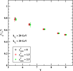
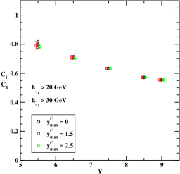
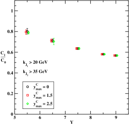
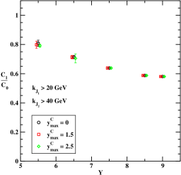
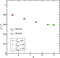
Figure 3.11: $Y$-dependence of $C_{1}/C_{0}$ from the exact BLM method (Eq. 3.7), for all choices of the cuts on jet transverse momenta and of the central rapidity region, and for $\sqrt{s}=13$ TeV (data points have been slightly shifted along the horizontal axis for the sake of readability; see Table 3.6).

Table 3.6: Values of $C_{1}/C_{0}$ from the exact BLM method (Eq. 3.7) at $\sqrt{s}=13$ TeV, for all choices of the cuts on jet transverse momenta and of the central rapidity region (see Fig. 3.11).

$k_{J_{1}}^{\rm min}$	$k_{J_{2}}^{\rm min}$	$Y$	$y^{\rm C}_{\rm max}=0$	$y^{\rm C}_{\rm max}=1.5$	$y^{\rm C}_{\rm max}=2.5$
		3.5	0.988(37)	0.975(35)	-
		4.5	0.885(25)	0.874(27)	-
		5.5	0.785(25)	0.778(31)	0.775(19)
20 GeV	20 GeV	6.5	0.692(18)	0.692(18)	0.686(37)
		7.5	0.6104(99)	0.6104(99)	0.6104(99)
		8.5	0.5423(64)	0.5423(64)	0.5423(64)
		9.0	0.5174(64)	0.5174(64)	0.5174(64)
		3.5	1.004(31)	0.989(28)	-
		4.5	0.896(18)	0.886(20)	-
		5.5	0.799(27)	0.792(27)	0.783(10)
20 GeV	30 GeV	6.5	0.710(13)	0.710(13)	0.702(33
		7.5	0.6321(83)	0.6321(83)	0.6321(83)
		8.5	0.5717(45)	0.5717(45)	0.5717(45)
		9.0	0.5543(70)	0.5543(70)	0.5543(70)
		3.5	1.051(37)	1.005(33)	-
		4.5	0.907(24)	0.892(24)	-
		5.5	0.803(28)	0.795(22)	0.788(13)
20 GeV	35 GeV	6.5	0.712(16)	0.712(16)	0.704(31)
		7.5	0.636(10)	0.636(10)	0.636(10)
		8.5	0.5803(56)	0.5803(56)	0.5803(56)
		9.0	0.5679(74)	0.5679(74)	0.5679(74)
		3.5	1.043(35)	1.021(22)	-
		4.5	0.916(25)	0.899(20)	-
		5.5	0.808(22)	0.798(24)	0.791(10)
20 GeV	40 GeV	6.5	0.714(12)	0.714(12)	0.705(31)
		7.5	0.6383(64)	0.6383(64)	0.6383(64)
		8.5	0.5875(35)	0.5875(35)	0.5875(35)
		9.0	0.5804(25)	0.5804(25)	0.5804(25)
		3.5	0.963(16)	0.952(18)	-
		4.5	0.883(14)	0.8722(82)	-
		5.5	0.798(13)	0.792(12)	0.7866(22)
35 GeV	35 GeV	6.5	0.718(11)	0.718(11)	0.709(16)
		7.5	0.6478(53)	0.6478(53)	0.6478(53)
		8.5	0.5972(26)	0.5972(26)	0.5972(26)
		9.0	0.5886(33)	0.5886(33)	0.5886(33)

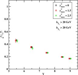
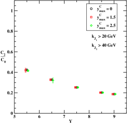
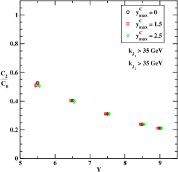
Figure 3.12: $Y$-dependence of $C_{2}/C_{0}$ from the exact BLM method (Eq. 3.7), for all choices of the cuts on jet transverse momenta and of the central rapidity region, and for $\sqrt{s}=13$ TeV (data points have been slightly shifted along the horizontal axis for the sake of readability; see Table 3.7).

Table 3.7: Values of $C_{2}/C_{0}$ from the exact BLM method (Eq. 3.7) at $\sqrt{s}=13$ TeV, for all choices of the cuts on jet transverse momenta and of the central rapidity region (see Fig. 3.12).

$k_{J_{1}}^{\rm min}$	$k_{J_{2}}^{\rm min}$	$Y$	$y^{\rm C}_{\rm max}=0$	$y^{\rm C}_{\rm max}=1.5$	$y^{\rm C}_{\rm max}=2.5$
		3.5	0.749(25)	0.730(30)	-
		4.5	0.594(23)	0.581(24)	-
		5.5	0.458(13)	0.454(27)	0.450(18)
20 GeV	20 GeV	6.5	0.350(13)	0.350(13)	0.332(19)
		7.5	0.2611(35)	0.2611(35)	0.2611(35)
		8.5	0.1939(49)	0.1939(49)	0.1939(49)
		9.0	0.1674(14)	0.1674(14)	0.1674(14)
		3.5	0.727(27)	0.719(26)	-
		4.5	0.575(15)	0.565(17)	-
		5.5	0.450(20)	0.443(21)	0.4398(98)
20 GeV	30 GeV	6.5	0.3483(94)	0.3483(94)	0.343(24)
		7.5	0.2683(53)	0.2683(53)	0.2683(53)
		8.5	0.2083(30)	0.2083(30)	0.2083(30)
		9.0	0.1872(39)	0.1872(39)	0.1872(39)
		3.5	0.750(22)	0.714(29)	-
		4.5	0.563(20)	0.555(20)	-
		5.5	0.435(11)	0.430(17)	0.4268(40)
20 GeV	35 GeV	6.5	0.337(12)	0.337(12)	0.331(20)
		7.5	0.2602(32)	0.2602(32)	0.2602(32)
		8.5	0.2059(37)	0.2059(37)	0.2059(37)
		9.0	0.1874(15)	0.1874(15)	0.1874(15)
		3.5	0.727(21)	0.710(19)	-
		4.5	0.560(17)	0.546(16)	-
		5.5	0.4225(99)	0.420(20)	0.4158(75)
20 GeV	40 GeV	6.5	0.3276(91)	0.3276(91)	0.321(23)
		7.5	0.2528(22)	0.2528(22)	0.2528(22)
		8.5	0.2021(26)	0.2021(26)	0.2021(26)
		9.0	0.18712(7)	0.18712(7)	0.18712(7)
		3.5	0.778(16)	0.766(16)	-
		4.5	0.642(12)	0.6321(85)	-
		5.5	0.5260(94)	0.510(12)	0.5051(20)
35 GeV	35 GeV	6.5	0.4038(86)	0.4038(86)	0.398(13)
		7.5	0.3109(45)	0.3109(45)	0.3109(45)
		8.5	0.2379(25)	0.2379(25)	0.2379(25)
		9.0	0.2112(37)	0.2112(37)	0.2112(37)

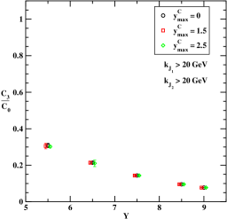
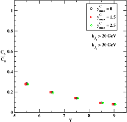
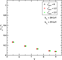
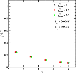
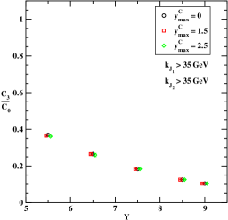
Figure 3.13: $Y$-dependence of $C_{3}/C_{0}$ from the exact BLM method (Eq. 3.7), for all choices of the cuts on jet transverse momenta and of the central rapidity region, and for $\sqrt{s}=13$ TeV (data points have been slightly shifted along the horizontal axis for the sake of readability; see Table 3.8).

Table 3.8: Values of $C_{3}/C_{0}$ from the exact BLM method (Eq. 3.7) at $\sqrt{s}=13$ TeV, for all choices of the cuts on jet transverse momenta and of the central rapidity region (see Fig. 3.13).

$k_{J_{1}}^{\rm min}$	$k_{J_{2}}^{\rm min}$	$Y$	$y^{\rm C}_{\rm max}=0$	$y^{\rm C}_{\rm max}=1.5$	$y^{\rm C}_{\rm max}=2.5$
		3.5	0.593(22)	0.577(19)	-
		4.5	0.432(13)	0.425(14)	-
		5.5	0.308(12)	0.305(15)	0.3019(68)
20 GeV	20 GeV	6.5	0.2139(67)	0.2139(67)	0.210(18)
		7.5	0.1439(29)	0.1439(29)	0.1439(29)
		8.5	0.0954(17)	0.0954(17)	0.0954(17)
		9.0	0.0775(13)	0.0775(13)	0.0775(13)
		3.5	0.551(26)	0.544(14)	-
		4.5	0.3950(88)	0.3896(97)	-
		5.5	0.281(13)	0.278(12)	0.276(3)
20 GeV	30 GeV	6.5	0.1973(48)	0.1973(48)	0.194(14)
		7.5	0.1389(49)	0.1389(49)	0.1389(49)
		8.5	0.0944(13)	0.0944(13)	0.0944(13)
		9.0	0.0795(25)	0.0795(25)	0.0795(25)
		3.5	0.555(19)	0.528(15)	-
		4.5	0.377(11)	0.3724(94)	-
		5.5	0.2652(90)	0.263(10)	0.2599(30)
20 GeV	35 GeV	6.5	0.1842(48)	0.1842(48)	0.184(11)
		7.5	0.1272(24)	0.1272(24)	0.1272(24)
		8.5	0.0888(11)	0.0888(11)	0.0888(11)
		9.0	0.0756(12)	0.0756(12)	0.0756(12)
		3.5	0.529(18)	0.520(21)	-
		4.5	0.364(10)	0.3585(79)	-
		5.5	0.2496(80)	0.249(11)	0.2400(40)
20 GeV	40 GeV	6.5	0.1717(41)	0.1717(41)	0.171(13)
		7.5	0.1188(18)	0.1188(18)	0.1188(18)
		8.5	0.0836(66)	0.0836(66)	0.0836(66)
		9.0	0.0720(52)	0.0720(52)	0.0720(52)
		3.5	0.6478(76)	0.6360(95)	-
		4.5	0.4983(75)	0.4887(40)	-
		5.5	0.3690(55)	0.3652(69)	0.3613(84)
35 GeV	35 GeV	6.5	0.2648(47)	0.2648(47)	0.2596(93)
		7.5	0.1838(17)	0.1838(17)	0.1838(17)
		8.5	0.1257(16)	0.1257(16)	0.1257(16)
		9.0	0.1043(12)	0.1043(12)	0.1043(12)

Table 3.9: Values of $C_{2}/C_{1}$ from the exact BLM method (Eq. 3.7) at $\sqrt{s}=13$ TeV, for all choices of the cuts on jet transverse momenta and of the central rapidity region (see Fig. 3.14).

$k_{J_{1}}^{\rm min}$	$k_{J_{2}}^{\rm min}$	$Y$	$y^{\rm C}_{\rm max}=0$	$y^{\rm C}_{\rm max}=1.5$	$y^{\rm C}_{\rm max}=2.5$
		3.5	0.759(21)	0.749(28)	-
		4.5	0.671(26)	0.665(28)	-
		5.5	0.583(17)	0.583(37)	0.580(24)
20 GeV	20 GeV	6.5	0.506(21)	0.506(21)	0.484(27)
		7.5	0.4278(55)	0.4278(55)	0.4278(55)
		8.5	0.3576(91)	0.3576(91)	0.3576(91)
		9.0	0.3236(27)	0.3236(27)	0.3236(27)
		3.5	0.724(23)	0.727(25)	-
		4.5	0.642(15)	0.638(18)	-
		5.5	0.563(23)	0.559(27)	0.561(11)
20 GeV	30 GeV	6.5	0.491(13)	0.491(13)	0.489(34)
		7.5	0.4245(83)	0.4245(83)	0.4245(83)
		8.5	0.3644(54)	0.3644(54)	0.3644(54)
		9.0	0.3377(67)	0.3377(67)	0.3377(67)
		3.5	0.713(19)	0.710(24)	-
		4.5	0.622(21)	0.623(22)	-
		5.5	0.542(14)	0.542(22)	0.5414(50)
20 GeV	35 GeV	6.5	0.473(17)	0.473(17)	0.470(29)
		7.5	0.4095(50)	0.4095(50)	0.4095(50)
		8.5	0.3548(63)	0.3548(63)	0.3548(63)
		9.0	0.3299(31)	0.3299(31)	0.3299(31)
		3.5	0.697(18)	0.695(16)	-
		4.5	0.612(17)	0.607(17)	-
		5.5	0.523(10)	0.526(24)	0.5256(96)
20 GeV	40 GeV	6.5	0.459(12)	0.459(12)	0.455(33)
		7.5	0.3960(33)	0.3960(33)	0.3960(33)
		8.5	0.3441(45)	0.3441(45)	0.3441(45)
		9.0	0.3224(12)	0.3224(12)	0.3224(12)
		3.5	0.809(16)	0.805(14)	-
		4.5	0.728(14)	0.7247(98)	-
		5.5	0.659(13)	0.644(14)	0.6421(27)
35 GeV	35 GeV	6.5	0.562(12)	0.563(12)	0.561(19)
		7.5	0.4799(67)	0.4799(67)	0.4799(67)
		8.5	0.3984(40)	0.3984(40)	0.3984(40)
		9.0	0.3588(61)	0.3588(61)	0.3588(61)

Table 3.10: Values of $C_{3}/C_{2}$ from the exact BLM method (Eq. 3.7) at $\sqrt{s}=13$ TeV, for all choices of the cuts on jet transverse momenta and of the central rapidity region (see Fig. 3.15).

$k_{J_{1}}^{\rm min}$	$k_{J_{2}}^{\rm min}$	$Y$	$y^{\rm C}_{\rm max}=0$	$y^{\rm C}_{\rm max}=1.5$	$y^{\rm C}_{\rm max}=2.5$
		3.5	0.792(22)	0.790(26)	-
		4.5	0.727(30)	0.731(32)	-
		5.5	0.673(24)	0.672(49)	0.671(26)
20 GeV	20 GeV	6.5	0.611(28)	0.611(28)	0.634(55)
		7.5	0.5509(92)	0.5509(92)	0.5509(92)
		8.5	0.492(16)	0.492(16)	0.492(16)
		9.0	0.4627(59)	0.4627(59)	0.4627(59)
		3.5	0.758(37)	0.756(23)	-
		4.5	0.687(18)	0.689(22)	-
		5.5	0.625(32)	0.629(36)	0.628(11)
20 GeV	30 GeV	6.5	0.566(18)	0.567(18)	0.566(54)
		7.5	0.518(22)	0.518(22)	0.518(22)
		8.5	0.4530(93)	0.4530(93)	0.4530(93)
		9.0	0.424(17)	0.424(17)	0.424(17)
		3.5	0.741(19)	0.740(23)	-
		4.5	0.670(24)	0.671(23)	-
		5.5	0.609(15)	0.610(32)	0.6090(25)
20 GeV	35 GeV	6.5	0.547(21)	0.547(21)	0.555(43)
		7.5	0.4887(75)	0.4887(75)	0.4887(75)
		8.5	0.4312(86)	0.4312(86)	0.4312(86)
		9.0	0.4033(50)	0.4033(50)	0.4033(50)
		3.5	0.728(19)	0.732(32)	-
		4.5	0.650(18)	0.657(18)	-
		5.5	0.591(15)	0.592(34)	0.578(13)
20 GeV	40 GeV	6.5	0.524(17)	0.524(17)	0.532(56)
		7.5	0.4700(63)	0.4700(63)	0.4700(63)
		8.5	0.4134(62)	0.4134(62)	0.4134(62)
		9.0	0.3850(25)	0.3850(25)	0.3850(25)
		3.5	0.832(13)	0.830(11)	-
		4.5	0.776(14)	0.7731(94)	-
		5.5	0.701(13)	0.716(18)	0.7152(27)
35 GeV	35 GeV	6.5	0.656(16)	0.656(16)	0.652(31)
		7.5	0.5912(88)	0.5912(88)	0.5912(88)
		8.5	0.5284(96)	0.5284(96)	0.5284(96)
		9.0	0.4939(11)	0.4939(11)	0.4939(11)

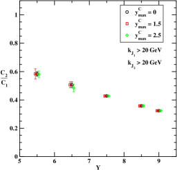
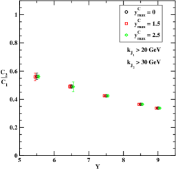
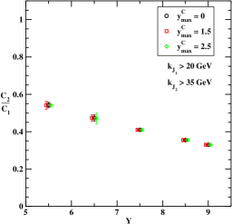
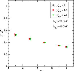
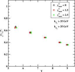
Figure 3.14: $Y$-dependence of $C_{2}/C_{1}$ from the exact BLM method (Eq. 3.7), for all choices of the cuts on jet transverse momenta and of the central rapidity region, and for $\sqrt{s}=13$ TeV (data points have been slightly shifted along the horizontal axis for the sake of readability; see Table 3.9).

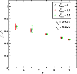
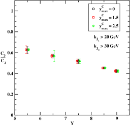
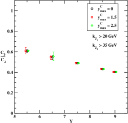
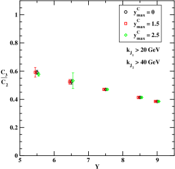
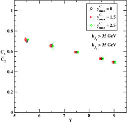
Figure 3.15: $Y$-dependence of $C_{3}/C_{2}$ from the exact BLM method (Eq. 3.7), for all choices of the cuts on jet transverse momenta and of the central rapidity region, and for $\sqrt{s}=13$ TeV (data points have been slightly shifted along the horizontal axis for the sake of readability; see Table 3.10).

3.5 Numerical specifics

In this Section the numerical specifics for all the calculations done in Sections 3.3 and 3.4 are discussed.

3.5.1 Used tools

All numerical calculations were implemented in Fortran, using the corresponding interfaces for the NLO MSTW 2008 PDFs [Martin:2009iq] and the two-loop running coupling with $\alpha_{s}\left(M_{Z}\right)=0.11707$ with five quark flavours active. Now there exist updated PDF parameterisations, including the NLO MMHT 2014 set [Harland-Lang:2014zoa], which is the successor of the MSTW 2008 analysis. Here we continue to use MSTW 2008 PDFs because in our kinematical range the difference between MSTW 2008 and the updated MMHT 2014 PDFs is very small. Also, we want to keep the opportunity to compare our results at 13 TeV with our previous calculations at 7 TeV without introducing any other source of discrepancy related to the change of the PDF set. Numerical integrations and the computation of the polygamma functions were performed using specific CERN program libraries [cernlib]. Furthermore, we used slightly modified versions of the Chyp [chyp] and Psi [RpsiCody:1973] routines in order to perform the calculation of the Gauss hypergeometric function ${}_{2}F_{1}$ and of the real part of the $\psi$ function, respectively.

3.5.2 Uncertainty estimation

The are three main sources of uncertainty in our calculation:

• The first source of uncertainty is the numerical 4-dimensional integration over the variables $|\vec{k}_{J_{1}}|$, $|\vec{k}_{J_{2}}|$, $y_{J_{1}}$ and $\nu$ and was directly estimated by Dadmul integration routine [cernlib].

• The second one is the one-dimensional integration over the longitudinal momentum fraction $\zeta$ entering the expression for the NLO impact factors $c_{1,2}^{(1)}(n,\nu,|\vec{k}_{J_{1,2}}|,x_{J_{1,2}})$ (see Appendix B). This integration was performed by using the WGauss routine [cernlib]. At first, we fixed the best value of the input accuracy parameter EPS by making comparisons between separate Fortran and Mathematica calculations of the impact factor. Then, we verified that, under variations by factors of 10 or 1/10 of the EPS parameter, the $C_{n}^{\rm BFKL}$ and $C_{n}^{\rm DGLAP}$ coefficients change by less than 1 permille.

• The third one is related to the upper cutoff in the integrations over $|\vec{k}_{J_{1}}|$, $|\vec{k}_{J_{2}}|$ and $\nu$. We fixed $k_{J_{1}}^{\rm max}=k_{J_{2}}^{\rm max}=60$ GeV as in Ref. [Ducloue:2013wmi], where it was shown that the contribution to the integration from the omitted region is negligible. Concerning the $\nu$-integration, we fixed the upper cutoff $\nu^{\rm max}=30$ for the calculation of the $C_{n}^{\rm BFKL}$ coefficients, after verifying that a larger value does not change the result in appreciable way.

  The $C_{n}^{\rm DGLAP}$ coefficients show a more pronounced sensitivity to $\nu^{\rm max}$, due to the fact that the oscillations in the integrand in Eqs. (3.11) and (3.13) are not dumped by the exponential factor as in the BFKL expressions (2.85) and (2.87). For the same reason, the computational time of $C_{n}^{\rm DGLAP}$ is much larger than for $C_{n}^{\rm BFKL}$. We found that the best compromise was to set $\nu^{\rm max}=50$. We checked in some sample cases, mostly at $Y=6$ and 9, that, putting $\nu^{\rm max}$ at 60, ratios $C_{m}/C_{n}$ change always less than 1%, in spite of the fact that the single coefficients $C_{n}$ change in a more pronounced way.

Of the three main sources of uncertainty, the first one is, by far, the most significant, therefore the error bars of all data presented in this work are just those given by the Dadmul integration. We checked, however, using some trial functions which mimic the behaviour of the true integrands involved in this work, that the error given by the Dadmul integration is a large overestimate of the true one. We are therefore confident that our error estimation is quite conservative.

3.6 Summary

In this Chapter we have considered the Mueller–Navelet jet production process at the LHC at the two values for center-of-mass energy of $7$ TeV and $13$ TeV and for several and distinct kinematical configurations for the transverse momenta of the detected jets.

First, we have shown how BFKL predictions [Caporale:2014gpa] taken at $\sqrt{s}=7$ TeV, for symmetric cuts for the transverse momenta ($k_{J_{1,2}\rm\,min}=35$ GeV) and with the renormalisation and the factorization scales optimised according to the BLM method, are in a very good agreement with experimental data [Khachatryan:2016udy]. Then, we have addressed some of the open questions raised in recent phenomenological works (see Section 3.2).

On one side [Celiberto:2015yba], we compared predictions for several azimuthal correlations and ratios between them at $\sqrt{s}=7$ TeV, both in full NLA BFKL approach and in fixed-order NLO DGLAP. Differently from current experimental analyses of the same process, we have used asymmetric cuts for the transverse momenta of the detected jets. In particular, taking one of the cuts at 35 GeV (as done by the CMS collaboration [Khachatryan:2016udy]) and the other at 45 GeV or 50 GeV, we can clearly see that predictions from BFKL and DGLAP become separate for most azimuthal correlations and ratios between them, this effect being more and more visible as the rapidity gap between the jets, $Y$, increases. In other words, in this kinematics the additional undetected parton radiation between the jets which is present in the resummed BFKL series, in comparison to just one undetected parton allowed by the NLO DGLAP approach, makes its difference and leads to more azimuthal angle decorrelation between the jets, in full agreement with the original proposal of Mueller and Navelet. Another important benefit from the use of asymmetric cuts, pointed out in [Ducloue:2014koa], is that the effect of violation of the energy-momentum conservation in the NLA is strongly suppressed with respect to what happens in the LLA. All these considerations persuade us to strongly suggest experimental collaborations to consider also asymmetric cuts in jet transverse momenta in all future analyses of Mueller–Navelet jet production process.

On the other side [Celiberto:2016ygs], we performed the first analysis at $\sqrt{s}=13$ TeV, studying the jet azimuthal correlations in five different configurations for the jet transverse momenta, which include asymmetric cuts. Differently from all previous studies of the same kind, we considered in our analysis the effect of excluding the possibility that one of the two detected jets be produced in the central rapidity region. Central jets originate from small-$x$ partons, and the collinear approach for the description of the Mueller–Navelet jet vertices may not hold at small $x$. The outcome of our analysis is that, for two reasonable ways to define the extension of the central region: $(i)$ the total cross section, $C_{0}$, is strongly reduced by the “exclusion cuts” in the range ($Y<5.5$) where they are effective; $(ii)$ on the other hand, in the same kinematics, the difference with respect to the case of no central rapidity exclusion is invisible in azimuthal correlations and in ratios between them. We believe that it would be very interesting to confront these conclusions with the forthcoming LHC analysis at $13$ TeV.

As anticipated in Section 2.3.3, it would be interesting to figure out whether the growth with energy of the cross section, a characteristic feature of the BFKL resummation, can be observed in the Mueller–Navelet jet reaction. First of all, the relevant observable for such investigation is the $\phi$-averaged cross section ${\cal C}_{0}$, which, however, is affected by theoretical ambiguities coming from the choice of the representation (see Section 2.3.3.1) and the scale setting procedure (see Section 2.4). The possible experimental measurement of ${\cal C}_{0}$ would be extremely helpful in discriminating among the several NLA-equivalent options. Even in case the theoretical ambiguities in the definition of ${\cal C}_{0}$ were cleared up, the search for the growth in the jet rapidity interval $Y$ of the cross section and the subsequent extraction of the Pomeron intercept would be hindered by the fact that, due to collinear factorisation, the hadronic cross section embeds the parent proton PDFs which are responsible of its decrease for increasing $Y$. To switch off the role of PDFs and thus isolate the $Y$-dependence of the partonic cross section, one should select final-state configurations so as to keep $x$ constant in the PDFs. The price for that, however, is a too restrictive choice of the ranges for the jet transverse momenta. Indeed, since the dependence of $x$ on the rapiditity is exponential (Eq. (3.6)), one should consider ranges for the transverse momenta which are much larger than the ones available at the present and forthcoming LHC energies. Furthermore, there is a principle difficulty in detecting at the LHC clear imprints of a genuine BFKL power asymptotic. As already stated at the end of Section 3.3.2, the limited number of undetected hard partons emitted with LHC kinematics makes BFKL hardly distinguishable from DGLAP when one goes from LLA to NLA, so that it is difficult to say something definite about the intercept. We can only compare our predictions for the cross section with data, to see whether our approach in its present status works or not. Although these issues affect also the other hadroproduction processes investigated in this thesis, dihadron production (see Chapter 4) has better chances to bring us closer to the Regge kinematics for partonic subprocesses, due to the fact that hadrons can be detected at the LHC at much smaller transverse momenta than jets.

Appendix B

NLO impact factor for the small-cone forward jet

In this Appendix the expression for the NLO correction to the forward jet impact factor in the small-cone limit is given (see Ref. [Caporale:2012ih] for further details). In the $(\nu,n)$ representation, we have:

$$c_{1}^{(1)}(n,\nu,|\vec{k}|,x)=\frac{1}{\pi}\sqrt{\frac{C_{F}}{C_{A}}}\left(\vec{k}^{\,2}\right)^{i\nu-1/2}\int\limits^{1}_{x}\frac{d\zeta}{\zeta}\zeta^{-\bar{\alpha}_{s}(\mu_{R})\chi(n,\nu)}$$ (B.1)

$$\left\{\sum_{a=q,\bar{q}}f_{a}\left(\frac{x}{\zeta}\right)\left[\left(P_{qq}(\zeta)+\frac{C_{A}}{C_{F}}P_{gq}(\zeta)\right)\ln\frac{\vec{k}^{\,2}}{\mu_{F}^{2}}\right.\right.$$

$$-2\zeta^{-2\gamma}\ln R\,\left\{P_{qq}(\zeta)+P_{gq}(\zeta)\right\}-\frac{\beta_{0}}{2}\ln\frac{\vec{k}^{\,2}}{\mu_{R}^{2}}\delta(1-\zeta)$$

$$+C_{A}\delta(1-\zeta)\left(\chi(n,\gamma)\ln\frac{s_{0}}{\vec{k}^{\,2}}+\frac{85}{18}+\frac{\pi^{2}}{2}\right.$$

$$\left.+\frac{1}{2}\left(\psi^{\prime}\left(1+\gamma+\frac{n}{2}\right)-\psi^{\prime}\left(\frac{n}{2}-\gamma\right)-\chi^{2}(n,\gamma)\right)\right)$$

$$+(1+\zeta^{2})\left\{C_{A}\left(\frac{(1+\zeta^{-2\gamma})\,\chi(n,\gamma)}{2(1-\zeta)_{+}}-\zeta^{-2\gamma}\left(\frac{\ln(1-\zeta)}{1-\zeta}\right)_{+}\right)\right.$$

$$\left.+\left(C_{F}-\frac{C_{A}}{2}\right)\left[\frac{\bar{\zeta}}{\zeta^{2}}I_{2}-\frac{2\ln\zeta}{1-\zeta}+2\left(\frac{\ln(1-\zeta)}{1-\zeta}\right)_{+}\right]\right\}$$

$$+\delta(1-\zeta)\left(C_{F}\left(3\ln 2-\frac{\pi^{2}}{3}-\frac{9}{2}\right)-\frac{5n_{f}}{9}\right)+C_{A}\zeta+C_{F}\bar{\zeta}$$

$$\left.+\frac{1+\bar{\zeta}^{2}}{\zeta}\left(C_{A}\frac{\bar{\zeta}}{\zeta}I_{1}+2C_{A}\ln\frac{\bar{\zeta}}{\zeta}+C_{F}\zeta^{-2\gamma}(\chi(n,\gamma)-2\ln\bar{\zeta})\right)\right]$$

$$+f_{g}\left(\frac{x}{\zeta}\right)\frac{C_{A}}{C_{F}}\left[\left(P_{gg}(\zeta)+2\,n_{f}\frac{C_{F}}{C_{A}}P_{qg}(\zeta)\right)\ln\frac{\vec{k}^{\,2}}{\mu_{F}^{2}}\right.$$

$$\left.-2\zeta^{-2\gamma}\ln R\left(P_{gg}(\zeta)+2\,n_{f}P_{qg}(\zeta)\right)-\frac{\beta_{0}}{2}\ln\frac{\vec{k}^{\,2}}{4\mu_{R}^{2}}\delta(1-\zeta)\right.$$

$$+\,C_{A}\delta(1-\zeta)\left(\chi(n,\gamma)\ln\frac{s_{0}}{\vec{k}^{\,2}}+\frac{1}{12}+\frac{\pi^{2}}{6}\right.$$

$$\left.+\frac{1}{2}\left(\psi^{\prime}\left(1+\gamma+\frac{n}{2}\right)-\psi^{\prime}\left(\frac{n}{2}-\gamma\right)-\chi^{2}(n,\gamma)\right)\right)$$

$$+\,2C_{A}(1-\zeta^{-2\gamma})\left(\left(\frac{1}{\zeta}-2+\zeta\bar{\zeta}\right)\ln\bar{\zeta}+\frac{\ln(1-\zeta)}{1-\zeta}\right)$$

$$+\,C_{A}\,\left[\frac{1}{\zeta}+\frac{1}{(1-\zeta)_{+}}-2+\zeta\bar{\zeta}\right]\left((1+\zeta^{-2\gamma})\chi(n,\gamma)-2\ln\zeta+\frac{\bar{\zeta}^{2}}{\zeta^{2}}I_{2}\right)$$

$$\left.\left.+\,n_{f}\left[\,2\zeta\bar{\zeta}\,\frac{C_{F}}{C_{A}}+(\zeta^{2}+\bar{\zeta}^{2})\left(\frac{C_{F}}{C_{A}}\chi(n,\gamma)+\frac{\bar{\zeta}}{\zeta}I_{3}\right)-\frac{1}{12}\delta(1-\zeta)\right]\right]\right\}\;.$$

Here $\bar{\zeta}=1-\zeta$, $\gamma=i\nu-1/2$, $P_{ij}(\zeta)$ are leading order DGLAP kernels defined as

$$P_{gq}(z) = C_{F}\frac{1+(1-z)^{2}}{z}\;,$$ (B.2)

$$P_{qg}(z) = T_{R}\left[z^{2}+(1-z)^{2}\right]\;,$$

$$P_{qq}(z) = C_{F}\left(\frac{1+z^{2}}{1-z}\right)_{+}=C_{F}\left[\frac{1+z^{2}}{(1-z)_{+}}+{3\over 2}\delta(1-z)\right]\;,$$

$$P_{gg}(z) = 2C_{A}\left[\frac{1}{(1-z)_{+}}+\frac{1}{z}-2+z(1-z)\right]+\left({11\over 6}C_{A}-\frac{n_{f}}{3}\right)\delta(1-z)\;,$$

where $C_{F}$ is the Casimir operator associated with gluon emission from a quark, $C_{F}=(N_{c}^{2}-1)/(2N_{c})$ and $T_{R}=1/2$ is the colour factor associated with the splitting of a gluon into a quark-antiquark pair. For the $I_{1,2,3}$ functions we have the results:

$$I_{2}=\frac{\zeta^{2}}{\bar{\zeta}^{2}}\left[\zeta\left(\frac{{}_{2}F_{1}(1,1+\gamma-\frac{n}{2},2+\gamma-\frac{n}{2},\zeta)}{\frac{n}{2}-\gamma-1}-\frac{{}_{2}F_{1}(1,1+\gamma+\frac{n}{2},2+\gamma+\frac{n}{2},\zeta)}{\frac{n}{2}+\gamma+1}\right)\right.$$

$$\left.+\zeta^{-2\gamma}\left(\frac{{}_{2}F_{1}(1,-\gamma-\frac{n}{2},1-\gamma-\frac{n}{2},\zeta)}{\frac{n}{2}+\gamma}-\frac{{}_{2}F_{1}(1,-\gamma+\frac{n}{2},1-\gamma+\frac{n}{2},\zeta)}{\frac{n}{2}-\gamma}\right)\right.$$ (B.3)

$$\left.+\left(1+\zeta^{-2\gamma}\right)\left(\chi(n,\gamma)-2\ln\bar{\zeta}\right)+2\ln{\zeta}\right]\;,$$

$$I_{1}=\frac{\bar{\zeta}}{2\zeta}I_{2}+\frac{\zeta}{\bar{\zeta}}\left[\ln\zeta+\frac{1-\zeta^{-2\gamma}}{2}\left(\chi(n,\gamma)-2\ln\bar{\zeta}\right)\right]\;,$$ (B.4)

$$I_{3}=\frac{\bar{\zeta}}{2\zeta}I_{2}-\frac{\zeta}{\bar{\zeta}}\left[\ln\zeta+\frac{1-\zeta^{-2\gamma}}{2}\left(\chi(n,\gamma)-2\ln\bar{\zeta}\right)\right]\;.$$ (B.5)

In Eq. (B.1) the plus-prescription is introduced, which is defined as

$$\int\limits^{1}_{a}d\zeta\frac{F(\zeta)}{(1-\zeta)_{+}}=\int\limits^{1}_{a}d\zeta\frac{F(\zeta)-F(1)}{(1-\zeta)}-\int\limits^{a}_{0}d\zeta\frac{F(1)}{(1-\zeta)}\;,$$ (B.6)

for any function $F(\zeta)$, regular at $\zeta=1$. Note that

$$(1-\zeta)^{2\epsilon-1}=(1-\zeta)^{2\epsilon-1}_{+}+\frac{1}{2\epsilon}\delta(1-\zeta)$$ (B.7)

$$=\frac{1}{2\epsilon}\delta(1-\zeta)+\frac{1}{(1-\zeta)_{+}}+2\epsilon\left(\frac{\ln(1-\zeta)}{1-\zeta}\right)_{+}+{\cal O}(\epsilon^{2})\;.$$

The factor $\zeta^{-\bar{\alpha}_{s}(\mu_{R})\chi(n,\nu)}$ appears in Eq. (B.1) due to extra contributions attributed to the jet vertices, as discussed after Eq. (29) of Ref. [Caporale:2012ih].

Chapter 4 Dihadron production

In this Chapter the inclusive dihadron production

$${\rm p}(p_{1})+{\rm p}(p_{2})\to{\rm h}_{1}(k_{1})+{\rm h}_{2}(k_{2})+{\rm X}$$ (4.1)

is investigated, i.e. when the two charged light hadrons: $\pi^{\pm},K^{\pm},p,\bar{p}$ with high transverse momenta and separated by a large interval of rapidity, together with an undetected hadronic system X, are produced in the final state (see Fig. 4.1 for a schematic view).

This process is similar to the Mueller–Navelet jet production and shares with it the underlying theoretical framework, the only obvious difference lying in the vertices describing the dynamics in the proton fragmentation region: instead of the proton-to-jet vertex, the vertex for the proton to identified hadron transition is needed. Such a vertex was considered in [hadrons] within NLA: it was shown there that ultraviolet divergences are taken care of by the renormalisation of the QCD coupling, soft and virtual infrared divergences cancel each other, whereas the surviving infrared collinear ones are compensated by the collinear counterterms related to the renormalisation of PDFs for the initial proton and FFs describing the detected hadron in the final state within collinear factorisation. Hence, infrared-safe NLA predictions for observables related to this process are amenable, thus making this process an additional clear channel to test the BFKL dynamics at the LHC. The reaction (4.1) can be considered complementary to Mueller–Navelet jet production, since hadrons can be detected at the LHC at much smaller values of the transverse momentum than jets, thus giving access to a kinematical range outside the reach of the Mueller–Navelet channel.

This Chapter is organised as follows. In Section 4.1 we give the main formulæ for cross section and azimuthal correlations (see Section 4.1.2), together with the BLM scale setting (see Section 4.1.4) and the final-state phase space integration (see Section 4.1.3). In Section 4.2 we present a comparison between full LLA and partial NLA BFKL predictions, i.e. considering just the NLO kernel corrections and taking the hadron vertices at LLA. Full NLA predictions at 7 and 13 TeV and considering various realistic LHC kinematical constraint are given in Section 4.3. Section 4.4 is devoted to the details on the numerical implementation, together with the study of the effects of using different PDF and FF parameterisations. The section Summary is drawn in Section 4.5.

The analysis given in this Chapter is based on the work done in Refs. [Celiberto:2016hae, Celiberto:2017ptm] and presented in Refs. [Celiberto:2016vhn, Celiberto:2016zgb, Celiberto:2017:lowx, Celiberto:2017:blois].

4.1 Theoretical framework

In this Section the BFKL cross section and the azimuthal corrections for the inclusive dihadron production process are presented.

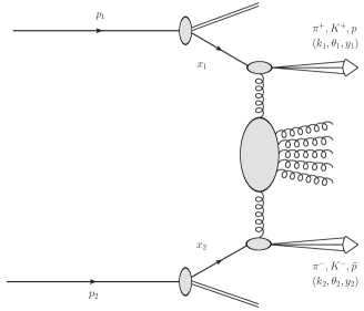
Figure 4.1: Inclusive dihadron production process in multi-Regge kinematics.

4.1.1 Inclusive dihadron production

The process under investigation (see Eq. (4.1) and Fig. 4.1) is the inclusive production of a pair of identified hadrons featuring high transverse momenta, $\vec{k}_{1}^{2}\sim\vec{k}_{2}^{2}\gg\Lambda^{2}_{\rm QCD}$ and separated by a large rapidity interval in high-energy proton-proton collisions. The protons’ momenta $p_{1}$ and $p_{2}$ are taken as Sudakov vectors (see Eq. (2.10)) satisfying $p^{2}_{1}=p^{2}_{2}=0$ and $2(p_{1}p_{2})=s$, so that the momentum of each hadron can be decomposed as

$$k_{1} = \alpha_{1}p_{1}+\frac{\vec{k}_{1}^{2}}{\alpha_{1}s}p_{2}+k_{1\perp}\ ,\quad k_{1\perp}^{2}=-\vec{k}_{1}^{2}\ ,$$ (4.2)

$$k_{2} = \alpha_{2}p_{2}+\frac{\vec{k}_{2}^{2}}{\alpha_{2}s}p_{1}+k_{2\perp}\ ,\quad k_{2\perp}^{2}=-\vec{k}_{2}^{2}\ .$$

In the center of mass system, the hadrons’ longitudinal momentum fractions $\alpha_{1,2}$ are connected to the respective rapidities through the relations $y_{1}=\frac{1}{2}\ln\frac{\alpha_{1}^{2}s}{\vec{k}_{1}^{2}}$, and $y_{2}=\frac{1}{2}\ln\frac{\vec{k}_{2}^{2}}{\alpha_{2}^{2}s}$, so that $dy_{1}=\frac{d\alpha_{1}}{\alpha_{1}}$, $dy_{2}=-\frac{d\alpha_{2}}{\alpha_{2}}$, and $Y=y_{1}-y_{2}=\ln\frac{\alpha_{1}\alpha_{2}s}{|\vec{k}_{1}||\vec{k}_{2}|}$, here the space part of the four-vector $p_{1\parallel}$ being taken positive.

By studying Mueller–Navelet jets, we probed the BFKL dynamics through a very inclusive process. Now we require that a couple of hadrons is always identified in the final state, considering so a less inclusive final-state reaction. Following the course taken in the Mueller–Navelet case (see Section 3.1.1), we start from the NLO forward parton impact factors [Fadin:1999de, Fadin:1999df] (see Fig. 3.2). In order to allow the inclusive production of a given hadron, one of these integrations in the definition of parton impact factors is ‘opened’ (see Fig. 3.2). This means that the integration over the momentum of one of the intermediate-state partons is replaced by the convolution with a suitable FF.

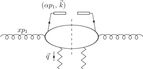
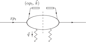
Figure 4.2: Schematic view of the the vertex for the identified hadron production for the case of incoming gluon (left) or quark (right). Here $p_{1}$ is the proton momentum, $x$ is the fraction of proton momentum carried by the gluon/quark, $\alpha_{h}p_{1}$ is the longitudinal momentum of the hadron $h$, $\vec{k}_{h}$ is the transverse hadron momentum and $\vec{q}$ is the transverse momentum of the incoming Reggeised gluon.

The expression for the identified-hadron impact factor with LO accuracy is given below (see Fig. 4.2):

$$\frac{d\Phi_{h}^{(0)}}{\vec{q}^{2}}=2\pi\alpha_{s}\sqrt{\frac{2C_{F}}{C_{A}}}\frac{d\alpha_{h}d^{2}\vec{k}}{\vec{k}^{\,2}}\int\limits^{1}_{\alpha_{h}}\frac{dx}{x}\,\delta^{(2)}\left(\vec{k}-\vec{q}\right)$$ (4.3)

$$\times\,\left(\frac{C_{A}}{C_{F}}f_{g}(x)D^{h}_{g}\left(\frac{\alpha_{h}}{x}\right)+\sum_{a=q,\bar{q}}f_{a}(x)D^{h}_{a}\left(\frac{\alpha_{h}}{x}\right)\right)\ ,$$

where $D^{h}_{a}$ is the FF that describes non-perturbative, large-distance part of the transition from the parton $a$ produced with momentum $k$ and longitudinal fraction $x$ to a hadron with momentum fraction $\alpha_{h}$. As we did for the forward jet impact factor, the last step to do is to project Eq. (4.3) onto the eigenfunctions (Eq. (2.54)) of the LO BFKL kernel (2.53), i.e. transfer to the $(\nu,n)$-representation (see Section 2.3.3). The expression for the LO foward jet vertex will be given in Eq. (4.7) of Section 4.1.4. In the NLO case, one-loop virtual corrections and two-body final-state contribution have to be considered. The expression of the hadron vertex with NLO accuracy was calculated in Ref. [hadrons]. Its projection on the $(\nu,n)$-space (see Section 2.3.3 for further details) is given in Eq. (4.9) and in Appendix C.

4.1.2 Dihadron cross section and azimuthal correlations

In QCD collinear factorisation the cross section of the process (4.1) reads

$$\frac{d\sigma}{d\alpha_{1}d\alpha_{2}d^{2}k_{1}d^{2}k_{2}}=\sum_{r,s=q,{\bar{q}},g}\int_{0}^{1}dx_{1}\int_{0}^{1}dx_{2}\ f_{r}\left(x_{1},\mu_{F}\right)\ f_{s}\left(x_{2},\mu_{F}\right)$$ (4.4)

$$\times\,\frac{d{\hat{\sigma}}_{r,s}\left(\hat{s},\mu_{F}\right)}{d\alpha_{1}d\alpha_{2}d^{2}k_{1}d^{2}k_{2}}\;,$$

where the $r,s$ indices specify the parton types (quarks $q=u,d,s,c,b$; antiquarks $\bar{q}=\bar{u},\bar{d},\bar{s},\bar{c},\bar{b}$; or gluon $g$), $f_{r}\left(x,\mu_{F}\right)$ denotes the initial proton PDFs; $x_{1,2}$ are the longitudinal fractions of the partons involved in the hard subprocess, while $\mu_{F}$ is the factorisation scale; $d\hat{\sigma}_{r,s}\left(\hat{s}\right)$ is the partonic cross section and $x_{1}x_{2}s\equiv\hat{s}$ is the squared center-of-mass energy of the parton-parton collision subprocess.

In the BFKL approach the cross section can be presented (see Section 2.3.3 for the details of the derivation) as the Fourier sum of the azimuthal coefficients ${\cal C}_{n}$, having so:

$$\frac{d\sigma}{dy_{1}dy_{2}\,d|\vec{k}_{1}|\,d|\vec{k}_{2}|d\phi_{1}d\phi_{2}}=\frac{1}{(2\pi)^{2}}\left[{\cal C}_{0}+\sum_{n=1}^{\infty}2\cos(n\phi)\,{\cal C}_{n}\right]\,,$$ (4.5)

where $\phi=\phi_{1}-\phi_{2}-\pi$, with $\phi_{1,2}$ are the two hadrons’ azimuthal angles, while $y_{1,2}$ and $\vec{k}_{1,2}$ are their rapidities and transverse momenta, respectively. The $\phi$-averaged cross section ${\cal C}_{0}$ and the other coefficients ${\cal C}_{n\neq 0}$ are given by

$${\cal C}_{n}\equiv\int_{0}^{2\pi}d\phi_{1}\int_{0}^{2\pi}d\phi_{2}\,\cos[n(\phi_{1}-\phi_{2}-\pi)]\,\frac{d\sigma}{dy_{1}dy_{2}\,d|\vec{k}_{1}|\,d|\vec{k}_{2}|d\phi_{1}d\phi_{2}}\;$$ (4.6)

$$=\frac{e^{Y}}{s}\int_{-\infty}^{+\infty}d\nu\,\left(\frac{\alpha_{1}\alpha_{2}s}{s_{0}}\right)^{\bar{\alpha}_{s}(\mu_{R})\left[\chi+\bar{\alpha}_{s}(\mu_{R})\left(\bar{\chi}+\frac{\beta_{0}}{8N_{c}}\chi\left(-\chi+\frac{10}{3}+\ln\frac{\mu_{R}^{4}}{\vec{k}_{1}^{2}\vec{k}_{2}^{2}}\right)\right)\right]}$$

$$\times\alpha_{s}^{2}(\mu_{R})c_{1}(n,\nu,|\vec{k}_{1}|,\alpha_{1})c_{2}(n,\nu,|\vec{k}_{2}|,\alpha_{2})\,$$

$$\times\left[1+\alpha_{s}(\mu_{R})\left(\frac{c_{1}^{(1)}(n,\nu,|\vec{k}_{1}|,\alpha_{1})}{c_{1}(n,\nu,|\vec{k}_{1}|,\alpha_{1})}+\frac{c_{2}^{(1)}(n,\nu,|\vec{k}_{2}|,\alpha_{2})}{c_{2}(n,\nu,|\vec{k}_{2}|,\alpha_{2})}\right)\right.$$

$$\left.+\bar{\alpha}_{s}^{2}(\mu_{R})\ln\frac{\alpha_{1}\alpha_{2}s}{s_{0}}\frac{\beta_{0}}{8N_{c}}\chi\left(2\ln\vec{k}_{1}^{2}\vec{k}_{2}^{2}+i\frac{d\ln\frac{c_{1}(n,\nu)}{c_{2}(n,\nu)}}{d\nu}\right)\right]\;.$$

Here $\bar{\alpha}_{s}(\mu_{R})=N_{c}/\pi\,\alpha_{s}(\mu_{R})$, with $N_{c}$ the number of colours, $\chi=\chi\left(n,\nu\right)$ is the LO BFKL characteristic function defined in (2.53), $c_{1,2}(n,\nu)$ are the LO impact factors in the $\nu$-representation (see Eq. (4.3) for the corresponding expression in the momentum space), that are given as an integral in the parton fraction $x$, containing the PDFs of the gluon and of the different quark/antiquark flavours in the proton, and the FFs of the detected hadron,

$$c_{1}(n,\nu,|\vec{k}_{1}|,\alpha_{1})=2\sqrt{\frac{C_{F}}{C_{A}}}(\vec{k}_{1}^{2})^{i\nu-1/2}\,\int_{\alpha_{1}}^{1}\frac{dx}{x}\left(\frac{x}{\alpha_{1}}\right)^{2i\nu-1}$$ (4.7)

$$\times\,\left[\frac{C_{A}}{C_{F}}f_{g}(x)D_{g}^{h}\left(\frac{\alpha_{1}}{x}\right)+\sum_{a=q,\bar{q}}f_{a}(x)D_{a}^{h}\left(\frac{\alpha_{1}}{x}\right)\right]$$

and

$$c_{2}(n,\nu,|\vec{k}_{2}|,\alpha_{2})=\biggl{[}c_{1}(n,\nu,|\vec{k}_{2}|,\alpha_{2})\biggr{]}^{*}\;,$$ (4.8)

while

$$c_{1}^{(1)}(n,\nu,|\vec{k}_{1}|,\alpha_{1})=2\sqrt{\frac{C_{F}}{C_{A}}}\left(\vec{k}_{1}^{2}\right)^{i\nu-\frac{1}{2}}\frac{1}{2\pi}\int_{\alpha_{1}}^{1}\frac{dx}{x}\int_{\frac{\alpha_{1}}{x}}^{1}\frac{d\zeta}{\zeta}\left(\frac{x\zeta}{\alpha_{1}}\right)^{2i\nu-1}$$ (4.9)

$$\times\,\left[\frac{C_{A}}{C_{F}}f_{g}(x)D_{g}^{h}\left(\frac{\alpha_{1}}{x\zeta}\right)C_{gg}\left(x,\zeta\right)+\sum_{a=q\bar{q}}f_{a}(x)D_{a}^{h}\left(\frac{\alpha_{1}}{x\zeta}\right)C_{qq}\left(x,\zeta\right)\right.$$

$$\times\,\left.D_{g}^{h}\left(\frac{\alpha_{1}}{x\zeta}\right)\sum_{a=q\bar{q}}f_{a}(x)C_{qg}\left(x,\zeta\right)+\frac{C_{A}}{C_{F}}f_{g}(x)\sum_{a=q\bar{q}}D_{a}^{h}\left(\frac{\alpha_{1}}{x\zeta}\right)C_{gq}\left(x,\zeta\right)\right]\,,$$

and

$$c_{2}^{(1)}(n,\nu,|\vec{k}_{2}|,\alpha_{2})=\biggl{[}c_{1}^{(1)}(n,\nu,|\vec{k}_{2}|,\alpha_{2})\biggr{]}^{*}$$ (4.10)

are the NLO impact factor corrections in the $\nu$-representation. The expressions for the NLO coefficient functions $C_{ij}$ in Eq. (4.9) are given in Appendix C. It is known [Caporale:2015uva] that contributions to the NLO impact factors that are proportional to the QCD $\beta_{0}$-function are universally expressed in terms of the LO impact factors of the considered process, through the function $f\left(\nu\right)$, defined as follows:

$$2\ln\mu_{R}^{2}+i\frac{d\ln\frac{c_{1}(n,\nu)}{c_{2}(n,\nu)}}{d\nu}=\ln\frac{\mu_{R}^{4}}{\vec{k}_{1}^{2}\vec{k}_{2}^{2}}$$ (4.11)

$$-2\frac{\int_{\alpha_{1}}^{1}\frac{dx}{x}\left(\frac{x}{\alpha_{1}}\right)^{2i\nu-1}\log\left(\frac{x}{\alpha_{1}}\right)\left[\frac{C_{A}}{C_{F}}f_{g}(x)D_{g}^{h}\left(\frac{\alpha_{1}}{x}\right)+\sum_{a=q,\bar{q}}f_{a}(x)D_{a}^{h}\left(\frac{\alpha_{1}}{x}\right)\right]}{\int_{\alpha_{1}}^{1}\frac{dx}{x}\left(\frac{x}{\alpha_{1}}\right)^{2i\nu-1}\left[\frac{C_{A}}{C_{F}}f_{g}(x)D_{g}^{h}\left(\frac{\alpha_{1}}{x}\right)+\sum_{a=q,\bar{q}}f_{a}(x)D_{a}^{h}\left(\frac{\alpha_{1}}{x}\right)\right]}$$

$$-2\frac{\int_{\alpha_{2}}^{1}\frac{dx}{x}\left(\frac{x}{\alpha_{2}}\right)^{-2i\nu-1}\log\left(\frac{x}{\alpha_{2}}\right)\left[\frac{C_{A}}{C_{F}}f_{g}(x)D_{g}^{h}\left(\frac{\alpha_{2}}{x}\right)+\sum_{a=q,\bar{q}}f_{a}(x)D_{a}^{h}\left(\frac{\alpha_{2}}{x}\right)\right]}{\int_{\alpha_{2}}^{1}\frac{dx}{x}\left(\frac{x}{\alpha_{2}}\right)^{-2i\nu-1}\left[\frac{C_{A}}{C_{F}}f_{g}(x)D_{g}^{h}\left(\frac{\alpha_{2}}{x}\right)+\sum_{a=q,\bar{q}}f_{a}(x)D_{a}^{h}\left(\frac{\alpha_{2}}{x}\right)\right]}$$

$$\equiv\ln\frac{\mu_{R}^{4}}{\vec{k}_{1}^{2}\vec{k}_{2}^{2}}+2f(\nu)\,.$$

4.1.3 Integration over the final-state phase space

In order to match the actual LHC kinematical cuts, we integrate the coefficients over the phase space for two final-state hadrons,

$$C_{n}=\int_{y_{1}^{\rm min}}^{y_{1}^{\rm max}}dy_{1}\int_{y_{2}^{\rm min}}^{y_{2}^{\rm max}}dy_{2}\int_{k_{1}^{\rm min}}^{\infty}dk_{1}\int_{k_{2}^{\rm min}}^{\infty}dk_{2}\,{\cal C}_{n}\left(y_{1},y_{2},k_{1},k_{2}\right)\,.$$ (4.12)

For the integrations over rapidities we consider two distinct ranges:

1. $y_{1}^{\rm min}=-y_{2}^{\rm max}=-2.4$, $y_{1}^{\rm max}=-y_{2}^{\rm min}=2.4$, and $Y\leq 4.8$,
   typical for the identified hadron detection at the LHC;

2. $y_{1}^{\rm min}=-y_{2}^{\rm max}=-4.7$, $y_{1}^{\rm max}=-y_{2}^{\rm min}=4.7$, and $Y\leq 9.4$,
   similar to those used in the CMS Mueller–Navelet jets analysis.

As minimum transverse momenta we choose $k_{1}^{\rm min}=k_{2}^{\rm min}=5$ GeV, which are also realistic values for the LHC. We observe that the minimum transverse momentum in the CMS analysis [Khachatryan:2016udy] of Mueller–Navelet jet production is much larger, $k_{J}^{\rm min}=35$ GeV. In our calculations we use the PDF set NLO MSTW 2008 [Martin:2009iq] with two different NLO parameterisations for hadron FFs: AKK [Albino:2008fy] and HKNS [Hirai:2007cx] (see Section 4.4 for a related discussion). In the results presented below we sum over the production of charged light hadrons: $\pi^{\pm},K^{\pm},p,\bar{p}$.

4.1.4 BLM scale setting

In order to find the values of the BLM scales, we introduce the ratios of the BLM to the “natural” scale suggested by the kinematical of the process, $\mu_{N}=\sqrt{|\vec{k}_{1}||\vec{k}_{2}|}$, so that $m_{R}=\mu_{R}^{\rm BLM}/\mu_{N}$, and look for the values of $m_{R}$ such that Eq. (2.83) is satisfied.

Then we plug these scales into our expression for the integrated coefficients in the BLM scheme (for the derivation see Section 2.4 and Ref. [Caporale:2015uva]):

$$C_{n}=\int_{y_{1}^{\rm min}}^{y_{1}^{\rm max}}dy_{1}\int_{y_{2}^{\rm min}}^{y_{2}^{\rm max}}dy_{2}\int_{k_{1}^{\rm min}}^{\infty}dk_{1}\int_{k_{2}^{\rm min}}^{\infty}dk_{2}\,\int\limits^{\infty}_{-\infty}d\nu\frac{e^{Y}}{s}\,$$ (4.13)

$$\times\,e^{Y\bar{\alpha}^{\rm MOM}_{s}(\mu^{\rm BLM}_{R})\left[\chi(n,\nu)+\bar{\alpha}^{\rm MOM}_{s}(\mu^{\rm BLM}_{R})\left(\bar{\chi}(n,\nu)+\frac{T^{\rm conf}}{3}\chi(n,\nu)\right)\right]}$$

$$\times\,\left(\alpha^{\rm MOM}_{s}(\mu^{\rm BLM}_{R})\right)^{2}c_{1}(n,\nu)c_{2}(n,\nu)$$

$$\times\,\left[1+\bar{\alpha}^{\rm MOM}_{s}(\mu^{\rm BLM}_{R})\left\{\frac{\bar{c}^{(1)}_{1}(n,\nu)}{c_{1}(n,\nu)}+\frac{\bar{c}^{(1)}_{2}(n,\nu)}{c_{2}(n,\nu)}+\frac{2T^{\rm conf}}{3}\right\}\right]\,,$$

with $T^{\rm conf}$ defined in (2.81). The coefficient $C_{0}$ gives the total cross sections and the ratios $C_{n}/C_{0}=\langle\cos(n\phi)\rangle$ determine the values of the mean cosines, or azimuthal correlations, of the produced hadrons. In Eq. (4.13), $\bar{\chi}(n,\nu)$ is the eigenvalue of NLO BFKL kernel given in Eq. (2.59), whereas $\bar{c}^{(1)}_{1,2}$ are the NLA parts of the hadron vertices [hadrons].

We give predictions for $C_{n}$ by fixing the factorisation scale $\mu_{F}$ in three different ways:

1. $\mu_{F}=\mu_{R}=\mu_{R}^{\rm BLM}$;

2. $(\mu_{F})_{1,2}=|\vec{k}_{1,2}|$;

3. $\mu_{F}=\mu_{R}=\mu_{N}=\sqrt{|\vec{k}_{1}||\vec{k}_{2}|}$.

Note that the option 3., which correspond to “natural ” scale selection for both $\mu_{F}$ and $\mu_{R}$, is used only in the full LLA calculations given in Section 4.2.

In Fig. 4.3 we present the $Y$-dependence of $m_{R}$ at $\sqrt{s}=7,13$ TeV, for the first few values of $n$, and for $Y\leq 4.8$. We obtain rather large numbers, $m_{R}\sim 35$. These values are larger than those obtained previously for similar scale ratios in the case of the Mueller–Navelet jet production process. The difference may be attributed to the fact that, in the case of dihadron production, we have an additional branching of the parton momenta (described by the detected hadron FFs), and typical transverse momenta of the partons participating in the hard scattering turn to be considerably larger than $|\vec{k}_{1,2}|$, the momenta of the hadrons detected in the final state. We found that typical value of the fragmentation fraction is $z=\alpha_{h}/x\sim 0.4$, which explains the main source of the difference between the values of the BLM scales in the case of dijet and dihadron production. Another source is related to the difference in the function $f(\nu)$, defined in Eq. (4.11), which appears in the expression for the jet- and hadron-vertex in these two reactions, and enters also the definition of the BLM scale: $f(\nu)$ is zero for the jets and non-zero in the dihadron case. The typical $m_{R}$ values obtained for $4.8<Y\leq 9.4$ are not very different from those shown here (Fig. 4.3), except that for $n=3$ we got values four to five times larger than in the region $Y\leq 4.8$. All calculations are done in the MOM scheme. For comparison, we present results for the $\phi$-averaged cross section $C_{0}$ in the $\overline{\rm MS}$ scheme (as implemented in Eq. (4.6)) for $\sqrt{s}=7,13$ TeV and for $Y\leq 4.8,9.4$. In this case, we choose “natural” values for $\mu_{R}$, i.e. $\mu_{R}=\mu_{N}=\sqrt{|\vec{k}_{1}||\vec{k}_{2}|}$, and the option 2., i.e. $(\mu_{F})_{1,2}=|\vec{k}_{1,2}|$ for the factorisation scale.

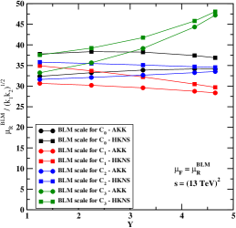
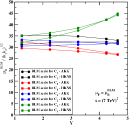
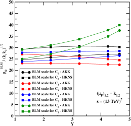
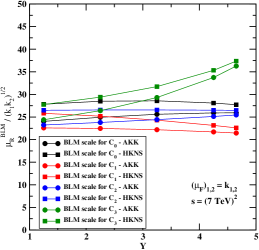
Figure 4.3: BLM scales for the dihadron production versus the rapidity interval $Y$ for the $\phi$-averaged cross section $C_{0}$ and for the azimuthal coefficients $C_{1,2,3}$. The two choices for the factorisation scale $\mu_{F}=\mu^{\rm BLM}_{R}$ and $(\mu_{F})_{1,2}=|\vec{k}_{1,2}|$ are considered, while the center-of-mass energy takes the values $\sqrt{s}=7,13$ TeV.

4.2 A first phenomenological analysis

In this Section the first stage of our analysis, with the implementation of a partial NLA BFKL in which we take only the higher-order corrections coming from the kernel and neglecting the NLA parts of hadron vertices, i.e. putting $\bar{c}^{(1)}_{1,2}=0$ in Eq. (4.13).

We found that the difference between our predictions for the $C_{m}/C_{n}$ ratios at $\sqrt{s}=13$ TeV (Fig. 4.4) and the ones at $\sqrt{s}=13$ TeV (Fig. 4.5), is not larger than $3\%$. We see on the first caption of Figs. 4.4 and 4.5. the sizeable difference between predictions of the $\phi$-averaged cross section $C_{0}$ in two cases of selected FFs, AKK and HKNS, which means that the FFs are not well constrained in the required kinematical region. In a similar range the difference between $\pi^{\pm}$ and $K^{\pm}$ AKK and HKNS FFs was recently discussed in Ref. [Yang:2015avi]. Our calculation with the AKK FFs gives bigger cross sections, whereas the difference between AKK and HKNS for the azimuthal ratios $C_{m}/C_{n}$ is small, since the FFs uncertainties are largely cancelled in the coefficient ratios describing the azimuthal-angle correlations. Our predictions for dihadron production calculated in LLA with the use of the “natural” scale $\mu_{N}$ and our NLA results obtained with the BLM scale setting are different: with NLA BLM we got much lower values of the cross sections and considerably larger predictions for the $C_{m}/C_{n}$. Plots of Figs. 4.4 and 4.5 show that the LLA results with BLM scales lie closer to the NLA BLM ones than LLA results with “natural” scales. The difference between NLA BLM and LLA with BLM scale predictions is due to the account of NLA corrections to the BFKL kernel in the former. This clearly represents a reliability test for the BLM method.

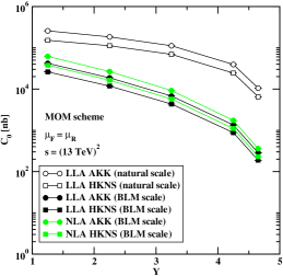
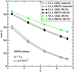
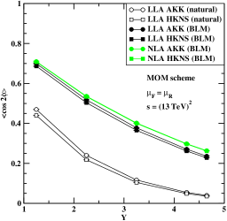
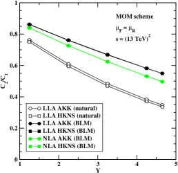
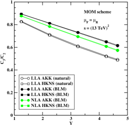
Figure 4.4: Cross section and azimuthal ratios for dihadron production for $\mu_{F}=\mu^{\rm BLM}_{R}$, $\sqrt{s}=13$ TeV, and $Y\leq 4.8$. Here “LLA” means pure leading logarithmic approximation, while “NLA kernel” means inclusion of the NLA corrections from the kernel only. See the text for the definition of “natural” and “BLM” scales.

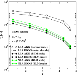
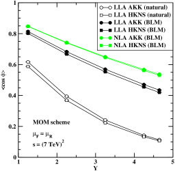
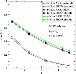
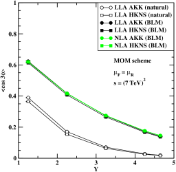
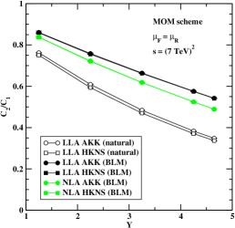
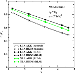
Figure 4.5: Cross section and azimuthal ratios for dihadron production for $\mu_{F}=\mu^{\rm BLM}_{R}$, $\sqrt{s}=7$ TeV, and $Y\leq 4.8$. Here “LLA” means pure leading logarithmic approximation, while “NLA kernel” means inclusion of the NLA corrections from the kernel only. See the text for the definition of “natural” and “BLM” scales.

4.3 Full NLA BFKL calculation

Int this section the first analysis for dihadron production in the full NLA BFKL accuracy is presented.

We checked that in our numerical analysis the essential values of $x$ are not too small, $x\sim[10^{-3}\div 10^{-2}]$, and even bigger in the case of the larger $Y\leq 9.4$. This justifies our use of PDFs with the standard DGLAP evolution. Note that our process is not a low-$x$ one, and similarly to the Mueller–Navelet jet production, we are dealing with a dilute partonic system. Therefore possible saturation effects are not important here, and the BFKL dynamics appears only through resummation effects in the hard scattering subprocesses, without influence on the PDF evolution.

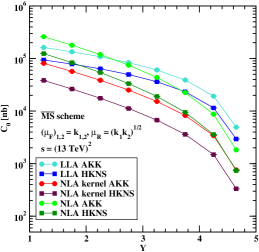
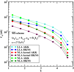
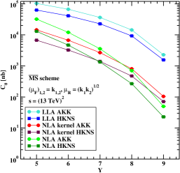
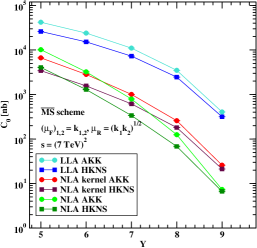
Figure 4.6: $Y$-dependence of $C_{0}$ in the $\overline{\rm MS}$ scheme (as implemented in Eq. (4.6)) at “natural” scales for $\mu_{R}$ and $\mu_{F}$, $\sqrt{s}=7,13$ TeV, and in the two cases of $Y\leq 4.8$ and $Y\leq 9.4$. Here and in the following figure captions “LLA” means pure leading logarithmic approximation, “NLA kernel” means inclusion of the NLA corrections from the kernel only, “NLA” stands for full inclusion of NLA corrections, i.e. both from the kernel and the hadron vertices.

In Fig. 4.6 we show our results for $C_{0}$ in the $\overline{\rm MS}$ scheme (as implemented in Eq. (4.6)) for we already specified above the scale settings $\sqrt{s}=7,13$ TeV, and in the two cases of $Y\leq 4.8$ and $Y\leq 9.4$. We clearly see that NLA corrections become negative with respect to the LLA prediction when $Y$ grows. Besides, it is interesting to note that the full NLA approach predicts larger values for the cross sections in comparison to the case where only NLA corrections to the BFKL kernel are taken into account. It means that the inclusion into the analysis of the NLA corrections to the hadron vertices makes the predictions for the cross sections somewhat bigger and partially compensates the large negative effect from the NLA corrections to the BFKL kernel.

The other results we presented below are obtained using BLM in the MOM scheme, as it is given in Eq. (4.13). In Figs. 4.7 and 4.8 we present our results for $C_{0}$ and for several ratios $C_{m}/C_{n}$ at $\sqrt{s}=13$ and $7$ TeV, respectively; $\mu_{F}$ is set equal to $\mu^{\rm BLM}_{R}$, while $Y\leq 4.8$. It is worth to note that in this case the NLA corrections to $C_{0}$ are positive, so they increase the value of the $\phi$-averaged cross section at all values of $Y$. This is the result of the combination of two distinct effects: on one side, we already saw in Ref. [Celiberto:2016hae] that changing the renormalisation scheme produces a non-exponentiated extra factor in Eq. (4.13) proportional to $T^{\rm conf}$, and that is positive. On the other side, we found that the $C_{gg}$ coefficient in Eq. (4.9) gives a large and positive contribution to the NLO impact factor. We see also that NLA corrections increase the azimuthal correlations: $C_{1}/C_{0}$, $C_{2}/C_{0}$, and $C_{3}/C_{0}$, while their effect is small with respect to LLA predictions in their ratios, $C_{2}/C_{1}$ and $C_{3}/C_{2}$. The value of $C_{1}/C_{0}$ for $Y\leq 2.75$ in some cases exceeds $1$. We consider this as an effect due to the fact that, at very small $Y$, which corresponds to the small values of partonic subenergies $\hat{s}$, we are crossing the applicability limit of the BFKL approach, which systematically neglects any contributions that are suppressed by the powers of $\hat{s}$.

For comparison, we show in Figs. 4.9 and 4.10 the results for the same observables with the choice of $(\mu_{F})_{1,2}=|\vec{k}_{1,2}|$. The patterns we have found are very similar to the previous ones, but we see that the effect of having $C_{1}/C_{0}$ larger than $1$ at small $Y$ is reduced. Furthermore, NLA corrections are negative for larger $Y$ values. On the basis of this, we may conclude that, in the $Y\leq 4.8$ kinematical regime, the choice of “natural” scales for $\mu_{F}$ stabilises the results.

In Figs. 4.11 and 4.12 we present our results for $C_{0}$ and for several ratios $C_{m}/C_{n}$ at $\sqrt{s}=13$ and $7$ TeV respectively; $\mu_{F}$ is set equal to $\mu^{\rm BLM}_{R}$, while $Y$ lies on a larger range, i.e. $Y\leq 9.4$.

For comparison, we show in Figs. 4.13 and 4.14 the results for the same observables with the choice of $(\mu_{F})_{1,2}=|\vec{k}_{1,2}|$. We clearly see that, in the case of larger rapidity intervals $Y$ and with the “natural” choice for the factorisation scale, the situation is different in comparison to the $\mu_{F}=\mu_{R}^{BLM}$ choice: the NLA corrections to the cross section $C_{0}$ are negative, while the pattern of $C_{1}/C_{0}$ shows a somewhat unexpected “turn-up” at large $Y$, and these effects are more pronounced for the lower LHC energy, $\sqrt{s}=7\ \rm{TeV}$. Such a sensitivity to the factorisation scale setting may be an indication of the fact that with the increase of $Y$ values we are moving towards the threshold region, where the energy of detected dihadron system becomes comparable with $\sqrt{s}$. In this situation the FFs and PDFs are probed in regions that are close to the end-points of their definitions, where they exhibit large dependence on the factorisation scale. From the physical site, in this kinematics the undetected hard-gluon radiation is getting restricted and only radiation of soft gluons is allowed. Soft-gluon radiation can not change the kinematics of the hard subprocess, therefore one expects restoration of the correlation of the detected hadrons in the relative azimuthal angle when we approach the threshold region. It is well known that in this situation large threshold double logarithms [Jager:2004jh, Kidonakis:1998bk, deFlorian:2007fv, Catani:1996yz] appear in the perturbative series, and such contributions have to be resummed to all orders. Threshold logarithms appear when the parent parton has just enough energy to produce the identified particle in the final state and the unobserved recoiling partonic final state. Resummation in the kinematics where both threshold and BFKL logarithms are important is an interesting task, but it goes well beyond the scope of the present study. Here we just note that pure BFKL predictions in the region of largest $Y$ become rather sensitive to the choice of the factorisation scale.

To better assess the factorization scale dependence, we have considered also the case when $\mu_{F}$ is varied around its “natural” value $\sqrt{|\vec{k}_{1}||\vec{k}_{2}|}$ by a factor $r$ taking values in the range 1/2 to four. In Fig. 4.15, as a selection of our results, we present the plots for $C_{0}$ and $C_{1}/C_{0}$ at a squared center-of-mass energy of 7 and 13 TeV for the rapidity region $Y\leq 4.8$ and the HKNS parametrization of the fragmentation functions.

It is worth to note that the general features of our predictions for dihadron production are rather similar to those obtained earlier for the Mueller–Navelet jet process. Although the BFKL resummation leads to the growth with energy of the partonic subprocess cross sections, the convolution of the latter with the proton PDFs makes the net effect of a decrease with $Y$ of our predictions. This is due to the fact that, at larger values of $Y$, PDFs are probed effectively at larger values of $x$, where they fall very fast. For the dihadron azimuthal correlations we predict a decreasing behaviour with $Y$. That originates from the increasing amount of hard undetected parton radiation in the final state allowed by the growth of the partonic subprocess energy.

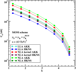
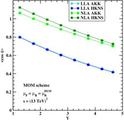
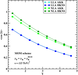
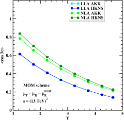
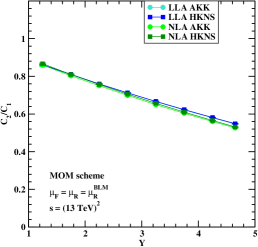
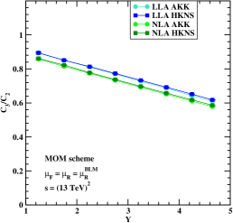
Figure 4.7: $Y$-dependence of $C_{0}$ and of several ratios $C_{m}/C_{n}$ for $\mu_{F}=\mu^{\rm BLM}_{R}$, $\sqrt{s}=13$ TeV, and $Y\leq 4.8$.

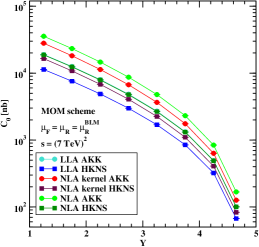
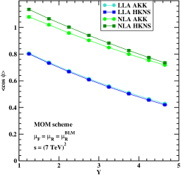
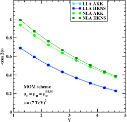
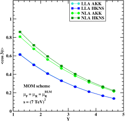
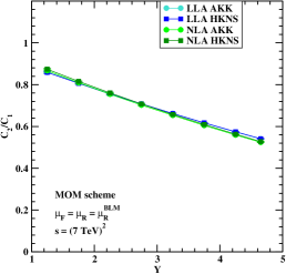
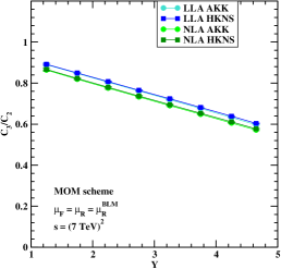
Figure 4.8: $Y$-dependence of $C_{0}$ and of several ratios $C_{m}/C_{n}$ for $\mu_{F}=\mu^{\rm BLM}_{R}$, $\sqrt{s}=7$ TeV, and $Y\leq 4.8$.

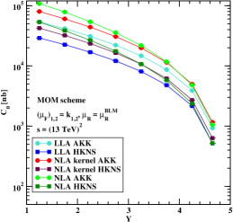
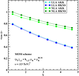
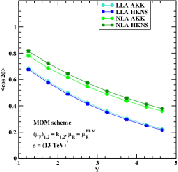
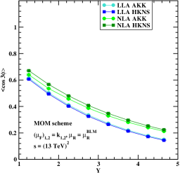
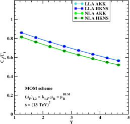
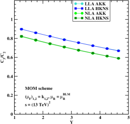
Figure 4.9: $Y$-dependence of $C_{0}$ and of several ratios $C_{m}/C_{n}$ for $(\mu_{F})_{1,2}=|\vec{k}_{1,2}|$, $\sqrt{s}=13$ TeV, and $Y\leq 4.8$.

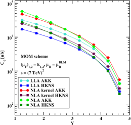
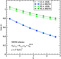
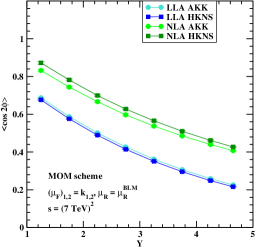
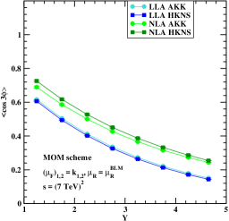
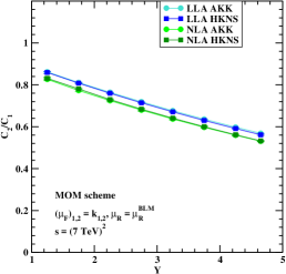
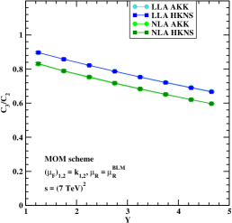
Figure 4.10: $Y$-dependence of $C_{0}$ and of several ratios $C_{m}/C_{n}$ for $(\mu_{F})_{1,2}=|\vec{k}_{1,2}|$, $\sqrt{s}=7$ TeV, and $Y\leq 4.8$.

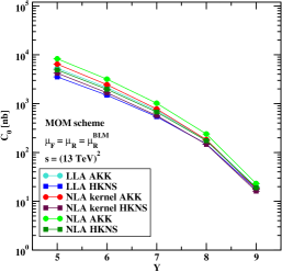
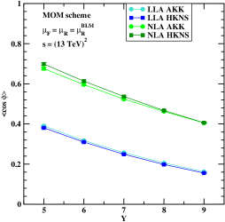
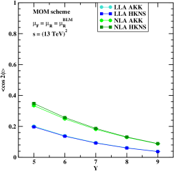
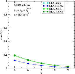
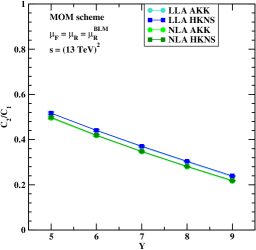
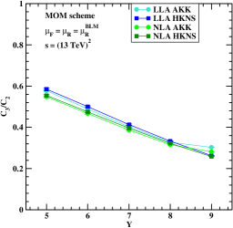
Figure 4.11: $Y$-dependence of $C_{0}$ and of several ratios $C_{m}/C_{n}$ for $\mu_{F}=\mu^{\rm BLM}_{R}$, $\sqrt{s}=13$ TeV, and $Y\leq 9.4$.

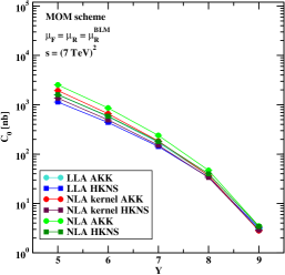
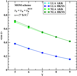
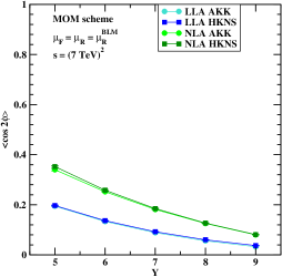
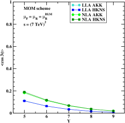
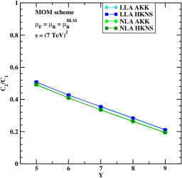
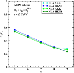
Figure 4.12: $Y$-dependence of $C_{0}$ and of several ratios $C_{m}/C_{n}$ for $\mu_{F}=\mu^{\rm BLM}_{R}$, $\sqrt{s}=7$ TeV, and $Y\leq 9.4$.

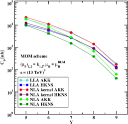
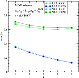
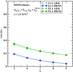
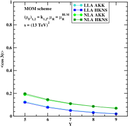
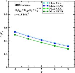
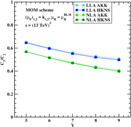
Figure 4.13: $Y$-dependence of $C_{0}$ and of several ratios $C_{m}/C_{n}$ for $(\mu_{F})_{1,2}=|\vec{k}_{1,2}|$, $\sqrt{s}=13$ TeV, and $Y\leq 9.4$.

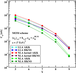
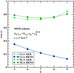
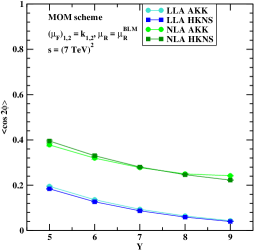
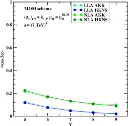
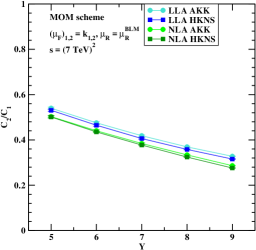
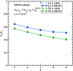
Figure 4.14: $Y$-dependence of $C_{0}$ and of several ratios $C_{m}/C_{n}$ for $(\mu_{F})_{1,2}=|\vec{k}_{1,2}|$, $\sqrt{s}=7$ TeV, and $Y\leq 9.4$.

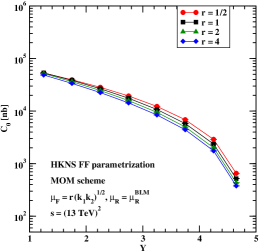
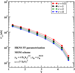
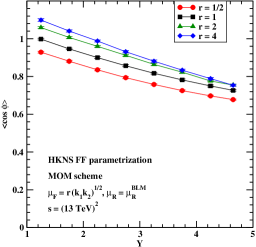
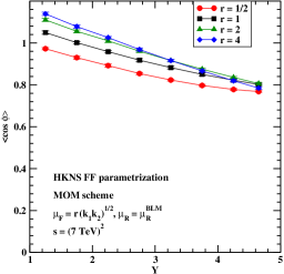
Figure 4.15: $Y$-dependence of $C_{0}$ and of $C_{1}/C_{0}$ for $\mu_{F}=r\sqrt{|\vec{k}_{1}||\vec{k}_{2}|}$, with $r=1/2,1,2,4$, and $Y\leq 4.8$.

4.4 Numerical specifics

4.4.1 Used tools

All the numerical calculations presented in Section 4.2 and in Section 4.3 were performed in Fortran, choosing a two-loop running coupling setup with $\alpha_{s}\left(M_{Z}\right)=0.11707$ and five quark flavours. It is known that potential sources of uncertainty could be due to the particular PDF and FF parameterisations used. For this reason, preliminary tests were done by using three different NLO PDF sets, expressly: MSTW 2008 [Martin:2009iq], MMHT 2014 [Harland-Lang:2014zoa], and CT 2014 [Dulat:2015mca], and convolving them with the three following NLO FF routines: AKK [Albino:2008fy], DSS [deFlorian:2007aj, deFlorian:2007ekg], and HNKS [Hirai:2007cx]. Our tests have shown no significant discrepancy when different PDF sets are used in our kinematical range. In view of this result, in the final calculations the MSTW 2008 PDF set (which was successfully used in various analyses of inclusive semi-hard processes at the LHC, including our previous studies of Mueller–Navelet jets) was selected, together with the FF interfaces mentioned above. The results with the DSS routine are not shown, since they would be hardly distinguishable from those with the HKNS parameterisation.

Specific CERN program libraries [cernlib] were used to evaluate the azimuthal coefficients given in Eq. (4.13), which requires a complicated 8-dimensional numerical integration (the expressions for $\bar{c}^{(1)}_{1,2}$ contain an additional longitudinal fraction integral in comparison to the formulæ for the LLA vertices, given in Eqs. (4.7) and (4.8)). Furthermore, slightly modified versions of the Chyp [chyp] and Psi [RpsiCody:1973] routines were used to calculate the Gauss hypergeometric function ${}_{2}F_{1}$ and the real part of the $\psi$ function, respectively.

4.4.2 Uncertainty estimation

The most significant uncertainty comes from the numerical 4-dimensional integration over the two transverse momenta $|\vec{k}_{1,2}|$, the rapidity $y_{1}$, and over $\nu$. Its effect was directly estimated by Dadmul integration routine [cernlib]. The other three sources of uncertainty, which are respectively: the one-dimensional integration over the parton fraction $x$ needed to perform the convolution between PDFs and FFs in the LO/NLO impact factors (see Eq. (4.7) and (4.9)), the one-dimensional integration over the longitudinal momentum fraction $\zeta$ in the NLO impact factor correction (see Eqs. (4.9)), and the upper cutoff in the numerical integrations over $|\vec{k}_{1,2}|$ and $\nu$, are negligible with respect to the first one. For this reason the error bars of all predictions presented in this work are just those given by the Dadmul routine.

4.5 Summary

We studied the inclusive dihadron production process at the LHC within the BFKL approach, giving the first complete phenomenological predictions for cross sections and azimuthal correlation momenta in the full NLA approximation. We implemented the exact version of the BLM optimisation procedure, which requires the choice of renormalisation scale $\mu_{R}=\mu_{R}^{BLM}$ such that it makes completely vanish the NLA terms proportional to the QCD $\beta$-function. This procedure leads to rather large values of the scale $\mu_{R}^{BLM}$ and it allows to minimise the size of the NLA corrections in our observables. We considered two center-of-mass energies, $\sqrt{s}=7,13$ TeV, and two different ranges for the rapidity interval between the two hadrons in the final state, $Y\leq 4.8$ and $Y\leq 9.4$, which are typical for the last CMS analyses. The first rapidity range we investigated, $Y\leq 4.8$, may look to be not large enough for the dominance of BFKL dynamics. But we see, however, that in this range there are large NLA BFKL corrections, thus indicating that the BFKL resummation is playing here a non-trivial role. To clarify the issue it would be very interesting to confront our predictions with the results of fixed-order NLO DGLAP calculations. But this would require new numerical analysis in our semi-hard kinematical range, because the existing NLO DGLAP results cover the hard kinematical range for the energies of fixed target experiments, see for instance Refs. [Owens:2001rr, Almeida:2009jt].

As for the hadron’s transverse momenta, we imposed the symmetric lower cutoff: $|\vec{k}_{1,2}|\geq 5$ GeV. Considering a region of lower hadron transverse momenta, say $|\vec{k}_{1,2}|\geq 2$ GeV, would lead to even larger values of the cross sections. But it should be noted that in our calculation we use the BFKL method together with leading-twist collinear factorisation, which means that we are systematically neglecting power-suppressed corrections. Therefore, going to smaller transverse momenta we would enter a region where higher-twist effects must be important.

The general features of our predictions for dihadron production are rather similar to those obtained earlier for the Mueller-Navelet jet process. In particular, we observe that the account of NLA BFKL terms leads to much less azimuthal angle decorrelation with increasing $Y$ in comparison to LLA BFKL calculations. As for the difference between the Mueller-Navelet jet and dihadron production processes, we would mention the fact that, contrary to the jets’ case, the full account of NLA terms leads in dihadron production to an increase of our predictions for the cross sections in comparison to the LLA BFKL calculation.

We considered the effect of using different parameterisation sets for the PDFs and the FFs, that could potentially give rise to uncertainties which, in principle, are not negligible. We did some preliminary tests devoted to gauge the effect of using different PDF routines, showing that it leads to no significant difference in the results. Then, we investigated the $Y$-behaviour of our observables by using two different FF parameterisations. Our calculation with the AKK FFs gives bigger cross sections, while the difference between AKK and HKNS is small, since the FFs uncertainties are mostly wiped out in the azimuthal ratios.

We studied the effect of using two different choices for the factorisation scale, $\mu_{F}=\mu_{R}^{\rm BLM}$ and $(\mu_{F})_{1,2}=|\vec{k}_{1,2}|$, whereas $\mu_{R}=\mu_{R}^{\rm BLM}$ runs at BLM scales. We see some difference in predictions within these two approaches, especially for larger values of $Y$ and at the smaller value of the energy $\sqrt{s}=7\ \rm{TeV}$. In this region, the kinematical restriction for the undetected hard gluon radiation may start to be important, requiring resummation of threshold double logarithms together with BFKL logarithms of energy. In this case, the phase space available for gluon bremsstrahlung vanishes, so that only soft and collinear emission is allowed, resulting in large logarithmic corrections to the partonic cross section. This issue maybe a physical reason for the observed strong dependence on the factorisation scale choice in our pure BFKL approach, and it definitely deserves a further study.

Appendix C

NLO impact factor for the identified hadron

In this Appendix the expressions for the NLO coefficient functions $C_{ij}$ in Eq. (4.9) are given (see Ref. [hadrons] for further details). In particular, we have:

$$C_{gg}\left(x,\zeta\right)=P_{gg}(\zeta)\left(1+\zeta^{-2\gamma}\right)\ln\left(\frac{\vec{k}_{h}^{2}x^{2}\zeta^{2}}{\mu_{F}^{2}\alpha_{h}^{2}}\right)-\frac{\beta_{0}}{2}\ln\left(\frac{\vec{k}_{h}^{2}x^{2}\zeta^{2}}{\mu^{2}_{R}\alpha_{h}^{2}}\right)$$ (C.1)

$$+\,\delta(1-\zeta)\left[C_{A}\ln\left(\frac{s_{0}\,\alpha_{h}^{2}}{\vec{k}^{2}_{h}\,x^{2}}\right)\chi(n,\gamma)-C_{A}\left(\frac{67}{18}-\frac{\pi^{2}}{2}\right)+\frac{5}{9}n_{f}\right.$$

$$\left.+\frac{C_{A}}{2}\left(\psi^{\prime}\left(1+\gamma+\frac{n}{2}\right)-\psi^{\prime}\left(\frac{n}{2}-\gamma\right)-\chi^{2}(n,\gamma)\right)\right]$$

$$+\,C_{A}\left(\frac{1}{\zeta}+\frac{1}{(1-\zeta)_{+}}-2+\zeta\bar{\zeta}\right)$$

$$\times\,\left(\chi(n,\gamma)(1+\zeta^{-2\gamma})-2(1+2\zeta^{-2\gamma})\ln\zeta+\frac{\bar{\zeta}^{2}}{\zeta^{2}}I_{2}\right)$$

$$+\,2\,C_{A}(1+\zeta^{-2\gamma})\left(\left(\frac{1}{\zeta}-2+\zeta\bar{\zeta}\right)\ln\bar{\zeta}+\left(\frac{\ln(1-\zeta)}{1-\zeta}\right)_{+}\right)\ ,$$

$$C_{gq}\left(x,\zeta\right)=P_{qg}(\zeta)\left(\frac{C_{F}}{C_{A}}+\zeta^{-2\gamma}\right)\ln\left(\frac{\vec{k}_{h}^{2}x^{2}\zeta^{2}}{\mu_{F}^{2}\alpha_{h}^{2}}\right)$$ (C.2)

$$+\,2\,\zeta\bar{\zeta}\,T_{R}\,\left(\frac{C_{F}}{C_{A}}+\zeta^{-2\gamma}\right)+\,P_{qg}(\zeta)\,\left(\frac{C_{F}}{C_{A}}\,\chi(n,\gamma)+2\zeta^{-2\gamma}\,\ln\frac{\bar{\zeta}}{\zeta}+\frac{\bar{\zeta}}{\zeta}I_{3}\right)\ ,$$

$$C_{qg}\left(x,\zeta\right)=P_{gq}(\zeta)\left(\frac{C_{A}}{C_{F}}+\zeta^{-2\gamma}\right)\ln\left(\frac{\vec{k}_{h}^{2}x^{2}\zeta^{2}}{\mu_{F}^{2}\alpha_{h}^{2}}\right)$$ (C.3)

$$+\zeta\left(C_{F}\zeta^{-2\gamma}+C_{A}\right)+\,\frac{1+\bar{\zeta}^{2}}{\zeta}\left[C_{F}\zeta^{-2\gamma}(\chi(n,\gamma)-2\ln\zeta)+2C_{A}\ln\frac{\bar{\zeta}}{\zeta}+\frac{\bar{\zeta}}{\zeta}I_{1}\right]\ ,$$

$$C_{qq}\left(x,\zeta\right)=P_{qq}(\zeta)\left(1+\zeta^{-2\gamma}\right)\ln\left(\frac{\vec{k}_{h}^{2}x^{2}\zeta^{2}}{\mu_{F}^{2}\alpha_{h}^{2}}\right)-\frac{\beta_{0}}{2}\ln\left(\frac{\vec{k}_{h}^{2}x^{2}\zeta^{2}}{\mu^{2}_{R}\alpha_{h}^{2}}\right)$$ (C.4)

$$+\,\delta(1-\zeta)\left[C_{A}\ln\left(\frac{s_{0}\,\alpha_{h}^{2}}{\vec{k}^{2}_{h}\,x^{2}}\right)\chi(n,\gamma)+C_{A}\left(\frac{85}{18}+\frac{\pi^{2}}{2}\right)-\frac{5}{9}n_{f}-8\,C_{F}\right.$$

$$\left.+\frac{C_{A}}{2}\left(\psi^{\prime}\left(1+\gamma+\frac{n}{2}\right)-\psi^{\prime}\left(\frac{n}{2}-\gamma\right)-\chi^{2}(n,\gamma)\right)\right]+\,C_{F}\,\bar{\zeta}\,(1+\zeta^{-2\gamma})$$

$$+\left(1+\zeta^{2}\right)\left[C_{A}(1+\zeta^{-2\gamma})\frac{\chi(n,\gamma)}{2(1-\zeta)_{+}}+\left(C_{A}-2\,C_{F}(1+\zeta^{-2\gamma})\right)\frac{\ln\zeta}{1-\zeta}\right]$$

$$+\,\left(C_{F}-\frac{C_{A}}{2}\right)\left(1+\zeta^{2}\right)\left[2(1+\zeta^{-2\gamma})\left(\frac{\ln(1-\zeta)}{1-\zeta}\right)_{+}+\frac{\bar{\zeta}}{\zeta^{2}}I_{2}\right]\;,$$

with the plus-prescription defined in Eq. (B.6).

Here $\gamma=i\nu-1/2$, while $P_{ij}(\zeta)$ are leading order DGLAP kernels defined in Appendix B. The expressions for the $I_{1,2,3}$ functions are given in Appendix B.

Chapter 5 Three-jet production

In the last two Chapters we investigated semi-hard processes with two objects (jets or charged light hadrons) always tagged in the final state. We started from the expression of the forward parton impact factors [Fadin:1999de, Fadin:1999df], ‘opening’ one of the integrations over the intermediate-state phase space to allow one parton to generate the detected object in the final state. Thus, we obtained the expressions for the process-dependent vertex, which have to be convoluted (Eq. (2.70)) with the universal Green’s function in order to get the cross section for the considered processes.

Inclusive multi-jet production represents a further step towards the study of BFKL dynamics in a much more exclusive way. While in the two-body case we modified the expression of the parton impact factors in order to allow the detection of two objects in the fragmentation region of the respective parent proton, in the $n$-body case we need to suitably generalise our formalism to account for the emission of extra particles in more central regions covered by the LHC detectors. The first advance in this direction, presented in this Chapter, is to propose new observables associated to the inclusive production of three jets: two of them are the original Mueller–Navelet jets, while the third one is tagged in central regions of rapidity.

When a jet central in rapidity is emitted in the final state, it is possible to single out an extra gluon emission by extracting its emission probability from the BFKL kernel. For further details and a more specific discussion, we refer to Refs. [Bartels:2006hg, Schwennsen:2007hs] and to the preliminary discussion given in Section 5.2.5, respectively. The three-jet cross section can be constructed in this way:

$$\sigma^{\rm 3-jet}(s)=\frac{1}{(2\pi)^{2}}\int\frac{d^{2}\vec{q}_{1}}{\vec{q}_{1}^{\,\,2}}\int\frac{d^{2}\vec{q}_{2}}{\vec{q}_{2}^{\,\,2}}\Phi_{1}(\vec{q}_{1},s_{0})\Phi_{2}(-\vec{q}_{2},s_{0})$$ (5.1)

$$\times\,\int d^{2}\vec{q_{A}}\int d^{2}\vec{q_{B}}\int\limits^{\delta+i\infty}_{\delta-i\infty}\frac{d\omega}{2\pi i}\left(\frac{s}{s_{0}}\right)^{\omega}G_{\omega}(\vec{q}_{1},\vec{q}_{A})$$

$$\times\,\Phi_{C}(-\vec{q}_{A},\vec{q}_{B},s_{0})\int\limits^{\delta+i\infty}_{\delta-i\infty}\frac{d\omega^{\prime}}{2\pi i}\left(\frac{s}{s_{0}}\right)^{\omega^{\prime}}G_{\omega}^{\prime}(\vec{q}_{B},\vec{q}_{2})\;,$$

where $\Phi_{1,2}$ are the two impact factors which describe the two forward/backward jets (as in the Mueller–Navelet case), while $\Phi_{C}$ is the central-jet emission vertex [Bartels:2006hg]. By selecting one emission to be exclusive we have factorised the Green’s function into two components. Each of them connects one of the external jets to the central one.

We will give predictions for the new azimuthal correlation momenta defined as

$${\cal R}^{MN}_{PQ}=\frac{\langle\cos{(M\,\Delta\phi_{\widehat{AJ}})}\cos{(N\,\Delta\phi_{\widehat{JB}})}\rangle}{\langle\cos{(P\,\Delta\phi_{\widehat{AJ}})}\cos{(Q\,\Delta\phi_{\widehat{JB}})}\rangle}\,,$$ (5.2)

where $\Delta\phi_{\widehat{AJ}}$ and $\Delta\phi_{\widehat{JB}}$ are, respectively, the azimuthal-angle difference between the first and the second (central) jet and between this one and the third jet (see Fig. 5.1). The distribution ratios defined in Eq. (5.2) generalise the $R_{MN}$ ratios typical of two-body final-state processes, as the previously discussed Mueller–Navelet jet (see Chapter 3) and dihadron (see Chapter 4) production processes, by showing an extra dependence on transverse momentum and rapidity of the central jet. Cross sections are calculated using collinear factorisation to produce the two most forward/backward jets, taking the convolution of the partonic cross section, which follows the BFKL dynamics, with collinear PDFs included in the forward jet vertex. These two Mueller–Navelet jet vertices are linked to the centrally produced jet via two BFKL Green’s functions. To simplify our predictions, we integrate over the momenta of all produced jets, using current LHC experimental cuts.

This Chapter is organised as follows: In Section 5.1 the main formulæ are given, including a first analysis at partonic level; in Section 5.2 hadronic level predictions are presented, with the inclusion of NLA BFKL corrections together with BLM scales and for three different kinematical configurations (see Sections 5.2.3, 5.2.4 and 5.2.5). The section Summary is given in LABEL:sec:4j-summary.

The analysis given in this Chapter is based on the work done in Refs. [Caporale:2015vya, Caporale:2016soq, Caporale:2016zkc] and presented in Refs. [Celiberto:2016vhn, Caporale:2016oxl, Chachamis:2016lyi, Caporale:2016pqe, Caporale:2016djm, Caporale:2016lnh, Chachamis:2017:dis].

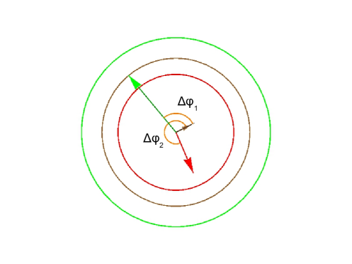
Figure 5.1: Representation of a three-jet event in a generic detector. All three circles are perpendicular to the beam axis.

5.1 A new way to probe BFKL

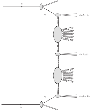
Figure 5.2: Inclusive three-jet production process in multi-Regge kinematics.

5.1.1 The three-jet cross section

The process under investigation (see Figs. 5.1 and 5.2) is the production of two forward/backward jets, both characterised by high transverse momenta $\vec{k}_{A,B}$ and well separated in rapidity, together with a third jet produced in the central rapidity region and with possible associated minijet production. This corresponds to

$${\rm p}(p_{1})\,+\,{\rm p}(p_{2})\,\to\,{\rm j}_{A}(k_{A})\,+\,{\rm j}_{C}(k_{J})\,+\,{\rm j}_{B}(k_{B})\,+\,{\rm minijets}\;,$$ (5.3)

where ${\rm j}_{A}$ is the forward jet with transverse momentum $\vec{k}_{A}$ and rapidity $Y_{A}$, ${\rm j}_{B}$ is the backward jet with transverse momentum $\vec{k}_{B}$ and rapidity $Y_{B}$ and ${\rm j}_{C}$ is the central jet with transverse momentum $\vec{k}_{J}$ and rapidity $y_{J}$.

In collinear factorisation the cross section for the process (5.3) reads

$$\frac{d\sigma^{3-{\rm jet}}}{dk_{A}\,dY_{A}\,d\theta_{A}\,dk_{B}\,dY_{B}\,d\theta_{B}\,dk_{J}\,dy_{J}d\theta_{J}}$$ (5.4)

$$=\sum_{r,s=q,{\bar{q}},g}\int_{0}^{1}dx_{1}\int_{0}^{1}dx_{2}\ f_{r}\left(x_{1},\mu_{F}\right)\ f_{s}\left(x_{2},\mu_{F}\right)\;d{\hat{\sigma}^{3-{\rm jet}}}_{r,s}\left(\hat{s},\mu_{F}\right)\;,$$

where the $r,s$ indices specify the parton types (quarks $q=u,d,s,c,b$; antiquarks $\bar{q}=\bar{u},\bar{d},\bar{s},\bar{c},\bar{b}$; or gluon $g$), $f_{r,s}\left(x,\mu_{F}\right)$ are the initial proton PDFs; $x_{1,2}$ represent the longitudinal fractions of the partons involved in the hard subprocess; $d{\hat{\sigma}^{3-{\rm jet}}}_{r,s}\left(\hat{s},\mu_{F}\right)$ is the partonic cross section for the production of jets and $x_{1}x_{2}s\equiv\hat{s}$ is the squared center-of-mass energy of the hard subprocess (see Fig. 5.2). The BFKL dynamics enters in the cross section for the partonic hard subprocess $d{\hat{\sigma}^{3-{\rm jet}}}_{r,s}$ (in the form of two forward Green’s functions $\varphi$ to be described in a while), which can be presented as (from here we start to use the notation $k_{A,B,Y}\equiv|\vec{k}_{A,B,Y}|$, which holds in the following):

$$\frac{d{\hat{\sigma}^{3-{\rm jet}}}_{r,s}}{dk_{J}d\theta_{J}dy_{J}}=\frac{\bar{\alpha}_{s}}{\pi k_{J}}\int d^{2}\vec{p}_{A}\int d^{2}\vec{p}_{B}\,\delta^{(2)}\left(\vec{p}_{A}+\vec{k}_{J}-\vec{p}_{B}\right)$$ (5.5)

$$\times\,\varphi\left(\vec{k}_{A},\vec{p}_{A},Y_{A}-y_{J}\right)\varphi\left(\vec{p}_{B},\vec{k}_{B},y_{J}-Y_{B}\right)\;,$$

where $\bar{\alpha}_{s}=N_{c}/\pi\,\alpha_{s}$, with $N_{c}$ the number of colours in QCD. In order to lie within MRK, we have considered the ordering in the rapidity of the produced particles $Y_{A}>y_{J}>Y_{B}$, while $k_{J}^{2}$ is always above the experimental resolution scale. $\varphi\left(\vec{p},\vec{q},0\right)$ is a suitable redefinition of the BFKL Green’s function, which now encode also the momentum two-dimensional delta coming from the LO jet function (Eq. (3.2)). In this way, some pieces of the LO jet vertex (Eq. (3.3)) are encoded in a very useful expression for the Green function, which holds at LLA.

It is possible algebraically manipulate the expression given in Eq. (5.5) in order to find distinct BFKL features. First of all, one can integrate the two-dimensional delta function in Eq. (5.5), to obtain

$$\frac{d{\hat{\sigma}^{3-{\rm jet}}}_{r,s}}{d^{2}\vec{k}_{J}dy_{J}}=\frac{\bar{\alpha}_{s}}{\pi k_{J}^{2}}\int dp^{2}d\theta\;\varphi(\vec{k}_{A},\vec{p},Y_{A}-y_{J})\varphi(\vec{p}+\vec{k}_{J},\vec{k}_{B},y_{J}-Y_{B})\;.$$ (5.6)

Then, the Green’s function can be expanded in Fourier components of the azimuthal angle to write:

$$\frac{d{\hat{\sigma}^{3-{\rm jet}}}_{r,s}}{d^{2}\vec{k}_{J}dy_{J}}=\frac{\bar{\alpha}_{s}}{\pi k_{J}^{2}}\sum_{m,n=-\infty}^{+\infty}e^{i(m\theta_{A}-n\theta_{B})}\>\>\Omega_{m,n}\left(\vec{k_{A}},\vec{k_{B}},Y_{A},Y_{B},\vec{k_{J}},\theta_{J},y_{J}\right)\;,$$ (5.7)

where

$$\Omega_{m,n}\left(\vec{k_{A}},\vec{k_{B}},Y_{A},Y_{B},\vec{k_{J}},\theta_{J},y_{J}\right)$$ (5.8)

$$=\int_{0}^{+\infty}dp\,p\int_{0}^{2\pi}d\theta e^{i\left[n\arctan\left(\frac{p\sin\theta+k_{J}\sin\theta_{J}}{p\cos\theta+k_{J}\cos\theta_{J}}\right)-m\theta\right]}\varphi_{m}\left(|\vec{k_{A}}|,|\vec{p_{A}}|,Y_{A}-y_{J}\right)$$

$$\times\,\varphi_{n}\left(\sqrt{p^{2}+k_{J}^{2}+2|\vec{p}||\vec{k}_{J}|\cos\left(\theta-\theta_{J}\right)},|\vec{p_{B}}|,y_{J}-Y_{B}\right)\;.$$

Here $\varphi_{i}$ is the $i$-th azimuthal component of the Green’s function obtained after the projection on the $(\nu,n)$-space, whose LLA and NLA expressions are given respectively in Eqs. (5.15) and (5.27). Using the relation $\arctan\alpha=\frac{i}{2}\ \ln\left(\frac{1-i\alpha}{1+i\alpha}\right)$, which holds for any real $\alpha$, one has

$$\Omega_{m,n}\left(\vec{k_{A}},\vec{k_{B}},Y_{A},Y_{B},\vec{k_{J}},\theta_{J},y_{J}\right)$$ (5.9)

$$=\int_{0}^{+\infty}dp\,p\int_{0}^{2\pi}d\theta\>e^{-im\theta}\,\left(\frac{pe^{i\theta}+k_{J}e^{i\theta_{J}}}{pe^{-i\theta}+k_{J}e^{-i\theta_{J}}}\right)^{\frac{n}{2}}$$

$$\times\,\varphi_{m}\left(|\vec{k_{A}}|,|\vec{p_{A}}|,Y_{A}-y_{J}\right)$$

$$\times\,\varphi_{n}\left(\sqrt{p^{2}+k_{J}^{2}+2|\vec{p}||\vec{k}_{J}|\cos\left(\theta-\theta_{J}\right)},|\vec{p_{B}}|,y_{J}-Y_{B}\right)\;.$$

The dependence on $\theta_{J}$ can be factorised out by making the change of variable $\theta-\theta_{J}\to\theta$. The final expression for $\Omega_{m,n}$ reads:

$$\Omega_{m,n}\left(\vec{k_{A}},\vec{k_{B}},Y_{A},Y_{B},\vec{k_{J}},\theta_{J},y_{J}\right)=$$ (5.10)

$$\>e^{i(n-m)\theta_{J}}\,\int_{0}^{+\infty}dp\,p\int_{0}^{2\pi}d\theta\>\frac{e^{-im\theta}\,\left(pe^{i\theta}+k_{J}\right)^{n}}{\sqrt{\left(p^{2}+k_{J}^{2}+2|\vec{p}||\vec{k}_{J}|\cos\theta\right)^{n}}}$$

$$\varphi_{m}\left(|\vec{k_{A}}|,|\vec{p_{A}}|,Y_{A}-y_{J}\right)\varphi_{n}\left(\sqrt{p^{2}+k_{J}^{2}+2|\vec{p}||\vec{k}_{J}|\cos\theta},|\vec{p_{B}}|,y_{J}-Y_{B}\right)\;.$$

In Sections 5.1.2 and 5.1.3 we investigate the properties of two new, generalised and suitable BFKL observables that the developed formalism allows us to define.

5.1.2 One-cosine projection: À la Mueller–Navelet

5.1.2.1 One-cosine azimuthal correlations

The first step is to integrate over the azimuthal angle of the central jet and over the difference in azimuthal angle between the two forward jets, $\Delta\phi=\theta_{A}-\theta_{B}-\pi$, to define a quantity similar to the usual Mueller–Navelet case, i.e.,

$$\int_{0}^{2\pi}d\Delta\phi\,\cos{\left(M\Delta\phi\right)}\int_{0}^{2\pi}d\theta_{J}\,\frac{d{\hat{\sigma}^{3-{\rm jet}}}_{r,s}}{dk_{J}d\theta_{J}dy_{J}}$$ (5.11)

$$=\frac{\bar{\alpha}_{s}}{2\pi}\sum_{L=0}^{M}\int_{0}^{\infty}dp^{2}\int_{0}^{2\pi}d\theta\frac{(-1)^{M}\left(\begin{array}[]{c}M\\ L\end{array}\right)\left(k_{J}^{2}\right)^{\frac{L-1}{2}}\,\left(p^{2}\right)^{\frac{M-L}{2}}\cos{\left(L\,\theta\right)}}{\sqrt{\left(p^{2}+k_{J}^{2}+2|\vec{p}||\vec{k}_{J}|\cos{\theta}\right)^{M}}}$$ (5.14)

$$\times\,\varphi^{\rm(LLA)}_{M}\left(|\vec{k_{A}}|,|\vec{p}|,Y_{A}-y_{J}\right)$$

$$\times\,\varphi^{\rm(LLA)}_{M}\left(\sqrt{p^{2}+k_{J}^{2}+2|\vec{p}||\vec{k}_{J}|}\cos{\theta},|\vec{k_{B}}|,y_{J}-Y_{B}\right)\;,$$

where $\varphi^{\rm(LLA)}_{n}$ is the Green’s function at LLA

$$\varphi^{\rm(LLA)}_{n}\left(|\vec{k}|,|\vec{q}|,y\right)\; =\;2\,\int_{0}^{\infty}d\nu\cos{\left(\nu\ln{\frac{k^{2}}{q^{2}}}\right)}\frac{e^{\bar{\alpha}_{s}\chi(n,\nu)y}}{\pi\sqrt{k^{2}q^{2}}}\;.$$ (5.15)

It is worth to note that, since the LO jet vertex (Eq. (3.8)) does not depend on $\nu$, we can let the Green’s function encode the $\nu$-integration. This second, suitable redefinition of the Green’s function is no more valid when NLO jet vertices (Eq. (B.1)) are considered. One of the experimental observables we want to highlight here corresponds to the mean value of the cosine of $\Delta\phi$ in the recorded events:

$$\langle\cos{\left(M\left(\Delta\phi\right)\right)}\rangle_{d{\hat{\sigma}^{3-{\rm jet}}}_{r,s}}=\frac{\int_{0}^{2\pi}d\Delta\phi\,\cos{\left(M\Delta\phi\right)}\int_{0}^{2\pi}d\theta_{J}\,\frac{d{\hat{\sigma}^{3-{\rm jet}}}_{r,s}}{d^{2}\vec{k}_{J}dy_{J}}}{\int_{0}^{2\pi}d\Delta\phi\int_{0}^{2\pi}d\theta_{J}\,\frac{d{\hat{\sigma}^{3-{\rm jet}}}_{r,s}}{d^{2}\vec{k}_{J}dy_{J}}}\;.$$ (5.16)

The perturbative stability (including renormalisation scale dependence) of the mean value defined above can be significantly improved (see Ref. [Caporale:2013uva] for a related discussion) if the contribution coming from the zero conformal spin, which corresponds to the index $n=0$ in Eq. (5.15), is removed. This can be achieved by defining the ratios

$${\cal R}_{N}^{M}=\frac{\langle\cos{\left(M\left(\Delta\phi\right)\right)}\rangle_{d{\hat{\sigma}^{3-{\rm jet}}}_{r,s}}}{\langle\cos{\left(N\left(\Delta\phi\right)\right)}\rangle_{d{\hat{\sigma}^{3-{\rm jet}}}_{r,s}}}\;,$$ (5.17)

where we consider $M,N$ as positive integers.

5.1.2.2 Numerical analysis

The observables defined in Eq. (5.17) allow us to perform different kinds of analysis at the partonic level. A first study, where the transverse momenta of the forward jets are fixed to $k_{A}=35$ GeV and $k_{B}=38$ GeV, done in Ref. [Caporale:2015vya], is presented in this Section.

Figure 5.3: A study of the ratio ${\cal R}_{1}^{2}$ as defined in Eq. (5.17) for fixed values of the $p_{t}$ of the two forward jets and two values of the $p_{t}$ of the tagged central jet, as a function of the rapidity difference between the two forward jets for the rapidity of the central jet chosen as $y_{J}=(Y_{A}-Y_{B})/2$.

The rapidity of the central jet is also fixed to be one half of the rapidity difference between the two forward jets: $y_{J}=(Y_{A}-Y_{B})/2$ simply because this allows us to connect with the well-known Mueller–Navelet jets. In this way one can study, e.g., the behaviour of the ratio ${\cal R}_{1}^{2}$ in Fig. 5.3 for two values of the transverse momentum of the central jet $k_{J}=35,40$ GeV. We see that this ratio decreases as a function of $Y_{A}-Y_{B}$. This is a consequence of the increase of the available phase space for inclusive minijet radiation and that the $n=1$ component decreases which energy slower that the $n=2$ one.

In the BFKL formalism one has that the larger the $n$ the slower the evolution with rapidity differences. This is very important since it is distinct from other approaches where QCD coherence is introduced as it was shown in Ref. [Chachamis:2011rw].

5.1.3 Two-cosine projection: generalised azimuthal correlations

5.1.3.1 Two-cosine azimuthal correlations

In this Section new observables, whose associated distributions have a very different behaviour to the ones characteristic of the Mueller–Navelet case, are proposed. These new distributions are defined using the projections on the two relative azimuthal angles formed by each of the forward jets with the central jet,

$$\Delta\phi_{\widehat{AJ}} =\theta_{A}-\theta_{J}-\pi$$ (5.18)

$$\Delta\phi_{\widehat{JB}} =\theta_{J}-\theta_{B}-\pi\;,$$

in the form

$$\int_{0}^{2\pi}d\theta_{A}\int_{0}^{2\pi}d\theta_{B}\int_{0}^{2\pi}d\theta_{J}\cos{\left(M\Delta\phi_{\widehat{AJ}}\right)}\cos{\left(N\Delta\phi_{\widehat{JB}}\right)}\frac{d^{3}\sigma^{3-{\rm jet}}}{dk_{J}d\theta_{J}dy_{J}}$$ (5.19)

$$=\bar{\alpha}_{s}\sum_{L=0}^{N}\left(\begin{array}[]{c}N\\ L\end{array}\right)\left(k_{J}^{2}\right)^{\frac{L-1}{2}}\int_{0}^{\infty}dp^{2}\,\left(p^{2}\right)^{\frac{N-L}{2}}$$

$$\times\,\int_{0}^{2\pi}d\theta\frac{(-1)^{M+N}\cos{\left(M\theta\right)}\cos{\left((N-L)\theta\right)}}{\sqrt{\left(p^{2}+k_{J}^{2}+2|\vec{p}||\vec{k}_{J}|\cos{\theta}\right)^{N}}}$$

$$\times\,\varphi^{\rm(LLA)}_{M}\left(|\vec{k_{A}}|,|\vec{p}|,Y_{A}-y_{J}\right)$$

$$\times\,\varphi^{\rm(LLA)}_{N}\left(\sqrt{p^{2}+k_{J}^{2}+2|\vec{p}||\vec{k}_{J}|\cos{\theta}},|\vec{k_{B}}|,y_{J}-Y_{B}\right)\;.$$

The experimentally relevant observable is the mean value in the selected events of the two cosines, i.e.

$$\langle\cos{\left(M\Delta\phi_{\widehat{AJ}}\right)}\cos{\left(N\Delta\phi_{\widehat{JB}}\right)}\rangle_{d{\hat{\sigma}^{3-{\rm jet}}}_{r,s}}$$ (5.20)

$$=\frac{\int_{0}^{2\pi}d\theta_{A}d\theta_{B}d\theta_{J}\cos{\left(M\Delta\phi_{\widehat{AJ}}\right)}\cos{\left(N\Delta\phi_{\widehat{JB}}\right)}\frac{d^{3}\sigma^{3-{\rm jet}}}{d^{2}\vec{k}_{J}dy_{J}}}{\int_{0}^{2\pi}d\theta_{A}d\theta_{B}d\theta_{J}\frac{d^{3}\sigma^{3-{\rm jet}}}{d^{2}\vec{k}_{J}dy_{J}}}\;.$$

As done in Section 5.1.2.1, in order to have optimal perturbative convergence and eliminate collinear contamination, one can remove the contributions from zero conformal spin by defining the ratios:

$${\cal R}_{PQ}^{MN} = \frac{\langle\cos{\left(M\Delta\phi_{\widehat{AJ}}\right)}\cos{\left(N\Delta\phi_{\widehat{JB}}\right)}\rangle_{d{\hat{\sigma}^{3-{\rm jet}}}_{r,s}}}{\langle\cos{\left(P\Delta\phi_{\widehat{AJ}}\right)}\cos{\left(Q\Delta\phi_{\widehat{JB}}\right)}\rangle_{d{\hat{\sigma}^{3-{\rm jet}}}_{r,s}}}$$ (5.21)

and consider $M,N,P,Q>0$ as integer numbers.

5.1.3.2 Numerical analysis

Working with fixed kinematics, it is possible to investigate many momenta configurations (see Ref. [Caporale:2015vya]). As an example, the ratios ${\cal R}_{22}^{11}$, ${\cal R}_{22}^{12}$ and ${\cal R}_{22}^{21}$ are presented in Fig. 5.4, the momenta of the forward jets being fixed to $k_{A}=40$ GeV and $k_{B}=50$ GeV and their rapidities to $Y_{A}=10$ and $Y_{B}=0$. For the transverse momentum of the central jet the three values $k_{J}=30,45,70$ GeV are chosen, the rapidity of the central jet $y_{J}$ is allowed to take values in the range in between the two rapidities of the forward jets. These distributions are proving the fine structure of the QCD radiation in the high-energy limit. They gauge the relative weights of each conformal spin contribution to the total cross section.

Figure 5.4: A study of the ratios ${\cal R}_{22}^{11}$, ${\cal R}_{22}^{12}$ and ${\cal R}_{22}^{21}$ as defined in Eq. (5.21) for fixed values of the $p_{t}$ of the two forward jets and three values of the $p_{t}$ of the tagged central jet, as a function of the rapidity of the central jet $y_{J}$.

5.2 Hadronic level predictions

In Section 5.1 the theoretical setup for the three-jet production in the BFKL approach was built up, and a first study at the partonic level was given. Here we continue and extend our analysis by giving predictions for the generalised azimuthal correlations at the hadronic level. The inclusion of the NLA contributions coming from the higher correction to the BFKL kernel is considered.

5.2.1 A more phenomenological analysis: inclusion of NLA kernel corrections

Using the definition of the LO jet vertex (Eq. (3.8)), the cross section given in Eq. (5.4) can be rewritten, according to Eq. (5.1), as

$$\frac{d\sigma^{3-{\rm jet}}}{dk_{A}\,dY_{A}\,d\theta_{A}\,dk_{B}\,dY_{B}\,d\theta_{B}\,dk_{J}\,dy_{J}d\theta_{J}}$$ (5.22)

$$=\frac{8\pi^{3}\,C_{F}\,\bar{\alpha}_{s}^{3}}{N_{c}^{3}}\,\frac{x_{J_{A}}\,x_{J_{B}}}{k_{A}\,k_{B}\,k_{J}}\,\int d^{2}\vec{p}_{A}\int d^{2}\vec{p}_{B}\,\delta^{(2)}\left(\vec{p}_{A}+\vec{k}_{J}-\vec{p}_{B}\right)\,$$

$$\times\,\left(\frac{N_{c}}{C_{F}}f_{g}(x_{J_{A}},\mu_{F})+\sum_{r=q,\bar{q}}f_{r}(x_{J_{A}},\mu_{F})\right)\,$$

$$\times\,\left(\frac{N_{c}}{C_{F}}f_{g}(x_{J_{B}},\mu_{F})+\sum_{s=q,\bar{q}}f_{s}(x_{J_{B}},\mu_{F})\right)$$

$$\times\,\varphi\left(\vec{k}_{A},\vec{p}_{A},Y_{A}-y_{J}\right)\varphi\left(\vec{p}_{B},\vec{k}_{B},y_{J}-Y_{B}\right)\,.$$

In MRK characteristic ordering in rapidity is achieved by imposing that $Y_{A}>y_{J}>Y_{B}$, while $k_{J}^{2}$ is always above the experimental resolution scale. $x_{J_{A,B}}$ are the longitudinal momentum fractions of the two external jets, linked to the respective rapidities $Y_{{A,B}}$ by the relation $x_{{A,B}}=k_{A,B}\,e^{\,\pm\,Y_{{A,B}}}/\sqrt{s}$.

Our goal is to study observables for which the BFKL approach will be distinct from other formalisms and also rather insensitive to possible higher-order corrections. Following the course taken in Section 5.1.3, we focus on new quantities whose associated distributions are different from the ones which characterise the Mueller–Navelet case, though still related to the azimuthal-angle correlations by projecting differential cross section on the two relative azimuthal angles between each external jet and the central one $\Delta\phi_{\widehat{AJ},\widehat{JB}}$ defined in Eq. (5.18) (see also Fig. 5.5). Taking into account the factors coming from the jet vertices, it is possible to rewrite the projection of the differential cross section on the azimuthal-angle differences in the form

$$\int_{0}^{2\pi}d\theta_{A}\int_{0}^{2\pi}d\theta_{B}\int_{0}^{2\pi}d\theta_{J}\cos{\left(M\Delta\phi_{\widehat{AJ}}\right)}\,\cos{\left(N\Delta\phi_{\widehat{JB}}\right)}$$ (5.23)

$$\frac{d\sigma^{3-{\rm jet}}}{dk_{A}\,dY_{A}\,d\theta_{A}\,dk_{B}\,dY_{B}\,d\theta_{B}\,dk_{J}\,dy_{J}d\theta_{J}}$$

$$=\frac{8\pi^{4}\,C_{F}\,\bar{\alpha}_{s}^{3}}{N_{C}^{3}}\,\frac{x_{J_{A}}\,x_{J_{B}}}{k_{A}\,k_{B}}\left(\frac{N_{C}}{C_{F}}f_{g}(x_{J_{A}},\mu_{F})\,+\sum_{r=q,\bar{q}}f_{r}(x_{J_{A}},\mu_{F})\right)\,$$

$$\times\,\left(\frac{N_{C}}{C_{F}}f_{g}(x_{J_{B}},\mu_{F})+\sum_{s=q,\bar{q}}f_{s}(x_{J_{B}},\mu_{F})\right)\,\sum_{L=0}^{N}\left(\begin{array}[]{c}N\\ L\end{array}\right)\left(k_{J}^{2}\right)^{\frac{L-1}{2}}$$ (5.26)

$$\times\,\int_{0}^{\infty}dp^{2}\,\left(p^{2}\right)^{\frac{N-L}{2}}\,\int_{0}^{2\pi}d\theta\frac{(-1)^{M+N}\cos{\left(M\theta\right)}\cos{\left((N-L)\theta\right)}}{\sqrt{\left(p^{2}+k_{J}^{2}+2|\vec{p}||\vec{k}_{J}|\cos{\theta}\right)^{N}}}$$

$$\times\,\varphi^{(LLA,NLA)}_{M}\left(|\vec{k_{A}}|,|\vec{p}|,Y_{A}-y_{J}\right)$$

$$\times\,\varphi^{(LLA,NLA)}_{N}\left(\sqrt{p^{2}+k_{J}^{2}+2|\vec{p}||\vec{k}_{J}|\cos{\theta}},vec{k_{B}},y_{J}-Y_{B}\right).$$

In this expression the Green’s function is either at LLA ($\varphi^{\rm(LLA)}$), whose expression is given in Eq. (5.15), or at NLA ($\varphi^{\rm(NLA)}$) accuracy. In particular, at NLA it reads

$$\varphi^{(NLA)}_{n}\left(|\vec{k}|,|\vec{q}|,y\right)=2\int_{0}^{\infty}d\nu\cos{\left(\nu\ln{\frac{k^{2}}{q^{2}}}\right)}\frac{e^{\bar{\alpha}_{s}\left(\chi(n,\nu)+\bar{\alpha}_{s}\chi^{(1)}(n,\nu)\right)Y}}{\pi\sqrt{k^{2}q^{2}}}\,,$$ (5.27)

with $\chi(n,\nu)$ and $\chi^{(1)}(n,\nu)$ given in Eqs. (2.53) and (2.59), respectively.

The experimental observables we initially proposed are based on the partonic-level average values (with $M,N$ being positive integers)

$${\cal C}_{MN}\,=\,\langle\cos{\left(M\Delta\phi_{\widehat{AJ}}\right)}\cos{\left(N\Delta\phi_{\widehat{JB}}\right)}\rangle\,$$ (5.28)

$$=\frac{\int_{0}^{2\pi}d\theta_{A}d\theta_{B}d\theta_{J}\cos{\left(M\Delta\phi_{\widehat{AJ}}\right)}\cos{\left(N\Delta\phi_{\widehat{JB}}\right)}d\sigma^{3-{\rm jet}}}{\int_{0}^{2\pi}d\theta_{A}d\theta_{B}d\theta_{J}d\sigma^{3-{\rm jet}}}\;,$$

whereas, in order to provide testable predictions for the current and future experimental data, we introduce the hadronic-level values $C_{MN}$ after integrating ${\cal C}_{M,N}$ over the momenta of the tagged jets, as we will see in the following Sections.

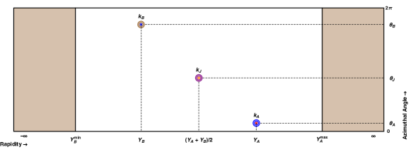
Figure 5.5: A primitive lego plot depicting a three-jet event. $k_{A}$ is a forward jet with large positive rapidity $Y_{A}$ and azimuthal angle $\theta_{A}$, $k_{B}$ is a forward jet with large negative rapidity $Y_{B}$ and azimuthal angle $\theta_{B}$ and $k_{J}$ is a central jet with rapidity $y_{J}$ and azimuthal angle $\theta_{J}$. The fade-brown areas to the left and right highlight the regions in rapidity which are not covered by the standard detectors.

From a more theoretical perspective, it is important to have as good as possible perturbative stability in our predictions (see also Section 5.1.3.1). This can be achieved by removing the contribution stemming from the zero conformal spin, which corresponds to the index $n=0$ in Eqs. (5.15) and (5.27). We, therefore, introduce the ratios

$$R_{PQ}^{MN}\,=\,\frac{C_{MN}}{C_{PQ}}$$ (5.29)

which are free from any $n=0$ dependence, as long as $M,N,P,Q>0$. The postulate that Eq. (5.29) generally describes observables with good perturbative stability is under scrutiny in Sections 5.2.3, 5.2.4, and 5.2.5, where we compare LLA and NLA results.

5.2.2 BLM scale setting

In order to make an appropriate choice of the renormalisation scale $\mu_{R}$, the BLM prescription [BLM, BLM_2, BLM_3, BLM_4, BLM_5] is used. As explained in Section 2.4, it consists of using the MOM scheme and choosing the scale $\mu_{R}$ such that the $\beta_{0}$-dependence of a given observable vanishes. Applying the BLM prescription leads to the modification of the exponent in Eq. (5.27) in the following way:

$$\bar{\alpha}_{s}\left(\chi(n,\nu)+\bar{\alpha}_{s}\chi^{(1)}(n,\nu)\right)Y\,\,\to\,\,\bar{\alpha}_{s}\left(\chi(n,\nu)\left(1+\frac{\alpha_{s}}{\pi}T\right)+\bar{\alpha}_{s}\chi^{(1)}(n,\nu)\right)Y\,,$$ (5.30)

with $T$ given in (2.81). Note that this way to implement BLM is a generalisation of the case (b), given in Eq. (2.87). In the three-jet case, we remove the $\beta_{0}$ dependent factors from the NLA objects present in Eq. (5.23), i.e. the NLA Green’s functions.

Following this procedure, the renormalisation scale $\mu_{R}$ is fixed at the value

$$(\mu_{R}^{\rm BLM})^{2}=k_{A}k_{B}\ \exp\left[\frac{1+4I}{3}+\frac{1}{2}\chi(n,\nu)\right]\,.$$ (5.31)

In our numerical analysis we consider two cases. In one, we set $\mu_{R}=\mu_{R}^{\rm BLM}$ only in the exponential factor of the Green’s function $\varphi_{n}$, while we let the argument of the $\bar{\alpha}_{s}^{3}$ in Eq. (5.23) to be at the “natural” scale $\sqrt{k_{A}k_{B}}$, that is, $\bar{\alpha}_{s}^{3}\sqrt{k_{A}k_{B}}$. In the second case, we fix $\mu_{R}=\mu_{R}^{\rm BLM}$ everywhere in Eq. (5.23). These two cases lead in general to two different but similar values for our NLA predictions and wherever we present plots we fill the space in between so that we end up having a band instead of a single curve for the NLA observables. The band represents the uncertainty that comes into play after using the BLM prescription since there is no unambiguous way to apply it.

5.2.3 Fixed rapidity kinematics for the central jet

In this Section, results for three generalised ratios, $R^{12}_{22}$, $R^{12}_{33}$ and $R^{22}_{33}$ are presented, assuming that the central jet is fixed in rapidity at $y_{J}=(Y_{A}+Y_{B})/2$ (see Fig. 5.5). In particular,

$$C_{MN}=\int_{Y_{A}^{\rm min}}^{Y_{A}^{\rm max}}dY_{A}\int_{Y_{B}^{\rm min}}^{Y_{B}^{\rm max}}dY_{B}\int_{k_{A}^{\rm min}}^{k_{A}^{\rm max}}dk_{A}\int_{k_{B}^{\rm min}}^{k_{B}^{\rm max}}dk_{B}\int_{k_{J}^{\rm min}}^{k_{J}^{\rm max}}dk_{J}\delta\left(Y_{A}-Y_{B}-Y\right){\cal C}_{MN}\;,$$ (5.32)

where the forward jet rapidity is taken in the range delimited by $0<Y_{A}<4.7$, the backward jet rapidity in the range $-4.7<Y_{B}<0$, while their difference $Y\equiv Y_{A}-Y_{B}$ is kept fixed at definite values in the range $5.5<Y<9$.

It is possible to study the ratios $R_{PQ}^{MN}$ in Eq. (5.29) as functions of the rapidity difference Y between the most forward and the most backward jets for a set of characteristic values of $M,N,P,Q$ and for two different center-of-mass energies: $\sqrt{s}=7$ and $\sqrt{s}=13$ TeV. Since we are integrating over $k_{A}$ and $k_{B}$, we have the opportunity to impose either symmetric or asymmetric kinematical cuts, as it has been previously done in Mueller–Navelet studies. Here, and in the next two Sections, we choose to study the asymmetric cut which presents certain advantages over the symmetric one (see Section 3.3 and Refs. [Ducloue:2013wmi, Celiberto:2015yba]). To be more precise, we set $k_{A}^{\rm min}=35$ GeV, $k_{B}^{\rm min}=50$ GeV, $k_{A}^{\rm max}=k_{B}^{\rm max}=60$ GeV throughout the whole analysis.

In order to be as close as possible to the characteristic rapidity ordering of the MRK, we set the value of the central jet rapidity such that it is equidistant to $Y_{A}$ and $Y_{B}$ by imposing the condition $y_{J}=(Y_{A}+Y_{B})/2$. Moreover, since the tagging of a central jet permits us to extract more exclusive information from our observables, we allow three possibilities for the transverse momentum $k_{J}$, that is, $20\,\mathrm{GeV}<k_{J}<35\,\mathrm{GeV}$ (bin-1), $35\,\mathrm{GeV}<k_{J}<60\,\mathrm{GeV}$ (bin-2) and $60\,\mathrm{GeV}<k_{J}<120\,\mathrm{GeV}$ (bin-3). Keeping in mind that the forward/backward jets have transverse momenta in the range $\left[35\,\mathrm{GeV},60\,\mathrm{GeV}\right]$, restricting the value of $k_{J}$ within these three bins allows us to see how the ratio $R_{PQ}^{MN}$ changes behaviour depending on the relative size of the central jet momentum when compared to the forward/backward ones. Throughout the whole Section LABEL:sec:4j-hadronic, we will keep the same setup regarding bin-1, bin-2 and bin-3 which roughly correspond to the cases of $k_{J}$ being ‘smaller’ than, ‘similar’ to and ‘larger’ than $k_{A}$, $k_{B}$, respectively.

Finally, apart from the functional dependence of the ratios on $Y$ we will also show the relative corrections when we go from LLA to NLA. To be more precise, we define

$$\delta x(\%)=\left(\text{res}^{\rm(LLA)}-\frac{\text{res}^{\rm(BLM-1)}+\text{res}^{\rm(BLM-2)}}{2}\right)\frac{1}{\text{res}^{\rm(LLA)}}\,.$$ (5.33)

$\text{res}^{\rm(BLM-1)}$ is the BLM NLA result for $\mu_{R}=\mu_{R}^{\rm BLM}$ only in the Green’s function while the cubed term of the strong coupling in Eq. (5.23) actually reads $\bar{\alpha}_{s}^{3}=\bar{\alpha}_{s}^{3}(\sqrt{k_{A}k_{B}})$). $\text{res}^{\rm(BLM-2)}$ is the BLM NLA result for $\mu_{R}=\mu_{R}^{\rm BLM}$ everywhere in Eq. (5.23), therefore, $\bar{\alpha}_{s}^{3}=\bar{\alpha}_{s}^{3}(\mu_{R}^{\rm BLM})$, as was previously discussed in Section 5.2.1.

In the following, we present our results for $R^{12}_{22}$, $R^{12}_{33}$ and $R^{22}_{33}$, with $y_{J}=(Y_{A}+Y_{B})/2$, collectively in Fig. 5.8 ($\sqrt{s}=7$ TeV) and Fig. 5.9 ($\sqrt{s}=13$ TeV), In the left column we are showing plots for $R^{MN}_{PQ}(Y)$ whereas to the right we are showing the corresponding $\delta x(\%)$ between LLA and NLA corrections. The LLA results are represented with dashed lines whereas the NLA ones with a continuous band. The boundaries of the band are the two different curves we obtain by the two different approaches in applying the BLM prescription. Since there is no definite way to choose one in favour of the other, we allow for any possible value in between and hence we end up with a band. In many cases, as we will see in the following, the two boundaries are so close that the band almost degenerates into a single curve. The red curve (band) corresponds to $k_{J}$ bounded in bin-1, the green curve (band) to $k_{J}$ bounded in bin-2 and finally the blue curve (band) to $k_{J}$ bounded in bin-3. For the $\delta x(\%)$ plots we only have three curves, one for each of the three different bins of $k_{J}$.

A first observation from inspecting Figs. 5.8 and 5.9 is that the dependence of the different observables on the rapidity difference between $k_{A}$ and $k_{B}$ is rather smooth. $R^{12}_{22}$ (top row in Figs. 5.8 and 5.9) at $\sqrt{s}=7$ TeV and for $k_{J}$ in bin-1 and bin-3 exhibits an almost linear behaviour with $Y$ both at LLA and NLA, whereas at $\sqrt{s}=13$ TeV the linear behaviour is extended also for $k_{J}$ in bin-2. The difference between the NLA BLM-1 and BLM-2 values is small, to the point that the blue and the red bands collapse into a single line which in addition lies very close to the LLA results. When $k_{J}$ is restricted in bin-2 (green curve/band), the uncertainty from applying the BLM prescription in two different ways seems to be larger. The relative NLA corrections at both colliding energies are very modest ranging from close to $1\%$ for $k_{J}$ in bin-3 to less than $10\%$ for $k_{J}$ in the other two bins. $R^{12}_{33}$ (middle row in Figs. 5.8 and 5.9) compared to $R^{12}_{22}$, shows a larger difference between BLM-1 and BLM-2 values for $k_{J}$ in bin-1 and bin-2. The ‘green’ corrections lower the LLA estimate whereas the ‘red’ ones make the corresponding LLA estimate less negative. The corrections are generally below $20\%$, in particular, ‘blue’ $\sim 5\%$, ‘red’ $\sim 10\%$ and ‘green’ $\sim 20\%$. Finally, $R^{22}_{33}$ (bottom row in Figs. 5.8 and 5.9) also shows a larger difference between BLM-1 and BLM-2 values for $k_{J}$ in bin-1 and less so for $k_{J}$ in bin-2. Here, the ‘red’ corrections lower the LLA estimate whereas the ‘green’ ones make the corresponding LLA estimate less negative. The corrections are smaller than the ones for $R^{12}_{33}$ and somehow larger than the corrections for $R^{12}_{22}$, specifically, ‘blue’ $\sim 5\%$, ‘red’ $\sim 5\%$ and ‘green’ $\sim 15\%$. Noticeably, while for $R^{12}_{22}$ and $R^{12}_{33}$ the corrections are very similar at $\sqrt{s}=7$ and $\sqrt{s}=13$ TeV, the ‘green’ $R^{22}_{33}$ receives larger corrections at $\sqrt{s}=7$ TeV. One important conclusion we would like to draw after comparing Figs. 5.8 and 5.9 is that, in general, for most of the observables there are no striking changes when we increase the colliding energy from 7 to 13 TeV. This indicates that a sort of asymptotic regime has been approached for the kinematical configurations included in our analysis. It also tells us that our observables are really as insensitive as possible to effects which have their origin outside the BFKL dynamics and which normally cannot be isolated (e.g. influence from the PDFs) with a possible exclusion at the higher end of the plots, when $Y\sim 8.5-9$. There, some of the observables and by that we mean the ‘red’, ‘green’ or ‘blue’ cases of $R^{12}_{22}$, $R^{12}_{33}$ and $R^{22}_{33}$, exhibit a more curved rather than linear behaviour with $Y$ at $\sqrt{s}=7$ TeV.

5.2.4 Dependence of the generalised azimuthal correlations on the central-jet rapidity bin

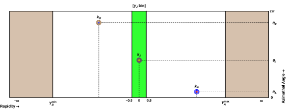
Figure 5.6: A primitive lego plot depicting a three-jet event similar to Fig. 5.5. Here, however, the central jet can take any value in the rapidity range $-0.5<y_{J}<0.5$.

In this Section, everything is kept the same as in Section 5.2.4 with the exemption of the allowed values for $y_{J}$ (see Fig. 5.6). While in the previous Section $y_{J}=(Y_{A}+Y_{B})/2$, here $y_{J}$ is not anymore dependent on the rapidity difference between the outermost jets, $Y$, and is allowed to take values in a rapidity bin around $y_{J}=0$. In particular, $-0.5<y_{J}<0.5$, which in turn means that an additional integration over $y_{J}$ needs to be considered in Eq. (5.32) with $y_{J}^{\rm min}=-0.5$ and $y_{J}^{\rm max}=0.5$:

$$C_{MN}^{\text{(i)}}=\int_{y_{J}^{\rm min}}^{y_{J}^{\rm max}}dy_{J}\int_{Y_{A}^{\rm min}}^{Y_{A}^{\rm max}}dY_{A}\int_{Y_{B}^{\rm min}}^{Y_{B}^{\rm max}}dY_{B}\int_{k_{A}^{\rm min}}^{k_{A}^{\rm max}}dk_{A}\int_{k_{B}^{\rm min}}^{k_{B}^{\rm max}}dk_{B}\int_{k_{J}^{\rm min}}^{k_{J}^{\rm max}}dk_{J}\delta\left(Y_{A}-Y_{B}-Y\right){\cal C}_{MN},$$ (5.34)

We define our observables ${}^{\text{(i)}}R_{PQ}^{MN}$:

$${}^{\text{(i)}}R_{PQ}^{MN}\,=\,\frac{C_{MN}^{\text{(i)}}}{C_{PQ}^{\text{(i)}}}\,.$$ (5.35)

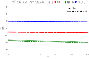
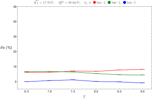
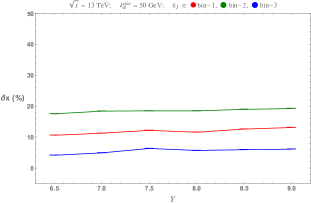
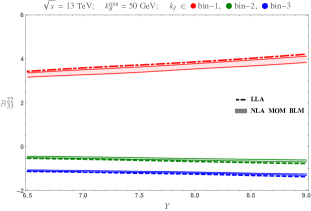
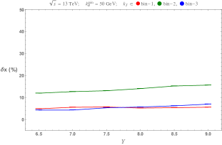
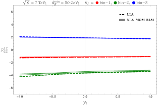
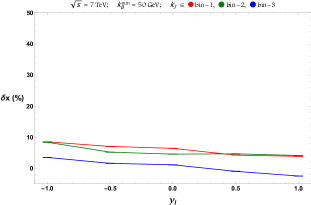
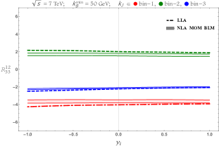
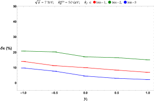
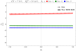
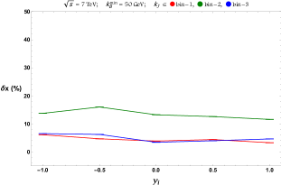
Figure 5.11: LLA and NLA ${}^{\text{(i)}}R^{12}_{22}$, ${}^{\text{(i)}}R^{12}_{33}$, and ${}^{\text{(i)}}R^{22}_{33}$ at $\sqrt{s}=13$ TeV with $y_{J}$ integrated over a central rapidity bin (left) and the relative NLA to LLA corrections (right).

The results for the ${}^{\text{(i)}}R^{12}_{22}$, ${}^{\text{(i)}}R^{12}_{33}$ and ${}^{\text{(i)}}R^{22}_{33}$ are shown in Figs. 5.10 and 5.11. We notice immediately that Fig. 5.8 is very similar to the integrated over $y_{J}$ observables Fig. 5.10 and the same holds for Figs. 5.9 and 5.11. Therefore, we will not discuss here the individual behaviours of $R^{12}_{22}$, $R^{12}_{33}$ and $R^{22}_{33}$ with $Y$, neither the $\delta x(\%)$ corrections, since this would only mean to repeat the discussion of Section 5.2.3. We would like only to note that the striking similarity between Fig. 5.8 and Fig. 5.10 and between Fig. 5.9 and Fig. 5.11 was to be expected if we remember that the partonic-level quantities $\mathcal{R}_{PQ}^{MN}$ do not change noticeably if we vary the position in rapidity of the central jet, as long as the position remains ‘sufficiently’ central (see Ref. [Caporale:2015vya]). This property is very important and we will discuss it more in the next Section. Here, we should stress that the observables as presented in this Section can be readily compared to experimental data.

5.2.5 Dependence of the generalised azimuthal correlations on a forward-, backward- and central-rapidity bin

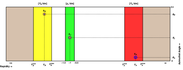
Figure 5.7: A primitive lego plot depicting a three-jet event similar to Figs. 5.5 and 5.6. Here, however, the rapidity of the central jet can take any value in the distinct ranges $y_{i}-0.5<y_{J}<y_{i}+0.5$, where $y_{i}$ is the central value of the rapidity bin with $y_{i}=\{-1,-0.5,0,0.5,1\}$. In this figure, $y_{i}=-1$. Moreover, $Y=Y_{A}-Y_{B}$ is not anymore fixed. Instead, the forward jet has a rapidity restricted in the red bin whereas the backward jet in the yellow bin.

In this Section, an alternative kinematical configuration (see Fig. 5.7) for the generalised ratios $R_{PQ}^{MN}$ is presented, whose choice relies on two reasons. The first one is to offer a different setup for which the comparison between theoretical predictions and experimental data might be easier, compared to the previous Section. The second one, to demonstrate that the generalised ratios do capture the Bethe–Salpeter characteristics [Salpeter:1951sz] of the BFKL radiation. The latter needs a detailed explanation.

Let us assume that we have a gluonic ladder exchanged in the $t$-channel between a forward jet (at rapidity $Y_{A}$) and a backward jet (at rapidity $Y_{B}$) accounting for minijet activity between the two jets. By gluonic ladder here we mean the Green’s function $\varphi\left(\vec{p}_{A},\vec{p}_{B},Y_{A}-Y_{B}\right)$, where $\vec{p}_{A}$ and $\vec{p}_{B}$ are the Reggeised momenta connected to the forward and backward jet vertex respectively. It is known that the following relation holds for the Green’s function:

$$\varphi\left(\vec{p}_{A},\vec{p}_{B},Y_{A}-Y_{B}\right) = \int d^{2}\vec{k}\,\varphi\left(\vec{p}_{A},\vec{k},Y_{A}-y\right)\varphi\left(\vec{k},\vec{p}_{B},y-Y_{B}\right).$$ (5.36)

In other words, one may ‘cut’ the gluonic ladder at any rapidity $y$ between $Y_{A}$ and $Y_{B}$ and then integrate over the Reggeised momentum $\vec{k}$ that flows in the $t$-channel, to recover the initial ladder. Which value of $y$ one chooses to ‘cut’ the ladder at is irrelevant. Therefore, observables directly connected to a realisation of the r.h.s of Eq. (5.36) should display this $y$-independence.

In our study actually, we have a very similar picture as the one described in the r.h.s of Eq. (5.36). The additional element is that we do not only ‘cut’ the gluonic ladder but we also ‘insert’ a jet vertex for the central jet. This means that the $y$-independence we discussed above should be present in one form or another. To be precise, we do see the $y$-independence behaviour but now we have to consider the additional constraint that $y$ cannot take any extreme values, that is, it cannot be close to $Y_{A}$ or $Y_{B}$. For a more detailed discussion of Eq. (5.36), we refer the reader to Appendix D), here we will proceed to present our numerical results.

The kinematical setup now is different than in the previous Sections. We allow $Y_{A}$ and $Y_{B}$ to take values such that $(Y_{A}^{\text{min}}=3)<Y_{A}<(Y_{A}^{\text{max}}=4.7)$ and $(Y_{B}^{\text{min}}=-4.7)<Y_{B}<(Y_{B}^{\text{max}}=-3)$. Moreover, we allow for the rapidity of the central jet to take values in five distinct rapidity bins of unit width, that is, $y_{i}-0.5<y_{J}<y_{i}+0.5$, with $y_{i}=\{-1,-0.5,0,0.5,1\}$ and we define the coefficients $C_{MN}^{\rm(i)}(y_{i})$ as function of $y_{i}$:

$$C_{MN}^{\text{(i)}}(y_{i})=\int_{y_{i}-0.5}^{y_{i}+0.5}dy_{J}\int_{Y_{A}^{\rm min}}^{Y_{A}^{\rm max}}dY_{A}\int_{Y_{B}^{\rm min}}^{Y_{B}^{\rm max}}dY_{B}\int_{k_{A}^{\rm min}}^{k_{A}^{\rm max}}dk_{A}\int_{k_{B}^{\rm min}}^{k_{B}^{\rm max}}dk_{B}\int_{k_{J}^{\rm min}}^{k_{J}^{\rm max}}dk_{J}\,\,{\mathcal{C}}_{MN}.$$ (5.37)

We denote our observables by ${}^{\text{(i)}}R_{PQ}^{MN}$, which are now functions of $y_{i}$ instead of $Y$:

$$R_{PQ}^{MN}(y_{i})\,=\,\frac{C_{MN}^{\text{(i)}}(y_{i})}{C_{PQ}^{\text{(i)}}(y_{i})}\,.$$ (5.38)

We present our results in Figs. 5.12 and 5.13. We see that indeed, the $y_{i}$-dependence of the three ratios is very weak. Moreover, the similarity between the $\sqrt{s}=7$ TeV and $\sqrt{s}=13$ TeV plots is more striking that in the previous Sections. The relative NLA to LLA corrections seem to be slightly larger here than in the previous Sections. We would like to stress once more that the results in this Section are readily comparable to the experimental data once the same cuts are applied in the experimental analysis.

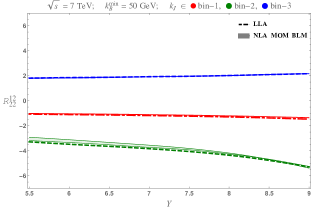
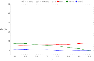
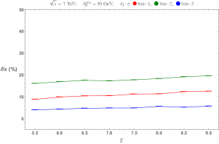
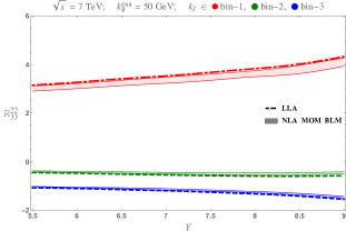
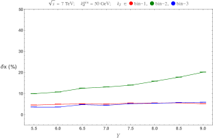
Figure 5.8: LLA and NLA $R^{12}_{22}$, $R^{12}_{33}$, and $R^{22}_{33}$ at $\sqrt{s}=7$ TeV with $y_{J}$ fixed (left) and the relative NLA to LLA corrections (right).

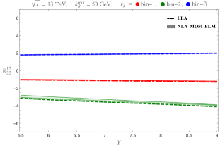
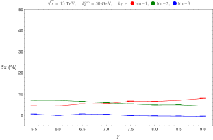
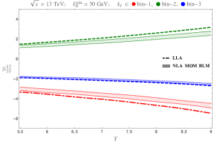
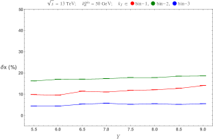
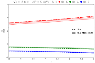
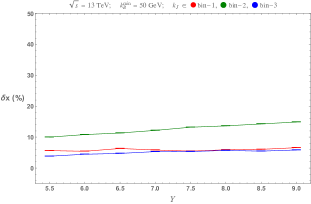
Figure 5.9: $Y$-dependence of the LLA and NLA $R^{12}_{22}$, $R^{12}_{33}$, and $R^{22}_{33}$ at $\sqrt{s}=13$ TeV with $y_{J}$ fixed (left) and the relative NLA to LLA corrections (right).

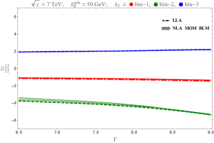
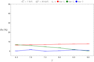
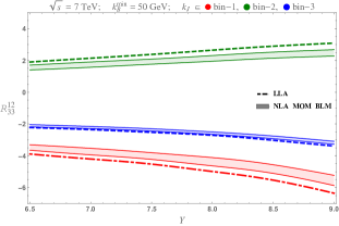
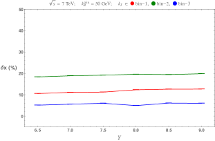
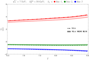
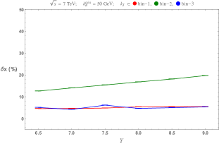
Figure 5.10: LLA and NLA ${}^{\text{(i)}}R^{12}_{22}$, ${}^{\text{(i)}}R^{12}_{33}$, and ${}^{\text{(i)}}R^{22}_{33}$ at $\sqrt{s}=7$ TeV with $y_{J}$ integrated over a central rapidity bin (left) and the relative NLA to LLA corrections (right).

Figure 5.12: $y_{i}$-dependence of the LLA and NLA ${}^{\text{(i)}}R^{12}_{22}(y_{i})$, ${}^{\text{(i)}}R^{12}_{33}(y_{i})$ and ${}^{\text{(i)}}R^{22}_{33}(y_{i})$ at $\sqrt{s}=7$ TeV (left) and the relative NLA to LLA corrections (right).

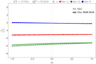
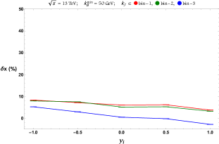
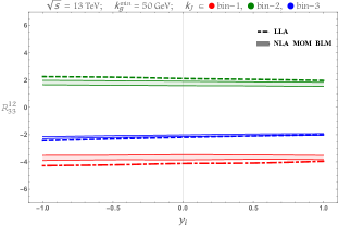
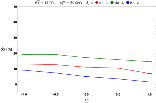
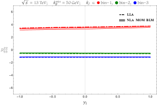
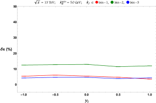
Figure 5.13: $y_{i}$-dependence of the LLA and NLA ${}^{\text{(i)}}R^{12}_{22}$, ${}^{\text{(i)}}R^{12}_{33}$, and ${}^{\text{(i)}}R^{22}_{33}$ at $\sqrt{s}=13$ TeV (left) and the relative NLA to LLA corrections (right).

5.2.6 Numerical tools

The numerical computation of the $\mathcal{R}^{MN}_{PQ}$ ratios presented in Sections 5.2.3, 5.2.4 and 5.2.5 were done both in Fortran and in Mathematica (mainly for cross-checks). The NLO MSTW 2008 PDF sets [Martin:2009iq] were used and a two-loop running coupling setup with $\alpha_{s}\left(M_{Z}\right)=0.11707$ was chosen with five quark flavours active. An extensive use of the integration routine Vegas [VegasLepage:1978] was made, as implemented in the Cuba library [Cuba:2005, ConcCuba:2015]. Furthermore, Quadpack library [Quadpack:book:1983] and a slightly modified version of the Psi [RpsiCody:1973] routine were used.

5.3 Summary

The first complete phenomenological analysis for the inclusive three-jet production was presented. New azimuthal-angle-dependent observables, the $R^{MN}_{PQ}$ ratios, were defined first at the partonic level, then extended and studied at the hadronic level, taking in the account of NLA BFKL corrections. Two colliding energies, $\sqrt{s}=7,13$ TeV, together with an asymmetric kinematical cut with respect to the transverse momentum of the forward ($k_{A}$) and backward ($k_{B}$) jets were considered. In addition, an extra condition regarding the value of the transverse momentum $k_{J}$ of the central jet was taken up, dividing the allowed region for $k_{J}$ into three sub-regions: $k_{J}$ smaller than $k_{A,B}$, $k_{J}$ similar to $k_{A,B}$, and $k_{J}$ larger than $k_{A,B}$.

For a proper study at full NLA, one needs to consider the NLO jet vertices and the NLA Green’s functions, with the latter being expected to be of higher relevance. BLM prescription, which has been successful in previous phenomenological analyses [Khachatryan:2016udy], was used to choose the values of the renormalisation scale $\mu_{R}$. It was shown how the $R^{MN}_{PQ}$ ratios change when we vary the rapidity difference Y between $k_{A}$ and $k_{B}$ from 5.5 to 9 units for a fixed $y_{J}$ and from 6.5 to 9 units for $-0.5<y_{J}<0.5$. Both the LLA and NLA results were presented, along with plots that show the relative size of the NLA corrections compared to the LLA ones. An alternative kinematical setup were also investigated, where $Y_{A}$ and $Y_{B}$ are allowed to take values such that $3<Y_{A}<4.7$ and $-4.7<Y_{B}<-3$, while the rapidity of the central jet takes values in five distinct rapidity bins of unit width, that is, $y_{i}-0.5<y_{J}<y_{i}+0.5$, with $y_{i}=\{-1,-0.5,0,0.5,1\}$. In this alternative setup, we presented the behaviour of our observables as functions of $y_{i}$.

The general conclusion is that the NLA corrections are moderate and our proposed observables exhibit a good perturbative stability. Furthermore, we see that for a wide range of rapidities, the changes we notice when going from $7$ TeV to $13$ TeV are small which makes us confident that these generalised ratios pinpoint the crucial characteristics of the BFKL dynamics regarding the azimuthal behaviour of the hard jets in inclusive three-jet production.

It would be very interesting to have an experimental analysis for these observables using previous and current LHC data. We have the strong belief that such an analysis will help us gauge the applicability of the BFKL dynamics in phenomenological studies at present colliding energies.

Appendix D

$y_{J}$-independent integrated distributions

InthisAppendixitisshownthatEq.(

5.36)isfulfilledinournormalisations.Weintroducethenotationt = lnk^2$towritetheGreen^{\prime}sfunctionintheform\begin{aligned} &\varphi\left(t_{A},t_{B},\theta_{A},\theta_{B},Y\right)\\ =&\frac{e^{-\frac{t_{A}+t_{B}}{2}}}{\pi^{2}}\sum_{n=-\infty}^{\infty}e^{in\left(\theta_{A}-\theta_{B}\right)}\int_{0}^{\infty}d\nu\cos{\left(\nu\left(t_{A}-t_{B}\right)\right)}\,e^{\bar{\alpha}_{s}\chi(n,\nu)Y}\;.\end{aligned}Makinguseof$d k = 12 e^t2 dt$and$k   dk   d θ=