Coalescent-based species tree estimation:
a stochastic Farris transform

Abstract

The reconstruction of a species phylogeny from genomic data faces two significant hurdles: 1) the trees describing the evolution of each individual gene—i.e., the gene trees—may differ from the species phylogeny and 2) the molecular sequences corresponding to each gene often provide limited information about the gene trees themselves. In this paper we consider an approach to species tree reconstruction that addresses both these hurdles. Specifically, we propose an algorithm for phylogeny reconstruction under the multispecies coalescent model with a standard model of site substitution. The multispecies coalescent is commonly used to model gene tree discordance due to incomplete lineage sorting, a well-studied population-genetic effect.

In previous work, an information-theoretic trade-off was derived in this context between the number of loci, $m$, needed for an accurate reconstruction and the length of the locus sequences, $k$. It was shown that to reconstruct an internal branch of length $f$, one needs $m$ to be of the order of $1/[f^{2}\sqrt{k}]$. That previous result was obtained under the molecular clock assumption, i.e., under the assumption that mutation rates (as well as population sizes) are constant across the species phylogeny.

Here we generalize this result beyond the restrictive molecular clock assumption, and obtain a new reconstruction algorithm that has the same data requirement (up to log factors). Our main contribution is a novel reduction to the molecular clock case under the multispecies coalescent. As a corollary, we also obtain a new identifiability result of independent interest: for any species tree with $n\geq 3$ species, the rooted species tree can be identified from the distribution of its unrooted weighted gene trees even in the absence of a molecular clock.

1 Introduction

Modern molecular sequencing technology has provided a wealth of data to assist biologists in the inference of evolutionary relationships between species. Not only is it now possible to quickly sequence a single gene across a wide range of species, but in fact thousands of genes—or entire genomes—can be sequenced simultaneously. With this abundance of data comes new algorithmic and statistical challenges. One such challenge arises because phylogenomic inference entails dealing with the interplay of two processes, as we now explain.

While the tree of life (also referred to as a species phylogeny) depicts graphically the history of speciation of living organisms, each gene within the genomes of these organisms has its own history. That history is captured by a gene tree. In practice, by contrasting the DNA sequences of a common gene across many current species, one can reconstruct the corresponding gene tree. Indeed the accumulation of mutations along the gene tree reflects, if imperfectly, the underlying history. Much is known about the reconstruction of single-gene trees, a subject with a long history; see [SS03a, Fel04, Yan14, Ste16, War] for an overview. The theoretical computer science literature, in particular, has contributed a deep understanding of the computational complexity and data requirements of the problem, under standard stochastic models of sequence evolution on a tree. See, e.g., [GF82, ABF⁺99, FK99, ESSW99a, ESSW99b, Att99, CGG02, SS02, KZZ03, Mos03, Mos04, CT06, Roc06, MR06, BCMR06, MLP09, DMR11a, DMR11b, ADHR12, GMS12, MHR13, DR13, RS].

But a gene tree is only an approximation to the species phylogeny. Indeed various evolutionary mechanisms lead to discordance between gene trees and species phylogenies. These include the transfer of genetic material between unrelated species, hybrid speciation events and a population-genetic effect known as incomplete lineage sorting [Mad97]. The wide availability of genomic datasets has brought to the fore the major impact these discordances have on phylogenomic inference [DBP05, DR09]. As a result, in addition to the stochastic process governing the evolution of DNA sequences on a fixed gene tree, one is led to model the structure of the gene tree itself, in relation to the species phylogeny, through a separate stochastic process. The inference of these complex, two-level evolutionary models is an active area of research. See the recent monographs [HRS10, Ste16, War] for an introduction.

In this paper, we focus on incomplete lineage sorting (from hereon ILS) and consider the reconstruction of a species phylogeny from multiple genes (or loci) under a standard population-genetic model known as the multispecies coalescent [RY03a]. The problem is of great practical interest in computational evolutionary biology and is currently the subject of intense study; see e.g. [LYK⁺09, DR09, ALPE12, Nak13] for a survey. There is in particular a growing body of theoretical results in this area [DR06, DDBR09, DD10, MR10, LYP10, ADR11b, ADR11a, Roc13, DNR14, RS15, DD14, CK15, RW15, MR15, ADR17, SRM], although much remains to be understood. This inference problem is also closely related to another active area of research, the reconstruction of demographic history in population genetics. See e.g. [MFP08, BS14, KMRR15] for some recent theoretical results.

A significant fraction of prior rigorous work on species phylogeny estimation in the presence of ILS has been aimed at the case where “true” gene trees are assumed to be available. However, in reality, one needs to estimate gene trees from DNA sequences, leading to reconstruction errors, and indeed there has been a recent thrust towards understanding the effect of this important source of error in phylogenomic inference, both from empirical [KD07, MBW16] and theoretical [MR10, DD14, RS15, RW15, SRM] standpoints. Another option, which we adopt here, is to bypass the reconstruction of gene trees altogether and infer the species history directly from sequence data [DNR15, MR15, CK15].

In previous work on this latter approach [MR15], an optimal information-theoretic trade-off was derived between the number of genes $m$ needed to accurately reconstruct a species phylogeny and the length of the genes $k$ (which is linked to the quality of the phylogenetic signal that can be extracted from each separate gene). Specifically, it was shown that $m$ needs to scale like $1/[f^{2}\sqrt{k}]$, where $f$ is the length of the shortest branch in the tree (which controls the extent of the ILS). This result was obtained under a restrictive molecular clock assumption, where the leaves are equidistant from the root; in essence, it was assumed that the mutation rates and population sizes do not vary across the species phylogeny, which is rarely the case in practice.

In the current work, we design and analyze a new reconstruction algorithm that achieves the same optimal data requirement (up to log factors) beyond the molecular clock assumption. Our key contribution is of independent interest: we show how to transform sequence data to appear as though it was generated under the multispecies coalescent with a molecular clock. We achieve this through a novel reduction which we call a stochastic Farris transform. Our construction relies on a new identifiability result: for any species phylogeny with $n\geq 3$ species, the rooted species tree can be identified from the distribution of the unrooted weighted gene trees even in the absence of a molecular clock.

We state our main results formally in Section 2 and describe our new reduction in Section 3. The proofs are in Sections B, C, D and E.

2 Background and main results

In this section, we state formally our main results and provide a high-level view of the proof.

2.1 Basic definitions

We begin with a brief description of our modeling assumptions. More details on the models, which are standard in the phylogenetic literature (see e.g. [Ste16]), are provided in Section A.

Species phylogeny v. gene trees

A species phylogeny is a graphical depiction of the evolutionary history of a set of species. The leaves of the tree correspond to extant species while internal vertices indicate a speciation event. Each edge (or branch) corresponds to an ancestral population and will be described here by two numbers: one that indicates the amount of time that the corresponding population lived, and a second one that specifies the rate of genetic mutation in that population. Formally, we define the species phylogeny (or tree) as follows.

Definition 1 (Species phylogeny).

A species phylogeny $S=(V_{s},E_{s};r,\vec{\tau},\vec{\mu})$ is a directed tree rooted at $r\in V_{s}$ with vertex set $V_{s}$, edge set $E_{s}$, and $n$ labelled leaves $L=\left\{1,2,\ldots,n\right\}$ such that (a) the degree of all internal vertices is $3$ except for the root $r$ which has degree $2$, and (b) each edge $e\in E_{s}$ is associated with a length $\tau_{e}\in(0,\infty)$ and a mutation rate $\mu_{e}\in(0,\infty)$.

To be more precise, as is standard in coalescent theory (see, e.g., [Ste16]), the length $\tau_{e}$ of a branch $e\in E_{s}$ is expressed in coalescent time units, which is the duration of the branch $t_{e}$ divided by its population size $N_{e}$. That is, $\tau_{e}=t_{e}/N_{e}$. We pictorially represent species phylogenies as thick shaded trees; see Fig. 1 for an example with $n=3$ leaves.

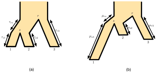
Figure 1: (a) A species phylogeny with $n=3$ leaves $\{1,2,3\}$ and two internal vertices $r$ and $s$. The branch lengths are denoted by $\{\tau_{s1},\tau_{s2},\tau_{rs},\tau_{r3}\}$. Depicted above is the special case where all population sizes are the same, in which case the species phylogeny is “ultrametric,” that is, all leaves are the same distance from the root under $\vec{\tau}$. (b) The same phylogeny with branches stretched by the corresponding mutation rates. The mutation rate-weighted branch lengths are denoted by $\{\mu_{s1},\mu_{s2},\mu_{rs},\mu_{r3}\}$, with respect to which ultrametricity is in general lost—our focus here.

While a species phylogeny describes the history of speciation, each gene has its own history which is captured by a gene tree.

Definition 2 (Gene trees).

A gene tree $G^{(i)}=(V^{(i)},E^{(i)};r,\vec{\delta}^{(i)})$ corresponding to gene $i$ is a directed tree rooted at $r$ with vertex set $V^{(i)}$ and edge set $E^{(i)}$, and the same labeled leaf set $L=\left\{1,2,\ldots,n\right\}$ as $S$ such that (a) the degree of each internal vertex is $3$, except the root $r$ whose degree is $2$, and (b) each branch $e\in E^{(i)}$ is associated with a branch length $\delta_{e}^{(i)}\in(0,\infty)$.

In essence, these gene trees “evolve” on the species phylogeny. More specifically, following [RY03b], we assume that a multispecies coalescent (MSC) process produces $m$ independent random gene trees $G^{(1)},G^{(2)},\ldots,G^{(m)}$. This process is parametrized by the species phylogeny $S$. In words, proceeding backwards in time, in each population, every pair of lineages entering from descendant populations merge at a unit exponential rate. We describe this process formally in Algorithm 4 in Section A. For the present discussion, it suffices to think of the MSC as a random process generating “noisy versions” of the species phylogeny. We highlight one key feature of the gene trees: their topology may be distinct from that of the species phylogeny. This discordance, which in this context is referred to as incomplete lineage sorting (see e.g. [DR09]), is a major challenge for species tree estimation from multiple genes. See Figure 2 for an illustration in the case $n=3$.

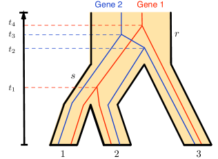
Figure 2: Two sample draws from the MSC on a species phylogeny with $n=3$ leaves. The (rooted) topology of Gene 1 (red gene) agrees with the topology of the underlying species phylogeny (i.e., species $1$ and $2$ are closest), while the topology of Gene 2 (blue gene) does not (here species $2$ and $3$ are closest instead).

Sequence data and inference problem

The gene trees are not observed directly. Rather, they are typically inferred from sequence data “evolving” on the gene trees. We model this sample generation process according to the standard Jukes-Cantor (JC) model (see, e.g., [Ste16]). That is, given a gene tree $G^{(i)}=(V^{(i)},E^{(i)};r,\vec{\delta}^{(i)})$, we associate to each $e\in E^{(i)}$, a probability

$$p_{e}^{(i)}=\frac{3}{4}\left(1-e^{-\frac{4}{3}\delta_{e}^{(i)}}\right),$$

where $\delta_{e}^{(i)}$ is the mutation rate-weighted edge length. In words, the corresponding gene $i$ is a sequence of length $k$ in $\left\{{\tt A,T,G,C}\right\}^{k}$. Each position in the sequence evolves independently, starting from a uniform state in $\left\{{\tt A,T,G,C}\right\}$ at the root. Moving away from the root, a substitution occurs on edge $e$ with probability $p_{e}^{(i)}$, in which case the state changes to state chosen uniformly among the remaining states. After repeating this process for all positions, one obtains a sequence of length $k$ for each leaf of $G^{(i)}$, for each $i\in[m]$—that is our input. A full algorithmic description of the Jukes-Cantor process is provided as Algorithm 3 in Section A.

For gene $i$, we will let $\left\{\xi^{ij}_{x}\,:\,j\in[k],x\in L\right\}$ denote the data generated at the leaves $L$ of the tree $G^{(i)}$ per the Jukes-Cantor process, the superscript $j$ runs across the positions of the gene sequence. To simplify the notation, we denote $\xi^{ij}=(\xi^{ij}_{x})_{x\in L}$. The species phylogeny estimation problem can then be stated as follows:

The $n\times m\times k$ data array $\left\{\xi^{ij}\right\}_{i\in[m],j\in[k]}$ is generated according to the Jukes-Cantor process on the $m$ gene trees, each of which in turn is generated according to the multi-species coalescent on $S$. The goal is to recover the topology of the species phylogeny $S$ from $\left\{\xi^{ij}\right\}_{i\in[m],j\in[k]}$.

We abbreviate this two-step data generation process by saying that $\left\{\xi^{ij}\right\}_{i\in[m],j\in[k]}$ is generated according to the MSC-JC$(m,k)$ process on $S$.

2.2 Main result

Algorithm 1 Quantile-based triplet test

1:Sequence output by Algorithm 2 $\{\xi_{x,N}^{ij}\,:\,x\in\mathcal{X}=\left\{1,2,3\right\},i\in\mathcal{M}_{{\rm Q}},j\in[k]\}$. A partition of the set of genes $[m]=\mathcal{M}_{{\rm R}}\sqcup\mathcal{M}_{{\rm Q}}$, where $\mathcal{M}_{{\rm R}}=\mathcal{M}_{{\rm R}1}\sqcup\mathcal{M}_{{\rm R}2}$ and $\mathcal{M}_{{\rm Q}}=\mathcal{M}_{{\rm Q}1}\sqcup\mathcal{M}_{{\rm Q}2}$ satisfy the conditions of Proposition 3.

2:For each $x,y\in\mathcal{X}$ and $i\in\mathcal{M}_{{\rm Q}}$, let $\widehat{q}_{xy}^{i}=\sum_{j=1}^{k}\mathbbm{1}\{\xi_{x,N}^{ij}\neq\xi_{y,N}^{ij}\}$.

3:Set $\alpha\triangleq\max\left\{m^{-1}\log m,k^{-0.5}\sqrt{\log k}\right\}$, and partition $\mathcal{M}_{{\rm Q}}=\mathcal{M}_{{\rm Q}1}\sqcup\mathcal{M}_{{\rm Q}2}$ such that $\left|\mathcal{M}_{{\rm Q}1}\right|,\left|\mathcal{M}_{{\rm Q}2}\right|$ satisfy the conditions in Proposition 3.

4:Ultrametric Quantile Test on $\left\{\widehat{q}_{xy}^{i}:{x,y\in\mathcal{X},i\in\mathcal{M}_{{\rm Q}1}}\right\}$

5:For each pair of leaves $x,y\in\mathcal{X}$, compute $\widehat{q}^{(c_{3}\alpha)}_{xy}$, the $c_{3}\alpha$-th quantile with respect to the data $\left\{\widehat{q}_{xy}^{i}:i\in\mathcal{M}_{{\rm Q}1}\right\}$. The constant $c_{3}$ is as in Proposition 7. Define

$$\widehat{q}_{\ast}\triangleq\max_{x,y\in\left\{1,2,3\right\}}\widehat{q}^{(c_{3}\alpha)}_{xy}.$$

6:Next, for $x,y\in\mathcal{X}$, define a similarity measure

$$\widehat{s}_{xy}\triangleq\frac{1}{\left|\mathcal{M}_{{\rm Q}2}\right|}\left|\left\{i\in\mathcal{M}_{{\rm Q}2}:\widehat{q}^{i}_{xy}\leq\widehat{q}_{\ast}\right\}\right|.$$

7:Return Declare that the topology is $xy|z$ if $\widehat{s}_{xy}>\max\left\{\widehat{s}_{xz},\widehat{s}_{yz}\right\}.$

Algorithm 2 Reduction step

1:Sequences $\{\xi_{x}^{ij}\,:\,x\in\mathcal{X}=\left\{1,2,3\right\},i\in[m],j\in[k]\}$. A partition of the set of genes $[m]=\mathcal{M}_{{\rm R}}\sqcup\mathcal{M}_{{\rm Q}}$, where $\mathcal{M}_{{\rm R}}=\mathcal{M}_{{\rm R}1}\sqcup\mathcal{M}_{{\rm R}2}$ and $\mathcal{M}_{{\rm Q}}=\mathcal{M}_{{\rm Q}1}\sqcup\mathcal{M}_{{\rm Q}2}$ satisfy the conditions of Proposition 3.

2:For each $x,y\in\mathcal{X}$ and $i\in\mathcal{M}_{{\rm R}}$, define $\widehat{p}_{xy}^{i}=\frac{1}{k}\sum_{j=1}^{k}\mathbbm{1}\{\xi^{ij}_{x}\neq\xi^{ij}_{y}\}$, $\widehat{p}^{i\downarrow}_{xy}=\frac{2}{k}\sum_{j=1}^{k/2}\mathbbm{1}\{\xi^{ij}_{x}\neq\xi^{ij}_{y}\}$, and $\widehat{p}^{i\uparrow}_{xy}=\frac{2}{k}\sum_{j=k/2+1}^{k}\mathbbm{1}\{\xi^{ij}_{x}\neq\xi^{ij}_{y}\}$.

3:Let $\{x_{i},y_{i}\}$, $i=1,2,3$, be the three distinct (unordered) pairs of distinct leaves in $\mathcal{X}$.

4:for i = 1,2 do

5: Fixing gene tree topologies

6:   Let $x=x_{i}$ and $y=y_{i}$.

7:   Let $z$ be the unique element in $\mathcal{X}-\{x,y\}$.

8:   Compute the empirical quantiles $\widehat{p}_{xy}^{(1/3)}$, $\widehat{p}_{xz}^{(2/3)}$, $\widehat{p}_{xz}^{(5/6)}$, $\widehat{p}_{yz}^{(2/3)}$, and $\widehat{p}_{yz}^{(5/6)}$ from the loci in $\mathcal{M}_{{\rm R}1}$. For instance, to compute $\widehat{p}_{xy}^{(1/3)}$, sort the set $\left\{\widehat{p}^{i}_{xy}:i\in\mathcal{M}_{{\rm R}1}\right\}$ in ascending order and pick the $\left\lfloor\frac{\left|\mathcal{M}_{{\rm R}1}\right|}{3}\right\rfloor$-th element, breaking ties arbitrarily.

9:   Set $I:=\left\{i\in\mathcal{M}_{{\rm R}2}:\widehat{p}_{xy}^{i\downarrow}\leq\widehat{p}_{xy}^{(1/3)},\widehat{p}_{xz}^{(2/3)}\leq\widehat{p}_{xz}^{i\downarrow}\leq\widehat{p}_{xz}^{(5/6)},\widehat{p}_{yz}^{(2/3)}\leq\widehat{p}_{yz}^{i\downarrow}\leq\widehat{p}_{yz}^{(5/6)}\right\}$.

10: Estimation of differences $\Delta_{xy}$

11:   Set $\widehat{p}^{I}_{xz}:=\frac{1}{\left|I\right|}\sum_{i\in I}\widehat{p}_{xz}^{i\uparrow}$, and similarly for $\widehat{p}_{yz}^{I}$.

12:   Set $\widehat{\Delta}_{xy}:=-\widehat{\Delta}_{yx}:=-\frac{3}{4}\log\left(\frac{1-\frac{4}{3}\widehat{p}_{yz}^{I}}{1-\frac{4}{3}\widehat{p}_{xz}^{I}}\right)$

13:end for

14:Let $z_{3}$ be the unique element in $\mathcal{X}-\{x_{3},y_{3}\}$.

15:Set $\widehat{\Delta}_{x_{3}y_{3}}:=\widehat{\Delta}_{x_{3}z_{3}}-\widehat{\Delta}_{y_{3}z_{3}}$.

16:Stochastic Farris transform

17:Find a permutation $\{x,y,z\}$ of $\mathcal{X}$ such that $\min\{\widehat{\Delta}_{zx},\widehat{\Delta}_{zy}\}\geq 0$.

18:For each gene $i\in\mathcal{M}_{{\rm Q}}$ and $j\in[k]$, set $\xi_{z,N}^{ij}=\xi^{ij}_{z}$. Also set $\xi_{x,N}^{ij}=\xi^{ij}_{x}$ with probability $1-p(\widehat{\Delta}_{zx})$ and otherwise choose $\xi_{x,N}^{ij}$ uniformly from $\{{\tt A,T,G,C}\}\setminus\xi^{ij}_{x}$. Do the same to $\xi^{ij}_{y}$ (with $\widehat{\Delta}_{yz}$ instead of $\widehat{\Delta}_{xz}$) to obtain $\xi^{ij}_{y,N}$.

19:Return “noisy” sequence data $\left\{\xi^{ij}_{x,N}:i\in\mathcal{M}_{{\rm Q}},j\in[k],x\in\mathcal{X}\right\}$

We now state our main result for the species phylogeny estimation problem. For any 3 leaves $x,y,z\in L$, the species phylogeny $S$ restricted to these three leaves has one of three possible rooted topologies: $xy|z$, $xz|y$, or $yz|x$. For instance, $12|3$ is depicted in Figure 1 (a) and indicates that $1$ and $2$ are closest. It is a classical phylogenetic result that if one is able to correctly reconstruct the topology of all triples of leaves in $L$, then the topology of the full species phylogeny can be correctly reconstructed as well (see e.g., [Ste16]). Therefore, to simplify the presentation, in what follows our algorithms and theoretical guarantees are stated for a fixed triple $\mathcal{X}=\{1,2,3\}$ (without loss of generality) among the set of leaves $L$.

Our main contribution is a novel polynomial-time reconstruction algorithm for the species phylogeny estimation problem, along with a rigorous data requirement which is optimal (up to log factors) by the work of [MR15]. Moreover, unlike [MR15], our results hold when mutation rates and populations sizes are allowed to vary across the species phylogeny. Our reconstruction algorithm comprises two steps, which are detailed as Algorithm 1 and Algorithm 2. Our data requirement applies to an unknown species phylogeny in the following class. We assume that: mutation rates are in the interval $(\mu_{L},\mu_{U})$; leaf-edge lengths are in $(f^{\prime},g^{\prime})$; and internal-edge lengths are in $(f,g)$. We suppress the dependence on $\mu_{L},\mu_{U},f^{\prime},g^{\prime},g$, which we think of as constants, and focus here on the role of $f$. The latter indeed plays a critical role in both the random processes described above. Short internal branches are known to be hard to reconstruct from sequence data even when dealing with a single gene tree [SS02] and a smaller $f$ also leads to more discordance between gene trees [RY03b]. We also suppress the dependence on the number of leaves $n=|L|$, which we also consider here to be a constant (see the concluding remarks in Section 4 for more on this).

We state here a simplified version of our results (the more general statement appearing as Proposition 3 in Section C). Specifically, we answer the following question: as $f\to 0$, how many genes $m$ of length $k$ are needed for a correct reconstruction with high probability? For technical reasons, our results apply only when $k$ grows at least polynomially with $f$ (with an arbitrarily small exponent). Throughout, we use the notation $\gtrsim$ (similarly, $\lesssim$) to indicate that constants and $\text{poly}(\log f^{-1})$ factors are suppressed in a lower bound. Recall that $x\lor y=\max\{x,y\}$.

Theorem 1 (Data requirement).

Suppose that we have sequence data $\left\{\xi^{ij}\right\}_{i\in[m],j\in[k]}$ generated according to the MSC-JC$(m,k)$ process on a species phylogeny $S=(V_{s},E_{s};r,\vec{\tau},\vec{\mu})$ . The mutation rates, leaf-edge lengths and internal-edge lengths are respectively in $(\mu_{L},\mu_{U})$, $(f^{\prime},g^{\prime})$ and $(f,g)$. We assume further that there is $C>0$ such that $k\gtrsim f^{-C}$. Then Algorithm 1 correctly identifies the topology of $S$ restricted to $\mathcal{X}=\{1,2,3\}$ with probability at least $95\%$ provided that

$$m\gtrsim\frac{1}{f}\lor\frac{1}{\sqrt{k}f^{2}}.$$ (1)

Two regimes are implicit in Theorem 1:

• “Long” sequences: When $k\gtrsim f^{-2}$, we require $m\gtrsim f^{-1}$. As first observed by [MR10], this condition is always required for high-probability reconstruction under this setting.

• “Short” sequences: When $k\lesssim f^{-2}$, we require the stronger condition that $m\gtrsim k^{-1/2}f^{-2}$. This is known to be optimal (up to the log factor) by the information-theoretic lower bound in [MR15]. As mentioned above, the matching algorithmic upper bound of [MR15] only applies when all mutation rates and population sizes are identical. Our main contribution here is to relax this assumption.

On the other hand, our results do not apply to the regime of “very short” sequences of constant length. In that regime, the reconstruction algorithm of [DNR15], which applies under the same setting we are considering here, achieves the optimal bound of $m\gtrsim f^{-2}$.

2.3 Proof idea and further results

We give a brief overview of the proof. The full details are given in Section 3 as well as Sections C, D and E. Again, fix a triple of leaves $\mathcal{X}=\{1,2,3\}$.

Tree metrics

Phylogenies are naturally equipped with a notion of distance between leaves, and in general any pair of vertices, which is known as a tree metric (see e.g. [Ste16] for more details). Our species phylogeny reconstruction method rests on such tree metrics.

Definition 3 (Weighted species metric).

A species phylogeny $S=(V_{s},E_{s};r,\vec{\tau},\vec{\mu})$ induces the following metric on the leaf set $L$. For any pair of leaves $a,b\in L$, we let

$$\mu_{ab} =\sum_{e\in\pi(a,b;S)}\tau_{e}\,\mu_{e},$$

where $\pi(a,b;S)$ is the unique path connecting $a$ and $b$ in $S$ interpreted as a set of edges. We will refer to $\left\{\mu_{ab}\right\}_{a,b\in L}$ as the weighted species metric induced by $S$.

The above definition is valid for any pair of vertices in $V_{s}$. That is, the metric $\mu$ can be extended to the entire set $V_{s}$. In the species phylogeny estimation problem, the sequence data only carries information about the rate-weighted distances $\left\{\mu_{ab}\right\}_{a,b\in L}$. The algorithm in [MR15] is guaranteed to recover the topology of $S$ only in the case that $\left\{\mu_{ab}\right\}_{a,b\in L}$ is an ultrametric on the leaf set $L$, in which case we refer to $S$ as an ultrametric species phylogeny. The metric $\left\{\mu_{ab}\right\}_{a,b\in L}$ is ultrametric when $\mu_{ra}=\mu_{rb}$ for all $a,b\in L$, that is, when the distance from the root to every leaf is the same.

Recall from Definition 2 that each each random gene tree has an associated set of branch lengths. From the description of the multispecies coalescent (see Section A), it follows that a single branch of a gene tree may span across multiple branches of the species phylogeny; this can also be seen in Fig. 2. Let $t_{\tilde{e}}$ denote the (random) length of the branch $\tilde{e}\in E^{(i)}$. For any species phylogeny branch $e\in E_{s}$, let $t_{\tilde{e}\cap e}$ denote the length of the branch $\tilde{e}$ that overlaps with $e$. Then, $\delta_{\tilde{e}}$ and $t_{\tilde{e}}$ satisfy the following relationship

$$\delta_{\tilde{e}}=\sum_{e\in E_{s}}\mu_{e}t_{\tilde{e}\cap e}.$$

This set of weights again defines a different metric on the leaves $L$ of the species tree.

Definition 4 (Gene metric).

A gene tree $G^{(i)}=(V^{(i)},E^{(i)};r,\vec{\delta}^{(i)})$ induces the following metric on the leaf set $L$. For any pair of leaves $a,b\in L$, we (overload the notation $\delta$) and let

$$\delta_{ab}^{(i)} =\sum_{e\in\pi(a,b;G^{(i)})}\delta_{e}^{(i)}$$

where, again, $\pi(a,b;G^{(i)})$ is the unique path connecting $a$ and $b$ in $G^{(i)}$ interpreted as a set of edges. We will refer to $\left\{\delta_{ab}^{(i)}\right\}_{a,b\in L}$ as the gene metric induced by $G^{(i)}$.

Note that, when the species phylogeny $S$ is ultrametric, so are the gene trees.

Ultrametric reduction

At a high level, our reconstruction algorithm relies on a quantile triplet test developed in [MR15]. Roughly speaking this test, which is detailed in Algorithm 1, compares a well-chosen quantile of the sequence-based estimates of gene metrics $\left\{\delta_{ab}^{(i)}\right\}_{a,b\in\mathcal{X}}$ in order to determine which pair of leaves is closest. The algorithm of [MR15], however, only works when all mutation rates and population sizes are equal. In that case, the species phylogeny and gene trees are ultrametric, as defined above. That property leads to symmetries that play a crucial role in the algorithm. Our first main contribution here is a reduction to the this ultrametric case.

That is, in order to apply the quantile triplet test, we first transform the sequence data to appear as though it was was generated by an ultrametric species phylogeny. This ultrametric reduction, inspired by a classical technique known as the Farris transform (see e.g. [SS03b]), may be of independent interest as it could be used to generalize other reconstruction algorithms. Formally, we prove the following theorem. Again, we state a simplified version of our result which gives a lower bound on the number of genes $m$ of length $k$ needed to achieve a desired accuracy (the more general statement appearing as Proposition 4 in Section D). More specifically, Algorithm 2 takes as input two sets of genes, $\mathcal{M}_{{\rm R}}$ and $\mathcal{M}_{{\rm Q}}$. The set $\mathcal{M}_{{\rm R}}$ is used to estimate parameters needed for the reduction. The reduction is subsequently performed on $\mathcal{M}_{{\rm Q}}$. We let $m^{\prime}=|\mathcal{M}_{{\rm R}}|$. Here we give a lower bound on $m^{\prime}$ (while, for the purposes of this theorem, $|\mathcal{M}_{{\rm Q}}|$ can be arbitrarily large). For $\theta>0$, we say that two metrics $\mu^{\prime}$ and $\mu^{\prime\prime}$ over $\mathcal{X}$ are $\theta$-close if $\left|\mu^{\prime}_{xy}-\mu^{\prime\prime}_{xy}\right|\leq\theta$, for all $x,y\in\mathcal{X}$.

Theorem 2 (Ultrametric reduction).

Suppose that we have sequence data $\left\{\xi^{ij}\right\}_{i\in[m],j\in[k]}$ generated according to the MSC-JC$(m,k)$ process on a three-species phylogeny $S=(V_{s},E_{s};r,\vec{\tau},\vec{\mu})$. The mutation rates, leaf-edge lengths and internal-edge lengths are respectively in $(\mu_{L},\mu_{U})$, $(f^{\prime},g^{\prime})$ and $(f,g)$. We assume further that there is $C>0$ such that $k\gtrsim f^{-C}$. Then, with probability at least $95\%$, the output of Algorithm 2 is distributed according to the MSC-JC process on a species tree $S^{\prime}$ that is $\phi$-close to an ultrametric species phylogeny with rooted topology identical to that of $S$ restricted to $\mathcal{X}=\{1,2,3\}$, provided that

$$m^{\prime}\gtrsim 1\lor\frac{1}{kf^{2}},$$ (2)

where $\phi=\Theta(f/\log f^{-1})$.

The log factor in $\phi$ is needed in our analysis of the quantile test below. The key to the proof of Theorem 2 is the establishment of a new identifiability result of independent interest.

Theorem 3 (Identifiability of rooted species tree from unrooted weighted gene trees).

Let $S=(V_{s},E_{s};r,\vec{\tau},\vec{\mu})$ be a species tree with $n\geq 3$ leaves and root $r$ and let $G=(V,E;r,\vec{\delta})$ be a sampled gene tree from the MSC with branch lengths $\delta_{e}$, $e\in E$. Then the rooted topology of the species tree $S$ is identifiable from the distribution of the unrooted weighted gene tree $G$.

The case $n\geq 5$ is not new. Indeed, it follows from [ADR11b, Theorem 9], where it is shown that in fact the distribution of the unrooted gene tree topologies (without any branch length information) suffices to identify the rooted species phylogeny when the number of leaves exceeds 4. On the other hand, it was also shown in [ADR11b, Proposition 3] that, when $n=4$, the gene tree topologies are not enough to locate the root of the species phylogeny (and the case $n=3$ is trivial). Here we show that, already with three species (and therefore also when $n>3$), the extra information in the gene tree branch lengths allows to recover the root. We give a constructive proof of Theorem 3, which we then adapt to obtain Algorithm 2. More details on this key step are given in Section 3.

Robustness of quantile test

Algorithm 2 produces a new sequence dataset $\left\{\xi_{x,N}^{ij}:x\in\mathcal{X}\right\}$ that appears close to being distributed according to an ultrametric species phylogeny. The next step is to perform a triplet test of [MR15], detailed in Algorithm 1. Roughly speaking, this test is based on comparing an appropriately chosen quantile of the gene metrics. In fact, because we do not have direct access to the latter, we use a sequence-based surrogate, the empirical $p$-distances

$$\widehat{q}^{i}_{xy}=\frac{1}{k}\sum_{j=1}^{k}\mathbbm{1}\left\{\xi_{x,N}^{ij}\neq\xi_{y,N}^{ij}\right\},$$

for each gene $i\in\mathcal{M}_{{\rm Q}}$ in the output of the reduction, whose expectation is a monotone transformation of the corresponding gene metrics. The idea of Algorithm 1 is to use the above $p$-distances to define a “similarity measure” $\widehat{s}_{xy}$ between each pair of leaves $x,y\in\mathcal{X}$ to reveal the underlying species tree topology on $\mathcal{X}$. It works as follows. The set of genes $\mathcal{M}_{{\rm Q}}$ is divided into two disjoint subsets $\mathcal{M}_{{\rm Q}1},\mathcal{M}_{{\rm Q}2}$. The set $\mathcal{M}_{{\rm Q}1}$ is used to compute the $c_{3}\alpha$-quantile $\widehat{q}^{(c_{3}\alpha)}_{xy}$ of $\{\widehat{q}^{i}_{xy}\,:\,i\in\mathcal{M}_{{\rm Q}1}\}$, where $c_{3}>0$ is a constant determined in the proofs and

$$\alpha=\max\left\{\frac{\log m}{m},\sqrt{\frac{\log k}{k}}\right\}.$$

Let $\widehat{q}_{\ast}$ denote the maximum among $\left\{\widehat{q}^{(c_{3}\alpha)}_{xy}:x,y\in\mathcal{X}\right\}$. We then use the genes in $\mathcal{M}_{{\rm Q}2}$ to define the similarity measure

$$\widehat{s}_{xy}=\frac{1}{\left|\mathcal{M}_{{\rm Q}2}\right|}\left|\left\{i\in\mathcal{M}_{{\rm Q}2}:\widehat{q}^{i}_{xy}\leq\widehat{q}_{\ast}\right\}\right|.$$

Whichever pair $x,y\in\mathcal{X}$ produces the largest value of $\widehat{s}_{xy}$ is declared the closest, i.e., the output is $xy|z$ where $z$ is the remaining leaf in $\mathcal{X}$.

Why does it work? Intuitively, the closest pair of species $x,y$ will tend to produce a larger number of genes with few differences between their sequences at $x$ and $y$, as measured by the $p$-distance. In fact it was shown in [MR10] that, under the MSC-JC process on an ultrametric phylogeny when sequences are long enough (namely $k\gtrsim f^{-2}$), choosing the pair of species achieving the smallest $p$-distance across genes succeeds with high probability under optimal data requirements. When $k$ is short on the other hand (namely $k\lesssim f^{-2}$), the randomness from the JC process produces outliers that confound this approach. To make the test more robust, it is natural to turn to quantiles, i.e., to remove a small, fixed fraction of outliers. On a fixed gene tree, the standard deviation of the $p$-distance is of order $1/\sqrt{k}$. It was shown in [MR15] that, as a result, $1/\sqrt{k}$ is in a sense the smallest quantile that can be meaningfully controlled and that it leads to a successful test under optimal data requirements. Our choice of quantile $\alpha$ is meant to cover both regimes above simultaneously. See [MR15], as well as [MR10, DNR15], for more details.

As stated in Theorem 2, the output to the ultrametric reduction is almost—but not perfectly—ultrametric. In our second main contribution, to account for this extra error, we perform a delicate robustness analysis of the quantile-based triplet test. This step is detailed in Section E. At a high level, the proof follows [MR15]. After 1) controlling the deviation of the quantiles, we establish that 2) the test works in expectation and then 3) finish off with concentration inequalities. All these steps must be updated to account for the error introduced in the reduction step. Step 2) is particularly involved and requires the delicate analysis of the CDF of a mixture of binomials.

3 Key ideas in the ultrametric reduction

The goal of the ultrametric reduction step, Algorithm 2, is to transform the sequence data to appear statistically as though it is the output of an MSC-JC process on an ultrametric species phylogeny with the same topology as $S$ restricted to $\mathcal{X}$.

3.1 Preliminary step: a new identifiability result

Before diving into the description of Algorithm 2, we provide some insights into the algebra of our reduction by first deriving a new identifiability result, Theorem 3. That is, we show that, under the multispecies coalescent, the rooted topology of the species phylogeny can be recovered from the distribution of the unrooted weighted gene trees.

Our reduction is inspired by the Farris transform (also related to the Gromov product; see e.g. [SS03b]), a classical technique to transform a general metric into an ultrametric. In a typical application of the Farris transform, one “roots” the species phylogeny $S$ at an “outgroup” $o$ (i.e., a species that is “far away” from the leaves of $S$) and then uses the quantities $\mu_{ox},x\in L$ to implicitly stretch the leaf edges appropriately, so as to make all inter-species distances to $o$ equal, without changing the underlying topology. More specifically, let $S$ be a species phylogeny. Suppose $\mathcal{X}=\{1,2,3\}$ and let $o\in L-\mathcal{X}$ be any leaf of $S$ outside $\mathcal{X}$. Assume that $\mu_{o1}\geq\max\{\mu_{o2},\mu_{o3}\}$ (the other cases being similar) and define the Farris transform

$$\dot{\mu}_{xy}\triangleq\mu_{xy}+2\mu_{o1}-\mu_{ox}-\mu_{oy},\qquad\forall x,y\in\mathcal{X}.$$ (3)

A classical phylogenetic result (proved for instance in [SS03a, Lemma 7.2.2]) states that $\{\dot{\mu}_{xy}\}_{x,y\in\mathcal{X}}$ is an ultrametric on $\mathcal{X}$ consistent with the topology of $S$ re-rooted at $o$ and, then, restricted to $\mathcal{X}$.

In the multi-gene context, however, we cannot apply a Farris transform in this manner. For one, we do not have direct access to the species phylogeny distances $\{\mu_{xy}\}$; rather, we only estimate the gene tree distances $\{\delta_{xy}^{(i)}\}$. Moreover the latter vary across genes according to the MSC. In particular, distance differences (such as those appearing in (3)) are affected by the topology of the gene tree (see Figure 3 for an illustration).

Key idea 1: To get around this problem, we artificially fix gene tree topologies through conditioning. We also take advantage of the effect of the rooting on the MSC process to avoid using an outgroup.

We give more details on our approach next.

We turn to the proof of Theorem 3. We prove the claim for $n=3$. As we discussed, it is straightforward to extend the proof to $n>4$. Let $S$ be a species phylogeny with three leaves and recall that $r$ is the root of $S$. Unlike the classical Farris transform above, we do not use an outgroup. Instead, we show how to achieve the same outcome by using only the distribution of $G$ and, in particular, of the random distances $\left\{\delta_{e}\right\}_{e\in E_{s}}$. Notice from (3) that we only need the differences of distances between pairs of species in $\mathcal{X}\cup\{r\}$

$$\Delta_{xy}\triangleq\mu_{rx}-\mu_{ry}.$$

It is these quantities that we derive from the distribution of weighted gene trees.

The idea is to:

1. Condition on an event such that the rooted topology of a gene tree is guaranteed to be equal to a fixed, chosen topology. Intuitively, we achieve this by considering an event where one pair of leaves is “somewhat close” while the other two pairs are “somewhat far.”

2. Conditioning on this event, we recover the species-based difference $\Delta_{xy}=\mu_{rx}-\mu_{ry}$ from the distribution of gene-based difference $\delta_{xz}-\delta_{yz}$. Intuitively, letting $w$ be the most recent common ancestor of $x$ and $y$ on $G$, when the topology is $xy|z$ then the difference $\delta_{xz}-\delta_{yz}$ is equal to $\Delta_{xy}$ irrespective of when $w$ occurred. See Figure 3 for an illustration.

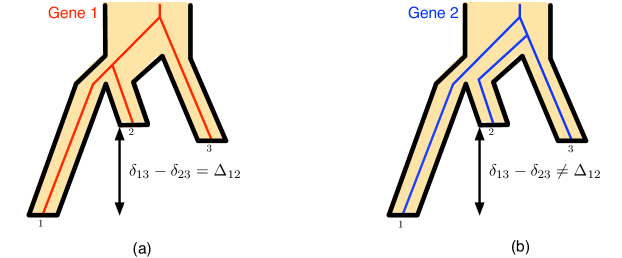
Figure 3: (a) Gene 1 (red gene) has the topology $12|3$. Therefore, the gene distance on this gene satisfies the condition that $\delta_{13}-\delta_{23}=\Delta_{12}$. (b) In this case, Gene 2 (blue gene) has the topology $1|23$. Observe that therefore, $\delta_{13}-\delta_{23}\neq\Delta_{12}$.

More formally, we establish the following two propositions, whose proofs are in Section B. For $x,y\in L$ and $\beta\in[0,1]$, let $\delta_{xy}^{(\beta)}$ be the $\beta$-th quantile of $\delta_{xy}$. That is, $\delta_{xy}^{(\beta)}$ is the smallest number $\alpha\in[0,1]$ such that

$$\mathbb{P}\left[\delta_{xy}\leq\alpha\right]\geq\beta.$$

Note that this quantile is a function of the distribution of $G$ (and of the $\vec{\delta}$s). Our event of interest is defined next.

Proposition 1 (Fixing the rooted topology of the gene tree).

Let $(x,y,z)$ be an arbitrary permutation of $(1,2,3)$. The event

$$\mathscr{E}_{I}=\left\{\delta_{xy}\leq\delta_{xy}^{(1/2)},\delta_{xz}>\delta_{xz}^{(1/2)},\delta_{yz}>\delta_{yz}^{(1/2)}\right\},$$ (4)

has positive probability and implies that the rooted topology of $G$ is $xy|z$.

Conditioning on the event $\mathscr{E}_{I}$, we then show how to recover the difference $\Delta_{xy}$ from the distribution of $\delta_{xz}-\delta_{yz}$.

Proposition 2 (A formula for the height difference).

Using the notation of Proposition 1, we have

$$\mathbb{E}[\delta_{xz}-\delta_{yz}\,|\,\mathscr{E}_{I}]=\Delta_{xy},$$ (5)

almost surely.

Note that the quantity on the l.h.s. of (5) is a function of the distribution of $G$. From the values of $\Delta_{xy},x,y\in\mathcal{X}$, we can solve for $\mu_{rx},x\in\mathcal{X}$. Hence, combining the properties of the Farris transform with Propositions 1 and 2, we arrive at Theorem 3.

3.2 Algorithm 2: the reduction step

We are now ready to describe the reduction algorithm (Algorithm 2) and provide guarantees about its behavior. Recall that we are restricting our attention to three leaves $\mathcal{X}=\left\{1,2,3\right\}$ whose species tree topology is $12|3$. The main idea underlying the reduction algorithm is based on the proof of the identifiability result (Theorem 3). That is, we find a set of genes whose topology is highly likely to be a fixed triplet, we estimate the height differences on this set using the “sample version” of (5), and we perform what could be thought of as a “sequence-based” Farris transform.

Given that we do not have access to the actual gene tree distribution, but only sequence data, there are several differences with the identifiability proof that make the analysis and the algorithm more involved. A primary challenge is that, in the regime where sequence length is “short,” i.e., when $k\ll f^{-2}$, the sequence-based estimates of the gene tree distances are very inaccurate—much less accurate then what is needed for our reduction step to be useful.

Key idea 2: To get around this issue, we show how to combine genes satisfying a condition similar to (4) to produce a much better estimate of distance differences.

We detail the main steps of Algorithm 2 next.

Fixing gene tree topologies.

Here we only have access to sequence data. In particular the $\delta$s are unknown. So, we work instead with the $p$-distances

$$\widehat{p}_{xy}^{i}=\frac{1}{k}\sum_{j\in[k]}\mathbbm{1}\left\{\xi^{ij}_{x}\neq\xi^{ij}_{y}\right\},$$

for gene $i$ and $x,y\in\mathcal{X}$, and their empirical quantiles $\widehat{p}^{(\beta)}_{xy}$. Similar to Proposition 1, we then consider those genes for which the event

$$\left\{\widehat{p}_{xy}^{i}\leq\widehat{p}_{xy}^{(1/3)},\widehat{p}_{xz}^{(2/3)}\leq\widehat{p}_{xz}^{i}\leq\widehat{p}_{xz}^{(5/6)},\widehat{p}_{yz}^{(2/3)}\leq\widehat{p}_{yz}^{i}\leq\widehat{p}_{yz}^{(5/6)}\right\},$$ (6)

holds for some chosen permutation $(x,y,z)$ of $(1,2,3)$. We will call this set of genes $I$. We show that this set has a “non-trivial” size and that, with high probability, the genes satisfying (6) have topology $xy|z$ (see Proposition 5). In particular, the analysis of this construction accounts for the “sequence noise” around the expected values

$$p^{i}_{xy}\triangleq\mathbb{E}\left[\widehat{p}^{i}_{xy}\middle|G^{(i)}\right]=\frac{3}{4}\left(1-e^{-4\delta^{i}_{xy}/3}\right)\triangleq p(\delta^{i}_{xy}),$$ (7)

where $p(x)=\frac{3}{4}\left(1-e^{-4x/3}\right)$.

Estimating distance differences.

Because we work with $p$-distances, we adapt formula (5) for the difference $\Delta_{xy}$ as follows. Using

$$\widehat{p}^{I}_{xz}=\frac{1}{\left|I\right|}\sum_{i\in I}\widehat{p}_{xz}^{i}\qquad\text{and}\qquad\widehat{p}^{I}_{yz}=\frac{1}{\left|I\right|}\sum_{i\in I}\widehat{p}_{yz}^{i},$$

our estimate of the distance differences is given by

$$\widehat{\Delta}_{xy}=\left\{-\frac{3}{4}\log\left(1-\frac{4}{3}\widehat{p}_{xz}^{I}\right)\right\}-\left\{-\frac{3}{4}\log\left(1-\frac{4}{3}\widehat{p}_{yz}^{I}\right)\right\}.$$

Recall that, for this formula to work, we need to ensure that the topologies of the gene trees used are fixed to be $xy|z$; see Fig. 3, for instance. The logarithmic transforms in the curly brackets are the usual distance corrections in the Jukes-Cantor sequence model (see e.g. [Ste16]). Note, however, that we perform an average over $I$ before the correction; this is important to obtain the correct statistical power of our estimator. A similar phenomenon was leveraged in the METAL algorithm of [DNR15]. The non-trivial part of the analysis of this step is to bound the estimation error. Indeed, unlike the identifiability result, we have a finite amount of gene data and, moreover, we must account for the sequence noise. This is done using concentration inequalities in Proposition 6.

Stochastic Farris transform.

The quantile test of Section E below is not a distance-based method in the traditional sense of the term. That is, we do not define a pairwise distance matrix on the leaves and use it to deduce the species phylogeny. Instead, our method uses the empirical distribution of the $p$-distances across genes. It is for this reason that we do not simply apply the classical Farris transform of (3) to the estimated distances. Rather, we perform what we call a “stochastic” Farris transform. That is, we transform the sequence data itself to mimic the distribution under an ultrametric species phylogeny.

Key idea 3: This is done by adding the right amount of noise to the sequence data at each gene, as detailed next. It ensures that we properly mimic the contributions from both the multispecies coalescent and the Jukes-Cantor model to the distribution of $p$-distances.

See Algorithm 2 for the full details.

For the sake of notational convenience, we will let $\oplus$ denote addition mod-4 and identify ${\tt A,T,G,C}$ with $\{0,1,2,3\}$ in that order when doing this addition. For instance, this means that ${\tt A}\oplus 1={\tt T}$ and ${\tt G}\oplus 2={\tt A}$.

Definition 5 (Stochastic Farris transform).

For a gene $i$, let $\{\xi_{x}^{i}\}_{x\in\mathcal{X}}$ be a sequence dataset over the species $\mathcal{X}=\{1,2,3\}$ and let $\Delta_{xy}=\mu_{rx}-\mu_{ry},x,y\in\mathcal{X}$. Assume without loss of generality that $\min\{\Delta_{12},\Delta_{13}\}\geq 0$. The stochastic Farris transform defines a new set of sequences $\{\xi^{i}_{x,N}\}_{x\in\mathcal{X}}$ such that $\xi_{x,N}^{i}=\xi_{x}^{i}\oplus\epsilon_{x}^{i}$, where $\epsilon_{x}^{i}\in\{0,1,2,3\}^{k}$ is an independent random sequence whose $j$-th coordinate is drawn according to

$$\epsilon_{x}^{ij}=\begin{cases}0,&\mbox{ w.p. }1-p(\Delta_{1x}),\\ 1,&\mbox{ w.p. }p(\Delta_{1x})/3,\\ 2,&\mbox{ w.p. }p(\Delta_{1x})/3,\\ 3,&\mbox{ w.p. }p(\Delta_{1x})/3.\end{cases}$$

We write this as $\{\xi_{x,N}^{i}\}_{x\in\mathcal{X}}=\mathcal{F}(\{\xi_{x}^{i}\}_{x\in\mathcal{X}};\{\Delta_{xy}\}_{x,y\in\mathcal{X}})$.

By the Markov property, for $x,y\in\mathcal{X}$, the “noisy” sequence data above satisfy

$$\mathbb{P}\left[\xi_{x,N}^{i}\neq\xi_{y,N}^{i}\right] =p\left(\delta_{xy}^{i}+\Delta_{1x}+\Delta_{1y}\right)\triangleq r_{xy}^{i}.$$

Notice that $\delta_{xy}^{i}$, the random gene tree distance between $x$ and $y$ under gene $i$, can be decomposed as $\mu_{xy}+\Gamma_{xy}^{i}$, where $\Gamma_{xy}^{i}$ is the random component contributed by the multispecies coalescent. On the other hand, the set of distances $\mu_{xy}+\Delta_{1x}+\Delta_{1y}$ is ultrametric by the properties of the classical Farris transform. As a result, the stochastic Farris transform modifies the sequence data so that it appears as though it was generated from an ultrametric MSC-JC process. We show this pictorially in Fig. 4.

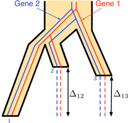
Figure 4: After the stochastic Farris transform, the leaf edges corresponding to leaves $2$ and $3$, in both Gene 1 (red gene) and Gene 2 (blue gene), are “stretched” by $\Delta_{12}$ and $\Delta_{13}$ respectively. As a result, the sequence data appears as though it is drawn from an ultrametric species phylogeny.

In reality, we do not have access to the true differences $\Delta_{xy},x,y\in\mathcal{X}$. Instead, we employ our estimates $\widehat{\Delta}_{xy}$ for all $x,y\in\mathcal{X}$ in the previous step to obtain the following approximate stochastic Farris transform:

$$\{\xi_{x,N}^{i}\}_{x\in\mathcal{X}}=\mathcal{F}(\{\xi_{x}^{i}\}_{x\in\mathcal{X}};\{\widehat{\Delta}_{xy}\}_{x,y\in\mathcal{X}}).$$ (8)

This is the output of the reduction. See Algorithm 2 for details. We prove Theorem 2 in Section D. In what follows, we will condition on the implications of Theorem 2 holding.

4 Concluding remarks

We have extended the optimal tradeoff (up to log factors) of [MR15] beyond the case of equal mutation rates and population sizes. Several open problems remain:

1. Our results assume that the number of leaves $n$ is constant (as $k,m\to\infty$). As $n$ gets larger, the depth of the species phylogeny typically increases. In fact, in the single gene tree reconstruction context, the depth is known to play a critical and intricate role in the data requirement [ESSW99a, Mos04, Mos07, DMR11a, DMR11b]. Understanding the role of the depth under the MSC-JC is an interesting avenue for future work.

2. We have assumed here that the mutation rates are the same across genes. This assumption is not realistic and relaxing it is important for the practical relevance of this line of work. Identifiability issues may arise however [MS07, Ste09]. In a related issue, we have assumed, to simplify, that all genes have the same length. (Gene lengths and mutation rates together control the amount of phylogenetic signal in a gene.) We leave for future work how best to take advantage of differing gene lengths (beyond simply truncating to the shortest gene).

3. A more technical point left open here is to remove the assumption that $k$ grows polynomially with $f$. This may require new ideas.

Appendix A Models: full definitions

In this section, we provide full definitions of the multispecies coalescent and Jukes-Cantor model.

Jukes-Cantor model of sequence evolution

The Jukes-Cantor model of sequence evolution is detailed in Algorithm 3.

1. Associate to the root $r$ a sequence $\xi_{r}=\left\{\xi_{r}^{1},\ldots,\xi_{r}^{k}\right\}\in\left\{{\tt A,T,G,C}\right\}^{k}$ of length $k$, where each character $\xi_{r}^{j}$ is drawn independently and uniformly at random from $\left\{{\tt A,T,G,C}\right\}$.

2. Initialize the set $U$ with the children of the root $r$ of $G^{(i)}$.

3. Repeat until $U=\emptyset$.

   1. Pick $u\in U$, and let $u^{-}$ be the parent of $u$ in $G^{(i)}$.

   2. Associate a sequence $\xi_{u}\in\left\{{\tt A,T,G,C}\right\}^{k}$ as follows. $\xi_{u}$ is obtained from $\xi_{u^{-}}$ by mutating each site independently with probability $p_{(u,u^{-})}$. If a mutation occurs at a site $j$, it gets assigned a uniformly random character from $\left\{{\tt A,T,G,C}\right\}$, else the corresponding character from $\xi_{u^{-}}$ simply gets copied.

   3. Remove $u$ from $U$ and add any children of $u$ to $U$.

Algorithm 3: The Jukes-Cantor process

Multispecies coalescent

Function MSC($v_{\rm c}{}$).

1. If $v_{\rm c}{}\in L$, i.e., $v_{\rm c}$ is a leaf of $S$:

   1. Return the following single edge (root-extended) tree: $(v_{\rm c}{},r^{\prime})$. One vertex of this edge corresponds to the current leaf and the other is an ancestor to this leaf, and the root of the tree. The length of the edge created is $\mu_{e}\times\tau_{e}$, where $e\in E_{s}$ is the edge incident upon $v_{\rm c}{}$ in $S$.

2. Else

   1. Let $d_{1}$ and $d_{2}$ be the descendants of $v_{\rm c}{}$.

   2. If $v_{\rm c}{}$ is $r$, the root of $S$, then set $\tau,\mu=\infty$. Otherwise, let $\tau$ and $\mu$ respectively be the length and mutation rate of the branch connecting $v_{\rm c}{}$ to its immediate ancestor in $S$.

   3. Return the following forest: coalesce(MSC($d_{1}$), MSC($d_{2}$), $\tau$, $\mu$)

Function coalesce($F_{1}$, $F_{2}$, $\tau$, $\mu$).

1. Create a new forest $F$ that is a union of $F_{1}$ and $F_{2}$. Set $k=$ number of roots (or lineages) in $F$.

2. While $k>1$:

   1. Choose a random pair of (distinct) roots $r_{1}$ and $r_{2}$ from $F$. Also draw a random time $t\sim$ Exp$({k\choose 2})$.

   2. If $t\geq\tau$

      1. Increase the length of all the $k$ root edges in $F$ by $\mu\times\tau$. Return $F$.

   3. Else

      1. Set $\tau:=\tau-t$. Create new vertices $r_{3},r_{3}^{\prime}$.

      2. Make $r_{1}$ and $r_{2}$ descendants of $r_{3}$, where the lengths of the branches ($r_{1}$ , $r_{3}$) and ($r_{2}$, $r_{3}$) are both set equal to $\mu\times t$. Make $r_{3}^{\prime}$ the root of this newly created tree, connecting $r_{3}^{\prime}$ to $r_{3}$ with a length $0$ branch.

      3. Also, add $\mu\times t$ to the root edges of the other trees in $F$. Now, $F$ has one fewer root, so set $k:=k-1$.

3. If $k$ is 1, then return $F$, adding $\mu\times\tau$ to the unique root edge of $F$.

Algorithm 4: The multispecies coalescent process

Let $S=(V_{s},E_{s};r,\vec{\tau},\vec{\mu})$ be a fixed species phylogeny. For the sake of this algorithmic description, we will work with what we call root-extended trees and forests. Given a weighted rooted tree, the corresponding root-extended tree simply has a new vertex $r^{\prime}$ that is connected to $r$ with a (potentially zero-) weighted edge. We will call $r^{\prime}$ the root of such a tree, and the edge connecting $r$ and $r^{\prime}$ as the root edge. A root-extended forest is simply a union of root-extended trees. Only for the description that follows, when we write tree and forest, we mean the root-extended versions unless otherwise specified.

We first describe a function MSC that takes as input a vertex $v_{\rm c}{}\in V_{s}$, and returns a forest. We will obtain a random gene tree from the multispecies coalescent as follows: (1) invoke the function MSC with $r$, the root of $S$ as input, and (2) contract the root-edge of the tree returned (thus making it a gene tree per Definition 2). That is, for $i\in[m]$, $G^{(i)}=$ MSC$(r)$, with the root edge contracted. This function, as we can see in Algorithm 4, recursively descends the species phylogeny $S$ and it calls the function coalesce() at every stage of this recursion.

The coalesce() function works with rooted forests. This function operates at each branch of the species tree, and (potentially) merges the genealogies of its two descendant populations. It takes as input two forests $F_{1}$ and $F_{2}$ corresponding to the descendants of the current branch (or population) that it is invoked at. It also takes the mutation rate $\mu$ and length $\tau$ associated with the current branch. It then returns a single forest $F$ after performing (potentially) multiple coalescence operations. The details are in Algorithm 4.

Fig. 2 shows two sample draws from the multispecies coalescent process. Notice that while the topology of Gene 1 (red gene) agrees with the topology of the underlying species tree, the topology of Gene 2 (blue gene) does not. This happens since in Step 2(b) of coalesce, if the randomly drawn time $t$ is larger than $\tau$, the chosen pair of lineages do not coalesce in the current population. This sort of discordance in the topologies of gene trees is called incomplete lineage sorting (ILS). For more details, we refer the reader e.g. to [DR09].

The density of the likelihood of a gene tree ${G}^{(i)}=\left({V}^{(i)},{E}^{(i)}\right)$ can now be written down as follows. We will focus our attention on the branch $e\in E$ of the species tree and for the gene tree $G^{(i)}$, let $I^{(i)}_{e}$ and $O^{(i)}_{e}$ be the number of lineages entering and leaving the branch $e$ respectively. For instance, consider Gene 1 in Figure 5.

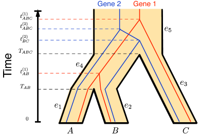
Figure 5: A species phylogeny (the thick, shaded tree) and two samples from the multispecies coalescent.

Here, two lineages enter the branch $e_{4}$ and one lineage leaves it. On the other hand, in the case of Gene 2 in Figure 5, two lineages enter the branch $e_{4}$ and two lineages leave it. Let $t_{e,s}^{(i)},s=\left\{1,2,\ldots,I_{e}^{(i)}-O_{e}^{(i)}+1\right\}$ be the $s-$th coalescent time corresponding to $G^{(i)}$ in the branch $e$. From the algorithm described above, each pair of lineages in a population can coalesce at a random time drawn according to the Exp$(1)$ distribution independently of each other. Therefore, after the $(s-1)$-th coalescent event at time $t_{e,s-1}^{(i)}$, there are $I_{e}^{(i)}-s+1$ surviving lineages in branch $e$ and the likelihood that the $s-$th coalescence time in branch $e$ is $t_{e,s}^{(i)}$ corresponds to the event that the minimum of ${I_{e}^{(i)}-s+1\choose 2}$ random variables distributed according to Exp$(1)$ has the value $t_{e,s}^{(i)}-t_{e,s-1}^{(i)}$. It follows that the density of the likelihood of $G^{(i)}$ can be written as

$$\prod_{e\in E}\prod_{s=1}^{I^{(i)}_{e}-O_{e}^{(i)}+1}\exp\left\{-{I_{e}^{(i)}-s+1\choose 2}\left[t_{e,s}^{(i)}-t_{e,s-1}^{(i)}\right]\right\},$$ (9)

where, for convenience, we let $t^{(i)}_{e,0}$ and $t^{(i)}_{e,I^{(i)}_{e}-O^{(i)}_{e}+1}$ be respectively the divergence times of the population in $e$ and of its parent population.

We will also need the density and quantiles of gene tree pairwise distances. For a pair of leaves $a,b\in L$, $\delta_{ab}$ is the branch length induced by the random gene tree which is drawn according to the MSC. Notice that, by definition, $\delta_{ab}\geq\mu_{ab}$ . We will let $f_{ab}\left(\cdot\right)$ and $F_{ab}\left(\cdot\right)$ denote respectively the density and the cumulative density function of the random variable $Z_{ab}\triangleq\frac{\delta_{ab}-\mu_{ab}}{2}$. Because of the memoryless property of the exponential, it is natural to think of the distribution of $Z_{ab}$ as a mixture of distributions whose supports are disjoint, corresponding to the different branches that the lineages go through before coalescing. We state this more generally as follows. Suppose that $U_{1},U_{2},\ldots,U_{r}$ are subsets of $\mathbb{R}$ such that they satisfy

$$\sup(U_{i})\leq\inf(U_{i+1}),\;\;\;i=1,2,\ldots,r.$$

Suppose that $f$ is a probability density function such that

$$f(x)=\sum_{i=1}^{r}\omega_{i}f_{i}(x),$$

where $\omega_{1},\omega_{2},\ldots,\omega_{r}\in(0,1)$ are such that $\sum_{i=1}^{r}\omega_{i}=1$, and the density $f_{i}$ is supported on $S_{i}$ for $i=1,\ldots,r$. Then, the quantile function of $f$ is given as follows

$$\mathbb{Q}_{F}(\alpha)\triangleq\inf\left\{x\in\mathbb{R}:\alpha\leq F(x)\right\}=\sum_{i=1}^{r}\mathbbm{1}\left\{\alpha\in\left[\sum_{j=0}^{i-1}\omega_{j},\sum_{j=0}^{i}\omega_{j}\right)\right\}\mathbb{Q}_{F_{i}}\left(\frac{\alpha-\sum_{j=0}^{i-1}\omega_{i}}{\omega_{i}}\right),$$

where, we set $\omega_{0}=0$. Specializing to $f_{ab}$ under the multispecies coalescent, it follows that there exists a finite sequence of constants $\mu_{1},\ldots,\mu_{r}\in[\mu_{L},\mu_{U}]$ and $h_{0},\ldots,h_{r-1}\in[f^{\prime},g^{\prime}+ng]$ such that

$$\omega_{i}=e^{-\sum_{j=1}^{i-1}\mu_{j}^{-1}(h_{j}-h_{j-1})}-e^{-\sum_{j=1}^{i}\mu_{j}^{-1}(h_{j}-h_{j-1})},$$

and

$$f_{i}(x)=\frac{\mu_{i}^{-1}e^{-\mu_{i}^{-1}(x-h_{i-1})}}{1-e^{-\mu_{i}^{-1}(h_{i}-h_{i-1})}}.$$

Cancellations lead to

$$f_{ab}(x)=\sum_{i=1}^{r}e^{-\sum_{j=1}^{i-1}\mu_{j}^{-1}(h_{j}-h_{j-1})}\mu_{i}^{-1}e^{-\mu_{i}^{-1}(x-h_{i-1})}.$$

This formula implies that the density is bounded between positive constants. We will need the following implication. For any $\alpha\in[0,1)$, we let $\delta_{ab}^{(\alpha)}$ and $p_{ab}^{(\alpha)}$ denote the $\alpha$-quantile of the $\delta_{ab}$ and $p_{ab}$ respectively. Since by definition $p_{ab}=p(\delta_{ab})$, we have that $p^{(\alpha)}_{ab}=p(\delta_{ab}^{(\alpha)})$, where $p(x)=\frac{3}{4}\left(1-e^{-4x/3}\right)$. Then, for any $0<\beta^{\prime}<\beta<1$, there are constants $0<c^{\prime}<c^{\prime\prime}<+\infty$ (depending on $\mu_{L},\mu_{U},g,g^{\prime},n,\beta^{\prime},\beta$) such that for any $\xi\in(0,1-\beta^{\prime})$, we have

$$c^{\prime}\xi\leq\delta_{ab}^{(\beta+\xi)}-\delta_{ab}^{(\beta)}\leq c^{\prime\prime}\xi,$$ (10)

and, hence,

$$c^{\prime}\xi\leq p_{ab}^{(\beta+\xi)}-p_{ab}^{(\beta)}\leq c^{\prime\prime}\xi.$$ (11)

Appendix B Identifiability result: proofs

The key steps in the proof of Theorem 3 follow.

Proof (Proposition 1): Recall the definition of the event

$$\mathscr{E}_{I}=\left\{\delta_{xy}\leq\delta_{xy}^{(1/2)},\delta_{xz}>\delta_{xz}^{(1/2)},\delta_{yz}>\delta_{yz}^{(1/2)}\right\}.$$

Our goal is to show that it has positive probability and that it implies that the rooted topology of $G$ is $xy|z$. This makes sense on an intuitive level because the event $\mathscr{E}_{I}$ requires that $\delta_{xy}$ is somewhat small and that $\delta_{xz}$, $\delta_{yz}$ are somewhat large. To make this rigorous we use the fact that, conditioned on coalescence occurring in the top population, the time to coalescence inside that population is identically distributed for all pairs of lineages. That observation facilitates the comparison the $\delta$-quantiles, as we show now.

Let $\Gamma_{xy}$ be twice the weighted height of the MSC process between the lineages of $x$ and $y$ in the common ancestral population. Notice that with this definition of $\Gamma_{xy}$, we can write $\delta_{xy}=\mu_{xy}+\Gamma_{xy}$. We let $\Gamma_{xy}=0$ if the coalescence between the lineages of $x$ and $y$ occurs below the common ancestral population (which in this case is only possible for the two closest populations in the species tree), an event we denote by $\mathscr{B}_{xy}$. For $\beta\in[0,1]$, let $\Gamma_{xy}^{(\beta)}$ be the $\beta$-th quantile of $\Gamma_{xy}$. We define the quantities above similary for the other pairs. We make three observations:

1. By definition of $\Gamma_{xy}$, the event $\{\delta_{xy}\leq\delta_{xy}^{(1/2)}\}$ implies the event $\{\Gamma_{xy}\leq\Gamma_{xy}^{(1/2)}\}$. (Note that the two events are not in fact equivalent, though, because of the possibility that $\Gamma_{xy}^{(1/2)}=0$.) Similarly, $\{\delta_{xz}>\delta_{xz}^{(1/2)}\}$ implies $\{\Gamma_{xz}>\Gamma_{xz}^{(1/2)}\}$ and $\{\delta_{yz}>\delta_{yz}^{(1/2)}\}$ implies $\{\Gamma_{yz}>\Gamma_{yz}^{(1/2)}\}$.

2. Irrespective of the species tree topology, the lineages of at least of one the pairs $(x,z)$ or $(y,z)$ can only coalesce in the common ancestral population. See Figures 2 and 3, for instance.

3. By symmetry, conditioned on coalescence in the common ancestral population, all $\Gamma$s are equal in distribution, i.e.,

   $$\Gamma_{xy}\,|\,\mathscr{B}_{xy}^{c}\stackrel{{\scriptstyle\rm d}}{{=}}\Gamma_{xz}\,|\,\mathscr{B}_{xz}^{c}\stackrel{{\scriptstyle\rm d}}{{=}}\Gamma_{yz}\,|\,\mathscr{B}_{yz}^{c}.$$

As a consequence of b) and c), we have

$$\Gamma_{xy}^{(1/2)}\leq\max\{\Gamma_{xz}^{(1/2)},\Gamma_{yz}^{(1/2)}\},$$ (12)

where we used that, conditioned on $\mathscr{B}_{xy}$, it holds that $\Gamma_{xy}=0$. Combining this with a), we get that $\mathscr{E}_{I}$ implies the event

$$\left\{\Gamma_{xy}\leq\Gamma_{xy}^{(1/2)},\Gamma_{xz}>\Gamma_{xz}^{(1/2)},\Gamma_{yz}>\Gamma_{yz}^{(1/2)}\right\},$$

which together with (12) implies the event

$$\Gamma_{xy}<\max\{\Gamma_{xz},\Gamma_{yz}\}.$$

This last event can only happen when the gene tree topology is $xy|z$.

It remains to prove that $\mathscr{E}_{I}$ has positive probability. Let $\mathscr{F}$ be the event that $G$ has rooted topology $xy|z$. Note that

$$\mathbb{P}[\mathscr{E}_{I}] \geq \mathbb{P}[\mathscr{E}_{I},\mathscr{F}]$$

$$= \mathbb{P}[\delta_{xy}\leq\delta_{xy}^{(1/2)}]\,\mathbb{P}[\mathscr{F}\,|\,\delta_{xy}\leq\delta_{xy}^{(1/2)}]\,\mathbb{P}[\delta_{xz}>\delta_{xz}^{(1/2)},\delta_{yz}>\delta_{yz}^{(1/2)}\,|\,\mathscr{F},\delta_{xy}\leq\delta_{xy}^{(1/2)}],$$

where each term on the last line is clearly positive under the MSC. $\blacksquare$

Proof (Proposition 2): Conditioned on $\mathscr{E}_{I}$, we know from Lemma 1 that the coalescence between the lineages of $x$ and $z$ happens in the common ancestral population of $x,y$ and $z$, irrespective of the species tree topology. The same holds for $y$ and $z$. This implies that

$$\delta_{xz}=\mu_{rx}+\mu_{rz}+\Gamma_{xz},$$ (13)

and

$$\delta_{yz}=\mu_{ry}+\mu_{rz}+\Gamma_{yz},$$ (14)

where the $\Gamma$s are defined in the proof of Lemma 1. Observe further that in fact, conditioned on $\mathscr{E}_{I}$,

$$\Gamma_{xz}=\Gamma_{yz},$$ (15)

almost surely. Hence, combining (13), (14), and (15),

$$\mathbb{E}[\delta_{xz}-\delta_{yz}\,|\,\mathscr{E}_{I}]=\mu_{rx}-\mu_{ry}=\Delta_{xy},$$

as claimed. $\blacksquare$

Appendix C Main theorem: proof

Theorem 1 follows from Proposition 3 below.

Proposition 3 (Data requirement: general version).

Suppose we have data $\left\{\xi^{ij}\right\}_{i\in[m],j\in[k]}$ generated according to the MSC-JC$(m,k)$ process on a species phylogeny $S=(V_{s},E_{s};r,\vec{\tau},\vec{\mu})$. The mutation rates, leaf-edge lengths and internal-edge lengths are respectively in $(\mu_{L},\mu_{U})$, $(f^{\prime},g^{\prime})$ and $(f,g)$. For any $\varepsilon>0$ and $C>0$ there is a constant $c_{1}>0$ such that Algorithm 1 correctly identifies the topology of $S$ restricted to $\mathcal{X}=\{1,2,3\}$ with probability at least $1-\varepsilon$, provided there is a partitioning of the set of genes $[m]=\mathcal{M}_{{\rm R}1}\sqcup\mathcal{M}_{{\rm R}2}\sqcup\mathcal{M}_{{\rm Q}1}\sqcup\mathcal{M}_{{\rm Q}2}$ such that the following conditions hold:

$$\left|\mathcal{M}_{{\rm R}1}\right| \geq c_{1}\log\varepsilon^{-1}\phantom{\left(c_{2}\frac{\log k}{kf^{2}}\right)}$$

$$\left|\mathcal{M}_{{\rm Q}1}\right| \geq c_{1}\alpha^{-1}\log\varepsilon^{-1}$$

$$\begin{aligned} \left|\mathcal{M}_{{\rm R}2}\right|&\geq c_{1}\left(1\vee\frac{\log k}{kf^{2}}\right)\log\varepsilon^{-1}\\ \left|\mathcal{M}_{{\rm Q}2}\right|&\geq c_{1}f^{-2}\left(\alpha+f\right)\log\varepsilon^{-1},\end{aligned}$$

where $\alpha=m^{-1}\log m\vee k^{-0.5}\sqrt{\log k}$. And, the sequence length $k$ satisfies:

$$k \geq c_{1}\log\left(\left|\mathcal{M}_{{\rm R}2}\right|\varepsilon^{-1}\right)\vee c_{1}\left(f^{-1}\sqrt{\log k}\right)^{C}.$$

Under condition (1) of Theorem 1, to satisfy the inequalities above, we can choose $|\mathcal{M}_{{\rm R}1}|\gtrsim 1$, $|\mathcal{M}_{{\rm R}2}|\gtrsim 1\lor\frac{1}{kf^{2}}$, $|\mathcal{M}_{{\rm Q}1}|\gtrsim 1$ and $|\mathcal{M}_{{\rm Q}2}|\gtrsim\frac{1}{f}\lor\frac{1}{\sqrt{k}f^{2}}$.

Proof (Proposition 3): Without loss of generality we assume that the topology of the true species tree restricted to this triple is $12|3$.

Main steps

Let $S_{\mathcal{X}}$ be the species tree $S$ restricted to $\mathcal{X}=\{1,2,3\}$ and let $r^{\prime}$ denote its root, i.e., the most recent common ancestor of $\mathcal{X}$. We let $\alpha=\max\left\{m^{-1}\log m,k^{-0.5}\sqrt{\log k}\right\}$. We partition the loci $[m]=\mathcal{M}_{{\rm R}1}\sqcup\mathcal{M}_{{\rm R}2}\sqcup\mathcal{M}_{{\rm Q}1}\sqcup\mathcal{M}_{{\rm Q}2}$, such that the size of each partition satisfies the conditions specified in Proposition 3. The reconstruction algorithm on $\mathcal{X}$ has two steps: 1) a reduction to the ultrametric case by the addition of noise and 2) the ultrametric quantile test. We divide the proof accordingly:

1. Ultrametric reduction: In this step, we invoke Algorithm 2 with sequence data $\{\xi_{x}^{ij}:x\in\mathcal{X},i\in[m],j\in[k]\}$. The algorithm outputs new sequences $\{\xi_{x,N}^{ij}:x\in\mathcal{X},i\in\mathcal{M}_{{\rm Q}1}\sqcup\mathcal{M}_{{\rm Q}2},j\in[k]\}$, and Proposition 4 (proved in Section D) guarantees that these output sequences appear as though they were drawn from an almost-ultrametric species phylogeny $S_{\mathcal{X}}^{\prime}$ that has the same topology as $\mathcal{S}_{\mathcal{X}}$. In particular, using Proposition 4, we know that there is a constant $c_{1}>0$ such that if

   $$|\mathcal{M}_{{\rm R}1}|,|\mathcal{M}_{{\rm R}2}|\geq c_{1}\log(4\varepsilon^{-1}),$$

   $$k\geq c_{1}\log|\mathcal{M}_{{\rm R}2}|+c_{1}\log(4\varepsilon^{-1}),$$

   $$k|\mathcal{M}_{{\rm R}2}|\geq c_{1}\phi^{-2}\log(4\varepsilon^{-1}).$$

   then, $\{\xi^{ij}_{x,N}:x\in\mathcal{X},i\in\mathcal{M}_{{\rm Q}1}\sqcup\mathcal{M}_{{\rm Q}2},j\in[k]\}$ has the same distribution as a multispecies coalescent process on $S_{\mathcal{X}}^{\prime}$ with branch lengths $(\hat{\dot{\mu}}_{xy})$, where $S_{\mathcal{X}}^{\prime}$ and $S$ have the same rooted topology, and $(\hat{\dot{\mu}}_{xy})$ and $({\dot{\mu}}_{xy})$ are $\mathcal{O}(f/\sqrt{\log k})$-close with probability at least $1-\varepsilon$. Notice that we have set the value of $\phi$ in Proposition 4 to $\mathcal{O}(f/\sqrt{\log k})$, which will turn out to be what we need in Step 2 below.

2. Quantile test: Now, we invoke Algorithm 1 with the sequence data $\{\xi_{x,N}^{ij}:i\in\mathcal{M}_{{\rm Q}1}\sqcup\mathcal{M}_{{\rm Q}2},j\in[k]\}$ output by Step 1. By Propositions 7 and 9 (proved in Section E), it follows that if

   $$\left|\mathcal{M}_{{\rm Q}1}\right| \geq c_{1}\alpha^{-1}\log\varepsilon^{-1}$$

   $$\left|\mathcal{M}_{{\rm Q}2}\right| \geq c_{1}f^{-2}\left(\alpha+f\right)\log\varepsilon^{-1},$$

   then, with probability at least $1-\varepsilon$, Algorithm 1 returns the right topology .

This concludes the proof. $\blacksquare$

Appendix D Ultrametric reduction: proofs

Theorem 2 follows from Proposition 4 below. In Proposition 4, we show that the approximate stochastic Farris transform defined in Section 3.2 outputs sequence data that looks statistically as though it was generated from an ultrametric species phylogeny.

Given estimates $\widehat{\Delta}_{xy}$ for all $x,y\in\mathcal{X}$, and supposing that $\min\{\widehat{\Delta}_{12},\widehat{\Delta}_{13}\}\geq 0$ (the other cases follow similarly), we let

$$\widehat{\dot{\mu}}_{xy}=\mu_{xy}+\widehat{\Delta}_{1x}+\widehat{\Delta}_{1y},\qquad x,y\in\mathcal{X}.$$

Compare this to the definition of $\dot{\mu}_{xy}$ in (3). Recall Definition 1, and let $S^{\prime}=(V_{s},E_{s},r,\vec{\tau},\vec{\hat{\dot{\mu}}})$ be a species phylogeny with the same topology and branch lengths as $S$ restricted to $\mathcal{X}$, and mutation rates $\{\widehat{\dot{\mu}}\}_{e\in E_{s}}$ that are chosen such that: (a) $\widehat{\dot{\mu}}_{e}=\mu_{e}$ if $e\in E_{s}$ is an internal branch, and (b) for all $e\in E_{s}$ that are incident on the leaves of $S$, let $\widehat{\dot{\mu}}_{e}$ be chosen (uniquely) such that mutation rate weighted distance on $S^{\prime}$ between any pair of leaves $x,y\in\mathcal{X}$ is given by $\widehat{\dot{\mu}}_{xy}$. The sets $\mathcal{M}_{{\rm R}1},\mathcal{M}_{{\rm R}2}$ referred to below are defined in Algorithm 2.

Proposition 4 (Ultrametric reduction: general version).

Suppose that we have sequence data $\left\{\xi^{ij}\right\}_{i\in[m],j\in[k]}$ generated according to the MSC-JC$(m,k)$ process on a three-species phylogeny $S=(V_{s},E_{s};r,\vec{\tau},\vec{\mu})$. The mutation rates, leaf-edge lengths and internal-edge lengths are respectively in $(\mu_{L},\mu_{U})$, $(f^{\prime},g^{\prime})$ and $(f,g)$. Then, the output of Algorithm 2 is distributed according to the MSC-JC process on the species tree $S^{\prime}$ defined above. Furthermore there is a constant $c_{2}>0$ such that, for any $\varepsilon,\phi\in(0,1)$, with probability at least $1-\varepsilon$, $\widehat{\dot{\mu}}_{xy}$ is $\phi$-close to the ultrametric $(\dot{\mu}_{xy})$, provided

$$|\mathcal{M}_{{\rm R}1}|,|\mathcal{M}_{{\rm R}2}|\geq c_{2}\log(4\varepsilon^{-1}),$$

$$k\geq c_{2}\log|\mathcal{M}_{{\rm R}2}|+c_{2}\log(4\varepsilon^{-1}),$$

$$k|\mathcal{M}_{{\rm R}2}|\geq c_{2}\phi^{-2}\log(4\varepsilon^{-1}).$$

Under condition (2) of Theorem 2, to satisfy the inequalities above, we can choose $|\mathcal{M}_{{\rm R}1}|\gtrsim 1$ and $|\mathcal{M}_{{\rm R}2}|\gtrsim 1\lor\frac{1}{kf^{2}}$.

D.1 Proof of Proposition 4

Proof (Proposition 4): As explained in Section 3.2, there are three main steps to this proof, which we summarize in a series of propositions.

For a gene $i$ and leaves $x,y\in\mathcal{X}$, let

$$\widehat{p}_{xy}^{i}=\frac{1}{k}\sum_{j\in[k]}\mathbbm{1}\left\{\xi^{ij}_{x}\neq\xi^{ij}_{y}\right\}.$$

Furthermore, we need to split the above average into two halves to avoid unwanted correlations as we explain below. We denote these as

$$\widehat{p}^{i\downarrow}_{xy}=\frac{2}{k}\sum_{j=1}^{k/2}\mathbbm{1}\{\xi^{ij}_{x}\neq\xi^{ij}_{y}\}\qquad\mbox{ and}\qquad\widehat{p}^{i\downarrow}_{xy}=\frac{2}{k}\sum_{j=k/2+1}^{k}\mathbbm{1}\{\xi^{ij}_{x}\neq\xi^{ij}_{y}\}.$$

And, for $\beta\in[0,1]$, let $\widehat{p}^{(\beta)}_{xy}$ be the corresponding empirical quantiles computed based on the set $\{\widehat{q}_{xy}^{i}:i\in\mathcal{M}_{{\rm R}1}\}$. Fix a permutation $(x,y,z)$ of $(1,2,3)$. Consider the following subset of genes in $\mathcal{M}_{{\rm R}2}$:

$$I=\left\{i\in\mathcal{M}_{{\rm R}2}\,:\,\widehat{p}^{i\downarrow}_{xy}\leq\widehat{p}_{xy}^{(1/3)},\widehat{p}_{xz}^{(2/3)}\leq\widehat{p}^{i\downarrow}_{xz}\leq\widehat{p}_{xz}^{(5/6)},\widehat{p}_{yz}^{(2/3)}\leq\widehat{p}^{i\downarrow}_{yz}\leq\widehat{p}_{yz}^{(5/6)}\right\}.$$

We first show that the rooted topologies in $I$ are highly likely to be $xy|z$. We also prove some technical claims that will be useful in the proof of Proposition 6 below.

Proposition 5 (Fixing gene tree topologies).

There are constants $c_{9},c_{10},c_{10}^{\prime},\varepsilon_{0}>0$ such that, with probability at least

$$1-10\exp(-2c_{9}^{2}|\mathcal{M}_{{\rm R}1}|)-6|\mathcal{M}_{{\rm R}2}|\exp\left(-k\varepsilon_{0}^{2}\right)-2\exp\left(-2c_{10}^{2}|\mathcal{M}_{{\rm R}2}|\right),$$

the following hold:

1. the rooted topology of all gene trees in $I$ is $xy|z$,

2. for all $i\in I$, $p^{i}_{xy}\leq p^{(7/24)}_{xy}$, $p^{(17/24)}_{xz}\leq p^{i}_{xz}\leq p^{(19/24)}_{xz}$, $p^{(17/24)}_{yz}\leq p^{i}_{yz}\leq p^{(19/24)}_{yz}$,

3. the size of $I$ is greater than $c_{10}^{\prime}|\mathcal{M}_{{\rm R}2}|$.

The proof is given in Section D.1.1. Notice that Proposition 5 guarantees that all the genes in $I$ satisfy conditions (a) and (b). We can weaken our requirements on how big $k$ needs to be by relaxing this and performing a more careful analysis.

Using

$$\widehat{p}^{I}_{xz}=\frac{1}{\left|I\right|}\sum_{i\in I}\widehat{p}_{xz}^{i\uparrow}\qquad\text{and}\qquad\widehat{p}^{I}_{yz}=\frac{1}{\left|I\right|}\sum_{i\in I}\widehat{p}_{yz}^{i\uparrow},$$

let

$$\widehat{\Delta}_{xy}=\left\{-\frac{3}{4}\log\left(1-\frac{4}{3}\widehat{p}_{yz}^{I}\right)\right\}-\left\{-\frac{3}{4}\log\left(1-\frac{4}{3}\widehat{p}_{xz}^{I}\right)\right\}.$$

Recall that

$$\Delta_{xy}=\mu_{rx}-\mu_{ry}.$$

We next show that $\widehat{\Delta}_{xy}$ is a good approximation to $\Delta_{xy}$. Let $\mathscr{I}$ be the event that the conclusion of Proposition 5 holds. To simplify the notation, throughout this proof, we use $\widetilde{\mathbb{P}}$ and $\widetilde{\mathbb{E}}$ to denote the probability and expectation operators conditioned on $\mathscr{I}$.

Proposition 6 (Estimating distance differences).

There is a constant $c_{11}\in(0,1)$ such that with $\widetilde{\mathbb{P}}$-probability at least

$$1-4\exp\left(-c_{11}k|\mathcal{M}_{{\rm R}2}|\phi^{2}\right),$$

the following holds:

$$\left|\widehat{\Delta}_{xy}-\Delta_{xy}\right|\leq\phi/2.$$

The proof is in Section D.1.2.

We repeat the height difference estimation above for all pairs in $\mathcal{X}$. Therefore, by a union bound, we get the above guarantee for all pairs with probability at least $1-12\exp\left(-c_{11}k|\mathcal{M}_{{\rm R}2}|\phi^{2}\right)$. Without loss of generality, assume that

$$\mu_{r1}\geq\max\{\mu_{r2},\mu_{r3}\},$$

and recall the Farris transform

$$\dot{\mu}_{xy}=\mu_{xy}+2\mu_{r1}-\mu_{rx}-\mu_{ry}=\mu_{xy}+\Delta_{1x}+\Delta_{1y},\qquad x,y\in\mathcal{X},$$

which defines an ultrametric, and consider the approximation

$$\widehat{\dot{\mu}}_{xy}=\mu_{xy}+\widehat{\Delta}_{1x}+\widehat{\Delta}_{1y},\qquad x,y\in\mathcal{X}.$$

Assuming that the conclusion of Proposition 6 holds for all $x,y\in\mathcal{X}$, we have shown that $(\widehat{\dot{\mu}}_{xy})$ is $\phi$-close to the ultrametric $(\dot{\mu}_{xy})$. As we explained in Section 3.2, we produce a new sequence dataset using an approximate stochastic Farris transform

$$\{\xi_{x,N}^{i}\}=\mathcal{F}(\{\xi_{x}^{i}\};(\widehat{\mu}_{rx})).$$

By the Markov property, the transformation $\mathcal{F}$ has the effect of stretching the leaf edges of the gene trees by the appropriate amount.

Hence, again by a union bound, we get the claim of Theorem 2 except with probability

$$10\exp(-2c_{9}^{2}|\mathcal{M}_{{\rm R}1}|)+6|\mathcal{M}_{{\rm R}2}|\exp\left(-2k\varepsilon_{0}^{2}\right)+2\exp\left(-2c_{10}^{2}|\mathcal{M}_{{\rm R}2}|\right)+12\exp\left(-c_{11}k|\mathcal{M}_{{\rm R}2}|\phi^{2}\right).$$ (16)

We can get the data requirement result by asking for the conditions under which the above quantity is less than $\varepsilon$. $\blacksquare$

D.1.1 Proof of Proposition 5

Proof (Proposition 5): Let $(x,y,z)$ be an arbitrary permutation of the leaves $(1,2,3)$. The idea of the proof is to rely on Proposition 1, which we rephrase in terms of $p$-distances. For a gene $G_{i}$ Let

$$p^{i}_{xy}=\frac{3}{4}\left(1-e^{-4\delta^{i}_{xy}/3}\right).$$

And, for $\beta\in[0,1]$, the corresponding $\beta$-th quantile is given by

$$p^{(\beta)}_{xy}=\frac{3}{4}\left(1-e^{-4\delta^{(\beta)}_{xy}/3}\right);$$

similarly for the other pairs. Then, by Proposition 1, the event

$$\mathscr{E}^{i}_{I}=\left\{p^{i}_{xy}\leq p_{xy}^{(1/2)},p_{xz}^{(1/2)}<p^{i}_{xz},p_{yz}^{(1/2)}<p^{i}_{yz}\right\},$$

implies that the rooted topology of $G_{i}$ is $xy|z$. Our goal is to show that

$$\mathscr{Q}_{i}=\left\{\widehat{p}^{i\downarrow}_{xy}\leq\widehat{p}_{xy}^{(1/3)},\widehat{p}_{xz}^{(2/3)}\leq\widehat{p}^{i\downarrow}_{xz}\leq\widehat{p}_{xz}^{(5/6)},\widehat{p}_{yz}^{(2/3)}\leq\widehat{p}^{i\downarrow}_{yz}\leq\widehat{p}_{yz}^{(5/6)}\right\},$$ (17)

implies $\mathscr{E}^{i}_{I}$ with high probability. We do this by controlling the deviations of $\widehat{p}_{uw}^{(\beta)}$ and $\widehat{p}^{i\downarrow}_{uw}$. We state the necessary claims as a series of lemmas. (The upper bounds on $\widehat{p}^{i\downarrow}_{xz}$ and $\widehat{p}^{i\downarrow}_{yz}$ in (17) are included for technical reasons that will be explained in the proof of Proposition 6. This requirement may not be needed, but it makes the analysis simpler.)

Recall that we use only the genes in $\mathcal{M}_{{\rm R}}$ for the reduction step and this in turn is divided into disjoint subsets $\mathcal{M}_{{\rm R}1}$ and $\mathcal{M}_{{\rm R}2}$. The quantiles are estimated using $\mathcal{M}_{{\rm R}1}$, while $\mathcal{M}_{{\rm R}2}$ is used to compute $I$. We do not argue about the deviation of $\widehat{p}_{uw}^{(\beta)}$ from the true $\beta$-th quantile of the distribution of $\widehat{p}_{uw}^{i}$. Instead we show that $\widehat{p}_{uw}^{(\beta)}$ is close to the $\beta$-th quantile $p_{uw}^{(\beta)}$ of the disagreement probability under the MSC, that is, the quantile without the sequence noise. We argue this way because the events that we are ultimately interested in (whether a certain coalescence event has occured in a particular population) are expressed in terms of the MSC. Note that, in order to obtain a useful bound of this type, we must assume that the sequence length is sufficiently long, that is, that the sequence noise is reasonably small. Hence this is one of the steps of our argument where we require a lower bound on $k$.

Lemma 1 (Deviation of $\widehat{p}_{uw}^{(\beta)}$).

Fix a pair $u,w\in\mathcal{X}$ and a constant $\beta\in(0,1)$. For all $\varepsilon_{0}>0$ and $0<\varepsilon_{1}<\min\{\beta,1-\beta\}$, there is a constant $c_{0}>0$ such that

$$\mathbb{P}\left[p_{uw}^{(\beta-\varepsilon_{1})}-\varepsilon_{0}\leq\widehat{p}_{uw}^{(\beta)}\leq p_{uw}^{(\beta+\varepsilon_{1})}+\varepsilon_{0}\right]\geq 1-2\exp\left(-2c_{9}^{2}|\mathcal{M}_{{\rm R}1}|\right),$$

provided that $k$ is greater than a constant depending on $\varepsilon_{0}$ and $\varepsilon_{1}$.

Proof: We prove one side of the first equation. The other inequalities follow similarly. Define the random variable

$$M =\left|\left\{i\in\mathcal{M}_{{\rm R}1}:\widehat{p}^{i\downarrow}_{uw}\leq p^{(\beta+\varepsilon_{1})}_{uw}+\varepsilon_{0}\right\}\right|,$$

and observe that

$$\mathbb{P}\left[\widehat{p}^{(\beta)}_{uw}>p^{(\beta+\varepsilon_{1})}_{uw}+\varepsilon_{0}\right] \leq\mathbb{P}\left[M<\beta|\mathcal{M}_{{\rm R}1}|\right].$$

To bound the probability on the r.h.s., we note that

$$\mathbb{P}\left[\widehat{p}^{i\downarrow}_{uw}\leq p^{(\beta+\varepsilon_{1})}_{uw}+\varepsilon_{0}\right] \geq \mathbb{P}\left[\widehat{p}^{i\downarrow}_{uw}\leq p^{(\beta+\varepsilon_{1})}_{uw}+\varepsilon_{0}\,\middle|\,p^{i}_{uw}\leq p^{(\beta+\varepsilon_{1})}_{uw}\right]\mathbb{P}\left[p^{i}_{uw}\leq p^{(\beta+\varepsilon_{1})}_{uw}\right]$$

$$\geq \left[1-\exp\left(-k\varepsilon_{0}^{2}\right)\right]\left(\beta+\varepsilon_{1}\right),$$

by Hoeffding’s inequality [Hoe63] and the definition of $p^{(\beta+\varepsilon_{1})}_{uw}$. We also used that $\mathbb{E}[\widehat{p}^{i\downarrow}_{uw}\,|\,p_{uw}]=p_{uw}$. By Hoeffding’s inequality applied to $M$, we have that

$$\mathbb{P}\left[\widehat{p}^{(\beta)}_{uw}>p^{(\beta+\varepsilon_{1})}_{uw}+\varepsilon_{0}\right]\leq\mathbb{P}\left[M<\beta|\mathcal{M}_{{\rm R}1}|\right]\leq\exp\left(-2c_{9}^{2}|\mathcal{M}_{{\rm R}1}|\right),$$

where

$$c_{0}=\left(\beta+\varepsilon_{1}\right)\left[1-\exp\left(-k\varepsilon_{0}^{2}\right)\right]-\beta,$$

which is strictly positive, provided that $k$ is greater than a constant depending on $\varepsilon_{0}$ and $\varepsilon_{1}$. $\blacksquare$

On the other hand, standard concentration inequalities allow us to control the deviation of $\widehat{p}^{i}_{uw}$. Observe that, $p^{i}_{uw}$ being itself random, the deviation holds conditionally on the value of $p^{i}_{uw}$.

Lemma 2 (Deviation of $\widehat{p}^{i}_{uw}$).

Fix a pair $u,w\in\mathcal{X}$. For all $i$ and $\varepsilon_{0}>0$,

$$\mathbb{P}\left[|\widehat{p}^{i\downarrow}_{uw}-p^{i}_{uw}|\geq\varepsilon_{0}\,|\,p^{i}_{uw}\right]\leq 2\exp\left(-k\varepsilon_{0}^{2}\right),$$

almost surely.

Proof: Note that, conditioned on $p^{i}_{uw}$, $k/2\widehat{p}^{i\downarrow}_{uw}$ is distributed as $\mathrm{Bin}(k,p^{i}_{uw})$. The result then follows from Hoeffding’s inequality. $\blacksquare$

Fix $0<\varepsilon_{1}<1/24$ and pick $\varepsilon_{0}>0$ small enough that

$$p_{xy}^{(7/24)}\leq p_{xy}^{(1/3-\varepsilon_{1})}-2\varepsilon_{0}\leq p_{xy}^{(1/3+\varepsilon_{1})}+2\varepsilon_{0}\leq p^{(9/24)}_{xy}$$

$$p^{(15/24)}_{xz}\leq p_{xz}^{(2/3-\varepsilon_{1})}-2\varepsilon_{0}\leq p_{xz}^{(2/3+\varepsilon_{1})}+2\varepsilon_{0}\leq p^{(17/24)}_{xz}$$

$$p^{(19/24)}_{xz}\leq p_{xz}^{(5/6-\varepsilon_{1})}-2\varepsilon_{0}\leq p_{xz}^{(5/6+\varepsilon_{1})}+2\varepsilon_{0}\leq p^{(21/24)}_{xz}$$ (18)

$$p^{(15/24)}_{yz}\leq p_{yz}^{(2/3-\varepsilon_{1})}-2\varepsilon_{0}\leq p_{yz}^{(2/3+\varepsilon_{1})}+2\varepsilon_{0}\leq p^{(17/24)}_{yz}$$

$$p^{(19/24)}_{yz}\leq p_{yz}^{(5/6-\varepsilon_{1})}-2\varepsilon_{0}\leq p_{yz}^{(5/6+\varepsilon_{1})}+2\varepsilon_{0}\leq p^{(21/24)}_{yz}.$$

Notice that the fact that these inequalities hold is guaranteed by (11) (in Section A) which characterizes the behavior of the quantile functions of the random variables associated with the MSC.

Let $\mathscr{E}_{\mathrm{qu}}$ be the event that the inequality in Lemma 1, i.e., $p_{uw}^{(\beta-\varepsilon_{1})}-\varepsilon_{0}\leq\widehat{p}_{uw}^{(\beta)}\leq p_{uw}^{(\beta+\varepsilon_{1})}+\varepsilon_{0}$, holds for $\widehat{p}^{(1/3)}_{xy}$, $\widehat{p}^{(2/3)}_{xz}$, $\widehat{p}^{(5/6)}_{xz}$, $\widehat{p}^{(2/3)}_{yz}$ and $\widehat{p}^{(5/6)}_{yz}$, which occurs with probability at least $1-10\exp(-2c_{0}^{2}|\mathcal{M}_{{\rm R}1}|)$ by a union bound. Let $\mathscr{D}_{i}$ be the event that the inequality in Lemma 2, i.e., $|\widehat{p}^{i\downarrow}_{uw}-p^{i}_{uw}|\geq\varepsilon_{0}$, holds for all pairs $(u,w)$ in $\mathcal{X}$, an event which occurs with probability at least $1-6\exp(-k\varepsilon_{0}^{2})$ by a union bound. Given $\mathscr{E}_{\mathrm{qu}}$, $\mathscr{D}_{i}$ and $\mathscr{Q}_{i}$, we have

$$p^{i}_{xy}\leq\widehat{p}^{i}_{xy}+\varepsilon_{0}\leq\widehat{p}_{xy}^{(1/3)}+\varepsilon_{0}\leq p^{(1/3+\varepsilon_{1})}_{xy}+2\varepsilon_{0}\leq p^{(1/2)}_{xy},$$

and similarly for the other pairs. That is, $\mathscr{E}^{i}_{I}$ holds. Finally, we bound the probability that all $i$ in $I$ satisfy $\mathscr{D}_{i}$ with the probability that all $i$ in $\mathcal{M}_{{\rm R}2}$ satisfy $\mathscr{D}_{i}$. (In fact we show below that with high probablity $|I|=\Theta(|\mathcal{M}_{{\rm R}2}|)$.) That is, the probability that all $i\in I$ satisfy $\mathscr{E}^{i}_{I}$ simultaneously is at least

$$\mathbb{P}[\mathscr{E}^{i}_{I},\forall i\in I]\geq 1-10\exp(-2c_{0}^{2}|\mathcal{M}_{{\rm R}1}|)-6|\mathcal{M}_{{\rm R}2}|\exp\left(-k\varepsilon_{0}^{2}\right).$$ (19)

It remains to bound the size of $I$.

Lemma 3 (Size of $I$).

There are constants $c_{10},c_{10}^{\prime}>0$ such that

$$\mathbb{P}[|I|\geq c_{10}^{\prime}|\mathcal{M}_{{\rm R}2}|\,|\,\mathscr{E}_{\mathrm{qu}}]\geq 1-2\exp\left(-2c_{10}^{2}|\mathcal{M}_{{\rm R}2}|\right),$$ (20)

provided $k$ is greater than a constant depending on $\varepsilon_{0}$.

Proof: We show that, under $\mathscr{E}_{\mathrm{qu}}$, the event $\mathscr{Q}_{i}$ has constant probability and we apply Hoeffding’s inequality.

Observe that, by (18), the events $\{p^{i}_{xy}\leq p^{(7/24)}_{xy}\}$ and $\mathscr{D}_{i}$ imply

$$\widehat{p}^{i}_{xy}\leq p^{i}_{xy}+\varepsilon_{0}\leq p^{(7/24)}_{xy}+\varepsilon_{0}\leq p^{(1/3-\varepsilon_{1})}_{xy}-\varepsilon_{0}\leq\widehat{p}^{(1/3)}_{xy}.$$

Hence, a similar argument shows that

$$\mathscr{D}_{i}\cap\{p^{i}_{xy}\leq p^{(7/24)}_{xy},p^{(17/24)}_{xz}\leq p^{i}_{xz}\leq p^{(19/24)}_{xz},p^{(17/24)}_{yz}\leq p^{i}_{yz}\leq p^{(19/24)}_{yz}\},$$

implies $\mathscr{Q}_{i}$. This leads to the following lower bound

$$\mathbb{P}[\mathscr{Q}_{i}\,|\,\mathscr{E}_{\mathrm{qu}}]$$

$$\quad\geq\mathbb{P}[\mathscr{D}_{i}\cap\{p^{i}_{xy}\leq p^{(7/24)}_{xy},p^{(17/24)}_{xz}\leq p^{i}_{xz}\leq p^{(19/24)}_{xz},p^{(17/24)}_{yz}\leq p^{i}_{yz}\leq p^{(19/24)}_{yz}\}\,|\,\mathscr{E}_{\mathrm{qu}}]$$

$$\quad\geq\mathbb{P}[p^{i}_{xy}\leq p^{(7/24)}_{xy},p^{(17/24)}_{xz}\leq p^{i}_{xz}\leq p^{(19/24)}_{xz},p^{(17/24)}_{yz}\leq p^{i}_{yz}\leq p^{(19/24)}_{yz}]$$

$$\quad\qquad\times\mathbb{P}[\mathscr{D}_{i}\,|\,\{p^{i}_{xy}\leq p^{(7/24)}_{xy},p^{(17/24)}_{xz}\leq p^{i}_{xz}\leq p^{(19/24)}_{xz},p^{(17/24)}_{yz}\leq p^{i}_{yz}\leq p^{(19/24)}_{yz}\}\cap\mathscr{E}_{\mathrm{qu}}]$$

$$\quad\geq c_{10}^{\prime\prime}\left[1-6\exp\left(-k\varepsilon_{0}^{2}\right)\right],$$

for some constant $c_{10}^{\prime\prime}>0$. This existence of the latter constant follows from an argument similar to that leading up to (11) (but is somewhat complicated by the fact that $p^{i}_{xy}$, $p^{i}_{xz}$ and $p^{i}_{yz}$ are not independent). The expression on the last line is a strictly positive constant provided $k$ is greater than a constant depending on $\varepsilon_{0}$. Finally, applying Hoeffding’s inequality to $|I|$, we get the result. $\blacksquare$

Combining (19) and (20) concludes the proof. $\blacksquare$

D.1.2 Proof of Proposition 6

Proof (Proposition 6): Fix $x,y\in\mathcal{X}$ and let $z$ be the unique element in $\mathcal{X}-\{x,y\}$. The proof idea is based on Proposition 2. Recall that $\mathscr{I}$ be the event that the conclusion of Proposition 5 holds. Let also $\mathscr{G}_{I}$ be the event that the weighted gene trees in $I$ are $\left\{G_{i}\right\}_{i\in I}$. Similarly to the proof of Proposition 2 we note that, conditioned on $\mathscr{I}$, in all genes in $I$ the coalescences between the lineages of $x$ and $z$ happen in the common ancestral population of $x$, $y$ and $z$, irrespective of the species tree topology. The same holds for $y$ and $z$. That implies that, for $i\in I$,

$$\delta^{i}_{xz}=\mu_{rx}+\mu_{rz}+\Gamma^{i}_{xz},$$

and

$$\delta^{i}_{yz}=\mu_{ry}+\mu_{rz}+\Gamma^{i}_{yz},$$

where the $\Gamma^{i}$s are defined as in the proof of Lemma 1. Observe further that in fact, conditioned on $\mathscr{I}$, for $i\in I$

$$\Gamma^{i}_{xz}=\Gamma^{i}_{yz},$$ (21)

almost surely. Hence

$$\widetilde{\mathbb{E}}\left[\widehat{p}^{I}_{xz}\,\middle|\,\mathscr{G}_{I}\right] =\widetilde{\mathbb{E}}\left[\frac{1}{\left|I\right|}\sum_{i\in I}\widehat{p}^{i}_{xz}\,\middle|\,\mathscr{G}_{I}\right]$$

$$=\frac{1}{\left|I\right|}\sum_{i\in I}p^{i}_{xz}$$

$$=\frac{3}{4}\left(1-\frac{1}{\left|I\right|}\sum_{i\in I}e^{-4\delta_{xz}^{i}/3}\right)$$

$$=\frac{3}{4}\left(1-2e^{-4\mu_{rx}/3-4\mu_{rz}/3}\left(\frac{1}{\left|I\right|}\sum_{i\in I}e^{-4\Gamma^{i}_{xz}/3}\right)\right),$$

and similarly for the pair $(y,z)$. Letting $\ell(x)=-\frac{3}{4}\log\left(1-\frac{4}{3}x\right)$, we get

$$\ell\left(\widetilde{\mathbb{E}}\left[\widehat{p}_{xz}^{I}\,\middle|\,\mathscr{G}_{I}\right]\right)-\ell\left(\widetilde{\mathbb{E}}\left[\widehat{p}_{yz}^{I}\,\middle|\,\mathscr{G}_{I}\right]\right) =-\frac{3}{4}\log\left(\frac{1-4/3\widetilde{\mathbb{E}}\left[\widehat{p}_{xz}^{I}\,\middle|\,\mathscr{G}_{I}\right]}{1-4/3\widetilde{\mathbb{E}}\left[\widehat{p}_{yz}^{I}\,\middle|\,\mathscr{G}_{I}\right]}\right)$$

$$=-\frac{3}{4}\log\left(\frac{e^{-4\mu_{rx}/3-4\mu_{rz}/3}\left(\frac{1}{\left|I\right|}\sum_{i\in I}e^{-4\Gamma_{xz}^{i}/3}\right)}{e^{-4\mu_{ry}/3-4\mu_{rz}/3}\left(\frac{1}{\left|I\right|}\sum_{i\in I}e^{-4\Gamma_{yz}^{i}/3}\right)}\right)$$

$$=-\frac{3}{4}\log\left(e^{-4\mu_{rx}/3+4\mu_{ry}/3}\right)$$

$$=\Delta_{xy},$$

where we used (21) on the third line. Observe that the computation above relies crucially on the conditioning on $\mathscr{G}_{I}$.

It remains to bound the deviation of

$$\widehat{\Delta}_{xy}=\ell\left(\widehat{p}_{xz}^{I}\right)-\ell\left(\widehat{p}_{yz}^{I}\right),$$

around

$$\Delta_{xy}=\ell\left(\widetilde{\mathbb{E}}\left[\widehat{p}_{xz}^{I}\,\middle|\,\mathscr{G}_{I}\right]\right)-\ell\left(\widetilde{\mathbb{E}}\left[\widehat{p}_{yz}^{I}\,\middle|\,\mathscr{G}_{I}\right]\right),$$

and take expectations with respect to $\mathscr{G}_{I}$. We do this by controlling the error on $\widehat{p}^{I}_{xz}$ and $\widehat{p}^{I}_{yz}$, conditionally on $\mathscr{G}_{I}$. Indeed, observe that the function $\ell$ satisfies the following Lipschitz property: for $0\leq x\leq y\leq M<1/2$,

$$\left|\ell(x)-\ell(y)\right|=\int_{x}^{y}\frac{1}{1-4t/3}\,{\rm d}t\leq\frac{\left|x-y\right|}{1-4M/3}.$$ (22)

Hence, to control $|\widehat{\Delta}_{xy}-\Delta_{xy}|$, it suffices to bound $\left|\widehat{p}_{uz}^{I}-\widetilde{\mathbb{E}}\left[\widehat{p}_{uz}^{I}\,\middle|\,\mathscr{G}_{I}\right]\right|$ and $\max\left\{\widehat{p}_{uz}^{I},\widetilde{\mathbb{E}}\left[\widehat{p}_{uz}^{I}\,\middle|\,\mathscr{G}_{I}\right]\right\}$ for $u=x,y$.

To bound $\widetilde{\mathbb{E}}\left[\widehat{p}_{uz}^{I}\,\middle|\,\mathscr{G}_{I}\right]$, we use the upper bounds on $\widehat{p}^{i}_{xz}$ and $\widehat{p}^{i}_{yz}$ in the definition of the set $I$.

Lemma 4 (Conditional expectation of $\widehat{p}_{uz}^{I}$).

Fix $u=x$ or $y$. There is a constant $c_{12}^{\prime}\in(0,1/2)$ small enough,

$$\widetilde{\mathbb{E}}\left[\widehat{p}_{uz}^{I}\,\middle|\,\mathscr{G}_{I}\right]\leq\frac{1}{2}-c_{12}^{\prime},$$

$\widetilde{\mathbb{P}}$-almost surely.

Proof: Using $p_{uz}^{i}=\widetilde{\mathbb{E}}\left[\widehat{p}_{uz}^{i}\,\middle|\,\mathscr{G}_{I}\right]$ for $i\in I$, by Proposition 5 (b), we have that

$$\widetilde{\mathbb{E}}\left[\widehat{p}_{uz}^{i}\,\middle|\,\mathscr{G}_{I}\right] =p^{i}_{uz}=\frac{4}{3}\left(1-e^{-4\delta_{uz}^{i}/3}\right)\leq\frac{1}{2}-c_{12}^{\prime},$$

for some constant $c_{2}^{\prime}\in(0,1/2)$. Again, this constant depends on bounds on the mutation rate and the depth of the tree. Hence,

$$\widetilde{\mathbb{E}}\left[\widehat{p}^{I}_{uz}\,\middle|\,\mathscr{G}_{I}\right] =\frac{1}{\left|I\right|}\sum_{i\in I}\widetilde{\mathbb{E}}\left[\widehat{p}_{uz}^{i}\,\middle|\,\mathscr{G}_{I}\right]\leq\frac{1}{2}-c_{2}^{\prime}.$$

$\blacksquare$

To bound $\left|\widehat{p}_{uz}^{I}-\widetilde{\mathbb{E}}\left[\widehat{p}_{uz}^{I}\,\middle|\,\mathscr{G}_{I}\right]\right|$, we use Hoeffding’s inequality.

Lemma 5 (Conditional deviation of $\widehat{p}_{uz}^{I}$).

Fix $u=x$ or $y$. For all $\phi^{\prime}>0$,

$$\widetilde{\mathbb{P}}\left[\left|\widehat{p}_{uz}^{I}-\widetilde{\mathbb{E}}\left[\widehat{p}_{uz}^{I}\,\middle|\,\ {G}_{I}\right]\right|\geq\phi^{\prime}\,\middle|\,\mathscr{G}_{I}\right]\leq 2\exp\left(-k|I|(\phi^{\prime})^{2}\right),$$

almost surely.

Proof: Observe first that, conditioned on $\mathscr{G}_{I}$, the $k\left|I\right|$ sites that are averaged over in the computation of

$$\widehat{p}^{I}_{uz}=\frac{2}{k|I|}\sum_{i\in I}\sum_{j=k/2+1}^{k}\mathbbm{1}\left\{\xi^{ij}_{u}\neq\xi^{ij}_{z}\right\},$$ (23)

are independent. Secondly, each random variable in (23) is bounded by 1. Therefore, from Hoeffding’s inequality, we have that

$$\widetilde{\mathbb{P}}\left[\left|\widehat{p}_{uz}^{I}-\widetilde{\mathbb{E}}\left[\widehat{p}_{uz}^{I}\,\middle|\,\mathscr{G}_{I}\right]\right|\geq\phi^{\prime}\,\middle|\,\mathscr{G}_{I}\right]\leq 2\exp\left(-k|I|(\phi^{\prime})^{2}\right),$$

almost surely. $\blacksquare$

We set $\phi^{\prime}=\frac{1}{2}c_{12}^{\prime}(\phi/2)$, which is $<c_{12}^{\prime}$ since $\phi\leq 1$. Combining (22) and Lemmas 4 and 5, we get that conditioned on $\mathscr{G}_{I}$

$$\left|\widehat{\Delta}_{xy}-\Delta_{xy}\right| \leq\left|\ell\left(\widehat{p}_{xz}^{I}\right)-\ell\left(\widetilde{\mathbb{E}}\left[\widehat{p}_{xz}^{I}\,\middle|\,\mathscr{G}_{I}\right]\right)\right|+\left|\ell\left(\widehat{p}_{yz}^{I}\right)-\ell\left(\widetilde{\mathbb{E}}\left[\widehat{p}_{yz}^{I}\,\middle|\,\mathscr{G}_{I}\right]\right)\right|$$

$$\leq\frac{\left|\widehat{p}_{xz}^{I}-\widetilde{\mathbb{E}}\left[\widehat{p}_{xz}^{I}\,\middle|\,\mathscr{G}_{I}\right]\right|}{1-4/3\max\left\{\widehat{p}_{xz}^{I},\widetilde{\mathbb{E}}\left[\widehat{p}_{xz}^{I}\,\middle|\,\mathscr{G}_{I}\right]\right\}}+\frac{\left|\widehat{p}_{yz}^{I}-\widetilde{\mathbb{E}}\left[\widehat{p}_{yz}^{I}\,\middle|\,\mathscr{G}_{I}\right]\right|}{1-4/3\max\left\{\widehat{p}_{yz}^{I},\widetilde{\mathbb{E}}\left[\widehat{p}_{yz}^{I}\,\middle|\,\mathscr{G}_{I}\right]\right\}}$$

$$\leq 2\frac{\phi^{\prime}}{2(c_{12}^{\prime}-\phi^{\prime})}$$

$$\leq 2\frac{\frac{1}{2}c_{12}^{\prime}(\phi/2)}{2(c_{12}^{\prime}-\frac{1}{2}c_{12}^{\prime}(\phi/2))}$$

$$\leq\phi/2,$$

where we used that $\phi/2\leq 1$, except with $\widetilde{\mathbb{P}}$-probability

$$4\exp\left(-k|I|(\phi^{\prime})^{2}\right)\leq 4\exp\left(-\frac{1}{8}(c_{12}^{\prime})^{2}c_{10}^{\prime}k|\mathcal{M}_{{\rm R}2}|\phi^{2}\right)=4\exp\left(-c_{12}k|\mathcal{M}_{{\rm R}2}|\phi^{2}\right),$$

by setting $c_{2}=\frac{1}{8}(c_{2}^{\prime})^{2}c_{1}^{\prime}$. Taking expectations with respect to $\mathscr{G}_{I}$ gives the result. $\blacksquare$

Appendix E Quantile test: robustness analysis

In this section, we analyze Algorithm 1.

Control of empirical quantiles

To perform the quantile test, Algorithm 1 has access to a set of genes $\mathcal{M}_{{\rm Q}}$ that were not used in the reduction step above; this is to avoid unwanted correlations. This set is in turn partitioned as $\mathcal{M}_{{\rm Q}}=\mathcal{M}_{{\rm Q}1}\sqcup\mathcal{M}_{{\rm Q}2}$ so that $\left|\mathcal{M}_{{\rm Q}1}\right|,\left|\mathcal{M}_{{\rm Q}2}\right|$ satisfy the conditions of Proposition 3. The first step in Algorithm 1 is to compute a well-chosen empirical quantile of $\widehat{q}_{xy}$ for each pair of leaves $x,y\in\mathcal{X}$ based on the dataset $\left\{\widehat{q}^{i}_{xy}:i\in\mathcal{M}_{{\rm Q}1}\right\}$. The quantile we compute is (a constant multiple of)

$$\alpha=\max\left\{m^{-1}\log m,k^{-0.5}\sqrt{\log k}\right\}.$$

In the following proposition, we show that these empirical quantiles are well-behaved, and provide a good estimate of the $\alpha$-quantile of the underlying MSC random variables. We define the random variables $q_{xy}^{i}$ and $r_{xy}^{i}$ associated to a gene tree $i$:

$$q_{xy}^{i} =p(\delta_{xy}^{i}+\widehat{\Delta}_{1x}+\widehat{\Delta}_{1y}),$$

$$r_{xy}^{i} =p(\delta_{xy}^{i}+{\Delta}_{1x}+{\Delta}_{1y}).$$

Also, we need the $0$-th quantile of these random variables. Notice that

$$q_{xy}^{(0)}=p\left(\delta_{xy}^{(0)}+\widehat{\Delta}_{1x}+\widehat{\Delta}_{1y}\right)=p(\mu_{xy}+\widehat{\Delta}_{1x}+\widehat{\Delta}_{1y}).$$

And similarly,

$$r_{xy}^{(0)}=p(\mu_{xy}+{\Delta}_{1x}+{\Delta}_{1y}).$$

Finally, $\phi>0$ is the closeness parameter from Proposition 4.

Proposition 7 (Quantile behaviour).

Let $\alpha=\max\left\{m^{-1}\log m,k^{-0.5}\sqrt{\log k}\right\}$. Then, there exist constants $c_{3},c_{4},c_{5}>0$ such that, for each pair of leaves $x,y\in\mathcal{X}$, that the $c_{3}\alpha$-quantile satisfies the following

$$\widehat{q}_{xy}^{(c_{3}\alpha)}\in\left[{q}_{xy}^{(0)},{q}_{xy}^{(0)}+c_{5}\alpha\right]\subset\left[{r}_{xy}^{(0)}-c_{5}\phi,{r}_{xy}^{(0)}+c_{5}\phi+c_{5}\alpha\right]$$

with probability at least $1-6\exp\left(-c_{4}\left|\mathcal{M}_{{\rm Q}1}\right|\alpha\right)$, provided we condition on the implications of Proposition 4 holding.

We prove this proposition in Section E.1. In what follows, we will let $\bar{\mathbb{P}}$ and $\bar{\mathbb{E}}$ denote the probability and expectation measures conditioned on the event that implications of Propositions 4 and 7.

Expected version of quantile test

Let $\widehat{q}_{\ast}$ denote the maximum among $\left\{\widehat{q}^{(c_{3}\alpha)}_{xy}:x,y\in\mathcal{X}\right\}$. We use the genes in $\mathcal{M}_{{\rm Q}2}$ (which are not affected by the conditioning under $\bar{\mathbb{P}}$) to define a similarity measure among pairs of leaves in $\mathcal{X}$:

$$\widehat{s}_{xy}=\frac{1}{\left|\mathcal{M}_{{\rm Q}2}\right|}\left|\left\{i\in\mathcal{M}_{{\rm Q}2}:\widehat{q}^{i}_{xy}\leq\widehat{q}_{\ast}\right\}\right|.$$ (24)

We next show that this similarity measure has the right behavior in expectation. That is, defining

$$s_{xy}\triangleq\bar{\mathbb{E}}\left[\widehat{s}_{xy}\right],$$

which is the expected version of our similarity measure, we show that $s_{12}>\max\{s_{13},s_{23}\}$. This means that the $s_{xy}$s expose the topology of the tree $S_{\mathcal{X}}$.

Proposition 8 (Expected version of quantile test).

Let $s_{xy}$ be as defined above. Then for any $C_{2}>0$, there exist constants $c_{6},c_{7}>0$ such that $s_{12}-\max\{s_{13},s_{23}\}\geq c_{6}p(3f/4)>0$ provided

$$m\geq c_{7}\frac{1}{p(3f/4)}\log\left(\frac{1}{p(3f/4)}\right)$$

$$k\geq c_{7}\left(\frac{\sqrt{\log k}}{p(3f/4)}\right)^{1/C_{2}},$$

and the closeness parameter $\phi\in\mathcal{O}(p(3f/4)/\sqrt{\log k})$.

The proof is given in Section E.2.

Sample version of quantile test

Finally, we conclude the proof by demonstrating that the empirical versions of the similarity measures defined above are also consistent with the underlying species tree topology with high probability. This follows from a concentration argument detailed in Section E.3.

Proposition 9 (Sample version of quantile test).

There exists a constant $c_{8}>0$ such that the $\bar{\mathbb{P}}$-probability that Algorithm 1 fails to identify the correct topology of the triple $\mathcal{X}$ is bounded from above by

$$4\exp\left(-\frac{\left|\mathcal{M}_{{\rm Q}2}\right|p(3f/4)^{2}}{c_{8}\left(p(3f/4)+\alpha\right)}\right),$$

provided the conditions of Proposition 8 hold.

E.1 Proof of Proposition 7

In this section we prove Proposition 7, which provides us a control over the behavior of the empirical quantiles computed in the first part of Algorithm 1.

Proof (Proposition 7): Proposition 6 guarantees that $\widehat{\Delta}_{xy}$ and $\Delta_{xy}$ are close. Therefore, using the fact that $p(\cdot)$ is a Lipschitz function, we know that there exists a constant $c_{5}^{\prime}>0$ such that

$$\left|r_{xy}^{(0)}-q_{xy}^{(0)}\right|\leq c_{5}^{\prime}\phi.$$

The second containment in the statement of the lemma follows from this (after adjusting the constant appropriately).

We will prove the first part following along the lines of [MR15]. Let $W$ be the number of genes $i\in\mathcal{M}_{{\rm Q}1}$ that are such that $\widehat{q}_{xy}^{i}\leq{q}^{(0)}_{xy}$, and let $\widetilde{W}$ be the number of genes $i\in\mathcal{M}_{{\rm Q}1}$ such that $\widehat{q}_{xy}^{i}\leq q^{(0)}_{xy}+c_{5}\alpha$; we will choose $c_{5}$ below. Notice that the conclusion of Proposition 7 follows if we show that there is a const $c_{3}>0$ such that $W\leq\left|\mathcal{M}_{{\rm Q}1}\right|c_{3}\alpha$ and $\widetilde{W}\geq\left|\mathcal{M}_{{\rm Q}1}\right|c_{3}\alpha$. So, we bound the probability that each of these events fail. First, we restate the following lemma about the cumulative distribution function from [MR15].

Lemma 6 (CDF behavior [MR15]).

There exists a constant $c_{3}^{\prime}>0$ such that

$$\mathbb{P}\left[\widehat{q}_{xy}\leq q^{(0)}_{xy}\right]\leq\frac{c_{3}^{\prime}}{\sqrt{k}}$$

Therefore, the above lemma implies that

$$\mathbb{P}\left[\widehat{q}_{xy}\leq{q}_{xy}^{(0)}\right] \leq\frac{c_{3}^{\prime}}{\sqrt{k}}\leq c_{3}^{\prime}\alpha.$$

On the other hand, for every constant $c_{5}^{\prime\prime}>0$, there is a constant $c_{3}^{\prime\prime}>0$ such that

$$\mathbb{P}\left[\widehat{q}_{xy}\leq q_{xy}^{(0)}+c_{5}^{\prime\prime}\alpha\right] \geq\mathbb{P}\left[\widehat{q}_{xy}\leq{q}_{xy}^{(0)}+c_{5}^{\prime\prime}\alpha\middle|q_{xy}\in\left[{q}_{xy}^{(0)},{q}_{xy}^{(0)}+c_{5}^{\prime\prime}\alpha\right]\right]\mathbb{P}\left[q_{xy}\in\left[{q}_{xy}^{(0)},{q}_{xy}^{(0)}+c_{5}^{\prime\prime}\alpha\right]\right]$$

$$\geq c_{3}^{\prime\prime}\alpha,$$

where the last inequality follows from the Berry-Esséen theorem (see e.g. [Dur96]) and (11). We choose $c_{5}^{\prime\prime}$ large enough so that we can take $c_{3}^{\prime\prime}>c_{3}^{\prime}$. Then, we choose $c_{5}$ to be the maximum among $c_{5}^{\prime}$ and $c_{5}^{\prime\prime}$; observe that the above inequality holds when $c_{5}^{\prime\prime}$ is replaced by $c_{5}$. Finally, we set $c_{3}=\frac{c_{3}^{\prime}+c_{3}^{\prime\prime}}{2}$.

There is a constant $c_{4}>0$ such that

$$\mathbb{P}\left[W\geq\left|\mathcal{M}_{{\rm Q}1}\right|c_{3}\alpha\right] =\mathbb{P}\left[W-\left|\mathcal{M}_{{\rm Q}1}\right|\mathbb{P}\left[\widehat{q}_{xy}\leq{q}_{xy}^{(0)}\right]\geq\left|\mathcal{M}_{{\rm Q}1}\right|\left(c_{3}\alpha-\mathbb{P}\left[\widehat{q}_{xy}\leq{q}_{xy}^{(0)}\right]\right)\right]$$

$$\leq\mathbb{P}\left[W-\left|\mathcal{M}_{{\rm Q}1}\right|\mathbb{P}\left[\widehat{q}_{xy}\leq{q}_{xy}^{(0)}\right]\geq\left|\mathcal{M}_{{\rm Q}1}\right|\frac{(c_{3}-c_{3}^{\prime})}{2}\alpha\right]$$

$$\leq\exp\left(-c_{4}\left|\mathcal{M}_{{\rm Q}1}\right|\alpha\right),$$ (25)

where the last step follows from Bernstein’s inequality (see e.g. [BLM13]). Similarly, it can be shown that

$$\mathbb{P}\left[\widetilde{W}\leq\left|\mathcal{M}_{{\rm Q}1}\right|c_{3}\alpha\right] \leq\exp\left(-c_{4}\left|\mathcal{M}_{{\rm Q}1}\right|\alpha\right).$$ (26)

Now, a union bound over these two probabilities for each of the three pairs of leaves in $\mathcal{X}$ gives us the stated result. $\blacksquare$

E.2 Proof of Proposition 8

In this section, we show that the expected version of the quantile test succeeds, and hence prove Proposition 8 .

Proof (Proposition 8): Recall that we fix a triple of leaves $\mathcal{X}=\left\{1,2,3\right\}$ such that their topology with respect to $S$ is given by $12|3$ without loss of generality.

Let $\mathcal{E}_{12|3}$ be the event that there is a coalescence in the internal branch and observe that $s_{12}$ can be decomposed as follows

$$s_{12} =\bar{\mathbb{E}}[\widehat{s}_{12}]=\bar{\mathbb{P}}\left[\widehat{q}_{12}\leq\widehat{q}_{\ast}\right]$$

$$=\bar{\mathbb{P}}\left[\mathcal{E}_{12|3}\right]\bar{\mathbb{P}}\left[\widehat{q}_{12}\leq\widehat{q}_{\ast}\middle|\mathcal{E}_{12|3}\right]+\bar{\mathbb{P}}\left[\mathcal{E}_{12|3}^{c}\right]\bar{\mathbb{P}}\left[\widehat{q}_{12}\leq\widehat{q}_{\ast}\middle|\mathcal{E}_{12|3}^{c}\right]$$ (27)

In the proof in [MR15], instead of $\widehat{q}_{12}$, one deals with $\widehat{r}_{12}$; indeed, in the ultrametric setting, there is no difference correction. And it follows from the symmetries of the MSC (namely, the exchangeability of the lineages in a population) that $\bar{\mathbb{P}}\left[\widehat{r}_{12}\leq\widehat{q}_{\ast}\middle|\mathcal{E}_{12|3}^{c}\right]=\bar{\mathbb{P}}\left[\widehat{r}_{13}\leq\widehat{q}_{\ast}\right]$. This turns out to suffice to establish the expected version of the quantile test in [MR15]. In our setting, however, we must control quantitatively the difference between these two probabilities due to the slack added by the reduction step (Algorithm 2).

Lemma 7 (Closeness to symmetry).

For $\widehat{q}_{\ast}$ as defined in Algorithm 1 and any constant $C_{2}>0$, there exist constants $c_{7}^{\prime},c_{7}^{\prime\prime}>0$ such that

$$\left|\bar{\mathbb{P}}\left[\widehat{q}_{13}\leq\widehat{q}_{\ast}\right]-\bar{\mathbb{P}}\left[\widehat{q}_{12}\leq\widehat{q}_{\ast}\middle|\mathcal{E}_{12|3}^{c}\right]\right|\leq\phi_{2}\triangleq c_{7}^{\prime}\phi\sqrt{\log k},$$

provided

$$m \geq c_{7}^{\prime\prime}\frac{1}{\phi\sqrt{\log k}}\log\left(\frac{1}{\phi\sqrt{\log k}}\right)$$

$$k \geq\left(\frac{1}{\phi}\right)^{1/C_{2}}.$$

We prove this in Section E.2.1.

Using the above lemma in (27), we can now bound $s_{12}$ from below as follows

$$s_{12} \geq\bar{\mathbb{P}}\left[\mathcal{E}_{12|3}\right]\bar{\mathbb{P}}\left[\widehat{q}_{12}\leq\widehat{q}_{\ast}\middle|\mathcal{E}_{12|3}\right]+\bar{\mathbb{P}}\left[\mathcal{E}_{12|3}^{c}\right]\bar{\mathbb{P}}\left[\widehat{r}_{13}\leq\widehat{q}_{\ast}\right]-\phi_{2}$$

$$=\bar{\mathbb{P}}\left[\mathcal{E}_{12|3}\right]\left(\bar{\mathbb{P}}\left[\widehat{q}_{12}\leq\widehat{q}_{\ast}\middle|\mathcal{E}_{12|3}\right]-s_{13}\right)+s_{13}-\phi_{2}.$$ (28)

This implies that

$$s_{12}-s_{13}>\bar{\mathbb{P}}\left[\mathcal{E}_{12|3}\right]\left(\bar{\mathbb{P}}\left[\widehat{q}_{12}\leq\widehat{q}_{\ast}\middle|\mathcal{E}_{12|3}\right]-s_{13}\right)-\phi_{2}.$$

The expected version of the quantile test succeeds provided the latter quantity is bounded from below by $0$. We establish a better lower bound, which will be useful in the analysis of the sample version of the quantile test. Towards this end, we will state the following lemma, which is proved in Section E.2.2.

Lemma 8 (Bounds on tails).

There exist positive constants $c_{6}^{\prime}$ and $c_{6}^{\prime\prime}$ such that the following hold

$$\bar{\mathbb{P}}\left[\widehat{q}_{12}\leq\widehat{q}_{\ast}\middle|\mathcal{E}_{12|3}\right] \geq c_{6}^{\prime}$$

$$s_{13}=\bar{\mathbb{P}}\left[\widehat{q}_{13}\leq\widehat{q}_{\ast}\right] \leq c_{6}^{\prime\prime}\alpha.$$

The first inequality captures the intuition that, conditioned on the coalescence, the probability of $\widehat{q}_{12}$ being small is high. The second inequality captures the intuition that since $\widehat{q}_{\ast}$ behaves roughly like $q_{13}^{(\alpha)}=p(\delta_{13}^{(\alpha)}+\widehat{\Delta}_{13})$, the event that $\widehat{q}_{13}\leq\widehat{q}_{\ast}$ is dominated by the event that the underlying MSC random variable satisfies the same inequality (the deviations of the JC random variable on top of this being of order $k^{-0.5}$).

Notice that, if we use Lemma 8 in (28), there is a constant $c_{6}>0$

$$s_{12}-s_{13}\geq c_{6}\,\bar{\mathbb{P}}\left[\mathcal{E}_{12|3}\right]$$

provided $\phi_{2}\leq c_{6}p(3f/4)$ for a large enough $c_{6}>0$, where we used that $\bar{\mathbb{P}}\left[\mathcal{E}_{12|3}\right]$ is lower bounded by $p(3f/4)$. This, along with a similar argument for $s_{23}$, concludes the proof of Proposition 8. $\blacksquare$

E.2.1 Proof of Lemma 7

In this section, we prove Lemma 7 which is key to accounting for the slack added in the reduction phase of Algorithm 2.

Proof (Lemma 7): First observe that $\bar{\mathbb{P}}\left[\widehat{r}_{13}\leq\widehat{q}^{\ast}\middle|\mathcal{E}_{12|3}^{c}\right]=\bar{\mathbb{P}}\left[\widehat{r}_{13}\leq\widehat{q}^{\ast}\right]$. We prove Lemma 7 by arguing that $\bar{\mathbb{P}}\left[\widehat{q}_{12}\leq\widehat{q}^{\ast}\middle|\mathcal{E}_{12|3}^{c}\right]$ is close to $\bar{\mathbb{P}}\left[\widehat{r}_{13}\leq\widehat{q}^{\ast}\middle|\mathcal{E}_{12|3}^{c}\right]$, and that $\bar{\mathbb{P}}\left[\widehat{q}_{13}\leq\widehat{q}^{\ast}\right]$ is close to $\bar{\mathbb{P}}\left[\widehat{r}_{13}\leq\widehat{q}^{\ast}\right]$. Both these statements follow from Lemma 9 below.

For a pair of leaves $x,y\in\mathcal{X}$, let $\delta_{xy}$ is the distance between $x$ and $y$ on a random gene tree drawn according to the MSC, and let $p_{xy}=p(\delta_{xy})$ denote the corresponding expected $p$-distance. Conditioned on the value of $\delta_{xy}$, suppose that we have two Bernoulli random variables $J_{1}\sim{\rm Bin}(k,p_{xy})$ and $J_{2}\sim{\rm Bin}(k,p_{xy}+\beta)$, for some fixed $\beta\in(0,1-p_{xy})$. Then we have the following.

Lemma 9 (Mixture of binomials: CDF perturbation).

Suppose that we are given constants $c_{14},\gamma>0$ such that $\gamma<p_{xy}^{(c_{14}\alpha)}$. Then, for any constant $C_{2}>0$ there exist constants $c_{13},c_{13}^{\prime}>0$ such that the following holds

$$\left|\bar{\mathbb{P}}\left[J_{1}\leq k\gamma\right]-\bar{\mathbb{P}}\left[J_{2}\leq k\gamma\right]\right|\leq c_{13}^{\prime}\beta\sqrt{\log k},$$

provided

$$m \geq c_{13}\frac{1}{\beta\sqrt{\log k}}\log\left(\frac{1}{\beta\sqrt{\log k}}\right)$$

$$k \geq\left(\frac{1}{\beta}\right)^{1/C_{2}}.$$

Observe that, although $J_{1}$ and $J_{2}$ above do not depend on $m$, $\gamma$—through $\alpha$—does. While we stated the lemma in terms of $p_{xy}$, this lemma applies to Farris-transformed variables $q_{xy}$ and $r_{xy}$ as well. We prove this lemma at the end of this section. Notice, first, that this result implies that there exists a constant $c_{7}^{\prime}>0$ such that

$$\left|\bar{\mathbb{P}}\left[\widehat{r}_{13}\leq\widehat{q}^{\ast}\right]-\bar{\mathbb{P}}\left[\widehat{q}_{13}\leq\widehat{q}^{\ast}\right]\right| \leq\frac{c_{7}^{\prime}}{2}\phi\sqrt{\log k}$$

$$\left|\bar{\mathbb{P}}\left[\widehat{q}_{12}\leq\widehat{q}^{\ast}\middle|\mathcal{E}_{12|3}^{c}\right]-\bar{\mathbb{P}}\left[\widehat{r}_{13}\leq\widehat{q}^{\ast}\middle|\mathcal{E}_{12|3}^{c}\right]\right| \leq\frac{c_{7}^{\prime}}{2}\phi\sqrt{\log k}.$$

To see why this is true, first observe that $\widehat{q}^{\ast}\leq q^{(0)}_{13}+c_{5}\alpha\leq q_{13}^{(c_{5}^{\prime}\alpha)}$; the first inequality follows from Proposition 7, and the second inequality follows from (11). This is also true (up to a factor of $\phi$) if we replace the r.h.s. random variables by $r$s. So we can take $\gamma=\widehat{q}^{\ast}$. Using this, and taking $\beta$ to be $\mathcal{O}(\phi)$), we get the above two inequalities. This concludes the proof of Lemma 7. $\blacksquare$

Proof (Lemma 9): All that remains is to prove Lemma 9. Before doing this, we prove an auxiliary lemma which characterizes the difference between two binomial distributions in terms of the difference of the underlying probabilities, i.e., we condition on $p_{xy}$. This follows from the work of Roos [Roo01]. For $J_{1}$ and $J_{2}$ as defined above:

Lemma 10 (Binomial: CDF perturbation).

For any $\gamma\in(0,1)$, we have

$$\left|\bar{\mathbb{P}}\left[J_{1}\leq k\gamma\middle|p_{xy}\right]-\bar{\mathbb{P}}\left[J_{2}\leq k\gamma\middle|p_{xy}\right]\right|\leq\frac{2\sqrt{2}e\sqrt{k+2}}{\sqrt{(p_{xy}+\beta)(1-p_{xy}-\beta)}}\beta.$$

Proof: It holds that

$$\left|\bar{\mathbb{P}}\left[J_{1}\leq k\gamma\middle|p_{xy}\right]-\bar{\mathbb{P}}\left[J_{2}\leq k\gamma\middle|p_{xy}\right]\right| \leq\left\|{\rm Bin}(k,p_{xy})-{\rm Bin}(k,p_{xy}+\beta)\right\|_{1}$$

$$\leq\sqrt{e}\frac{\sqrt{\theta(p_{xy}+\beta)}}{\left(1-\sqrt{\theta(p_{xy}+\beta)}\right)^{2}},\;\;\mbox{if }\theta(p_{xy}+\beta)<1$$

where $\theta(p_{xy}+\beta)=\frac{\beta^{2}(k+2)}{2(p_{xy}+\beta)(1-p_{xy}-\beta)}$, and the above inequality comes from [Roo01, (15)], by setting $s=0$ there, and choosing the Poisson-Binomial distribution to simply be the binomial distribution Bin$(k,p_{xy})$. If $\beta\leq\sqrt{\frac{(p_{xy}+\beta)(1-p_{xy}-\beta)}{2(k+2)}}$, then $1-\sqrt{\theta(p_{xy}+\beta)}\geq 0.5$. In this case, we have

$$\left|\bar{\mathbb{P}}\left[J_{1}\leq k\gamma\middle|p_{xy}\right]-\bar{\mathbb{P}}\left[J_{2}\leq k\gamma\middle|p_{xy}\right]\right|\leq\frac{2\sqrt{2}e\sqrt{k+2}}{\sqrt{(p_{xy}+\beta)(1-p_{xy}-\beta)}}\beta.$$

On the other hand, if $\beta>\sqrt{\frac{(p_{xy}+\beta)(1-p_{xy}-\beta)}{2(k+2)}}$, then since the difference between two probabilities is upper bounded by $2$, the following upper bound holds trivially

$$\left|\bar{\mathbb{P}}\left[J_{1}\leq k\gamma\middle|p_{xy}\right]-\bar{\mathbb{P}}\left[J_{2}\leq k\gamma\middle|p_{xy}\right]\right|\leq\frac{2\sqrt{2}\sqrt{k+2}}{\sqrt{(p_{xy}+\beta)(1-p_{xy}+\beta)}}\beta.$$

This concludes the proof. $\blacksquare$

We cannot directly apply Lemma 10 to prove Lemma 9 since the $\sqrt{k+2}$ factor on the upper bound is too loose for our purposes. Instead, we employ a more careful argument that splits the domain of the underlying MSC random variables.

First, recall that $\alpha=\max\left\{\sqrt{\frac{\log k}{k}},\frac{\log m}{m}\right\}$. Now, consider the following partition of the domain of $p_{xy}$; we will choose $C_{f}$ below.

$$I_{1} =\left[p_{xy}^{(0)},p_{xy}^{(2c_{14}\sqrt{\frac{\log k}{k}})}\right],\;\mbox{\bf low substitution regime for small $k$}$$

$$I_{2} =\left[p_{xy}^{(2c_{14}\sqrt{\frac{\log k}{k}})},p_{xy}^{(2c_{14}\alpha)}\right],\;\mbox{\bf low substitution regime for large $k$; (empty if $\alpha=\sqrt{\frac{\log k}{k}}$)}$$

$$I_{3} =\left[p_{xy}^{(2c_{14}\alpha)},0.5\right],\;\mbox{\bf high substitution regime}$$

Now, we proceed by bounding the above difference in each of these intervals.

Low substitution regime, small $k$ ($p\in I_{1}$)
In this case, we use the fact that Lemma 10 guarantees that the binomial distributions are $\mathcal{O}(\beta\sqrt{k})$ apart. That is, there exists a constant $c_{15}^{\prime}>0$ such that

$$\bar{\mathbb{P}}\left[p_{xy}\in I_{1}\right]\bar{\mathbb{E}}\left[\left|\bar{\mathbb{P}}\left[J_{1}\leq k\gamma\right]-\bar{\mathbb{P}}\left[J_{2}\leq k\gamma\right]\right|\middle|p_{xy}\in I_{1}\right] \leq\bar{\mathbb{P}}\left[p_{xy}\in I_{1}\right]c_{15}^{\prime}\beta\sqrt{k+2}$$

$$\leq c_{15}^{\prime}\beta\sqrt{\log k},$$

where the last step follows after appropriately increasing the constant $c_{15}^{\prime}$. This follows from the definition of a quantile.

Low substitution regime, large $k$ ($p\in I_{2}$)
Notice that if $\alpha=\sqrt{\frac{\log k}{k}}$, then this interval is empty. In the case that it is not, there exists a constant $c_{15}^{\prime\prime}>0$ such that

$$\bar{\mathbb{P}}\left[p_{xy}\in I_{2}\right]\mathbb{E}\left[\left|\bar{\mathbb{P}}\left[J_{1}\leq k\gamma\right]-\bar{\mathbb{P}}\left[J_{2}\leq k\gamma\right]\right|\middle|p_{xy}\in I_{2}\right] \leq\bar{\mathbb{P}}[p_{xy}\in I_{2}]$$

$$\stackrel{{\scriptstyle(a)}}{{\leq}}c_{15}^{\prime\prime}\alpha\stackrel{{\scriptstyle(b)}}{{\leq}}c_{15}^{\prime\prime}\frac{\log m}{m}.$$

$(a)$ follows from (11), and $(b)$ follows from the definition of $\alpha$.

High substitution regime ($p\in I_{3}$)
In this case observe that, since $\gamma<p_{xy}^{(c_{14}\alpha)}$ (i.e., we are looking at a left tail below the mean), we can apply Chernoff’s bound (see e.g. [MR95]) on each of the two terms in the difference individually. In fact, depending on how large we want $C_{2}$ to be, we can choose $c_{14}>0$ so that the following inequality holds:

$$\bar{\mathbb{P}}\left[p_{xy}\in I_{3}\right]\mathbb{E}\left[\left|\bar{\mathbb{P}}\left[J_{1}\leq k\gamma\right]-\bar{\mathbb{P}}\left[J_{2}\leq k\gamma\right]\right|\middle|p_{xy}\in I_{3}\right] \leq c_{15}^{\prime\prime\prime}k^{-C_{2}},$$

for some $c_{15}^{\prime\prime\prime}>0$.

Putting the bounds in the above three regimes together, we see that there is a constant $c_{7}^{\prime}>0$ (that does not depend on $f,m,k$) such that

$$\left|\bar{\mathbb{P}}\left[J_{1}\leq k\gamma\right]-\bar{\mathbb{P}}\left[J_{2}\leq k\gamma\right]\right|\leq\frac{c_{7}^{\prime}}{3}\left(\beta\sqrt{\log k}+\frac{\log m}{m}+k^{-C_{2}}\right).$$

The lemma follows by observing that there exists a constant $c_{7}^{\prime\prime}>0$ such that the following inequalities respectively imply that $m^{-1}\log m\leq\beta\sqrt{\log k}$, and that $k^{-C_{2}}\leq\beta\sqrt{\log k}$.

$$m \geq c_{7}\frac{1}{\beta\sqrt{\log k}}\log\left(\frac{1}{\beta\sqrt{\log k}}\right),$$

$$k \geq\left(\frac{1}{\beta}\right)^{1/C_{2}}.$$

This concludes the proof of Lemma 9. $\blacksquare$

E.2.2 Proof of Lemma 8

In this section, we prove Lemma 8, which is the final piece needed to complete the proof of Proposition 8.

Proof (Lemma 8): Notice that, from Proposition 7 (on which $\bar{\mathbb{P}}$ is conditioning), we know that $\widehat{q}_{\ast}\leq r_{13}^{(0)}+c_{5}\phi+c_{5}\alpha$. This implies the second inequality of the lemma, i.e., there exists a constant $c_{6}^{\prime\prime}>0$ such that $\bar{\mathbb{P}}\left[\widehat{r}_{13}\leq\widehat{q}_{\ast}\right]\leq c_{6}^{\prime\prime}\alpha$ by (11).

To see the first implication of the lemma, we reason as follows. First we make a few observations:

1. Again, from Proposition 7, $\widehat{q}_{\ast}\geq\widehat{q}_{13}^{(c_{3}\alpha)}\geq{r}_{13}^{(0)}-c_{5}\phi$; the last equality follows from the definitions.

2. By definition $q_{12}=p(\delta_{12}+\widehat{\Delta}_{12})$ and, conditioned on $\delta_{12}$, $\widehat{q}_{12}$ is distributed as Bin$(k,q_{12})$.

3. Because $q_{12}=p(\delta_{12}+\widehat{\Delta}_{12})$, $r_{12}=p(\delta_{12}+\Delta_{12})$ and by Proposition 6, it follows that there is $c_{16}>0$ such that the event $\{r_{12}\leq{r}_{13}^{(0)}-c_{5}\phi-c_{16}\phi\}$ implies the event $\{q_{12}\leq{r}_{13}^{(0)}-c_{5}\phi\}$ under $\bar{\mathbb{P}}$.

4. The event $\mathcal{E}_{12|3}$ is equivalent to the condition that $r_{12}=p(\delta_{12}+\Delta_{12})\leq p(\mu_{13}+\Delta_{13})=r_{13}^{(0)}$.

We use these facts in the following chain of inequalities, which will lead us to a lower bound on the desired quantity:

$$\bar{\mathbb{P}}\left[\widehat{q}_{12}\leq\widehat{q}_{\ast}\middle|\mathcal{E}_{12|3}\right] \stackrel{{\scriptstyle(a)}}{{\geq}}\bar{\mathbb{P}}\left[\widehat{q}_{12}\leq{r}_{13}^{(0)}-c_{5}\phi\middle|\mathcal{E}_{12|3}\right]$$

$$\stackrel{{\scriptstyle(b)}}{{\geq}}\bar{\mathbb{P}}\left[{\rm Bin}(k,q_{12})\leq{r}_{13}^{(0)}-c_{5}\phi\middle|q_{12}\leq{r}_{13}^{(0)}-c_{5}\phi,\mathcal{E}_{12|3}\right]$$

$$\qquad\times\bar{\mathbb{P}}\left[q_{12}\leq{r}_{13}^{(0)}-c_{5}\phi\middle|\mathcal{E}_{12|3}\right]$$

$$\stackrel{{\scriptstyle(c)}}{{\geq}}\bar{\mathbb{P}}\left[{\rm Bin}(k,q_{12})\leq{r}_{13}^{(0)}-c_{5}\phi\middle|q_{12}\leq{r}_{13}^{(0)}-c_{5}\phi,\mathcal{E}_{12|3}\right]$$

$$\qquad\times\bar{\mathbb{P}}\left[r_{12}\leq{r}_{13}^{(0)}-c_{5}\phi-c_{16}\phi\middle|r_{12}\leq r_{13}^{(0)}\right]$$

$$\stackrel{{\scriptstyle(d)}}{{\geq}}C_{j}^{\prime},$$

for some constant $C^{\prime}_{j}>0$, where $(a)$ follows from Observation 1 above. Inequality $(b)$ follows after conditioning on the event that $q_{12}\leq{r}_{13}^{(0)}-c_{5}\phi$, and $(c)$ follows from Observations 3 and 4 above. Finally, the inequality $(d)$ follows from the Berry-Esséen theorem (see e.g. [Dur96]), which gives a constant lower bound on the first line, and (11) together with the assumption that $\phi\ll p(3f/4)$ and the fact that the probability of $\mathcal{E}_{12|3}$ is lower bounded by $p(3f/4)$, which gives a constant lower bound on the second line. $\blacksquare$

E.3 Proof of Proposition 9

We first prove the following lemma:

Lemma 11 (Variance upper bound).

There is a constant $c_{8}^{\prime}>0$ such that for $x,y\in\mathcal{X}$,

$$\overline{{\rm Var}}(\widehat{s}_{xy})\leq\frac{c_{8}^{\prime}}{\left|\mathcal{M}_{{\rm Q}2}\right|}\left(\bar{\mathbb{P}}\left[\mathcal{E}_{12|3}\right]+\phi+\alpha\right)$$

where recall that $\mathcal{E}_{12|3}$ is the event that there is a coalescence in the internal branch.

Proof (Lemma 11): We begin by observing that the variance of $\widehat{s}_{12}$ is bounded from above by $\frac{1}{\left|\mathcal{M}_{{\rm Q}2}\right|}\bar{\mathbb{P}}\left[\widehat{q}_{12}\leq\widehat{q}_{\ast}\right]$. So we devote the rest of the proof to controlling this probability.

First, observe that by Proposition 7, $\widehat{q}_{\ast}\leq r_{13}^{(0)}+c_{5}\phi+c_{5}\alpha$. Also, observe that conditioned on the random distance $\delta_{12}$, $\widehat{q}_{12}$ is distributed according to Bin$(k,q_{12})$, where $q_{12}=p\left(\delta_{12}+\widehat{\Delta}_{12}\right)$. Finally, we observe that from Lemma 6, we can conclude that

$$\bar{\mathbb{P}}\left[\widehat{q}_{12}\leq r_{13}^{(0)}+c_{5}\phi+c_{5}\alpha\middle|q_{12}>r_{13}^{(0)}+c_{5}\phi+c_{5}\alpha\right]\leq c_{3}^{\prime}\alpha.$$

Note that while this looks different from what Lemma 6 guarantees, it follows given the memoryless property of the exponential distribution. Therefore, we can bound $\bar{\mathbb{P}}\left[\widehat{q}_{12}\leq\widehat{q}_{\ast}\right]$ as follows

$$\bar{\mathbb{P}}\left[\widehat{q}_{12}\leq\widehat{q}_{\ast}\right] \leq\bar{\mathbb{P}}\left[\widehat{q}_{12}\leq r_{13}^{(0)}+c_{5}\phi+c_{5}\alpha\right]$$

$$\leq\bar{\mathbb{P}}\left[q_{12}\leq r_{13}^{(0)}+c_{5}\phi+c_{5}\alpha\right]+$$

$$\qquad\bar{\mathbb{P}}\left[\widehat{q}_{12}\leq r_{13}^{(0)}+c_{5}\phi+c_{5}\alpha\middle|q_{12}>r_{13}^{(0)}+c_{5}\phi+c_{5}\alpha\right]$$

$$\leq\bar{\mathbb{P}}\left[q_{12}\leq r_{13}^{(0)}+c_{5}\phi+c_{5}\alpha\right]+c_{3}^{\prime}\alpha.$$ (29)

From (11), it follows that there is a constant $c_{8}^{\prime\prime}>0$ such that

$$\bar{\mathbb{P}}\left[q_{12}\leq r_{13}^{(0)}+c_{5}\phi+c_{5}\alpha\right]\leq c_{8}^{\prime\prime}\left(r_{13}^{(0)}+c_{5}\phi+c_{5}\alpha-q_{12}^{(0)}\right).$$ (30)

Moreover,

$$r_{13}^{(0)}-q_{12}^{(0)} =p\left(\delta_{13}^{(0)}+\Delta_{13}\right)-p\left(\delta_{12}^{(0)}+\widehat{\Delta}_{12}\right)$$

$$\leq p\left(\delta_{13}^{(0)}+\Delta_{13}\right)-p\left(\delta_{12}^{(0)}+{\Delta}_{12}\right)+c_{8}^{\prime\prime\prime}\phi$$

$$\leq c_{8}^{\prime\prime\prime}\left(\bar{\mathbb{P}}\left[\mathcal{E}_{12|3}\right]+\phi\right).$$

The last inequality follows from the fact that $\bar{\mathbb{P}}\left[\mathcal{E}_{12|3}\right]$ is of the order of the length of the internal branch; and so is the difference on the second line. Notice that this along with (29) and (30) imply that there is a constant $c_{8}^{\prime}>0$ (after changing it appropriately) such that $\bar{\mathbb{P}}\left[\widehat{q}_{12}\leq\widehat{q}_{\ast}\right]\leq c_{8}^{\prime}\left(\bar{\mathbb{P}}\left[\mathcal{E}_{12|3}\right]+\phi+\alpha\right)$, and concludes the proof. $\blacksquare$

Proof (Proposition 9): Recall that we are restricting our attention to a particular triple of leaves $\mathcal{X}=\left\{1,2,3\right\}$ which has a topology $12|3$ with respect to the true species tree $S$. In this case, we know that an error in the quantile test implies that either $\widehat{s}_{13}>\widehat{s}_{12}$ or $\widehat{s}_{23}>\widehat{s}_{12}$. Therefore, we can control the probability that the algorithm makes an error in correctly identifying the topology of the triple at hand as follows.

$$\mathbb{P}\left[{\rm error}\right] \leq\bar{\mathbb{P}}\left[\widehat{s}_{13}\geq\widehat{s}_{12}\right]+\bar{\mathbb{P}}\left[\widehat{s}_{23}\geq\widehat{s}_{12}\right]$$

$$\leq\bar{\mathbb{P}}\left[\widehat{s}_{13}-s_{13}\geq\frac{s_{12}-s_{13}}{2}\right]+\bar{\mathbb{P}}\left[s_{12}-\widehat{s}_{12}\geq\frac{s_{12}-s_{13}}{2}\right]$$

$$\qquad+\bar{\mathbb{P}}\left[\widehat{s}_{23}-s_{23}\geq\frac{s_{12}-s_{23}}{2}\right]+\bar{\mathbb{P}}\left[s_{12}-\widehat{s}_{12}\geq\frac{s_{12}-s_{23}}{2}\right]$$

$$\triangleq I_{1}+I_{2}+I_{3}+I_{4}$$ (31)

We will now use concentration inequalities to control each of the above terms.

Consider $I_{2}$ first. We need two ingredients for invoking Bernstein’s inequality: (1) an effective lower bound on the “gap” $\frac{s_{12}-s_{13}}{2}$, and (2) an effective upper bound on the variance of the random variable $\widehat{s}_{12}$. We will use Proposition 8 for (1), and Lemma 11 for (2). That is,

$$I_{2}=\bar{\mathbb{P}}\left[s_{12}-\widehat{s}_{12}\geq\frac{s_{12}-s_{13}}{2}\right] \stackrel{{\scriptstyle(a)}}{{\leq}}\exp\left(-\frac{0.5\left(\frac{s_{12}-s_{13}}{2}\right)^{2}}{{\rm Var}(\widehat{s}_{12})+\frac{1}{6}(s_{12}-s_{13})}\right)$$

$$\stackrel{{\scriptstyle(b)}}{{\leq}}\exp\left(-\frac{\left|\mathcal{M}_{{\rm Q}2}\right|\left(c_{6}\bar{\mathbb{P}}\left[\mathcal{E}_{12|3}\right]\right)^{2}}{c_{8}^{\prime}\left(\alpha+\phi+\bar{\mathbb{P}}\left[\mathcal{E}_{12|3}\right]\right)+\frac{c_{6}}{6}\bar{\mathbb{P}}\left[\mathcal{E}_{12|3}\right]}\right)$$

$$\stackrel{{\scriptstyle(c)}}{{\leq}}\exp\left(-\frac{\left|\mathcal{M}_{{\rm Q}2}˜\right|p(3f/4)^{2}}{c_{8}\left(p(3f/4)+\alpha\right)}\right),$$ (32)

where $(a)$ follows from Bernstein’s inequality (see e.g. [BLM13]); $(b)$ follows from the lower bound on $s_{12}-s_{13}$ provided by Proposition 8 and the upper bound on Var$(\widehat{s}_{12})$ provided by Lemma 11; and $(c)$ follows from the fact that $\bar{\mathbb{P}}\left[\mathcal{E}_{12|3}\right]$ is bounded from below by $p(3f/4)$. We have absorbed all constants into $c_{8}$.

We can similarly control $I_{1},I_{3},$and $I_{4}$. Putting all this back in (31) concludes the proof. $\blacksquare$

References

• [ABF+99] Richa Agarwala, Vineet Bafna, Martin Farach, Mike Paterson, and Mikkel Thorup. On the approximability of numerical taxonomy (fitting distances by tree metrics). SIAM J. Comput., 28(3):1073–1085 (electronic), 1999.
• [ADHR12] Alexandr Andoni, Constantinos Daskalakis, Avinatan Hassidim, and Sebastien Roch. Global alignment of molecular sequences via ancestral state reconstruction. Stochastic Processes and their Applications, 122(12):3852 – 3874, 2012.
• [ADR11a] Elizabeth S. Allman, James H. Degnan, and John A. Rhodes. Determining species tree topologies from clade probabilities under the coalescent. Journal of Theoretical Biology, 289:96 – 106, 2011.
• [ADR11b] Elizabeth S. Allman, James H. Degnan, and John A. Rhodes. Identifying the rooted species tree from the distribution of unrooted gene trees under the coalescent. Journal of Mathematical Biology, 62(6):833–862, 2011.
• [ADR17] E. Allman, J. Degnan, and J. Rhodes. Species tree inference from gene splits by unrooted star methods. IEEE/ACM Transactions on Computational Biology and Bioinformatics, PP(99):1–1, 2017.
• [ALPE12] Christian N.K. Anderson, Liang Liu, Dennis Pearl, and Scott V. Edwards. Tangled trees: The challenge of inferring species trees from coalescent and noncoalescent genes. In Maria Anisimova, editor, Evolutionary Genomics, volume 856 of Methods in Molecular Biology, pages 3–28. Humana Press, 2012.
• [Att99] K. Atteson. The performance of neighbor-joining methods of phylogenetic reconstruction. Algorithmica, 25(2-3):251–278, 1999.
• [BCMR06] Christian Borgs, Jennifer T. Chayes, Elchanan Mossel, and Sébastien Roch. The Kesten-Stigum reconstruction bound is tight for roughly symmetric binary channels. In FOCS, pages 518–530, 2006.
• [BLM13] S. Boucheron, G. Lugosi, and P. Massart. Concentration Inequalities: A Nonasymptotic Theory of Independence. OUP Oxford, 2013.
• [BS14] Anand Bhaskar and Yun S. Song. Descartes’ rule of signs and the identifiability of population demographic models from genomic variation data. Ann. Statist., 42(6):2469–2493, 2014.
• [CGG02] M. Cryan, L. A. Goldberg, and P. W. Goldberg. Evolutionary trees can be learned in polynomial time. SIAM J. Comput., 31(2):375–397, 2002. short version, Proceedings of the 39th Annual Symposium on Foundations of Computer Science (FOCS 98), pages 436-445, 1998.
• [CK15] Julia Chifman and Laura Kubatko. Identifiability of the unrooted species tree topology under the coalescent model with time-reversible substitution processes, site-specific rate variation, and invariable sites. Journal of Theoretical Biology, 374:35 – 47, 2015.
• [CT06] Benny Chor and Tamir Tuller. Finding a maximum likelihood tree is hard. J. ACM, 53(5):722–744, 2006.
• [DBP05] Frederic Delsuc, Henner Brinkmann, and Herve Philippe. Phylogenomics and the reconstruction of the tree of life. Nat Rev Genet, 6(5):361–375, 05 2005.
• [DD10] Michael DeGiorgio and James H Degnan. Fast and consistent estimation of species trees using supermatrix rooted triples. Molecular Biology and Evolution, 27(3):552–69, March 2010.
• [DD14] Michael DeGiorgio and James H. Degnan. Robustness to divergence time underestimation when inferring species trees from estimated gene trees. Systematic Biology, 63(1):66, 2014.
• [DDBR09] James H. Degnan, Michael DeGiorgio, David Bryant, and Noah A. Rosenberg. Properties of consensus methods for inferring species trees from gene trees. Systematic Biology, 58(1):35–54, 2009.
• [DMR11a] Constantinos Daskalakis, Elchanan Mossel, and Sébastien Roch. Evolutionary trees and the ising model on the bethe lattice: a proof of steel’s conjecture. Probability Theory and Related Fields, 149:149–189, 2011. 10.1007/s00440-009-0246-2.
• [DMR11b] Constantinos Daskalakis, Elchanan Mossel, and Sébastien Roch. Phylogenies without branch bounds: Contracting the short, pruning the deep. SIAM J. Discrete Math., 25(2):872–893, 2011.
• [DNR14] Gautam Dasarathy, Robert D. Nowak, and Sébastien Roch. New sample complexity bounds for phylogenetic inference from multiple loci. In 2014 IEEE International Symposium on Information Theory, Honolulu, HI, USA, June 29 - July 4, 2014, pages 2037–2041, 2014.
• [DNR15] G. Dasarathy, R. Nowak, and S. Roch. Data requirement for phylogenetic inference from multiple loci: A new distance method. Computational Biology and Bioinformatics, IEEE/ACM Transactions on, 12(2):422–432, March 2015.
• [DR06] J. H. Degnan and N. A. Rosenberg. Discordance of species trees with their most likely gene trees. PLoS Genetics, 2(5), May 2006.
• [DR09] James H. Degnan and Noah A. Rosenberg. Gene tree discordance, phylogenetic inference and the multispecies coalescent. Trends in Ecology and Evolution, 24(6):332 – 340, 2009.
• [DR13] Constantinos Daskalakis and Sebastien Roch. Alignment-free phylogenetic reconstruction: sample complexity via a branching process analysis. Ann. Appl. Probab., 23(2):693–721, 2013.
• [Dur96] Richard Durrett. Probability: theory and examples. Duxbury Press, Belmont, CA, second edition, 1996.
• [ESSW99a] P. L. Erdös, M. A. Steel, L. A. Székely, and T. A. Warnow. A few logs suffice to build (almost) all trees (part 1). Random Struct. Algor., 14(2):153–184, 1999.
• [ESSW99b] P. L. Erdös, M. A. Steel, L. A. Székely, and T. A. Warnow. A few logs suffice to build (almost) all trees (part 2). Theor. Comput. Sci., 221:77–118, 1999.
• [Fel04] J. Felsenstein. Inferring Phylogenies. Sinauer, Sunderland, MA, 2004.
• [FK99] Martin Farach and Sampath Kannan. Efficient algorithms for inverting evolution. J. ACM, 46(4):437–449, 1999.
• [GF82] R. L. Graham. and L. R. Foulds. Unlikelihood that minimal phylogenies for a realistic biological study can be constructed in reasonable computational time. Math. Biosci., 60:133–142, 1982.
• [GMS12] Ilan Gronau, Shlomo Moran, and Sagi Snir. Fast and reliable reconstruction of phylogenetic trees with indistinguishable edges. Random Struct. Algorithms, 40(3):350–384, 2012.
• [Hoe63] Wassily Hoeffding. Probability inequalities for sums of bounded random variables. Journal of the American Statistical Association, 58(301):13–30, 1963.
• [HRS10] D.H. Huson, R. Rupp, and C. Scornavacca. Phylogenetic Networks: Concepts, Algorithms and Applications. Cambridge University Press, 2010.
• [KD07] L. S. Kubatko and J. H. Degnan. Inconsistency of phylogenetic estimates from concatenated data under coalescence. Systematic Biology, 56(1):17–24, February 2007.
• [KMRR15] Junhyong Kim, Elchanan Mossel, Mikl s Z. R cz, and Nathan Ross. Can one hear the shape of a population history? Theoretical Population Biology, 100(0):26 – 38, 2015.
• [KZZ03] Valerie King, Li Zhang, and Yunhong Zhou. On the complexity of distance-based evolutionary tree reconstruction. In SODA ’03: Proceedings of the fourteenth annual ACM-SIAM symposium on Discrete algorithms, pages 444–453, Philadelphia, PA, USA, 2003. Society for Industrial and Applied Mathematics.
• [LYK+09] Liang Liu, Lili Yu, Laura Kubatko, Dennis K. Pearl, and Scott V. Edwards. Coalescent methods for estimating phylogenetic trees. Molecular Phylogenetics and Evolution, 53(1):320 – 328, 2009.
• [LYP10] Liang Liu, Lili Yu, and DennisK. Pearl. Maximum tree: a consistent estimator of the species tree. Journal of Mathematical Biology, 60(1):95–106, 2010.
• [Mad97] Wayne P. Maddison. Gene trees in species trees. Systematic Biology, 46(3):523–536, 1997.
• [MBW16] Siavash Mirarab, Md Shamsuzzoha Bayzid, and Tandy Warnow. Evaluating summary methods for multilocus species tree estimation in the presence of incomplete lineage sorting. Systematic Biology, 65(3):366, 2016.
• [MFP08] Simon Myers, Charles Fefferman, and Nick Patterson. Can one learn history from the allelic spectrum? Theoretical Population Biology, 73(3):342 – 348, 2008.
• [MHR13] Radu Mihaescu, Cameron Hill, and Satish Rao. Fast phylogeny reconstruction through learning of ancestral sequences. Algorithmica, 66(2):419–449, 2013.
• [MLP09] Radu Mihaescu, Dan Levy, and Lior Pachter. Why neighbor-joining works. Algorithmica, 54(1):1–24, May 2009.
• [Mos03] E. Mossel. On the impossibility of reconstructing ancestral data and phylogenies. J. Comput. Biol., 10(5):669–678, 2003.
• [Mos04] E. Mossel. Phase transitions in phylogeny. Trans. Amer. Math. Soc., 356(6):2379–2404, 2004.
• [Mos07] E. Mossel. Distorted metrics on trees and phylogenetic forests. IEEE/ACM Trans. Comput. Bio. Bioinform., 4(1):108–116, 2007.
• [MR95] Rajeev Motwani and Prabhakar Raghavan. Randomized algorithms. Cambridge University Press, Cambridge, 1995.
• [MR06] Elchanan Mossel and Sébastien Roch. Learning nonsingular phylogenies and hidden Markov models. Ann. Appl. Probab., 16(2):583–614, 2006.
• [MR10] Elchanan Mossel and Sébastien Roch. Incomplete lineage sorting: Consistent phylogeny estimation from multiple loci. IEEE/ACM Trans. Comput. Biology Bioinform., 7(1):166–171, 2010.
• [MR15] Elchanan Mossel and Sébastien Roch. Distance-based species tree estimation: Information-theoretic trade-off between number of loci and sequence length under the coalescent. In Approximation, Randomization, and Combinatorial Optimization. Algorithms and Techniques, APPROX/RANDOM 2015, August 24-26, 2015, Princeton, NJ, USA, pages 931–942, 2015.
• [MS07] Frederick A. Matsen and Mike Steel. Phylogenetic mixtures on a single tree can mimic a tree of another topology. Systematic Biology, 56(5):767–775, 2007.
• [Nak13] Luay Nakhleh. Computational approaches to species phylogeny inference and gene tree reconciliation. Trends in ecology & evolution, 28(12):10.1016/j.tree.2013.09.004, 12 2013.
• [Roc06] Sébastien Roch. A short proof that phylogenetic tree reconstruction by maximum likelihood is hard. IEEE/ACM Trans. Comput. Biology Bioinform., 3(1):92–94, 2006.
• [Roc13] Sébastien Roch. An analytical comparison of multilocus methods under the multispecies coalescent: The three-taxon case. In Biocomputing 2013: Proceedings of the Pacific Symposium, Kohala Coast, Hawaii, USA, January 3-7, 2013, pages 297–306, 2013.
• [Roo01] Bero Roos. Binomial approximation to the poisson binomial distribution: The krawtchouk expansion. Theory of Probability & Its Applications, 45(2):258–272, 2001.
• [RS] Sebastien Roch and Allan Sly. Phase transition in the sample complexity of likelihood-based phylogeny inference. Submitted, arXiv:1508.01964.
• [RS15] Sebastien Roch and Mike Steel. Likelihood-based tree reconstruction on a concatenation of alignments can be positively misleading. Theoretical Population Biology, 2015. To appear.
• [RW15] Sebastien Roch and Tandy Warnow. On the robustness to gene tree estimation error (or lack thereof) of coalescent-based species tree methods. Systematic Biology, 2015. In press.
• [RY03a] Bruce Rannala and Ziheng Yang. Bayes estimation of species divergence times and ancestral population sizes using DNA sequences from multiple loci. Genetics, 164(4):1645–1656, 2003.
• [RY03b] Bruce Rannala and Ziheng Yang. Bayes estimation of species divergence times and ancestral population sizes using dna sequences from multiple loci. Genetics, 164(4):1645–1656, 2003.
• [SRM] Shubhanshu Shekhar, Sebastien Roch, and Siavash Mirarab. Species tree estimation using ASTRAL: how many genes are enough? Preprint, 2017. To appear in the Proceedings of the 21st Annual International Conference on Research in Computational Molecular Biology (RECOMB), 2017.
• [SS02] M. A. Steel and L. A. Székely. Inverting random functions. II. Explicit bounds for discrete maximum likelihood estimation, with applications. SIAM J. Discrete Math., 15(4):562–575 (electronic), 2002.
• [SS03a] C. Semple and M. Steel. Phylogenetics, volume 22 of Mathematics and its Applications series. Oxford University Press, 2003.
• [SS03b] Charles Semple and Mike A Steel. Phylogenetics, volume 24. Oxford University Press, 2003.
• [Ste09] Mike Steel. A basic limitation on inferring phylogenies by pairwise sequence comparisons. Journal of Theoretical Biology, 256(3):467 – 472, 2009.
• [Ste16] Mike Steel. Phylogeny—discrete and random processes in evolution, volume 89 of CBMS-NSF Regional Conference Series in Applied Mathematics. Society for Industrial and Applied Mathematics (SIAM), Philadelphia, PA, 2016.
• [War] Tandy Warnow. Computational phylogenetics: An introduction to designing methods for phylogeny estimation. To be published by Cambridge University Press , 2017.
• [Yan14] Z. Yang. Molecular Evolution: A Statistical Approach. Oxford University Press, 2014.