Non-destructively probing the thermodynamics of quantum systems with qumodes
Abstract
Quantum systems are by their very nature fragile. The fundamental backaction on a state due to quantum measurement notwithstanding, there is also in practice often a destruction of the system itself due to the means of measurement. This becomes acutely problematic when we wish to make measurements of the same system at multiple times, or generate a large quantity of measurement statistics. One approach to circumventing this is the use of ancillary probes that couple to the system under investigation, and through their interaction, enable properties of the primary system to be imprinted onto and inferred from the ancillae. Here we highlight means by which continuous variable quantum modes (qumodes) can be employed to probe the thermodynamics of quantum systems in and out of equilibrium, including thermometry, reconstruction of the partition function, and reversible and irreversible work. We illustrate application of our results with the example of a spin-1/2 system in a transverse field.
I Introduction
Quantum systems are now routinely created, manipulated, controlled and studied in the lab, making the realisation of technologies that exploit truly quantum phenomena a very imminent reality. Examples of such systems are numerous, including ultracold atoms [1], ion traps [2], superconducting circuits [3], and microwave cavities [4]. Beyond the intrinsic interest in studying such systems, they can be deployed to, for example, enhance computation and metrology [5, 6, 7, 8]. A particularly promising use, especially in the near term, is that of analogue quantum simulation, where the system is made to emulate the behaviour of another quantum system of interest [9, 10, 11], which can be applied in quantum chemistry [12] to study otherwise experimentally inaccessible quantum systems and parameter regimes.
A necessary element in these applications is to read-out properties of or results output by the quantum system. While theoretical models of measurement are well-established, in many of the proposed architectures the measurement process is destructive to the system, allowing only a single-shot reading, after which the system must be completely reprepared. For example, with cold atom systems, a widely-used measurement method is time-of-flight [13, 14, 15, 16], which involves destruction of the atomic trapping potential, hence requiring the atoms to then be re-trapped and re-cooled. Moreover, in other systems direct methods to measure particular sets of observables may not be available.
It has been proposed that this can be mitigated through the use of ancillary systems that serve as measurement probes. Through their interaction, properties of the system are imprinted onto the probes [17, 18], and information about the system may then be obtained through measurement of the ancillary probes alone [19, 20, 21, 22, 23, 24, 25, 26, 27, 28, 29, 30, 31, 32]. While such measurements disturb the system state and are hence not non-demolition, they do not destroy the system. They thus constitute a practical method to determine certain system properties whilst leaving the system intact. This method has been explored in particular for cold atom systems, where atomic impurities form ancilla qubits [33]; post-processing of the impurity measurement statistics then allows properties such as density [29] and temperature [24, 30] to be determined.
In parallel, developments in continuous variable quantum information processing [34, 35, 36, 37, 38], based on continuous variable quantum modes (‘qumodes’) rather than qubits, provide new applications for quantum optics and collective atomic phenomena in quantum technologies. One recently proposed model of quantum computation uses squeezed qumodes as a resource for phase estimation of an operator [39].
Bringing these two themes together, qumodes offer a promising, flexible means of non-destructively probing quantum systems. With an appropriate initial qumode state, the statistics of the system operator to which the qumode couples can be mapped directly onto the qumode state. Subsequent measurement of the qumode then allows for the spectrum of the system operator to be determined, along with the populations of the respective eigenstates. This enables a full characterisation of the moments of the operator for the system state, as though one had directly sampled the observable from the system. In the ideal case, the qumode behaves akin to a non-destructive von Neumann measurement meter [40, 41], while even with a more realistic model of achievable initial qumode states a highly faithful measurement can be performed. Crucially, we only directly measure the qumode ancilla, from which we are able to indirectly probe the system of interest itself, circumventing the typical direct approaches that are often destructive to the system.
Here, we highlight how we can employ these probes to study the thermodynamics of quantum systems. We first describe the basic qumode probing protocol, and how the operator statistics are imprinted onto the qumode state. We show that the protocol is robust to experimental limitations of finite squeezing in the initial qumode state, and discuss its experimental practicality. We then introduce several thermodynamical applications of the probing protocol. Amongst these, we show how qumodes can be used as thermometers to measure the temperature of quantum systems in equilibrium, and how partition functions can be reconstructed. We also show how reversible and irreversible contributions to work can be measured in non-equilibrium settings, extending beyond prior work that introduced an analogous approach to measuring total work [42, 43]. We also show how the protocol can be used to measure the overlaps of ground states of different parameter regimes of a Hamiltonian. As an example, we simulate an illustrative use of our method in probing the temperature of a spin-1/2 system in a transverse field.
II Qumode Probes
II.1 Base qumode probing protocol
We first describe the basic qumode probing protocol, from an architecture-agnostic perspective. Consider a quantum system of interest with (possibly unknown) state , and an observable of the system that we wish to measure. Specifically, we wish to determine the moments of with respect to , given by , where is the operator associated with . The aim is to make these measurements in a manner non-destructive to the system. This can be achieved by a probing protocol that uses ancillary qumodes as probes. We emphasise that the protocol is not a full tomography of the state or operator [44, 45, 46, 47], but rather, a means to obtain the statistics of the observable with respect to the system state.
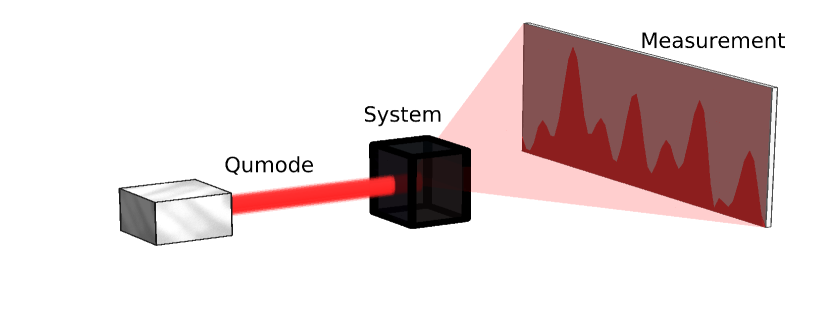
The qumode probing protocol consists of three components (see Fig. 1). The first of these is the system of interest, with state . The protocol does not in general need a particular form for the system or its state, and it may inhabit a discrete or continuous Hilbert space. As mentioned above, there is no need for a priori knowledge of this state, and in general this nescience is assumed. The second component is the continuous variable qumode, described by its quadratures and , often referred to as ‘position’ and ‘momentum’ [48]. We shall take these quadratures to be in their dimensionless form; that is, in terms of the creation and annihilation operators and of the mode, we have and .
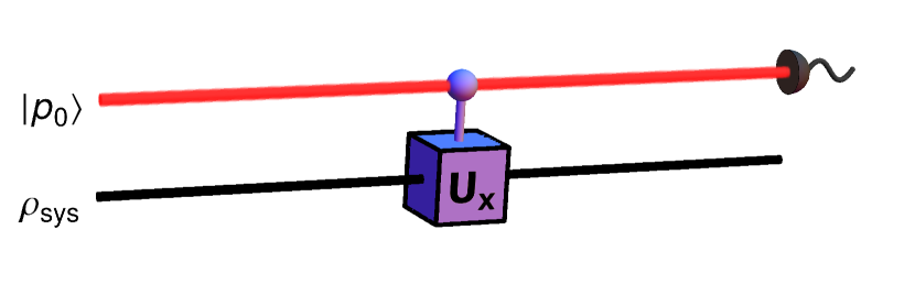
The final component is the interaction between system and qumode. We shall consider an interaction Hamiltonian of the form , where the first subspace belongs to the qumode, and the second the system [39]. Hence, the interaction acts on the system, with a strength that depends on the qumode position quadrature, with an overall coupling strength 111In principle the coupling strength can have a time dependence. Here we do not consider this beyond the straightforward binary on/off nature of a constant interaction strength.. The associated evolution operator (in natural units ) is , and thus the qumode is dephased in this quadrature, at a rate dependent on the the system operator , thence motivating the use of a phase estimation-type algorithm.
We label the eigenstates of the system operator as , with associated eigenvalues . Thus, when the system is in such an eigenstate, and the qumode in a quadrature eigenstate , the effect of the interaction can be written
| (1) |
In general, the qumode will be in a superposition of the quadrature eigenstates , and the system state can always be expressed in the basis defined by the eigenstates of : . Owing to the linearity of quantum mechanics, Eq. (1) can be extended to such states, and one can perform a partial trace over the system to obtain an expression for the qumode state after running the interaction for a time :
| (2) |
where analogous to the qubit probing protocols [29, 30], we define the dephasing function
| (3) |
where . This is resemblant of a characteristic function for the system operator, and is the crux of the probing protocol.
Let us now consider that after an interaction time a measurement is made of the qumode state. Inspired by the qubit-based protocols, we shall measure in a basis conjugate to that which defines the interaction Hamiltonian, here the momentum quadrature. Recall that these can be expressed in terms of the position eigenstates as . Correspondingly, using that , we have
| (4) |
where is the Fourier transform of . Thus, we see that the eigenvalues of the interaction Hamiltonian – and their associated probabilities – are imprinted into the final state of the qumode.
Before discussing the choice of initial probe state distribution , let us address a caveat to the above derivation. Namely, that we have neglected the presence of the natural evolution of the system under its bare Hamiltonian during the running of the protocol. For this to be valid, we require that the interaction occurs on timescales much faster than the natural evolution (), and that the natural evolution has negligible effect on the system state during the running of the protocol (), hence imposing a maximum allowable running time for the protocol. However, these restrictions are lifted when the bare Hamiltonian and the interaction Hamiltonian commute, in which case the natural evolution does not affect the outcome of the qumode measurement.
II.2 Initial probe state
Consider the idealised scenario where the qumode is initially prepared in an eigenstate of momentum ; . In this case, we find that , leading to
| (5) |
That is, the final state of the probe has a distribution that consists of sharp peaks, non-zero only at the points , where it takes values . The measurement of the qumode state hence directly samples the same distribution as that of a measurement of the operator on the state , with the mapping from qumode measurement outcomes to the spectrum of the system operator given by . With repeated measurements, one can then obtain an estimate of the probability distribution (and hence ). This thus allows for the estimation of moments of the system operator . Hence, by encoding a suitable operator associated with some observable of interest as our interaction Hamiltonian, we can use the protocol to determine the moments of with respect to the system state – effectively realising an ideal von Neumann measurement meter. It is worth noting that this does not require prior knowledge of the eigenvalues of the system operator, and further, that these can be determined from the qumode measurement outcomes. In contrast to the analogous qubit probing protocols, here all these properties can be obtained directly, without the need for post-processing of the measurement outcomes. This protocol is illustrated in Fig. 2.
However, this is an idealised model of the protocol, and in practice the qumode cannot be prepared in a true momentum quadrature eigenstate. Rather, one can only achieve approximations to this, with a finite level of squeezing in a given quadrature (the eigenstates corresponding to the limit of infinite squeezing). That is, we have a Gaussian uncertainty in the value of the momentum quadrature, centred on the desired , i.e.,
| (6) |
Here, corresponds to the dimensionless squeezing factor [39], parameterising the squeezing in the momentum quadrature 222Note that corresponds to the case of an unsqueezed coherent state, defined as the eigenstate of the annihilation operator; .. Inserting this in to Eq. (II.1), we find the final probability distribution for the qumode is given by
| (7) |
Indeed, the form of this distribution should not be too surprising – the smearing of the initial momentum distribution manifests in a smearing in the final distribution. This smearing is identical in the initial and final distributions, and is controlled by the squeezing factor. Specifically, the standard deviation of the final momentum distribution is given by , corresponding to a standard deviation for the system operator eigenvalues of . Thus, the precision to which we can measure the eigenvalues of can be increased by running the protocol for longer or increasing the coupling strength, or increasing the squeezing. This is analogous to a result found in the proposal for the power of one qumode computation [39], that one can trade off a decreased squeezing with increased running time , and vice versa.
While it is tempting to then conclude that these uncertainties in the final distribution can thus be negated by a sufficiently increased running time, this is not necessarily practical in general, due to the constraint imposed on for the effects of the system’s natural evolution to be neglected – as well as the inherent difficulties with maintaining coherence over long timescales. Ultimately, such practical considerations bound how small the spread can be made.
More generally, suppose we express the initial qumode state in the momentum eigenbasis as . We note that and are related by a basis change corresponding to a Fourier transform, i.e., . Thus, we can equivalently express Eq. (II.1) as ; the final distribution is a mixture of shifted versions of the initial momentum distribution, with weights given by the probability of each eigenstate of , and shifts proportional to the corresponding eigenvalue.
II.3 Candidate experimental platforms
The general form of the coupling Hamiltonian considered, , appears almost ubiquitiously in continuous-variable systems, as these typically couple through one of the quadratures of the qumode(s). Perhaps most famously, the basic building block of quantum light-matter interactions is the quantum Rabi model [48]:
| (8) |
where is the usual Pauli matrix [6], taking the role of the interaction Hamiltonian . The Hamiltonian was originally conceived as a description of a quantised light field interacting with a two-level system. One often finds this Hamiltonian in its simplified guise as the Jaynes-Cummings Hamiltonian, where the approximation is made to neglect the counter-rotating terms and ; nevertheless, systems described by this Hamiltonian are typically more accurately described by the full Rabi Hamiltonian. Moreover, though the Hamiltonian Eq. (8) contains only a coupling, it is possible to probe the spin operator in any chosen direction by an appropriate rotation of the individual spins prior to running the probing protocol, due to the rotation mapping the statistics of the desired direction onto the -axis (e.g. applying a Hadamard gate [6] to the system allows probing of ).
Both cavity [51, 52] and circuit [53, 54, 55, 56] quantum electrodynamics experiments consist of interactions between a continuous variable mode (cavity fields in the former, nanomechanical resonators in the latter) and a two-level system (atoms and superconducting qubits respectively), interacting through a quantum Rabi Hamiltonian Eq. (8) in the (ultra)strong coupling regime. Such setups operate in a regime where the qumode measurement resolution can be much finer than the differences between the interaction Hamiltonian eigenvalues, which for this example is of order unity. For example, in Ref. [54] the coupling between qubit and resonator gives , and the Q-factor of and resonance frequency of 8.2GHz leads to when the protocol is run for times of the order of the resonator lifetime. With the parameters of Ref. [52], we would have when is the cavity lifetime. Comparing with our example later, we see that this would offer a high degree of precision, with a very fine resolution of the spectrum.
While Eq. (8) makes it clear that the protocol can be used to probe moments of the spin operator of a two-level system, it can be applied more generally. First, the physical motivation and derivation of the Hamiltonian does not necessarily require that the system has only two states, and can be rederived for any number of states, by replacing with the appropriate spin operator for the number of states. Secondly, by illuminating an array of such systems with the same light field, the Hamiltonian becomes an interaction between the light field and the sum of the individual spin operators for each system, and thus probes moments of the total spin operator, as well as correlations between individual spins. This can be enhanced by tuning the optical geometry [57] such that different spins couple to the qumode with different strengths and phases. Further, when the individual spins are indistinguishable, they couple to the qumode as a single, collective spin operator, leading to the Dicke model [58, 59], which may be probed in a similar manner. Finally, higher-order light-matter interactions in the context of many-body systems often appear in such a form 333Note that this is not always apparent from a cursory inspection of the relevant Hamiltonians, as these are often derived with counter-rotating terms dropped – though a more full derivation will yield the appropriate form., such as in the case of cold atoms in optical cavities [61, 62].
We emphasise that the ‘momentum’ measurement made of the qumode is that of its canonical momentum quadrature, which does not necessarily correspond to a Newtonian momentum. Measurement of such quadratures is a highly routine procedure for photons in quantum optics [63], and can similarly performed for phonon qumodes formed by e.g., atomic or ionic motion [64, 42].
III Qumodes as Thermodynamical Probes
III.1 States in equilibrium
Consider a system that is known to be in a state of thermal equilibrium with respect to a Hamiltonian . Here, is the inverse temperature (we employ units in which Boltzmann’s constant ), and is the partition function. When the system component of the qumode interaction Hamiltonian is proportional to 444Note that in the circumstance where also coincides with the natural Hamiltonian of the system’s evolution , this also lifts the requirement that the qumode-system interaction takes place on short timescales relative to the natural evolution., we can use the qumode as a thermodynamical probe of the state.
Specifically, notice that the qumode probing protocol in this case will reveal for each eigenvalue of its respective probability in the state . Given that this eigenvalue has degeneracy , we can for each eigenvalue construct an equation of the form
| (9) |
which follows from taking the logarithm of the spectrum of . Let us assume that we know two of the eigenvalues and , and their associated degeneracies and respectively. By combining the associated Eq. (9) for both these eigenvalues, we obtain , i.e.,
| (10) |
By using the qumode to determine the associated and it thus provides a non-destructive means of determining the temperature of the system. Note that we do not need a priori knowledge of and , provided that we know the proportionality factor between and – the spectra will be similarly proportional to , and the former can be deduced from the output distribution. We also remark that a known constant shift in the (proportionally scaled) eigenvalues of one Hamiltonian relative to the other can similarly be accounted for.
Unlike traditional means of thermometry [66], we do not require thermal equilibrium to be established between the system and the probe – the temperature is measured through the shifts in the qumode state. Further, while similar schemes for measuring temperature using impurity probe qubits [30, 24] also do not require equilibriation, their accuracy is limited by the number of probes. This can be a limitation even for quantum thermometers that exploit advantages in precision using quantum metrology [67, 24]. In contrast, the precision of qumodes can also be enhanced by either increasing the squeezing factor, or increasing the interaction time or strength.
This approach requires that we can resolve between different eigenvalues of the interaction Hamiltonian , i.e., min(), or at least for the two eigenvalues used in Eq. (10) and their nearest neighbours. Otherwise, we must combine nearby eigenvalues and treat them as degenerate, in term limiting the precision to which the temperature can be estimated by the (scaled) uncertainty . The number of measurements required to determine the temperature to a given precision will scale inversely proportional to both the variance of the measurements of (set by , , and ) due to the finite width of the output distribution peaks, and the associated eigenstate probabilities and involved in Eq. (10).
Conversely, suppose we have knowledge of the temperature of the system (either beforehand, or using the above approach), and at least one of the degeneracies . Then, we can use qumode probing to deduce the remaining degeneracies by considering the ratio of the associated probabilities of the equilibrium state. Specifically, we have that
| (11) |
From this we are then able to reconstruct the full partition function . This offers access to several important thermodynamical quantities of interest [68], either directly, or by approximating derivatives of if we are able to slightly perturb the temperature. Amongst these quantities are the free energy (), heat capacity (), and entropies () – the latter two of which can be used to probe quantum critical points [69, 70].
Particularly valuable is the access reconstruction of provides to the free energy landscape of the system. Previously, proposals have been introduced, based either on the two-time measurement method, or using a qudit- [71] or qumode-based [42, 43] method, to sample from the distribution of work done on a system between two timepoints, where corresponds to the difference in energy before and after the evolution (indeed, the latter of these can be seen as an important special case application of our qumode-probing framework). Then, using the quantum counterpart [72, 73] of the Jaryzinski equality [74], the free energy difference is deduced from the work done – . However, these methods are not always efficient, particularly at low temperatures, or when large negative values of work are involved [71].In contrast, our method based on probing and directly still allows for the free energy to be recovered efficiently in those regimes.
III.2 Non-equilibrium thermodynamics
Qumodes can also be used to probe the thermodynamics of quantum systems that are perturbed far from equilibrium. In particular, we can probe the average work performed on a system due to a sudden quench in the interaction Hamiltonian – and moreover, determine the irreversible portion of this work [72, 75, 76], defined as the difference between , average work done on the system during the quench, and , the change in the free energy had the system evolved adiabatically from the thermal state of the initial interaction Hamiltonian to that of the final Hamiltonian. Interest in the irreversible component of work is motivated by the fluctuation theorems and its connections with various entropy measures [77, 72] – it is a widely-used measure of irreversibility, and has been shown to be a signature for some second-order phase transitions [78]. Note that the average work is also an interesting quantity to study in its own right, and its behaviour across a critical point has been connected to first-order quantum phase transitions [78].
The means of measuring average work and its irreversible component proceeeds as follows. Consider initial and final interaction Hamiltonians and , the former proportional to the system Hamiltonian , and the latter satisfying . For each of the interaction Hamiltonians we can apply the methods above to determine the free energies of their respective associated thermal states , and correspondingly, the difference in these free energies . Under a sudden quench, the system is unchanged and will remain in its initial thermal state , which is equivalent to a thermal state of at some effective inverse temperature . The proportionality between the system Hamiltonian , and the initial interaction Hamiltonian corresponds to the ratio between their eigenvalues , which also corresponds to the ratio of their associated temperatures .
Thus, the average work done by the quench is given by
| (12) |
where and are energies and probability amplitudes associated with the state for each of the interaction Hamiltonians . The second term corresponds to the average energy of the state with respect to the initial Hamiltonian, and so may be determined in the initial stage when we are calculating the associated free energy. The first term can be measured by using the qumode probing protocol to determine the and . Finally, we can calculate the irreversible component of the average work through .
Finally, we remark that we can also use qumode probes to find the overlaps of the ground states of a parameter-dependent Hamiltonian at two different values of the parameter . Such overlaps have been used to characterise regions of criticality defining quantum phase transitions, such as in the Dicke model [79]. Let denote the Hamiltonian when the parameter takes on a particular value , and let be the value of the parameter at the critical point. The overlap of the ground states associated with two values of the parameter and can be found using a concatenation of two qumode probing circuits. The first probing circuit is run using , and is post-selected on the qumode measurement resulting in the initial ground state energy, such that the state is left in the ground state of this Hamiltonian . We then probe this state using a second qumode, coupled with the interaction Hamiltonian . The probability that the qumode is found to have been shifted according to the ground state of this latter Hamiltonian then corresponds to , i.e., the desired overlap probability.
IV Example: Spin-1/2 Particle in Transverse Field
Consider a two level system with energies , for example, a spin-1/2 particle within a magnetic field of strength along the -direction. Consider further that the spin is subject to an additional field of strength along the -axis, such that the total Hamiltonian is given by
| (13) |
We now illustrate thermometry with a qumode by applying it to this example, when the system is thermalised to this Hamiltonian at a range of temperatures . Specifically, we simulate sampling from the distribution obtained by employing the probing protocol with a qumode initially prepared in a squeezed momentum state. We study a scenario where the interaction Hamiltonian is proportional to the system Hamiltonian, i.e., .
We will also, as an extra test of the protocol, mimic that the eigenvalues of and are unknown (but their relative proportionality is), and demand that the protocol also deduce these. We assume that it is known that there is one positive and one negative energy eigenvalue, such that the protocol will treat all measurements corresponding to a positive shift in momentum as being due to the negative eigenvalue, and vice versa. These are then averaged over to arrive at the deduced energy eigenvalues.
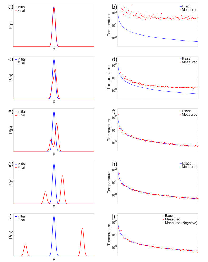
We examine the case that , . We consider temperatures in the range , with the extremes corresponding to the infinite temperature limit (), and a very low temperature limit (, ). We allow the qumode to make measurements (‘shots’) of the distribution, and combine the dependence on squeezing , coupling strength and interaction time in a single precision factor . To illustrate the effect of the precision, we plot the final distributions of the qumode state for at in Figs. 3(a,c,e,g,i) respectively.
The performance of the qumode at estimating the temperature of the spin for the prescibed range of temperatures is shown in Figs. 3(b,d,f,h,j) for each of the respective precisions. We see that at low precision the method overestimates the temperature. This is because the shift of the qumode momentum during the interaction is much smaller than the finite width of the initial distribution, and so a significant portion of the tails of the distribution are erroneously assigned to the wrong eigenvalue, creating the illusion of a more balanced population of the two states. We also observe that generally the accuracy is lower at high temperature (low ); this is because the exponential dependence of the state probabilities on renders a high degree of sensitivity in the deduced with respect to the measured probabilities at high temperature (where ). Indeed, when the measured probability for the excited state is greater than 1/2 (even if only to an arbitrarily small degree), the deduced temperature is negative. Ultimately, this can be ameliorated by using a larger number of shots that reduce the magnitude of the fluctuations in the measured probabilities. We remark that further numerical study (not shown) indicates that the number of shots is the limiting factor in the accuracy (rather than precision) for the shown plots at larger precision, and a visibly tighter clustering around the exact temperatues is observed for the measured temperatures at when the number of shots is increased to .
V Conclusion
Properties of quantum systems may be imprinted onto continuous variable qumode ancillae, allowing for non-destructive probing of the system. For an appropriate choice of interaction operator and initial qumode state, the occupation probabilities of the desired observable’s eigenstates with respect to the system state are mapped directly on to the qumode state. The qumode state then behaves according to the same statistics as this operator, and thus measurement of the qumode reproduces the same result as a direct measurement of the system would, while avoiding particular drawbacks associated with direct measurements of practical implementations of quantum technologies. We have shown that this method of probing has a strong potential for use in probing the thermodynamics of quantum systems, allowing access to many quantities of interest, particularly in the context of cold atom quantum simulators.
For systems in equilibrium, qumode probing can be used for thermometry of the system temperature, as well as reconstruction of the partition function, from which many other thermodynamical quantities of interest can be deduced. Moreover, for systems outside of equilibrium, qumodes can be used to probe work and free energy differences under evolutions of the system and its Hamiltonian. As the basic form of the interaction is almost synonymous with the form of quantum light-matter interactions, there is a significant scope of applicability of these results, particularly given that the necessary parameter regimes can be achieved in current experiments. Indeed, we remark that while several of our results require the system component of the interaction Hamiltonian to be proportional to the thermalising Hamiltonian of the system, this is not an unrealistic challenge particularly in systems driven by their interactions with light or other similar environments, especially in the strong-coupling regime. With the high degree of tunability of the specific form of the interaction offered by optical setups, qumode probing promises to be a valuable tool in the experimental characterisation of many-body quantum systems.
Acknowledgements.
The authors acknowledge financial support from Grants No. FQXi-RFP-1809 and No. FQXi-RFP-IPW-1903 from the Foundational Questions Institute and Fetzer Franklin Fund (a donor advised fund of Silicon Valley Community Foundation), the University of Manchester Dame Kathleen Ollerenshaw Fellowship, the Imperial College Borland Fellowship in Mathematics, the Singapore Ministry of Education Tier 2 Grant MOE-T2EP50221-0005, the Singapore Ministry of Education Tier 1 Grant RG77/22, and the National Research Foundation, Singapore, and Agency for Science, Technology and Research (A*STAR) under its QEP2.0 programme (NRF2021-QEP2-02-P06, and funding from the Science and Technology Program of Shanghai, China (21JC1402900). Any opinions, findings and conclusions or recommendations expressed in this material are those of the authors and do not reflect the views of National Research Foundation or the Ministry of Education Singapore. T. J. E. and N. L. thank the Centre for Quantum Technologies for their hospitality. Data Availability. Data sharing not applicable to this article as no datasets were generated or analysed during the current study. Author Contributions. All authors contributed to the research and writing of the manuscript. Competing Interests. The authors declare no competing interests.References
- Bloch et al. [2012] I. Bloch, J. Dalibard, and S. Nascimbène, Quantum simulations with ultracold quantum gases, Nat. Phys. 8, 267 (2012).
- Blatt and Roos [2012] R. Blatt and C. F. Roos, Quantum simulations with trapped ions, Nat. Phys. 8, 277 (2012).
- Clarke and Wilhelm [2008] J. Clarke and F. K. Wilhelm, Superconducting quantum bits, Nature 453, 1031 (2008).
- Raimond et al. [2001] J. M. Raimond, M. Brune, and S. Haroche, Manipulating quantum entanglement with atoms and photons in a cavity, Rev. Mod. Phys. 73, 565 (2001).
- Monroe [2002] C. Monroe, Quantum information processing with atoms and photons, Nature 416, 238 (2002).
- Nielsen and Chuang [2010] M. A. Nielsen and I. L. Chuang, Quantum Computation and Quantum Information (Cambridge University Press, 2010).
- Giovannetti et al. [2011] V. Giovannetti, S. Lloyd, and L. Maccone, Advances in quantum metrology, Nat. Photon. 5, 222 (2011).
- Haroche and Raimond [2013] S. Haroche and J. M. Raimond, Exploring the Quantum: Atoms, Cavities, and Photons (OUP Oxford, 2013).
- Lewenstein et al. [2012] M. Lewenstein, A. Sanpera, and V. Ahufinger, Ultracold Atoms in Optical Lattices: Simulating Quantum Many-Body Systems (Oxford University Press, Oxford, England, 2012).
- Johnson et al. [2014] T. H. Johnson, S. Clark, and D. Jaksch, What is a quantum simulator?, EPJ Quantum Technology 1, 10 (2014).
- Daley et al. [2022] A. J. Daley, I. Bloch, C. Kokail, S. Flannigan, N. Pearson, M. Troyer, and P. Zoller, Practical quantum advantage in quantum simulation, Nature 607, 667 (2022).
- Cao et al. [2019] Y. Cao, J. Romero, J. P. Olson, M. Degroote, P. D. Johnson, M. Kieferová, I. D. Kivlichan, T. Menke, B. Peropadre, N. P. Sawaya, S. Sim, L. Veis, and A. Aspuru-Guzik, Quantum chemistry in the age of quantum computing, Chemical Reviews 119, 10856 (2019).
- Hadzibabic et al. [2003] Z. Hadzibabic, S. Gupta, C. A. Stan, C. H. Schunck, M. W. Zwierlein, K. Dieckmann, and W. Ketterle, Fiftyfold improvement in the number of quantum degenerate fermionic atoms, Phys. Rev. Lett. 91, 160401 (2003).
- Altman et al. [2004] E. Altman, E. Demler, and M. D. Lukin, Probing many-body states of ultracold atoms via noise correlations, Phys. Rev. A 70, 013603 (2004).
- Fölling et al. [2005] S. Fölling, F. Gerbier, A. Widera, O. Mandel, T. Gericke, and I. Bloch, Spatial quantum noise interferometry in expanding ultracold atom clouds, Nature 434, 481 (2005).
- Bloch et al. [2008] I. Bloch, J. Dalibard, and W. Zwerger, Many-body physics with ultracold gases, Rev. Mod. Phys. 80, 885 (2008).
- Recati et al. [2005] A. Recati, P. O. Fedichev, W. Zwerger, J. Von Delft, and P. Zoller, Atomic quantum dots coupled to a reservoir of a superfluid Bose-Einstein condensate, Phys. Rev. Lett. 94, 40404 (2005).
- Bruderer and Jaksch [2006] M. Bruderer and D. Jaksch, Probing BEC phase fluctuations with atomic quantum dots, New J. Phys. 8, 87 (2006).
- Goold et al. [2011] J. Goold, T. Fogarty, N. L. Gullo, M. Paternostro, and T. Busch, Orthogonality catastrophe as a consequence of qubit embedding in an ultracold fermi gas, Phys. Rev. A 84, 063632 (2011).
- Knap et al. [2012] M. Knap, A. Shashi, Y. Nishida, A. Imambekov, D. A. Abanin, and E. Demler, Time-dependent impurity in ultracold fermions: Orthogonality catastrophe and beyond, Phys. Rev. X 2, 041020 (2012).
- Haikka et al. [2013] P. Haikka, S. McEndoo, and S. Maniscalco, Non-Markovian probes in ultracold gases, Phys. Rev. A 87, 012127 (2013).
- Mazzola et al. [2013] L. Mazzola, G. De Chiara, and M. Paternostro, Measuring the characteristic function of the work distribution, Phys. Rev. Lett. 110, 230602 (2013).
- Dorner et al. [2013] R. Dorner, S. R. Clark, L. Heaney, R. Fazio, J. Goold, and V. Vedral, Extracting quantum work statistics and fluctuation theorems by single-qubit interferometry, Phys. Rev. Lett. 110, 230601 (2013).
- Sabín et al. [2014] C. Sabín, A. White, L. Hackermuller, and I. Fuentes, Impurities as a quantum thermometer for a Bose-Einstein condensate, Sci. Rep. 4, 6436 (2014).
- Fusco et al. [2014] L. Fusco, S. Pigeon, T. J. G. Apollaro, A. Xuereb, L. Mazzola, M. Campisi, A. Ferraro, M. Paternostro, and G. De Chiara, Assessing the nonequilibrium thermodynamics in a quenched quantum many-body system via single projective measurements, Phys. Rev. X 4, 031029 (2014).
- Batalhão et al. [2014] T. B. Batalhão, A. M. Souza, L. Mazzola, R. Auccaise, R. S. Sarthour, I. S. Oliveira, J. Goold, G. De Chiara, M. Paternostro, and R. M. Serra, Experimental reconstruction of work distribution and study of fluctuation relations in a closed quantum system, Phys. Rev. Lett. 113, 140601 (2014).
- Hangleiter et al. [2015] D. Hangleiter, M. T. Mitchison, T. H. Johnson, M. Bruderer, M. B. Plenio, and D. Jaksch, Nondestructive selective probing of phononic excitations in a cold Bose gas using impurities, Phys. Rev. A 91, 013611 (2015).
- Cosco et al. [2017] F. Cosco, M. Borrelli, F. Plastina, and S. Maniscalco, Momentum-resolved and correlation spectroscopy using quantum probes, Phys. Rev. A 95, 053620 (2017).
- Elliott and Johnson [2016] T. J. Elliott and T. H. Johnson, Nondestructive probing of means, variances, and correlations of ultracold-atomic-system densities via qubit impurities, Phys. Rev. A 93, 043612 (2016).
- Johnson et al. [2016] T. H. Johnson, F. Cosco, M. T. Mitchison, D. Jaksch, and S. R. Clark, Thermometry of ultracold atoms via nonequilibrium work distributions, Phys. Rev. A 93, 053619 (2016).
- Bermudez et al. [2017] A. Bermudez, G. Aarts, and M. Müller, Quantum sensors for the generating functional of interacting quantum field theories, Phys. Rev. X 7, 041012 (2017).
- Benedetti et al. [2018] C. Benedetti, F. Salari Sehdaran, M. H. Zandi, and M. G. A. Paris, Quantum probes for the cutoff frequency of Ohmic environments, Phys. Rev. A 97, 012126 (2018).
- Bentine et al. [2017] E. Bentine, T. L. Harte, K. Luksch, A. J. Barker, J. Mur-Petit, B. Yuen, and C. J. Foot, Species-selective confinement of atoms dressed with multiple radiofrequencies, J. Phys. B 50, 094002 (2017).
- Lloyd and Braunstein [1999] S. Lloyd and S. L. Braunstein, Quantum computation over continuous variables, Phys. Rev. Lett. 82, 1784 (1999).
- Braunstein and Van Loock [2005] S. L. Braunstein and P. Van Loock, Quantum information with continuous variables, Rev. Mod. Phys. 77, 513 (2005).
- Furusawa and Van Loock [2011] A. Furusawa and P. Van Loock, Quantum teleportation and entanglement: A hybrid approach to optical quantum information processing (John Wiley & Sons, 2011).
- Weedbrook et al. [2012] C. Weedbrook, S. Pirandola, R. García-Patrón, N. J. Cerf, T. C. Ralph, J. H. Shapiro, and S. Lloyd, Gaussian quantum information, Rev. Mod. Phys. 84, 621 (2012).
- Andersen et al. [2015] U. L. Andersen, J. S. Neergaard-Nielsen, P. van Loock, and A. Furusawa, Hybrid discrete-and continuous-variable quantum information, Nat. Phys. 11, 713 (2015).
- Liu et al. [2016] N. Liu, J. Thompson, C. Weedbrook, S. Lloyd, V. Vedral, M. Gu, and K. Modi, Power of one qumode for quantum computation, Phys. Rev. A 93, 052304 (2016).
- von Neumann [1932] J. von Neumann, Mathematische Grundlagen der Quantenmechanik (Springer, 1932).
- Brune et al. [1996] M. Brune, E. Hagley, J. Dreyer, X. Maitre, A. Maali, C. Wunderlich, J. M. Raimond, and S. Haroche, Observing the progressive decoherence of the “meter” in a quantum measurement, Phys. Rev. Lett. 77, 4887 (1996).
- Cerisola et al. [2017] F. Cerisola, Y. Margalit, S. Machluf, A. J. Roncaglia, J. P. Paz, and R. Folman, Using a quantum work meter to test non-equilibrium fluctuation theorems, Nat. Comm. 8, 1241 (2017).
- Ahmad and Smith [2022] S. A. Ahmad and A. R. Smith, Finite-resolution ancilla-assisted measurements of quantum work distributions, Physical Review A 105, 052411 (2022).
- Vogel and Risken [1989] K. Vogel and H. Risken, Determination of quasiprobability distributions in terms of probability distributions for the rotated quadrature phase, Phys. Rev. A 40, 2847 (1989).
- Hradil [1997] Z. Hradil, Quantum-state estimation, Phys. Rev. A 55, R1561 (1997).
- D’Ariano and Presti [2003] G. M. D’Ariano and P. L. Presti, Imprinting complete information about a quantum channel on its output state, Phys. Rev. Lett. 91, 047902 (2003).
- Paris and Řeháček [2004] M. Paris and J. Řeháček, Quantum State Estimation (Springer, 2004).
- Gerry and Knight [2005] C. Gerry and P. Knight, Introductory Quantum Optics (Cambridge University Press, 2005).
- Note [1] In principle the coupling strength can have a time dependence. Here we do not consider this beyond the straightforward binary on/off nature of a constant interaction strength.
- Note [2] Note that corresponds to the case of an unsqueezed coherent state, defined as the eigenstate of the annihilation operator; .
- Gleyzes et al. [2007] S. Gleyzes, S. Kuhr, C. Guerlin, J. Bernu, S. Deleglise, U. B. Hoff, M. Brune, J.-M. Raimond, and S. Haroche, Quantum jumps of light recording the birth and death of a photon in a cavity, Nature 446, 297 (2007).
- Hamsen et al. [2017] C. Hamsen, K. N. Tolazzi, T. Wilk, and G. Rempe, Two-photon blockade in an atom-driven cavity QED system, Phys. Rev. Lett. 118, 133604 (2017).
- LaHaye et al. [2009] M. D. LaHaye, J. Suh, P. M. Echternach, K. C. Schwab, and M. L. Roukes, Nanomechanical measurements of a superconducting qubit, Nature 459, 960 (2009).
- Forn-Díaz et al. [2010] P. Forn-Díaz, J. Lisenfeld, D. Marcos, J. J. García-Ripoll, E. Solano, C. J. P. M. Harmans, and J. E. Mooij, Observation of the Bloch-Siegert shift in a qubit-oscillator system in the ultrastrong coupling regime, Phys. Rev. Lett. 105, 237001 (2010).
- O’Connell et al. [2010] A. D. O’Connell, M. Hofheinz, M. Ansmann, R. C. Bialczak, M. Lenander, E. Lucero, M. Neeley, D. Sank, H. Wang, M. Weides, J. Wenner, M. J. M, and C. A. N, Quantum ground state and single-phonon control of a mechanical resonator, Nature 464, 697 (2010).
- Yoshihara et al. [2017] F. Yoshihara, T. Fuse, S. Ashhab, K. Kakuyanagi, S. Saito, and K. Semba, Superconducting qubit-oscillator circuit beyond the ultrastrong-coupling regime, Nat. Phys. 13, 44 (2017).
- Elliott et al. [2015] T. J. Elliott, W. Kozlowski, S. F. Caballero-Benitez, and I. B. Mekhov, Multipartite entangled spatial modes of ultracold atoms generated and controlled by quantum measurement, Phys. Rev. Lett. 114, 113604 (2015).
- Baumann et al. [2010] K. Baumann, C. Guerlin, F. Brennecke, and T. Esslinger, Dicke quantum phase transition with a superfluid gas in an optical cavity, Nature 464, 1301 (2010).
- Landig et al. [2016] R. Landig, L. Hruby, N. Dogra, M. Landini, R. Mottl, T. Donner, and T. Esslinger, Quantum phases from competing short-and long-range interactions in an optical lattice, Nature (2016).
- Note [3] Note that this is not always apparent from a cursory inspection of the relevant Hamiltonians, as these are often derived with counter-rotating terms dropped – though a more full derivation will yield the appropriate form.
- Ritsch et al. [2013] H. Ritsch, P. Domokos, F. Brennecke, and T. Esslinger, Cold atoms in cavity-generated dynamical optical potentials, Rev. Mod. Phys. 85, 553 (2013).
- Elliott and Mekhov [2016] T. J. Elliott and I. B. Mekhov, Engineering many-body dynamics with quantum light potentials and measurements, Physical Review A 94, 013614 (2016).
- Slusher et al. [1985] R. E. Slusher, L. W. Hollberg, B. Yurke, J. C. Mertz, and J. F. Valley, Observation of squeezed states generated by four-wave mixing in an optical cavity, Physical Review Letters 55, 2409 (1985).
- Bastin et al. [2006] T. Bastin, J. von Zanthier, and E. Solano, Measure of phonon-number moments and motional quadratures through infinitesimal-time probing of trapped ions, Journal of Physics B: Atomic, Molecular and Optical Physics 39, 685 (2006).
- Note [4] Note that in the circumstance where also coincides with the natural Hamiltonian of the system’s evolution , this also lifts the requirement that the qumode-system interaction takes place on short timescales relative to the natural evolution.
- Correa et al. [2015] L. A. Correa, M. Mehboudi, G. Adesso, and A. Sanpera, Individual quantum probes for optimal thermometry, Phys. Rev. Lett. 114, 220405 (2015).
- Stace [2010] T. M. Stace, Quantum limits of thermometry, Phys. Rev. A 82, 011611 (2010).
- Glazer and Wark [2002] M. Glazer and J. Wark, Statistical Mechanics (Oxford University Press, 2002).
- Fradkin and Moore [2006] E. Fradkin and J. E. Moore, Entanglement entropy of 2d conformal quantum critical points: hearing the shape of a quantum drum, Physical Review Letters 97, 050404 (2006).
- Liang et al. [2015] T. Liang, S. M. Koohpayeh, J. W. Krizan, T. M. McQueen, R. J. Cava, and N. P. Ong, Heat capacity peak at the quantum critical point of the transverse Ising magnet CoNb2O6, Nat. Comm. 6 (2015).
- Roncaglia et al. [2014] A. J. Roncaglia, F. Cerisola, and J. P. Paz, Work measurement as a generalized quantum measurement, Phys Rev. Lett. 113, 250601 (2014).
- Tasaki [2000] H. Tasaki, Jarzynski relations for quantum systems and some applications, arXiv preprint arXiv:cond-mat/0009244 (2000).
- Mukamel [2003] S. Mukamel, Quantum extension of the Jarzynski relation: analogy with stochastic dephasing, Phys. Rev. Lett. 90, 170604 (2003).
- Jarzynski [1997] C. Jarzynski, Nonequilibrium equality for free energy differences, Phys. Rev. Lett. 78, 2690 (1997).
- Campisi et al. [2011] M. Campisi, P. Hänggi, and P. Talkner, Colloquium: Quantum fluctuation relations: Foundations and applications, Rev. Mod. Phys. 83, 771 (2011).
- Dorner et al. [2012] R. Dorner, J. Goold, C. Cormick, M. Paternostro, and V. Vedral, Emergent thermodynamics in a quenched quantum many-body system, Phys. Rev. Lett. 109, 160601 (2012).
- Deffner and Lutz [2010] S. Deffner and E. Lutz, Generalized Clausius inequality for nonequilibrium quantum processes, Phys. Rev. Lett. 105, 170402 (2010).
- Mascarenhas et al. [2014] E. Mascarenhas, H. Bragança, R. Dorner, M. F. Santos, V. Vedral, K. Modi, and J. Goold, Work and quantum phase transitions: Quantum latency, Phys. Rev. E 89, 062103 (2014).
- Zanardi and Paunković [2006] P. Zanardi and N. Paunković, Ground state overlap and quantum phase transitions, Phys. Rev. E 74, 031123 (2006).