Network Dynamics of Innovation Processes

Abstract

We introduce a model for the emergence of innovations, in which cognitive processes are described as random walks on the network of links among ideas or concepts, and an innovation corresponds to the first visit of a node. The transition matrix of the random walk depends on the network weights, while in turn the weight of an edge is reinforced by the passage of a walker. The presence of the network naturally accounts for the mechanism of the “adjacent possible,” and the model reproduces both the rate at which novelties emerge and the correlations among them observed empirically. We show this by using synthetic networks and by studying real data sets on the growth of knowledge in different scientific disciplines. Edge-reinforced random walks on complex topologies offer a new modeling framework for the dynamics of correlated novelties and are another example of coevolution of processes and networks.

Creativity and innovation are the underlying forces driving the growth of our society and economy. Studying creative processes and understanding how new ideas emerge and how novelties can trigger further discoveries is therefore fundamental if we want to devise effective interventions to nurture the success and sustainable growth of our society. Recent empirical studies have investigated the emergence of novelties in a wide variety of different contexts, including science Rzhetsky et al. (2015); Sinatra et al. (2016), knowledge and information Andjelković et al. (2016); Rodi et al. (2017), goods and products Saracco et al. (2015), language Puglisi et al. (2008), and also gastronomy Fink et al. (2016) and cinema Sreenivasan (2013). In particular, the authors of Refs. Tria et al. (2014); Monechi et al. (2017a); Cattuto et al. (2007a, b) have looked at different types of temporally ordered sequences of data, such as sequences of words, songs, Wikipages and tags to study how the number $S(t)$ of novelties grows with the length of the sequence $t$. They have found that the Heaps’ law, i.e. a power-law behaviour $S(t)\sim t^{\beta}$ originally introduced to describe the number of distinct words in a text document Heaps (1978), applies to different contexts, producing different values of $\beta<1$. In parallel to the empirical analyses, various models have been proposed to reproduce the innovation dynamics in different domains, such as linguistics Gerlach and Altmann (2013); Lü et al. (2013), social systems Dankulov et al. (2015), or self-organized criticality (SOC) Tadic et al. (2017). Other approaches have modeled the emergence of innovation as an evolutionary process, such as the Schumpeterian economic dynamics proposed by Thurner et al. Thurner et al. (2010) and the evolutionary game among innovators and developers proposed by Armano and Javarone Armano and Javarone (2017). Urn models are another useful framework to study innovation processes in evolutionary biology, chemistry, sociology, economy and text analysis Simkin and Roychowdhury (2011); Marengo and Zeppini (2016). In the classic Polya urn model Hoppe (1984); Pólya (1930), a temporal sequence of discoveries can be generated by drawing balls from an urn that contains all possible inventions. Several variations have been proposed, such as the urn model with memory, to reproduce the dynamics of collaborative tagging Cattuto et al. (2007a), or the more recent model by Tria and co-workers Tria et al. (2014); Loreto et al. (2016), which adds the concept of the adjacent possible Kauffman (1996); Gravino et al. (2016) to the reinforcement mechanism of the Polya’s urn framework.

In this letter, we propose to model the dynamical mechanisms leading to discoveries and innovations as an edge-reinforced random walk (ERRW) on an underlying network of relations among concepts and ideas. Random walks on complex networks Albert and Barabási (2002); Newman (2003); Boccaletti et al. (2006); Barrat et al. (2008); Latora et al. (2017) have been studied at length Masuda et al. (2016). In the context of innovation, they have been used to build exploration models for social annotation Cattuto et al. (2009), music album popularity Monechi et al. (2017b), knowledge acquisition de Arruda et al. (2017), human language complexity Allegrini et al. (2004) and evolution in research interests Jia et al. (2017). A special class of random walks are those with reinforcement Gómez-Gardeñes and Latora (2008); Agliari et al. (2012); Pemantle et al. (2007), which have been successfully applied to biology Boyer and Solis-Salas (2014) and mobility Choi et al. (2012); Szell et al. (2012). In particular, the concept of edge reinforcement Merkl and Rolles (2006); Keane et al. (2000); Foster et al. (2009) was introduced in the mathematical literature by Coppersmith and Diaconis Coppersmith and Diaconis (1987). Here, we will use ERWWs to mimic how different concepts are explored moving from a concept to an adjacent one in the network, with innovations being represented, in this framework, by the first discovery of nodes. As supported by empirical observations, we expect indeed the walkers to move more frequently among already known concepts and, from time to time, to discover new nodes. For this reason, we introduce and study a model in which the network is co-evolving with the dynamical process taking place over it. In our model, (i) random walkers move over a network with assigned topology and whose edge weights represent the strength of concept associations, and (ii) the network evolves in time through a reinforcement mechanism in which the weight of an edge is increased every time the edge is traversed by a walker, making traversed edges more likely to be traversed again. As we will show, this model is able to reproduce the statistical properties observed in real data of innovation processes, i. e., the Heaps’ law Heaps (1978), and by tuning the amount of reinforcement it can give rise to different scaling exponents. Furthermore, correlations in the temporal sequences of visited concepts and innovations will appear as a natural consequence of the interplay between the network topology and the reinforcement mechanism that controls the exploration dynamics.

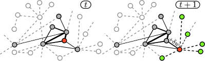
Figure 1: Edge-reinforced random walks (ERRWs) produce a coevolution of the network with the dynamics of the walkers. At time $t$ the walker is on the red node and has already visited the gray nodes, while the shaded nodes are still unexplored. The widths of edges are proportional to their weights. At time $t+1$ the walker has moved to a neighbor (red) with probability as in Eq. (1), and the weight of the used edge has been reinforced by $\delta w$. At this point, the walker will preferentially go back, although it can also access the set of “adjacent possible” (green).

Model. Let us consider a random walker over a weighted connected graph $G(\mathcal{V},\mathcal{E})$, where $\mathcal{V}$ and $\mathcal{E}$ are, respectively, a set of $N=|\mathcal{V}|$ nodes and a set of $K=|\mathcal{E}|$ links. Each node of the graph represents a concept or an idea, and the presence of a link $(i,j)$ denotes the existence of a direct relation between two concepts $i$ and $j$. The values of $N$ and $K$ and the topology of the network are assumed to be fixed, while the weights of the edges can change in time according to the dynamics of the walker, which, as we will see below, is in turn influenced by the underlying network. The graph at time $t$, with $t=0,1,2,\ldots$, is fully described by the non-negative time-dependent adjacency matrix $W^{t}\equiv\{w^{t}_{ij}\}$, where the value $w^{t}_{ij}$ is different from 0 if the two concepts $i$ and $j$ are related, and quantifies the strength of the relationship at time $t$. We initialize the network assuming that at time $t=0$ all the edges have the same weight, namely $w^{0}_{ij}=1\leavevmode\nobreak\ \forall(i,j)\in\mathcal{E}$. The dynamics of the walkers is defined as follows: at each time step $t$, a walker at node $i$ jumps to a randomly chosen neighboring node $j$ with a probability proportional to the weight of the connecting edge. Formally, the probability of going from node $i$ to node $j$ at time $t$ is:

$$\text{Prob}^{t}(i\rightarrow j)=\pi^{t}_{ji}=\frac{w^{t}_{ij}}{\sum_{l}w^{t}_{il}}$$ (1)

where the time-dependent transition probability matrix $\Pi^{t}\equiv\{\pi^{t}_{ij}\}$ depends on the weights of all links at time $t$ Cover and Thomas (2012). The transition probabilities satisfy the normalization $\sum_{j}\pi^{t}_{ji}=1$ $\forall i,t$, and we assume that $G$ has no self-loops, so that the walker changes position at each time step. On the other hand, the network coevolves with the random walk process, since every time a walker traverses a link, it increases its weight by a quantity $\delta w>0$, as illustrated in Fig. 1. This mechanism mimics the fact that the relation between two concepts is reinforced every time the two concepts are associated by a cognitive process. Formally, the dynamics of the network is the following. Every time an edge $(i,j)\in\mathcal{E}$ is traversed at time $t$, the associated weight is reinforced as

$$w^{t+1}_{ij}=w^{t}_{ij}+\delta w$$ (2)

The quantity $\delta w$, called reinforcement, is the only tunable parameter of the model. The idea of a walker preferentially returning on its steps is in line with the classical rich-get-richer paradigm, which has been extensively used in the network literature to grow scale-free graphs Barabási and Albert (1999), and is here implemented in terms of reinforcement of the edges, instead of using a random walk biased on some properties of the nodes Gómez-Gardeñes and Latora (2008); Bonaventura et al. (2014); Sood and Grassberger (2007).

The coevolution of network and walker motion induces a long-term memory in the trajectories which reproduces, as we will show below, the empirically observed correlations in the dynamics of innovations Tria et al. (2014). In fact, if $i_{t}$ is a realization of the random variable $X_{t}$ denoting the position of the walker at time $t$, the conditional probability $\text{Prob}\left[X_{t+1}=i|i_{0},i_{1},\ldots,i_{t}\right]$ that, at time step $t+1$, the walker is at node $i$, after a trajectory $\mathcal{S}=(i_{0},i_{1},i_{2},\ldots,i_{t})$, depends on the whole history of the visited nodes, namely on the frequency but also on the precise order in which they have been visited Szell et al. (2012). The strongly non-Markovian Gardiner (1985) nature of the random walks comes indeed from the fact that the transition matrix $\Pi^{t}$ coevolves with the rearrangement of the weights. This makes our approach fundamentally different from the other models based on Polya-like processes. For instance, in the Tria et al. urn model Tria et al. (2014), where an innovation corresponds to the extraction of a ball of a new color, the probability of extracting a given color (colors correspond to node labels in our model) at time $t+1$ only depends on the number of times each color has been extracted up to time $t$, and not on the precise sequence of colors. Moreover, the use of an underlying network (see Fig. 1) is a natural way to include the concept of the adjacent possible in our model, without the need of a triggering mechanism and further parameters, which are instead necessary in the UM (balls of new colors added into the urn whenever a color is drawn out for the first time) and in its mapping in terms of growing graphs considered in SI of Refs. Tria et al. (2014); Monechi et al. (2017a).

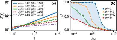
Figure 2: ERRW on SW networks with $N=10^{5}$ and $m=1$. (a) Heaps’ law and associated exponents $\beta$ obtained for different values of reinforcement $\delta w$ on a network with $p=0.02$. (b) Exponent $\beta$ as a function of the reinforcement $\delta w$ for networks with different rewiring probabilities $p$.

Results. We first test our model on synthetic networks, and then consider a real case where the underlying network of relations among concepts can be directly accessed and used. As a first experiment, based on the idea that concepts are organized in dense clusters connected by few long-range links, we model the relations among concepts as a small-world network (SW) Watts (1999). Our choice is supported by recent results on small-world properties of word associations Gravino et al. (2012), language networks Motter et al. (2002) and semantic networks of creative people Benedek et al. (2017). To construct SW networks we use the procedure proposed in Ref. Newman and Watts (1999). Namely, we start with a ring of $N$ nodes, each connected to its $2m$ nearest neighbors, and then we add, with a tunable probability $p$, a new random edge for each of the edges of the ring. The first thing we want to investigate is the Heaps’ law for the rate at which novelties happen Heaps (1978); Tria et al. (2014). We therefore looked at how the number of distinct nodes $S(t)$ in a sequence $\mathcal{S}$ generated by a walker grows as a function of length of the sequence $t$. Figure 2(a) shows the curves $S(t)$ obtained by averaging over different realizations of a ERRW process with reinforcement $\delta w$ on a SW network with rewiring probability $p=0.02$. All the curves can be well fitted by a power law $S(t)\sim t^{\beta}$, with an exponent $\beta$ which decreases when the reinforcement $\delta w$ increases. Finding the average number of distinct sites visited by a random walker is a well-known problem in the case of graphs without reinforcement. In particular, it has been proven that, in the absence of reinforcement, the average number of distinct sites $S(t)$ visited in $t$ steps scales as $S^{\text{ring}}(t)\sim\left(8t/\pi\right)^{{1/2}}$ Dvoretzky and Erdös (1951) in one-dimensional lattices and as $S^{\text{ER}}(t)\sim t$ De Bacco et al. (2015) in Erdős-Rényi random graphs Erdös and Rényi (1959). The transition between these two regimes has been investigated in Refs. Jasch and Blumen (2001); Lahtinen et al. (2001); Almaas et al. (2003) for SW networks with different values of $p$. Figure 2(b) reports the fitted values of the exponent $\beta$ obtained in the case of ERRW with different strength of reinforcement. The four curves refer to SW networks with rewiring probabilities $p=0,0.02,0.1$, and $1$. Notice that the previously known results, $\beta^{\text{ring}}=1/2$ and $\beta^{\text{ER}}=1$, are recovered as limits of the two curves relative to $p=0$ and $p=1$ when $\delta w\to 0$. Furthermore, for values of $p$ in the small-world regime Barrat and Weigt (2000), it is possible to get values of $\beta$ spanning the entire range $[0,1]$ by tuning the amount of reinforcement $\delta w$. This means that the reinforcement mechanism we propose is able to reproduce all the Heaps’ exponents empirically observed Tria et al. (2014).

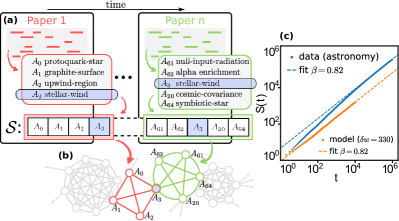
Figure 3: Growth of knowledge in science. (a) For each scientific field, an empirical sequence of scientific concepts $\mathcal{S}$ is extracted from the abstracts of the temporally ordered sequence of papers. (b) The network of relations among concepts is constructed by linking two concepts if they appear in the same abstract. The network is then used as the underlying structure for the ERRW model. (c) The model is tuned to the empirical data by choosing the value of the reinforcement $\delta w$ that reproduces the Heaps’ exponent $\beta$ associated to $\mathcal{S}$.

Cognitive growth of science. To show how the model works in a real case, we have extracted the empirical curves $S(t)$ associated with a discovery process on an underlying network whose topology can be directly accessed. Specifically, we studied the growth of knowledge in modern science by analyzing 20 years (1991-2010) of scientific articles in four different disciplines, namely, astronomy, ecology, economy and mathematics. Articles were taken from core journals in these four fields, and bibliographic records were downloaded from the Web of Science database (details in Ref. Milojević (2012)). From a text analysis of each abstract, we have extracted relevant concepts as multiword phrases Milojević (2015) and constructed, as in Fig. 3(a), the real temporal sequence $\mathcal{S}$ in each field from the publication date of the papers. Figure 3(c) shows that the number $S(t)$ of novel concepts in astronomy grows with the length $t$ of $\mathcal{S}$ as a power law with a fitted exponent $\beta=0.82$. Together with the real exploration sequences we have also extracted, as illustrated in Fig. 3(b), the underlying networks of relations among concepts et al. (2013) from their co-occurrences in the abstracts, so that we do not need to rely on synthetic small-world topologies, or on the graph version of the UM (see SI of Refs. Tria et al. (2014); Monechi et al. (2017a)). Table 1 reports basic properties, such as number of nodes $N$, average node degree $\langle k\rangle$, characteristic path length $L$ and clustering coefficient $C$, for the largest components of the four networks we have constructed. Notice that different disciplines exhibit values of $\langle k\rangle$ ranging from 19 for mathematics to 172 for astronomy, but all of them have high values of $C$ and low $L$. We have then run the ERRW on each of the four networks, tuning the strength of the reinforcement $\delta w$, the only parameter of the model, so that the obtained curves for the growth of the number of distinct nodes visited by the walkers reproduce the empirical values of the exponent $\beta$. Fig. 3(c) shows that, for the case of astronomy, the curve $S(t)$ of our model with $\delta w=330$ has a power-law growth with exponent $\beta=0.82$, equal to the one extracted from the real sequence of concepts. The values of reinforcement obtained for the other scientific disciplines are reported in Table 1. Notice that stronger reinforcement is required to get the same $\beta$ in networks with higher values of $\langle k\rangle$ (see SuppMat ).

Research field	Papers	$N$	$\langle k\rangle$	$C$	$L$	$\beta$	$\delta w$
Astronomy	97,255	103,069	172	0.41	2.48	0.82	330
Ecology	18,272	289,061	52	0.89	2.98	0.85	105
Economy	7,100	60,327	20	0.91	3.69	0.91	6
Mathematics	7,874	48,593	19	0.89	3.69	0.87	20

Table 1: Statistics of the network of concepts in four research fields, together with the empirical Heaps’ exponent $\beta$ and the value of $\delta w$ that reproduces it.

Correlations. In addition to the Heaps’ law, our model naturally captures also the correlations among novelties, which are a hallmark of real exploration sequences Tria et al. (2014); Monechi et al. (2017a). The results for sequences generated by the ERRW model on SW networks with $p=0.02$ and $\delta w=0.01$ are plotted in Figure 4 (different values of $p$ and $\delta w$ in Supp. Mat. SuppMat ). In particular, Fig. 4(a) shows that the frequency distribution $f(\Delta t)$ of interevent times $\Delta t$ between pairs of consecutive occurrences of the same concept is a power law, like the ones found for novelties in Wikipedia and in other data sets in Refs. Tria et al. (2014); Monechi et al. (2017a). Furthermore, the shape of $f(\Delta t)$ in our model significantly differs from that obtained by reshuffling the sequences locally and globally (see SuppMat ). Notice that $f(\Delta t)$ is the distribution of first return times (FRT), and it remains an interesting research question to investigate how FRT are linked to first passage times (FPT) in the case of correlated random walks.

We have also looked at how $M_{l}$, the number of distinct subsequences of $\mathcal{S}$ of length $l$, grows with $l$ Ebeling and Nicolis (1992). In Fig. 4(b) the curve $M_{l}$ generated by the ERRW model with $\delta w=0.01$ is compared to those obtained by reshuffling the sequences. The value of $M_{l}$ grows with $l$, until it reaches a plateau (equal to $T-l$, where $T=5\times 10^{4}$ is the number of steps of the walker in the simulation) as a consequence of the finite length of $\mathcal{S}$. Interestingly, the analogous curves for the null models immediately approach the saturation value, meaning that a process without reinforcement would generate all the possible subsequences in a sequence of length $T$, while with the reinforcement this number drops down because of the correlations. In our model, the correlated sequences naturally emerge from the co-evolution of network and walker dynamics, while the UM Tria et al. (2014) requires the introduction of an additional semantic triggering mechanism to reproduce the correlations found in the data (see Supp. Mat. SuppMat for a detailed discussion of the differences between the two models).

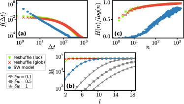
Figure 4: Correlations among concepts produced by an ERRW ($\delta w=0.01$) on a SW network ($p=0.02$). (a) Frequency distribution of interevent times $\Delta t$ between consecutive occurrences of the same concept (node in our model). (b) Number $M_{l}$ of different subsequences of length $l$ as a function of $l$. (c) Normalized entropy of the sequence of visited nodes as a function of $n$, the number of times the nodes have been visited. In each panel, blue circles show average values over 20 different realizations, while triangles and crosses refer to those of (globally and locally) reshuffled sequences.

To better characterize the correlations, we studied how homogeneously concepts occur in the sequence $\mathcal{S}$, after their first appearance. Following Tria et al. Tria et al. (2014), we have divided the sequence $\mathcal{S}$ in $n^{(A)}$ subsequences of the same length, with $n^{(A)}$ being the total number of occurrence of $A$ in $\mathcal{S}$, and we have evaluated the Shannon entropy Shannon (2001) $H^{(A)}=-\sum_{s=1}^{n^{(A)}}p^{(A)}_{s}\log p^{(A)}_{s}$ for every concept $A$, where $p^{(A)}_{s}=n^{(A)}_{s}/n^{(A)}$ denotes the probability of finding concept $A$ in subsequence $s$. Figure 4(c) shows the normalized average entropy $H(n)$ of concepts appearing $n$ times. Again, the large differences with respect to the null models reveal the correlated dynamics of our model. Similar results are obtained for the network of relationships among scientific concepts SuppMat , confirming the validity of the choice of SW networks as underlying structures.

In summary, the mechanism of coevolution of network and random walks introduced in this work naturally reproduces all the properties observed in real innovation processes, including the correlated nature of exploration trajectories. With the topology of the network being a key ingredient of the model, we hope our framework will be found useful in all cases where the network can be directly reconstructed from data, as in the study of scientific innovations reported here.

Supplemental material: Network dynamics of innovation processes

I NULL MODELS: reshuffling the sequences

In the main text, in order to check whether the sequences produced by our ERRW model are correlated, we have compare them to reshuffled versions of the sequences. More precisely, given a trajectory $\mathcal{S}$ of visited nodes (concepts), it is possible to define two null models based on the following two reshuffling procedures Tria et al. (2014). The simplest procedure consists in the global reshuffling of all the elements of $\mathcal{S}$ (indicated as glob in Figure 4 of the main text). This method destroys indeed the correlations (if there are any) in the sequence, but it also modifies the rate at which the new concepts appear, ultimately changing the exponent of the Heaps’ law. Contrarily, the rate can be preserved by defining a second version of the null model, based on a local reshuffling (indicated as loc in Figure 4 of the main text). In this second procedure we reshuffle all the elements in $\mathcal{S}$ only after their first appearance, such that a concept cannot be randomly replaced in the sequence before the actual time it has been discovered.

II CORRELATIONS produced by ERRWs on real networks

In the main text, we have shown how the ERRW model on small-world (SW) networks is able to produce correlated sequences of concepts. We have also proposed a study case of the ERRW model on real topologies extracted from empirical data. In particular, we have explored the cognitive growth of science by extracting empirical sequences of relevant concepts in different scientific fields. For each of the fields considered, we have then tuned the reinforcement parameter of our model in order to produce sequences with the same Heaps’ exponents as the empirical ones (see Figure 3 and Table 1 of the main text). Here, we investigate correlations in the sequences produced by ERRWs on real networks. Figure S1 reports the same quantities we used to study correlations in sequences produced by ERRW on synthetic small-world networks (see Figure 4 of the main text), namely the average entropy of the sequence (Figure S1(a)), number $M_{l}$ of different subsequences of length $l$ as a function of $l$ (Figure S1(b)), and frequency distribution $f(\Delta t)$ of inter-event times $\Delta t$ between couples of consecutive concepts (Figure S1(c)). In each plot, results are compared to the two null models defined in Section I of this Supplemental Material, confirming the correlated nature of the sequences. Furthermore, the comparison with the same statistics obtained for ERRWs on SW networks (see Figure 4 of the main text) confirms again that small-world topologies represent a good choice for modeling the relations among concepts.

III CORRELATIONS produced by ERRWs on synthetic networks

In the main text we have implemented the ERRW model on small-world networks, which proved to be good topologies for modeling the structure of relations among concepts (see Section II of this text and Refs Gravino et al. (2012); Motter et al. (2002); Benedek et al. (2017)). In addition to the plots in Figure 4 of the main text, where we studied the correlations produced by an edge-reinforced random walk over a SW network with fixed link probability $p$ for a fixed amount of reinforcement at $\delta w=0.01$, here we show the curves of average entropy of sequence (Figure S2) and frequency distribution $f(\Delta t)$ of inter-event times $\Delta t$ between couples of consecutive concepts (Figure S3) for different values of reinforcement, ranging from $\delta w=0.001$ to $\delta w=1$. Three different cases of SW networks with $N=10^{6}$ nodes and respectively with link rewiring probability $p=0.001$ (Fig. S2(a-d) and Fig. S3(a-d)), $p=0.01$ (Fig. S2(e-h) and Fig. S3(e-h)) and $p=0.1$ (Fig. S2(i-l) and Fig. S3(i-l)), are considered. All the curves are compared to the corresponding null models as defined in Section I of this Supplemental Material.

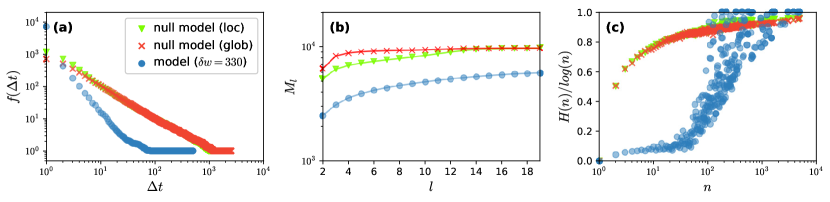
Figure S1: Correlations among concepts for the growth of knowledge in science (Astronomy shown) produced by an ERRW model. The ERRW is tuned to the empirical data by selecting the reinforcement $\delta w$ that reproduces the Heaps’ exponent $\beta$ obtained by fitting the associated Heaps’ curve as a power law (for the Astronomy case shown $\delta w=330$). (a) Frequency distribution of inter-event times $\Delta t$ between consecutive occurrences of the same concept (node in our model). (b) Number $M_{l}$ of different subsequences of length $l$ as a function of $l$. (c) Normalized entropy of the sequence of visited nodes as a function of $n$, the number of times the nodes have been visited (see the main text for details). In each panel, blue circles show average values over 20 different realizations, while triangles and crosses refer to those of (globally and locally) reshuffled sequences.

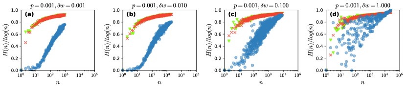
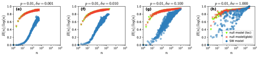
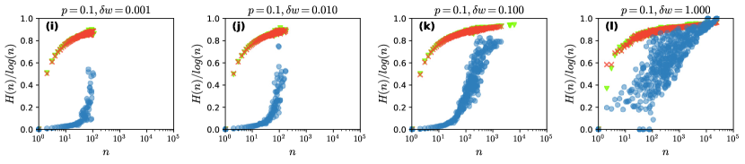
Figure S2: Correlations among concepts produced by an edge-reinforced random walk on a SW network for different values of link probability $p$ and reinforcement $\delta w$ (see the main text for details). Normalized entropy of the sequence of visited nodes as a function of $n$, the number of times the nodes have been visited. In each panel, blue circles show average values over 20 different realizations, while triangles and crosses refer to those of (globally and locally) reshuffled sequences.

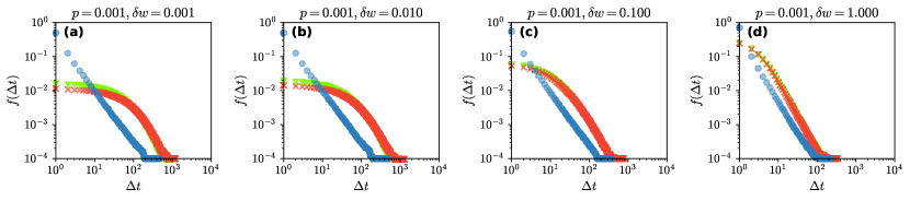
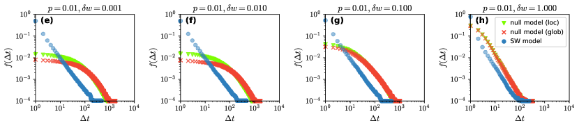
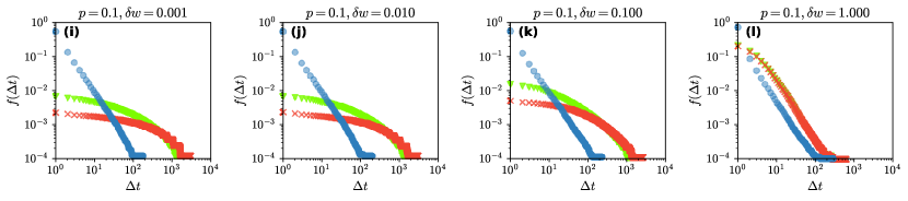
Figure S3: Correlations among concepts produced by an edge-reinforced random walk on a SW network for different values of link probability $p$ and reinforcement $\delta w$ (see the main text for details). Frequency distribution of inter-event times $\Delta t$ between consecutive occurrences of the same concept (node in our model). In each panel, blue circles show average values over 20 different realizations, while triangles and crosses refer to those of (globally and locally) reshuffled sequences.

IV The effect of the average degree on the reinforcement

To better understand the wide range of values obtained for the reinforcement parameter from the analysis of the growth of knowledge in different scientific fields (see Table 1 of the main text), we looked at the relation between the exponent $\beta$ extracted from the Heaps’ law and the reinforcement $\delta w$ in networks with different average node degree. Figure S4 shows $\delta w$ versus $\beta$. Each curve corresponds to Erdős-Rényi random graphs with $N=10^{5}$ nodes and average degrees $\langle k\rangle$ ranging from 6 to 80. As expected, the average degree significantly impacts the reinforcement. In particular, the higher the value of $\langle k\rangle$, the stronger the reinforcement $\delta w$ has to be in order to produce the same Heaps’ exponent. This is easily understandable if one considers the possible choices of a walker reaching a node connected to a link that has been reinforced. If the node has a high degree, the probability of selecting that specific link among all the others will be smaller, and the walker will more easily select a new link, leading to a previously undiscovered node, and therefore to a higher $\beta$. If one wants to keep a certain discovery rate in networks with higher $\langle k\rangle$, higher values of reinforcement will then need to be considered.

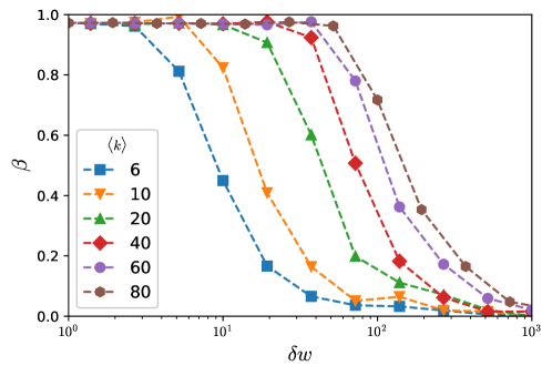
Figure S4: ERRW on ER networks with $N=10^{5}$ and average degree $\langle k\rangle$. Heaps’ exponent $\beta$ as a function of reinforcement $\delta w$.

V Comparing ERRWs to the network version of the urn models

Here we clarify some aspects regarding similarities and differences between our ERRW model and the urn models proposed by Tria et al. Tria et al. (2014), together with their network versions.
In the main text, we state that for the edge-reinforced random walk (ERRW) model, the conditional probability $\text{Prob}\left[X_{t+1}=i|i_{0},i_{1},\ldots,i_{t}\right]$ that, at time step $t+1$, the walker is at node $i$, after a trajectory $\mathcal{S}=(i_{0},i_{1},i_{2},\ldots,i_{t})$, depends on the whole history of the visited nodes, namely on the frequency but also on the precise order in which they have been visited. This is different from what happens in the basic version of the urn model. Using the notation introduced by Tria et al. Tria et al. (2014), in the main text, by urn model (UM) we referred to the basic urn model, i.e. the urn model without semantic. In this case, each ball in the urn has the same probability of being extracted. Since there might be multiple balls of the same color, the probability to extract a given color will depend on the number of balls of that color, and also on the total number of balls in the urn. The number of balls of a given color at time $t$ depends on how many times balls of that color have been extracted up to time $t$ (i.e. on how many times the color has been reinforced), but it does not depend on the specific order of appearance in the sequence of extracted balls. The number of balls in the urn at time $t$ depends on the number of balls initially present in the urn, plus the ones added by mean of the reinforcement mechanism ($\rho$ additional balls for every $t$), plus the balls representing the “adjacent possible” ($\nu+1$ additional balls, every time a color is extracted for the first time).

For example, let us consider the UM with parameters $\rho=1$ and $\nu=0$, and let us indicate as $R$, $B$, $G$ balls respectively of color Red, Blue and Green. By $\mathcal{U}_{t}$ we indicate the urn at time $t$, while $\mathcal{S}_{t}$ represents the sequence of extracted colors from the urn at time $t$, which will trigger a reinforcement at $t+1$ of $\rho=1$ new balls of color $X$ every time a ball of color $X$ is extracted, and a further addition of $\nu+1=1$ balls of new colors every time a color is extracted for the first time (novelty).

A possible evolution, starting from an initial condition with one red ball in the urn at time $t=1$, is the following:

At $t=1$, $\mathcal{U}_{1}=\{R\}$. A $R$ ball is drawn: $\mathcal{S}_{1}=(R)$. $R$ is reinforced and $B$ is added to the urn.
At $t=2$, $\mathcal{U}_{2}=\{R,R,B\}$. A $B$ ball is drawn: $\mathcal{S}_{2}=(R,B)$. $B$ is reinforced and $G$ is added;
At $t=3$, $\mathcal{U}_{3}=\{R,R,B,B,G\}$. A $R$ ball is drawn: $\mathcal{S}_{3}=(R,B,R)$. $R$ is reinforced;
At $t=4$, $\mathcal{U}_{4}=\{R,R,R,B,B,G\}$. A $R$ ball is drawn: $\mathcal{S}_{4}=(R,B,R,R)$. $R$ is reinforced;
At $t=5$, $\mathcal{U}_{5}=\{R,R,R,R,B,B,G\}$. A $B$ ball is drawn: $\mathcal{S}_{5}=(R,B,R,R,B)$. $B$ is reinforced;
At $t=6$, $\mathcal{U}_{6}=\{R,R,R,R,B,B,B,G\}$.

Now, the probabilities of extracting balls of different colors at time $t=6$ are respectively: $p_{R}=1/2,p_{B}=3/8$ and $p_{G}=1/8$.

Notice that another possible evolution, starting from the same initial condition, is the following:

At $t=1$, $\hat{\mathcal{U}}_{1}=\{R\}$. A $R$ ball is drawn: $\hat{\mathcal{S}}_{1}=(R)$. $R$ is reinforced and $B$ is added to the urn.
At $t=2$, $\hat{\mathcal{U}}_{2}=\{R,R,B\}$. A $R$ ball is drawn: $\hat{\mathcal{S}}_{2}=(R,R)$. $R$ is reinforced;
At $t=3$, $\hat{\mathcal{U}}_{3}=\{R,R,R,B\}$. A $B$ ball is drawn: $\hat{\mathcal{S}}_{3}=(R,R,B)$. $B$ is reinforced and $G$ is added;
At $t=4$, $\hat{\mathcal{U}}_{4}=\{R,R,R,B,B,G\}$. A $B$ ball is drawn: $\hat{\mathcal{S}}_{4}=(R,R,B,B)$. $B$ is reinforced;
At $t=5$, $\hat{\mathcal{U}}_{5}=\{R,R,R,B,B,B,G\}$. A $R$ ball is drawn: $\hat{\mathcal{S}}_{5}=(R,R,B,B,R)$. $R$ is reinforced;
At $t=6$, $\hat{\mathcal{U}}_{6}=\{R,R,R,R,B,B,B,G\}$.

Although the two sequences generated at time $t=5$ are different, namely $\hat{\mathcal{S}}_{5}\neq\mathcal{S}_{5}$, they contain the same number of entries for each color, and the two urns at time $t=6$ will be equal, namely $\hat{\mathcal{U}}_{6}=\mathcal{U}_{6}$, so that the probabilities of extracting balls of different colors at time $t=6$ will be $p_{R}=1/2,p_{B}=3/8$ and $p_{G}=1/8$ also for the second urn evolution.

With this simple example we have been able to show that the probability of extracting a color at a given time depends on the number of balls of each color, but not on the precise order of the extracted balls.

Our focus until now has been on the basic UM proposed by Tria et al. There is however a more refined version of the model proposed in Ref. Tria et al. (2014), called urn model with semantic triggering, from now on UMS. In this second version, the authors propose an urn model that is also able to reproduce the correlations of empirical sequences. The model is based on the introduction of semantic labels attached to the balls (different balls and colors might share the same label), together with a mechanism named semantic triggering. The semantic triggering mechanism is able to produce correlated sequences, but it also requires the addition of a third parameter, namely $\eta$, to the model. Notice, instead, that the model we propose in this paper does not need labels or additional mechanisms. In our model correlations emerge naturally from the co-evolution of the walker dynamics and the network.

Finally, in the Supplementary Information of Ref. Tria et al. (2014) the authors discuss how to map urn models into a growing network framework. Such a mapping is exact only in the case when $\eta=1$, which actually corresponds to the simple UM without semantic and thus without correlations. Contrarily, when $\eta\leq 1$, i.e. in the case of the UMS in which the model is able to produce correlated sequences, the mapping is not one-to-one. The key difference is in fact that in a network the connections are always well defined (a link exists or not). In fact, the possibility of going from a node $n_{A}$ to any other node is restricted to the neighbors of $n_{A}$, while for the case of the urn model the possibility of drawing any ball $X$ after the extraction of a given ball $A$ is always probabilistic. As a consequence, the network framework of the urn model presented in S.I. of Ref. Tria et al. (2014) works exactly only for the very specific case $\eta=1$ corresponding to a fully connected network (where a walker can move from each node to every other node, in the same way as any ball can be drawn from an urn after the extraction of any other ball).