dune-composites – A New Framework for High-Performance Finite Element Modelling of Laminates

Abstract

Finite element (FE) analysis has the potential to offset much of the expensive experimental testing currently required to certify aerospace laminates. However, large numbers of degrees of freedom are necessary to model entire aircraft components whilst accurately resolving micro-scale defects. The new module dune-composites, implemented within DUNE by the authors, provides a tool to efficiently solve large-scale problems using novel iterative solvers. The key innovation is a preconditioner that guarantees a constant number of iterations regardless of the problem size. Its robustness has been shown rigorously in Spillane et al. (Numer. Math. 126, 2014) for isotropic problems. For anisotropic problems in composites it is verified numerically for the first time in this paper. The parallel implementation in DUNE scales almost optimally over thousands of cores. To demonstrate this, we present an original numerical study, varying the shape of a localised wrinkle and the effect this has on the strength of a curved laminate. This requires a high-fidelity mesh containing at least four layers of quadratic elements across each ply and interface layer, underlining the need for dune-composites, which can achieve run times of just over 2 minutes on 2048 cores for realistic composites problems with 173 million degrees of freedom.

1 Introduction

Traditionally, aerospace structures have been largely manufactured by subtractive processes, such as machining, which is typically applied to metals. Composite materials, which constitute over 50% of recent aircraft construction, are created at the same time as the structure itself; typically by an additive layup process such as automated fibre placement (AFP). This co-assembly of material and structure is achieved by sequential deposition of a number of fibrous layers which are either pre-impregnated or post-infused with resin, involving hundreds of additive operations during the production of a large structural part. Most of these processes take place before the resin is cured, when the influence of temperature and pressure on the deposition, forming and curing of parts with complex geometry is not well understood. For this reason production is vulnerable to defects arising from small process variations and achieving high-rate automation of the process is limited.

The ability to manufacture composite material-structural systems with repeatable properties at a reasonable rate and competitive cost, with the quality required for certification, is a major challenge in the global aerospace industry. A number of defect types can arise, and use of non-destructive evaluation is limited in detecting these, hence conservative ‘knock-down’ factors are applied to strength limits. These factors are currently obtained by expensive testing at all scales in the Test Pyramid, with large numbers of small coupon tests and fewer larger-scale structural tests. Large-scale tests, are extremely expensive and take place at a stage when it is difficult to make changes and improve designs, while small-scale coupons do not represent the performance of the material at the structural scale where, for example, defects can be introduced as a result of complex forming processes. Furthermore, the boundary conditions and loading in a simple element are very different from the performance of the material within the structure.

One loading of particular interest is corner unfolding, in which though thickness tensile loading acts to separate the layers as the corner radius is increased under bending loads. These stresses act in the weak resin-dominated direction of the laminate and can therefore lead to a limiting design case. The presence of defects such as mis-aligned fibres in the form of out-of-arc wrinkles can have a significant importance. Such a reduction in strength is referred to in manufacturing as a knock-down factor.

Mukhopadhyay et al have modelled the effect of defects on compressive [22] and tensile [23] strength in flat laminates using 8-node, solid elements and zero-thickness, 8-node, cohesive elements between plies. Damage modelling accounted for nonlinear shear in plies, transverse matrix cracking, mixed mode delamination, tensile fibre fracture and fibre kinking. The minimum size of the FE mesh was one ply thickness (0.25 mm) in the vicinity of wrinkles and towards laminate edges. The compressive strength predictions were in agreement to within 10% of experimental results and were able to pick up a mode switch from fibre failure to delamination when defect misalignment was above $\sim 9^{\circ}$. In the tensile case, it was noted that wrinkles act as local, through-thickness shear stress concentrators. For multidirectional laminates, the influence of the defect was exacerbated by edge effects.

We have previously shown that the application of a $3$ mm tough resin layer to the longitudinal edges of corner unfolding specimens prevents the zero stress requirement along the edge, thus reducing the numerical singularity at the edge. The finite element solution becomes more realistic for a given mesh fidelity and failure prediction methods become more accurate. Such an edge treatment can increase the strength by up to $20\%$ [14] and provides a more accurate representation of a long structural part.

There is a wide range of defects that can form in composite laminates and a detailed taxonomy of these is presented in [24]. In this paper we evaluate wrinkle defects, which are more likely to form in curved laminates as a result of consolidation onto a male tool [10]. They are also likely to form in curved laminates with tapered sections, which causes double curvature and makes AFP deposition challenging. These wrinkles are important to the performance of curved laminates.

In this paper we present a new FE analysis tool dune-composites for efficient, high-fidelity modeling of laminated composite parts. We show, using a simple test case that the results of dune-composites match up well with the commercial software package ABAQUS in all six stresses. For large scale problems, dune-composites crucially relies on robust iterative solvers for the resulting FE systems. To this end, we introduce the preconditioner GenEO [26, 27, 19], which we have implemented within DUNE. This preconditioner has previously been mathematically proven to be robust for isotropic FE systems. We show that these results extend to anisotropic problems and that the solver is suitable for solving large composites problems. Further, we demonstrate its parallel efficiency and its ability to scale to thousands of compute cores, allowing the solution of the large problems with defects mentioned above. We test this module by modeling the unfolding of a curved laminate part containing manufacturing defects, for which a micron scale mesh is needed to accurately compute stresses. We show that dune-composites is able to accurately predict damage initiation and that it does so at a fraction of the computational cost required by ABAQUS.

2 Modelling approach

In this section, we introduce the new high performance finite element module dune-composites, and demonstrate its capability of efficiently and robustly tackling large-scale simulations of composite structures. In the example simulations presented, the composite strength of pristine and defected corner radii are accurately predicted. The analysis assumes standard anisotropic 3D linear elasticity and the failure is assessed using a quadratic damage onset criterion for the initiation of delamination in [8]. This allows the results to be benchmarked against existing numerical results and experiments, given in Fletcher et al. [14]. For this case, the numerical results of this linear model show good agreement with experimental data.

The failure of curved laminates subjected to corner unfolding has been shown to be highly unstable with instantaneous propagation following initiation [14]. Therefore we focus on capturing the initiation of failure accurately by using a high-fidelity 3D mesh, with $4$ or more elements through the thickness of each ply and interface layer. Such an approach has been shown to give accurate results for simple flat coupons [13] and 2D models of a few plies [16]. However, this level of fidelity is typically dropped when modelling larger, more complex parts, such as 3D curved laminates, due to computational limitations. Here, we do not use any of these more complex models in order to reduce the computational requirements.

More complex modelling approaches have been proposed for modelling of defects in the literature, these include the use of composite shell elements [23, 22], interface/cohesive elements [18, 20] and higher-order continuum models [21]. In particular, cohesive elements are commonly used to capture propagation [18], but propagation is considered less important than initiation for the problem. The formulation of such elements, whilst more complex, is possible within dune-composites. The solution strategy would require Newton iterations and path-following methods (available in the DUNE library). However, even for these non-linear models of failure, computational cost is still dominated by the speed of solving a linearised system of equations for composite materials. In this paper our focus is therefore on developing and implementing an efficient solution strategy for these linearised equations arising from such massive composite simulation.

2.1 dune-composites: High performance FE modelling of large-scale composite structures

DUNE (Distributed and Unified Numerics Environment) is an open source modular toolbox for solving partial differential equations (PDEs) with grid-based methods, such as the finite element method (FEM) [4, 5, 6]. Written using modern C++ programming techniques, the core modules of DUNE have been developed by mathematicians and computer scientists to allow users to implement and use state-of-the-art mathematical methods across large high performance parallel computing architectures. It is a generic package that provides a user with the key ingredients for solving any FEM problem, e.g. grid generation, different types of finite elements, quadrature rules and a choice of off-the shelf solvers.

Within this platform, we have developed a new module, dune-composites, which solves the linear elasticity equations with general, anisotropic stiffness tensor, applicable for modelling composite structures. This module provides an interfaces to handle composite applications which includes stacking sequences, complex part geometries and complex boundary conditions such as multi-point constraints, or periodic boundary conditions. Further, we have implemented a new $20$-node 3D serendipity element (with full integration) within dune-pdelab, which is not prone to shear locking and allows comparison with ABAQUS’s C3D20R element. This element has degrees of freedom at the $8$ nodes of the element as well as on each of the $12$ edges.

The main advantage of implementing our simulation tool within DUNE is that it allows us to exploit developments in state of the art solvers such as Algebraic Multigrid (AMG), see [3], or to implement new ones. In particular, as part of our new developments, we implemented a novel, robust preconditioner, called GenEO [27, 26], within DUNE. Finally, we will show in Section 2.4 that DUNE allows for highly parallelised efficiency on hundreds of computer cores. This allows for the modelling of meshes fine enough to resolve defects or the modelling of wide parts with sufficient accuracy.

2.2 Verification of DUNE

In this section we show that DUNE produces stress results that are comparable to those produced by standard FE libraries such as ABAQUS. For our comparison we examine a corner unfolding test in DUNE and ABAQUS and compare the solutions as well as the run times. We initially use a small computationally inexpensive problem for comparisons with ABAQUS and move to a larger problem to demonstrate the parallel efficiency of DUNE.

Figure 1 shows the setup of our problem. For this small test we use a width $W=$ 15mm and $L=$ 3mm long limbs. The inner radius $R$ of the curved section is 6.6mm. The overall thickness $T$ is 2.98mm, where the ply layers are 0.23 mm thick and the resin interfaces are 0.02 mm thick. We then apply a resin treatment of 2mm to the free edges of the laminate. This type of edge treatment has been shown in [14] to be advantageous both for reducing conservatism in the design of aircraft structures, as well as to make FE analyses more reliable. The mechanical properties for the ply material and for the resin interfaces of the curved laminate are given in Table 1. The fibre angles are given by the following $12$-ply stacking sequence

$$\left[\pm 45/90/0/\mp 45/\mp 45/0/90/\pm 45\right].$$

Orthotropic fibrous layer		Isotropic interface layer
$E_{11}$	162 GPa	$E$	10 GPa
$E_{22},\,E_{33}$	10 GPa	$\nu$	0.35
$G_{12},\,G_{13}$	5.2 GPa
$G_{23}$	3.5 GPa	Resin edge material
$\nu_{12},\,\nu_{13}$	0.35	$E$	8.5 GPa
$\nu_{23}$	0.5	$\nu$	0.35

Table 1: Mechanical properties for the curved $12$-ply laminate.

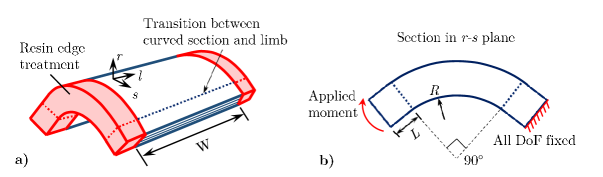
Figure 1: Sketch of the edge-treated corner-unfolding specimen (left) and a cross section of the configuration (right).

In ABAQUS, the corner unfolding is modelled using a beam-type multi-point constraint (MPC) at the end of one limb. In DUNE, a similar effect is achieved by adding a thin layer of very stiff material at the end of the same limb. In both cases, a $96.8$ Nmm/mm moment is applied to that limb, while fixing all degrees of freedom on the other limb, as shown in Figure 1. We denote the stresses using the following directional notation: arc length $s$ (around the curve); radius $r$ through-thickness and width $l$ across the laminate. These are shown by the coordinate system in Figure 1a.

DUNE and ABAQUS both use a model with second-order serendipity elements (element C3D20R in ABAQUS, [1]). There is a small difference in that ABAQUS uses reduced integration while DUNE uses full integration. Also, the stresses are not recovered in an identical way from the displacements in the two codes. We use a tensor-product grid with $56$ elements in the $l$ and $s$ directions and $6$ elements in each of the 12 fibrous and the 11 interface layers in the $r$ direction. In total, this mesh contains $432,768$ elements. To ensure the effects at the free edge and at the material discontinuities are sufficiently resolved, the FE mesh is graded towards both edges in the $l$ direction, as well as towards the interfaces in each of the resin and fibrous layers in the $r$ direction. The bias ratio gives the ratio between width of the smallest and largest element of the mesh. We choose a bias ratio of $400$ between the centre and the edges of the structure in the $l$ direction and a bias ratio of $10$ between the centre and the interfaces in each layer in the $r$ direction.

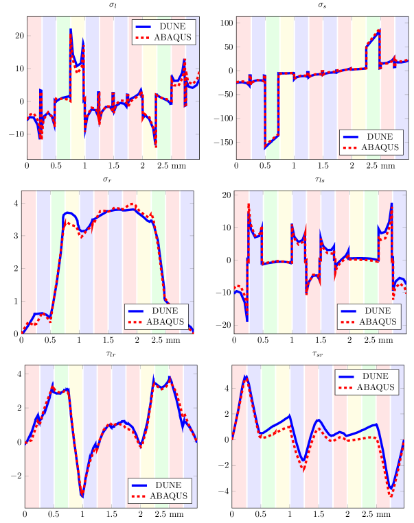
Figure 2: Stresses in MPa as a function of radius $r$ from outer radius at the apex of the curve, at $2.156$mm from the edge of the resin-edge-treated laminate (DUNE, solid blue; ABAQUS, dotted red). The background colours indicate the stacking sequence: $+45$ = red, $-45$ = blue, $90$ = green, $0$ = yellow.

In Figure 2, all six stresses computed with ABAQUS and DUNE are compared at the apex of the curve (i.e., at an angle of $45^{\circ}$) near the resin edge, $2.156$mm away from the edge, which is in the laminate $0.156$mm ($6$ elements) away from the resin laminate edge. Since we use identical meshes and identical elements, the numbers of degrees of freedom are also the same. However, there are some differences in the models, such as the quadrature order, use of single precision in ABAQUS and the stress reconstruction, which could account for the different results. Nevertheless, the results show reasonably good agreement for all six different stresses.

2.3 Efficiency of dune-composites: Robust iterative solvers

The computational gains of dune-composites demonstrated in this section are a direct consequence of the use of fast and robust iterative solvers for the resulting large systems of linear equations

$$K\underline{u}=\underline{f},$$ (1)

where $K$ is the global stiffness matrix, $\underline{f}$ is the load vector arising from the applied boundary conditions and $\underline{u}$ is the solution vector containing the displacement values at each node within the finite element mesh. There are also some significant gains in the setup time due to a more efficient, problem-adapted data management.

Solvers for systems of linear algebraic equations can broadly be classified into direct and iterative ones. Direct solvers, based on matrix factorisation, are more universally applicable and more robust to ill-conditioning [12]. Thus, they are typically the default in commercial FE packages. However, the cost of the factorisation and the memory requirements can quickly become infeasibly high for large problems. Moreover, it is difficult to achieve good parallel efficiencies on large multicore computer architectures. Since they do not require any factorisations, iterative methods for (1) have the potential to scale optimally, both with respect to problem size and with respect to the number of processors in a parallel implementation, but that crucially depends on the ’conditioning’ of the problem.

In size, we refer to the total number of degrees of freedom $N$ in the underlying finite element (FE) solution $\underline{u}$. Below we will see examples, for which $N$ can be very large, up to 60 million. It is important to note that $K$ is sparse, that is, the number of nonzero entries in $K$ is proportional to $N$, which is significantly less than the possible $N^{2}$ entries in a full matrix. Iterative methods only require the storage of the original, sparse stiffness matrix, while the storage of the factors in direct methods is closer to the $N^{2}$ entries in a full matrix. The computational cost of the best direct methods for FE systems arising from three-dimensional structural calculations, such as those used in ABAQUS, still grows at least with order $N^{1.5}$, as we will see below. Iterative solvers that only require multiplication with the sparse matrix $K$ have the potential to scale linearly with the problem size $N$.

The conditioning is a property of the global stiffness matrix $K$. We say that $K$ is ill-conditioned, if the nodal displacements $\underline{u}$ are highly sensitive to rounding errors and to small changes in $\underline{f}$. Generally, simulations of composite structures are ill-conditioned because of the strong heterogeneity and the often complex, non-grid aligned anisotropy of the material. The condition number of $K$, which is defined as the ratio of the largest and the smallest eigenvalue of $K$, grows roughly linearly with the size of the largest jump in the entries of the stiffness tensor from one finite element to an adjacent one. But the conditioning also worsens systematically, as the problem size $N$ increases. This growth is typically of order $N^{2/3}$ in 3D problems. This growth affects the accuracy of the solution in direct solvers, but it has no effect on the computational cost.

By contrast, for iterative methods, such as Gauss-Seidel, conjugate gradients or GMRES methods, the conditioning of $K$ has a direct impact on the number of iterations and thus on the cost. The basic idea of iterative methods is to approximate the solution iteratively, starting from some initial guess, by sequentially reducing the residual

$$r=K\underline{u}-\underline{f}$$

at each iteration [17]. A ’good’ or fast iterative solver reduces this error quickly, in a few iterations. For well-conditioned problems, standard black-box iterative solvers (as offered by ABAQUS) work well. But the number of iterations typically grows with the square-root of the condition number of $K$. For the poorly conditioned problems of interest in this paper, standard iterative methods will either converge very slowly or completely fail to do so.

A standard approach to improve the conditioning of such problems is to apply a preconditioner $P$ to (1), typically a cheap approximation of $K^{-1}$, and then to iteratively solve

$$PK\underline{u}=P\underline{f}.$$ (2)

The better the approximation $P\approx K^{-1}$, the closer the system matrix in (2) is to the identity and thus to a well-conditioned problem with condition number close to $1$. However, as outlined above, computing the inverse of $K$ (e.g. via factorisation) is too expensive. Ideally the cost of applying $P$ and the memory requirements should again only grow linearly with $N$. A good choice of $P$ is problem dependent, and must be carefully designed and tuned, to obtain fast solvers which scale well for large problems over multiple cores. However, some well-understood common design choices for FE discretisations of elliptic partial differential equations exist. To achieve independence (or at most logarithmic dependence) of the number of iterations on the problem size $N$, it is paramount to apply multilevel preconditioners, either in the form of multigrid [7, 29] or multilevel domain decomposition methods [28]. In addition, the memory demands of such iterative solvers are small (proportional to $N$) and the work can be easily distributed over multiple cores.

Care has to be taken though to achieve robustness with respect to heterogeneities and anisotropies in the material properties. Since black-box multilevel approaches do not scale indefinitely and are not robust, more tailor-made approaches are needed. The flexibility to prescribe or implement such tailor-made preconditioners is not available in commercial software, and therefore the development of codes like dune-composites is pivotal in solving large-scale problems in composite structures.

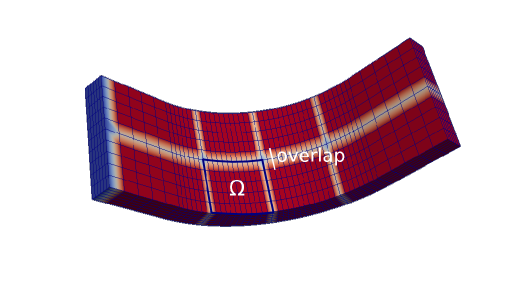
Figure 3: Decomposition of a mesh into several subdomains ($\Omega$), showing an overlap of one element in each subdomain.

In dune-composites we use the conjugate gradient (CG) iterative method for (2) and we test two types of preconditioner: the generic Algebraic Multi Grid (AMG) preconditioner [3], as well as a new two-level overlapping domain decomposition preconditioner (GenEO) with a multiscale coarse space based on local, generalised eigensolves in each of the subdomains [27]. For their parallelisation, both methods partition the physical domain and the FE mesh into subdomains of roughly equal size and distribute them across multiple cores (see Figure 3). The key ingredient in both preconditioners is a coarse approximation of $\underline{u}$ with significantly fewer degrees of freedom that is cheaper to obtain then $\underline{u}$. This coarse approximation is then interpolated back to the original FE mesh.

In Algebraic Multigrid, the problem is coarsened repeatedly by aggregating degrees of freedom in the stiffness matrix $K$, creating a hierarchy of coarse approximations of decreasing size. The aggregation process is purely algebraic and based on the fact that the displacement $u_{i}$ and $u_{j}$ at two neighbouring nodes $x_{i}$ and $x_{j}$ in the FE mesh will be similar if the nodes are “strongly connected”, i.e. $u_{i}\approx u_{j}$ if $|K_{i,j}|$ is large (relative to $|K_{ii}|$ and $|K_{jj}|$). The degrees of freedom at two (or more) nodes that are strongly connected are then aggregated to a single degree freedom to obtain a cheaper approximation. This process can be applied recursively until a sufficiently coarse approximation has been obtained that can be efficiently solved using a direct method. On the intermediate levels and on the original mesh we only apply a cheap relaxation method such as Gauss-Seidel. The success of the AMG preconditioner largely depends on how well this aggregation process works (for details see [3, 29]).

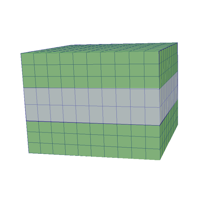
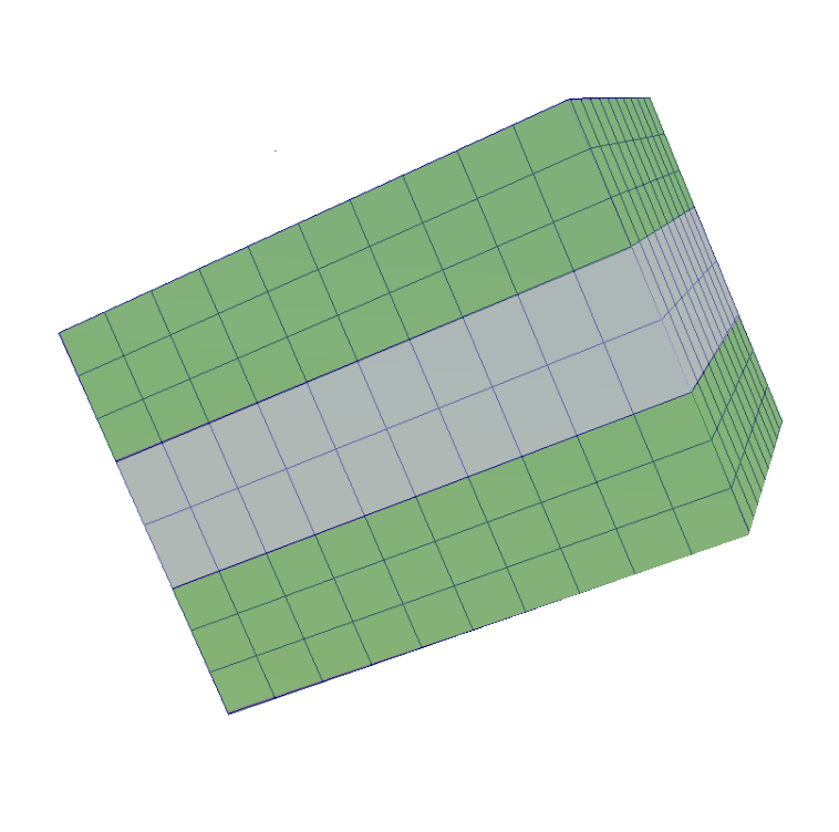
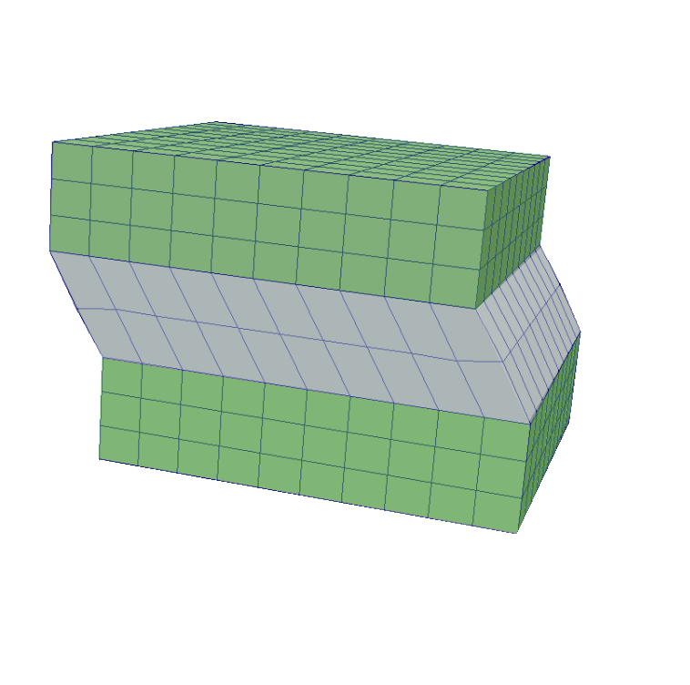
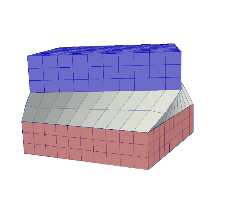
Figure 4: Schematic of low energy eigenmodes in a reference block consisting of a layer of resin (white) between two layers of plies (green: $90^{\circ}$, blue: $-45^{\circ}$, red: $45^{\circ}$); from left to right, a reference block, a zero energy mode (rotation), a low energy mode between two $90^{\circ}$ plies and a low-energy twisting mode caused by $45^{\circ}$ and $-45^{\circ}$ plies.

The GenEO preconditioner is of overlapping Schwarz-type [28] and uses only two levels. The domain is partitioned into overlapping subdomains of roughly equal size (see Figure 3). In each of these subdomains, the original FE problem subject to zero-displacement boundary conditions on the artificial subdomain boundaries is solved either exactly using a direct method or approximately using, for example the AMG preconditioner. To capture the global behaviour of the solution, a coarse problem is introduced. For homogeneous structures, standard finite elements on a coarser mesh are sufficient [28]. For composite structures, especially in the presence of defects, this approach is too inaccurate. Instead, the GenEO preconditioner computes a few of the smallest energy (eigen) modes of the structure on each of the subdomains. This includes the rigid body modes, but also some more exotic modes that arise due to the particular properties of the composite. Some of these low energy modes can be seen in Figure 4. Finally, these local modes are combined to generate a coarse global approximation using a so-called partition of unity approach [28]. The coarse problem is again solved using a direct method or an iterative method. For details see the original paper [27] and the related works [15, 2]. The GenEO coarse space has been shown to lead to a fully robust two-level Schwarz preconditioner which scales well over multiple cores [27, 19]. For isotropic problems this has been proved rigorously in [27]. The robustness is due to its good approximation properties for problems with highly heterogeneous material parameters. This is in fact of independent interest [2, 11]. Details of our specific implementation of GenEO in DUNE are given in [25].

2.4 Performance Tests and Parallel Efficiency

First, we compare the performance of various preconditioners for the iterative solver in dune-composites when simulating the problem specified in Section 2.2, as well as benchmarking them against the direct solver in ABAQUS. The iterative solvers in ABAQUS only converge for homogeneous problems or for very small numbers of degrees of freedom. The measures for comparing the solvers are their overall computational cost and their parallel efficiency. All the experiments in Figure 5 were carried out on the computer cts04 which consists of four 8-core Intel Xeon E5-4627v2 Ivybridge processors, each running at 1.2 GHz and giving a total of 32 available cores.

On the left in Figure 5, we compare the iterative solver with AMG preconditioner in DUNE (with tolerance $10^{-4}$) and the sparse direct solver in ABAQUS for increasing problem sizes. We see that the iterative solver in DUNE scales linearly with the problem size $N$ (the number of degrees of freedom) while the cost of the direct solver in ABAQUS grows significantly faster. Asymptotically, the growth is more than quadratic in $N$. Moreover, the direct solver runs out of memory on one core for the biggest problem tested in DUNE ($N\approx 7.5$ million). We specifically use the block version of AMG in our tests in dune-composites and measure strength of connection between two blocks for the aggregation procedure in the Frobenius norm. As the smoother, we use two iterations of symmetric successive overrelaxation (SSOR). The number of iterations remains almost constant and moderate in this test. However, AMG has not originally been designed for serendipity elements, and in its current form it does not seem to be robust for this element, especially in parallel.

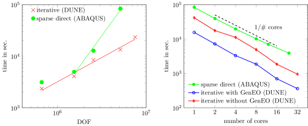
Figure 5: Left: Timing comparison in terms of degrees of freedom between the sparse direct solver in ABAQUS and the iterative CG solver (with AMG preconditioner) in DUNE. Right: Timing comparison in terms of numbers of cores between the sparse direct solver in ABAQUS and the iterative CG solver (with one- and two-level domain decomposition preconditioner) in DUNE.

The second comparison, on the right in Figure 5, shows the parallel scaling of various solvers. Here, we plot the strong scaling, that is, the reduction in computational cost due to an increase in the number of cores for a fixed problem size. We see that up to $32$ cores both the parallel direct solver in ABAQUS (green curve), as well as the iterative solver with domain decomposition preconditioner in DUNE (red and blue curves) show almost optimal parallel scaling, that is, the CPU time is halved every time the number of cores doubles. We tested two versions of the domain decomposition preconditioner. The red line corresponds to a one-level overlapping Schwarz preconditioner with an overlap of two layers of finite elements. The subdomain problems are solved with UMFPACK [9], a sparse direct solver, similar to the one in ABAQUS. For 1-8 cores, we use 8 subdomains and partition them evenly onto the available cores. For 16 and 32 cores, we use 16 and 32 subdomains, respectively (one per core). The blue line corresponds to the new GenEO preconditioner, a two-level overlapping Schwarz preconditioner where, in addition to the subdomain solves, we also build and solve a problem-adapted coarse problem (see Section 2.3) . This coarse problem is again solved using UMFPACK.

The addition of the domain decomposition preconditioner was essential for a good parallel efficiency. For some reasons which we cannot fully explain, the parallel AMG preconditioner, which is available as a default within DUNE did not scale well in parallel. The addition of the GenEO coarse space dramatically reduces the number of iterations from about $400$ for the one-level overlapping Schwarz preconditioner (diamond points) to about $40$ for GenEO (hollow circle). Both those numbers remain roughly constant across this range of cores. In absolute terms, the lower number of iterations for GenEO translates into an almost three-fold reduction in computational time. Moreover, beyond 32 cores, only the GenEO preconditioner continues to scale. The numbers of iterations for the one-level Schwarz preconditioner start to increase with the number of subdomains.

Finally, we note that even for the relatively small test we have chosen here ($432,768$ elements) the iterative solver in DUNE preconditioned with GenEO is around $5-10$ times faster than the direct solver in ABAQUS. Moreover, the restriction to shared-memory parallelism and the memory requirements of the direct solver in ABAQUS, combined with the $O(N^{2})$ growth in computational cost, make it essentially impossible to carry out a corresponding scaling test with ABAQUS beyond $32$ cores.

By contrast, in Figure 6, we now look at the parallel scaling of the iterative solver with GenEO preconditioner in dune-composites on thousands of cores solving problems with up to $173$ million degrees of freedom. We use again UMFPACK for all subdomain and coarse solves in GenEO. For this second scaling test, we move to a larger scale problem. The model run in this section has $39$ plies and a variable width. For details on the setup of this problem see Section 3. We also move to a larger computer. All the experiments in Figure 6 were carried out on the University of Bath HPC cluster Balena. This consists of 192 nodes each with two 8-core Intel Xeon E5-2650v2 Ivybridge processors, each running at 2.6 GHz and giving a total of 3072 available cores.

We carry out a weak scaling experiment, that is, we increase the problem size proportionally to the number of cores used. For an iterative solver that scales optimally both with respect to problem size and with the number of cores, the computational time should remain constant in this experiment. To scale the problem size as the number of cores $N_{\text{cores}}$ grows, we increase the width of the laminate. We present results for two different setups. For the first, larger problem we have used $56$ elements along the radius, $\frac{5}{8}N_{\text{cores}}$ elements across the width and $4$ elements through thickness in each of the resin and ply layers, respectively. This setup ensures that the amount of work handled by each core remains constant as $N_{\text{cores}}$ varies. For the second, smaller problem we have halved the number of elements through the thickness, using only 2 elements in each resin and ply layer. In Figure 6, we see that after a slight initial growth the scaling of the iterative solver in DUNE with GenEO preconditioner is indeed almost optimal to at least $2048$ cores, allowing us to increase the size of the tests at a nearly constant run time and thus, to solve a problem with $173$ million degrees of freedom in just over 2 minutes.

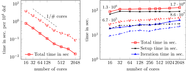
Figure 6: Scaling of dune-composites using the GenEO preconditioner on up to $2048$ cores. Solid lines are used for the problem with $8.4\cdot 10^{4}$ degrees of freedom per core; dashed lines for $4.2\cdot 10^{4}$ degrees of freedom per core. For the larger problem, the problem size varies from about $1.3$ million degrees of freedom on 16 cores to about $173$ million degrees of freedom on 2048 cores.

3 Defect analysis and the influence of boundaries

In manufacturing, small localised defects in the form of misaligned fibrous layers can occur, these defects can have a large effect on the strength of the materials. In this section we investigate the effect that varying the maximum slope and amplitude of a localised wrinkle with only one oscillation has on the strength of the curved laminate. We show that we need a very high-fidelity mesh to be able to compute localised stresses and this problem provides an appropriate application for dune-composites. In order to determine the shape and size of the wrinkle we used an X-ray CT scan of a typical curved laminate with a wrinkle defect, shown in Figure 7 and described in more detail below.

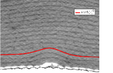
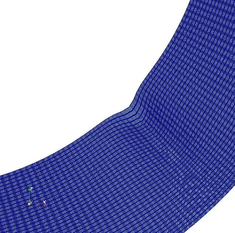
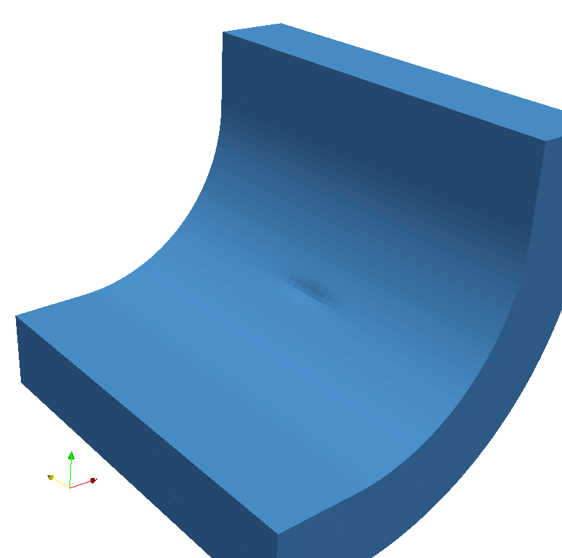
Figure 7: Image of a defect. Left: A scan of a wrinkle with the $\text{sech}^{2}\,(\cdot)$ superimposed. Center: A radial cut through the center of the laminate. Right: Decay of the wrinkle across the width.

For the defect analysis we we examine the influence of width-wise boundary conditions on the results. The mechanical properties for the ply material and the resin interfaces are the same as those for the previous smaller test, see Table 1. The geometry of this $39$ ply problem is chosen to give a similar ratio of width to radius as the previous test. Here we use a width $W$ of 52mm and 10mm long limbs $L$. The inner radius $R$ of the curved section is 22mm. The overall thickness $T$ is 9.93 mm, where the ply layers are 0.24 mm thick and the resin interfaces are 0.015 mm thick. The fibre angles of plies are given by the following stacking sequence

$$\left[[\mp 45/90/0]_{2}/[\mp 45]_{2}/90/\mp 45/90/0/\mp 45/0/\pm 45/0/90/\pm 45/90/[\pm 45]_{2}/[0/90/\pm 45]_{2}\right].$$

Figure 8: Transformation of the flat geometry into a flat geometry with a defect and finally into the curved geometry with a defect.

The boundary conditions and loading in a narrow specimen are very different from those of the full structure. For this reason we initially model using periodic boundary conditions at the free edge. This gives an approximation of the effect of the wrinkle in a very wide part. For the later tests we remove the periodic boundary conditions and add a $3$mm wide layer of resin to the free edges. This reduces the strength of the singularity at this edge and for larger wrinkles, ensures that failure occurs at the center of the laminate, near the defect.

Figure 8 shows the process by which the wrinkle is created. We start with a mesh on a flat plate, then we add the wrinkle to the flat plate and finally transform to the curved geometry. Let $(s,l,r)$ be coordinates in the unperturbed, flat geometry. Note, that in the final curved geometry, $s$ corresponds to an arc length, $r$ is the radius through the part and $l$ is the width across the part.

In the flat geometry the wrinkle is given by a perturbation in $r$, which depends on all three coordinates. The perturbed coordinates $(\hat{s},\hat{r},\hat{l})$ are given by

$$\hat{s}=s,\quad\hat{l}=l\quad\text{and}\quad\hat{r}=r+f(s,l,r).$$ (3)

If we denote by $(s_{\text{def}},l_{\text{def}},r_{\text{def}})$ the location where the defect is largest, the perturbation is given by

$$f(s,l,r)=d\,\text{sech}^{2}\left(\pi\frac{s-s_{\text{def}}}{\pi b_{1}}\right)\,\text{sech}^{2}\left(\pi\frac{r-r_{\text{def}}}{Rb_{2}}\right)\,\text{sech}^{2}\left(\pi\frac{l-l_{\text{def}}}{Wb_{3}}\right),$$ (4)

where $d$ gives the amplitude of the defect and $b_{i}$, $i=1,2,3,$ are parameters giving the “extent” of the defect in the three directions.

For these tests we have chosen $b_{2}$ so that the wrinkle decays more quickly towards the inner radius, more precisely

$$b_{2}=\begin{cases}\frac{1}{2}&\text{ if }r-r_{\text{def}}<0\\ \frac{1}{4}&\text{ if }r-r_{\text{def}}>0\end{cases}.$$

Further, $b_{1}=\frac{1}{5}$ and $b_{3}=\frac{1}{2}$. As shown in Figure 9, the sech${}^{2}(\cdot)$ function never reaches zero, however at $\pm b_{i}$ it is already negligibly small ($<10^{-2}$). The coordinate $s$ ranges from $0$ to $\pi$, $r$ ranges from $R$ to $R+T$ and $l$ ranges from $0$ to $W$, which implies that a value of $b_{3}=\frac{1}{2}$ leads to a wrinkle spanning half of the width of the part.

The wrinkled mesh on the cube is finally mapped to the curved section via the mapping

$$\begin{split}\hat{x}&=g_{1}(\hat{s},\hat{l},\hat{r})=L+\hat{r}\sin\left(\frac{\pi}{2}\hat{s}\right)\\ \hat{y}&=g_{2}(\hat{s},\hat{l},\hat{r})=\hat{l}\\ \hat{z}&=g_{3}(\hat{s},\hat{l},\hat{r})=\hat{r}\cos\left(\frac{\pi}{2}\hat{s}\right),\end{split}$$ (5)

where $L$ is the length of the limb.

From the form of the wrinkle we can easily calculate the steepest slope by deriving

$$\tan^{-1}\left(\frac{d}{ds}f(s,l,r)\right)=\tan^{-1}\left(-\frac{2}{b_{1}}\,\text{tanh}\left(\pi\frac{s-s_{\text{def}}}{\pi b_{1}}\right)f(s,l,r)\right)$$ (6)

This allows us to classify wrinkles according to the steepest angle produced by the defect. In order to ensure that the edge effect does not affect the results we give results with periodic boundary conditions. In Figure 7 we give a sample defect from a CT scan with an overlay showing the fit to our proposed parameterisation of the wrinkle. We also show the resulting model with the largest amplitude (and thus slope) of defect considered in the following numerical tests.

3.1 Convergence Analysis

The FE model used for these tests consists of approximately $7.3\cdot 10^{6}$ degrees of freedom in total. There are $96$ elements along the radius, $40$ across the width and $4$ each in the resin and ply layers. To resolve the defect the model is refined towards the location of the defect, with a bias ratio of $2$, i.e. the elements at the center of the model are half as large as those at the edges. For the edge treated case there is also refinement towards the resin edge with a bias ratio of $400$ to resolve the stress concentrations that occur near the edge.

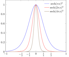
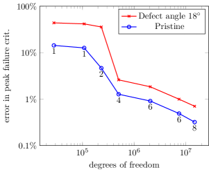
Figure 9: Left: Decay of the sech${}^{2}()$ function for $3$ different values of parameter $B$. Right: Convergence plot for a pristine part and a part with a defect with maximum slope $18^{\circ}$, with labels giving the number of elements through-thickness per ply and interface layer.

To ensure that the FE modelling is sufficiently accurate we include a convergence analysis. In Figure 9 (right) we plot the relative error in the peak failure criterion given by equation (7) below. As an approximation to the exact solution we used the next refinement level of the FE model ($136$ elements along the radius, $60$ across the width and $8$ each in the resin and ply layers). For the refinement we have chosen (second to last point) the relative error has been reduced to around $1\%$ for both the pristine model and for the model containing a defect. For the case with a wrinkle it is important to note that in the first three refinement levels have very similar peak failure criterion, even though the model is not yet converged. However, in these configurations the wrinkle is not yet sufficiently resolved and the failure criterion output is still closer to that of the pristine model.

The models used in this analysis increase the number of elements through thickness in each layer as follows: $1$, $1$, $2$, $4$, $6$, $6$, $8$. The number of elements across the part and around the radius and limbs are increased simultaneously. We can see that (especially for a part with a defect) the number of elements through thickness is very important. With fewer than $4$ elements we do not get a good approximation of the maximum failure criterion. Further, when fewer elements are used the stresses drop to zero at the surface of the laminate.

Around the curve enough elements need to be used to ensure that the wrinkle is resolved, at least $10$ elements should be used along the length of the wrinkle. Even with a mesh grading towards the wrinkle this still requires a large total number of elements across the full length of the part.

3.2 Defect analysis

The stresses in the vicinity of a defect are complex, including interlaminar, shear and direct stresses. Therefore a mixed mode failure criterion is more suitable than a maximum stress criterion. The strength of the laminates was assessed using a quadratic damage onset criterion, defined by Camanho et al. [8] as

$$\sqrt{\left(\frac{\sigma^{+}_{r}}{s_{33}}\right)^{2}+\left(\frac{\tau_{rs}}{s_{13}}\right)^{2}+\left(\frac{\tau_{rl}}{s_{13}}\right)^{2}}=F$$ (7)

with negative values of $\sigma_{r}$ treated as zero and the following allowables:

$s_{33}=$ 61 MPa   $s_{13}=$ 97 MPa.

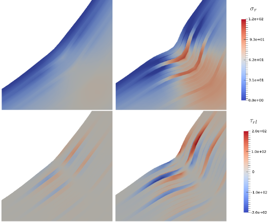
Figure 10: Stresses $\tau_{rl}$ and $\sigma_{l}$ for defect angle $4^{\circ}$ (left) , followed by stresses $\tau_{rl}$ and $\sigma_{l}$ for defect angle $18^{\circ}$ (right).

Curved laminates subjected to corner unfolding are observed to fail by delamination of the plies [14]. Since this indicates failure occurs at the interface between plies, we apply the failure criterion only in the resin-rich interface zones and failure initiates when $F=1$. Generally, the failure criterion is applicable in the local coordinates of the material, however since the interface zone is isotropic, a transformation is not required.

Having established the wrinkle defect model, we now investigate the effect of varying the wrinkle severity. Figure 10 shows the effect on the interlaminar shear and direct stresses with a wrinkle of maximum angle (slope) of $4^{\circ}$ and $18^{\circ}$ for which an opening/bending moment of 9.58 kN mm/mm is applied. The interlaminar shear maximises in the region of greatest slope, while the interlaminar direct stress maximises in the region of peak amplitude. These stresses are highly localised and cause a sharp rise in failure index through-thickness, as shown in Figure 11. The pristine part is predicted to fail near the mid-thickness, where direct interlaminar stress maximises. With a wrinkle of slope $4^{\circ}$, there is a rise in failure index near the inner radius, however failure is still predicted to first occur near the mid-thickness (as per the pristine model). As the slope of the wrinkle is increased, so failure index near the inner radius becomes higher than that near the mid-thickness. This is also indicated in Table 2, showing failure at interface $16$ for pristine and $4^{\circ}$ wrinkle models, and at interface $4$ for greater slopes. For the most severe wrinkle of slope $18^{\circ}$, the failure index is almost double that of the pristine model, and hence strength is halved.

A summary of all models is shown in Table 2. As seen by the maximum recorded displacement, the overall stiffness of the curved laminate is not significantly affected by the inclusion of a wrinkle defect. This is because it is very small in comparison to the size of the whole laminate. However, it does significantly reduce strength, based on initiation of failure. When tested in isolation such specimens have been found to fail in a highly unstable manner, suggesting once initiation is reached there is instantaneous propagation and catastrophic failure [14]. Note that the two pristine results in Table 2 compare well with predictions acquired by modelling the curved laminates using ABAQUS software [14]. Note also that the edge-treated pristine result compares well with experimental results [14]. Table 2 shows that the greatest impact of the wrinkle is to introduce significant interlaminar shear stresses. Interlaminar direct stress is also increased, by approximately $50\%$ between the pristine and $18^{\circ}$ wrinkle models; however, the interlaminar shear stresses go from being negligible in the pristine model, to becoming greater than the interlaminar direct stress in the $18^{\circ}$ model.

Note that these results do not take into account thermal pre-stresses, which occur as a result of the high-temperature curing process and may be significant. However, the purpose of this paper is to illustrate the importance of mesh refinement for rapidly varying through-thickness stresses.

4 Conclusions

In this paper, a new high-performance FE analysis tool for composite structures is presented and shown to accurately model the behaviour of complex laminate structures with manufacturing defects in a fraction of the computational time required by commercial software packages, such as ABAQUS.

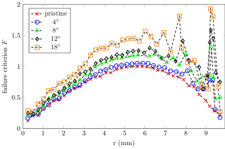
Figure 11: Through-thickness quadratic damage onset criterion $F$ at the center of each resin interface (with linear interpolation between resin interfaces). Values are calculated at mid-width along the angle of steepest slope ($2.1^{\circ}$ from the apex of the curve), and at a distance $r$ from the outer radius.

FEA (normalised): Periodic BC
Defect slope (deg.)	max. disp. (mm)	location	interface (from outer radius)	max. failure crit. $F$	$\sigma_{l}$ (MPa)	$\sigma_{s}$ (MPa)	$\sigma_{r}$ (MPa)	$\tau_{sl}$ (MPa)	$\tau_{rs}$ (MPa)	$\tau_{rl}$ (MPa)	M(kN)
0	3.99	Mid- width	23	1.00	33.76	34.90	61.00	0.19	0.02	$-0.23$	9.581
4	3.98	Mid- width	23	1.07	37.26	40.72	65.59	0.17	0.95	0.47	8.90
8	3.98	Mid- width	35	1.30	51.67	113.2	65.69	$-8.75$	6.50	71.05	7.34
12	3.98	Mid- width	35	1.65	45.41	117.4	79.94	$-12.80$	9.97	97.59	5.78
18	3.98	Mid- width	35	1.94	37.31	131.6	92.99	$-17.37$	14.91	116.4	4.92
FEA (normalised): Resin edge treated
0	5.16	Edge	23	1.16	80.06	116.25	11.13	6.75	28.13	-107.5	8.262
18	5.16	Mid- width	35	1.99	37.68	144.15	96.67	$-16.72$	116.80	0.57	4.79
1 ABAQUS result was $9.51$ kN [14]
2 ABAQUS result was $8.25$ kN, test average $8.65$ kN[14]

Table 2: Effect of the defect angle on peak stresses, on the failure criterion $F$ in interfaces and on M the predicted moment of initiation of failure.

The stress field around a wrinkle defect in composite materials is highly localised, requiring a high fidelity mesh to adequately capture it. Such defects that arise in composite materials during manufacture are by nature difficult to predict. There is a case for performing stochastic analysis: running thousands of simulations with defects in various locations and sizes, studying the influence on the integrity of a component. The high number of simulations, combined with the requirement for high fidelity in each simulation, results in a very demanding problem computationally. The use of a bespoke FE solver, such as the one developed here in DUNE, is essential for meeting these demands.

Current industry standard FE tools, e.g. ABAQUS, are not able to deal with these problem sizes, largely due to the direct linear equation solvers that are employed and the restricted parallel scalability. Iterative solvers within ABAQUS only converge in very simple cases. For this reason, as part of our project, a new iterative solver had to be implemented within DUNE. The heart of this solver is a robust preconditioner (GenEO) that leads to an almost optimal scaling of the computational time both with respect to the number of degrees of freedom and the number of compute cores. This has been demonstrated for problems with up to $173$ million degrees of freedom, achieving run times of just over $2$ minutes on $2048$ cores.

The chosen example problem evaluates the through-thickness stresses caused by unfolding a curved laminate. This serves to illustrate the importance of using high-fidelity meshes and provides insight into the influence of small manufacturing induced defects.

5 Acknowledgements

This work was supported by an EPSRC Maths for Manufacturing grant (EP/K031368/1). Richard Butler holds a Royal Academy of Engineering-GKN Aerospace Research Chair in Composites. This research made use of the Balena High Performance Computing Service at the University of Bath.

References

- [1] D. N. Arnold and G. Awanou. The serendipity family of finite elements. Found. Comput. Math., 11(3):337–344, 2011.
- [2] I. Babuska and R. Lipton. Optimal local approximation spaces for generalized finite element methods with application to multiscale problems. Multiscale Model. Simul., 9(1):373–406, 2011.
- [3] P. Bastian and M. Blatt. On the generic parallelisation of iterative solvers for the finite element method. Int. J. Comput. Sci. Engin., 4:56–69, 2008.
- [4] P. Bastian, M. Blatt, A. Dedner, C. Engwer, R. Klöfkorn, M. Ohlberger, and O. Sander. A generic grid interface for parallel and adaptive scientific computing. Part I: Abstract framework. Computing, 82:103–119, 2008.
- [5] P. Bastian, M. Blatt, A. Dedner, C. Engwer, R. Klöfkorn, M. Ohlberger, and O. Sander. A generic grid interface for parallel and adaptive scientific computing. Part II: Implementation and tests in DUNE. Computing, 82:121–138, 2008.
- [6] P. Bastian, F. Heimann, and S. Marnach. Generic implementation of finite element methods in the distributed and unified numerics environment (DUNE). Kybernetika, 46:294–315, 2010.
- [7] W. L. Briggs, V. E. Henson, and S. F. McCormick. A Multigrid Tutorial (2nd Ed.). SIAM, Philadelphia, PA, USA, 2000.
- [8] P. P. Camanho, C. G. Davila, and M. F. de Moura. Numerical simulation of mixed-mode progressive delamination in composite materials. J. Compos. Mater., 37:1415–1438, 2003.
- [9] T. Davis. Algorithm 832: UMFPACK V4.3 – an unsymmetric-pattern multifrontal method. ACM Trans. Math. Software, 30(2):196–199, 2004.
- [10] T. Dodwell, R. Butler, and G. Hunt. Out-of-plane ply wrinkling defect during consolidation over an external radius. Composites Sci. Technol., 105:151–159, 2014.
- [11] T. Dodwell, A. Sandhu, and R. Scheichl. Customized coarse models for highly heterogeneous materials. In E. Papamichos, P. Papanastasiou, E. Pasternak, and A. Dyskin, editors, Bifurcation and Degradation of Geomaterials with Engineering Applications (IWBDG 2017), pages 577–584. Springer, 2017.
- [12] I. S. Duff, A. M. Erisman, and J. K. Reid. Direct Methods for Sparse Matrices. Clarendon Press, Oxford, UK, 1986.
- [13] R. Esquej, L. Castejon, M. Lizaranzu, M. Carrera, A. Miravete, and R. Miralbes. A new finite element approach applied to the free edge effect on composite materials. Compos. Struct., 98:121–129, 2013.
- [14] T. A. Fletcher, T. Kim, T. J. Dodwell, R. Butler, R. Scheichl, and R. Newley. Resin treatment of free edges to aid certification of through thickness laminate strength. Compos. Struct., 146:26–33, 2016.
- [15] J. Galvis and Y. Efendiev. Domain decomposition preconditioners for multiscale flows in high-contrast media. Multiscale Model. Simul., 8(4):1461–1483, 2010.
- [16] K. W. Gan, G. Allegri, and S. R. Hallett. A simplified layered beam approach for predicting ply drop delamination in thick composite laminates. Mater. Design, 108:570–580, 2016.
- [17] W. Hackbusch. Iterative Solution of Large Sparse Systems of Equations. Springer, NY, 1994.
- [18] P. W. Harper and S. R. Hallett. Cohesive zone length in numerical simulations of composite delamination. Eng. Fract. Mech., 75(16):4774–4792, 2008.
- [19] P. Jolivet, F. Hecht, F. Nataf, and C. Prud’homme. Scalable domain decomposition preconditioners for heterogeneous elliptic problems. In Proc. Internat. Conf. High Performance Computing, Networking, Storage and Analysis (SC ’13), pages 80:1–80:11, New York, NY, USA, 2013. ACM.
- [20] X. Li, S. R. Hallett, and M. R. Wisnom. Predicting the effect of through-thickness compressive stress on delamination using interface elements. Composites Part A, 39(2):218–230, 2008.
- [21] D. Liu, N. A. Fleck, and M. P. F. Sutcliffe. Compressive strength of fibre composites with random fibre waviness. J. Mech. Phys. Solids, 52(7):1481–1505, 2004.
- [22] S. Mukhopadhyay, M. I. Jones, and S. R. Hallett. Compressive failure of laminates containing an embedded wrinkle: experimental and numerical study. Composites Part A, 73:132–142, 2015.
- [23] S. Mukhopadhyay, M. I. Jones, and S. R. Hallett. Tensile failure of laminates containing an embedded wrinkle; numerical and experimental study. Composites Part A, 77:219–228, 2015.
- [24] K. Potter. Understanding the origins of defects and variability in composites manufacture. In Proc. 17th Internat. Conf. Composite Materials, 2009. Edinburgh, United Kingdom, July 2009.
- [25] L. Seelinger. Robust domain decomposition methods for heterogeneous problems. Master’s thesis, University of Heidelberg, 2017.
- [26] N. Spillane, V. Dolean, P. Hauret, F. Nataf, C. Pechstein, and R. Scheichl. A robust two-level domain decomposition preconditioner for systems of PDEs. C.R. Acad. Sci., 349:1255–1259, 2011.
- [27] N. Spillane, V. Dolean, P. Hauret, F. Nataf, C. Pechstein, and R. Scheichl. Abstract robust coarse spaces for systems of PDEs via generalized eigenproblems in the overlaps. Numer. Math., 126(4):741–770, 2014.
- [28] A. Toselli and O. Widlund. Domain Decomposition Methods - Algorithms and Theory, volume 34 of Springer Series in Computational Mathematics. Springer, New York, 2004.
- [29] P. S. Vassilevski. Multilevel Block Factorization Preconditioners: Matrix-Based Analysis and Algorithms for Solving Finite Element Equations. Springer, New York, 2008.