Quantum entanglement in strong-field ionization

Abstract

We investigate the time-evolution of quantum entanglement between an electron, liberated by a strong few-cycle laser pulse, and its parent ion-core. Since the standard procedure is numerically prohibitive in this case, we propose a novel way to quantify the quantum correlation in such a system: we use the reduced density matrices of the directional subspaces along the polarization of the laser pulse and along the transverse directions as building blocks for an approximate entanglement entropy. We present our results, based on accurate numerical simulations, in terms of several of these entropies, for selected values of the peak electric field strength and the carrier-envelope phase difference of the laser pulse. The time evolution of the mutual entropy of the electron and the ion-core motion along the direction of the laser polarization is similar to our earlier results based on a simple one-dimensional model. However, taking into account also the dynamics perpendicular to the laser polarization reveals a surprisingly different entanglement dynamics above the laser intensity range corresponding to pure tunneling: the quantum entanglement decreases with time in the over-the-barrier ionization regime.

I Introduction

Although quantum entanglement between two particles’ spatial motion (i.e. their positions or momenta) dates back to the early days of quantum mechanics Einstein et al. (1935); Reid et al. (2009), the features of continuous variable quantum entanglement Braunstein and Van Loock (2005) are still much less explored and utilized than those of discrete variables systems Horodecki et al. (2009). The few-particle quantum systems studied in connection with quantum entanglement usually need special preparation procedures and they are typically very sensitive to environmental circumstances. In contrast to this, the strong-field ionization of an atom is a very well explored and understood process, both theoretically and experimentally Keldysh (1965); Kulander (1987); Ferray et al. (1988); Corkum (1993); Varró and Ehlotzky (1993); Becker et al. (1994); Lewenstein et al. (1994); Protopapas et al. (1997); Hentschel et al. (2001); Kienberger et al. (2002); Drescher et al. (2002); Baltuška et al. (2003); Ivanov et al. (2005); Uiberacker et al. (2007); Eckle et al. (2008); Krausz and Ivanov (2009); Schultze et al. (2010); Lein (2011); Balogh et al. (2011); Pfeiffer et al. (2012); Shafir et al. (2012); Gombkötő et al. (2016). However, despite the fact that it is widely used in standard procedures to generate e.g. high-order harmonic radiation McPherson et al. (1987); Harris et al. (1993), it is very little known that this strong-field ionization generates also quantum entanglement between the liberated electron and its parent ion-core. In our earlier work Czirják et al. (2012, 2013), based on a simple one-dimensional model, we have already shown that the time evolution of this quantum entanglement shows interesting features. A straightforward question is, whether these are also present in the strong-field ionization of a real atom? In the present paper, we report about our new results on this process: although we keep the single active electron approximation, we do the investigation in 3 spatial dimensions, using the true Coulomb potential.

Most of the papers on quantum entanglement in light induced atomic processes study the correlations between the emitted photon and the emitting atomic system Fedorov et al. (2005); Volz et al. (2006); Xie et al. (2009). Papers on entanglement between a charged particle and a photon Varró (2008, 2010), entanglement in two particles’ collision Tal and Kurizki (2005); Benedict et al. (2012); Nagy et al. (2012); Kull (2012); Ghanbari-Adivi and Soltani (2014); Feder et al. (2015) and on the temporal change of the correlation potential during electron tunneling from a molecule Walters and Smirnova (2010) give valuable insight into the quantum features of problems related to our present paper. Entanglement between the fragments of an atomic system due to a light-induced break-up process, like photoionization and photodissociation, was studied by Fedorov and coworkers (Fedorov et al., 2004, 2006) in the framework of Gaussian states. However, this latter approach does not seem suitable enough to deal with the problem of quantum entanglement during the strong-field ionization of an atom, which motivated us to perform an accurate numerical investigation of the problem.

This paper is organized as follows: in Section II, we outline the solution of the quantum mechanical two-body Coulomb problem under the influence of an external laser field. In Section III, we present the details of our entanglement calculations which is based on the directionally reduced dynamics. Amongst others, we introduce the spatial entropy of the wave function and the correlation entropies within the directional subspaces. Using the corresponding directional entropies, we propose an approximate formula to quantify the total electron-core entanglement we actually seek for. Based on this latter, we also discuss the connection to the results based on one dimensional models. We present our numerical results on the temporal evolution of quantum entanglement during the strong-field ionization process in Section IV. We show how do the specific quantities, including several different entropies, reflect the system’s behavior, and we investigate in detail their dependence on the intensity and the carrier-envelope phase difference (CEP) of the laser pulse. Finally, we discuss the relevance of our main results in Section V. In the Appendix, we summarize the necessary theoretical background for quantum entanglement between two particles, and recall certain notions (e.g. correlation types, quantum conditional entropy, quantum mutual entropy) which are important for directionally reduced subsystems.

We use atomic units throughout this article (i.e. $\hbar=1$, $e=1$, $m_{e}=1$) unless stated otherwise.

II Strong Field Ionization

II.1 Two-body Hamiltonian

The quantum mechanical description of a hydrogen atom, or any other atom in the single active electron approximation, driven by a strong laser pulse, is naturally carried out as a two-body (or bipartite) problem consisting of the electron ($e$) - ion-core ($c$) system. We consider their interaction with the laser pulse in the dipole approximation, i.e. as an external time-dependent electric field, because the relevant EM field wavelengths exceed the size of the system by several orders of magnitude. Using the length gauge (Joachain et al., 2012) we have the following Hamiltonian for this system:

$$H_{ec}=\frac{\mathbf{P}_{e}^{2}}{2m_{e}}+\frac{\mathbf{P}_{c}^{2}}{2m_{c}}-\frac{1}{|\mathbf{r}_{e}-\mathbf{r}_{c}|}+\mathbf{E}(t)(\mathbf{r}_{e}-\mathbf{r}_{c}),$$ (1)

where $m_{e}(=1)$ and $m_{c}$ are the electron and core masses, respectively.

As it is well known, this problem can be simplified by performing a coordinate transformation to the center of mass ($\mathbf{r}_{0},\mathbf{P}_{0}$) and relative coordinates ($\mathbf{r},\mathbf{P}$) as

$$\begin{array}[]{ccccccc}\,\mathbf{r}_{0}&=&\alpha_{e}\mathbf{r}_{e}+\alpha_{c}\mathbf{r}_{c},&&\,\mathbf{P}_{0}&=&\mathbf{P}_{e}+\mathbf{P}_{c},}{}{\\ \mathbf{r}&=&\mathbf{r}_{e}-\mathbf{r}_{c},&&\mathbf{P}&=&\alpha_{c}\mathbf{P}_{e}-\alpha_{e}\mathbf{P}_{c},\end{array}$$ (2)

where

$$\alpha_{e}=m_{e}/M,\,\,\alpha_{c}=m_{c}/M,\,\,M=m_{e}+m_{c}.$$ (3)

Using also the reduced mass $\mu=m_{e}m_{c}/M$, we obtain the Hamiltonian

$$H_{ec}=\frac{\mathbf{P}_{0}^{2}}{2M}+\frac{\mathbf{P}^{2}}{2\mu}-\frac{1}{|\mathbf{r}|}+\mathbf{E}(t)\mathbf{r},$$ (4)

which is separable in these coordinates, thus the solution can be carried out in the two subsystems independently:

$$\Psi_{ec}({\bf r}_{e},{\bf r}_{c},t)=\Psi({\bf r},t)\Psi_{0}({\bf r}_{0},t),$$ (5)

where the coordinates of the two sides are connected via the transformation (2). This very step, however, while separates the problem in the coordinates chosen, does still involve the entanglement of the individual particles in $\Psi_{ec}$.

II.2 Subsystem: center of mass motion

The center of mass part of the Hamiltonian describes a free-particle propagation via the time-dependent Schrödinger equation (TDSE)

$$i\frac{\partial}{\partial t}\Psi_{0}=H_{0}\Psi_{0}\text{ \thinspace\thinspace\thinspace\thinspace\thinspace\thinspace\ with \thinspace\thinspace\thinspace\thinspace\thinspace\thinspace}H_{0}=\frac{\mathbf{P}_{0}^{2}}{2M},$$ (6)

We assume that $\Psi_{0}$ is initially a localized Gaussian wave packet at rest in coordinate space, which yields the solution of (6) as

$$\Psi_{0}(\mathbf{r}_{0},t)=\left(\frac{\sigma/\sqrt{\pi}}{\sigma^{2}+i\frac{t}{M}}\right)^{3/2}\exp\left(-\frac{\mathbf{r}_{0}^{2}}{2\left(\sigma^{2}+i\frac{t}{M}\right)}\right).$$ (7)

We set the parameter $\sigma=1.$ i.e. a Bohr radius. This is the well known free wave packet with root mean square deviations of the center of mass coordinates in each direction spreading as

$$\Delta x_{0}=\Delta y_{0}=\Delta z_{0}=\sqrt{\sigma^{2}+t^{2}/M^{2}\sigma^{2}}$$ (8)

which is to be evaluated for the time interval given by the duration $T_{\text{max}}$ of the exciting pulse. The typical value of the latter in strong field experiments is $T_{\text{max}}=300$ a.u. corresponding to a few femtoseconds, used also in our simulations. Due to the large value of $M\approx 1837$, the spreading during the interaction is negligible: around 1.3% of the original width, which will help us to make the effect of the laser pulse on the quantum entropies more visible in Section IV.

II.3 Subsystem: relative motion

We assume a linearly polarized laser field which is the usual scenario in many strong-field processes.  This suggests to use cylindrical coordinates $\rho=\sqrt{x^{2}+y^{2}}$, $\varphi$ and $z$, the latter being the direction of the external electric field strength. We shall seek solutions that start from the ground state of the Coulomb potential at $t=0$. This does not depend on the azimuthal angle $\varphi$ and this remains valid for the solution at any later time. Then the wave function of the relative motion $\Psi\left(z,\rho,t\right)$ obeys the axially symmetric three-dimensional time-dependent Schrödinger equation:

$$i\frac{\partial}{\partial t}\Psi\left(z,\rho,t\right)=\left[T_{z}+T_{\rho}+V(z,\rho,t)\right]\Psi\left(z,\rho,t\right)$$ (9)

where the two relevant terms of the kinetic energy operator are given by

$$T_{z}=-\frac{1}{2\mu}\frac{\partial^{2}}{\partial z^{2}},\,\,\,\,T_{\rho}=-\frac{1}{2\mu}\left[\frac{\partial^{2}}{\partial\rho^{2}}+\frac{1}{\rho}\frac{\partial}{\partial\rho}\right],$$ (10)

and $V$ includes both the Coulomb and the time-dependent external potential:

$$V(z,\rho,t)=-\frac{1}{\sqrt{z^{2}+\rho^{2}}}+z\cdot E_{z}(t).$$ (11)

Because we are working in the nonperturbative regime, an analytical solution of (9)-(11) is not possible, so we have to resort to a numerical procedure. For the efficient numerical solution of the above problem in real space, we have developed a novel algorithm (Majorosi and Czirják, 2016) that we called hybrid splitting method, which is built on the combination of the fourth order finite difference approximation in the 2D Crank-Nicolson method and the (high order) split-operator methods. The main feature of the algorithm is that it incorporates the Coulomb singularity and the singularity of $T_{\rho}$ directly using the required Neumann and Robin boundary conditions

$$\lim_{\rho\rightarrow 0}\left.\frac{\partial\Psi}{\partial\rho}\right|_{z\neq 0}=0\text{,\thinspace\thinspace\thinspace\thinspace\thinspace\ and\thinspace\thinspace\thinspace\thinspace\thinspace\thinspace\thinspace}\left.\left[\frac{\partial}{\partial\rho}+\mu\right]\Psi\right|_{r=0}=0$$ (12)

at the gridpoints on the symmetry axis ($\rho=0$). We can achieve reasonable accuracy already at the uniform spatial discretization step size $\Delta z=\Delta\rho=0.2,$ which may seem to be rough at first sight, but it turns out to be sufficient (Majorosi and Czirják, 2016) in view of the large extension of the ionized part of the relative wave function. For all the simulations presented in this paper, the initial state is the 1s ground state with energy $\varepsilon_{0}=-\mu/2$ and $\mu=0.999456$, corresponding to the reduced mass of the proton-electron system.

II.4 Characterization of the ionization

Now we discuss the properties of the expected ionization process and some general features of the dynamics of the system. First, we assume an external field of the form

$$E_{z}(t)=Fg(t)\cos\left(\omega t\right),$$ (13)

where $F$ is the parameter of the amplitude of the external electric field and $g(t)$ gives the finite pulse shape which is scaled so that its minima are $0$ and its maxima are $1$. We will use the particular form of (58) later in this article. We assume $E_{z}(t)=0$ for $t\leq 0$.

Regarding the electric field amplitude parameter $F$, there is a specific value $F_{\mathrm{tu}}$ that separates two regimes, in which the system has distinct behavior. In the tunneling ionization regime $F<F_{\mathrm{tu}}$  there is always a potential barrier $V(F_{\mathrm{tu}},t)>\varepsilon_{0}$ in the vicinity of the atom, while in the over-the-barrier ionization regime $F>F_{\mathrm{tu}}$ this barrier does vanish to a varying extent both in space and time, determined by $F$ and by the shape of the laser pulse. By solving for $z=z\left(\varepsilon_{0},F_{\mathrm{tu}}\right)$ in

$$\varepsilon_{0}=-\frac{1}{z}+z\cdot F_{\mathrm{tu}}$$ (14)

at cross section $\rho=0$, a quick calculation reveals that this critical value is $F_{\mathrm{tu}}$ $=$ $|\varepsilon_{0}|^{2}/4$, i.e. $F_{\mathrm{tu}}\approx 0.0624$.

Since the external field affects only the dynamics of the relative core-electron motion, we can use certain physical quantities calculated only from the relative wave function to describe its effects. From the several possibilities we picked only two of them.

The first is the $z$ component of the mean velocity, i.e. the average of the relative probability current density, given by

$$\overline{v}_{z}(t)=\mathrm{Im}\left\langle\Psi(t)|\partial_{z}\Psi(t)\right\rangle/\mu.$$ (15)

This gives information about the kinematical properties of the “classical” particle which behaves according to the Ehrenfest theorems. (We note that there can be no mean displacement in the transverse directions $x$, $y$ because of the dipole approximation we use.)

The other descriptive time-dependent quantity we use, is based on the projection onto the initial state

$$f(t)=1-\left|\left\langle\Psi(0)|\Psi(t)\right\rangle\right|^{2}$$ (16)

which is actually the loss of the ground state population. This $f(t)$ can also be interpreted as the probability of leaving the vicinity of the center of mass ($\mathbf{r}_{0}=0$). We have found that $f(T_{\text{max}})$ is a good indicator of the fraction of ionization, incorporated in a continuum wave packet, because even the largest populations of the excited bound hydrogen states turn out to be an order of magnitude smaller than the ground state population loss in this strong field process. This has been verified numerically in our actual calculations, and this feature of (16) was also utilized in other strong-field calculations like the well-known Lewenstein model (Lewenstein et al., 1994).

We will use these quantities for the analysis of the entanglement dynamics, illustrating how much the atom was ionized and approximately in which direction the particle moves.

III Entanglement calculation

According to the standard procedure of calculating the entanglement (for more details see Appendix A) we need first the density matrix of the composite system

$$\varrho_{ec}(\mathbf{r}_{e}^{\prime},\mathbf{r}_{e},\mathbf{r}_{c}^{\prime},\mathbf{r}_{c},t)=\Psi_{ec}^{\ast}(\mathbf{r}_{e}^{\prime},\mathbf{r}_{c}^{\prime},t)\Psi_{ec}(\mathbf{r}_{e},\mathbf{r}_{c},t)$$ (17)

and then the reduced single particle density matrices that are obtained by tracing over the other particle’s degrees of freedom:

$$\varrho_{c}(\mathbf{r}_{c}^{\prime},\mathbf{r}_{c},t)=\mathrm{Tr}_{e}\left[\hat{\varrho}_{ec}\right]=\int\varrho_{ec}(\mathbf{r}_{e},\mathbf{r}_{e},\mathbf{r}_{c}^{\prime},\mathbf{r}_{c},t){\rm d}\mathbf{r}_{e}^{3},$$ (18)

$$\varrho_{e}(\mathbf{r}_{e}^{\prime},\mathbf{r}_{e},t)=\mathrm{Tr}_{c}\left[\hat{\varrho}_{ec}\right]=\int\varrho_{ec}(\mathbf{r}_{e}^{\prime},\mathbf{r}_{e},\mathbf{r}_{c},\mathbf{r}_{c},t){\rm d}\mathbf{r}_{c}^{3}.$$ (19)

As it is known, a good measure of bipartite entanglement is the Neumann entropy:

$$S_{N}(t)=-\mbox{Tr}\left[\hat{\varrho}_{e}(t)\ln\hat{\varrho}_{e}(t)\right]=-\mbox{Tr}\left[\hat{\varrho}_{c}(t)\ln\hat{\varrho}_{c}(t)\right].$$ (20)

In our case $\Psi_{ec}$ of Eq. (5) contains $\Psi_{0}$ as given analytically by Eq. (7), while the relative part $\Psi$ is available only numerically in cylindrical coordinates $(z;\rho)$, i.e it is a large two-dimensional array of numbers.

III.1 The necessity of a different approach

Now, if we try to apply the machinery of Eqs. (17)-(20) with the discrete function (5), we can quickly conclude that the array size of the discretized density matrices involved will be prohibitively high. If we try to perform the reduction (18) and then to calculate (20), we face effectively an $\sim N^{9}$ operations count per one value of Neumann entropy, where $N$ is the characteristic number of gridpoints of a spatial coordinate. Using a typical setup, we needed at least $N=10^{3}$ gridpoints to contain the ionized electron waves. So if we make an optimistic guess that the execution takes about 1 second per $10^{9}$ operations, then obtain a runtime of $32\times 10^{9}$ years. This makes the computation according to the standard approach of Appendix A practically impossible, thus we have to find a viable approximation.

III.2 Directionally reduced dynamics

We propose to circumvent the prohibitively large numerical load of the problem by restricting ourselves to only one coordinate direction (at a time), i.e. to utilize the directionally reduced dynamics. Since the system is axially symmetric around the polarization direction of the laser field (the axis $\rho=0$ at all times), it seems to be plausible to assume that the interesting physics happens in this direction. However, we are also going to use the information contained in the perpendicular directions.

The directionally reduced density matrices of the relative part are the following

$$\varrho_{x}(x^{\prime},x)=\iint\Psi^{\ast}(x^{\prime},y,z)\Psi(x,y,z)\text{d}z\text{d}y,$$ (21)

$$\varrho_{z}(z^{\prime},z)=2\pi\int\Psi^{\ast}(z^{\prime},\rho)\Psi(z,\rho)\rho\text{d}\rho$$ (22)

and because of the axial symmetry we have for the $y$ direction

$$\varrho_{x}=\varrho_{y}.$$ (23)

The directionally reduced density matrix of the center of mass part is

$$\varrho_{0,z}(z_{0}^{\prime},z_{0})=2\pi\int\Psi_{0}^{\ast}(z_{0}^{\prime},\rho_{0})\Psi_{0}(z_{0},\rho_{0})\rho_{0}\text{d}\rho_{0}.$$ (24)

Due to the assumed Gaussian form (7) it is a pure state density matrix which can be calculated analytically. Again, because of symmetry we have in the other directions

$$\varrho_{0,z}=\varrho_{0,y}=\varrho_{0,x}.$$ (25)

In addition to this, only the density matrix of the relative part must be evaluated numerically.

After we have completed these, we will utilize that the separability is true in each direction:

$$\varrho_{ec,x}=\varrho_{x}\otimes\varrho_{0,x}\text{ and }\varrho_{ec,z}=\varrho_{z}\otimes\varrho_{0,z}.$$ (26)

Finally, we apply the necessary coordinate transformation (2) to (26), then the $x$ and $z$ directional two particle reduced density matrices are given by

$$\varrho_{ec,x}(x_{e}^{\prime},x_{e},x_{c}^{\prime},x_{c})=\varrho_{x}(x_{e}^{\prime}-x_{c}^{\prime},x_{e}-x_{c})\times$$ (27)

$$\varrho_{0,x}(\alpha_{e}x_{e}^{\prime}+\alpha_{c}x_{c}^{\prime},\alpha_{e}x_{e}+\alpha_{c}x_{c})$$

$$\varrho_{ec,z}(z_{e}^{\prime},z_{e},z_{c}^{\prime},z_{c})=\varrho_{z}(z_{e}^{\prime}-z_{c}^{\prime},z_{e}-z_{c})\times$$ (28)

$$\varrho_{0,z}(\alpha_{e}z_{e}^{\prime}+\alpha_{c}z_{c}^{\prime},\alpha_{e}z_{e}+\alpha_{c}z_{c})$$

Then, we calculate the subsystem density matrices as in Appendix A. Therefore, the one dimensional reduced density matrices of the core coordinates are

$$\varrho_{c,x}(x_{c}^{\prime},x_{c})=\text{Tr}_{e}\left[\hat{\varrho}_{ec,x}\right]=\int\varrho_{ec,x}(x_{e},x_{e},x_{c}^{\prime},x_{c})\text{d}x_{e},$$ (29)

$$\varrho_{c,z}(z_{c}^{\prime},z_{c})=\text{Tr}_{e}\left[\hat{\varrho}_{ec,z}\right]=\int\varrho_{ec,z}(z_{e},z_{e},z_{c}^{\prime},z_{c})\text{d}z_{e},$$ (30)

and, similarly, we have for the electron coordinates

$$\varrho_{e,x}(x_{e}^{\prime},x_{e})=\text{Tr}_{c}\left[\hat{\varrho}_{ec,x}\right]=\int\varrho_{ec,x}(x_{e}^{\prime},x_{e},x_{c},x_{c})\text{d}x_{c}.$$ (31)

$$\varrho_{e,z}(z_{e}^{\prime},z_{e})=\text{Tr}_{c}\left[\hat{\varrho}_{ec,z}\right]=\int\varrho_{ec,z}(z_{e}^{\prime},z_{e},z_{c},z_{c})\text{d}z_{c}.$$ (32)

In this way we have the building blocks of the two-body Coulomb system as six pieces of one dimensional reduced density matrices, which can already be computed in a reasonable amount of time.

III.3 Correlation quantification per direction

From these reduced density matrices we can calculate several quantum entropies, and each has a specific interesting aspect, we will list them in the following. For simplicity, we use mainly formulae of the von Neumann entropy, and we usually drop its subscript N.

Spatial entropy: this can be calculated from the reduced density matrix of the relative part as

$$S_{z}(t)=S_{N}(\varrho_{z}(t))=-\sum\limits_{k}\lambda_{k}^{(z)}(t)\ln\lambda_{k}^{(z)}(t),$$ (33)

where $\lambda_{k}^{(z)}(t)$ are the eigenvalues of $\varrho_{z}(t)$. We shall call (33) “spatial entanglement” measure, because it quantifies the entanglement between the coordinates $z$, $\rho$ (or the nonseparability of the numerical solution) according to the theory of pure bipartite systems. It is also the entropy of the two dimensional subspace

$$S_{ec,z}(t)=S_{N}(\varrho_{z}(t)\otimes\varrho_{0,z}(t))=S_{z}(t),$$ (34)

since $S_{N}(\varrho_{0,z}(t))=0$. We also note that using

$$S_{x}(t)=S_{N}(\varrho_{x}(t))=-\sum\limits_{k}\lambda_{k}^{(x)}(t)\ln\lambda_{k}^{(x)}(t),$$ (35)

where $\lambda_{k}^{(x)}(t)$ are the eigenvalues of $\varrho_{x}(t)$, is also an option as a “spatial entanglement” measure. However, since the laser polarization coincides with the $z$ axis, it is the most interesting to know the nonseparability between the $z$ and $x\otimes y$ subspaces, therefore, we will prefer the use of $S_{z}(t)$.

Average mutual entropy per direction: as introduced by the formula (81), the (average) quantum mutual entropy is a true nonseparability and correlation measure generally, which can be used between the single coordinate subsystems of the electron and the ion-core in a given direction. They are written along the $x$ and $z$ direction as

$$\overline{S}(x_{e}:x_{c},t)=\frac{1}{2}\left[S_{e,x}(t)+S_{c,x}(t)-S_{x}(t)\right],$$ (36)

$$\overline{S}(z_{e}:z_{c},t)=\frac{1}{2}\left[S_{e,z}(t)+S_{c,z}(t)-S_{z}(t)\right].$$ (37)

To remind, these are exact formulae for pure bipartite states. However, these measures combine classical and entanglement related correlations otherwise, and in order to apply them as entanglement measures (per direction), we need to look at all of their constituent parts. It is also interesting how the conditional entropies behave.

Core entropies per direction: as we will show below, the following quantum entropies

$$S_{c,x}(t)=S_{N}(\varrho_{c,x}(t))=-\sum\limits_{k}\lambda_{k}^{(c,x)}(t)\ln\lambda_{k}^{(c,x)}(t),$$ (38)

$$S_{c,z}(t)=S_{N}(\varrho_{c,z}(t))=-\sum\limits_{k}\lambda_{k}^{(c,z)}(t)\ln\lambda_{k}^{(c,z)}(t),$$ (39)

where $\lambda_{k}^{(c,x)}(t)$, $\lambda_{k}^{(c,z)}(t)$ are the eigenvalues of $\varrho_{c,x}(t)$ and $\varrho_{c,z}(t)$ respectively, measure approximately the particle-particle correlation direction-wise. The reason is the following: because of the orders of magnitude of mass difference present in the coordinate transformation (28), the reduced density matrix $\varrho_{c,z}$ will be close to $\varrho_{0,z}$. This causes that only a tiny fraction ($m_{e}/M$) of the entropy $S_{z}(t)$ of $z_{e}\otimes z_{c}$ is transferred to subsystem $z_{c}$, because the mass difference suppresses the eigenvalues and eigenvectors of $\varrho_{z}$. Knowing that $\varrho_{0,z}$ is a pure state density matrix with zero entropy, we conclude that additional surplus values in entropy $S_{c,z}(t)$ quantifies a particle-particle correlation along the $z$ direction. In other words, it is the nonseparability between $z_{c}$ and $z_{e}$, which yet to be called entanglement. The same considerations also apply to the $x$ direction. Because these Neumann entropies are actually correlation entropies in this case, we expect them look really similar to the respective quantum mutual entropies. For sake of completeness, we note that the entropies (38) and (39) are also entanglement entropies of two special bipartitions of the six coordinate quantum system, namely $x_{c}$ against all the other coordinates and $z_{c}$ against all the other coordinates, respectively.

Electron entropies per direction: these are also of importance related to the conditional entropies, and the distinction of quantum versus classical correlations. Similarly, they are also special entanglement entropies of two bipartitions of the six coordinate quantum system in similar manner as the core entropies per direction. They are calculated as

$$S_{e,x}(t)=S_{N}(\varrho_{e,x}(t))=-\sum\limits_{k}\lambda_{k}^{(e,x)}(t)\ln\lambda_{k}^{(e,x)}(t),$$ (40)

$$S_{e,z}(t)=S_{N}(\varrho_{e,z}(t))=-\sum\limits_{k}\lambda_{k}^{(e,z)}(t)\ln\lambda_{k}^{(e,z)}(t),$$ (41)

where $\lambda_{k}^{(e,x)}(t)$, $\lambda_{k}^{(e,z)}(t)$ are the eigenvalues of $\varrho_{e,x}(t)$ and $\varrho_{e,z}(t)$ respectively. We note that although $\varrho_{e}$ and $\varrho_{c}$ must have the same eigenvalues, this won’t be true for the reduced density matrices $\varrho_{e,z}$ and $\varrho_{c,z}$ in direction $z$ if the values of $S_{z}(t)$ are not negligible. (Same goes for the $x$ direction.) Then the coordinate transformation (28) causes that the major fraction ($m_{c}/M$) of the entropy $S_{z}(t)$ of $z_{e}\otimes z_{c}$ is transferred to subsystem $z_{e}$, because the reduced density matrix $\varrho_{e,z}$ will be close to $\varrho_{z}$. Based on the quantum information theoretic properties of the Neumann entropies, this spurious eigenvalue contribution can be extracted, but not completely. This “eigenvalue extraction” we refer to can be realized by the $S_{e,z}(t)-S_{z}(t)$ entropy subtraction, these are the single direction negative quantum conditional entropies of the core $x$ and core $z$ reduced density matrices:

$$-S(x_{c}|x_{e},t)=S_{e,x}(t)-S_{x}(t),$$ (42)

$$-S(z_{c}|z_{e},t)=S_{e,z}(t)-S_{z}(t).$$ (43)

Since they are related to the correlation one way or the other, from the above reasoning it follows that $-S(x_{c}|x_{e},t)$ and $-S(z_{c}|z_{e},t)$ should be similar to $S_{c,x}(t)$ and $S_{c,z}(t)$ and therefore also to their mutual entropy, respectively. Based on this reasoning we will see that the subsystems $x_{e}\otimes x_{c}$ and $z_{e}\otimes z_{c}$ are mainly subject to quantum entanglement (in accordance with (73)), not classical correlation (also present), which we show in Section IV.

Upper bound of the core entropy: using the strong subadditivity of the Neumann entropy, an upper bound can be given for the true 3D electron-core entanglement as

$$S_{e}(t)=S_{c}(t)\leq S_{c,z}(t)+2S_{c,x}(t)=S_{\mathrm{bound}}(t),$$ (44)

where the one dimensional core entropies were substituted into (68), because they tend to be smaller than those of the electrons and because of the physical reasons outlined above. The equation (44) serves also as a good analytical criteria that we should fulfill with an approximate formula for electron-core entanglement.

III.4 Approximation of the entanglement

Now we introduce our approximate entanglement measure, which is one of the main purposes of this paper.

We approximate the pure state of our six-dimensional quantum system by replacing it with

$$\varrho_{ec}^{(\mathrm{sep})}(t)=\varrho_{ec,x}(t)\otimes\varrho_{ec,y}(t)\otimes\varrho_{ec,z}(t),$$ (45)

which is separable direction-wise but it includes the $\varrho_{ec,x}(x_{e}^{{}^{\prime}},x_{e},x_{c}^{{}^{\prime}},x_{c})$, $\varrho_{ec,y}(y_{e}^{{}^{\prime}},y_{e},y_{c}^{{}^{\prime}},y_{c})$, $\varrho_{ec,z}(z_{e}^{{}^{\prime}},z_{e},z_{c}^{{}^{\prime}},z_{c})$ two dimensional reduced density matrices, which contain all the pair correlations between the coordinates $x_{e}$-$x_{c}$, $y_{e}$-$y_{c}$, $z_{e}$-$z_{c}$, respectively. (Because of the symmetry, the physics in the subspaces $x$ and $y$ are identical, so (23) is true.) Then we obtain the entropy of $\varrho_{ec}^{(\mathrm{sep)}}$ from the additivity of the Neumann entropy (valid for separable systems), and using that $S_{ec,j}(t)=S_{j}(t)+S_{0,j}(t)$, $\varrho_{ec,j}=\varrho_{j}\otimes\varrho_{0,j}$, $j=x,y,z$ as

$$S_{ec}^{(\mathrm{sep})}(t)=S_{x}(t)+S_{y}(t)+S_{z}(t),$$ (46)

The single-particle core and electron reduced density matrices read

$$\varrho_{e}^{(\mathrm{sep})}(t)=\varrho_{e,x}(t)\otimes\varrho_{e,y}(t)\otimes\varrho_{e,z}(t),$$ (47)

$$\varrho_{c}^{(\mathrm{sep})}(t)=\varrho_{c,x}(t)\otimes\varrho_{c,y}(t)\otimes\varrho_{c,z}(t),$$ (48)

with the standard definitions ($j=x,y,z$):

$$\varrho_{e,j}(t)=\mathrm{Tr}_{c}\left[\varrho_{ec,j}(t)\right]\text{ and }\varrho_{c,j}(t)=\mathrm{Tr}_{e}\left[\varrho_{ec,j}(t)\right].$$ (49)

For the entropies of these, the following hold:

$$S_{e}(t)=S_{e,x}(t)+S_{e,y}(t)+S_{e,z}(t),$$ (50)

$$S_{c}(t)=S_{c,x}(t)+S_{c,y}(t)+S_{c,z}(t).$$ (51)

We propose to quantify the total entanglement between $e$ and $c$ based on the average mutual entropy (81) as

$$\overline{S}_{ec}(e:c,t)=\frac{1}{2}S(e:c,t)=\frac{1}{2}\left[S_{e}(t)+S_{c}(t)-S_{ec}(t)\right].$$ (52)

After rearranging the terms and using symmetry relations (23), (25) we obtain

$$\overline{S}_{ec}(e:c,t)=\frac{1}{2}\left[2S(x_{e}:x_{c},t)+S(z_{e}:z_{c},t)\right]$$ (53)

as the final form of our approximate formula for the total entanglement.

The introduction of the factor $1/2$ in the above definition is useful in the case when each of the two dimensional subsystems are in a pure state, i.e. $S_{ec,x}(t)=S_{ec,y}(t)=S_{ec,z}(t)=0$. Then, the bipartite Schmidt theorem holds in these subspaces as $S_{e,j}(t)=S_{c,j}(t)$ (with $j=x,y,z$), and we obtain

$$\overline{S}_{ec}^{(\mathrm{pure,sep)}}(t)=S_{c,x}(t)+S_{c,y}(t)+S_{c,z}(t),$$ (54)

which is by definition the exact entanglement measure.

III.5 Connection to a one-dimensional approximation

To ensure the comparability of our new results with our earlier one-dimensional simulations (Czirják et al., 2013), we briefly discuss those now in relation to the previous section. Let us assume that the potential of the relative coordinate quantum system can be approximated in as

$$V(x,y,z,t)=V_{z}(z,t)+V_{x}(x)+V_{y}(y),$$ (55)

i.e. the 3D Coulomb potential is replaced by some one dimensional model potentials and the electric dipole term is contained in $V_{z}(z,t)$ only. Certain simple 3D models can be treated with this approach also analytically: an example of these is the Moshinsky atom (Bouvrie et al., 2014; March et al., 2008) with a single electron in an external laser field using dipole approximation.

Starting the numerical simulations with a potential of the form (55) from the separable ground state of the relative system, the system will stay separable along the $x,\,y,\,z$ directions with the relative wave function of form

$$\Psi(x,y,z,t)=\psi_{x}(x)\psi_{y}(y)\psi_{z}(z,t)e^{-i(\varepsilon_{0,x}+\varepsilon_{0,y})t},$$ (56)

thus its density matrix will have the time-dependent form:

$$\varrho(t)=\varrho_{x}\otimes\varrho_{y}\otimes\varrho_{z}(t).$$ (57)

From (57) and (26) it follows that (52) is an exact entanglement measure, as it yields (54) as mentioned before. Then the complete entanglement dynamics induced by the laser field is restricted to the $z_{c}\otimes z_{e}$ subspace, described by $S_{c,z}(t)$. Due to the large mass ratio in (7), the entanglement of the perpendicular directions changes order of magnitudes slower than $S_{c,z}(t)$ does, thus it can be regarded as a constant shift.

IV Results

IV.1 External electric field

In our simulations, we expose the hydrogen atom to a few cycle laser pulse with a sin-squared envelope function. The corresponding time-dependent electric field has nonzero values only in the interval $0\leq t\leq 3T$ according to the formula:

$$E_{z}(t)=F\cdot\sin^{2}\left(\frac{\pi t}{6T}\right)\cos\left(\frac{2\pi t}{T}+\mathrm{CEP}\cdot\pi\right),$$ (58)

where $T$ is the period of carrier wave, $F$ is the strength of the electric field, $\mathrm{CEP}\cdot\pi$ is the carrier envelope phase. We keep the wavelength of the laser field through parameter $T$ the same in all of the simulations: we set $T=100$ which corresponds to a $\sim 725\mathrm{nm}$ near infrared carrier wave. Varying the parameter $F$ and separately the parameter $\mathrm{CEP}$, we investigate the dynamics of the system with the emphasis on quantum entanglement.

IV.2 Simulation procedure

The simulation of the time evolution starts from the ground state of the relative Hamiltonian which was found by imaginary time propagation having the energy $\varepsilon_{0}\approx-0.49972$. Other parameters used in the numerical simulations of the relative wave function are $(i)$ discretization parameters $\Delta z=\Delta\rho=0.2$, and $\Delta t=0.01$ for the fourth order splitting formula of (Majorosi and Czirják, 2016), $(ii)$ the total simulated time is $330$ atomic time units, $(iii)$ absorbing imaginary potentials are not used, $(iv)$ the simulation box size is varied with parameter $F$. The dimensions of the latter are $z_{\min}=-500$, $z_{\max}=500$, $\rho_{\max}=300$ for $F=0.1$. For the evaluation of the partial derivatives $z$,$\rho$ we use fourth order finite differences, and for the evaluation of the integrals we also use a discrete sum approximation, both of which can be found in (Majorosi and Czirják, 2016). After this, we perform the reduced density matrix based calculations at each atomic time unit.

IV.3 Dynamics

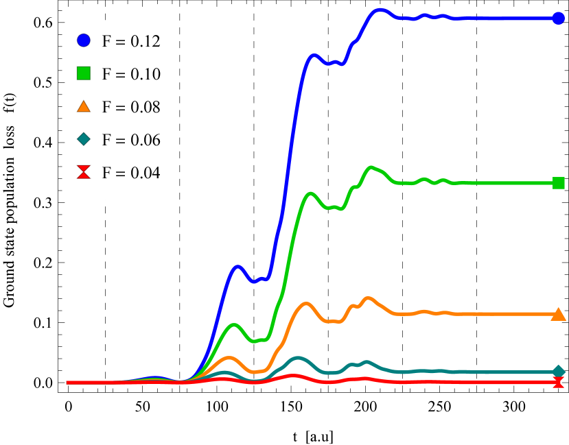
Figure 2: Time-dependence of the ground state population loss $f(t)$, defined in Eq. (16), for the indicated values of the parameter $F$, with $\mathrm{CEP}=0$. The $f(t)$ is linked to the probability of ionization. For pure tunnel ionization i.e. for $F<0.0624$, the ionization is very small. For higher values of $F$, the $f(t)$ rises suddenly around the peaks of the laser pulse.

We begin our analysis discussing the time-dependence of the ground state population loss (16) of the relative wave function, which is shown in Fig. 2 for several values of $F$. We can see sudden increases of the ground state population loss that are happening at the local extrema of the electric field, more and more clearly as $F$ increases. As we have already discussed in Section II, we make distinction between the tunneling ionization regime and the over-the-barrier ionization regime, regarding the dynamics dependent on $F$: starting from the former, we see from Fig. 2 that even for $F=0.06$, (just below the over-the-barrier threshold) the total ground state population loss is small ($0.02$) which implies small amount of ionization in the tunneling regime. At $F=0.10$ we have already a significant total ground state population loss ($0.33$) with prominent over-the-barrier ionization. At the highest $F$ shown ($F=0.12$), the electric field increasingly dominates the Coulomb force, and it almost doubles the total ground state population loss ($0.61$) and ionization.

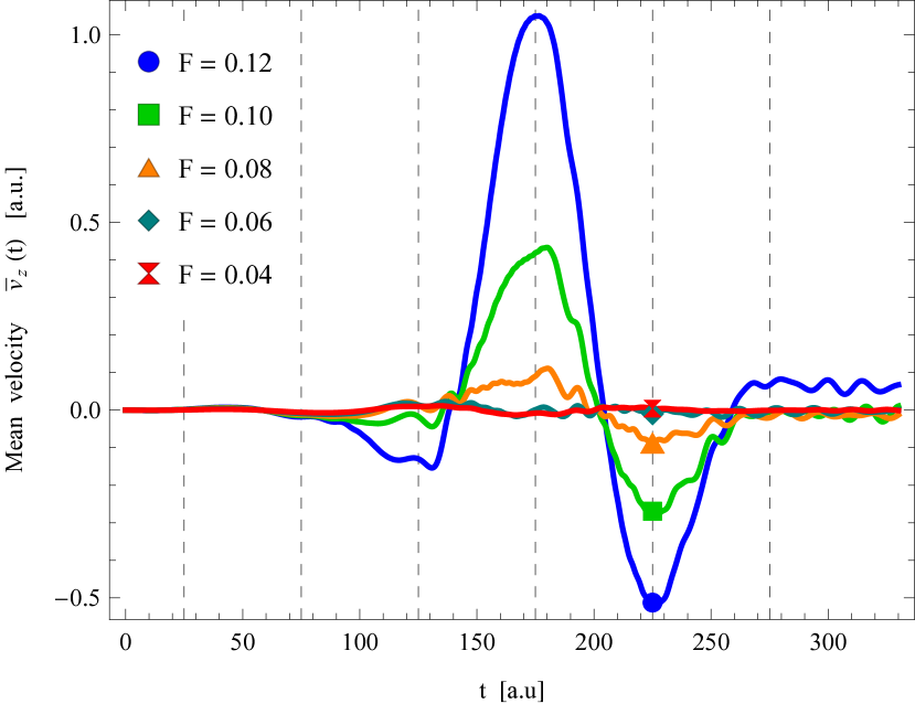
Figure 1: Time-dependence of the mean velocity of the relative wave function $\overline{v}_{z}(t)$, defined in Eq. (15), for the indicated values of the parameter $F$, with $\mathrm{CEP}=0$. For $F=0.12$, this velocity somewhat correlates with the quiver motion of the classical free electron moving under the influence of the same uniform dipole electric field (58). The vertical dashed lines denote the zero crossings of the electric field. (They have the same meaning on all of the figures.)

From Fig. 1, we can inspect how the results translate to an averaged classical motion, using the mean velocity component $\overline{v}_{z}(t)$ from the formula (15). In the tunneling range (with $F=0.06$ or below), $\overline{v}_{z}(t)$ only slightly changes with time and has oscillating component, which implies that the relative wave function is oscillating near the origin. For amplitudes sufficiently above the over-the-barrier ionization threshold $(F=0.1)$, the velocity somewhat correlates with the quiver motion of the classical free electron moving under the influence of the oscillating electric field (58). For example, $\overline{v}_{z}(t)$ has local extrema near the zero crossings of the electric field like within this classical picture. With increasing $F$, the correlation of $\overline{v}_{z}(t)$ and this “free” classical motion becomes more clear, signaling the increase of importance of the ionized waves. After the laser pulse ends, the ground state population loss stops as expected, and $\overline{v}_{z}(t)$ appears to oscillate near a constant mean value which is more remarkable with higher $F$. (This latter value can be nonzero, which contradicts the mentioned classical picture and the three step model.)

IV.4 Time-dependence of the quantum entropies

Now we start to analyze the time-dependent dynamics of the quantum entanglement of these ionization processes.

We begin the discussion of the various quantum entropies in the direction parallel to the laser polarization axis ($z$), then in the direction transverse to this polarization axis ($x$ or $y$) and in the last paragraphs in this subsection, we conclude with the discussion of the total electron-core entanglement approximated by our method. For this task, we set the electric field parameter to be $F=0.1$ which means an intermediate, over-the-barrier ionization range, and we choose the carrier envelope phase to be $\mathrm{CEP}=0$.

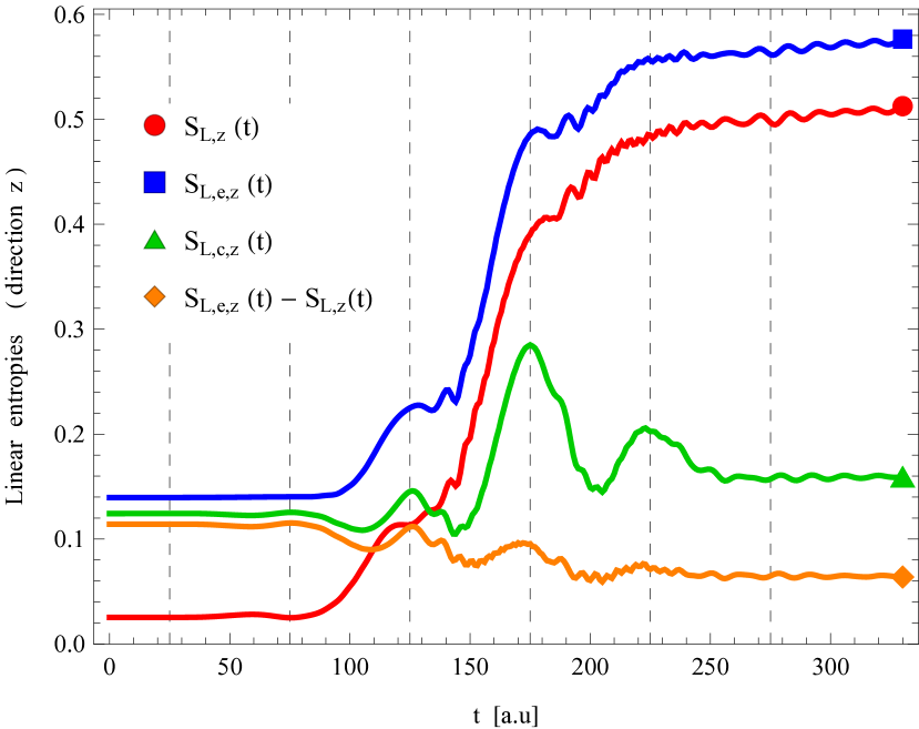
Figure 3: Comparison of the time-dependence of various linear entropies in direction $z$, based on our reduced density matrix formalism, using $F=0.1$, $\mathrm{CEP}=0$. Although the linear entropies of $S_{L,z}(t)$, $S_{L,c,z}(t)$, $S_{L,e,z}(t)$ compare fairly well to the respective Neumann entropies in Fig. 4, the negative linear conditional entropy $S_{L,e,z}(t)-S_{L,z}(t)$ gives a false prediction.

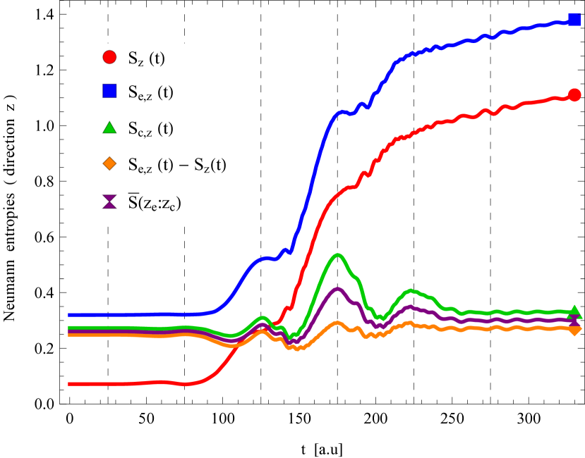
Figure 4: Comparison of the time-dependence of various Neumann entropies in direction $z$, based on our reduced density matrix formalism, using $F=0.1$, $\mathrm{CEP}=0$. The synchronous changes in $S_{c,z}(t)$, in $S_{e,z}(t)-S_{z}(t)$, and in $\overline{S}(z_{e}:z_{c},t)$ signal that they are related to a common source of correlation, which is primarily the quantum entanglement between $z_{e}$ and $z_{c}$, as evidenced by the high value of the negative conditional entropy $S_{e,z}(t)-S_{z}(t)$ .

First, we discuss the linear entropies of the reduced density matrices $\varrho_{z}$, $\varrho_{c,z}$ and $\varrho_{e,z}$. We use the notation $S_{L,z}(t)$, $S_{L,c,z}(t)$, $S_{L,e,z}(t)$ and we plot them in Fig. 3 to provide them as a comparison to the Neumann entropies $S_{z}(t)$, $S_{c,z}(t)$, $S_{e,z}(t)$, which are shown in Fig. 4, with the same parameters. Although these linear entropies compare fairly well to the respective Neumann entropies, the orange line in Fig. 3 shows that the quantity $S_{L,e,z}(t)-S_{L,z}(t)$ gives false prediction, therefore we use only the Neumann entropies, as we have already stated earlier.

The time-dependence of Neumann entropies corresponding to the direction $z$ are shown in Fig. 4. We see that $S_{z}(t)$ and $S_{e,z}(t)$ share the main features but $S_{c,z}(t)$ has a different behavior. First, let us say some words about the time dependence of the Neumann entropy $S_{z}(t)$ (plotted with red line). Overall, this spatial entropy of the “spatial entanglement” between $z$ and $\rho$ has major increase during the process due to the ionization: it starts from a rather small value of $0.07$ and and has a large permanent increase during the process (to the value $1.11$). This entropy also continues to grow slowly but steadily after the laser pulse ended, i.e. due to the mixing effect of the Coulomb potential only. It has sudden increases in time near the peaks of the laser pulse, however, with about 10 atomic time units of delays, with the biggest jump occurring near the central peak. If we compare this plot with the correspond curve of Fig. 1 we clearly see that the timings of these increases synchronize with the increases of $|\bar{v}_{z}(t)|$. Regarding the small starting value of $S_{z}(t)$, the initial state of $\exp(-\mu r)$ is almost separable in $z$ and $\rho$, in accordance with the low value of this entropy: particularly, the dominating eigenvalue of $\varrho_{z}$ at $t=0$ is $\lambda_{1}^{(z)}=0.9872$. This clearly shows that the Neumann entropies, in general, take into account the other much smaller eigenvalues in a more pronounced way.

In Fig. 4 we show the Neumann entropies $S_{e,z}(t)$ and $S_{c,z}(t)$, and the negative conditional entropy $S_{e,z}(t)-S_{z}(t)$, with blue, green and orange lines, respectively, in order to attempt to answer the question, how the core-electron correlation works in the directional $z$ subsystem. We stated in Section III, that the coordinate transformation (28) creates a special type of correlation. Therefore, we should be able to acquire (at least partially) the correlation information contained in $S_{c,z}(t)$ from the Neumann entropy $S_{e,z}(t)$. As it is clearly shown by Fig. 4, the majority of the time-dependent features of $S_{e,z}(t)$ seem to be inherited from the Neumann entropy of the reduced density matrix $\varrho_{z}(t)$ (for example, the sudden increases related to the ionization), they are only shifted to higher values. However, if we carefully inspect the curve of $S_{e,z}(t)-S_{z}(t)$ in Fig. 4 (in orange) we can easily observe that its main features (like its correlation with the laser pulse) are very similar to those of $S_{c,z}(t)$. Because these quantities are close to each other, it means that in this subsystem the major correlation is quantum entanglement, as we stated earlier. Therefore, $\overline{S}(z_{c}:z_{e},t)$, defined in (81), can be used as an approximate entanglement measure. We also make the observation that $S_{z}(t)$ is always upper bounded by $S_{e,z}(t)$, and the respective $z$ coordinate of the lighter electron contains more entropy than that of the heavier ion-core, as expected.

Next, we discuss the time dependence of the resulting mutual entropy $\overline{S}(z_{c}:z_{e},t)$, which is plotted in Fig. 4 as a purple curve. This quantity inherits its features from $S_{c,z}(t)$ and $S_{e,z}(t)-S_{z}(t)$ by construction: it starts from an intermediate value ($0.23$), rises and falls several times during the process, contrary to $S_{z}(t)$. It stays almost constant after the laser pulse, around a value ($0.25$) that is only slightly higher than the initial value. The time-dependence of $\overline{S}(z_{c}:z_{e},t)$ correlates better with the shape of the laser pulse, and also has much smaller peak value in the time window, than the aforementioned spatial entropy. Interestingly, the rapid changes in ionization probability during the process are not reflected by this particle-particle entanglement of the $z$ directional subspace. The changes of this mutual entropy are more correlated with the average velocity $\overline{v}_{z}(t)$, which we expand more in the next subsection.

The curves of Fig. 4 clearly show that the classical correlations also change under the effect of the laser pulse: the gap between $S_{c,z}(t)$ and $S_{e,z}(t)-S_{z}(t)$ is dynamically increasing and decreasing, synchronously with the electric field. Even though the respective mutual entropy includes these classical effects, the also synchronous changes in $S_{c,z}(t)$ and in $S_{e,z}(t)-S_{z}(t)$ signal that the quantum entanglement behaves the same way, and the high value of the negative conditional entropy causes it to be the major correlation.

Here we ought to note that the actual related values of $S_{c,z}(t)$, $\overline{S}(z_{c}:z_{e},t)$, $S_{e,z}(t)-S_{z}(t)$ are also influenced by $\Psi_{0}$, that is by the adjustable parameter $\sigma^{2}$. According to our simulations, the change of $\sigma^{2}$ does not affect the aforementioned observations of the time-dependent characteristics of these entropies. The major difference between different values of $\sigma^{2}$ is that it results in a shift of the values $\overline{S}(z_{c}:z_{e},t)$ and it affects the already slow dispersion rate of $\Psi_{0}$.

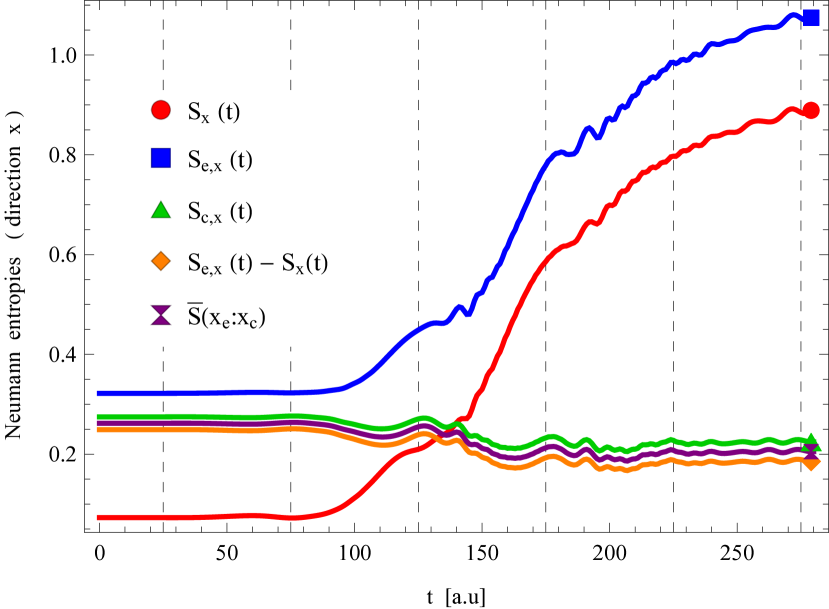
Figure 5: The time evolution of the various Neumann entropies based on the reduced density matrices in direction $x$, using the parameters $F=0.1$, $\mathrm{CEP}=0$. We can see that the $\overline{S}(x_{e}:x_{c},t)$ shares time-dependent features with $\overline{S}(z_{e}:z_{c},t)$, for example, its maxima are near the zero crossings of the laser pulse. The major correlation between $x_{e}$ and $x_{c}$ is quantum entanglement.

The time-dependence of the same of quantum entropies which characterize the reduced dynamics along the $x$ axis (same along $y$) can be seen in Fig. 5. However, we limited the range of the time axis (to $280$ atomic time units) in this case, since one of this entropy calculations is done about $O(N^{4})$ steps instead of $O(N^{3})$, and it also involves that much interpolation in order to do integration in Cartesian coordinates.

From Fig. 5, we can see a familiar shape related to the spatial entropy in the form of $S_{x}(t)$, because the values of the Neumann entropy $S_{x}(t)$ mirrors that of $S_{z}(t)$, but they are not the same. However, they are actually identical at $t=0$ due to the spherical symmetry of $1s$ Coulomb state, i.e. (a single index) tripartite Schmidt decomposition Pati (2000) of the initial relative wave function exists. Then the laser pulse causes this wave function to slowly depart from this tripartite Schmidt state as $S_{x}(t)$ and $S_{z}(t)$ differ more. However, both $S_{x}(t)$ and $S_{z}(t)$ depict the time dependence of spatial entropy adequately.

Now we turn our attention to the particle-particle correlation of the $x_{e}$ and $x_{c}$ coordinates. First, this correlation is quantum entanglement because $S_{c,x}(t)$ and its negative conditional entropy i.e. $S_{e,x}(t)-S_{x}(t)$ stay really close to each other which is only possible if $x_{e}$ and $x_{c}$ are entangled, therefore $\overline{S}(x_{e}:x_{c},t)$ is a good entanglement measure. Now, we can also see that the $\overline{S}(x_{e}:x_{c},t)$ shares some time-dependent features with $\overline{S}(z_{e}:z_{c},t)$, for example, its maxima are near the zero crossings of the laser pulse. Note, however, that the changes in $\overline{S}(x_{e}:x_{c},t)$ are considerably smaller than those in $\overline{S}(z_{e}:z_{c},t)$. It is somewhat surprising that there is an overall entanglement decrease in direction $x$, which we discuss in the next subsection in more detail. This decrease could be an evidence of the purification between the two subsystems $x_{e}$ and $x_{c}$, as these coordinates become more uncorrelated during the physical process.

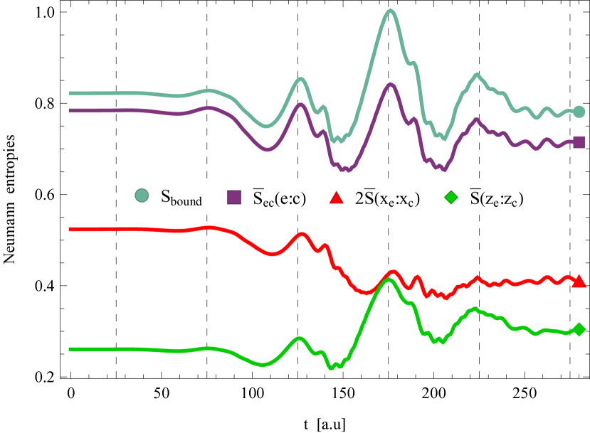
Figure 6: The time evolution of our electron-core entanglement entropy $\overline{S}_{ec}(e:c,t)$ and the upper bound of the analytic entanglement entropy $S_{\mathrm{bound}}(t)$, along with time evolution of the directional entropies $2\overline{S}(x_{e}:x_{c},t)$ and $\overline{S}(z_{e}:z_{c},t)$ with parameters $F=0.1$, $\mathrm{CEP}=0$. The time dependence of $S_{\mathrm{bound}}(t)$ and $\overline{S}_{ec}(e:c,t)$ follow each other with substantial, and slightly increasing gap which indicates the actual importance of these curves. The total entanglement entropy reaches a net decrease by the end of the laser pulse. Important features of $\overline{S}_{ec}(e:c,t)$ are shared with $\overline{S}(z_{e}:z_{c},t)$ (like the correlation with the external electric field, and the definite positions of the maxima near the zero crossings of the laser field) which suggests that the relevant physics happens along the polarization axis.

Finally, in Fig. 6, we plot the result of our approximate formula $\overline{S}_{ec}(e:c,t)$ of the physical core-electron entanglement using (53) with its analytic upper bound $S_{\mathrm{bound}}(t)$ via (44). There, we also plot the function $\overline{S}(x_{e}:x_{c},t)+\overline{S}(y_{e}:y_{c},t)=2\overline{S}(x_{e}:x_{c},t)$ and $\overline{S}(z_{e}:z_{c},t)$ for the $z$ subsystem. We see that our approximate quantification formula $\overline{S}_{ec}(e:c,t)$ is clearly below $S_{\mathrm{bound}}(t)$, with substantial, and slightly increasing gap. Also the time dependence of these follow each other, which indicates the actual importance of $\overline{S}_{ec}(e:c,t)$. It seems to be surprising that the total entanglement entropy shows a net decrease by the end of the laser pulse, which we will revisit in the next subsection. This is especially interesting when we take into account that other important features of the entropy $\overline{S}_{ec}(e:c,t)$ mimic those of the mutual entropy $\overline{S}(z_{e}:z_{c},t)$. In this sense we could say that the part of the relevant physics happens along the polarization axis (like the correlation with the external electric field, and the definite positions of the maxima near the zero crossings of the laser field) but the perpendicular degrees of freedom change the overall dynamics of the entanglement from increasing to decreasing.

We will further explore the dynamics of all types of entanglement presented so far in the following subsections, while also giving more insight into the physics, by changing the external field that governs the process.

IV.5 Parameter dependence of the quantum entropies: electric field strength

In this section we discuss the dependence of the important entanglement entropies of Section III on the parameter $F$ i.e. on the strength of the external electric field.

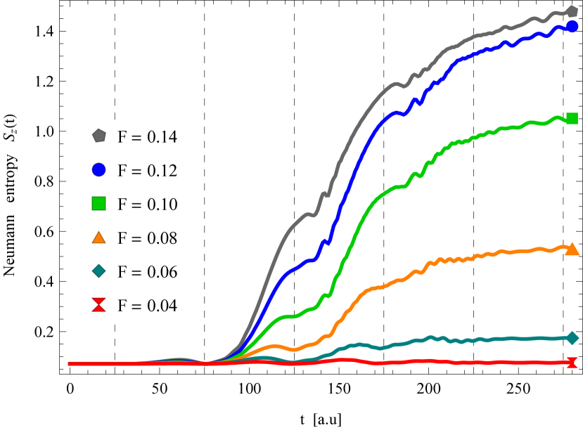
Figure 7: The time evolution of the Neumann entropy $S_{z}(t)$ for the indicated values of the parameter $F$, with $\mathrm{CEP}=0$. Below the value $F=0.04$, we have only a negligible increase in $S_{z}(t)$, i.e. the relative wave function stays nearly separable in $z$, $\rho$ during the process. This separability quickly breaks down with increasing $F$. The fast rises of $S_{z}(t)$ are related to the sudden changes of ionization probability, see Fig. 2.

In Fig. 7 we plot the spatial entropy $S_{z}(t)$ for the relevant values of $F$ . Comparing these curves with the ground state population loss of Fig. 2 it is easy to correlate the time evolution of $S_{z}(t)$ to the probability of ionization.

Note that below the value $F=0.04$, we have only a marginal increase in $S_{z}(t)$, i.e. the relative wave function stays nearly separable in $z$, $\rho$ during the process. This separability quickly breaks down with increasing $F$, which is an important information regarding the applicability of the time-dependent multiconfigurational Hatree approaches (Beck et al., 2000) for the simulations of strong field processes. It is also interesting that we have not found any specific mark of the tunneling or the over-the-barrier ionization regimes. Between $F=0.12$ and $F=0.14$, the entropy increase already slows down as a function of $F$, and one can extrapolate that the spatial nonseparability has a saturation point near $F=0.14$. We verified the existence of this maximum value with additional computations. Therefore, there is a limiting maximal value for $S_{z}(t)$ in the given time window, which already corresponds also to nearly complete ionization. The $S_{z}(t)$ is not only the measure of “spatial entanglement”, but it is also the total entropy of the $z$ subsystem, which has consequences regarding the interpretation of the directional mutual entropies.

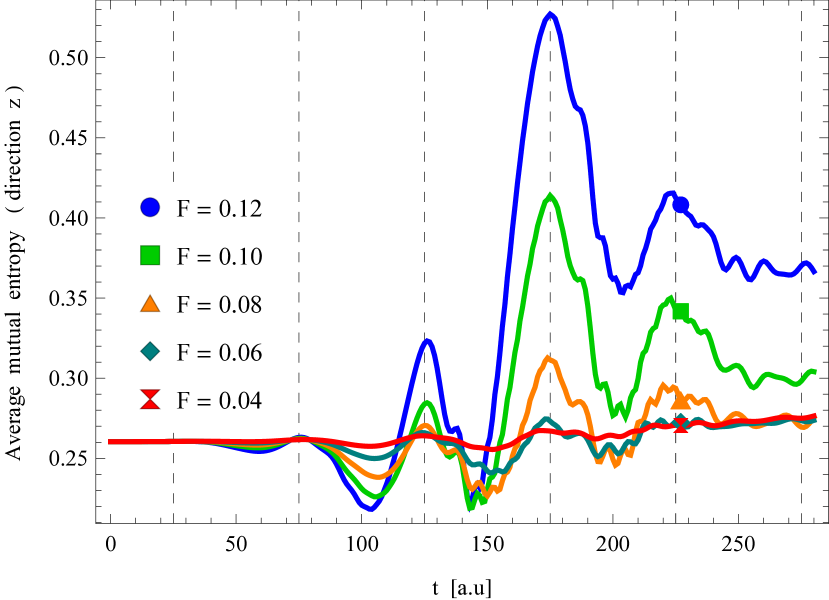
Figure 8: The time evolution of the mutual entropy $\overline{S}(z_{e}:z_{c},t)$ for the indicated values of the parameter $F$, with $\mathrm{CEP}=0$. By comparing to Fig. 1, we can easily recognize that the mean relative velocities $\overline{v}_{z}(t)$ are tied to the quantum entanglement in direction $z$. These curves are very similar to the exact quantum entanglement entropy curves in Fig. 1. of our former 1D model simulation Czirják et al. [2013]. The local maxima increase with increasing $F$, the largest change occurring at the main maximum ($t=175$). Positions of the local maxima almost coincide with the zero crossings of the laser’s electric field.

In Fig. 8 we plot the average mutual entropy in the directional $z$ subsystem, $\overline{S}(z_{e}:z_{c},t)$, for the relevant range of $F$. It is easy to see that the correlation of this entropy with the shape of the laser pulse becomes more clear as we increase $F$. The values of the first minima decrease as $F$ increases, but this is reversed for the other local minima. Regarding the local maxima, they all increase with increasing $F$, the largest change occurring at the main maximum ($t=175$). Positions of the local maxima are independent of $F$. We can observe a tunneling regime feature: the value of this entropy returns to the baseline at the end of the laser pulse. As the over-the-barrier ionization takes over ( above $F=0.08$) the final value of the entanglement between $z_{e}$ and $z_{c}$ rises with increasing $F$ .

Comparing Fig. 8 and Fig. 1, it is easy to recognize that the mean relative velocities $\overline{v}_{z}(t)$ (or alternatively, momenta) play a particularly important role regarding quantum entanglement in this direction. During one half cycle of the laser pulse, as the core and the electron are moving apart, the entanglement of their respective coordinates $z_{e}$ and $z_{c}$ increases proportionally to the magnitudes of their relative velocities. The value of their entanglement decreases when deceleration occurs, and reaches its minimum value when the particles’ relative motion stops. The final value of entanglement is also related to this velocity.

The results presented in Fig. 8 are even more interesting if we compare them to the exact quantum entanglement entropy curves in Fig. 1. of our former 1D model simulation (Czirják et al., 2013). Despite that the average mutual entropy $\overline{S}(z_{e}:z_{c},t)$ includes an increasing “background” (since the composite system is always in a mixed state in the 3D model), the main features of the temporal dependence in Fig. 8 and in Fig. 1. of (Czirják et al., 2013) exhibit a very good qualitative agreement: the position of the local maxima coincide with the zeros of the laser pulse, the main maximum of the entropy is roughly the double of its initial value, and the asymptotic value at the end of the simulation time scales roughly the same way to the corresponding maximum values. This agreement strongly supports our opinion that the average mutual entropy $\overline{S}(z_{e}:z_{c},t)$ is a useful measure of quantum entanglement for the degrees of freedom along the direction of the laser polarization in the 3D case. The agreement also justifies the use of the delta-potential in the 1D simulation, because the resulting exact core-electron quantum entanglement quantitatively correctly describes the corresponding entanglement dynamics of the 3D case.

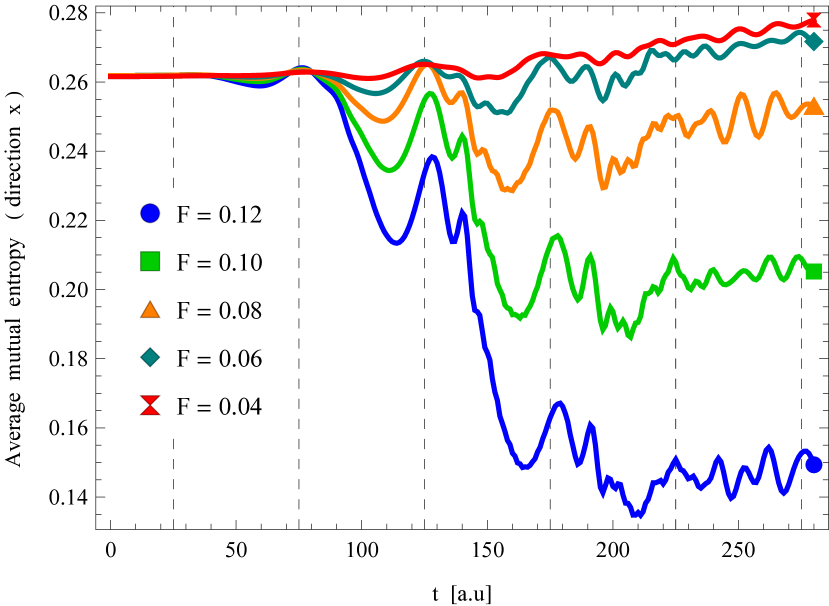
Figure 9: The time evolution of the mutual entropy $\overline{S}(x_{e}:x_{c},t)$ for the indicated values of the parameter $F$, with $\mathrm{CEP}=0$. This figure shows more clearly the striking feature that was already present in Fig. 5: the average mutual entropy in the direction $x$ decreases surprisingly strongly with increasing $F$ in the over-the-barrier ionization regime.

Regarding the transverse direction $x$, first we note that the time dependence of $S_{x}(t)$ is very similar to that of $S_{z}(t)$ and it scales with $F$ also in an analogous way, therefore we do not plot $S_{x}(t)$. We plot $\overline{S}(x_{e}:x_{c},t)$ in Fig. 9 in analogy to Fig. 8. This figure shows more clearly the striking feature that was already present in Fig. 5: the average mutual entropy in the transverse direction decreases surprisingly strongly with increasing $F$ in the over-the-barrier ionization regime. This unexpected behavior is of purely quantum mechanical nature, contrary to direction $z$: since $\overline{v}_{x}(t)=0$, there is no “classical” explanation based on the Ehrenfest kinematics. However, the positions of the local maxima $\overline{S}(x_{e}:x_{c},t)$ are still tied to the zero crossings of the laser field. There is an importance of the tunneling regime ($F=0.0624$ and below), where the average mutual entropies $\overline{S}(x_{e}:x_{c},t)$ and $\overline{S}(z_{e}:z_{c},t)$ have almost the same overall behavior and show an entropy increase.

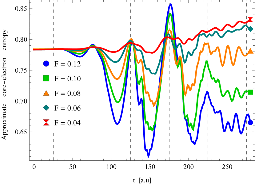
Figure 10: The time evolution of the approximate core-electron entropy $\overline{S}_{ec}(e:c,t)$ for the indicated values of the parameter $F$, with $\mathrm{CEP}=0$. Due to its construction, it inherits its features from $\overline{S}(z_{e}:z_{c},t)$ and $\overline{S}(x_{e}:x_{c},t)$. Surprisingly, the entropy decrease of the transverse directions dominate the entropy increase in direction $z$, therefore this approximate core-electron entanglement decreases with increasing $F$ in the over-the-barrier ionization regime.

Finally, in Fig. 10, we plot the approximate core-electron entanglement $\overline{S}_{ec}(e:c,t)$, defined in Eq. (53). Due to its construction, it inherits its features from $\overline{S}(z_{e}:z_{c},t)$ and $\overline{S}(x_{e}:x_{c},t)$ in the following way: if the value of $F$ ensures pure tunnel ionization, then $\overline{S}_{ec}(e:c,t)$ gains a net increase by the end of the laser pulse, otherwise the core-electron entanglement decreases with increasing $F$, which is a rather surprising result. Other important features of $\overline{S}(z_{e}:z_{c},t)$ are preserved also for $\overline{S}_{ec}(e:c,t)$: the presence of the local maxima at the zero crossings of the laser field, the general nature of the correlations, and its link to the mean velocity.

IV.6 Parameter dependence of the quantum entropies: carrier envelope phase

In this section we investigate the effects of the carrier envelope phase ($\mathrm{CEP)}$ on the process.

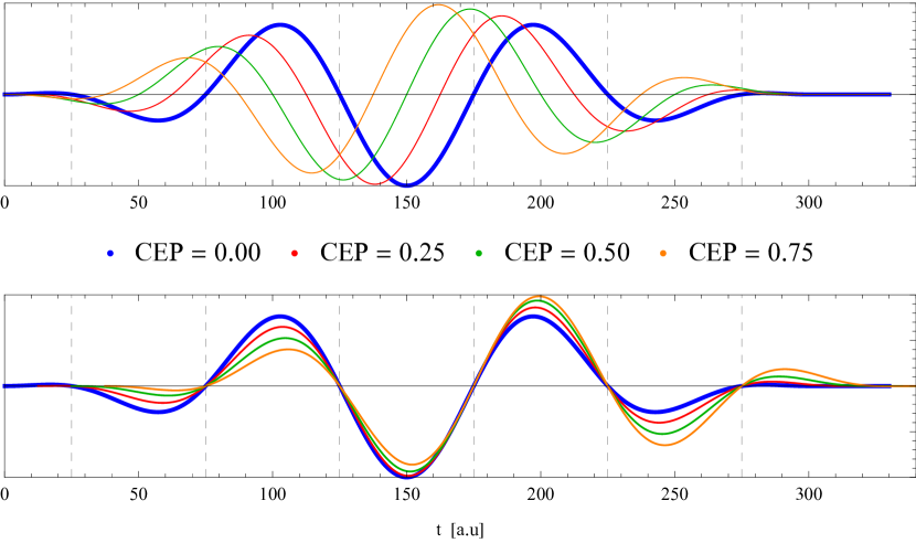
Figure 11: Plots of the laser pulses’ electric fields $E_{z}(t)$ versus time with four selected values of the parameter $\mathrm{CEP}$, where the thick blue curves indicate the case of $\mathrm{CEP=}0$. The vertical axes range from $-F$ to $F$ and represent the strength of the electric field. Plots in the upper panel are according to the formula (58) then we applied a $\mathrm{CEP}$ dependent shift in time to make the zero crossings coincide (lower panel). We plot the time-dependence of some selected quantities in Figures 12 to 16 with this shift applied.

In the upper panel of Fig. 11 we plot the electric field of the laser pulse for our selected $\mathrm{CEP}$ values, with the strength of the electric field parameter set to $F=0.1$. For the sake of better comparability, we apply the following $\mathrm{CEP}$ dependent transformation in time: we shift backwards the time domains in the case of nonzero $\mathrm{CEP}$ values such that the zero crossings of the various laser pulses coincide, as shown in the lower panel of Fig. 11. We plot the time dependence of some selected quantities in the following figures with this shift applied.

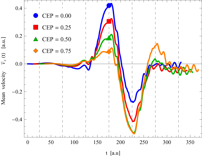
Figure 12: Plots of the mean velocity $\overline{v}_{z}(t)$ of the relative wave function versus time for the indicated $\mathrm{CEP}$ parameters, with $F=0.1$.

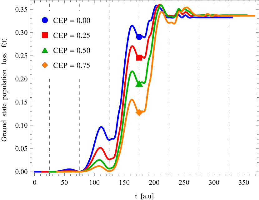
Figure 13: Plots of the ground state population loss of the relative wave function versus time for the indicated $\mathrm{CEP}$ parameters, with $F=0.1$.

We plot the $\mathrm{CEP}$ dependence of the ground state population loss in Fig. 13 and the mean velocity $\overline{v}_{z}(t)$ in Fig. 12 using the above mentioned transformation. For each $\mathrm{CEP}$ value, the dynamical properties of the system stay synchronized to the local minima, maxima and zero crossings of the laser pulses. The values of the ground state population loss at the end of the laser pulse are nearly unaffected by the parameter $\mathrm{CEP}$. The corresponding values of $\overline{v}_{z}(t)$ are only slightly affected by the $\mathrm{CEP}$ change.

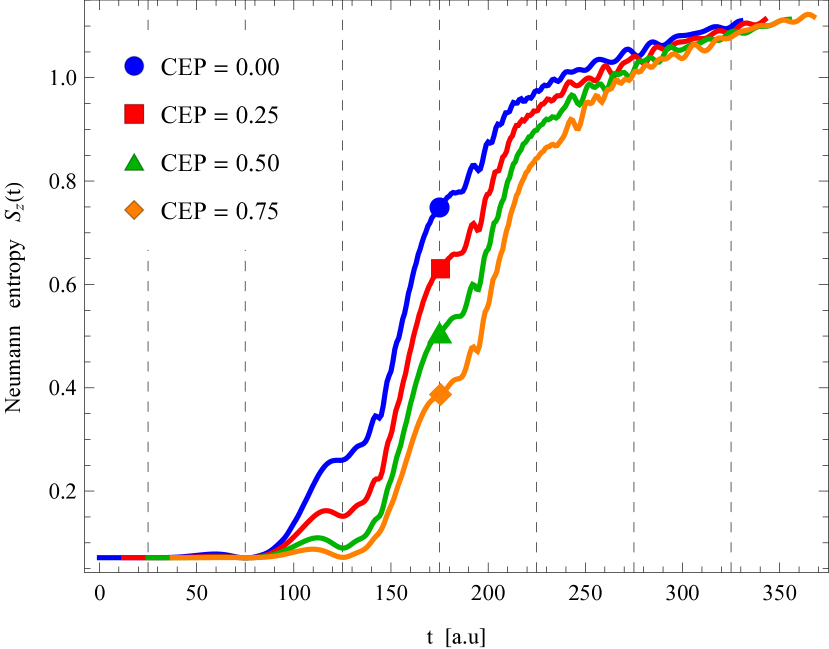
Figure 14: Plots of the Neumann entropy $S_{z}(t)$ versus time for the indicated $\mathrm{CEP}$ parameters, with $F=0.1$.

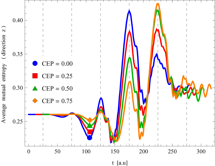
Figure 15: The plot of the mutual entropy $\overline{S}(z_{e}:z_{c},t)$ for the indicated $\mathrm{CEP}$ parameters, with $F=0.1$. Note that the peak at $t=175$ shrinks as the $\mathrm{CEP}$ increases while the peak at $t=225$ increases.

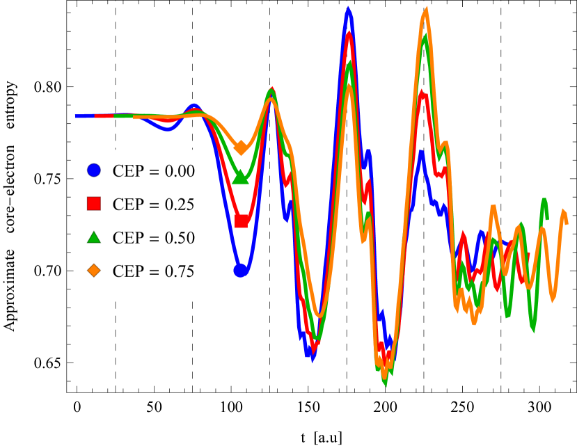
Figure 16: The plot of the electron-core entropy $\overline{S}_{ec}(e:c,t)$ for the indicated $\mathrm{CEP}$ parameters, with $F=0.1$.

The entanglement properties of the system inherit the above $\mathrm{CEP}$ related features. To show this, we plot the $\mathrm{CEP}$ dependence of the entropy of the “spatial entanglement” in Fig. 14, the entropy of nonseparability in direction $z$ in Fig. 15, and our approximated core-electron entanglement entropy in Fig. 16 including already the $\mathrm{CEP}$ dependence in direction $x$. In the latter two Figures, we can see that the local maxima still coincide with the zeros of the electric fields, independently of the $\mathrm{CEP}$ values, and the $\mathrm{CEP}$ has barely any effect on the final values. However, the actual values of the ionization, the velocities and all the entropies change considerably with respect to each other between subsequent half cycles, depending on the value of the $\mathrm{CEP}$ parameter. For example, in Fig. 14 the peak at $t=175$ shrinks as $\mathrm{CEP}$ increases and the peak value at $t=225$ grows synchronously. We have found it interesting that the latter entropy acquires its largest value near $\mathrm{CEP}=0.75$ and not $\mathrm{CEP}=0.0$, where we have the largest value of $E_{z}(t)$. Thus, although the parameter ${\rm CEP}$ changes the sub-cycle dynamics of both these entropies considerably, its value does not affect our main observations about the overall time-dependent entropy dynamics.

V Summary

In this paper, we applied the theory of quantum entanglement and the concepts of quantum information theory to describe the time-dependent correlation properties of an electron and its parent ion-core under the influence of an external laser pulse which is strong enough to liberate the electron by tunnel or by over-the-barrier ionization. The computation of the standard entanglement measure i.e. the Neumann entropy of either the electron or the core density matrix for this problem is numerically prohibitive in its full dimensionality, therefore we choose to partition the interacting system along the spatial directions parallel and perpendicular to the laser polarization axis, denoted by $z$ and $x$, respectively. These direction-wise reduced dynamics still retain all pair correlations in $x$ and $z$. To analyze the corresponding pair correlations between the electron and the ion-core coordinates, we used several kinds of Neumann entropies that can be calculated from the one-dimensional density matrices of the system. Based on the concepts of quantum conditional entropy and quantum mutual entropy, we introduced average mutual entropies between the electron’s and the ion-core’s spatial position along the $x$ and $z$ directions as suitable and useful correlation measures. We constructed an approximate formula, Eq. (53), to quantify the total particle-particle entanglement between the electron and the ion-core, based on the direction-wise mutual entropies.

We analyzed the nature of the correlations in each direction and we found that they are based on the same fundamental features of this system. For example in direction $z$, the ion-core entropy $S_{c,z}(t)$ behaves like a correlation entropy, because the ion-core density matrix is close to that of the center of mass which has zero entropy. The spatial entropy $S_{z}(t)$ is concentrated in the direction-wise electron entropy $S_{e,z}(t)$, which also incorporates a correlation part. The resulting $S_{e,z}(t)-S_{z}(t)$, which is the negative conditional entropy of the ion-core, becomes positive and has many features in common with $S_{c,z}(t)$. In most of the simulations, these two stay really close to each other, which means that the state as the function of the $z_{e}$ and $z_{c}$ coordinates shows dominantly quantum entanglement. The same is true with respect to the $x_{e}$ and $x_{c}$ coordinates. This behavior is very different from pure state entanglement, because these directional subsystems are in mixed states.

We analyzed the correlation entropy relations in each direction and we found that the zero crossings of the electric field almost coincide with their local maxima. These results in direction $z$ are also in a good agreement with our earlier one dimensional simulations. The correlations along the $x$ and $z$ directions are very similar to each other if the process stays in the tunnel ionization regime. In the over-the-barrier ionization regime, we found entropy increase along $z$ but a surprising entropy decrease in the transverse directions which makes also the total core-electron entanglement entropy to decrease, contrary to what we expected.

We investigated the dependence of these proposed measures of entanglement dynamics on the strength and the carrier-envelope phase of the driving laser pulse. We found many features of quantum entropies that do not depend on these parameters, like the electron-core entanglement has local maxima always near the zero crossings of the laser pulse. We found that while the intensity of the field governs the dynamics as a whole, the carrier envelope phase changes the sub-cycle dynamics of the strong field ionization.

Based on our simulations, we also calculated some relevant quantities that contribute to the physical picture of strong field ionization. We found that the ground state of the simulated relative wave function is almost separable, and it remains so if the field is weak. The loss of the ground state population is a good measure of ionization, and that the net effect of the ionized waves results in a mean velocity $v_{z}(t)$ which is more and more similar to the corresponding motion of a classical electron as the laser intensity increases, apart from the nonzero final velocity.

We think that our results will be useful regarding the interpretation of quantum measurements, especially in connection with strong-field processes, using e.g. COLTRIMS or other reaction microscopes Dörner et al. (2000); Ullrich et al. (2003). An obvious but not trivial extension of our present work could be the calculation of electron entanglement in double ionization Becker et al. (2012). We also hope to inspire further developments in quantum information theory.

Appendix A Quantification of bipartite quantum entanglement

A.1 Schmidt decomposition and entanglement

In this appendix we recall the standard theory of quantum entanglement for bipartite systems emphasizing the features specific to states described by square integrable coordinate wave-functions of infinite dimensional Hilbert spaces. In our problem the two parts $e$ and $c$, are two distinguishable particles, the electron and its parent ion-core. The composite system $ec$ is assumed to be a closed quantum system in a pure state represented by the wave function $\Psi_{ec}(\mathbf{r}_{e},\mathbf{r}_{c},t)$. The two subsystems are entangled if $\Psi_{ec}$ is not separable with respect to the coordinates of these subsystems:

$$\Psi_{ec}(\mathbf{r}_{e},\mathbf{r}_{c},t)\neq\Psi_{e}(\mathbf{r}_{e},t)\Psi_{c}(\mathbf{r}_{c},t).$$ (59)

It is well-known that then the result of the measurement of subsystem $e$ affects the outcome of measurements on subsystem $c$ and vice-versa. That is, performing measurement on either particle changes the other particle’s quantum state in a nonlocal manner.

To quantify the entanglement, we need the relevant concept of density matrices. The composite system is described by the two-particle pure state density matrix:

$$\varrho_{ec}(\mathbf{r}_{e}^{\prime},\mathbf{r}_{e},\mathbf{r}_{c}^{\prime},\mathbf{r}_{c},t)=\Psi_{ec}^{\ast}(\mathbf{r}_{e}^{\prime},\mathbf{r}_{c}^{\prime},t)\Psi_{ec}(\mathbf{r}_{e},\mathbf{r}_{c},t).$$ (60)

and the single particle density matrices are obtained by tracing over the other particle’s degrees of freedom. The reduced single particle core density matrix is

$$\varrho_{c}(\mathbf{r}_{c}^{\prime},\mathbf{r}_{c},t)=\mathrm{Tr}_{e}\left[\hat{\varrho}_{ec}\right]=\int\varrho_{ec}(\mathbf{r}_{e},\mathbf{r}_{e},\mathbf{r}_{c}^{\prime},\mathbf{r}_{c},t){\rm d}\mathbf{r}_{e}^{3}$$ (61)

and the reduced single particle electron density matrix is

$$\varrho_{e}(\mathbf{r}_{e}^{\prime},\mathbf{r}_{e},t)=\mathrm{Tr}_{c}\left[\hat{\varrho}_{ec}\right]=\int\varrho_{ec}(\mathbf{r}_{e}^{\prime},\mathbf{r}_{e},\mathbf{r}_{c},\mathbf{r}_{c},t){\rm d}\mathbf{r}_{c}^{3}.$$ (62)

These quantities contain every quantum information about the respective single particle properties, and they are directly related to the entanglement information we need. To show this, we refer to the Schmidt theorem (Eberly, 2006; Luo and Zhang, 2003), which states that there exists a unique decomposition of the entangled wavefunction $\Psi_{ec}$ of the bipartite system $ec$ into a sum of the following form:

$$\Psi_{ec}(\mathbf{r}_{e},\mathbf{r}_{c},t)=\sum\limits_{k}\sqrt{\lambda_{k}(t)}\phi_{k}(\mathbf{r}_{c},t)\psi_{k}(\mathbf{r}_{e},t).$$ (63)

where $\phi_{k}(\mathbf{r}_{c},t)$ and $\psi_{k}(\mathbf{r}_{e},t)$ are orthonormal basis functions in the respective spaces. They are acquired after the diagonalization of the single particle reduced density matrices (61) and (62) as

$$\varrho_{e}(\mathbf{r}_{e}^{\prime},\mathbf{r}_{e},t)=\sum\limits_{k}\lambda_{k}(t)\psi_{k}^{\ast}(\mathbf{r}_{e}^{\prime},t)\psi_{k}(\mathbf{r}_{e},t),$$ (64)

$$\varrho_{c}(\mathbf{r}_{c}^{\prime},\mathbf{r}_{c},t)=\sum\limits_{k}\lambda_{k}(t)\phi_{k}^{\ast}(\mathbf{r}_{c}^{\prime},t)\phi_{k}(\mathbf{r}_{c},t),$$ (65)

i.e the formula (63) contains the eigenvectors $\phi_{k}$, $\psi_{k}$ as the Schmidt basis functions, and the countably many common eigenvalues $\lambda_{k}(t)$ of $\varrho_{e}$ and $\varrho_{c}$ density matrices respectively. We note that in this continuous variable case the diagonalization of (61) or (62) actually involves the solution of a homogenous Fredholm integral equation of the second kind. In addition – contrary to discrete variable systems – these density matrices are usually highly singular, due to the trace condition Tr$\varrho_{e}$=Tr$\varrho_{c}=1$ they contain infinitely many zero or close to zero eigenvalues. Therefore, it is necessary to introduce an ordering of the eigenvalues $\lambda_{1}\geq\lambda_{2}\geq\lambda_{3}\geq\ldots$ and then to use only a finite number of them which are greater than an adequately small threshold number $\epsilon$.

The eigenvalues $\lambda_{k}(t)$  allow one to quantify the entanglement of the particles (subsystems) $e$ and $c$ by introducing quantum entropies (Eltschka and Siewert, 2014; Lin and Ho, 2014). Most frequently we use here the von Neumann entropy

$$S_{N}(t)=-\mbox{Tr}\left[\hat{\varrho}_{c}(t)\ln\hat{\varrho}_{c}(t)\right]=-\sum\limits_{k}\lambda_{k}(t)\ln\lambda_{k}(t),$$ (66)

and in certain cases the linear entropy

$$S_{L}(t)=1-\mbox{Tr}\left[\hat{\varrho}_{c}^{2}(t)\right]=1-\sum\limits_{k}\lambda_{k}^{2}(t).$$ (67)

The von Neumann entropy obeys some natural requirements, and it also has a quantum information theoretic appeal (Schumacher, 1995) while the linear entropy (67) is easier to calculate, since diagonalization is not necessary. However, both of these entropies generally tend to behave the same way in this simple bipartite configuration: if a subsystem is in a pure state they assume the value $0$, and they increase as the “mixedness” of the subsystem’s state increases . It is important that this quantification does not straightforwardly generalize to the case where the composite system is divided into more than two subsystems Carteret et al. (2000).

For independent systems the total density operator is the tensorial product of those of the subsystems and then the Neumann entropy of the composite system is exactly the sum of the Neumann entropies of the subsystems. In our case, however, when by the very nature of the problem $e$ and $c$ are not independent, only strong subadditivity holds (Wehrl, 1978), which gives an upper bound of the composite system’s entropy as

$$S_{N}(\varrho_{ec})\leq S_{N}(\varrho_{e})+S_{N}(\varrho_{c}),$$ (68)

A useful lower bound is given by Araki-Lieb inequality as

$$\left|S_{N}(\varrho_{e})-S_{N}(\varrho_{c})\right|\leq S_{N}(\varrho_{ec}).$$ (69)

A.2 Correlation types and quantum information

In general, $\varrho_{ec}$ involves both classical and quantum correlations. Then it is crucial to recognize the features of these, and to do that, we recall their meaning first. If a bipartite system contains only classical correlations between the two subsystems, then it has a density matrix of the following form:

$$\varrho_{ec}^{\mathrm{(cl)}}=\sum_{k}w_{k}\cdot\varrho_{e}^{(k)}\otimes\varrho_{c}^{(k)},$$ (70)

where $w_{k}$ satisfy $\sum_{k}w_{k}=1$ and $w_{k}\geq 0$. We are dealing with some form of quantum entanglement only if the density matrix of the system does not satisfy (70). We denote the corresponding class of nonclassical density matrices generally as $\varrho_{ec}^{({\rm quant})}$. A special case of this is the entangled pure state density matrix $\varrho_{ec}^{{\rm(pure})}$ defined in (60) which will serve as an important analytic example for quantum entanglement.

In the following, we recall relevant entropic quantities of quantum information theory that suit the task of determination and quantification of entanglement. We will denote the composite system by $EC$, and its subsystems by $E$ and $C$. We also simplify the notation of the entropies as $S(EC)=S_{N}(\varrho_{ec})$, $S(E)=S_{N}(\varrho_{e})$, $S(C)=S_{N}(\varrho_{c})$.

A.3 Quantum conditional entropy

The quantum conditional entropy corresponding to a subsystem can be introduced based on the conditional density or amplitude operator (Cerf and Adami, 1997, 1999), but we consider the following formula for the definition

$$S(E|C)=S(EC)-S(C)$$ (71)

for the quantum conditional entropy of subsystem $E$, and $S(C|E)$ is the quantum conditional entropy of subsystem $C$. This characterizes the remaining entropy or information of $E$ after $C$ has been measured completely. Both quantum conditional entropies can generally be interpreted the same way as the classical ones, but they can have negative values. They behave exactly the same way for classical correlations as their classical counterparts: they are nonnegative

$$\varrho_{ec}^{\mathrm{(cl)}}\Longrightarrow S(E|C)\geq 0\text{ and }S(C|E)\geq 0.$$ (72)

However, when either of them is negative,

$$S(E|C)\leq 0\text{ or }S(C|E)\leq 0\Longrightarrow\varrho_{ec}^{\mathrm{(quant)}}$$ (73)

then the composite system is entangled, which leads e.g. to a violation of the Bell inequalities. Note that the converses of (72) and (73) are not true and also $S(E)-S(EC)$ is positive in case of quantum entanglement. For example, in case of pure composite systems we have

$$\varrho_{ec}^{\mathrm{(pure)}}\Longrightarrow S(E|C)=-S(C)=-S(E).$$ (74)

and $S(C)=S(E)$ is positive. Because of this, quantum entanglement is sometimes called “supercorrelation” and introduces virtual information which describes that the measurement changes the quantum state of the other subsystem.

A.4 Quantum mutual entropy

Quantum mutual entropy is the shared entropy or shared information between subsystems $E$ and $C$. It can be defined using a mutual density or amplitude operator (Cerf and Adami, 1997), but we use the definition

$$S(E:C)=S(E)+S(C)-S(EC).$$ (75)

It can be also interpreted as the decrease of entropy of subsystem $E$ due to the knowledge of $C$ (and vice-versa). Because of this, we note that the conditional entropy and mutual entropy are related in the respective subsystems as

$$S(E:C)=S(E)-S(E|C).$$ (76)

The quantum mutual entropy is by construction symmetric and its values are always nonnegative. For classical correlations:

$$\varrho_{ec}^{\mathrm{(cl)}}\Longrightarrow S(E:C)\leq\min\left[S(E),S(C)\right].$$ (77)

If the values of $S(E:C)$ extend above this classical limit then there is quantum entanglement between $E$ and $C$:

$$\min\left[S(E),S(C)\right]\leq S(E:C)\Longrightarrow\varrho_{ec}^{\mathrm{(quant)}}.$$ (78)

Unfortunately again, it is not true that below the classical limit (77) there could not be quantum effects between the two subsystems. The upper limit of the quantum mutual entropy is

$$S(E:C)\leq 2\min\left[S(E),S(C)\right],$$ (79)

which can be derived from the Araki-Lieb inequality (69).

It is instructive to observe that for pure state composite systems, like EPR pairs, $S(E:C)$ is at the upper limit:

$$\varrho_{ec}^{\mathrm{(pure)}}\Longrightarrow S(E:C)=S(E)+S(C)=2S(E).$$ (80)

Based on this and using the exactness of (80), a unified entanglement or quantum nonseparability measure can be defined which we denote as the average mutual entropy:

$$\overline{S}(E:C)=\frac{1}{2}S(E:C)$$ (81)

which is the same as (66) in pure bipartite quantum systems. We can also use this to deduce whether we are dealing with entanglement: if we are near the limit (79), i.e. $\overline{S}$ is close to $\min\left[S(E),S(C)\right]$, then entanglement is the major correlation. The formulae (75), (71), (81) can be used for the analysis of the entanglement dynamics of the directional bipartite subsystems of (60). But we have to be careful because (81) is a general measure of correlations and entanglement e.g. nonseparability, and does not imply entanglement under general conditions.

References

- Einstein et al. [1935] Albert Einstein, Boris Podolsky, and Nathan Rosen. Can quantum-mechanical description of physical reality be considered complete? Physical review, 47(10):777, 1935.
- Reid et al. [2009] MD Reid, PD Drummond, WP Bowen, Eric Gama Cavalcanti, Ping Koy Lam, HA Bachor, Ulrik Lund Andersen, and G Leuchs. Colloquium: the einstein-podolsky-rosen paradox: from concepts to applications. Reviews of Modern Physics, 81(4):1727, 2009.
- Braunstein and Van Loock [2005] Samuel L Braunstein and Peter Van Loock. Quantum information with continuous variables. Reviews of Modern Physics, 77(2):513, 2005.
- Horodecki et al. [2009] Ryszard Horodecki, Paweł Horodecki, Michał Horodecki, and Karol Horodecki. Quantum entanglement. Reviews of modern physics, 81(2):865, 2009.
- Keldysh [1965] LV Keldysh. Ionization in the field of a strong electromagnetic wave. Soviet Physics JETP, 20(5):1307–1314, 1965.
- Kulander [1987] Kenneth C Kulander. Multiphoton ionization of hydrogen: A time-dependent theory. Physical Review A, 35(1):445, 1987.
- Ferray et al. [1988] M Ferray, A L’Huillier, XF Li, LA Lompre, G Mainfray, and C Manus. Multiple-harmonic conversion of 1064 nm radiation in rare gases. Journal of Physics B: Atomic, Molecular and Optical Physics, 21(3):L31, 1988.
- Corkum [1993] Paul B Corkum. Plasma perspective on strong field multiphoton ionization. Physical Review Letters, 71(13):1994, 1993.
- Varró and Ehlotzky [1993] Sándor Varró and F Ehlotzky. A new integral equation for treating high-intensity multiphoton processes. Il Nuovo Cimento D, 15(11):1371–1396, 1993.
- Becker et al. [1994] W Becker, S Long, and JK McIver. Modeling harmonic generation by a zero-range potential. Physical Review A, 50(2):1540, 1994.
- Lewenstein et al. [1994] Maciej Lewenstein, Ph Balcou, M Yu Ivanov, Anne L’huillier, and Paul B Corkum. Theory of high-harmonic generation by low-frequency laser fields. Physical Review A, 49(3):2117, 1994.
- Protopapas et al. [1997] M Protopapas, DG Lappas, and PL Knight. Strong field ionization in arbitrary laser polarizations. Physical Review Letters, 79(23):4550, 1997.
- Hentschel et al. [2001] M Hentschel, R Kienberger, Ch Spielmann, Georg A Reider, N Milosevic, Thomas Brabec, Paul Corkum, Ulrich Heinzmann, Markus Drescher, and Ferenc Krausz. Attosecond metrology. Nature, 414(6863):509–513, 2001.
- Kienberger et al. [2002] Reinhard Kienberger, Michael Hentschel, Matthias Uiberacker, Ch Spielmann, Markus Kitzler, Armin Scrinzi, M Wieland, Th Westerwalbesloh, U Kleineberg, Ulrich Heinzmann, et al. Steering attosecond electron wave packets with light. Science, 297(5584):1144–1148, 2002.
- Drescher et al. [2002] Markus Drescher, Michael Hentschel, R Kienberger, Matthias Uiberacker, Vladislav Yakovlev, Armin Scrinzi, Th Westerwalbesloh, U Kleineberg, Ulrich Heinzmann, and Ferenc Krausz. Time-resolved atomic inner-shell spectroscopy. Nature, 419(6909):803–807, 2002.
- Baltuška et al. [2003] Andrius Baltuška, Th Udem, M Uiberacker, M Hentschel, E Goulielmakis, Ch Gohle, Ronald Holzwarth, VS Yakovlev, A Scrinzi, TW Hänsch, et al. Attosecond control of electronic processes by intense light fields. Nature, 421(6923):611–615, 2003.
- Ivanov et al. [2005] Misha Yu Ivanov, Michael Spanner, and Olga Smirnova. Anatomy of strong field ionization. Journal of Modern Optics, 52(2-3):165–184, 2005.
- Uiberacker et al. [2007] Matthias Uiberacker, Th Uphues, Martin Schultze, Aart Johannes Verhoef, Vladislav Yakovlev, Matthias F Kling, Jens Rauschenberger, Nicolai M Kabachnik, Hartmut Schröder, Matthias Lezius, et al. Attosecond real-time observation of electron tunnelling in atoms. Nature, 446(7136):627–632, 2007.
- Eckle et al. [2008] P Eckle, AN Pfeiffer, C Cirelli, A Staudte, R Dörner, HG Muller, M Büttiker, and U Keller. Attosecond ionization and tunneling delay time measurements in helium. Science, 322(5907):1525–1529, 2008.
- Krausz and Ivanov [2009] Ferenc Krausz and Misha Ivanov. Attosecond physics. Reviews of Modern Physics, 81(1):163–234, 2009.
- Schultze et al. [2010] Martin Schultze, Markus Fieß, Nicholas Karpowicz, Justin Gagnon, Michael Korbman, Michael Hofstetter, S Neppl, Adrian L Cavalieri, Yannis Komninos, Th Mercouris, et al. Delay in photoemission. Science, 328(5986):1658–1662, 2010.
- Lein [2011] Manfred Lein. Streaking analysis of strong-field ionisation. Journal of Modern Optics, 58(13):1188–1194, 2011.
- Balogh et al. [2011] Emeric Balogh, Katalin Kovács, Péter Dombi, József A Fülöp, Győző Farkas, János Hebling, Valer Tosa, and Katalin Varjú. Single attosecond pulse from terahertz-assisted high-order harmonic generation. Physical Review A, 84(2):023806, 2011.
- Pfeiffer et al. [2012] Adrian N Pfeiffer, Claudio Cirelli, Alexandra S Landsman, Mathias Smolarski, Darko Dimitrovski, Lars B Madsen, and Ursula Keller. Probing the longitudinal momentum spread of the electron wave packet at the tunnel exit. Physical Review Letters, 109(8):083002, 2012.
- Shafir et al. [2012] Dror Shafir, Hadas Soifer, Barry D Bruner, Michal Dagan, Yann Mairesse, Serguei Patchkovskii, Misha Yu Ivanov, Olga Smirnova, and Nirit Dudovich. Resolving the time when an electron exits a tunnelling barrier. Nature, 485(7398):343–346, 2012.
- Gombkötő et al. [2016] Ákos Gombkötő, Attila Czirják, Sándor Varró, and Péter Földi. Quantum-optical model for the dynamics of high-order-harmonic generation. Physical Review A, 94(1):013853, 2016.
- McPherson et al. [1987] A McPherson, G Gibson, H Jara, U Johann, Ting S Luk, IA McIntyre, Keith Boyer, and Charles K Rhodes. Studies of multiphoton production of vacuum-ultraviolet radiation in the rare gases. Journal of the Optical Society of America B, 4(4):595–601, 1987.
- Harris et al. [1993] SE Harris, JJ Macklin, and TW Hänsch. Atomic scale temporal structure inherent to high-order harmonic generation. Optics communications, 100(5-6):487–490, 1993.
- Czirják et al. [2012] Attila Czirják, Szilárd Majorosi, Judit Kovács, and Mihály G Benedict. Build-up of quantum entanglement during rescattering. In AIP Conference Proceedings, volume 1462, pages 88–91. AIP, 2012.
- Czirják et al. [2013] Attila Czirják, Szilárd Majorosi, Judit Kovács, and Mihály G Benedict. Emergence of oscillations in quantum entanglement during rescattering. Physica Scripta, 2013(T153):014013, 2013.
- Fedorov et al. [2005] MV Fedorov, MA Efremov, AE Kazakov, KW Chan, CK Law, and JH Eberly. Spontaneous emission of a photon: Wave-packet structures and atom-photon entanglement. Physical Review A, 72(3):032110, 2005.
- Volz et al. [2006] Jürgen Volz, Markus Weber, Daniel Schlenk, Wenjamin Rosenfeld, Johannes Vrana, Karen Saucke, Christian Kurtsiefer, and Harald Weinfurter. Observation of entanglement of a single photon with a trapped atom. Physical Review Letters, 96(3):030404, 2006.
- Xie et al. [2009] Shuangyuan Xie, Fei Jia, and Yaping Yang. Dynamic control of the entanglement in the presence of the time-varying field. Optics Communications, 282(13):2642–2649, 2009.
- Varró [2008] Sándor Varró. Entangled photon–electron states and the number-phase minimum uncertainty states of the photon field. New Journal of Physics, 10(5):053028, 2008.
- Varró [2010] Sándor Varró. Entangled states and entropy remnants of a photon–electron system. Physica Scripta, 2010(T140):014038, 2010.
- Tal and Kurizki [2005] Assaf Tal and Gershon Kurizki. Translational entanglement via collisions: How much quantum information is obtainable? Physical review letters, 94(16):160503, 2005.
- Benedict et al. [2012] Mihály G Benedict, Judit Kovács, and Attila Czirják. Time dependence of quantum entanglement in the collision of two particles. Journal of Physics A: Mathematical and Theoretical, 45(8):085304, 2012.
- Nagy et al. [2012] I Nagy, I Aldazabal, and A Rubio. Exact time evolution of the pair distribution function for an entangled two-electron initial state. Physical Review A, 86(2):022512, 2012.
- Kull [2012] HJ Kull. Position–momentum correlations in electron–ion scattering in strong laser fields. New Journal of Physics, 14(5):055013, 2012.
- Ghanbari-Adivi and Soltani [2014] Ebrahim Ghanbari-Adivi and Morteza Soltani. Entanglement generation between two colliding particles. The European Physical Journal D, 68(11):336, 2014.
- Feder et al. [2015] R Feder, F Giebels, and H Gollisch. Entanglement creation in electron-electron collisions at solid surfaces. Physical Review B, 92(7):075420, 2015.
- Walters and Smirnova [2010] Zachary B Walters and Olga Smirnova. Attosecond correlation dynamics during electron tunnelling from molecules. Journal of Physics B: Atomic, Molecular and Optical Physics, 43(16):161002, 2010.
- Fedorov et al. [2004] MV Fedorov, MA Efremov, AE Kazakov, KW Chan, CK Law, and JH Eberly. Packet narrowing and quantum entanglement in photoionization and photodissociation. Physical Review A, 69(5):052117, 2004.
- Fedorov et al. [2006] MV Fedorov, MA Efremov, PA Volkov, and JH Eberly. Short-pulse or strong-field breakup processes: a route to study entangled wave packets. Journal of Physics B: Atomic, Molecular and Optical Physics, 39(13):S467, 2006.
- Joachain et al. [2012] Charles Jean Joachain, Niels J Kylstra, and Robert M Potvliege. Atoms in intense laser fields. Cambridge University Press, 2012.
- Majorosi and Czirják [2016] Szilárd Majorosi and Attila Czirják. Fourth order real space solver for the time-dependent schrödinger equation with singular coulomb potential. Computer Physics Communications, 208:9–28, 2016.
- Bouvrie et al. [2014] Peter A Bouvrie, Ana P Majtey, Malte C Tichy, Jesus S Dehesa, and Angel R Plastino. Entanglement and the born-oppenheimer approximation in an exactly solvable quantum many-body system. The European Physical Journal D, 68(11):346, 2014.
- March et al. [2008] NH March, A Cabo, F Claro, and GGN Angilella. Proposed definitions of the correlation energy density from a hartree-fock starting point: The two-electron moshinsky model atom as an exactly solvable model. Physical Review A, 77(4):042504, 2008.
- Pati [2000] Arun K Pati. Existence of the schmidt decomposition for tripartite systems. Physics Letters A, 278(3):118–122, 2000.
- Beck et al. [2000] Michael H Beck, Andreas Jäckle, GA Worth, and H-D Meyer. The multiconfiguration time-dependent hartree (mctdh) method: a highly efficient algorithm for propagating wavepackets. Physics Reports, 324(1):1–105, 2000.
- Dörner et al. [2000] Reinhard Dörner, Volker Mergel, Ottmar Jagutzki, Lutz Spielberger, Joachim Ullrich, Robert Moshammer, and Horst Schmidt-Böcking. Cold target recoil ion momentum spectroscopy: a momentum microscope to view atomic collision dynamics. Physics Reports, 330(2):95–192, 2000.
- Ullrich et al. [2003] Joachim Ullrich, Robert Moshammer, Alexander Dorn, Reinhard Dörner, L Ph H Schmidt, and H Schmidt-Böcking. Recoil-ion and electron momentum spectroscopy: reaction-microscopes. Reports on Progress in Physics, 66(9):1463, 2003.
- Becker et al. [2012] Wilhelm Becker, XiaoJun Liu, Phay Jo Ho, and Joseph H Eberly. Theories of photoelectron correlation in laser-driven multiple atomic ionization. Reviews of Modern Physics, 84(3):1011, 2012.
- Eberly [2006] JH Eberly. Schmidt analysis of pure-state entanglement. Laser physics, 16(6):921–926, 2006.
- Luo and Zhang [2003] Shunlong Luo and Zhengmin Zhang. Entanglement and interference. Physics Letters A, 315(3):189–193, 2003.
- Eltschka and Siewert [2014] Christopher Eltschka and Jens Siewert. Quantifying entanglement resources. Journal of Physics A: Mathematical and Theoretical, 47(42):424005, 2014.
- Lin and Ho [2014] Chien-Hao Lin and Yew Kam Ho. Calculation of von neumann entropy for hydrogen and positronium negative ions. Physics Letters A, 378(38):2861–2865, 2014.
- Schumacher [1995] Benjamin Schumacher. Quantum coding. Physical Review A, 51(4):2738, 1995.
- Carteret et al. [2000] HA Carteret, A Higuchi, and A Sudbery. Multipartite generalization of the schmidt decomposition. Journal of Mathematical Physics, 41(12):7932–7939, 2000.
- Wehrl [1978] Alfred Wehrl. General properties of entropy. Reviews of Modern Physics, 50(2):221, 1978.
- Cerf and Adami [1997] Nicolas J Cerf and Chris Adami. Negative entropy and information in quantum mechanics. Physical Review Letters, 79(26):5194, 1997.
- Cerf and Adami [1999] Nicolas J Cerf and Christoph Adami. Quantum extension of conditional probability. Physical Review A, 60(2):893, 1999.